Enhanced Krylov Methods for Molecular Hamiltonians: Reduced Memory Cost and Complexity Scaling via Tensor Hypercontraction

Abstract

We present a matrix product operator (MPO) construction based on the tensor hypercontraction (THC) format for ab initio molecular Hamiltonians. Such an MPO construction dramatically lowers the memory requirement and cost scaling of Krylov subspace methods. These can find low-lying eigenstates while avoiding local minima and simulate quantum time evolution with high accuracy. In our approach, the molecular Hamiltonian is represented as a sum of products of four MPOs, each with a bond dimension of only $2$. Iteratively applying the MPOs to the current quantum state in matrix product state (MPS) form, summing and re-compressing the MPS leads to a scheme with the same asymptotic memory cost as the bare MPS and reduces the computational cost scaling compared to the Krylov method based on a conventional MPO construction. We provide a detailed theoretical derivation of these statements and conduct supporting numerical experiments.

I Introduction

We aim to simulate a molecular Hamiltonian of the form (with $L$ the number of electronic spatial orbitals)

$$H=T+V=\sum_{p,q=1}^{L}\sum_{\sigma\in\{\uparrow,\downarrow\}}t_{pq}\,a^{\dagger}_{p,\sigma}a_{q,\sigma}\\ +\frac{1}{2}\sum_{p,q,r,s=1}^{L}\sum_{\sigma,\sigma^{\prime}\in\{\uparrow,\downarrow\}}v_{pqrs}\,a^{\dagger}_{p,\sigma}a_{q,\sigma}a^{\dagger}_{r,\sigma^{\prime}}a_{s,\sigma^{\prime}}$$ (1)

using tensor network methods, specifically the matrix product state (MPS) formalism [1, 2, 3]. $a^{\dagger}_{p,\sigma}$ and $a_{p,\sigma}$ are the fermionic creation and annihilation operators, respectively, and $t_{pq}$, $v_{pqrs}$ are coefficients resulting from single- and two-body orbital overlap integrals. To understand molecular properties such as the electronic structure [4, 5], optoelectronic properties [6], or molecular vibrations [7], the density matrix renormalization group (DMRG) method [8, 9] is widely applied to chemical systems with strong correlations, where traditional density functional theory and coupled cluster approaches face significant challenges [7, 10, 11, 12, 13, 14, 3, 15]. The development of attosecond-level experimental techniques [16, 17, 18, 19, 20, 21, 22, 23] motivates the simulation of ultrafast electron dynamics since they determine the formation and breaking of chemical bonds [20]. The time-dependent variational principle (TDVP) is a widely-used time evolution method to predict electron dynamics [24, 25, 26, 27, 5, 28]. However, both of the above are variational methods in which the MPS evolves locally. It could result in the DMRG method getting trapped in local minima [29, 25] and might lead to an inaccurate time evolution simulation by TDVP [30, 31] even for simple models [32].

In contrast, global Krylov subspace methods optimize all the sites globally and simultaneously [33], offering a better theoretical upper error bound. For low-lying eigenstates search, Krylov subspace methods like the Lanczos algorithm [34, 35, 36] can capture low-energy eigenstates reliably without local minima. To simulate time evolution, the global Krylov method  provides high-order error scaling [38, 39, 27].

However, the reachable system sizes and MPS bond dimensions in global Krylov methods are relatively small when using a Hamiltonian in conventional matrix product operator (MPO) form. This restriction results from the core step: applying the Hamiltonian to a quantum state, i.e., computing $H\ket{\psi}$ in the tensor network formalism. Considering a molecular Hamiltonian of the form (1), the maximum bond dimension $D$ scales as $\mathcal{O}(L^{2})$ when using conventional MPO constructions [11, 12, 40]. One needs intensive memory to store $H\ket{\psi}$ whose bond dimension is the product of the MPS and MPO bond dimensions. Moreover, compressing $H\ket{\psi}$ to MPS form with smaller bond dimensions is essential for further calculations [39, 33]. The computational cost is expensive, especially when one chooses high-accurate compression methods such as singular value decomposition (SVD) [41, 27] or density matrix algorithms [42]. The difficulty arises from the non-locality of the two-body integral tensor $v\in\mathbb{R}^{L\times L\times L\times L}$, which makes the molecular Hamiltonian more complicated than a Hamiltonian containing only local interactions.

Figure 1: Graphical representation of the THC factorization to approximate the Coulomb (electron repulsion integral) tensor.

In this work, we propose and study an alternative approach based on the tensor hypercontraction (THC) representation of $v$ [43, 44, 45]:

$$v_{pqrs}\approx\sum^{N}_{\mu,\nu=1}\chi^{\mu}_{p}\chi^{\mu}_{q}\zeta^{\mu\nu}\chi^{\nu}_{r}\chi^{\nu}_{s},$$ (2)

where $N$ is the THC rank. This formulation involves only two distinct matrices $\chi$ and $\zeta$, as illustrated in Fig. 1. We will show that the THC representation allows us to re-write the electronic Hamiltonian into a sum of sub-Hamiltonians, denoted THC-MPO, where each sub-Hamiltonian can be constructed as the product of four small MPOs with bond dimensions of only 2. Compared to calculations using a conventional MPO, such a small and constant bond dimension enables us to compute and compress $H\ket{\psi}$ with significantly reduced memory requirements and better complexity scaling; both are reduced by a factor of $\mathcal{O}(L^{4})$ asymptotically. We demonstrate the advantages of our THC-MPO by utilizing it for low-lying eigenstates search and time evolution simulations based on Krylov subspace methods, exemplified by the water molecule H2O and a hydrogen chain with eight atoms. This allows us to track the accuracy and error sources compared to exact diagonalization (ED) as a reference. The numerical experiments show that the memory advantages of our method become immediately apparent. Additionally, we will provide a general estimation of the computational complexity for larger molecules.

II Theoretical background

II.1 Matrix product states and operators

In the tensor network framework, the wavefunction $\ket{\Psi}$ is typically represented as a matrix product state (MPS), also called tensor train [1, 2, 41, 46]:

$$\ket{\Psi}=\sum_{n_{1},\dots,n_{L}}A[1]^{n_{1}}A[2]^{n_{2}}\cdots A[L]^{n_{L}}\ket{n_{1},\dots,n_{L}}.$$ (3)

Each $A[i]$ is a tensor of order three, as shown in Fig. 2(a). The superscript $n_{i}$ is a physical index enumerating the possible states at site $i$, and $A[i]^{n_{i}}$ is a $\chi_{i}\times\chi_{i+1}$ matrix for each $n_{i}$. The variable $\chi_{i}$ is the $i$-th bond dimension. We denote the maximum MPS bond dimension by $M$ in the following.

(a) MPS form of a quantum state

(b) MPO form of an operator

Figure 2: Graphical tensor network representation of an MPS and MPO. The logical wavefunction and operator are obtained by contracting the matrices $A[i]^{n_{i}}$ and $W[i]^{m_{i}n_{i}}$, respectively.

Alongside MPS, there is a corresponding formalism for operators, known as matrix product operators (MPOs) [41, 12, 11], given by:

$$\begin{split}\hat{O}=\sum_{m,n}W[1]^{m_{1}n_{1}}&W[2]^{m_{2}n_{2}}\ldots W[L]^{m_{L}n_{L}}\\ &\ket{m_{1},\dots,m_{L}}\bra{n_{1},\dots,n_{L}}.\end{split}$$ (4)

Each element $W[i]^{m_{i}n_{i}}$ is a matrix of shape $\beta_{i}\times\beta_{i+1}$, where $\beta_{i}$ is the $i$-th bond dimension, as shown in Fig. 2(b). We denote the maximum MPO bond dimension by $D$ in the following. In Eq. (4), an operator $\hat{O}$ is represented with respect to computational basis states $\ket{m_{1},\dots,m_{L}}\bra{n_{1},\dots,n_{L}}$, and the corresponding coefficients are obtained by contracting the $W$ matrices.

Analogous to how applying a Hamiltonian matrix to a state vector yields a state vector, applying an MPO to an MPS will result in a new MPS by contracting the local physical tensor legs. Such an operation will increase the MPS bond dimension from $M$ to $D\cdot M$. Thus, it is significant to compress this resulting MPS for further calculations, especially for iterative applications appearing in Krylov methods. The combined application and compression procedure is illustrated in Fig. 3.

Figure 3: Multiplying an MPO with an MPS and subsequent compression. We first contract the tensors along the physical axis. Then, the MPS is transformed into right-canonical form by QR decompositions. Next, we employ SVDs from left to right to reduce the bond dimension by discarding the smallest singular values and merging $S$ and $V^{\dagger}$ matrices into the next site.

II.2 Global Krylov methods based on matrix product states

The complexity of the Hamiltonian in full matrix form scales exponentially with system size; thus, exact diagonalization approaches are restricted to relatively small systems. A possibility to overcome this restriction consists in combining the Lanczos algorithm [34, 35] with the MPS representation [47, 36]. Namely, the MPS ansatz offers an economical representation of quantum states, and the Lanczos algorithm confines the evolving space to the Krylov subspace spanned by $\{\ket{\psi},H\ket{\psi},H^{2}\ket{\psi},\dots,H^{K-1}\ket{\psi}\}$. In this work, we construct an orthogonal basis of the Krylov subspace. Starting from some initial state $\ket{v_{0}}\equiv\ket{\psi}$, we compute the next Krylov vector $\ket{v_{i+1}}$ by applying the Hamiltonian to $\ket{v_{i}}$ and orthogonalizing it w.r.t. the previous ones using the Gram-Schmidt algorithm [39, 33, 36]. It is also possible to use these Krylov vectors without orthogonalization; see [39, 33] for further details.

The Hamiltonian is projected onto the Krylov subspace, and the elements of the resulting effective Hamiltonian are given by

$$\widetilde{H}_{ij}=\bra{v_{i}}H\ket{v_{j}},$$ (5)

where $\{\ket{v_{0}},\ket{v_{1}},\dots,\ket{v_{K-1}}\}$ are orthonormalized Krylov vectors forming a basis of the subspace. Typically, we assume this effective Hamiltonian to be tridiagonal so that we only retain the entries with $\lvert i-j\rvert\leq 1$ [36, 33]. Assuming that the subspace dimension $K$ is sufficiently large, the diagonalization of this effective Hamiltonian $\widetilde{H}$ provides a reliable estimate of the low-lying eigenstates. Such a procedure is the well-known Lanczos algorithm [34, 35, 36]. Regarding the Hamiltonian as a linear combination of eigenspace projectors, the Krylov space can only contain components already present in the initial state. Therefore, one can also obtain excited states starting from an initial state orthogonal to the lower eigenstates.

Time evolution can also be simulated based on the Krylov subspace [33, 48, 49, 39, 50], where the Krylov vectors $\{\ket{v_{0}},\ket{v_{1}},\dots,\ket{v_{K-1}}\}$ are built based on the initial state at $t=0$. A general quantum state in such a subspace can be written as:

$$\ket{\Psi}=\sum_{i=0}^{K-1}a_{i}\ket{v_{i}}.$$ (6)

We represent the state as $\vec{a}=(a_{0},a_{1},\dots,a_{K-1})^{T}$, where $a_{i}$ refers to the amplitude for each basis vector. With the help of such a formalism, the time-evolved state in the Krylov subspace is formulated as:

$$\vec{a}(t=\delta)=e^{-i\delta\widetilde{H}}\vec{a}(t=0),$$ (7)

where $\vec{a}(t=0)$ is $(1,0,0,\dots,0)^{T}$ since the initial state is just $\ket{v_{0}}$. One can explicitly reconstruct the time-evolved quantum state by Eq. (6). The accuracy of this time evolution method depends on the size of the Krylov subspace, and the error is of order $\mathcal{O}(\delta^{K})$ for a single time step $\delta$ and thus $\mathcal{O}(\delta^{K-1})$ for a fixed duration [33]. The accuracy can reach a high level by enlarging the Krylov subspace, but a subspace dimension of 3 $\sim$ 10 is typically sufficient to achieve satisfactory accuracy when selecting small time step sizes [33].

When using the MPS formalism to implement these algorithms, extra errors are introduced due to the MPS truncation, particularly the loss of orthogonality of the Krylov basis. We employ the strategy proposed in [36] to address this issue, and we find that restarting the Lanczos algorithm [51] is helpful. The MPS truncation will reduce accuracy even though the Krylov vectors are well orthogonalized. But this can be mitigated by increasing the iteration number $K$ for low-lying state findings. For simulating time evolution, truncation errors become significant only at very small time steps.

The Krylov method’s most expensive and memory-intensive part is obtaining the Krylov vectors whose core step is to compute $H\ket{v_{i}}$. Conventionally, one multiplies the Hamiltonian’s MPO with an MPS, resulting in an intermediate MPS with a large maximum bond dimension $\mathcal{O}(L^{2}M)$ for ab initio molecular Hamiltonians. The memory to store such an intermediate MPS scales as $\mathcal{O}(L^{5}M^{2})$ for all sites, which could exhaust the available memory for even small-sized systems. Second, the high computational cost of compressing the intermediate MPS of $H\ket{v_{i}}$ is another bottleneck of constructing the Krylov subspace. One must compress the bond dimensions of $H\ket{v_{i}}$ back to smaller target bond dimensions to avoid the exponential increase in the next multiplications. To achieve fully controllable and highly accurate truncation, one typically employs the SVD method. In this approach, one first brings the intermediate MPS into canonical form using QR decomposition and then truncates the bonds by SVD, as depicted in Fig. 3. Given that one can easily read off the Schmidt values from the mixed-canonical form, the truncation can be performed with a desired accuracy [52, 41]. The QR decompositions are the main contributors to the cost of compression. The computational complexity of QR decomposition for an MPS tensor with bond dimension $\mathcal{O}(L^{2}M)$ is $\mathcal{O}(L^{6}M^{3})$, leading to a total complexity across all sites as high as $\mathcal{O}(L^{7}M^{3})$ which makes it challenging to apply the Krylov method on large molecules.

There are also alternative MPS compression methods. The zip-up method [53] is more efficient, but since the algorithm works on a non-orthogonalized basis, the error is not fully controlled. The variational method requires a proper initial guess. Otherwise, one needs a large number of iterations and sweeps [41]. The recently proposed density matrix method [42] provides another fully controllable compression scheme that merits further study in future research. Our THC-MPO discussed in this paper can improve most of these MPS compression schemes when simulating molecular Hamiltonians, and we focus on the traditional SVD method in this paper.

II.3 The THC factorization

Employed widely in the simulation of molecular systems already [54, 45, 55, 56, 54], the tensor hypercontraction (THC) proposed by E. Hohenstein et al. [54, 45, 55] approximates the two-electron integrals $v_{pqrs}$ as:

$$v_{pqrs}\approx\sum^{N}_{\mu,\nu=1}\chi^{\mu}_{p}\chi^{\mu}_{q}\zeta^{\mu\nu}\chi^{\nu}_{r}\chi^{\nu}_{s}$$ (8)

for all $p,q,r,s\in\{1,\dots,L\}$, as illustrated in Fig. 1.

The desired accuracy determines the THC rank $N$. Typically, $N$ scales linearly with system size $L$ [43, 44, 45, 54], and is close to the number of auxiliary basis states in the density-fitting method [57, 54]. Currently, several relatively mature algorithms exist to obtain these tensors. The original papers proposed the PF-THC [43] and LS-THC [44] methods as algorithms. Subsequently, the interpolative separable density fitting (ISDF) method [57] enhanced the computational efficiency and improved the approximation accuracy. In density-fitting (DF) [58, 59, 60], one approximates the product of two orbitals as:

$$\rho_{pq}(r)\coloneqq\phi_{p}(r)\phi_{q}(r)\approx\sum_{\mu=1}^{N_{a}}C^{\mu}_{pq}P_{\mu}(r),$$ (9)

where $P_{\mu}$ for $\mu=1,2,\dots,N_{a}$ are auxiliary basis functions. The idea of ISDF is that if we approximate $\rho_{pq}$ by interpolation, the THC factorization can directly be obtained [57]:

$$\rho_{pq}(r)\approx\sum_{k}\rho_{pq}(r_{k})F_{k}(r)=\sum_{k}\phi_{p}(r_{k})\phi_{q}(r_{k})F_{k}(r),$$ (10)

where $r_{k}$ are selected grid points in the Becke scheme. The selection is implemented by interpolative decomposition, aimed at choosing a limited number of rows to approximate $\rho_{pq}(r_{k})$ interpreted as a $N_{g}\times L^{2}$ matrix, where $N_{g}$ is the total number of Becke grid points. Since the row indices represent individual grid points, the procedure can also be interpreted as discarding less important grid points. Their importance is revealed by randomized QR decomposition with column-pivoting [57, 61]. We then determine fit functions $F_{k}$ after we obtain selected grid points. The fit functions are chosen as auxiliary basis functions $P_{\mu}$ in [57], but in this work, we obtained them following the strategy introduced in LS-THC [44], as suggested in [54].

To enhance accuracy, we further improved our results by utilizing the Adam optimizer [62], implemented in Optax [63]. In the numerical experiment, we reach the accepted chemical accuracy with $N=3L-3$ for hydrogen chains and $N=4L$ for the water molecule, both in the STO-6G basis set. We ensure that the energy errors for eigenstates are below 50 $\mu$Hartree per atom, compared to the ones obtained via exact diagonalization.

III The Krylov method based on THC

III.1 Constructing MPOs using THC

In this section, we first show how to use the THC factorization to construct the MPO of a Hamiltonian (THC-MPO). Then, we will utilize the THC-MPO in Krylov methods and discuss its advantages. We focus on the challenging Coulomb term here. An MPO of the kinetic term $T$ can be easily constructed following the strategy introduced in [11], and we will also discuss the kinetic term in Sec. III.2.

Inserting the THC factorization Eq. (8) into the Coulomb term $V$, one immediately arrives at:

$$V\approx\frac{1}{2}\sum_{\mu,\nu=1}^{N}\sum_{\sigma,\sigma^{\prime}\in\{\uparrow,\downarrow\}}G_{\mu\sigma,\nu\sigma^{\prime}},$$ (11)

where $G_{\mu\sigma,\nu\sigma^{\prime}}$ is defined as:

$$\begin{split}G_{\mu\sigma,\nu\sigma^{\prime}}=\zeta^{\mu\nu}&\left(\sum^{L}_{p=1}\chi^{\mu}_{p}a^{\dagger}_{p,\sigma}\right)\left(\sum^{L}_{q=1}\chi^{\mu}_{q}a_{q,\sigma}\right)\\ \times&\left(\sum^{L}_{r=1}\chi^{\nu}_{r}a^{\dagger}_{r,\sigma^{\prime}}\right)\left(\sum^{L}_{s=1}\chi^{\nu}_{s}a_{s,\sigma^{\prime}}\right).\end{split}$$ (12)

Each sub-term (like $\sum^{L}_{s}\chi^{\nu}_{s}a_{s,\sigma^{\prime}}$) in $G_{\mu\sigma,\nu\sigma^{\prime}}$ can explicitly be converted to an MPO as follows:

$$W[s]=\begin{pmatrix}I&\chi^{\nu}_{s}a_{s,\sigma^{\prime}}\\ 0&I\\ \end{pmatrix},\quad s=2,\dots,L-1$$ (13a)

and the first and last tensors:

$$W[1]=\begin{pmatrix}I&\chi^{\nu}_{1}a_{1,\sigma^{\prime}}\end{pmatrix},\quad W[L]=\begin{pmatrix}\chi^{\nu}_{L}a_{L,\sigma^{\prime}}\\ I\end{pmatrix}.$$ (13b)

One can contract the $W$ matrices sequentially to verify the correctness of the construction. It is worth noting that the bond dimension of $W[s]$ is always only $2$, independent of the system size $L$.

This work treats each spinor orbital as a single site. When implementing a corresponding MPO numerically using the Jordan-Wigner transformation [64], we replace the fermionic operators by their bosonic counterparts and substitute the identities in each $W$ at position $(1,1)$ by Pauli-$Z$ operators (to account for fermionic sign factors):

$$W[s,\sigma^{\prime}]=\begin{pmatrix}Z&\chi^{\nu}_{s}b_{s,\sigma^{\prime}}\\ 0&I\\ \end{pmatrix},\quad W[s,\overline{\sigma^{\prime}}]=\begin{pmatrix}Z&0\\ 0&I\end{pmatrix},$$ (14)

where $b_{s,\sigma^{\prime}}$ is defined as the $2\times 2$ matrix $b_{s,\sigma^{\prime}}\equiv\left(\begin{smallmatrix}0&1\\ 0&0\end{smallmatrix}\right)$ and $\overline{\sigma^{\prime}}$ denotes the flipped spin.

Following the strategy above, one can analogously construct MPOs for the other three sub-terms: $\sum^{L}_{p}\chi^{\mu}_{p}a^{\dagger}_{p,\sigma}$, $\sum^{L}_{q}\chi^{\mu}_{q}a_{q,\sigma}$ and $\sum^{L}_{r}\chi^{\nu}_{r}a^{\dagger}_{r,\sigma^{\prime}}$. The entire MPO of $G_{\mu\sigma,\nu\sigma^{\prime}}$ is thus the product of the MPOs of these four sub-terms as shown in Fig. 4, and the scalar $\zeta^{\mu\nu}$ can be absorbed into $W[1]$ at the first site. Therefore, the MPO of $G_{\mu\sigma,\nu\sigma^{\prime}}$ likewise has a constant bond dimension.

Figure 4: $G_{\mu\sigma,\nu\sigma^{\prime}}$ in Eq. (12) is composed of four layers of MPOs (square tensors) with bond dimension $2$. As specified by the arrows, we contract and compress the layers one at a time with the MPS (orange tensors).

The whole MPO of the Coulomb term is thus the summation of MPOs of sub-Hamiltonians $G_{\mu\sigma,\nu\sigma^{\prime}}$, but to calculate $V\ket{\psi}$ in compressed MPS form, we will refrain from merging them into a large MPO, see below.

III.2 Krylov method using THC-MPO

As discussed in Sec. II.2, the essential step in Krylov methods is multiplying $H$ with $\ket{\psi}$. Here, we focus on the Coulomb term $V$ in $H=T+V$. We present how to take advantage of our THC-MPO to execute the multiplication and subsequent compression. With the help of Eq. (11), we can write $V\ket{\psi}$ as:

$$V\ket{\psi}\approx\frac{1}{2}\sum_{\mu,\nu=1}^{N}\sum_{\sigma,\sigma^{\prime}\in\{\uparrow,\downarrow\}}G_{\mu\sigma,\nu\sigma^{\prime}}\ket{\psi},$$ (15)

where we apply each sub-Hamiltonian to $\ket{\psi}$ and sum the resulting states up. Instead of manipulating large matrices, we compute $V\ket{\psi}$ via the small MPOs of $G_{\mu\sigma,\nu\sigma^{\prime}}$.

For each term $G_{\mu\sigma,\nu\sigma^{\prime}}\ket{\psi}$, we execute multiplication and compression for each elementary MPO (layers shown in Fig. 4) sequentially instead of treating $G_{\mu\sigma,\nu\sigma^{\prime}}$ as a whole. Each compression returns the bond dimension to roughly $M$ so that the maximum bond dimension is only $2M$ during the calculation (since the MPO bond dimension for each layer is $2$). Beginning with $G_{1\uparrow,1\uparrow}\ket{\psi}$, we add each subsequent $G_{\mu\sigma,\nu\sigma^{\prime}}\ket{\psi}$. Such an MPS addition likewise leads to an intermediate MPS of bond dimension $2M$, which is still cheap to store and compress. In summary, $\mathcal{O}(LM^{2})$ memory is required to store the largest intermediate MPS, which is less by a factor $\mathcal{O}(L^{4})$ compared to a conventional MPO algorithm. In addition, the memory for storing $G_{\mu\sigma,\nu\sigma^{\prime}}\ket{\psi}$ and $G_{\mu\sigma,\nu\sigma^{\prime}}$ is immediately released after adding $G_{\mu\sigma,\nu\sigma^{\prime}}\ket{\psi}$ to others. Implementing Eq. (15) is flexible regarding the order of additions.

Algorithm 1 Computing $V\ket{\psi}$ based on the THC-MPO

Input: Initial state $\ket{\psi}$ as MPS, all sub-Hamiltonians $G_{\mu\sigma,\nu\sigma^{\prime}}$ as MPOs

Output: $V\ket{\psi}$ as compressed MPS

$\ket{\phi}=0$

for $\nu$ in $\{1,\dots,N\}$ 

     for $\sigma^{\prime}$ in $\{\uparrow,\downarrow\}$ 

         Initialization: $\ket{\psi_{\nu\sigma^{\prime}}}=\ket{\psi}$

         for each elementary MPO in $G_{\nu\sigma^{\prime}}$ 

              $\ket{\psi_{\nu\sigma^{\prime}}}$ = $\text{elementary MPO}\cdot\ket{\psi_{\nu\sigma^{\prime}}}$

              Compress $\ket{\psi_{\nu\sigma^{\prime}}}$

         end for

         for $\mu$ in $\{1,\dots,N\}$ 

              for $\sigma$ in $\{\uparrow,\downarrow\}$ 

                  Initialization: $\ket{\psi_{\mu\sigma,\nu\sigma^{\prime}}}=\frac{1}{2}\zeta^{\mu\nu}\ket{\psi_{\nu\sigma^{\prime}}}$

                  for each elementary MPO in $G_{\mu\sigma}$ 

                       $\ket{\psi_{\mu\sigma,\nu\sigma^{\prime}}}$ = $\text{elementary MPO}\cdot\ket{\psi_{\mu\sigma,\nu\sigma^{\prime}}}$

                       Compress $\ket{\psi_{\mu\sigma,\nu\sigma^{\prime}}}$

                  end for

                  $\ket{\phi}=\ket{\phi}+\ket{\psi_{\mu\sigma,\nu\sigma^{\prime}}}$

                  Compress $\ket{\phi}$

              end for

         end for

     end for

end for

Return $\ket{\phi}$

Another optimization can be achieved by reusing intermediate results. We first notice that one can write $G_{\mu\sigma,\nu\sigma^{\prime}}$ as:

$$G_{\mu\sigma,\nu\sigma^{\prime}}=\zeta^{\mu\nu}G_{\mu\sigma}G_{\nu\sigma^{\prime}}$$ (16)

where

$$G_{\nu\sigma^{\prime}}=\left(\sum^{L}_{r=1}\chi^{\nu}_{r}a^{\dagger}_{r,\sigma^{\prime}}\right)\left(\sum^{L}_{s=1}\chi^{\nu}_{s}a_{s,\sigma^{\prime}}\right)$$ (17)

and similarly for $G_{\mu\sigma}$. It indicates that for two sub-Hamiltonians $G_{a\tau,\nu\sigma^{\prime}}$ and $G_{b\kappa,\nu\sigma^{\prime}}$ that share the same latter two indices, the term $G_{\nu\sigma^{\prime}}$ can be factored out. Therefore, the intermediate state $G_{\nu\sigma^{\prime}}\ket{\psi}$, which is obtained from compressing the two elementary MPOs (layers) in $G_{\nu\sigma^{\prime}}\ket{\psi}$, can be reused. By applying this optimization, we reduce the computational cost by nearly half. Alg. 1 includes all these steps and illustrates the overall algorithm as pseudo-code.

In practice, we must add the kinetic term $T$. The conventional MPO representation of $T$ has bond dimension $\mathcal{O}(L)$, which leads to an overall memory requirement of $\mathcal{O}(L^{3}M^{2})$ to store $T\ket{\psi}$ as MPS (without compression). We can improve on that situation using similar ideas as for the interaction term: We perform a spectral decomposition of $(t_{pq})$ in Eq. (1) and construct a sum of products of elementary MPOs with bond dimension $2$. Therefore, the memory requirement can be reduced to $\mathcal{O}(LM^{2})$ for obtaining a compressed MPS. We explain these steps in detail in Appendix A.

IV Numerical results and resource estimation

IV.1 Water molecule and hydrogen chain

To benchmark, we apply our method to the water molecule H2O and a hydrogen chain of eight atoms. The electronic integrals are calculated by PySCF [65, 66] using the STO-6G basis; the tensor network calculation is implemented with PyTeNet [67]. We chose these relatively small systems because they allow for easier analysis of error sources and algorithmic behavior. Another reason is that conventional MPOs (the ones proposed in [11, 12, 40]) require $\mathcal{O}(L^{5}M^{2})$ memory; thus, it is challenging to calculate $H\ket{\psi}$ when the molecular size increases due to memory limitations. Note that our THC-MPO would admit much larger system sizes. To fully explore the capabilities of our approach, we plan to switch to high-performance computers with large memory, implement sparsity-aware algorithms, and subsequently benchmark them for large systems in the future.

We first present the results of using the Lanczos method based on our THC-MPO to search for low-lying eigenstates of the water molecule in the STO-6G basis, which leads to $14$ spinor orbitals. To evaluate the performance of our method under constrained bond dimensions, we limit the maximum MPS bond dimension for the Krylov vectors to 75. The THC rank $N$ for H2O is set to $28$, resulting in the Frobenius norm error $\lVert v-v^{\prime}\rVert\approx 3\times 10^{-11}$, where $v^{\prime}$ is the Coulomb term reconstructed by THC tensors according to Eq. (8).

Figure 5: Convergence of the water molecule’s ground and first excited state calculation using the Lanczos algorithm based on our THC-MPO. We restart the iteration at the 60th step. The energy errors are reduced below the chemical accuracy of 50 $\mu$Hartree per atom (and 1 mHartree in total) before the 30th step.

While the Lanczos algorithm performs well with a random initial state, selecting a proper initial state can significantly speed up convergence. In practice, we start from a state close to the target state, obtained from a heuristic guess or a low-cost algorithm. In this work, we simply use the Hartree-Fock state as the initial state for ground state finding, where paired electrons occupy the five lowest-energy molecular spatial orbitals. Additionally, we excite the highest occupied orbital in the Hartree-Fock state to serve as the initial state for finding the first excited state. As shown in Fig. 5, we obtain the ground state and the first excited state within acceptable accuracy (50 $\mu$Hartree per atom and 1 mHartree in total) using only $30$ iterations. The error can be reduced to $\sim 10^{-10}$ within $60$ iterations. The energy error is obtained by comparison with the numerically exact value calculated by ED. Even though we need to execute a large number of truncations to implement Eq. (15), the MPS truncations introduce only a minor error since low-lying eigenstates are typically well-represented by an MPS with low bond dimensions.

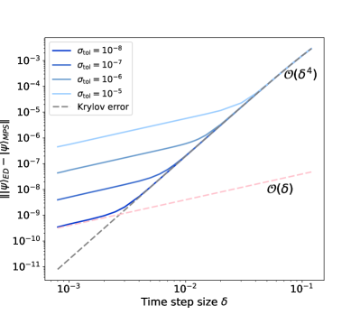
Figure 6: Single step time evolution errors for H2O when using Krylov subspace time evolution based on our THC-MPO for different truncation tolerance $\sigma_{\text{tol}}$, plotted as functions of the time step sizes. The pink dotted line indicates that the truncation error scales linearly for a single time step when utilizing a fixed truncation tolerance, which means a selected truncation tolerance will lead to constant error for a fixed duration regardless of the step sizes.

We also study the Krylov subspace time evolution based on our THC-MPO, where we set the subspace dimension to $4$, leading to a single step error $\mathcal{O}(\delta^{4})$. The initial state is defined as $\ket{\psi(t=0)}=a_{2,\downarrow}\ket{\psi_{0}}$, where a spin-down electron is annihilated from the second spatial orbital of the ground state. Three factors determine the accuracy: SVD cutoff (bond dimension limitation), time step size $\delta$, and the THC error from the THC factorization. The THC error is negligible for the water molecule since the THC rank $N=4L$ results in a very accurate approximation. As depicted in Fig. 6, the behavior of the errors can be well explained: as expected, the Krylov error dominates the overall error for larger time step sizes. Conversely, the $\mathcal{O}(\delta^{4})$ scaling leads to small Krylov errors when the step size $\delta$ is reduced, causing the truncation error to dominate the overall error. When setting the truncation tolerance to $\sigma_{\text{tol}}=10^{-8}$ for which the maximum bond dimension reaches 51, our method can accurately simulate dynamics for step sizes as small as 0.003 a.u. (approximately 0.07 attoseconds) while maintaining the accuracy of the Krylov method. Note that the maximum bond dimension of the time-evolved MPS could grow exponentially over time; therefore, a larger maximum bond dimension is necessary for accurate long-term dynamics. The errors are measured by the distance $\lVert\ket{\psi}_{\text{ED}}-\ket{\psi}_{\text{MPS}}\rVert$ between the states from our numerical method and the reference time-evolved quantum state obtained by ED. This metric is also used to measure the Krylov errors.

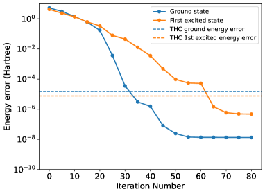
Figure 7: Energy convergence for the hydrogen chain. We restart the iteration at the 60th step to improve the orthogonality of Krylov vectors. The Krylov space is obtained via THC-MPO, while the energy is calculated according to the exact Hamiltonian. The dotted lines describe THC energy errors estimated by diagonalizing the approximated Hamiltonian reconstructed from THC tensors.

A way to reduce computational cost at the expense of accuracy is using a smaller THC rank $N$. To explore this possibility and quantify the resulting error, we study the hydrogen chain of eight atoms with distances of 1.4 Bohr in the STO-6G basis, which leads to 8 spatial orbitals. The THC rank is set to $21$, leading to an overall energy error of $\sim 10^{-5}$, much larger than the previous H2O case. The MPS bond dimensions for representing Krylov vectors are capped at 150. Like the previous example, we again use the Hartree-Fock ground and single-excited states as the initial states for the Krylov method. Interestingly, when using the exact Hamiltonian to calculate the energy expectation value for the approximated ground state:

$$E_{\text{avg,Krylov}}=\bra{\psi_{\text{approx}}}H_{\text{exact}}\ket{\psi_{\text{approx}}},$$ (18)

where $\ket{\psi_{\text{approx}}}$ is obtained by the THC-MPO-based Krylov method and $H_{\text{exact}}$ is the exact Hamiltonian, the resulting energy error is smaller than the error introduced by the THC approximation, as illustrated in Fig. 7. While the THC approximation leads to an energy error of around $10^{-5}$ Hartree, we can obtain the ground and first excited state with energy error $\sim 10^{-8}$ and $\sim 10^{-7}$ Hartree, respectively. This indicates that accurate results could still be obtained using the THC-MPO, even when choosing a smaller THC rank that introduces non-negligible errors.

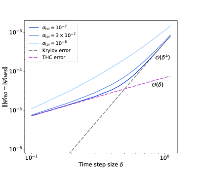
Figure 8: Single step time evolution errors for the hydrogen chain and various truncation tolerances $\sigma_{\text{tol}}$. The initial state is chosen as $\ket{\psi(t=0)}=a_{i}\ket{\psi_{0}}$. The reachable accuracy is bounded by the THC and Krylov errors, especially for small truncation tolerance. The errors are measured by the distance to the numerically exact ED state.

The corresponding time evolution is shown in Fig. 8. Unlike the H2O case, the THC approximation introduces errors comparable to the truncation errors. Consequently, the accuracy is bounded by the maximum of the THC and Krylov errors. One can reach a sweet spot at the intersection of the two dotted lines in Fig. 8. In practice, we recommend using the step size and bond dimension settings where the results have converged, which indicates that the THC approximation limits the accuracy. Additionally, one can increase the THC rank $N$ to enhance accuracy. The error $\lVert v-v^{\prime}\rVert$ can be reduced to $\sim 10^{-8}$ when likewise using $N=4L$ in the present hydrogen chain example.

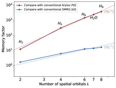
Figure 9: Comparison of memory consumption for the Krylov method based on the conventional MPO versus the THC-MPO (red), as well as DMRG algorithm versus the Krylov method based on the THC-MPO (blue). The maximum bond dimensions are 4, 16, 60, 70, and 80, respectively. The dotted lines representing $\mathcal{O}(L^{4})$ and $\mathcal{O}(L^{2})$ demonstrate that the scaling of $P/Q$ and $S/Q$ aligns well with the theoretical prediction.

One of the advantages of our THC-MPO method is the significantly reduced memory cost by a factor $\mathcal{O}(L^{4})$, as discussed in Sect. III.2. We separately monitored memory consumption to store intermediate MPS in the Krylov algorithm based on the conventional MPO and the THC-MPO to test this prediction in our numerical experiments. We denote memory consumption when using conventional MPOs as $P$, and when using THC-MPOs as $Q$. Fig. 9 shows the quotient $P/Q$ for the water molecule and hydrogen chains. By studying systems of different sizes, one clearly observes the predicted $\mathcal{O}(L^{4})$ scaling. For example, considering the hydrogen chain of eight atoms, the memory required for storing an intermediate state $H\ket{\psi}$ calculated with the conventional MPO amounts to 12586 MB. In contrast, only 3.49 MB is needed when using the THC-MPO method, leading to a factor $P/Q$ as large as 3606. This case’s maximum bond dimension is $80$, and we utilized double-precision complex numbers. The Krylov method based on THC-MPO also outperforms the DMRG algorithm in terms of memory usage. Theoretically, the DMRG algorithm requires $\mathcal{O}(L^{3}M^{2})$ memory (to store the left and right environment blocks), which is $\mathcal{O}(L^{2})$ times larger than the THC-MPO-based Krylov method. As shown in Fig. 9, we numerically compare $Q$ with the memory consumption $S$ for the DMRG algorithm, using the same MPS bond dimensions. The results suggest that our method requires significantly less memory than the DMRG algorithm, and the observed values agree with the theoretically predicted $\mathcal{O}(L^{2})$ scaling. Since the TDVP method could be implemented within a framework similar to the DMRG algorithm, our method also outperforms TDVP in terms of memory consumption.

IV.2 Computational complexity estimation

Besides memory consumption, the global Krylov methods based on our THC-MPO also perform better in terms of computational cost scaling than global Krylov methods using conventional MPOs. Here, we only present the summary; see Appendix B for a detailed derivation.

The primary contributor to the overall cost is obtaining compressed Krylov vectors. When using the conventional MPO construction, renormalization is the most expensive step in this process. Since we have to handle the intermediate MPS with bond dimension $\mathcal{O}(L^{2}M)$, the renormalization has an overall complexity of $\mathcal{O}(L^{7}M^{3})$ for all sites. Meanwhile, for global Krylov methods utilizing THC-MPO, we only need to deal with MPS with bond dimension $\mathcal{O}(M)$ since the bond dimension of each sub-term $G_{\mu\sigma,\nu\sigma^{\prime}}\ket{\psi}$ is twice the bond dimension of $\ket{\psi}$. Therefore, it costs $\mathcal{O}(LM^{3})$ to obtain $G_{\mu\sigma,\nu\sigma^{\prime}}\ket{\psi}$ as compressed MPS, leading to an overall cost of $\mathcal{O}(L^{3}M^{3})$ for all $G_{\mu\sigma,\nu\sigma^{\prime}}\ket{\psi}$ (when assuming that the THC rank $N$ scales linearly with $L$). This computational cost has a large pre-factor; it could be around $10^{5}$ when taking hydrogen chains as an example. The large pre-factor leads to longer run times for small molecules, but we expect an advantage for medium- and large-sized molecules due to its promising scaling gap $\mathcal{O}(L^{4})$. However, the Krylov method using conventional MPOs might be infeasible in practice for medium-sized or large systems due to the large memory requirements.

IV.3 A natural parallelization scheme

Figure 10: Parallelization scheme for applying the Coulomb operator $V$ to a state $\ket{\psi}$ in MPS form according to Eq. (15). Each core is first assigned the sub-task to compute and compress an intermediate state $G_{\mu\sigma,\nu\sigma^{\prime}}\ket{\psi}$ as MPS. These are then aggregated through a reduction process. For simplicity, we assume that the high-performance computer has at least $4N^{2}$ cores; otherwise, a single core would handle several of the $G_{\mu\sigma,\nu\sigma^{\prime}}\ket{\psi}$ states.

Parallel computing has been effectively integrated into DMRG algorithms for quantum chemistry to take advantage of high-performance computing platforms. This integration has significantly enhanced the ability to study large molecular systems; various parallel schemes were proposed [68, 69, 70, 71, 72, 11], and notable open-source packages like Block2 were developed [73]. The Krylov method based on our THC-MPO can straightforwardly use the potential of parallel computing: to obtain $H\ket{\psi}$ following Eq. (15), each of the $4N^{2}$ sub-terms can be calculated and compressed independently, and the summation of these sub-terms can also be performed in parallel by a reduction.

More specifically, we propose a parallelism scheme as illustrated in Fig. 10. For each core, we first assign the task of computing and compressing one (or several) sub-terms $G_{\mu\sigma,\nu\sigma^{\prime}}\ket{\psi}$. The power of multiple cores can be perfectly utilized for this part. After this step, we add and compress these terms pairwise in parallel. It appears that some cores are idling during such a process, but the compression can utilize multiple cores for parallel computation when using packages like multithreaded LAPACK implementations [74]. Because the SVD and QR decomposition can be significantly sped up by parallel computing [75, 76], the reduction part can well utilize the power of parallel computing as well. To employ the optimization which reuses intermediate states $G_{\nu\sigma^{\prime}}\ket{\psi}$ as discussed in Sec. III.2, one can compute all $G_{\nu\sigma^{\prime}}\ket{\psi}$ terms in advance or calculate them dynamically as the computation progresses to the corresponding $\nu\sigma^{\prime}$ index.

In summary, under ideal parallelization conditions with $4N^{2}$ available cores, the parallel runtime scales as $\mathcal{O}(LM^{3})$.

V Conclusions

The THC-MPO approach allows us to implement Krylov subspace methods, e.g., the Lanczos algorithm and Krylov subspace time evolution, with reduced memory usage and lower computational cost. When compared to the Krylov method based on the conventional MPO representation, the memory advantage of THC-MPO is apparent, even for the smallest molecules. Moreover, it outperforms popular methods like DMRG and TDVP in terms of memory consumption, suggesting that THC-MPO can potentially enable simulations of even larger systems than currently reachable by DMRG or TDVP. While the benefit of computational cost is not immediate for small molecules due to large prefactors, we expect that the improvement will become significant for moderate and large molecular systems.

We have not theoretically addressed how the large number of truncations affects the overall error. Although our numerical experiments show that it only leads to slightly larger MPS bond dimensions for obtaining the desired accuracy, the effect should be studied in detail for larger systems. Our THC-MPO method might ameliorate this issue since it enables larger bond dimensions.

The THC-MPO method is compatible with and can be integrated into existing tensor network codes. Abelian quantum number conservation laws (electron number and spin) endow the individual MPS and MPO tensors with a sparsity structure that can help accelerate computations.

A cornerstone of our work is the compressed THC representation of the two-body integral tensor $v$. A promising research direction (complementary to the present study) could be the exploitation of sparsity structures of $v$, for example, due to localized orbitals or wavelet-type orbitals supported on a fine grid.

Using our THC-MPO method and optimized high-performance computing implementations, we plan to explore these ideas and the reachable system sizes in future works.

Appendix A Decomposition of the kinetic term

The matrix $(t_{pq})$ of one-body integrals is real symmetric and can thus be diagonalized via an orthogonal matrix $(u_{pi})$ of eigenvectors and corresponding eigenvalues $\lambda_{i}$:

$$t_{pq}=\sum^{L}_{i=1}u_{pi}\lambda_{i}u_{qi}\quad\text{for all }p,q=1,\dots,L.$$ (19)

Inserted into the kinetic term in Eq. (1), we directly obtain:

$$T=\sum^{L}_{i=1}\sum_{\sigma\in\{\uparrow,\downarrow\}}\underbrace{\lambda_{i}\left(\sum^{L}_{p=1}u_{pi}a^{\dagger}_{p,\sigma}\right)\left(\sum^{L}_{q=1}u_{qi}a_{q,\sigma}\right)}_{=T_{i,\sigma}}.$$ (20)

For each sub-term $T_{i,\sigma}$, one can construct elementary MPOs for $\sum^{L}_{p=1}u_{pi}a^{\dagger}_{p,\sigma}$ and $\sum^{L}_{q=1}u_{qi}a_{q,\sigma}$ in the same way as in Eq. (13). Therefore, $T_{i,\sigma}$ is a product of two MPOs with individual bond dimensions 2. Since the kinetic term is the sum of the sub-terms $T_{i,\sigma}$, the operation $T\ket{\psi}$ can be performed analogously to the Coulomb interaction by sequential summation and compression of the states $T_{i,\sigma}\ket{\psi}$ in MPS form. In total, there are $2L$ sub-terms for the kinetic part, which is relatively small compared to the $\mathcal{O}(L^{2})$ sub-terms arising from the Coulomb interaction. Moreover, note that the spectral decomposition (19) is numerically exact, while the THC representation of the Coulomb overlap integrals in Eq. (2) is an approximation in general.

Appendix B Computational cost estimate for computing Krylov vectors

There are three primary steps to compute $H\ket{\psi}$ in compressed MPS form: multiplying $H$ with $\ket{\psi}$, renormalization, and truncation by SVD. Regarding the conventional MPO-based method, the most expensive step is renormalization, which contains QR decompositions and the subsequent absorption of the $R$ matrices from the QR decomposition into the next site. The QR decomposition on tensors of shape $(2,L^{2}M,L^{2}M)$ leads to a cost of $\sim\frac{10}{3}L^{6}M^{3}$ floating point operations if the Householder reflection method is utilized [77]. Such a decomposition results in an $R$ matrix of shape $(L^{2}M,L^{2}M)$, absorbing it into the next site costs $\sim 2L^{6}M^{3}$. The leading term in computational cost is $\sim\frac{32}{3}L^{7}M^{3}$ floating point operations for all $2L$ sites (spin-orbitals). The SVD cost is minor: starting from the very left or right side, one of the two MPS virtual bonds has already been reduced to $M$, leading to a tensor of shape $(2,M,L^{2}M)$. Applying an SVD of such a tensor only costs $\mathcal{O}(L^{2}M^{3})$, which is much smaller than the cost from the QR decomposition. The asymptotic scaling $\mathcal{O}(L^{7}M^{3})$ is a significant hurdle when applying global methods to large systems. Typically, the maximum MPO bond dimensions exceed $L^{2}$, so we provide only a rough estimation to offer some intuition.

For THC-MPO, we first discuss the computational complexity of evaluating a sub-term $G_{\mu\sigma,\nu\sigma^{\prime}}\ket{\psi}$, for which we execute multiplication and compression layer by layer as discussed in III.2. After multiplying a layer with the current MPS, the shape of the resulting temporary MPS tensors is $(2,2M,2M)$ since the MPO bond dimension for each layer is 2. Thus, employing a single-site QR decomposition costs $\sim\frac{80}{3}M^{3}$ floating point operations. Subsequently, absorbing the $R$ matrix of shape $(2M,2M)$ into the next site costs $\sim 16M^{3}$. Finally, we apply an SVD to truncate the intermediate MPS. Similarly to the conventional case, one of the two MPS virtual bonds has already been reduced to $M$, leading to a tensor of shape $(2,M,2M)$. Applying an SVD of such a tensor costs $\sim 56M^{3}$ [77] using the divide-and-conquer method implemented in LAPACK [78, 79], and absorbing the obtained matrix into the next site costs $\sim 8M^{3}$. In summary, for each of the four layers in $G_{\mu\sigma,\nu\sigma^{\prime}}$ it costs $\sim 214LM^{3}$ to compress the intermediate MPS for all $2L$ sites, leading to $\sim 10^{3}LM^{3}$ floating point operations to obtain $G_{\mu\sigma,\nu\sigma^{\prime}}\ket{\psi}$ in compressed MPS form. To implement Eq. (15), one needs to execute $4N^{2}$ times multiplication-compression and $4N^{2}-1$ times addition-compression, where $N$ is the THC rank which scales linearly with system size. Taking the hydrogen chain with $N=3L-3$ as an example, this leads to a total cost of $\sim 10^{5}L^{3}M^{3}$ floating point operations, considering the optimization in which we re-use the later half of $G_{\mu\sigma,\nu\sigma^{\prime}}$, as mentioned in Sec. III.2.

Even though the complexity estimation here is approximate since we do not consider sparsity and treat all bond dimensions as $M$ for simplicity, the asymptotic scaling gap $\mathcal{O}(L^{4})$ is faithfully captured. Comparing the cost $\sim 10L^{7}M^{3}$ for a conventional MPO with $\sim 10^{5}L^{3}M^{3}$ for the THC-MPO method, the crossover point is estimated to occur when $L$ is in the range of a few tens.

References

- Östlund and Rommer [1995] S. Östlund and S. Rommer, Thermodynamic limit of density matrix renormalization, Phys. Rev. Lett. 75, 3537 (1995).
- Rommer and Östlund [1997] S. Rommer and S. Östlund, Class of ansatz wave functions for one-dimensional spin systems and their relation to the density matrix renormalization group, Phys. Rev. B 55, 2164 (1997).
- Ma et al. [2022] H. Ma, U. Schollwöck, and Z. Shuai, Density Matrix Renormalization Group (DMRG)-Based Approaches in Computational Chemistry (Elsevier, 2022).
- Chan and Sharma [2011] G. K.-L. Chan and S. Sharma, The density matrix renormalization group in quantum chemistry, Annu. Rev. Phys. Chem. 62, 465 (2011).
- Xu et al. [2022] Y. Xu, Z. Xie, X. Xie, U. Schollwöck, and H. Ma, Stochastic adaptive single-site time-dependent variational principle, JACS Au 2, 335 (2022).
- Ren et al. [2018] J. Ren, Z. Shuai, and G. Kin-Lic Chan, Time-dependent density matrix renormalization group algorithms for nearly exact absorption and fluorescence spectra of molecular aggregates at both zero and finite temperature, J. Chem. Theory Comput. 14, 5027 (2018).
- Baiardi et al. [2017] A. Baiardi, C. J. Stein, V. Barone, and M. Reiher, Vibrational density matrix renormalization group, J. Chem. Theory Comput. 13, 3764 (2017).
- White [1992] S. R. White, Density matrix formulation for quantum renormalization groups, Phys. Rev. Lett. 69, 2863 (1992).
- White [1993] S. R. White, Density-matrix algorithms for quantum renormalization groups, Phys. Rev. B 48, 10345 (1993).
- Xu et al. [2023] Y. Xu, Y. Cheng, Y. Song, and H. Ma, New density matrix renormalization group approaches for strongly correlated systems coupled with large environments, J. Chem. Theory Comput. 19, 4781 (2023).
- Chan et al. [2016] G. K. Chan, A. Keselman, N. Nakatani, Z. Li, and S. R. White, Matrix product operators, matrix product states, and ab initio density matrix renormalization group algorithms, J. Chem. Phys. 145 (2016).
- Keller et al. [2015] S. Keller, M. Dolfi, M. Troyer, and M. Reiher, An efficient matrix product operator representation of the quantum chemical Hamiltonian, J. Chem. Phys. 143, 244118 (2015).
- Szalay et al. [2015] S. Szalay, M. Pfeffer, V. Murg, G. Barcza, F. Verstraete, R. Schneider, and O. Legeza, Tensor product methods and entanglement optimization for ab initio quantum chemistry, Int. J. Quantum Chem. 115, 1342 (2015).
- Friesecke et al. [2024] G. Friesecke, G. Barcza, and Ö. Legeza, Predicting the FCI energy of large systems to chemical accuracy from restricted active space density matrix renormalization group calculations., J. Chem. Theory Comput. 20, 87 (2024).
- Cheng and Ma [2024] Y. Cheng and H. Ma, Renormalized-residue-based multireference configuration interaction method for strongly correlated systems, J. Chem. Theory and Comput. 20, 1988 (2024).
- Klünder et al. [2011] K. Klünder, J. M. Dahlström, M. Gisselbrecht, T. Fordell, M. Swoboda, D. Guénot, P. Johnsson, J. Caillat, J. Mauritsson, A. Maquet, R. Taïeb, and A. L’Huillier, Probing single-photon ionization on the attosecond time scale, Phys. Rev. Lett. 106, 143002 (2011).
- Krausz and Ivanov [2009] F. Krausz and M. Ivanov, Attosecond physics, Rev. Mod. Phys. 81, 163 (2009).
- Lépine et al. [2014] F. Lépine, M. Y. Ivanov, and M. J. Vrakking, Attosecond molecular dynamics: fact or fiction?, Nat. Photonics 8, 195 (2014).
- Goulielmakis et al. [2010] E. Goulielmakis, Z.-H. Loh, A. Wirth, R. Santra, N. Rohringer, V. S. Yakovlev, S. Zherebtsov, T. Pfeifer, A. M. Azzeer, M. F. Kling, S. R. Leone, and F. Krausz, Real-time observation of valence electron motion, Nature 466, 739 (2010).
- Nisoli et al. [2017] M. Nisoli, P. Decleva, F. Calegari, A. Palacios, and F. Martín, Attosecond electron dynamics in molecules, Chem. Rev. 117, 10760 (2017).
- Baltuška et al. [2003] A. Baltuška, T. Udem, M. Uiberacker, M. Hentschel, E. Goulielmakis, C. Gohle, R. Holzwarth, V. S. Yakovlev, A. Scrinzi, T. W. Hänsch, and F. Krausz, Attosecond control of electronic processes by intense light fields, Nature 421, 611 (2003).
- Borrego-Varillas et al. [2022] R. Borrego-Varillas, M. Lucchini, and M. Nisoli, Attosecond spectroscopy for the investigation of ultrafast dynamics in atomic, molecular and solid-state physics, Rep. Prog. Phys. 85, 066401 (2022).
- Midorikawa [2022] K. Midorikawa, Progress on table-top isolated attosecond light sources, Nat. Photon. 16, 267 (2022).
- Haegeman et al. [2016] J. Haegeman, C. Lubich, I. Oseledets, B. Vandereycken, and F. Verstraete, Unifying time evolution and optimization with matrix product states, Phys. Rev. B 94, 165116 (2016).
- Baiardi and Reiher [2019] A. Baiardi and M. Reiher, The density matrix renormalization group in chemistry and molecular physics: Recent developments and new challenges., J. Chem. Phys. 152 4, 040903 (2019).
- Baiardi [2021] A. Baiardi, Electron dynamics with the time-dependent density matrix renormalization group, J. Chem. Theory Comput. 17, 3320 (2021).
- Ren et al. [2022] J. Ren, W. Li, T. Jiang, Y. Wang, and Z. Shuai, Time-dependent density matrix renormalization group method for quantum dynamics in complex systems, WIREs Comput. Mol. Sci. 12, e1614 (2022).
- Xu et al. [2024] Y. Xu, C. Liu, and H. Ma, Kylin-V: An open-source package calculating the dynamic and spectroscopic properties of large systems, J. Chem. Phys. 161 (2024).
- Hu and Chan [2015] W. Hu and G. K.-L. Chan, Excited-state geometry optimization with the density matrix renormalization group, as applied to polyenes., J. Chem. Theory Comput. 11 7, 3000 (2015).
- Kloss et al. [2018] B. Kloss, Y. B. Lev, and D. Reichman, Time-dependent variational principle in matrix-product state manifolds: Pitfalls and potential, Phys. Rev. B 97, 024307 (2018).
- Goto and Danshita [2019] S. Goto and I. Danshita, Performance of the time-dependent variational principle for matrix product states in the long-time evolution of a pure state, Phys. Rev. B 99, 054307 (2019).
- Yang and White [2020] M. Yang and S. R. White, Time-dependent variational principle with ancillary Krylov subspace, Phys. Rev. B 102, 094315 (2020).
- Paeckel et al. [2019] S. Paeckel, T. Köhler, A. Swoboda, S. R. Manmana, U. Schollwöck, and C. Hubig, Time-evolution methods for matrix-product states, Annals of Physics 411, 167998 (2019).
- Haydock [1980] R. Haydock, The recursive solution of the Schrödinger equation, Solid State Phys. 35, 215 (1980).
- Lanczos [1950] C. Lanczos, An iteration method for the solution of the eigenvalue problem of linear differential and integral operators, J. Res. Nat. Bur. Stand. 45, 255 (1950).
- Dargel et al. [2012] P. E. Dargel, A. Woellert, A. Honecker, I. McCulloch, U. Schollwöck, and T. Pruschke, Lanczos algorithm with matrix product states for dynamical correlation functions, Phys. Rev. B 85, 205119 (2012).
- Note [1] There is also a “local version” for the Krylov method used in DMRG and time evolution simulation [33]; in this paper, we solely focus on the global Krylov method introduced in Sec. II.2.
- Ronca et al. [2017] E. Ronca, Z. Li, C. A. Jimenez-Hoyos, and G. K.-L. Chan, Time-step targeting time-dependent and dynamical density matrix renormalization group algorithms with ab initio Hamiltonians, J. Chem. Theory Comput. 13, 5560 (2017).
- Frahm and Pfannkuche [2019] L.-H. Frahm and D. Pfannkuche, Ultrafast ab initio quantum chemistry using matrix product states, J. Chem. Theory Comput. 15, 2154 (2019).
- Ren et al. [2020] J. Ren, W. Li, T. Jiang, and Z. Shuai, A general automatic method for optimal construction of matrix product operators using bipartite graph theory, J. Chem. Phys. 153 (2020).
- Schollwöck [2011] U. Schollwöck, The density-matrix renormalization group in the age of matrix product states, Annals of Physics 326, 96 (2011).
- Ma et al. [2024] L. Ma, M. Fishman, M. Stoudenmire, and E. Solomonik, Approximate contraction of arbitrary tensor networks with a flexible and efficient density matrix algorithm, arXiv:2406.09769 (2024), 2406.09769 .
- Hohenstein et al. [2012a] E. G. Hohenstein, R. M. Parrish, and T. J. Martínez, Tensor hypercontraction density fitting. I. Quartic scaling second-and third-order Møller-Plesset perturbation theory, J. Chem. Phys. 137 (2012a).
- Parrish et al. [2012] R. M. Parrish, E. G. Hohenstein, T. J. Martínez, and C. D. Sherrill, Tensor hypercontraction. II. Least-squares renormalization, J. Chem. Phys. 137 (2012).
- Hohenstein et al. [2012b] E. G. Hohenstein, R. M. Parrish, C. D. Sherrill, and T. J. Martínez, Communication: Tensor hypercontraction. III. Least-squares tensor hypercontraction for the determination of correlated wavefunctions, J. Chem. Phys. 137 (2012b).
- Bridgeman and Chubb [2017] J. C. Bridgeman and C. T. Chubb, Hand-waving and interpretive dance: An introductory course on tensor networks, J. Phys. A: Math. Theor. 50, 223001 (2017).
- Dargel et al. [2011] P. E. Dargel, A. Honecker, R. Peters, R. M. Noack, and T. Pruschke, Adaptive Lanczos-vector method for dynamic properties within the density matrix renormalization group, Phys. Rev. B 83, 161104 (2011).
- Park and Light [1986] T. J. Park and J. Light, Unitary quantum time evolution by iterative Lanczos reduction, J. Chem. Phys. 85, 5870 (1986).
- Kosloff [1988] R. Kosloff, Time-dependent quantum-mechanical methods for molecular dynamics, J. Phys. Chem. 92, 2087 (1988).
- Hochbruck and Lubich [1997] M. Hochbruck and C. Lubich, On Krylov subspace approximations to the matrix exponential operator, SIAM J. Numer. Anal. 34, 1911 (1997).
- Saad [1980] Y. Saad, Variations on Arnoldi’s method for computing eigenelements of large unsymmetric matrices, Lin. Alg. Appl. 34, 269 (1980).
- Hauschild and Pollmann [2018] J. Hauschild and F. Pollmann, Efficient numerical simulations with tensor networks: Tensor Network Python (TeNPy), SciPost Phys. Lect. Notes , 5 (2018).
- Stoudenmire and White [2010] E. M. Stoudenmire and S. R. White, Minimally entangled typical thermal state algorithms, New J. Phys. 12, 055026 (2010).
- Lee et al. [2019] J. Lee, L. Lin, and M. Head-Gordon, Systematically improvable tensor hypercontraction: Interpolative separable density-fitting for molecules applied to exact exchange, second-and third-order Møller–Plesset perturbation theory, J. Chem. Theory Comput. 16, 243 (2019).
- Parrish et al. [2014] R. M. Parrish, C. D. Sherrill, E. G. Hohenstein, S. I. Kokkila, and T. J. Martínez, Communication: Acceleration of coupled cluster singles and doubles via orbital-weighted least-squares tensor hypercontraction, J. Chem. Phys. 140 (2014).
- Schutski et al. [2017] R. Schutski, J. Zhao, T. M. Henderson, and G. E. Scuseria, Tensor-structured coupled cluster theory, J. Chem. Phys. 147 (2017).
- Lu and Ying [2015] J. Lu and L. Ying, Compression of the electron repulsion integral tensor in tensor hypercontraction format with cubic scaling cost, J. Comput. Phys. 302, 329 (2015).
- Whitten [1973] J. L. Whitten, Coulombic potential energy integrals and approximations, J. Chem. Phys. 58, 4496 (1973).
- Dunlap et al. [1979] B. I. Dunlap, J. Connolly, and J. Sabin, On some approximations in applications of x theory, J. Chem. Phys. 71, 3396 (1979).
- Werner et al. [2003] H.-J. Werner, F. R. Manby, and P. J. Knowles, Fast linear scaling second-order Møller–Plesset perturbation theory (MP2) using local and density fitting approximations, J. Chem. Phys. 118, 8149 (2003).
- Hu et al. [2017] W. Hu, L. Lin, and C. Yang, Interpolative separable density fitting decomposition for accelerating hybrid density functional calculations with applications to defects in silicon, J. Chem. Theory Comput. 13, 5420 (2017).
- Duchi et al. [2011] J. Duchi, E. Hazan, and Y. Singer, Adaptive subgradient methods for online learning and stochastic optimization., J. Mach. Learn. Res. 12 (2011).
- opt [2024] https://github.com/google-deepmind/optax (2024).
- Jordan and Wigner [1928] P. Jordan and E. Wigner, Über das Paulische Äquivalenzverbot, Zeitschrift für Physik 47, 631 (1928).
- Sun et al. [2018] Q. Sun, T. C. Berkelbach, N. S. Blunt, G. H. Booth, S. Guo, Z. Li, J. Liu, J. D. McClain, E. R. Sayfutyarova, S. Sharma, S. Wouters, and G. K.-L. Chan, PySCF: the Python-based simulations of chemistry framework, WIREs Comput. Mol. Sci. 8, e1340 (2018).
- Sun et al. [2020] Q. Sun, X. Zhang, S. Banerjee, P. Bao, M. Barbry, N. S. Blunt, N. A. Bogdanov, G. H. Booth, J. Chen, Z.-H. Cui, et al., Recent developments in the PySCF program package, J. Chem. Phys. 153, 024109 (2020).
- Mendl [2018] C. B. Mendl, PyTeNet: A concise Python implementation of quantum tensor network algorithms, J. Open Source Softw. 3, 948 (2018).
- Zhai and Chan [2021] H. Zhai and G. K. Chan, Low communication high performance ab initio density matrix renormalization group algorithms, J. Chem. Phys. 154, 224116 (2021).
- Xiang et al. [2024] C. Xiang, W. Jia, W.-H. Fang, and Z. Li, Distributed multi-GPU ab initio density matrix renormalization group algorithm with applications to the P-cluster of nitrogenase, J. Chem. Theory Comput. 20, 775 (2024).
- Olivares-Amaya et al. [2015] R. Olivares-Amaya, W. Hu, N. Nakatani, S. Sharma, J. Yang, and G. K.-L. Chan, The ab-initio density matrix renormalization group in practice, J. Chem. Phys. 142, 034102 (2015).
- Chan [2004] G. K.-L. Chan, An algorithm for large scale density matrix renormalization group calculations, J. Chem. Phys. 120, 3172 (2004).
- Wouters and Van Neck [2014] S. Wouters and D. Van Neck, The density matrix renormalization group for ab initio quantum chemistry, Eur. Phys. J. D 68, 1 (2014).
- Zhai et al. [2023] H. Zhai, H. R. Larsson, S. Lee, Z.-H. Cui, T. Zhu, C. Sun, L. Peng, R. Peng, K. Liao, J. Tlle, J. Yang, S. Li, and G. K.-L. Chan, Block2: A comprehensive open source framework to develop and apply state-of-the-art DMRG algorithms in electronic structure and beyond, J. Chem. Phys. 159, 234801 (2023).
- Blackford et al. [2002] L. S. Blackford, J. Demmel, J. Dongarra, I. Duff, S. Hammarling, G. Henry, M. Heroux, L. Kaufman, A. Lumsdaine, A. Petitet, R. Pozo, K. Remington, and R. C. Whaley, An updated set of basic linear algebra subprograms (BLAS), ACM Trans. Math. Softw. 28, 135 (2002).
- Demmel et al. [2012] J. Demmel, L. Grigori, M. Hoemmen, and J. Langou, Communication-optimal parallel and sequential QR and LU factorizations, SIAM J. Sci. Comput. 34, A206 (2012).
- Jessup and Sorensen [1994] E. R. Jessup and D. C. Sorensen, A parallel algorithm for computing the singular value decomposition of a matrix, SIAM J. Matrix Anal. Appl. 15, 530 (1994).
- Golub and Van Loan [2013] G. H. Golub and C. F. Van Loan, Matrix Computations (Johns Hopkins University Press, 2013).
- Gu and Eisenstat [1996] M. Gu and S. C. Eisenstat, Efficient algorithms for computing a strong rank-revealing QR factorization, SIAM J. Sci. Comput. 17, 848 (1996).
- Anderson et al. [1999] E. Anderson, Z. Bai, C. Bischof, L. S. Blackford, J. Demmel, J. Dongarra, J. Du Croz, A. Greenbaum, S. Hammarling, A. McKenney, and D. Sorensen, LAPACK Users’ Guide (Society for Industrial and Applied Mathematics, 1999).