Resource Allocation in Distributed Quantum Computing Interconnect Networks

Abstract

Distributed quantum computing (DQC) has emerged as a promising approach to overcome the scalability limitations of monolithic quantum processors in terms of computing capability. However, realising the full potential of DQC requires effective resource allocation. This involves efficiently distributing quantum circuits across the network by assigning each circuit to an optimal subset of quantum processing units (QPUs), based on factors such as their computational power and connectivity. In heterogeneous DQC networks with arbitrary topologies and non-identical QPUs, resource allocation becomes a complex challenge. This paper addresses the problem of resource allocation in such networks, focusing on computing resource management in a quantum farm setting. We propose a multi-objective optimisation algorithm for optimal QPU allocation that aims to minimise the degradation caused by inter-QPU communication latencies due to qubit decoherence, while maximising the number of concurrently assignable quantum circuits. The algorithm takes into account several key factors, including the network topology, QPU characteristics, and quantum circuit structure, to make efficient allocation decisions. We formulate the optimisation problem as a mixed-integer linear program and solve it using standard optimisation tools. Simulation results demonstrate the effectiveness of the proposed algorithm in minimising communication costs and improving resource utilisation compared to a benchmark greedy allocation approach. To complement our proposed QPU allocation method, we also present a compatible quantum circuit scheduling model. Our work provides valuable insights into resource allocation strategies for DQC systems and contributes to the development of efficient execution management frameworks for quantum computing.

I Introduction

Quantum computing has emerged as a promising solution for tackling intractable problems, due to its capacity to solve them significantly faster than traditional computers. In recent years, there have been notable advancements in quantum hardware and control systems, leading to the development of noisy intermediate-scale quantum processing units (QPUs). However, despite these efforts, current quantum processors still remain limited in their computational power. In this context, distributed quantum computing (DQC) has emerged as a promising approach to address the scalability limitations of monolithic quantum processors in terms of the number of qubits. [1, 2, 3, 4].

Distributed quantum computing aims to harness the collective power of multiple interconnected quantum processors, enabling the execution of larger and more complex quantum algorithms. In DQC, quantum algorithms are partitioned and executed across a network of quantum processors, which are interconnected through both quantum and classical communication channels. By distributing the computational workload among multiple quantum nodes, this approach facilitates the development of scalable quantum computing systems that can surpass the limitations imposed by individual quantum processors.

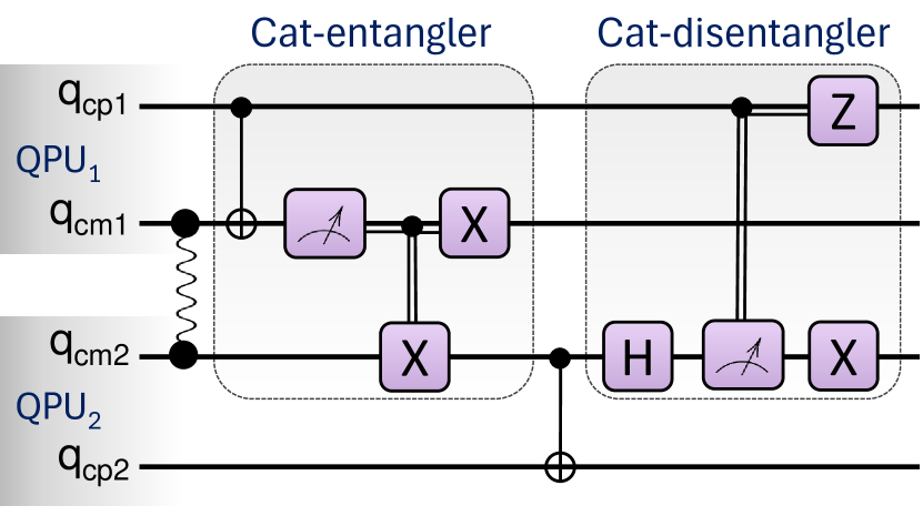
Figure 1: Circuit diagram of remote CNOT gate performed between two QPUs.

Distributed quantum computing is expected to progress through stages of increasing scale and heterogeneity [3]. This progression spans from the integration of multiple quantum processors within a single large quantum computer to the establishment of interconnected quantum processors across various quantum farms. This work focuses on DQC within a single farm, where multiple quantum computers are interconnected via short-to-medium range links. A quantum farm, in this context, refers to a facility housing quantum computers and the infrastructure for their operation and maintenance. A key challenge lies in the introduction of delays caused by inter-node quantum and classical communication. These delays can adversely impact computation accuracy due to the decoherence of qubits over time. Another noteworthy challenge is the efficient execution management for the quantum computing tasks requested by concurrent users.

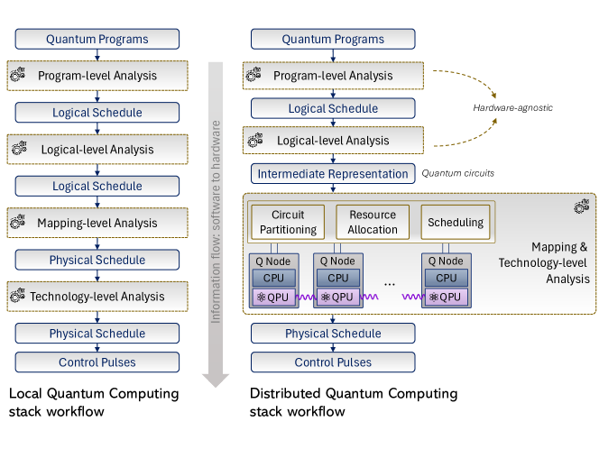
(a)

Figure 2: Workflow of the quantum stack for both local and distributed quantum computing. A layered-oriented approach for compilation tools that bridge quantum algorithms with quantum devices. The stack workflow for local quantum computing, depicted on the left side of the figure, is based on [5].

One of the key requirements for the distributed execution of quantum algorithms is the ability to perform quantum operations between distant qubits residing on separate QPUs. A notable approach to accomplish such remote quantum operations, termed remote gates, utilises two primitives: cat-entangler and cat-disentangler, as proposed by Yimsiriwattana and Lomonaco [1]. This approach involves the utilisation of an entangled pair, local quantum operations on individual QPUs, and classical communication. The cat-entangler creates an entangled state, called a “cat-like state”, between two or more qubits, while the cat-disentangler performs the reverse operation. Figure 1 illustrates the circuit diagram for implementing a controlled-NOT (CNOT) gate based on this approach between two computing qubits, denoted by $q_{\rm cp1}$ and $q_{\rm cp2}$, belonging to separate QPUs (${\rm QPU}_{1}$ and ${\rm QPU}_{2}$). The initial step in this method involves generating entanglement between two dedicated communication qubits, denoted by $q_{\rm cm1}$ and $q_{\rm cm2}$ in Fig. 1, which facilitate the quantum communication between the QPUs. As depicted in the figure, the X operation on ${\rm QPU}_{2}$ and the Z operation on ${\rm QPU}_{1}$ are conditioned on the measurement outcome transmitted classically from the other QPU. This demonstrates that the overall process of remote gate execution involves both quantum and classical communication between QPUs.

The integration of quantum networking, classical networking, and quantum computation within a DQC interconnect network requires efficient orchestration of various components and tasks. A critical element in this orchestration is quantum compilation, which translates a high-level description of a quantum program into a set of instructions to be applied to the physical hardware [6, 5]. This translation is performed through several layers of subroutines forming a compilation stack, as depicted in Fig. 2 [5]. In the context of DQC, several additional tasks must be executed for an intermediate representation of the quantum program, termed Quantum Circuit (QCirc) (Fig. 2). These tasks include scheduling, resource allocation, and circuit partitioning. Scheduling efficiently manages the queue of QCircs in a quantum farm environment, minimising wait times and optimising resource utilisation. Resource allocation assigns computing and communication resources to QCircs, including QPUs and, at a finer granularity, specific computing qubits within these QPUs, as well as both classical and quantum communication elements. Circuit partitioning optimises the division of QCircs into smaller sub-circuits, considering the number of partitions, allocated QPUs, and the QCirc’s structure.

This work focuses on QPU allocation and QCirc scheduling, crucial aspects of execution management in a quantum farm. Quantum computing’s unique characteristics, particularly limited qubit coherence time, necessitate resource allocation algorithms that consider not only resource utilisation but also the impact of communication latencies on computation accuracy. Unlike classical computing, where communication latencies primarily affect task completion time, in quantum computing, they can significantly impact computation accuracy. To mitigate qubit decoherence caused by communication delays, effective QPU allocation algorithms must consider the network topology and characteristics, along with the QPUs’ features and limitations, including their capacity (number of computing qubits) and decoherence properties. Additionally, previous research [7] has shown that quantum circuits exhibit different levels of sensitivity to the errors arising from their distributed execution. Therefore, a QPU allocation method that takes the distinctive features of QCircs into account would enhance the overall performance and promote fairness in terms of computation accuracy. Moreover, as QCirc scheduling and QPU allocation are closely interrelated, an efficient scheduling method tailored to the developed QPU allocation strategy is a prerequisite for optimal performance. These factors serve as the primary motivation for this work.

In the following subsections, related work is first outlined, followed by a detailed description of our contributions.

I-A Related work

In the literature, extensive research has focused on quantum compilation and/or circuit partitioning for individual quantum circuits, while relatively limited research efforts have addressed execution management, including QPU allocation. Given the strong interdependencies among these tasks, we present key related works on these topics in what follows.

Several works have explored quantum compilation for DQC. Ferrari et al. [8] discussed challenges in compiler design for DQC and analytically characterised the overhead introduced by remote gates. Cuomo et al. [9] proposed compilation techniques to optimise circuit execution time and distributed entangled state usage. They modeled time as additional circuit depth layers due to entanglement generation, but their approach assumed uniform entanglement latency and neglected network topology. In a subsequent work, Ferrari et al. [10] presented a modular compilation framework incorporating network and QPU constraints. While this framework effectively considers network configuration and QPU characteristics, it primarily focuses on compilation and partitioning for a single circuit assigned to a fixed number of QPUs.

The problem of quantum circuit partitioning has been addressed in multiple research works. Daei et al. [11] represent QCircs as undirected graphs where qubits are nodes and edge weights correspond to the number of two-qubit gates shared between them. They then employ the Kernighan-Lin (K-L) algorithm to partition the graph, minimising the number of edges cut across partitions. In other studies [12, 13, 14, 15], methods such as hypergraph partitioning, bipartite graph partitioning, and genetic algorithms have been employed to minimise the number of remote gates. Andres et al. [16] extended previous works on circuit partitioning to the case of heterogeneous networks with arbitrary topologies. While these studies have focused on optimally partitioning a single QCirc assuming a fixed number of partitions, they have not explicitly considered the issue of resource competition when multiple QCircs are to be concurrently assigned.

Parekh et al. [17] proposed a resource allocation and scheduling algorithm based on a greedy approach that assigns QCircs and fills QPUs on a one-by-one basis. However, their algorithm does not take into account factors such as network topology and configuration, QPU decoherence properties, and the distinctive features of QCircs.

I-B Our contributions

Despite the growing body of literature on compilation and circuit partitioning techniques for individual quantum circuits, there is a notable lack of research addressing execution management in DQC interconnect networks, particularly in the context of quantum farms. In a quantum farm, multiple requests for executing quantum algorithms are submitted simultaneously, raising important questions about optimal resource allocation and scheduling. For instance, determining the appropriate number of partitions for each quantum circuit and the specific QPUs that should be allocated to each circuit becomes a critical challenge. This work aims to address these gaps through the following contributions.

We address the problem of resource allocation, particularly the allocation of QPUs as computing resources, in DQC interconnect networks. We consider a general heterogeneous network model that includes QPUs with varying capacities and decoherence properties, arbitrary network topologies, and diverse types of QCircs. Two primary objectives are considered for the QPU allocation problem: minimising the errors arising from quantum and classical communication latencies, and maximising the number of successfully assigned QCircs. We formulate a multi-objective optimisation problem with these two objectives. The formulated problem takes into account: a) network topology and characteristics, b) QPU capacity (the number of computing qubits) and decoherence properties, and c) quantum circuit structure. We then propose a QPU allocation algorithm based on mixed-integer linear programming (MILP). It is important to note that the first objective is highly correlated and aligns well with the goal of reducing the required communication resources, particularly communication qubits. Consequently, optimising for this objective simultaneously enhances the utilisation of communication resources in the quantum network.

While the main focus of this work is QPU allocation, we recognise that QPU allocation and the scheduling of QCircs are closely related. To address this, we present a scheduling model that complements the proposed QPU allocation algorithm and takes into account the unique features of quantum computing.

II Network Model

We consider a DQC network in which quantum computers, as quantum nodes, are interconnected by quantum and classical links, as illustrated in Fig. 3. We assume that the network may have two types of quantum links: direct and multi-hop. In the case of direct links, two nodes share an entangled pair without the use of any intermediate hop, while in the case of multi-hop links, entanglement swapping is utilised to generate end-to-end entanglement between two nodes not interconnected by a direct quantum link [18]. Regarding the quantum nodes, they may have different capabilities; for instance, some nodes may have entanglement swapping capability, allowing them to function as quantum repeaters (intermediate hops). Furthermore, the QPUs within the nodes may have varying capacities and decoherence properties. These assumptions enable us to consider a highly general quantum network model, where neither the nodes nor the quantum links are required to be identical. Moreover, the logical network topology can be fully-connected or partially-connected. In the following, we provide a more detailed discussion on the quantum and classical links and their associated latencies.

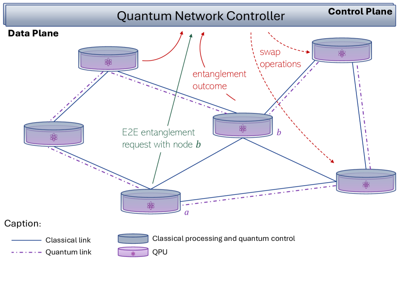
Figure 3: High level representation of a quantum network with basic quantum network operations. A QPU can act as a repeater when capabilities allow.

II-A Quantum communication latency

In the field of quantum communication, it is well-known that entanglement generation is a probabilistic procedure, often requiring multiple attempts for successful creation [19]. The probability of successful entanglement generation depends on various factors, such as link loss, detector efficiency, and the average attempt rate. Furthermore, if entanglement distillation and/or channel multiplexing techniques are employed, the success probability is also influenced by the specific protocol and technique used. In all scenarios, a parameter quantifying the delay introduced by the entanglement generation process can be defined, typically as the inverse of the average entanglement rate. For a given network topology, we assume that each link has a constant delay parameter, which we denote as $T^{\rm eg}_{j_{1}j_{2}}$ for the QPU pair ${\rm{QPU}}_{j_{1}}$ and ${\rm{QPU}}_{j_{2}}$.

II-B Classical communication latency

As depicted in Fig. 1, inter-QPU classical communication is an essential component of remote gate execution. We denote the classical communication latency between the QPU pair ${\rm{QPU}}{j_{1}}$ and ${\rm{QPU}}{j_{2}}$ as $T^{\rm cl}_{j_{1}j_{2}}$. If direct communication between QPUs can be completed in hardware without transferring to the software domain, lower $T^{\rm cl}_{j_{1}j_{2}}$ values and more deterministic behaviour can be achieved. Programmable hardware such as FPGAs plays a key role in the direct interconnection between nodes. These interconnections can be deterministically established within nanoseconds when FPGAs connect the QPUs via optical links for 10GbE, as reported in [7].

III Scheduling Model

The proposed workflow for the QCircs scheduling is presented in Figure 4. The QCircs queued in the QCircs Queue are assigned a priority using a predefined mechanism that may consider parameters such as dependency to other quantum programs, deadline, and wait time. Although the specifics of the priority assignment are beyond the scope of this paper, the wait time of a QCirc significantly influences its priority, preventing starvation from prolonged queuing. We assume that priority assignment occurs regularly, with the QCircs in the queue sorted accordingly, and that each QCirc has a priority $p$.

In our scheduling model, we assume non-preemption, which means that once a QCirc starts execution on the allocated QPUs, it runs to completion without interruption. The network controller selects batches of $M_{i}$ higher-priority QCircs from the QCircs Queue sequentially, where $i$ represents the index of the scheduling cycle. The parameter $M_{i}$ can be dynamically adjusted for each scheduling cycle $i$. We denote the batch of QCircs in the scheduling cycle $i$ by ${{\rm{QCirc}}_{1},{\rm{QCirc}}_{2},\dots,{\rm{QCirc}}_{M_{i}}}$, with priorities ${p_{1},p_{2},\dots,p_{M_{i}}}$, where $p_{1}\geq p_{2}\geq\cdots\geq p_{M_{i}}$. The QCircs in this batch undergo a QPU allocation process, which maps QCircs to the available QPUs. The parameter $M_{i}$ is chosen such that, with a high probability, all QCircs in the batch can be successfully assigned to QPUs. However, to account for the low-probability cases where a small subset of QCircs remains unassigned, a secondary queue called the Overflow Queue is introduced, as shown in Fig. 4. The Overflow Queue handles the remaining unassigned QCircs based on their priority, allocating a QCirc as soon as a subset of QPUs satisfying its specific requirements becomes available. After all the QCircs in the current batch are assigned, the next batch selection cycle begins.

Figure 4: QCirc scheduling in a quantum farm. Batch selection is applied to select a non-fixed amount of QCircs. Within each batch, any QCircs not served (Qcirc_) remain in the Overflow Queue to be later assigned a subset of QPUs based on their priorities.

The proposed scheduling approach leverages the advantages of batch scheduling by considering the specific characteristics of the QCircs and the network. Concurrently, it prevents long waiting times by relaxing the need to wait for the availability of resources for all the QCircs in the Overflow Queue.

IV QPU allocation

As described in the previous section, QPU allocation involves mapping a batch of QCircs to available QPUs. This crucial step significantly impacts resource utilisation, queue waiting time, and overall quantum computing performance, including execution time and accuracy. Here, we propose an optimisation algorithm to optimise the assignment of QCircs to the available QPUs in a specific scheduling cycle. The algorithm aims to optimise two primary objectivesrst objective is minimising the error cost imposed by inter-QPU communication. To accomplish this, we define a cost function that characterises the negative impact of communication latencies between QPUs on quantum computation tasks. Minimising this cost is paramount due to the inherent decoherence experienced by qubits embedded in QPUs over time. The second objective is to maximize the number of concurrently assigned QCircs, thereby reducing both the frequency of overflow queue triggers and its size.

The output of the QPU allocation process consists of three key components: (a) the assigned partition number for each QCirc, (b) the specific QPUs allocated to each QCirc, and (c) the number of qubits per partition. This information is subsequently utilised by the circuit partitioning block to efficiently divide the QCircs into smaller sub-circuits and map the qubits to each sub-circuit appropriately.

IV-A Problem formulation

The set of QPUs in the network is denoted by $\{{\rm{QPU}}_{1},{\rm{QPU}}_{2},\dots,{\rm{QPU}}_{D}\}$, where $D$ represents the total number of QPUs in the network. At a specific scheduling cycle, let $\mathcal{A}=\{{\rm{QPU}}_{1},{\rm{QPU}}_{2},\dots,{\rm{QPU}}_{J_{i}}\}$ denote the set of available QPUs, where $J_{i}\leq D$. Similarly, let $\mathcal{B}=\{{\rm{QCirc}}_{1},{\rm{QCirc}}_{2},\dots,{\rm{QCirc}}_{M_{i}}\}$ represent the set of QCircs in the selected batch to be executed during that scheduling cycle. For simplicity, we drop the index $i$ in the rest of this paper. Table I presents a list of key notations and parameters used in formulating the QPU allocation problem.

Each QPU, denoted as ${\rm{QPU}}_{j}$, is characterised by three main parameters: $N_{j}$, $t^{\rm deph}_{j}$, and $t^{\rm rlx}_{j}$. Here, $N_{j}$ represents the total number of computing qubits (i.e., capacity) in ${\rm{QPU}}_{j}$, while $t^{\rm deph}_{j}$ and $t^{\rm rlx}_{j}$ represent the dephasing and relaxation time constants of these qubits [20]. We also introduce $n_{j}$ to represent the number of available computing qubits in ${\rm{QPU}}_{j}$ in the current scheduling cycle, where $n_{j}\leq N_{j}$. On the other hand, each quantum circuit, denoted as ${\rm{QCirc}}_{m}$, is characterised by its width, represented by $w_{m}$. The width of a quantum circuit refers to the number of qubits required to execute the circuit.

To mathematically formulate the problem of QPU allocation, we begin by defining the following variables, which represent the outputs we aim to determine:

• Let $X$ be an $M\times J$ matrix, where $x_{mj}$ represents the number of qubits from ${\rm{QPU}}_{j}$ that are allocated to ${\rm{QCirc}}_{m}$.

• Let $F$ be an $M\times J$ binary matrix, where

  $$f_{mj}=\begin{cases}1&\text{if }x_{mj}>0\\ 0&\text{otherwise}\end{cases}$$ (1)

  In other words, $f_{mj}$ is a binary variable which is equal to 1 if ${\rm{QCirc}}_{m}$ is assigned to ${\rm{QPU}}_{j}$.

• Let $b_{m}$ be a binary variable, where $b_{m}=1$ if quantum circuit ${\rm{QCirc}}_{m}$ is assigned, and $b_{m}=0$ otherwise. it can be written as

  $$b_{m}=\begin{cases}1&\text{if }\sum_{j}{f_{mj}}>0\\ 0&\text{otherwise}\end{cases}$$ (2)

TABLE I: List of parameters

Paramter	Definition
$J$	The number of available QPUs in a specific scheduling cycle
$M$	The number of QCircs in the selected batch
$N_{j}$	The number of computing qubits within ${\rm{QPU}}_{j}$
$n_{j}$	The number of available computing qubits within ${\rm{QPU}}_{j}$
$t^{\rm deph}_{j}$	Dephasing time constant of the computing qubits within ${\rm{QPU}}_{j}$
$t^{\rm rlx}_{j}$	Relaxation time constant of the computing qubits within ${\rm{QPU}}_{j}$
$w_{m}$	Width of ${\rm{QCirc}}_{m}$
$T^{\rm eg}_{j_{1}j_{2}}$	The latency due to entanglement generation between ${\rm{QPU}}_{j_{1}}$ and ${\rm{QPU}}_{j_{2}}$
$T^{\rm cl}_{j_{1}j_{2}}$	The latency due to classical communication between ${\rm{QPU}}_{j_{1}}$ and ${\rm{QPU}}_{j_{2}}$
$x_{mj}$	A non-negative variable indicating the number of computing qubits within ${\rm{QPU}}_{j}$ assigned to ${\rm{QCirc}}_{m}$
$f_{mj}$	A binary variable that equals 1 if $x_{mj}>0$, and 0 otherwise.
$b_{m}$	A binary variable that equals 1 if ${\rm{QCirc}}_{m}$ is assigned to a subset of available QPUs, and 0 otherwise.
${n^{(rg)}_{mj_{1}j_{2}}}$	A non-negative variable indicating the number of remote gates between ${\rm{QPU}}_{j_{1}}$ and ${\rm{QPU}}_{j_{2}}$, associated with ${\rm{QCirc}}_{m}$

In the following subsections, we formulate the objective functions and constraints to establish our multi-objective optimisation problem.

IV-A1 Objective 1: minimising the cost imposed by inter-QPU communication

In this subsection, we define a cost function that characterises the adverse effect of inter-QPU communication, particularly the decoherence of computing qubits assigned to QCircs caused by communication latencies. Assuming a specific QPU allocation instance defined by the matrix $X$, we first model the cost imposed on each quantum circuit ${\rm{QCirc}}_{m}$, denoted as $C_{m}(X)$. Then, the total cost considering all $M$ quantum circuits is obtained by:

$$C_{\rm com}=\sum_{m=1}^{M}{C_{m}(X)}$$ (3)

To mathematically model $C_{m}(X)$, we begin by considering a single computing qubit in a QPU. Specifically, we account for relaxation and dephasing noise over time [20]. This noise is characterised by two time constants: $t^{\text{rlx}}$ and $t^{\text{deph}}$, representing the relaxation and dephasing timescales, respectively. Denoting the density matrix representing the qubit state as $\rho$, and considering a latency duration of $\tau$, the effect of this noise can be expressed as:

$$\mathcal{N}(\rho)=P_{I}(\tau,t^{\text{deph}},t^{\text{rlx}})\rho+P_{z}(\tau,t^{\text{deph}},t^{\text{rlx}})\sigma_{\rm z}\rho\sigma_{\rm z}$$

$$+P_{r}(\tau,t^{\text{rlx}})\{|0\rangle\langle 0|\}\rho\{|0\rangle\langle 0|\}\quad\quad\quad\quad\quad$$ (4)

where

$$P_{I}(\tau,t^{\text{deph}},t^{\text{rlx}})=\frac{1}{2}(e^{-\tau/t^{\rm rlx}}+e^{-\tau/t^{\rm deph}}),$$ (5)

$$P_{r}(\tau,t^{\text{rlx}})=1-e^{-\tau/t^{\rm rlx}},\quad\quad\quad\quad\quad\quad\quad$$ (6)

$$P_{z}(\tau,t^{\text{deph}},t^{\text{rlx}})=1-P_{I}-P_{r},\quad\quad\quad\;$$ (7)

and $\sigma_{\rm z}$ is the Pauli Z matrix [21]. Here, it is assumed that $t^{\text{deph}}<t^{\text{rlx}}$. From Eq. (4), the probability that the qubit state remains intact is given by Eq. (5).

Let us now consider a quantum circuit ${\rm{QCirc}}_{m}\in\mathcal{A}$ assigned to a subset of QPUs denoted by $\mathcal{C}$, where $\mathcal{C}\subset\mathcal{B}$. Suppose there exists a QPU pair ${\rm{QPU}}_{j_{1}}$ and ${\rm{QPU}}_{j_{2}}$ from $\mathcal{C}$, i.e., $f_{mj_{1}}f_{mj_{2}}=1$, between which a remote gate is performed. In such a case, the latencies $T^{\text{eg}}_{j_{1}j_{2}}$ and $T^{\text{cl}}_{j_{1}j_{2}}$ would introduce relaxation and dephasing noise (described by Eq. (4)) to all the qubits assigned to ${\rm{QCirc}}_{m}$. In other words, any qubit residing within a QPU from $\mathcal{C}$ that is allocated to ${\rm{QCirc}}_{m}$ would be affected by this noise. As illustrated in Fig. 1, a remote gate event involves three stages where delays can arise – the first from entanglement generation, and the other two from classical communication. Consequently, for a single remote gate event between ${\rm{QPU}}_{j_{1}}$ and ${\rm{QPU}}_{j_{2}}$ from $\mathcal{C}$, and a qubit within ${\rm{QPU}}_{j_{3}}$ (also from $\mathcal{C}$) assigned to ${\rm{QCirc}}_{m}$, the probability that the latencies $T^{\text{eg}}_{j_{1}j_{2}}$ and $T^{\text{cl}}_{j_{1}j_{2}}$ do not alter the state of that qubit is:

$$a_{j_{1}j_{2}j_{3}}=P_{I}(T^{\rm eg}_{j_{1}j_{2}},t^{\text{deph}}_{j_{3}},t^{\text{rlx}}_{j_{3}})\times(P_{I}(T^{\rm cl}_{j_{1}j_{2}},t^{\text{deph}}_{j_{3}},t^{\text{rlx}}_{j_{3}})^{2}.$$ (8)

Accounting for all qubits allocated to ${\rm{QCirc}}_{m}$ and the total remote operations, the probability that the qubit states remain unchanged can be expressed as:

$$P_{m}^{(c)}=\prod_{\begin{subarray}{c}j_{1},j_{2},j_{3}\\ j_{2}>j_{1}\end{subarray}}{a_{j_{1}j_{2}j_{3}}^{\quad x_{mj_{3}}n^{(rg)}_{mj_{1}j_{2}}f_{mj_{1}}f_{mj_{2}}}}$$ (9)

In the above equation, $n^{(rg)}_{mj_{1}j_{2}}$ represents the number of remote gates between ${\rm{QPU}}_{j_{1}}$ and ${\rm{QPU}}_{j_{2}}$, associated with ${\rm{QCirc}}_{m}$. This parameter is multiplied by $f_{mj_{1}}f_{mj_{2}}$ to emphasise that $n^{(rg)}_{mj_{1}j_{2}}$ is only non-zero for a QPU pair ${\rm{QPU}}_{j_{1}}$ and ${\rm{QPU}}_{j_{2}}$ from $\mathcal{C}$, for which $f_{mj_{1}}f_{mj_{2}}=1$.

We define the cost imposed by inter-QPU communication, corresponding to the matrix $X$, as follows:

$$cost_{m}(X)\triangleq P_{m}^{(e)}=1-P_{m}^{(c)}$$ (10)

The above cost function represents how latencies from quantum and classical links used in remote gate executions could degrade the accuracy of a quantum computing task. While this error probability metric does not directly quantify post-measurement errors in a quantum circuit’s output, it establishes an upper bound on these errors when focusing exclusively on latency-induced noise, without considering other noise sources. In the remainder of this subsection, we will derive a simplified expression for this cost function.

In the first step, the above cost function can be simplified by utilising the function $h(y)=|\log_{2}{(1-y)}|$, which exhibits strict monotonicity and injectiveness within the interval $[0,1)$, as follows:

$$C_{m}^{\text{s1}}(X)=h(cost_{m}(X))=\quad\quad\quad\quad\quad$$

$$\sum_{j_{1}}{\sum_{j_{2}}{\sum_{j_{3}}{{n^{(rg)}_{mj_{1}j_{2}}}f_{mj_{1}}f_{mj_{2}}x_{mj_{3}}d_{j_{1}j_{2}j_{3}}}}}$$ (11)

where $d_{j_{1}j_{2}j_{3}}=-\log_{2}{a_{j_{1}j_{2}j_{3}}}$ for $j_{2}>j_{1}$ and it is equal to zero otherwise.

Note that the parameter $n^{(rg)}_{mj_{1}j_{2}}$ depends on the structure of the quantum circuit ${\rm{QCirc}}_{m}$ and the specific circuit partitioning method. Therefore, its exact value cannot be determined until after the circuit partitioning algorithm is run, which occurs after QPU allocation. To address this, we first model the quantum circuit as either a graph or a hypergraph. The choice between these two models can be tailored to the chosen circuit partitioning method, which is applied after QPU allocation. A new parameter $\nu_{m}$ is introduced to represent the connectivity of this graph (or hypergraph). For both graph and hypergraph representations, $\nu_{m}$ can be defined as the average weighted degree of the nodes. The weighted degree of a node is calculated by summing the weights of the edges (or hyperedges) it belongs to. The average weighted degree is then obtained by summing the weighted degrees of all nodes and dividing by the total number of nodes. By substituting $n^{(rg)}_{mj_{1}j_{2}}$ with $\nu_{m}$, we incorporate some of the key characteristics of ${\rm{QCirc}}_{m}$ in our cost function. This allows us to estimate the communication costs associated with the circuit partitioning and execution, based on the overall connectivity of the graph (or hypergraph) representation, rather than the specific partitioning details that are determined later. By replacing $n^{(rg)}_{mj_{1}j_{2}}$ with the newly introduced parameter $\nu_{m}$ in Eq. (11), we can write:

$$C_{m}^{\text{s2}}(X)=\sum_{j_{1}}{\sum_{j_{2}}{\sum_{j_{3}}{{\nu_{m}}f_{mj_{1}}f_{mj_{2}}x_{mj_{3}}d_{j_{1}j_{2}j_{3}}}}}.$$ (12)

Setting $C_{m}(X)$ equal to $C_{m}^{\text{s2}}(X)$ and substituting the above equation in Eq. (3), the cost function $C_{\rm com}$ can be expressed as

$$C_{\rm com}=\sum_{m}{\sum_{j_{1}}{\sum_{j_{2}}{\sum_{j_{3}}{{\nu_{m}}f_{mj_{1}}f_{mj_{2}}x_{mj_{3}}d_{j_{1}j_{2}j_{3}}}}}}.$$ (13)

IV-A2 Objective 2: maximising the number of assigned QCircs

The objective of maximising successfully assigned QCircs can be formulated as:

$$C_{\text{asg}}=-\sum_{m=1}^{M}{b_{m}},$$ (14)

where $b_{m}$ is defined in Eq. (2). The negative sign converts the maximisation of assigned QCircs into an equivalent minimisation goal.

IV-A3 Multi-objective Optimisation problem

Our multi-objective optimisation is shown in Problem Formulation 1. Five primary constraints are considered and mathematically represented within this formulation. Their corresponding explanations are provided below.

• Each quantum circuit, ${\rm{QCirc}}_{m}$, must be either fully assigned or left entirely unassigned.

• Circuit partitions cannot exceed the qubit capacity of their allocated QPUs.

• The number of partitions for the quantum circuit ${\rm{QCirc}}_{m}$ is restricted to be less than or equal to $K_{m}^{\max}$, a predefined threshold. This threshold can be specified by the user or the network controller based on various factors, such as quantum farm policies, circuit size, and error tolerance.

• To account for hardware limitations and specifications, we introduce a threshold that restricts the number of quantum circuits concurrently executable on a QPU. This constraint is influenced by factors such as crosstalk between qubits, hardware architecture, and control system capabilities. In the specific case where only a single partition per QPU is allowed, this threshold is necessarily one.

• $C_{\rm com}$ is restricted to a maximum threshold. This constraint is particularly useful in scenarios with partially connected networks. By assigning significantly large values to the latency parameters of non-existent links, and setting a suitable threshold for $C_{\rm com}$, we can effectively guide the optimisation process to focus on valid paths within the network.

$\displaystyle\min\{C_{\rm com},C_{\rm asg}\}$ s.t. $\displaystyle\sum_{j=1}^{J}{x_{mj}}=b_{m}w_{m}\quad\text{for}\quad m=1,\dots,M$ $\displaystyle\sum_{m=1}^{M}{x_{mj}}\leq n_{j}\quad\text{for}\quad j=1,\dots,J$ $\displaystyle\sum_{j=1}^{J}{f_{mj}}\leq K_{m}^{\rm max}\quad\text{for}\quad m=1,\dots,M$ $\displaystyle\sum_{m=1}^{M}{f_{mj}}\leq R_{j}\quad\text{for}\quad j=1,\dots,J$ $\displaystyle C_{\rm com}\leq th$

Figure 1: QPU allocation problem formulation.

IV-B Proposed multi-objective optimisation method

To solve our multi-objective optimisation problem, first note that this problem is non-linear due to $C_{\rm com}$. However, since $f_{mj}$ is binary and $0\leq x_{mj_{3}}\leq\max\{N_{j}\}$, we can linearise this objective function using linearisation techniques described in [22]. By introducing the following new variables:

$$z_{mj_{1}j_{2}}=f_{mj_{1}}f_{mj_{2}},\;\;\;\;\;$$

$$y_{mj_{1}j_{2}j_{3}}=z_{mj_{1}j_{2}}x_{mj_{3}},$$ (15)

the problem can be reformulated as a mixed-integer linear program (MILP), as outlined in Problem Formulation 2. To convert our multi-objective optimisation problem into a single-objective one, we employ the $\varepsilon$-constraint method [23]. This approach involves selecting one objective function to optimise while constraining the others. In this case, we minimise $C_{\rm com}$ as the primary objective and impose a constraint on $C_{\rm asg}$ such that $C_{\rm asg}\leq\kappa$. It is important to note that constraints 7-13 in Problem Formulation 2 are linear reformulations of equations (1), (2), and (15) to ensure compatibility with the MILP model. The parameter $\gamma$ is a fixed constant larger than $\max\{N_{j}\}$.

$\displaystyle\min~{}\sum_{m}{\sum_{j_{1}}{\sum_{j_{2}}{\sum_{j_{3}}{\nu_{m}d_{j_{1}j_{2}j_{3}}y_{mj_{1}j_{2}j_{3}}}}}}$ s.t. $\displaystyle-\sum_{m=1}^{M}{b_{m}}\leq\kappa$ $\displaystyle\sum_{j=1}^{J}{x_{mj}}=b_{m}w_{m}\quad\text{for}\quad m=1,\dots,M$ $\displaystyle\sum_{m=1}^{M}{x_{mj}}\leq n_{j}\quad\text{for}\quad j=1,\dots,J$ $\displaystyle\sum_{j=1}^{J}{f_{mj}}\leq K_{m}^{\rm max}\quad\text{for}\quad m=1,\dots,M$ $\displaystyle\sum_{m=1}^{M}{f_{mj}}\leq R_{j}\quad\text{for}\quad j=1,\dots,J$ $\displaystyle\sum_{m}{\sum_{j_{1}}{\sum_{j_{2}}{\sum_{j_{3}}{\nu_{m}d_{j_{1}j_{2}j_{3}}y_{mj_{1}j_{2}j_{3}}}}}}\leq th$ $\displaystyle f_{mj}\leq x_{mj}\leq\gamma f_{mj}\quad\text{for}\quad m=1,\dots,M\quad j=1,\dots,J$ $\displaystyle b_{m}\leq\sum_{j=1}^{J}{f_{mj}}\leq\gamma b_{m}\quad\text{for}\quad m=1,\dots,M$ $\displaystyle z_{mj_{1}j_{2}}\leq f_{mj_{1}}\quad\text{for}\quad m=1,\dots,M\quad j_{1}=1,\dots,J$ $\displaystyle z_{mj_{1}j_{2}}\leq f_{mj_{2}}\quad\text{for}\quad m=1,\dots,M\quad j_{2}=1,\dots,J$ $\displaystyle z_{mj_{1}j_{2}}\geq f_{mj_{1}}+f_{mj_{2}}-1\quad\text{for}\quad m=1,\dots,M$ $\displaystyle\quad\quad\quad\quad\quad\quad\quad\quad\quad\quad\quad\quad\quad\quad j_{1},j_{2}=1,\dots,J$ $\displaystyle 0\leq y_{mj_{1}j_{2}j_{3}}\leq z_{mj_{1}j_{2}}\gamma\quad\text{for}\quad m=1,\dots,M$ $\displaystyle\quad\quad\quad\quad\quad\quad\quad\quad\quad\quad\quad\quad\quad\quad j_{1},j_{2},j_{3}=1,\dots,J$ $\displaystyle|x_{mj_{3}}-y_{mj_{1}j_{2}j_{3}}|\leq\gamma(1-z_{mj_{1}j_{2}})\quad\text{for}\quad m=1,\dots,M$ $\displaystyle\quad\quad\quad\quad\quad\quad\quad\quad\quad\quad\quad\quad\quad\quad j_{1},j_{2},j_{3}=1,\dots,J$

Figure 2: MILP-based QPU allocation problem formulation.

In the special scenario where QPUs are based on the same qubit technology and exhibit nearly identical decoherence properties, the problem formulation can be significantly simplified. Here, the parameter $d_{j_{1}j_{2}j_{3}}$ becomes independent of the third index, $j_{3}$, and can be represented simply as $d_{j_{1}j_{2}}$. Consequently, the cost function $C_{\rm com}$ is reduced to

$$C_{\rm com}=\sum_{m}{\sum_{j_{1}}{\sum_{j_{2}}{\nu_{m}w_{m}d_{j_{1}j_{2}}z_{mj_{1}j_{2}}}}}.$$ (16)

Moreover, the last two constraints in Problem Formulation 2 are no longer necessary and can be removed.

V Evaluation and results

This section evaluates the proposed QPU allocation algorithm through simulations. We consider a DQC network with 20 QPUs. To investigate the algorithm’s performance under varying network topologies, we examine two primary topology types: a grid topology with QPUs arranged in a 5x4 grid, and random topologies based on Erdős-Rényi graph model [24]. The latter are generated using NetworkX [25], where each edge is generated with a probability $p_{\rm ed}$. We consider four cases for $p_{\rm ed}$: 0.1, 0.2, 0.5, and 1. Note that $p_{\rm ed}=1$ corresponds to a fully-connected topology. To ensure the random topologies are connected graphs, the graph generation process is repeated until a connected one is achieved. These diverse topologies allow us to assess the algorithm’s performance across a range of network structures, from regular grids to varying degrees of random connectivity.

In our simulation, we assume the quantum network supports entanglement swapping, enabling the generation of end-to-end entanglement between non-adjacent nodes. For the latency parameters, $T^{\rm eg}_{j_{1}j_{2}}$ and $T^{\rm cl}_{j_{1}j_{2}}$, we assume a simple model where the route between any two nodes ${\rm{QPU}}_{j_{1}}$ and ${\rm{QPU}}_{j_{2}}$ is the shortest path, and the values of $T^{\rm eg}_{j_{1}j_{2}}$ and $T^{\rm cl}_{j_{1}j_{2}}$ are given by

$$T^{\rm eg}_{j_{1}j_{2}}=\frac{T^{\rm eg}_{{\rm el}}}{p_{\rm s}^{n_{\rm s}}},\quad\quad\;$$ (17)

$$T^{\rm cl}_{j_{1}j_{2}}=T^{\rm cl}_{{\rm el}}(n_{\rm s}+1),$$ (18)

where $T^{\rm eg}_{{\rm el}}$ and $T^{\rm cl}_{{\rm el}}$ represent the delay parameters for an elementary link that directly connects two nodes in the network. The parameter $p_{\rm s}$ denotes the entanglement swapping success probability and is chosen to be $p_{\rm s}=0.8$. The parameter $n_{\rm s}$ represents the number of intermediate nodes in the shortest path. NetworkX is employed to determine shortest path between any pair of nodes within the network. The nominal values used for the parameters $T^{\rm eg}_{{\rm el}}$ and $T^{\rm cl}_{{\rm el}}$ are chosen to be $0.5~{}\mu s$ and $0.4~{}\mu s$, respectively, based on practical considerations [4, 7]. As for the QPUs, their available capacities, $n_{j}$, are randomly selected from the range $\{9,\ldots,19\}$, resulting in an average total QPU capacity of $280$ qubits considering all 20 QPUs. The decoherence parameters are assumed to be identical for all QPUs and are chosen to be $t^{\rm deph}=250~{}\mu s$ and $t^{\rm rlx}=350~{}\mu s$, which are chosen based on superconducting qubit properties [26, 27].

To establish the set of quantum circuits, benchmark circuits from the Munich toolkit [28] are used. The simulation considers a pool of four distinct QCirc types: Quantum Fourier Transform (QFT), Deutsch-Jozsa (DJ), Variational Quantum Eigensolver (VQE), and GHZ state. A total of $M$ QCircs are randomly chosen from this pool. Each quantum circuit is modeled as a standard graph, where qubits are represented as nodes and two-qubit gates are edges.

The simulation considers two main network scenarios. In scenario (a), there is no limit on the number of circuit partitions assignable to each QPU, i.e., $R_{j}=\infty$ for $j=1,\cdots,J$. In scenario (b), each QPU is limited to accommodating only one partition, i.e., $R_{j}=1$ for $j=1,\cdots,J$. These scenarios are represented by “Limited R” and “Unlimited R”, respectively, in this section. Furthermore, three configurations of the number of QCircs, $M$, and QCirc width, $w_{m}$, are examined: (1) $M=14$, $w_{m}$ randomly selected from $\{15,\ldots,25\}$, (2) $M=10$, $w_{m}$ randomly selected from $\{23,\ldots,33\}$, and (3) $M=8$, $w_{m}$ randomly selected from $\{30,\ldots,40\}$. In all cases, the average qubit requirement of all $M$ QCircs is matched to the average total QPU capacity of $280$ qubits. For each combination of network scenario, QCirc configuration $(M,w_{m})$, and network topology model, the simulation is repeated 100 times.

We formulate the QPU allocation problem as a MILP optimisation, as shown in Problem Formulation 2, with the simplified objective function outlined in Eq. (16). To solve the problem, the Python-MIP package with the Gurobi optimiser is used. The threshold for $C_{\rm asg}$, denoted as $\kappa$, is initially set to $M$, and it is decremented until a valid solution is found. After obtaining the optimal allocation, we proceed to partition each quantum circuit individually using the Kernighan-Lin algorithm provided by the NetworkX library. This algorithm determines $n^{({\rm rg})}_{mj_{1}j_{2}}$, the number of remote gates per QPU pair, which corresponds to the number of edge cuts in the partitioned circuit graph. For circuits that require partitioning into more than two parts, we apply the Kernighan-Lin algorithm iteratively until the desired number of partitions is achieved.

To evaluate the effectiveness of our proposed algorithm, we adopt a greedy allocation approach as the benchmark, rather than a random allocation baseline. The benchmark algorithm prioritises QPU capacity utilisation, making allocation decisions solely based on QPU capacity and QCirc width. It iteratively matches each QCirc to an appropriate QPU over a series of rounds, aiming to minimise the gap between the QCirc’s required qubits and the available capacity of the allocated QPU in each round. The benchmark method, described in Algorithm 1, can be adapted to both network scenarios (a) and (b) by setting the parameter $R$ to a large number or one, respectively.

We evaluate four main metrics, averaged over 100 iterations:

a) The ratio of quantum circuits successfully assigned to the total $M$ QCircs in the batch, denoted by $r_{\rm asg}$.

b) The inter-QPU communication cost $C_{\rm com}$ (equation (3)).

c) The total number of sub-circuits resulting from partitioning, denoted by $N_{\rm part}$.

d) The total number of remote gates resulting from circuit partitioning, denoted by $N_{\rm rgate}$.

To account for the varying number of successfully assigned circuits, the average values of $C_{\rm com}$, $N_{\rm part}$, and $N_{\rm rgate}$ are normalised by average $r_{\rm asg}$.

Our simulation results demonstrate that for the Unlimited R scenario, all QCircs within a batch are successfully assigned, resulting in an assignment ratio ($r_{\rm asg}$) of 1 in all examined cases, encompassing both the proposed and benchmark methods. This outcome aligns with our expectations, given that the average qubit requirement of all QCircs matches the average total number of available qubits, and the condition $R=\infty$ imposes no restrictions on QCirc allocation. However, this behavior changes when $R$ is set to 1 in Limited R scenario, as detailed in Table II. In all instances, $r_{\rm asg}$ is less than one, although the proposed method consistently outperforms the benchmark in terms of assignment ratio.

TABLE II: Assignment ratio, $r_{\rm asg}$, for the Limited R scenario.

	Grid	Random $p_{\rm ed}=0.1$	Random $p_{\rm ed}=0.2$	Random $p_{\rm ed}=0.5$	Fully connected	Benchmark
$M=14$	0.917	0.917	0.917	0.917	0.917	0.806
$M=10$	0.975	0.96	0.987	0.977	0.974	0.912
$M=8$	0.9838	0.995	0.9863	0.995	0.995	0.896

Figure 5 presents the normalised inter-QPU communication cost, $C_{\rm com}$, for all three QCirc configurations examined in our simulations. The results clearly demonstrate that the proposed method substantially reduces the inter-QPU communication cost, $C_{\rm com}$, compared to the benchmark approach. Moreover, by comparing results across different edge probabilities in random topologies, it becomes evident that this improvement is more pronounced in less connected network structures. The benchmark method exhibits a strong sensitivity to network topology, with $C_{\rm com}$ consistently increasing as edge probability, $p_{\rm ed}$, decreases. In contrast, the proposed method is significantly less affected. Although a slight decrease in $C_{\rm com}$ is observed in certain cases, particularly for $M=8$, this reduction is considerably less pronounced than that of the benchmark method. This is primarily because the benchmark method does not consider the network topology and characteristics in its allocation decisions.

Figures 6(a) and (b) depict the normalised $N_{\rm rgate}$ and $N_{\rm part}$, respectively, for all scenarios considered in our simulations. These figures demonstrate that the proposed method effectively reduces the number of circuit partitions and remote gate operations, compared to the benchmark method. These improvements can be attributed to several key factors. Firstly, the proposed method accounts for network topology, link latencies, QPU capacities, and QCirc characteristics, while the benchmark method solely considers QPU capacities and circuit widths. Another critical advantage is the proposed method’s holistic approach, where allocation decisions are made by considering the entire batch of QCircs, in contrast to the benchmark method’s one-by-one assignment approach. The latter can lead to inefficient resource allocation and excessive partitioning, especially for QCircs assigned later in the queue, when a significant portion of the computing resources has already been allocated. This can potentially result in suboptimal partitioning and an increased number of remote gates, particularly for QCircs with high connectivity (corresponding to higher $\nu_{m}$). The proposed method’s batch-wise allocation strategy mitigates these issues, leading to more efficient resource utilisation, reduced partitioning, and fewer remote gate operations.

To examine more closely the impact of inter-QPU communication latencies, we assess the error probability, $P^{(e)}$ (defined in Equation (10)), for each QCirc type (GHZ, VQE, DJ, and QFT). In our simulations, this metric is averaged across all instances of a given circuit type over 100 simulation runs. Our primary focus is on random topologies with varying edge probabilities, $p_{\rm ed}$, under the Limited R scenario. Figure 7 illustrates the average $P^{(e)}$ as a function of $p_{\rm ed}$ for different circuit configurations and types. Notably, GHZ circuits exhibit the lowest latency-induced errors, whereas QFT circuits generally have the highest, across most scenarios. This correlation is attributed to the connectivity patterns of these circuits. As shown in Fig. 8 for QCircs of width $w=4$, GHZ has the sparsest connectivity, whereas QFT is fully connected.

Another observation from Fig. 7 is that the proposed algorithm generally outperforms the benchmark method in reducing latency-induced errors. While the benchmark method shows slightly better performance in isolated cases, such as for the DJ circuit at $p_{\rm ed}$ of 0.5 and 1 in Fig. 7(a), the substantial improvements observed for QFT circuits outweigh these exceptions. Overall, these results demonstrate the effectiveness of the proposed method in mitigating latency-related errors.

It is worth noting that the error probability, $P^{(e)}$, does not solely provide a comprehensive evaluation of quantum circuit performance, which necessitates considering factors such as specific applications, error mitigation strategies, and diverse noise types. Nevertheless, it effectively quantifies the influence of inter-QPU communication latencies and offers valuable insights into this critical aspect, especially for resource allocation purposes.

Algorithm 1 Benchmark QPU allocation algorithm

Input: $[n_{1},\ldots,n_{J}]$, $[w_{1},\ldots,w_{M}]$, $R$

Output: $X$

$n^{\prime}=[n_{1},\ldots,n_{J}]$

$w^{\prime}=[w_{1},\ldots,w_{M}]$

for $m=1,\dots,M$ do

     $n_{t}=sum(n^{\prime})$

     if $n_{t}-w^{\prime}[m]>0$ then

         while $w^{\prime}[m]>0$ do

              $l=|n^{\prime}-w^{\prime}[m]|$

              $i=$index of $min(l),l\neq 0$

              if $n^{\prime}[i]\geq w^{\prime}[m]$ then

                  $X[m][i]=w^{\prime}[m]$

                  $n^{\prime}[i]=n^{\prime}[i]-w^{\prime}[m]$

                  $w^{\prime}[m]=0$

              else

                  $X[p][i]=n^{\prime}[i]$

                  $w^{\prime}[m]=w^{\prime}[m]-n^{\prime}[i]$

                  $n^{\prime}[i]=0$

              end if

              if $R=1$ then

                  $n^{\prime}[i]=0$

              end if

         end while

     end if

end for

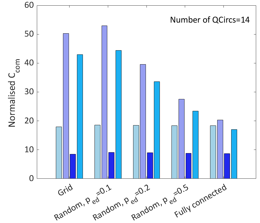
(a)

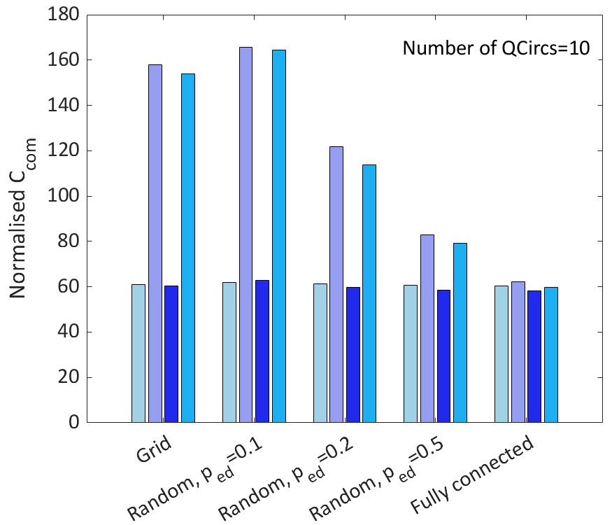
(b)

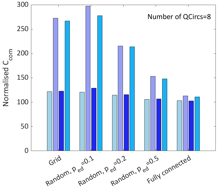
(c)

(d)

Figure 5: Comparison of proposed and benchmark QPU allocation methods based on the normalised $C_{\rm com}$ across various network scenarios and topologies. Three main cases are considered for the value of $M$ and the width of each QCirc: 1) $M=14$, $w_{m}\in\{15,\ldots,25\}$, 2) $M=10$, $w_{m}\in\{23,\ldots,33\}$, and 3) $M=8$, $w_{m}\in\{30,\ldots,40\}$.

(a)

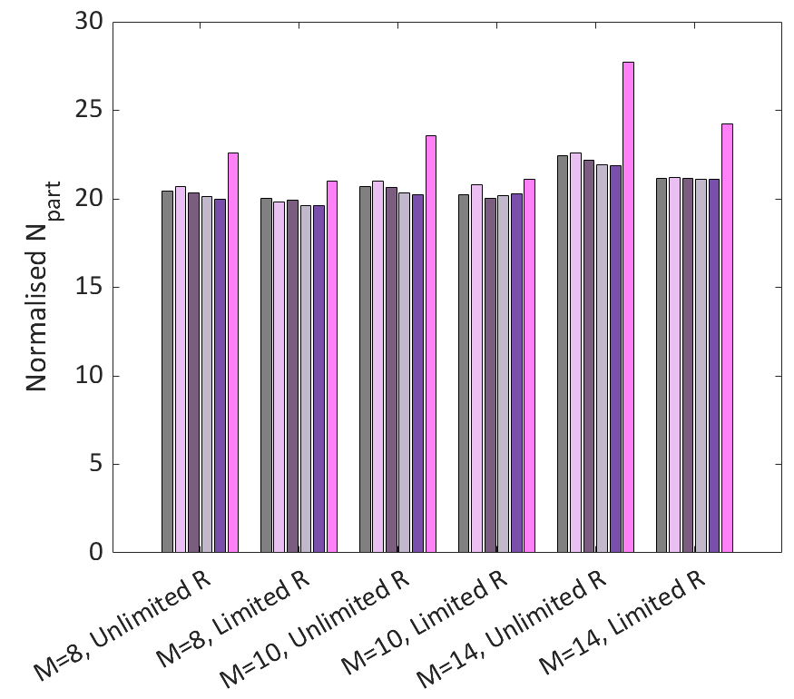
(b)

(c)

Figure 6: Performance comparison of the proposed and benchmark QPU allocation methods across various network scenarios and topologies. Three main cases are considered for the value of $M$ and the width of each QCirc: 1) $M=14$, $w_{m}\in\{15,\ldots,25\}$, 2) $M=10$, $w_{m}\in\{23,\ldots,33\}$, and 3) $M=8$, $w_{m}\in\{30,\ldots,40\}$. (a) Normalised $N_{\rm rgate}$. (b) Normalised $N_{\rm part}$.

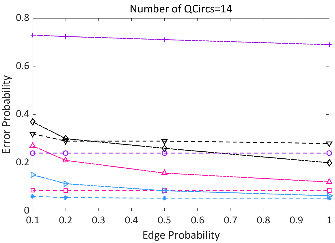
(a)

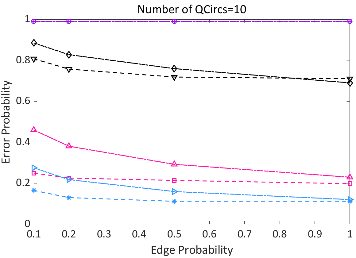
(b)

(c)

(d)

Figure 7: Error probability as a function of edge probability for random graph topologies and different quantum circuit types, assuming single circuit partition per QPU ($R=1$). Three main cases are considered for the value of $M$ and the width of each QCirc: 1) $M=14$, $w_{m}\in\{15,\ldots,25\}$, 2) $M=10$, $w_{m}\in\{23,\ldots,33\}$, and 3) $M=8$, $w_{m}\in\{30,\ldots,40\}$.

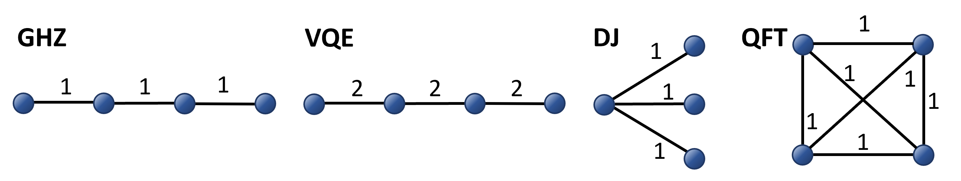
Figure 8: Graph representation of different QCirc types for a circuit width of $w=4$.

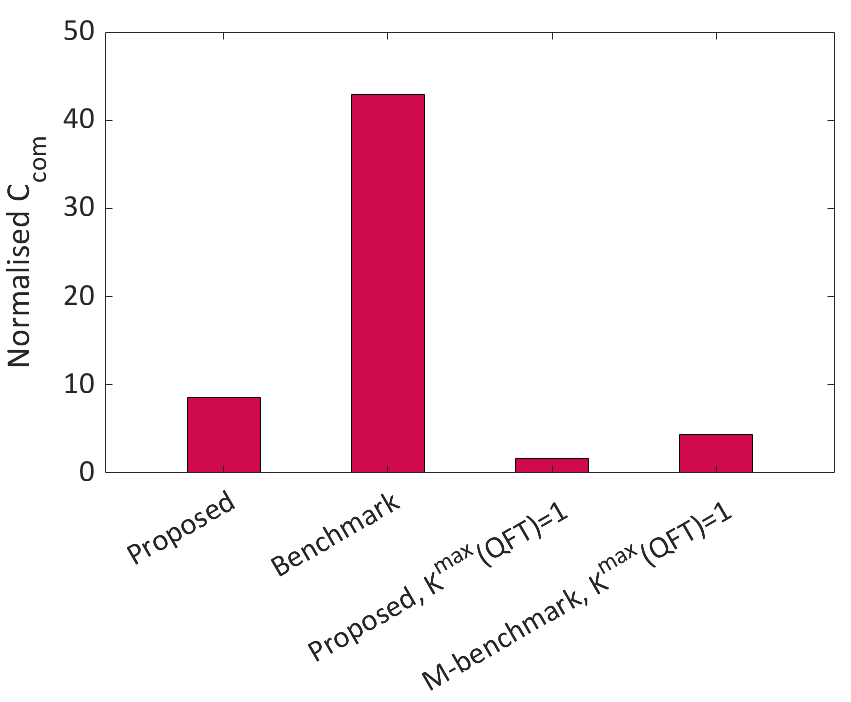
(a)

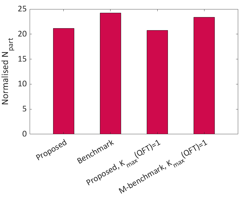
(b)

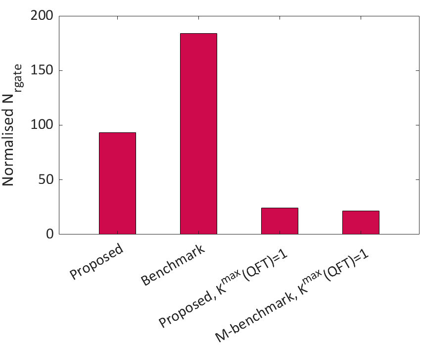
(c)

Figure 9: Comparison of proposed and benchmark QPU allocation methods, considering the specific case where the number of partitions is limited to one for the QFT circuit. A scenario with Limited R, $M=14$, and Grid topology is assumed. (a) Normalised $C_{\rm com}$ (b) Normalised $N_{\rm part}$ (b) Normalised $N_{\rm rgate}$.

Lastly, we evaluate the performance of the proposed method when the number of partitions for highly-connected QCircs is restricted. To this end, we consider the specific case where the number of partitions is limited to one ($K^{\rm max}=1$) for the QFT circuit, which is the QCirc with the largest connectivity parameter, $\nu$, among the four quantum circuits used in our simulations. The remaining three QCircs have no restrictions on their partition count. We focus on the scenario of Limited R, $M=14$, and Grid topology. For a fair comparison, the benchmark method is modified to accommodate this limitation. Specifically, QFT circuits are only assigned to QPUs with capacities exceeding their circuit widths. This modified version is referred to as “M-benchmark”.

Our simulation results show that imposing the $K^{\rm max}=1$ constraint on QFT circuits leads to a decrease in the assignment ratio, $r_{\rm asg}$, from 0.917 to 0.871 for the proposed method and from 0.806 to 0.775 for the benchmark method. This decrease is expected, as the imposed restriction prevents the assignment of a portion of QFT circuits in the batch. Nonetheless, the proposed method still outperforms the benchmark method.

Figure 9 illustrates $C_{\rm com}$, $N_{\rm part}$, and $N_{\rm rgate}$, normalised by $r_{\rm asg}$. The results clearly demonstrate that the proposed method surpasses the benchmark method in terms of inter-QPU communication cost and the number of circuit partitions. The normalised average number of remote gates is slightly higher for the proposed method compared to the benchmark, which can be attributed to the lower assignment of QFT circuits in the latter. Comparing the proposed method with and without the limitation on $K^{\rm max}$, we observe that the normalised inter-QPU communication cost is reduced by around $80\%$, while the assignment ratio decreases by only $5\%$. This highlights the trade-off between these two parameters. The network controller can intelligently explore and consider this trade-off to determine whether limiting $K^{\rm max}$ is beneficial in specific scenarios.

VI Conclusion

In this work, we addressed the challenge of efficient QPU allocation and QCirc scheduling in DQC networks. We proposed a multi-objective optimisation algorithm for QPU allocation that minimises the impact of inter-QPU communication latencies while maximising the number of assigned QCircs. The proposed optimisation algorithm considers the topology of the quantum network, link latencies, the properties and limitations of the QPUs, and the inherent features of the QCircs to effectively assign resources. We evaluated the proposed algorithm using various simulations. Our Results demonstrate that the proposed method efficiently allocates computing resources, enabling faster and more accurate execution of quantum circuits. In addition to our novel QPU allocation algorithm, we present an efficient QCirc scheduling model that seamlessly complements the allocation strategy.

In this work, we primarily focused on DQC networks that leverage both quantum and classical channels to generate entanglement between QPUs. However, alternative quantum computational techniques, such as circuit knitting, has been proposed in the literature, that require only classical channels for communication between QPUs [29, 30]. One exciting future research direction is to explore QPU allocation strategies for DQC networks that either employ solely classical channels or utilise both techniques. Another potential area of investigation is the integration of QPU allocation with advanced quantum compilation techniques, such as the noise-adaptive compilation method proposed in [5].

In summary, the findings and methodologies presented in this paper lay the foundation for the development of comprehensive execution management frameworks tailored to the unique challenges of DQC environments.

References

- [1] A. Yimsiriwattana et al., “Distributed quantum computing: A distributed shor algorithm,” vol. 5436. SPIE, 2004, pp. 360–372.
- [2] D. Cuomo, M. Caleffi, and A. S. Cacciapuoti, “Towards a distributed quantum computing ecosystem,” IET Quantum Communication, vol. 1, no. 1, pp. 3–8, 2020.
- [3] M. Caleffi et al., “Distributed quantum computing: a survey,” arXiv preprint arXiv:2212.10609, 2022.
- [4] J. Ang et al., “Architectures for multinode superconducting quantum computers,” arXiv preprint arXiv:2212.06167, 2022.
- [5] Y. Shi, P. Gokhale, P. Murali, J. M. Baker, C. Duckering, Y. Ding, N. C. Brown, C. Chamberland, A. Javadi-Abhari, A. W. Cross et al., “Resource-efficient quantum computing by breaking abstractions,” Proceedings of the IEEE, vol. 108, no. 8, pp. 1353–1370, 2020.
- [6] M. Maronese, L. Moro, L. Rocutto, and E. Prati, “Quantum compiling,” in Quantum Computing Environments. Springer, 2022, pp. 39–74.
- [7] R. D. Oliveira, S. Bahrani, E. Arabul, R. Wang, R. Nejabati, and D. Simeonidou, “FPGA-based deterministic and low-latency control for distributed quantum computing,” in IEEE INFOCOM 2023-IEEE Conference on Computer Communications Workshops (INFOCOM WKSHPS). IEEE, 2023, pp. 1–6.
- [8] D. Ferrari, A. S. Cacciapuoti, M. Amoretti, and M. Caleffi, “Compiler design for distributed quantum computing,” IEEE Transactions on Quantum Engineering, vol. 2, pp. 1–20, 2021.
- [9] D. Cuomo, M. Caleffi, K. Krsulich, F. Tramonto, G. Agliardi, E. Prati, and A. S. Cacciapuoti, “Optimized compiler for distributed quantum computing,” ACM Transactions on Quantum Computing, vol. 4, no. 2, pp. 1–29, 2023.
- [10] D. Ferrari, S. Carretta, and M. Amoretti, “A modular quantum compilation framework for distributed quantum computing,” IEEE Transactions on Quantum Engineering, 2023.
- [11] O. Daei et al., “Optimized quantum circuit partitioning,” International Journal of Theoretical Physics, vol. 59, no. 12, pp. 3804–3820, 2020.
- [12] W. Cambiucci et al., “Hypergraphic partitioning of quantum circuits for distributed quantum computing,” arXiv preprint arXiv:2301.05759, 2023.
- [13] P. Andres-Martinez et al., “Automated distribution of quantum circuits via hypergraph partitioning,” Physical Review A, vol. 100, no. 3, p. 032308, 2019.
- [14] Z. Davarzani, M. Zomorodi-Moghadam, M. Houshmand, and M. Nouri-Baygi, “A dynamic programming approach for distributing quantum circuits by bipartite graphs,” Quantum Information Processing, vol. 19, pp. 1–18, 2020.
- [15] D. Dadkhah, M. Zomorodi, and S. E. Hosseini, “A new approach for optimization of distributed quantum circuits,” International Journal of Theoretical Physics, vol. 60, pp. 3271–3285, 2021.
- [16] P. Andres-Martinez, T. Forrer, D. Mills, J.-Y. Wu, L. Henaut, K. Yamamoto, M. Murao, and R. Duncan, “Distributing circuits over heterogeneous, modular quantum computing network architectures,” arXiv preprint arXiv:2305.14148, 2023.
- [17] R. Parekh et al., “Quantum algorithms and simulation for parallel and distributed quantum computing,” in 2021 IEEE/ACM Second International Workshop on Quantum Computing Software (QCS). IEEE, 2021, pp. 9–19.
- [18] R. Yu, R. Dutta, and J. Liu, “On topology design for the quantum internet,” IEEE Network, vol. 36, no. 5, pp. 64–70, 2022.
- [19] M. Pant, H. Krovi, D. Towsley, L. Tassiulas, L. Jiang, P. Basu, D. Englund, and S. Guha, “Routing entanglement in the quantum internet,” npj Quantum Information, vol. 5, no. 1, p. 25, 2019.
- [20] K. Georgopoulos, C. Emary, and P. Zuliani, “Modeling and simulating the noisy behavior of near-term quantum computers,” Physical Review A, vol. 104, no. 6, p. 062432, 2021.
- [21] M. A. Nielsen and I. Chuang, “Quantum computation and quantum information,” 2002.
- [22] P. Belotti, C. Kirches, S. Leyffer, J. Linderoth, J. Luedtke, and A. Mahajan, “Mixed-integer nonlinear optimization,” Acta Numerica, vol. 22, pp. 1–131, 2013.
- [23] Y. Haimes, “On a bicriterion formulation of the problems of integrated system identification and system optimization,” IEEE transactions on systems, man, and cybernetics, no. 3, pp. 296–297, 1971.
- [24] P. Erdos, A. Rényi et al., “On the evolution of random graphs,” Publ. math. inst. hung. acad. sci, vol. 5, no. 1, pp. 17–60, 1960.
- [25] A. Hagberg, P. J. Swart, and D. A. Schult, “Exploring network structure, dynamics, and function using networkx,” in Proceedings of the 7th Python in Science Conference, 2008.
- [26] A. P. Place, L. V. Rodgers, P. Mundada, B. M. Smitham, M. Fitzpatrick, Z. Leng, A. Premkumar, J. Bryon, A. Vrajitoarea, S. Sussman et al., “New material platform for superconducting transmon qubits with coherence times exceeding 0.3 milliseconds,” Nature communications, vol. 12, no. 1, p. 1779, 2021.
- [27] M. Kjaergaard, M. E. Schwartz, J. Braumüller, P. Krantz, J. I.-J. Wang, S. Gustavsson, and W. D. Oliver, “Superconducting qubits: Current state of play,” Annual Review of Condensed Matter Physics, vol. 11, pp. 369–395, 2020.
- [28] N. Quetschlich, L. Burgholzer, and R. Wille, “MQT Bench: Benchmarking software and design automation tools for quantum computing,” Quantum, 2023, MQT Bench is available at https://www.cda.cit.tum.de/mqtbench/.
- [29] W. Tang, T. Tomesh, M. Suchara, J. Larson, and M. Martonosi, “Cutqc: using small quantum computers for large quantum circuit evaluations,” in Proceedings of the 26th ACM International conference on architectural support for programming languages and operating systems, 2021, pp. 473–486.
- [30] W. Tang and M. Martonosi, “Scaleqc: A scalable framework for hybrid computation on quantum and classical processors,” arXiv preprint arXiv:2207.00933, 2022.