Well-balanced Point-Average-Moment PolynomiAl-interpreted (PAMPA) Methods for Shallow Water Equations on Triangular Meshes

Abstract

In this paper, we develop novel well-balanced Point-Average-Moment PolynomiAl-interpreted (PAMPA) numerical methods for solving the two-dimensional shallow water equations on triangular meshes. The proposed PAMPA methods use a globally continuous representation of the variables, with degree of freedoms (DoFs) consisting of point values on the edges and average values within each triangular element. The update of cell averages is carried out using a conservative form of the partial differential equations (PDEs), while the point values are updated using a non-conservative formulation. This non-conservative formulation can be expressed in terms of either conservative or primitive variables. This new class of schemes is proved to be well-balanced and positivity-preserving. We validate the performance of the proposed methods through a series of numerical experiments. The numerical results are as expected and confirm that the performance of the PAMPA method using primitive variables in the non-conservative formulation is comparable to that using only the conservative variables. This work represents a step forward in the development and application of PAMPA methods for solving hyperbolic balance laws.

76M10, 76M12, 65M08, 35L40

1 Introduction

This paper is concerned with introducing novel well-balanced Point-Average-Moment PolynomiAl-interpreted (PAMPA) methods for solving the two-dimensional (2-D) Saint-Venant system of shallow water equations on general unstructured triangular meshes [15]:

(1) $$\left\{\begin{aligned} &h_{t}+(hu)_{x}+(hv)_{y}=0,\\ &(hu)_{t}+\left(hu^{2}+\frac{g}{2}h^{2}\right)_{x}+(huv)_{y}=-ghZ_{x},\\ &(hv)_{t}+(huv)_{x}+\left(hv^{2}+\frac{g}{2}h^{2}\right)_{y}=-ghZ_{y},\end{aligned}\right.$$

where $t$ is the time, $x$ and $y$ are the horizontal spatial coordinates. $h(x,y,t)$ represents the water depth above the bottom topography, denoted by $Z(x,y)$. $u(x,y,t)$ and $v(x,y,t)$ are the $x$- and $y$-components of the flow velocity, and $g$ is the gravitational constant. This system is widely used in many scientific and engineering applications related to modelling of water flows in rivers, lakes, and coastal areas.

The system (1) is a hyperbolic system of balance laws. The development of robust and accurate numerical methods for the computation of its solutions is both important and challenging as this nonlinear hyperbolic system admits both smooth and nonsmooth solutions: shocks, rarefaction waves, and their interactions. Additionally, in many real applications, quasi steady-state solutions must often be computed using a (practically affordable) coarse grid. In such situations, small perturbations of steady states may be amplified by the numerical schemes and the appearance of unphysical waves of magnitude proportional to the grid size may become larger than the magnitude of the waves to be captured (the so-called “numerical storm”); see, e.g., [25, 30, 35]. In order to prevent this, the developed numerical method should be well-balanced (WB), meaning it is capable of exactly balancing the flux and source terms to preserve relevant steady states within the machine accuracy, for instance, the “lake at rest” equilibria:

(2) $$u=v\equiv 0,\quad w:=h+Z\equiv{\rm Const.},$$

where $w$ denotes the water surface level.

In the past two decades, a number of WB methods for numerically solving the system (1) have been proposed; see, e.g., [17, 40, 37, 34, 42, 41, 10, 32, 13, 29, 7, 9, 11, 21, 39, 36, 33, 28, 22, 12]. Most of these methods are based on a discontinuous representation of the solution, either within the finite volume framework or more generally, in the context of discontinuous Galerkin methods. In contrast, this work assumes that the solution is globally continuous, and as in the active flux method [8, 18, 19, 20, 24], described by a combination of point values and average values. Unlike the “classical” active flux method, which relies on the method of characteristics for time evolution, the proposed active flux-like methods evolve the solution in time by standard Runge-Kutta methods, which are significantly simpler to implement in multidimensional cases. Another key difference is the flexibility of the proposed methods in updating point values, as they can employ several forms of the same system, such as the non-conservative forms written in terms of either conservative or primitive variables that will be shown in this work.

We focus on the active flux-like methods, which was originally introduced in [2] for the one-dimensional (1-D) Euler equations. This method uses two boundary point values and one average values per cell, constructs a quadratic polynomial approximation space that provides a formally third-order accurate approximation of the solution. In [3, 4], this method was extended to arbitrarily high-order case using either more point values from wider stencils or higher moments of conservative variables as additional DoFs. Very recently, the original third-order method and its high-order extension via higher moments were extended to 1-D hyperbolic system of balance laws, including the Saint Venant system in [6] and the system of blood flow in an artery [31]. In the multidimensional case, Abgrall et al. proposed an active flux-like method on triangular meshes for compressible flows in [5]. This method extends the work of [2] to several dimensions using simplex elements and deals with both conservative and non-conservative formulations of the same PDEs in terms of conservative variables.

In this paper, we extend the method in [5] developed for the hyperbolic conservation laws to solve the system of hyperbolic balance laws (1) and will name the resulting schemes well-balanced PAMPA (Point-Average-Moment PolynomiAl-interpreted). We introduce only third-order well-balanced PAMPA schemes in this work and plan to extend the construction to higher-order schemes via higher-moments in future works. For the third-order scheme, we use the cell average of the solution, which can also be viewed as the zero-th moment of the solution, as one degree of freedom (DoF) and others are the DoFs of the quadratic polynomials, which are all on the boundary of the elements. The time stepping relies on a standard Runge-Kutta time stepping, and several versions of the same problem can be used without preventing local conservation. More precisely, a conservative version of the studied PDEs is used to update the average values, while a non-conservative formulation, expressed in either conservative or primitive variables, is employed to evolve the point values. In the conservative formulation, the numerical flux is the continuous one, we can apply the divergence theorem and a Gauss-Lobatto quadrature with three points to evaluate integrals on each edge. To properly approximate the source terms and achieve the WB property, we start by rewriting these source terms in an equivalent form using the definition of the water surface level $w$. We then apply integration by parts to derive a numerical approximation that exactly balances the flux gradient at the steady state (2). In the non-conservative formulation, we use the LDA (Low Diffusion advection A) scheme [16] to compute the residuals for each DoF on the boundaries of the elements. To ensure the WB property in this context, we also incorporate the source terms into the residual distribution framework. Similar to the approach in [5], we implement a simple positivity-preserving mechanism based on a MOOD paradigm from [14, 38] and some first-order schemes to guarantee the resulting methods maintain the non-negativity of the water depth.

The rest of the paper is organized as follows. In Section 2, we introduce the novel third-order WB PAMPA methods. The low-order schemes, which will be used to retain the nonlinear stability, are described in Section 3. In Section 4, some numerical examples are presented to illustrate the high-order accuracy in smooth regions for general solutions, the good performance in simulating vortex propagation over flat and non-flat bottom topography, the WB property, and the robustness in capturing shocks and other complex wave patterns, of the proposed schemes. Finally, concluding remarks are given in Section 5.

2 Well-balanced third-order PAMPA schemes

In this section, we introduce the new third-order semi-discrete well-balanced PAMPA numerical schemes for solving the Saint-Venant system of shallow water equations (1) on triangular meshes. We first rewrite (1) in a vector form as follows:

(3) $$\frac{\partial\bm{u}}{\partial t}+{\rm div}~{}\bm{f}(\bm{u})=\bm{S}(\bm{u},Z),\quad\bm{u}=(h,hu,hv)^{\top},$$

where $\bm{u}\in\mathbb{R}^{d}$ with $d=2$ in this work, and

(4) $$\bm{f}(\bm{u})=\begin{pmatrix}h\bm{\nu}\\ h\bm{\nu}\bigotimes\bm{\nu}+p{\rm Id}_{d}\end{pmatrix},\quad\bm{S}(\bm{u},Z)=\begin{pmatrix}0\\ -gh\nabla Z\end{pmatrix}.$$

In (4), ${\rm Id}_{d}$ is the $d\times d$ identity matrix, $\bm{\nu}=(u,v)^{\top}$ represents the horizontal flow velocity vector, and the variable $p$ can be seen as the pressure, which for the shallow water equations takes the simple form $p=p(h)=\frac{g}{2}h^{2}$.

We note that for smooth solutions, (3) can be rewritten in a non-conservative form, either using the conservative variables $\bm{u}$:

(5) $$\frac{\partial\bm{u}}{\partial t}+\bm{J}\cdot\nabla\bm{u}=\bm{S}(\bm{u},Z),\quad\bm{J}\cdot\nabla\bm{u}=A\frac{\partial\bm{u}}{\partial x}+B\frac{\partial\bm{u}}{\partial y},$$

or using the primitive variables $\bm{v}=(h,u,v)^{\top}$:

(6) $$\frac{\partial\bm{v}}{\partial t}+\widetilde{\bm{J}}\cdot\nabla\bm{v}=\widetilde{\bm{S}}(Z),\quad\widetilde{\bm{J}}\cdot\nabla\bm{v}=\widetilde{A}\frac{\partial\bm{v}}{\partial x}+\widetilde{B}\frac{\partial\bm{v}}{\partial y},$$

where

$$\widetilde{\bm{S}}(Z)=\begin{pmatrix}0\\ -g\nabla Z\end{pmatrix}.$$

In (5), the matrices $A$ and $B$ are the Jacobians of the flux in the $x$- and $y$-directions with respect to $\bm{u}$:

$$A=\left(\begin{array}[]{ccc}0&1&0\\ gh-u^{2}&2u&0\\ -uv&v&u\\ \end{array}\right)\quad\mbox{and}\quad B=\left(\begin{array}[]{ccc}0&0&1\\ -uv&v&u\\ gh-v^{2}&0&2v\\ \end{array}\right).$$

In (6), the matrices $\widetilde{A}$ and $\widetilde{B}$ correspond to the coefficient matrices of the primitive formulation in the $x$- and $y$-directions:

$$\widetilde{A}=\left(\begin{array}[]{ccc}u&h&0\\ g&u&0\\ 0&0&u\\ \end{array}\right)\quad\mbox{and}\quad\widetilde{B}=\left(\begin{array}[]{ccc}v&0&h\\ 0&v&0\\ g&0&v\\ \end{array}\right).$$

The system is hyperbolic, i.e., for any vector $\bm{n}=(n_{x},n_{y})^{\top}$, the matrix

$$\bm{J}\cdot\bm{n}=An_{x}+Bn_{y}$$

or equivalently the matrix

$$\widetilde{\bm{J}}\cdot\bm{n}=\widetilde{A}n_{x}+\widetilde{B}n_{y}$$

is diagonalisable in $\mathbb{R}$.

Note that the conservative variable $\bm{u}\in\mathcal{D}_{\bm{u}}$, where

$$\mathcal{D}_{\bm{u}}=\{\bm{u}=(h,hu,hv)^{\top}\in\mathbb{R}^{3}:h>0\}.$$

It is easy to find a mapping $\Psi$, which is one-to-one and $C^{1}$ as well as invertible, so that the primitive variable $\bm{v}$ can be transformed from the conservative ones. Namely, $\bm{v}=\Psi(\bm{u})\in\mathcal{D}_{\bm{v}}$, where

$$\mathcal{D}_{\bm{v}}=\{\bm{v}=(h,u,v)^{\top}\in\mathbb{R}^{3}:h>0\}.$$

2.1 Approximation space

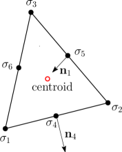
From now on, we assume that a triangulation $\mathcal{E}:=\bigcup\limits_{j}E_{j}$ of the computational domain, which consists of triangular cells $E_{j}$ of size $|E_{j}|$, is given. For each triangle $E$, the DoFs are defined at the three vertices $\sigma_{i}$ (for $i=1,2,3$), the three midpoints $\sigma_{i}$ (for $i=4,5,6$) on the three edges, and the cell average; see Figure 1. In this figure, we also define the normal vectors associated with each DoF, which will be used later. For any polynomial DoF $\sigma\in\{\sigma_{1},\sigma_{2},\ldots,\sigma_{6}\}$ over the element $E$:

• If $\sigma$ is a vertex, $\bm{n}_{\sigma}$ is the inward normal vector to the edge opposite to $\sigma$. For example, $\bm{n}_{1}$.

• If $\sigma$ is a midpoint, $\bm{n}_{\sigma}$ is the outward normal vector to the edge on which $\sigma$ is sitting. For example, $\bm{n}_{4}$.

Figure 1: Quadratic triangular element.

Equipped with the information of all DoFs for each triangle $E$, as shown in [5, Section 2], we can construct a polynomial space $V$ that contains quadratic polynomials and also accommodates the cell average as an independent variable. The seven basis functions for this polynomial space, denoted by $\{\varphi_{i}\}_{i=1}^{7}$, are defined as:

$$\varphi_{1}=\lambda_{1}(2\lambda_{1}-1),\quad \varphi_{2}=\lambda_{2}(2\lambda_{2}-1),\quad \varphi_{3}=\lambda_{3}(2\lambda_{3}-1),$$

$$\varphi_{4}=4\lambda_{1}\lambda_{2}-20\lambda_{1}\lambda_{2}\lambda_{3},\quad \varphi_{5}=4\lambda_{2}\lambda_{3}-20\lambda_{1}\lambda_{2}\lambda_{3},\quad \varphi_{6}=4\lambda_{3}\lambda_{1}-20\lambda_{1}\lambda_{2}\lambda_{3},$$

$$\varphi_{7}=60\lambda_{1}\lambda_{2}\lambda_{3},$$

where $(\lambda_{1},\lambda_{2},\lambda_{3})$ are the barycentric coordinates. One can verify that these basis functions satisfy the following conditions:

$$\varphi_{i}(\sigma_{j})=\delta_{i}^{j}~{}\mbox{for}~{}1\leq i,j\leq 6,\quad\int_{E}\varphi_{i}(\bm{x}){\rm d}\bm{x}=0,~{}\mbox{for}~{}i=1,\ldots,6$$

and

$$\varphi_{7}(\sigma_{j})=0,~{}\mbox{for}~{}j=1,\ldots,6,\quad\int_{E}\varphi_{7}(\bm{x}){\rm d}\bm{x}=0.$$

Finally, in the third-order PAMPA method, we seek an approximation of the studied PDEs (1), still denoted by $\bm{u}$ with an abuse of notation, which belongs to the finite dimensional space $V$ and within each element $E$ can be approximated by

(7) $$\bm{u}|_{E}\approx\sum_{i=1}^{6}\bm{u}_{\sigma_{i}}\varphi_{i}+\hbox{\vbox{\hrule height=0.5pt\kern 1.72218pt\hbox{\kern-0.50003pt$\bm{u}$\kern 0.0pt}}}_{E}\varphi_{7},$$

where $\bm{u}_{\sigma}$ is the point value of the variable $\bm{u}$ at the element boundary DoF $\sigma$ and $\hbox{\vbox{\hrule height=0.5pt\kern 1.72218pt\hbox{\kern-0.50003pt$\bm{u}$\kern 0.0pt}}}_{E}$ is the cell average defined as:

$$\hbox{\vbox{\hrule height=0.5pt\kern 1.72218pt\hbox{\kern-0.50003pt$\bm{u}$\kern 0.0pt}}}_{E}=\frac{1}{|E|}\int_{E}\bm{u}(\bm{x}){\rm d}\bm{x}.$$

We project the bottom function $Z$ into the same space $V$, to obtain an approximation which is still denoted by $Z$, again with an abuse of notation.

2.2 Semi-discrete scheme for the update of cell average

In this subsection, we describe how to evolve in time the cell average using the high-order spatial discretization.

A semi-discrete scheme for (3)–(4) is a system of ODEs for the approximations of the cell average $\hbox{\vbox{\hrule height=0.5pt\kern 1.72218pt\hbox{\kern-0.50003pt$\bm{u}$\kern 0.0pt}}}_{E}$ on a triangle $E$:

(8) $$|E|\frac{{\rm d}\hbox{\vbox{\hrule height=0.5pt\kern 1.72218pt\hbox{\kern-0.50003pt$\bm{u}$\kern 0.0pt}}}_{E}}{{\rm d}t}+\oint_{\partial E}{\bm{f}}(\bm{u})\cdot\bm{n}\;{\rm d}\gamma=\int_{E}\bm{S}(\bm{u},Z){\rm d}\bm{x},$$

where $\bm{n}$ is the outward unit normal at almost each point on the boundary $\partial E$ and we have applied the divergence theorem to rewrite the integral of the flux function over the triangle $E$.

In the numerical simulations, the surface integral over $\partial E$ is computed using a quadrature formula on each edge. Specifically,

(9) $$\oint_{\partial E}{\bm{f}}(\bm{u})\cdot\bm{n}\;{\rm d}\gamma\approx\sum_{l=1}^{3}\int_{{\rm ed}_{l}^{E}}{\bm{f}}(\bm{u})\cdot\bm{n}_{l}^{E}\;{\rm d}\gamma\approx\sum_{l=1}^{3}\sum_{i=1}^{3}\omega_{i}\ell_{l}{\bm{f}}(\bm{u}_{\sigma_{i}})\cdot\bm{n}_{l}^{E},$$

where $\ell_{l}$ is the length of the $l$-th edge of triangle $E$, $\bm{n}_{l}^{E}$ is the outer unit normal to that edge, and $(\omega_{i},\sigma_{i})$ for $i=1,2,3$ are the three Gauss-Lobatto quadrature weights and points. Note that these quadrature point values correspond to the three DoFs $\bm{u}_{\sigma}$ on each edge.

The next step is to define an appropriate approximation for the source terms in (8). The WB property of the conservative formulation (3)–(4) is guaranteed if the discretized cell average of the source terms exactly balances the flux evaluation in (9) for the “lake at rest” steady states (2). The source terms of the momentum equations in (3)–(4) take the form:

(10) $$-g\int_{E}h\nabla Z{\rm d}\bm{x} =-g\int_{E}(w-Z)\nabla Z{\rm d}\bm{x}$$

$$=\int_{E}gZ\nabla Z{\rm d}\bm{x}-g\int_{E}w\nabla Z{\rm d}\bm{x}:=\bm{S}_{E}^{1}+\bm{S}_{E}^{2}.$$

We introduce two vector fields $(\frac{g}{2}Z^{2},0)$ and $(0,\frac{g}{2}Z^{2})$, and apply the divergence theorem to the first integral $\bm{S}_{E}^{1}$ in (10), resulting in:

(11) $$\bm{S}_{E}^{1} =\frac{g}{2}\oint_{\partial E}Z^{2}{\rm Id}_{d}\cdot\bm{n}{\rm d}\gamma\approx\frac{g}{2}\sum_{l=1}^{3}\int_{{\rm ed}_{l}^{E}}Z^{2}{\rm Id}_{d}\cdot\bm{n}_{l}^{E}{\rm d}\gamma$$

$$\approx\frac{g}{2}\sum_{l=1}^{3}\sum_{i=1}^{3}\omega_{i}\ell_{l}(Z(\sigma_{i}))^{2}{\rm Id}_{d}\cdot\bm{n}_{l}^{E},$$

where $(\omega_{i},\sigma_{i})$ are the Gauss-Lobatto quadrature pairs that used in the computation of surface integral in (9). For the second integral $\bm{S}_{E}^{2}$ in (10), we approximate $Z$ and $w$ using the expansions provided in (7) and obtain:

(12) $$Z\approx\sum_{i=1}^{6}Z_{\sigma_{i}}\varphi_{i}+\hbox{\vbox{\hrule height=0.5pt\kern 1.72218pt\hbox{\kern-0.50003pt$Z$\kern 0.0pt}}}_{E}\varphi_{7}\quad\mbox{and}\quad w\approx\sum_{i=1}^{6}w_{\sigma_{i}}\varphi_{i}+\hbox{\vbox{\hrule height=0.5pt\kern 1.72218pt\hbox{\kern-0.50003pt$w$\kern 0.0pt}}}_{E}\varphi_{7},$$

where $w_{\sigma_{i}}=h_{\sigma_{i}}+Z_{\sigma_{i}}$ and $\hbox{\vbox{\hrule height=0.5pt\kern 1.72218pt\hbox{\kern-0.50003pt$w$\kern 0.0pt}}}_{E}=\hbox{\vbox{\hrule height=0.5pt\kern 1.72218pt\hbox{\kern-0.50003pt$h$\kern 0.0pt}}}_{E}+\hbox{\vbox{\hrule height=0.5pt\kern 1.72218pt\hbox{\kern-0.50003pt$Z$\kern 0.0pt}}}_{E}$. Substituting (12) into $S_{E}^{2}$ gives:

(13) $$\bm{S}_{E}^{2} \approx-g\int_{E}\left\{\Big{(}\sum_{i=1}^{6}w_{\sigma_{i}}\varphi_{i}+\hbox{\vbox{\hrule height=0.5pt\kern 1.72218pt\hbox{\kern-0.50003pt$w$\kern 0.0pt}}}_{E}\varphi_{7}\Big{)}\nabla\Big{(}\sum_{i=1}^{6}Z_{\sigma_{i}}\varphi_{i}+\hbox{\vbox{\hrule height=0.5pt\kern 1.72218pt\hbox{\kern-0.50003pt$Z$\kern 0.0pt}}}_{E}\varphi_{7}\Big{)}\right\}{\rm d}\bm{x}$$

$$=-g\sum_{i,j=1}^{6}w_{\sigma_{i}}Z_{\sigma_{i}}\int_{E}\varphi_{i}\nabla\varphi_{j}\,{\rm d}\bm{x}-g\sum_{i=1}^{6}w_{\sigma_{i}}\hbox{\vbox{\hrule height=0.5pt\kern 1.72218pt\hbox{\kern-0.50003pt$Z$\kern 0.0pt}}}_{E}\int_{E}\varphi_{i}\nabla\varphi_{7}\,{\rm d}\bm{x}$$

$$\quad-g\sum_{i=1}^{6}\hbox{\vbox{\hrule height=0.5pt\kern 1.72218pt\hbox{\kern-0.50003pt$w$\kern 0.0pt}}}_{E}Z_{\sigma_{i}}\int_{E}\varphi_{7}\nabla\varphi_{i}\,{\rm d}\bm{x}-g\hbox{\vbox{\hrule height=0.5pt\kern 1.72218pt\hbox{\kern-0.50003pt$w$\kern 0.0pt}}}_{E}\hbox{\vbox{\hrule height=0.5pt\kern 1.72218pt\hbox{\kern-0.50003pt$Z$\kern 0.0pt}}}_{E}\int_{E}\varphi_{7}\nabla\varphi_{7}\,{\rm d}\bm{x}.$$

Since the basis functions $\{\varphi_{i}\}$ are provided in Section 2.1, we can exactly compute all the integrals $\int_{E}\varphi_{i}\nabla\varphi_{j}\,{\rm d}\bm{x}$. This allows $\bm{S}_{E}^{2}$ to be given explicitly. For saving space, we refer to Appendix A for more details.

2.3 Semi-discrete schemes for the update of point value

In this subsection, we describe how to evolve the boundary DoFs of each triangle $E$ in time using the non-conservative formulations (5) or (6).

2.3.1 Non-conservative form expressed by conservative variables

We begin by studying the high-order spatial discretization for the non-conservative form (5), which is expressed in terms of the conservative variables $\bm{u}$. Following the approach introduced in [5, Section 3.1], the evolution of the boundary DoF $\bm{u}_{\sigma}$ is carried out by the following semi-discrete form:

(14) $$\frac{{\rm d}\bm{u}_{\sigma}}{{\rm d}t}+\sum\limits_{E,\sigma\in E}\Phi_{\sigma}^{E}(\bm{u})=0,$$

where the residual $\Phi_{\sigma}^{E}(\bm{u})$ is defined as

(15) $$\Phi_{\sigma}^{E}(\bm{u})=N_{\sigma}\big{(}K_{\sigma}^{E}\big{)}^{+}\Big{(}\bm{J}(\bm{u}_{\sigma})\cdot\nabla\bm{u}(\sigma)+\bm{P}(\bm{u}_{\sigma})\cdot\nabla\widehat{\bm{Z}}(\sigma)\Big{)}.$$

Here, $\nabla\bm{u}(\sigma)$ and $\nabla\widehat{\bm{Z}}(\sigma)$ are computed by taking gradients of the polynomial expansions introduced in Section 2.1,

$$K_{\sigma}^{E}=\bm{J}(\bm{u}_{\sigma})\cdot\bm{n}_{\sigma}^{E},\quad\mbox{and}\quad N_{\sigma}^{-1}=\sum\limits_{E,\sigma\in E}\big{(}K_{\sigma}^{E}\big{)}^{+}.$$

In (15), we incorporate the source terms into the residual by defining a vector $\widehat{\bm{Z}}=(0,Z,0)^{\top}$ and taking

$$\bm{P}\cdot\nabla\widehat{\bm{Z}}=P_{1}\frac{\partial\widehat{\bm{Z}}}{\partial x}+P_{2}\frac{\partial\widehat{\bm{Z}}}{\partial y},$$

where

$$P_{1}=\left(\begin{array}[]{ccc}0&0&0\\ 0&gh&0\\ 0&0&0\\ \end{array}\right)\quad\mbox{and}\quad P_{2}=\left(\begin{array}[]{ccc}0&0&0\\ 0&0&0\\ 0&gh&0\\ \end{array}\right).$$

The idea behind (15) is to have an up-winding mechanism for stability and to ensure the consistency in the case that if we have a linear $\bm{u}$ and $Z$, i.e., with $\nabla\bm{u}$ and $\nabla\widehat{\bm{Z}}$ constants, we are able to recover

$$\sum\limits_{E,\sigma\in E}\Phi_{\sigma}^{E}=\bm{J}(\bm{u}_{\sigma})\cdot\nabla\bm{u}+\bm{P}(\bm{u}_{\sigma})\cdot\nabla\widehat{\bm{Z}}.$$

2.3.2 Non-conservative form expressed by primitive variables

Next, we investigate the high-order spatial discretization for the non-conservative form (6), which is expressed using the primitive variables $\bm{v}$. Similar to the approach outlined in Section 2.3.1, we evolve the boundary DoF $\bm{v}_{\sigma}$ by the following semi-discrete form

(16) $$\frac{{\rm d}\bm{v}_{\sigma}}{{\rm d}t}+\sum\limits_{E,\sigma\in E}\widetilde{\Phi}_{\sigma}^{E}(\bm{v})=0,$$

where the residual $\widetilde{\Phi}_{\sigma}^{E}(\bm{v})$ is defined as

(17) $$\widetilde{\Phi}_{\sigma}^{E}(\bm{v})=\widetilde{N}_{\sigma}\big{(}\widetilde{K}_{\sigma}^{E}\big{)}^{+}\Big{(}\widetilde{\bm{J}}(\bm{v}_{\sigma})\cdot\nabla\bm{v}(\sigma)+\widetilde{\bm{P}}(\bm{v}_{\sigma})\cdot\nabla\widehat{\bm{Z}}(\sigma)\Big{)}.$$

Here,

$$\widetilde{K}_{\sigma}^{E}=\widetilde{\bm{J}}(\bm{v}_{\sigma})\cdot\bm{n}_{\sigma}^{E}\quad\mbox{and}\quad\widetilde{N}_{\sigma}^{-1}=\sum\limits_{E,\sigma\in E}\big{(}\widetilde{K}_{\sigma}^{E}\big{)}^{+}.$$

In (17), we also incorporate the source terms into the residual with the definitions

$$\widetilde{P}_{1}=\left(\begin{array}[]{ccc}0&0&0\\ 0&g&0\\ 0&0&0\\ \end{array}\right)\quad\mbox{and}\quad\widetilde{P}_{2}=\left(\begin{array}[]{ccc}0&0&0\\ 0&0&0\\ 0&g&0\\ \end{array}\right),$$

so that

$$\widetilde{\bm{P}}\cdot\nabla\widehat{\bm{Z}}=\widetilde{P}_{1}\frac{\partial\widehat{\bm{Z}}}{\partial x}+\widetilde{P}_{2}\frac{\partial\widehat{\bm{Z}}}{\partial y}.$$

To complete the computation in (17), we need to evaluate $\nabla\bm{v}(\sigma)$. First, from the boundary DoFs $\bm{u}_{\sigma}$ and Section 2, we obtain the point values $\bm{v}_{\sigma}=\Psi(\bm{u}_{\sigma})$ on the boundaries of each triangle $E$. Then, using the polynomial expansion in (7), we compute the point value of $\bm{u}$ at the centroid, denote as $\bm{u}_{c}$:

$$\bm{u}_{c}=\frac{20}{9}\hbox{\vbox{\hrule height=0.5pt\kern 1.72218pt\hbox{\kern-0.50003pt$\bm{u}$\kern 0.0pt}}}_{E}-\frac{1}{9}\sum_{i=1}^{3}\bm{u}_{\sigma_{i}}-\frac{8}{27}\sum_{i=4}^{6}\bm{u}_{\sigma_{i}}.$$

Consequently, this allows us to determine the point value of the primitive variables at the centroid, $\bm{v}_{c}=\Psi(\bm{u}_{c})$. Using these point values ($\{\bm{v}_{\sigma_{i}}\}_{i=1}^{6}$ and $\bm{v}_{c}$), we construct the Lagrange polynomial space containing $\bm{v}_{c}$ as in Section 2.1. The basis functions are defined as follows:

$$\phi_{7}=27\lambda_{1}\lambda_{2}\lambda_{3},$$

$$\phi_{1}=\lambda_{1}(2\lambda_{1}-1)+\frac{1}{9}\phi_{7}, \phi_{2}=\lambda_{2}(2\lambda_{2}-1)+\frac{1}{9}\phi_{7}, \phi_{3}=\lambda_{3}(2\lambda_{3}-1)+\frac{1}{9}\phi_{7},$$

$$\phi_{4}=4\lambda_{1}\lambda_{2}-\frac{4}{9}\phi_{7}, \phi_{5}=4\lambda_{2}\lambda_{3}-\frac{4}{9}\phi_{7}, \phi_{6}=4\lambda_{3}\lambda_{1}-\frac{4}{9}\phi_{7},$$

where these functions are constructed to satisfy the condition $\phi_{i}(\sigma_{j})=\delta_{i}^{j}$ for $1\leq i,j\leq 7$. Here, we represent the DoF at the centroid by $\sigma_{7}$. Finally, to evaluate $\nabla\bm{v}(\sigma)$, we take the gradient of the following approximation for $\bm{v}$:

$$\bm{v}=\sum_{i=1}^{6}\bm{v}_{\sigma_{i}}\phi_{i}+\bm{v}_{c}\phi_{7}.$$

2.4 Summary of the third-order well-balanced schemes

The proposed third-order WB PAMPA methods for the shallow water equations (1) are detailed in Eq. 4 and Eq. 5. The evolution of the cell averages is governed by (8), where the surface flux are defined in (9), and the approximations for the source terms are provided in (10), (11), and (13). The boundary point values are updated according to (14)–(15) for the conservative variables $\bm{u}$, or (16)–(17) for the primitive variables $\bm{v}$. The construction of the numerical schemes demonstrates that the PAMPA methods use a compact stencil and require fewer DoFs to achieve high order, offering potential advantages over WENO or DG methods. Moreover, the well-balanced property of the PAMPA methods is achieved without relying on complex numerical flux evaluations or hydrostatic reconstruction techniques. This advantage benefits from the continuous assumption of the solution and the natural well-balanced evolution of the point values. Finally, by collecting the results of the previous subsections, it is straightforward to prove the following WB result:

Proposition 1.

The third-order WB PAMPA methods for the shallow water equations (1), as described above, maintain the WB property for the steady states (2). That is, if the discrete data satisfy:

(18) $$u_{\sigma}=v_{\sigma}\equiv 0,\quad h_{\sigma}+Z_{\sigma}=\widehat{w}\equiv{\rm Const.},\quad\forall\sigma,$$

$$\hbox{\vbox{\hrule height=0.5pt\kern 1.72218pt\hbox{\kern-0.50003pt$(hu)$\kern 0.0pt}}}_{E}=\hbox{\vbox{\hrule height=0.5pt\kern 1.72218pt\hbox{\kern-0.50003pt$(hv)$\kern 0.0pt}}}_{E}\equiv 0,\quad \hbox{\vbox{\hrule height=0.5pt\kern 1.72218pt\hbox{\kern-0.50003pt$h$\kern 0.0pt}}}_{E}+\hbox{\vbox{\hrule height=0.5pt\kern 1.72218pt\hbox{\kern-0.50003pt$Z$\kern 0.0pt}}}_{E}=\widehat{w}\equiv{\rm Const.},\quad\forall E,$$

then (8), (14), and (16) reduce to

$$\frac{{\rm d}\hbox{\vbox{\hrule height=0.5pt\kern 1.72218pt\hbox{\kern-0.50003pt$\bm{u}$\kern 0.0pt}}}_{E}}{{\rm d}t}=0,\quad\frac{{\rm d}{\bm{u}}_{\sigma}}{{\rm d}t}=0,\quad\mbox{and}\quad\frac{{\rm d}{\bm{v}}_{\sigma}}{{\rm d}t}=0.$$

Proof 2.1.

We begin with the conservative formulation given in (8). When the data satisfy (18), for the mass equation, the source term is zero and the surface integral is also zero, since the velocity vector $\bm{\nu}_{\sigma}=0$ for all $\sigma$. For the momentum equations, which contain source terms, from (9) and (11) we obtain

$$\oint_{\partial E}{\bm{f}}(\bm{u})\cdot\bm{n}\;{\rm d}\gamma-\bm{S}_{E}^{1}=\frac{g}{2}\sum_{l=1}^{3}\sum_{i=1}^{3}\omega_{i}\ell_{l}[(h_{\sigma_{i}})^{2}-(Z_{\sigma_{i}})^{2}]{\rm Id}_{d}\cdot\bm{n}_{l}^{E}$$

$$=\frac{g}{12}\widehat{w}\Big{[}(h_{\sigma_{1}}-Z_{\sigma_{1}})\bm{n}_{1}+(h_{\sigma_{2}}-Z_{\sigma_{2}})\bm{n}_{2}+(h_{\sigma_{3}}-Z_{\sigma_{3}})\bm{n}_{3}\Big{]}$$

$$\quad-\frac{g}{3}\widehat{w}\Big{[}(h_{\sigma_{4}}-Z_{\sigma_{4}})\bm{n}_{3}+(h_{\sigma_{5}}-Z_{\sigma_{5}})\bm{n}_{1}+(h_{\sigma_{6}}-Z_{\sigma_{6}})\bm{n}_{2}\Big{]}.$$

Simultaneously, from (13) and Appendix A we obtain

$$\bm{S}_{E}^{2}=-\frac{g}{6}\widehat{w}\Big{[}Z_{\sigma_{1}}\bm{n}_{1}+Z_{\sigma_{2}}\bm{n}_{2}+Z_{\sigma_{3}}\bm{n}_{3}-4\big{(}Z_{\sigma_{4}}\bm{n}_{3}+Z_{\sigma_{5}}\bm{n}_{1}+Z_{\sigma_{6}}\bm{n}_{2}\big{)}\Big{]}.$$

Combining these results, we get

$$\oint_{\partial E}{\bm{f}}(\bm{u})\cdot\bm{n}\;{\rm d}\gamma-\bm{S}_{E}^{1}-\bm{S}_{E}^{2}=\frac{g}{12}\widehat{w}\big{[}(h_{\sigma_{1}}+Z_{\sigma_{1}})\bm{n}_{1}+(h_{\sigma_{2}}+Z_{\sigma_{2}})\bm{n}_{2}+(h_{\sigma_{3}}+Z_{\sigma_{3}})\bm{n}_{3}\big{]}$$

$$\quad-\frac{g}{3}\widehat{w}\big{[}(h_{\sigma_{4}}+Z_{\sigma_{4}})\bm{n}_{3}+(h_{\sigma_{5}}+Z_{\sigma_{5}})\bm{n}_{1}+(h_{\sigma_{6}}+Z_{\sigma_{6}})\bm{n}_{2}\big{]}$$

$$\quad=-\frac{g}{4}\widehat{w}(\bm{n}_{1}+\bm{n}_{2}+\bm{n}_{3})=0,$$

which implies that $\frac{{\rm d}\hbox{\vbox{\hrule height=0.5pt\kern 1.20552pt\hbox{\kern-0.35002pt$\bm{u}$\kern 0.0pt}}}_{E}}{{\rm d}t}=0$.

When the non-conservative form (5) is considered, for the point values $\bm{u}_{\sigma}$, we have

$$\bm{J}(\bm{u}_{\sigma})\cdot\nabla\bm{u}(\sigma)+\bm{P}(\bm{u}_{\sigma})\cdot\nabla\widehat{\bm{Z}}(\sigma)=\left(\begin{array}[]{c}0\\ gh_{\sigma}\nabla(h(\sigma)+Z(\sigma))\end{array}\right)=\left(\begin{array}[]{c}0\\ gh_{\sigma}\nabla\widehat{w}\end{array}\right)=\bm{0},$$

and hence, from (15), $\Phi_{\sigma}^{E}(\bm{u})=0$, which implies that $\frac{{\rm d}{\bm{u}}_{\sigma}}{{\rm d}t}=0$.

When the non-conservative form (6) is considered, for the point values $\bm{v}_{\sigma}$, we have

$$\widetilde{\bm{J}}(\bm{v}_{\sigma})\cdot\nabla\bm{v}(\sigma)+\widetilde{\bm{P}}(\bm{v}_{\sigma})\cdot\nabla\widehat{\bm{Z}}(\sigma)=\left(\begin{array}[]{c}0\\ g\nabla(h(\sigma)+Z(\sigma))\end{array}\right)=\left(\begin{array}[]{c}0\\ g\nabla\widehat{w}\end{array}\right)=\bm{0},$$

and hence, from (17), $\widetilde{\Phi}_{\sigma}^{E}(\bm{v})=0$, which implies that $\frac{{\rm d}{\bm{v}}_{\sigma}}{{\rm d}t}=0$.

3 Non-linear stabilization and low-order schemes

As pointed out in [5], the proposed high-order schemes possess linear stability. However, when the solution develops discontinuities, the high-order schemes will be prone to numerical oscillations. Additionally, the high-order schemes cannot guarantee the preservation of water depth positivity. To prevent spurious oscillations and nonlinear instabilities which may lead to the crash of the code, we need some sort of nonlinear limiting. For this purpose, we employ a simplified version of the MOOD paradigm from [14, 38] combined with low-order schemes to ensure the nonlinear stability. The idea involves working with two schemes ranging from third-order to first-order, where the first-order scheme is designed to be positivity-preserving and oscillation-eliminating. For more details on the MOOD approach, refer to [5, Section 3.4]. In the following, we focus on describing the first-order schemes.

3.1 First-order scheme for cell average

For the evolution of the cell average $\hbox{\vbox{\hrule height=0.5pt\kern 1.72218pt\hbox{\kern-0.50003pt$\bm{u}$\kern 0.0pt}}}_{E}$, we simply take a standard finite volume numerical flux (so we do not use the boundary values). For instance, we use the local Lax-Friedrichs numerical flux, replacing (9) with

(19) $$\oint_{\partial E}{\bm{f}}(\bm{u})\cdot\bm{n}\;{\rm d}\gamma\approx\sum_{l=1}^{3}\ell_{l}\widehat{\bm{f}}(\hbox{\vbox{\hrule height=0.5pt\kern 1.72218pt\hbox{\kern-0.50003pt$\bm{u}$\kern 0.0pt}}}_{E},\hbox{\vbox{\hrule height=0.5pt\kern 1.72218pt\hbox{\kern-0.50003pt$\bm{u}$\kern 0.0pt}}}_{E^{\prime}};\bm{n}_{l}^{E}),$$

where $\hbox{\vbox{\hrule height=0.5pt\kern 1.72218pt\hbox{\kern-0.50003pt$\bm{u}$\kern 0.0pt}}}_{E^{\prime}}$ represents the cell average of the neighboring triangle that shares the $l$-th edge with triangle $E$. The numerical flux $\widehat{\bm{f}}$ is defined as

(20) $$\widehat{\bm{f}}(\bm{a}_{1},\bm{a}_{2};\bm{n})=\frac{1}{2}\Big{[}\bm{f}(\bm{a}_{1})\cdot\bm{n}+\bm{f}(\bm{a}_{2})\cdot\bm{n}-\alpha(\bm{a}_{2}-\bm{a}_{1})\Big{]},$$

where,

$$\alpha=\max\Big{(}|\bm{a}_{1}\cdot\bm{n}|+c(\bm{a}_{1}),|\bm{a}_{2}\cdot\bm{n}|+c(\bm{a}_{2})\Big{)},$$

with $c=\sqrt{gh}$ playing the role of the sound speed for gas dynamics. In addition to this modification of flux evaluation, we also replace the source terms approximation using the midpoint quadrature rule. That is, we compute

$$-g\int_{E}h\nabla Z{\rm d}\bm{x} \approx-g|E|\hbox{\vbox{\hrule height=0.5pt\kern 1.72218pt\hbox{\kern-0.50003pt$h$\kern 0.0pt}}}_{E}\nabla Z(\bm{x}_{c})$$

$$=g\hbox{\vbox{\hrule height=0.5pt\kern 1.72218pt\hbox{\kern-0.50003pt$h$\kern 0.0pt}}}_{E}\Big{[}\frac{2}{3}\big{(}Z_{\sigma_{4}}\bm{n}_{3}+Z_{\sigma_{5}}\bm{n}_{1}+Z_{\sigma_{6}}\bm{n}_{2}\big{)}-\frac{1}{6}\big{(}Z_{\sigma_{1}}\bm{n}_{1}+Z_{\sigma_{2}}\bm{n}_{2}+Z_{\sigma_{3}}\bm{n}_{3}\big{)}\Big{]}.$$

3.2 First-order scheme for point value

For the evolution of the boundary values $\bm{u}_{\sigma}$ or $\bm{v}_{\sigma}$, the first-order spatial descretization is more involved. Following the approach introduced in [5], we temporarily re-number the boundary nodes for the definition of sub-elements. Starting with a selected DoF, denoted as $b_{1}$, we list the other nodes in a counter-clockwise manner, creating the list $\{b_{1},\ldots,b_{6}\}$ of all boundary DoFs, with the centroid labeled as $b_{7}$. We then define six sub-elements, $\{T^{E}_{i}\}_{i=1}^{6}$, with vertices given by $T^{E}_{1}=\{b_{1},b_{7},b_{2}\}$, $T^{E}_{2}=\{b_{2},b_{7},b_{3}\}$, $T^{E}_{3}=\{b_{3},b_{7},b_{4}\}$, $T^{E}_{4}=\{b_{4},b_{7},b_{5}\}$, $T^{E}_{5}=\{b_{5},b_{7},b_{6}\}$, $T^{E}_{6}=\{b_{6},b_{7},b_{1}\}$. For each sub-elements $T^{E}_{i}$, we can also get the inward normals $\bm{n}_{b_{i}}$. For quadratic elements, and using back the original numbering, this is illustrated in Figure 2.

Figure 2: Geometry for the first-order scheme.

The boundary values $\bm{u}_{\sigma}$ are also updated using (14) in the first-order case, but with a modified $\Phi_{\sigma}^{E}$:

(21) $$\Phi_{\sigma}^{E}=\frac{1}{|C_{\sigma}|}\sum_{T^{E}_{i},\sigma\in T^{E}_{i}}\Phi_{\sigma}^{T^{E}_{i}}(\bm{u}).$$

The residuals for each sub-triangle $T_{i}^{E}$ will be defined the following, which is done to get monotone first-order residual distribution schemes, see [16, 1] for example. We use a version inspired by the local Lax-Friedrichs scheme:

(22) $$\Phi_{\sigma}^{T^{E}_{i}}=\frac{1}{3}\oint_{T^{E}_{i}}\big{(}\bm{J}(\bm{u})\cdot\nabla\bm{u}+\bm{P}(\bm{u})\cdot\nabla\widehat{\bm{Z}}\big{)}{\rm d}\bm{x}+\alpha_{T^{E}_{i}}\big{(}\bm{u}_{\sigma}-\hbox{\vbox{\hrule height=0.5pt\kern 1.72218pt\hbox{\kern-0.50003pt$\bm{u}$\kern 0.0pt}}}_{T^{E}_{i}}\big{)}$$

with

(23) $$\oint_{T^{E}_{i}}\big{(}\bm{J}(\bm{u})\cdot\nabla\bm{u}+\bm{P}(\bm{u})\cdot\nabla\widehat{\bm{Z}}\big{)}{\rm d}\bm{x}\approx|T^{E}_{i}|\big{[}\bm{J}(\hbox{\vbox{\hrule height=0.5pt\kern 1.72218pt\hbox{\kern-0.50003pt$\bm{u}$\kern 0.0pt}}}_{T^{E}_{i}})\nabla\bm{u}(\hbox{\vbox{\hrule height=0.5pt\kern 1.72218pt\hbox{\kern-0.50003pt$\bm{u}$\kern 0.0pt}}}_{T^{E}_{i}})+\bm{P}(\hbox{\vbox{\hrule height=0.5pt\kern 1.72218pt\hbox{\kern-0.50003pt$\bm{u}$\kern 0.0pt}}}_{T^{E}_{i}})\cdot\nabla\widehat{\bm{Z}}(\hbox{\vbox{\hrule height=0.5pt\kern 1.72218pt\hbox{\kern-0.50003pt$Z$\kern 0.0pt}}}_{T^{E}_{i}})\big{]},$$

where a $P^{1}$ approximation on $T^{E}_{i}$ is used and $\hbox{\vbox{\hrule height=0.5pt\kern 1.72218pt\hbox{\kern-0.50003pt$\bm{u}$\kern 0.0pt}}}_{T^{E}_{i}}$ (resp. $\hbox{\vbox{\hrule height=0.5pt\kern 1.72218pt\hbox{\kern-0.50003pt$Z$\kern 0.0pt}}}_{T^{E}_{i}}$) is the arithmetic average of the $\bm{u}$’s (resp. $Z$’s) at three vertices of $T^{E}_{i}$ (hence we use the average value here). Finally,

(24) $$\alpha_{T^{E}_{i}}=\max\limits_{\begin{subarray}{c}\sigma\in T^{E}_{i},\\ \bm{n}_{b_{i}}\text{normals of~{}}T^{E}_{i}\end{subarray}}\rho\big{(}\bm{J}(\bm{u}_{\sigma})\cdot\bm{n}_{b_{i}}\big{)},$$

where $\rho(B)$ is the spectral radius of the matrix $B$. We still need to define $|C_{\sigma}|$, which is the dual control volume associated with the DoF $\bm{u}_{\sigma}$. It is

(25) $$|C_{\sigma}|=\sum_{E,\sigma\in E}\sum_{T^{E}_{i},\sigma\in T^{E}_{i}}\frac{|T^{E}_{i}|}{3},$$

and after some simple calculations, we see that

$$|C_{\sigma}|=\sum_{E,\sigma\in E}\frac{|E|}{9}.$$

It is well-known that the local Lax-Friedrichs’ finite volume scheme, defined by (9) and (19)–(20), for evolving the cell average of water depth, is positivity-preserving under the standard Courant–Friedrichs–Lewy (CFL) condition with a CFL number of 1. We now demonstrate that the first-order scheme defined by (14) and (21)–(23) also preserves the positivity for the point values of water depth.

Proposition 2.

Under the CFL condition

$$\Delta t\leq\frac{|T^{E}_{i}|}{3\alpha_{T^{E}_{i}}},$$

where $\alpha_{T^{E}_{i}}$ is given by (24), if $\hbox{\vbox{\hrule height=0.5pt\kern 1.72218pt\hbox{\kern-0.50003pt$h$\kern 0.0pt}}}_{E}$ and $h_{\sigma}^{n}$ are non-negative for any $\sigma\in\{\sigma_{1},\sigma_{2},\ldots,\sigma_{6}\}$, then $h_{\sigma}^{n+1}$ will also be non-negative in the first-order scheme defined by (14), (21), (22), and (23).

Proof 3.1.

For the shallow water equations (1), to verify the positivity-preserving property, we need to consider only the update of water depth. From (14), (15), (21), (22), and (23), we have

$$h_{\sigma}^{n+1} =h_{\sigma}^{n}-\frac{\Delta t}{|C_{\sigma}|}\sum_{E,\sigma\in E}\sum_{T^{E}_{i},\sigma\in T^{E}_{i}}\Big{(}\frac{1}{6}\sum_{j\in\{i,i+1\}}((h\bm{\nu})_{b_{j}}-(h\bm{\nu})_{b_{7}})\bm{n}_{b_{j}}+\alpha_{T^{E}_{i}}(h_{\sigma}-\hbox{\vbox{\hrule height=0.5pt\kern 1.72218pt\hbox{\kern-0.50003pt$h$\kern 0.0pt}}}_{T^{E}_{i}})\Big{)}$$

$$=\Big{(}1-\frac{\Delta t}{|C_{\sigma}|}\sum_{E,\sigma\in E}\sum_{T^{E}_{i},\sigma\in T^{E}_{i}}\alpha_{T^{E}_{i}}\Big{)}h_{\sigma}$$

$$\quad+\frac{\Delta t}{|C_{\sigma}|}\sum_{E,\sigma\in E}\sum_{T^{E}_{i},\sigma\in T^{E}_{i}}\Big{(}\alpha_{T^{E}_{i}}\hbox{\vbox{\hrule height=0.5pt\kern 1.72218pt\hbox{\kern-0.50003pt$h$\kern 0.0pt}}}_{T^{E}_{i}}-\frac{1}{6}\sum_{j\in\{i,i+1\}}((h\bm{\nu})_{b_{j}}-(h\bm{\nu})_{b_{7}})\bm{n}_{b_{j}}\Big{)}.$$

Since $\Delta t\leq\frac{|T^{E}_{i}|}{3\alpha_{T^{E}_{i}}}$, it follows that

$$\Delta t\sum_{E,\sigma\in E}\sum_{T^{E}_{i},\sigma\in T^{E}_{i}}\alpha_{T^{E}_{i}}\leq\sum_{E,\sigma\in E}\sum_{T^{E}_{i},\sigma\in T^{E}_{i}}\frac{|T^{E}_{i}|}{3}.$$

Using the definition of $|C_{\sigma}|$ in (25), we obtain

$$\Delta t\sum_{E,\sigma\in E}\sum_{T^{E}_{i},\sigma\in T^{E}_{i}}\alpha_{T^{E}_{i}}\leq|C_{\sigma}|,$$

which implies that

$$1-\frac{\Delta t}{|C_{\sigma}|}\sum_{E,\sigma\in E}\sum_{T^{E}_{i},\sigma\in T^{E}_{i}}\alpha_{T^{E}_{i}}\geq 0.$$

Additionally, we have

$$\alpha_{T^{E}_{i}}\hbox{\vbox{\hrule height=0.5pt\kern 1.72218pt\hbox{\kern-0.50003pt$h$\kern 0.0pt}}}_{T^{E}_{i}}-\frac{1}{6}\sum_{j\in\{i,i+1\}}((h\bm{\nu})_{b_{j}}-(h\bm{\nu})_{b_{7}})\bm{n}_{b_{j}}\geq\alpha_{T^{E}_{i}}\hbox{\vbox{\hrule height=0.5pt\kern 1.72218pt\hbox{\kern-0.50003pt$h$\kern 0.0pt}}}_{T^{E}_{i}}-\frac{1}{6}\alpha_{T^{E}_{i}}(h_{b_{i}}+h_{b_{i+1}}+2h_{b_{7}})$$

$$\quad=\frac{1}{3}\alpha_{T^{E}_{i}}(h_{b_{i}}+h_{b_{i+1}}+h_{b_{7}})-\frac{1}{6}\alpha_{T^{E}_{i}}(h_{b_{i}}+h_{b_{i+1}}+2h_{b_{7}})$$

$$\quad=\frac{1}{6}\alpha_{T^{E}_{i}}(h_{b_{i}}+h_{b_{i+1}})\geq 0.$$

Combining the above results, we can conclude that $h_{\sigma}^{n+1}\geq 0$.

When considering the non-conservative form (6) for updating $\bm{v}_{\sigma}$, we replace (22) and (23) with

$$\Phi_{\sigma}^{T^{E}_{i}}=\frac{1}{3}\oint_{T^{E}_{i}}\big{(}\widetilde{\bm{J}}(\bm{v})\cdot\nabla\bm{v}+\widetilde{\bm{P}}(\bm{v})\cdot\nabla\widehat{\bm{Z}}\big{)}{\rm d}\bm{x}+\alpha_{T^{E}_{i}}\big{(}\bm{v}_{\sigma}-\hbox{\vbox{\hrule height=0.5pt\kern 1.72218pt\hbox{\kern-0.50003pt$\bm{v}$\kern 0.0pt}}}_{T^{E}_{i}}\big{)}$$

and

$$\oint_{T^{E}_{i}}\big{(}\widetilde{\bm{J}}(\bm{v})\cdot\nabla\bm{u}+\widetilde{\bm{P}}(\bm{v})\cdot\nabla\widehat{\bm{Z}}\big{)}{\rm d}\bm{x}\approx|T^{E}_{i}|\big{[}\widetilde{\bm{J}}(\hbox{\vbox{\hrule height=0.5pt\kern 1.72218pt\hbox{\kern-0.50003pt$\bm{v}$\kern 0.0pt}}}_{T^{E}_{i}})\nabla\bm{v}(\hbox{\vbox{\hrule height=0.5pt\kern 1.72218pt\hbox{\kern-0.50003pt$\bm{v}$\kern 0.0pt}}}_{T^{E}_{i}})+\widetilde{\bm{P}}(\hbox{\vbox{\hrule height=0.5pt\kern 1.72218pt\hbox{\kern-0.50003pt$\bm{v}$\kern 0.0pt}}}_{T^{E}_{i}})\cdot\nabla\widehat{\bm{Z}}(\hbox{\vbox{\hrule height=0.5pt\kern 1.72218pt\hbox{\kern-0.50003pt$Z$\kern 0.0pt}}}_{T^{E}_{i}})\big{]}.$$

A similar positivity-preserving analysis as in 2 can be performed for this case, but is omitted here for brevity.

4 Numerical examples

In this section, we demonstrate the performance of the proposed third-order WB PAMPA schemes on several numerical examples. For all the examples tested, the cell averages are updated using the conservative formulation (3), while the point values are evolved using the non-conservative formulations (5) or (6). We refer to the scheme designed for (3) and (5) as “PAMPA-$\bm{u}$” scheme, and the scheme designed for (3) and (6) as “PAMPA-$\bm{v}$” scheme. Numerical results obtained with these two schemes will be compared.

In all numerical experiments, the semi-discrete ODEs are integrated by the three-stage third-order strong stability preserving (SSP) Runge-Kutta method. Unless otherwise specified, the acceleration due to gravity is fixed as $g=9.812$ and zero-order extrapolation boundary conditions are used. All the meshes are unstructured and generated by GMSH [23].

Example 1—Accuracy Test

The goal of the first example is to experimentally check the high-order accuracy of the proposed schemes when applied to the following two-dimensional problem:

$$Z(r)=0.2e^{\frac{1-r^{2}}{2}},~{}h(r,0)=1-\frac{1}{4g}e^{2(1-r^{2})}-Z(r),~{}u(r,0)=ye^{1-r^{2}},~{}v(r,0)=-xe^{1-r^{2}},$$

where $r=\sqrt{x^{2}+y^{2}}$. The computational domain is $[-10,10]\times[-10,10]$. Note that this is a stationary equilibrium of the system (1) so that the exact solution coincides with the initial condition at any time.

We compute the numerical solution until the final time $t=1$ using both the PAMPA-$\bm{u}$ and PAMPA-$\bm{v}$ schemes. The unstructured meshes are obtained using the Frontal-Delaunay option with mesh characteristic lengthes $1.0$, $0.5$, $0.25$, and $0.125$. We measure the discrete $L^{1}$-errors for cell averages as well as the point values of the conservative variables and then compute the rate of convergence. Tables 1 and 2 report the results obtained by the PAMPA-$\bm{u}$ scheme, while Tables 3 and 4 reports those results obtained by the PAMPA-$\bm{v}$ scheme. From the presented results, we can see that the expected experimental third order of accuracy is achieved for both two studied PAMPA schemes.

Table 1: Example 1: $L^{1}$ errors and numerical orders of accuracy for cell averages using PAMPA-$\bm{u}$ scheme.

$\max\limits_{j}\sqrt{|E_{j}|}$	$h$	rate	$hu$	rate	$hv$	rate
$0.7510$	$1.581\times 10^{-4}$	-	$6.319\times 10^{-4}$	-	$7.490\times 10^{-4}$	-
$0.3681$	$3.402\times 10^{-5}$	$2.15$	$1.335\times 10^{-4}$	$2.18$	$1.282\times 10^{-4}$	$2.48$
$0.1954$	$5.811\times 10^{-6}$	$2.79$	$1.911\times 10^{-5}$	$3.07$	$1.915\times 10^{-5}$	$3.10$
$0.0937$	$8.450\times 10^{-7}$	$2.62$	$2.862\times 10^{-6}$	$2.58$	$2.853\times 10^{-6}$	$2.59$

Table 2: Example 1: Same as in Table 1 but for point values.

$\max\limits_{\sigma}\sqrt{|C_{\sigma}|}$	$h$	rate	$hu$	rate	$hv$	rate
$0.6128$	$1.123\times 10^{-4}$	-	$7.605\times 10^{-4}$	-	$8.153\times 10^{-4}$	-
$0.3025$	$2.345\times 10^{-5}$	$2.22$	$1.254\times 10^{-4}$	$2.55$	$1.269\times 10^{-4}$	$2.63$
$0.1552$	$3.915\times 10^{-6}$	$2.68$	$1.946\times 10^{-5}$	$2.79$	$1.964\times 10^{-5}$	$2.80$
$0.0755$	$5.676\times 10^{-7}$	$2.68$	$3.414\times 10^{-6}$	$2.42$	$3.421\times 10^{-6}$	$2.43$

Table 3: Example 1: $L^{1}$ errors and numerical orders of accuracy for cell averages using PAMPA-$\bm{v}$ scheme.

$\max\limits_{j}\sqrt{|E_{j}|}$	$h$	rate	$hu$	rate	$hv$	rate
$0.7510$	$1.611\times 10^{-4}$	-	$7.536\times 10^{-4}$	-	$8.059\times 10^{-4}$	-
$0.3681$	$3.840\times 10^{-5}$	$2.01$	$1.357\times 10^{-4}$	$2.40$	$1.410\times 10^{-4}$	$2.44$
$0.1954$	$6.431\times 10^{-6}$	$2.82$	$2.127\times 10^{-5}$	$2.93$	$2.139\times 10^{-5}$	$2.98$
$0.0937$	$9.427\times 10^{-7}$	$2.62$	$3.186\times 10^{-6}$	$2.58$	$3.187\times 10^{-6}$	$2.59$

Table 4: Example 1: Same as in Table 3 but for point values.

$\max\limits_{\sigma}\sqrt{|C_{\sigma}|}$	$h$	rate	$hu$	rate	$hv$	rate
$0.6128$	$1.165\times 10^{-4}$	-	$9.273\times 10^{-4}$	-	$9.091\times 10^{-4}$	-
$0.3025$	$2.634\times 10^{-5}$	$2.10$	$1.291\times 10^{-4}$	$2.79$	$1.336\times 10^{-4}$	$2.72$
$0.1552$	$4.332\times 10^{-6}$	$2.70$	$2.007\times 10^{-5}$	$2.79$	$2.004\times 10^{-5}$	$2.84$
$0.0755$	$6.330\times 10^{-7}$	$2.67$	$3.492\times 10^{-6}$	$2.43$	$3.483\times 10^{-6}$	$2.43$

Example 2—Traveling Vortex

In the second example, we consider a traveling vortex initially located at $(0,0)$ that propagates with a speed of $(1,\frac{\sqrt{2}}{2})$ in a square computational domain $[-10,10]\times[-10,10]$. The initial conditions are a slightly modification of those from the previous example and are given by

(26) $$h(r,0)=1-\frac{1}{4g}e^{2(1-r^{2})},~{}u(r,0)=1+ye^{1-r^{2}},~{}v(r,0)=\frac{\sqrt{2}}{2}-xe^{1-r^{2}},$$

where $r=\sqrt{x^{2}+y^{2}}$.

We first consider a flat bottom topography, i.e., $Z(x,y)=0$. In this case, the vortex travels in the direction $(1,\frac{\sqrt{2}}{2})$, and we can derive the exact solution, which is defined as

$$h(x,y,t)=h(x-t,y-\frac{\sqrt{2}}{2}t,0),$$

$$u(x,y,t)=u(x-t,y-\frac{\sqrt{2}}{2}t,0),$$

$$v(x,y,t)=v(x-t,y-\frac{\sqrt{2}}{2}t,0).$$

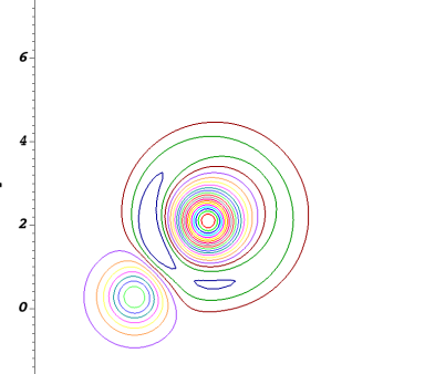
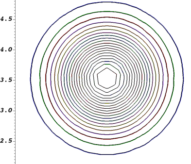
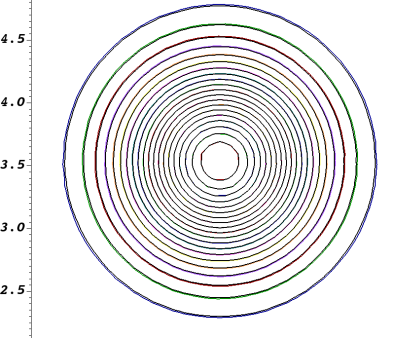
In Figure 3, we show the computed water depth $h$ and the exact solution (represented by the black curve, which coincides with the numerical solution) on a mesh with 23246 triangular elements and 46893 DoFs at the final time $t=5$. As one can observe, both two studied schemes can capture the traveling vortex very accurately. The vortex moves in the correct direction and reaches the right final position. Moreover, at this scale, the difference between the exact and numerical solutions is minimal.

(a) PAMPA-$\bm{u}$: $\hbox{\vbox{\hrule height=0.5pt\kern 1.37775pt\hbox{\kern-0.40002pt$h$\kern 0.0pt}}}_{E}$

(b) PAMPA-$\bm{u}$: $h_{\sigma}$

(c) PAMPA-$\bm{v}$: $\hbox{\vbox{\hrule height=0.5pt\kern 1.37775pt\hbox{\kern-0.40002pt$h$\kern 0.0pt}}}_{E}$

(d) PAMPA-$\bm{v}$: $h_{\sigma}$

Figure 3: Example 2: Cell averages and point values of water depth at $t=5$ computed by the PAMPA-$\bm{u}$ (top row) and PAMPA-$\bm{v}$ (bottom row) schemes.

Next, we introduce a non-flat bottom topography, defined as

$$Z(x,y)=0.2e^{\frac{1}{2}-2((x-2)^{2}+(y-2)^{2})},$$

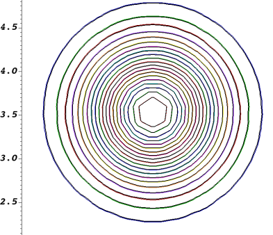
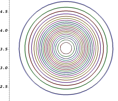
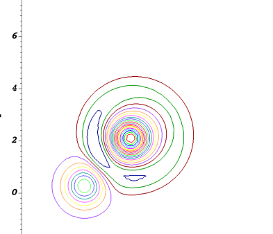
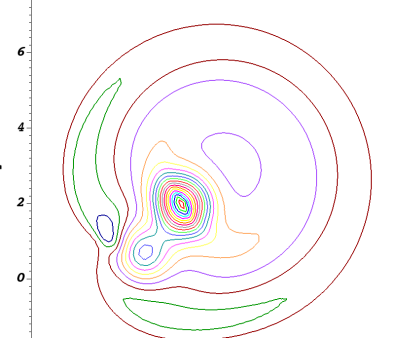
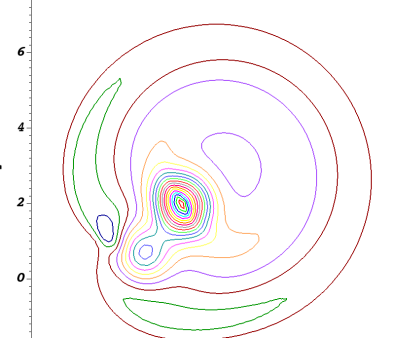
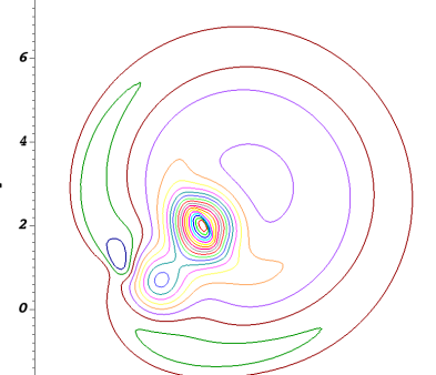
while keeping others the same as in (26). In this case, the water depth is perturbed due to the non-flat bottom, but the vortex still travels in the same direction. In Figure 4, we show the water depth at time $t=0.39$. At this moment, the front part of the vortex has just passed through the bottom topography and the tail part remains behind it. Figure 5 presents the water depth at time $t=1$, corresponding to the moment when the tail part of the vortex is about to pass over the bottom. From these results, we can conclude that both two studied schemes can accurately capture the dynamical traveling processes of the vortex over a non-flat bottom topography. This demonstrates great potential for applying these schemes to the study of rotating shallow water equations and the simulation of cyclonic vortices; see, e.g., [26, 27].

(a) PAMPA-$\bm{u}$: $\hbox{\vbox{\hrule height=0.5pt\kern 1.37775pt\hbox{\kern-0.40002pt$h$\kern 0.0pt}}}_{E}$

(b) PAMPA-$\bm{u}$: $h_{\sigma}$

(c) PAMPA-$\bm{v}$: $\hbox{\vbox{\hrule height=0.5pt\kern 1.37775pt\hbox{\kern-0.40002pt$h$\kern 0.0pt}}}_{E}$

(d) PAMPA-$\bm{v}$: $h_{\sigma}$

Figure 4: Example 2: Cell averages and point values of water depth at $t=0.39$ computed by the PAMPA-$\bm{u}$ (top row) and PAMPA-$\bm{v}$ (bottom row) schemes over non-flat bottom topography.

(a) PAMPA-$\bm{u}$: $\hbox{\vbox{\hrule height=0.5pt\kern 1.37775pt\hbox{\kern-0.40002pt$h$\kern 0.0pt}}}_{E}$

(b) PAMPA-$\bm{u}$: $h_{\sigma}$

(c) PAMPA-$\bm{v}$: $\hbox{\vbox{\hrule height=0.5pt\kern 1.37775pt\hbox{\kern-0.40002pt$h$\kern 0.0pt}}}_{E}$

(d) PAMPA-$\bm{v}$: $h_{\sigma}$

Figure 5: Example 2: Same as in Figure 4 but at time $t=1$.

Example 3—Well-balanced Test: Flows over Three Humps

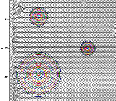
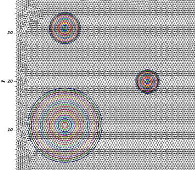
In the third example, we verify the WB property of the proposed two schemes towards the steady-state solution. The computational domain is $[0,40]\times[0,40]$ and the bottom topography is defined as:

$$Z(x,y)=\max\Big{(}0,1-\frac{1}{8}r_{10,11},1-\frac{3}{10}r_{10,31},1-\frac{4}{10}r_{27,20}\Big{)},$$

where $r_{a,b}=\sqrt{(x-a)^{2}+(y-b)^{2}}$. The initial data satisfy a lake at rest solution, that is,

$$h(x,y,0)=4-Z(x,y),\quad u(x,y,0)=v(x,y,0)\equiv 0.$$

We compute the solution until a final time $t=20$ on the triangular mesh consisting of $3718$ elements and $7597$ DoFs. In Figure 6, we present the results of water depth with 20 isolines obtained by the two studied schemes. We can see that the initial profile of water depth is preserved.

(a) PAMPA-$\bm{u}$: $\hbox{\vbox{\hrule height=0.5pt\kern 1.37775pt\hbox{\kern-0.40002pt$h$\kern 0.0pt}}}_{E}$

(b) PAMPA-$\bm{u}$: $h_{\sigma}$

(c) PAMPA-$\bm{v}$: $\hbox{\vbox{\hrule height=0.5pt\kern 1.37775pt\hbox{\kern-0.40002pt$h$\kern 0.0pt}}}_{E}$

(d) PAMPA-$\bm{v}$: $h_{\sigma}$

Figure 6: Example 3: Numerical solution (cell averages and point values of water depth) at $t=20$ computed by the PAMPA-$\bm{u}$ (top row) and PAMPA-$\bm{v}$ (bottom row) schemes.

Furthermore, in order to demonstrate that the lake at rest equilibria is indeed maintained up to round-off error, we compute the discrete $L^{1}$- and $L^{\infty}$-errors for the numerical solution (cell averages and point values of water depth $h$ and discharge $h\bm{\nu}$). We show the obtained results in Tables 5 and 6. As one can clearly see, all errors are within machine accuracy, which verifies the WB property of the proposed PAMPA schemes.

Table 5: Example 3: $L^{1}$- and $L^{\infty}$-errors for the lake at rest obtained by PAMPA-$\bm{u}$ scheme.

Var.	$h$		$hu$		$hv$
	$L^{1}$-error	$L^{\infty}$-error	$L^{1}$-error	$L^{\infty}$-error	$L^{1}$-error	$L^{\infty}$-error
$\bm{u}$	3.40e-16	6.22e-15	7.83e-14	1.37e-12	7.83e-14	1.48e-12
$\bm{u}_{\sigma}$	2.50e-16	9.77e-15	5.08e-14	2.67e-12	4.98e-14	2.45e-12

Table 6: Example 3: Same as in Table 5 but the errors are obtained by PAMPA-$\bm{v}$ scheme.

Var.	$h$		$hu$		$hv$
	$L^{1}$-error	$L^{\infty}$-error	$L^{1}$-error	$L^{\infty}$-error	$L^{1}$-error	$L^{\infty}$-error
$\bm{u}$	4.13e-16	1.07e-14	8.21e-14	4.75e-12	8.14e-14	4.55e-12
$\bm{u}_{\sigma}$	2.96e-16	1.78e-14	5.38e-14	9.54e-12	5.21e-14	6.29e-12

Example 4—Small Perturbation of a Steady-State Solution

In the fourth example, we perform an additional test to verify the WB property of the proposed schemes by imposing a perturbation into the stationary solution. Non well-balanced schemes often struggle to capture the correct propagation of a perturbation when its magnitude is smaller than the spatial discretization size. While mesh refinement can improve this issue, it is typically not a practically affordable solution. Therefore, well-balanced schemes are highly valuable. In what follows, we consider a non-flat bottom topography defined by

$$Z(x,y)=0.8e^{-50\big{(}(x-1)^{2}+(y-1)^{2}\big{)}},$$

prescribed in a computational domain $[0,2]\times[0,2]$. The initial conditions are given by

$$h(x,y,0)=1-Z(x,y)+10^{-4}e^{-20\big{(}(x-0.8)^{2}+(y-0.8)^{2}\big{)}},\quad u(x,y,0)=v(x,y,0)\equiv 0.$$

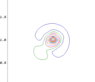
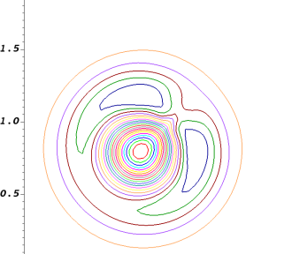
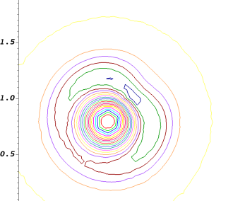
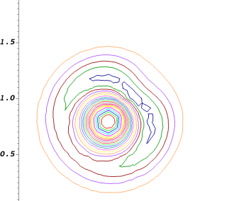
We compute the numerical results using the WB PAMPA-$\bm{u}$, WB PAMPA-$\bm{v}$, and non well-balanced schemes, and show the propagation of the perturbation in the cell averages of water depth $h$ at time $t=0.1$. Figure 7 shows the results obtained using a coarse mesh with 944 triangular elements and 1969 DoFs. We can clearly see that the PAMPA-$\bm{u}$ and PAMPA-$\bm{v}$ schemes produce highly similar results, while the non well-balanced scheme shows substantial differences.

(a) PAMPA-$\bm{u}$

(b) PAMPA-$\bm{v}$

(c) non WB

Figure 7: Example 4: Perturbation in the cell averages of water depth at $t=0.1$ computed by the PAMPA-$\bm{u}$ (left column), PAMPA-$\bm{v}$ (middle column), and non well-balanced (right column) schemes. A coarse mesh with 944 triangular elements and 1969 DoFs is used.

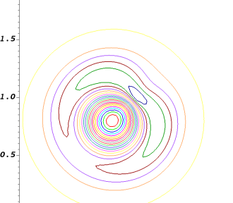
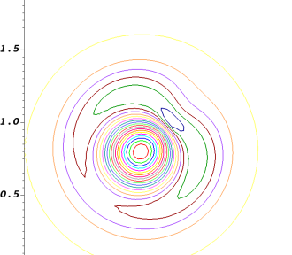
To further illustrate the effectiveness of WB schemes, we refine the mesh to 5824 elements and 11849 DoFs and plot the results in Figure 8. As one can observe, the result computed by the non well-balanced scheme now align more closely with those obtained using the WB schemes. For the WB schemes, the numerical solutions remain consistent between the coarse and fine meshes. This also demonstrate the ability of WB schemes to accurately capture small perturbations with lower computational cost.

(a) PAMPA-$\bm{u}$

(b) PAMPA-$\bm{v}$

(c) non WB

Figure 8: Example 4: Same as in Figure 7 but using a fine mesh with 5824 elements and 11849 DoFs.

Example 5—Circular Dam-break Problem

In the fifth example, we consider a circular dam-break problem on a flat bottom topography $(i.e.,Z(x,y)=0)$, which serves as a benchmark test case to assess the behaviour of numerical schemes. The computational domain is a square $[0,50]\times[0,50]$, divided into two regions by a cylindrical wall of radius $r_{0}=11$. The initial conditions are given by

$$h(x,y,0)=\left\{\begin{aligned} &10&&\mbox{if}~{}r\leq r_{0},\\ &1&&\mbox{otherwise},\end{aligned}\right.\quad u(x,y,0)=v(x,y,0)\equiv 0,$$

where $r=\sqrt{(x-25)^{2}+(y-25)^{2}}$.

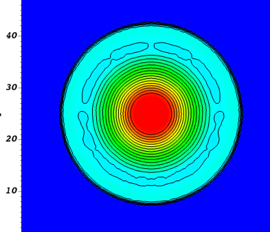
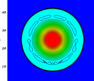
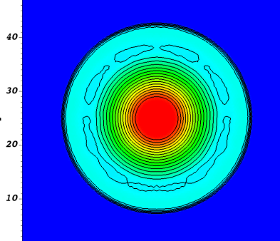
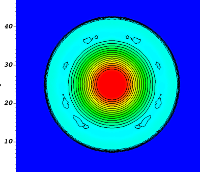
We run simulations using both the PAMPA-$\bm{u}$ and PAMPA-$\bm{v}$ schemes on a triangular mesh with 23266 elements and 46933 DoFs. As time progresses from the initial state $t=0$, the water begins to drain, and the waves start to propagate radially and symmetrically. We plot the numerical solution of water depth at the final time $t=0.69$ in Figure 9. Both two studied schemes produce correct results, with the waves propagating uniformly and symmetrically.

(a) PAMPA-$\bm{u}$: $\hbox{\vbox{\hrule height=0.5pt\kern 1.37775pt\hbox{\kern-0.40002pt$h$\kern 0.0pt}}}_{E}$

(b) PAMPA-$\bm{u}$: $h_{\sigma}$

(c) PAMPA-$\bm{u}$: $\hbox{\vbox{\hrule height=0.5pt\kern 1.37775pt\hbox{\kern-0.40002pt$h$\kern 0.0pt}}}_{E}$

(d) PAMPA-$\bm{u}$: $h_{\sigma}$

Figure 9: Example 5: Cell averages and point values of water depth at $t=0.69$ computed by the PAMPA-$\bm{u}$ (top row) and PAMPA-$\bm{v}$ (bottom row) schemes.

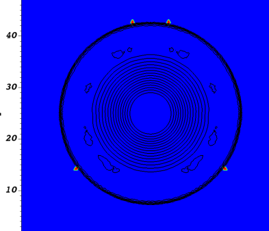
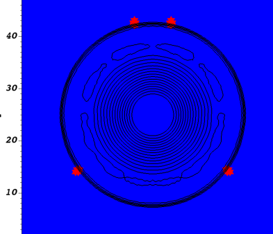
Finally, in Figure 10, we also plot the regions where the first-order scheme is activated at the final time for the PAMPA-$\bm{u}$ scheme. It is evident that the first-order scheme is only used in a few elements. For the PAMPA-$\bm{v}$ scheme, the first-order scheme is not activated at the final time $t=0.69$, so the corresponding figures are not shown.

(a) PAMPA-$\bm{u}$: flag on elements

(b) PAMPA-$\bm{u}$: flag on DoFs

Figure 10: Example 5: Flags at the positions where the first-order scheme is used for the PAMPA-$\bm{u}$ scheme.

Example 6—2-D Riemann Problem

In the final example, we test a 2-D Riemann problem with a complex wave structure. The bottom topography is flat $(i.e.,Z(x,y)=0)$ and the initial conditions are given by piecewise constant values in each of the four quadrants of a square domain $[0,100]\times[0,100]$:

$$(h(x,y,0),u(x,y,0),v(x,y,0))=\left\{\begin{aligned} &(10,0,0)&&\mbox{if}~{}50\leq x\leq 100~{}\mbox{and}~{}50\leq y\leq 100,\\ &(3,3,0)&&\mbox{if}~{}0\leq x\leq 50~{}\mbox{and}~{}50\leq y\leq 100,\\ &(0.2,3,3)&&\mbox{if}~{}0\leq x\leq 50~{}\mbox{and}~{}0\leq y\leq 50,\\ &(3,0,3)&&\mbox{if}~{}50\leq x\leq 100~{}\mbox{and}~{}0\leq y\leq 50.\end{aligned}\right.$$

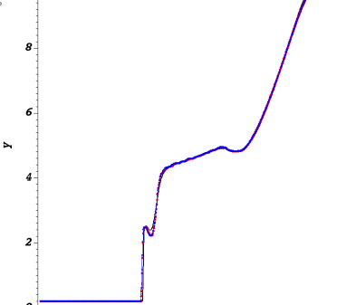
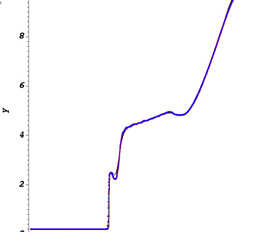
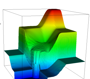
We compute the numerical solution using both the PAMPA-$\bm{u}$ and PAMPA-$\bm{v}$ schemes on a triangular mesh with 188968 elements and 379081 DoFs until a final time $t=3$. Results of both the cell averages and point values for the overview of water depth $h$ are shown in Figure 11, as well as a reference solution computed by the first-order PAMPA-$\bm{u}$ scheme on a much finer mesh with 578312 elements and 1158625 DoFs are presented. As one can observe, the results computed by either PAMPA-$\bm{u}$ or PAMPA-$\bm{v}$ schemes show a very good agreement with the reference solution. In the first quadrant, there are two interacting rarefaction waves moving in the $x$- and $y$-directions. In the second and fourth quadrants, there are two rarefaction waves moving in the $y$- and $x$-direction respectively, which interact with a transverse shock wave. In the third quadrant, the wave pattern becomes more complex. There are two shocks, moving perpendicularly with respect to each other, and from their interaction a jet stream pointing to the bottom-left corner of the domain. A cross-sectional representation of water depth $h$ is also presented in Figure 12. The results are generally considered satisfying and the methods are capable of reproducing correct solutions.

(a) PAMPA-$\bm{u}$: $\hbox{\vbox{\hrule height=0.5pt\kern 1.37775pt\hbox{\kern-0.40002pt$h$\kern 0.0pt}}}_{E}$

(b) PAMPA-$\bm{v}$: $\hbox{\vbox{\hrule height=0.5pt\kern 1.37775pt\hbox{\kern-0.40002pt$h$\kern 0.0pt}}}_{E}$

(c) Reference: $\hbox{\vbox{\hrule height=0.5pt\kern 1.37775pt\hbox{\kern-0.40002pt$h$\kern 0.0pt}}}_{E}$

(d) PAMPA-$\bm{u}$: $h_{\sigma}$

(e) PAMPA-$\bm{v}$: $h_{\sigma}$

(f) Reference: $h_{\sigma}$

Figure 11: Example 6: Overview of the water depth $h$ computed by the PAMPA-$\bm{u}$ (left column) and PAMPA-$\bm{v}$ (middle column) schemes as well as the reference solution (right column).

(a) $\hbox{\vbox{\hrule height=0.5pt\kern 1.37775pt\hbox{\kern-0.40002pt$h$\kern 0.0pt}}}_{E}$

(b) $h_{\sigma}$

Figure 12: Example 6: Cross-sectional representation of water depth in the diagonal direction. Comparison among the PAMPA-$\bm{u}$ (red), PAMPA-$\bm{v}$ (blue), and reference solution (black)

5 Conclusion

In this paper, we have presented new well-balanced PAMPA methods on unstructured triangular meshes for solving the two-dimensional Saint-Venant system of shallow water equations. In the proposed methods, the solution is a globally continuous representation of cell average within each triangular element, and point values located on the boundaries of these elements. The conservative property is recovered by evolving the cell averages in a conservative form, while there is greater flexibility in handling the evolution of the point values, which is governed by a non-conservative formulation of the same PDEs. Both conservative and primitive variables are considered when updating the point values. We have shown that both two studied schemes based on the conservative or primitive variables are well-balanced. We have also demonstrated that the proposed schemes are positivity-preserving by using the MOOD paradigm and the positivity-preserving first-order schemes. Several numerical examples with smooth and discontinuous problems have been tested to illustrate the performance of these methods. The results of both two studied PAMPA schemes are consistent and their behaviour is as expected. Moreover, the adoption of a non-conservative formulation and the use of primitive variables do not trigger any issues.

In future work, we plan to extend the proposed PAMPA method to include higher-order schemes and applications in more realistic and complex hyperbolic models, such as the thermal rotating shallow water equations. In this model, there is an additional advection type equation governing the evolution of the buoyancy (temperature gradient) field. Accurately resolving sharp temperature and pressure fronts is desirable. The non-conservative formulation written in terms of primitive variables may become more attractive and advantageous in this context.

Appendix A Formula of $\mathbf{S}_{E}^{2}$ in (13)

In this appendix, we provide the formula of the integral $\bm{S}_{E}^{2}$ in (13). After computing all the quantities $\int_{E}\varphi_{i}\nabla\varphi_{j}\,{\rm d}\bm{x}$, we obtain

$$\bm{S}_{E}^{2} =-g\Bigg{\{}Z_{\sigma_{1}}\bm{n}_{1}\Big{(}c_{1}\big{(}2w_{\sigma_{1}}-w_{\sigma_{2}}-w_{\sigma_{3}}\big{)}+c_{2}\big{(}w_{\sigma_{4}}+w_{\sigma_{6}}-2w_{\sigma_{5}}\big{)}\Big{)}$$

$$+Z_{\sigma_{2}}\bm{n}_{2}\Big{(}c_{1}\big{(}2w_{\sigma_{2}}-w_{\sigma_{1}}-w_{\sigma_{3}}\big{)}+c_{2}\big{(}w_{\sigma_{4}}+w_{\sigma_{5}}-2w_{\sigma_{6}}\big{)}\Big{)}$$

$$+Z_{\sigma_{3}}\bm{n}_{3}\Big{(}c_{1}\big{(}2w_{\sigma_{3}}-w_{\sigma_{1}}-w_{\sigma_{2}}\big{)}+c_{2}\big{(}w_{\sigma_{5}}+w_{\sigma_{6}}-2w_{\sigma_{4}}\big{)}\Big{)}$$

$$+Z_{\sigma_{4}}\bm{n}_{1}\Big{(}c_{4}\big{(}2w_{\sigma_{1}}+6w_{\sigma_{2}}-3w_{\sigma_{3}}-5\hbox{\vbox{\hrule height=0.5pt\kern 1.72218pt\hbox{\kern-0.50003pt$w$\kern 0.0pt}}}_{E}\big{)}+c_{5}\big{(}44w_{\sigma_{4}}+2w_{\sigma_{6}}-26w_{\sigma_{5}}-20\hbox{\vbox{\hrule height=0.5pt\kern 1.72218pt\hbox{\kern-0.50003pt$w$\kern 0.0pt}}}_{E}\big{)}\Big{)}$$

$$+Z_{\sigma_{4}}\bm{n}_{2}\Big{(}c_{4}\big{(}6w_{\sigma_{1}}+2w_{\sigma_{2}}-3w_{\sigma_{3}}-5\hbox{\vbox{\hrule height=0.5pt\kern 1.72218pt\hbox{\kern-0.50003pt$w$\kern 0.0pt}}}_{E}\big{)}+c_{5}\big{(}44w_{\sigma_{4}}+2w_{\sigma_{5}}-26w_{\sigma_{6}}-20\hbox{\vbox{\hrule height=0.5pt\kern 1.72218pt\hbox{\kern-0.50003pt$w$\kern 0.0pt}}}_{E}\big{)}\Big{)}$$

$$+Z_{\sigma_{4}}\bm{n}_{3}\Big{(}c_{6}\big{(}7w_{\sigma_{3}}-16w_{\sigma_{4}}+12w_{\sigma_{5}}+12w_{\sigma_{6}}-15\hbox{\vbox{\hrule height=0.5pt\kern 1.72218pt\hbox{\kern-0.50003pt$w$\kern 0.0pt}}}_{E}\big{)}\Big{)}$$

$$+Z_{\sigma_{5}}\bm{n}_{1}\Big{(}c_{6}\big{(}7w_{\sigma_{1}}+12w_{\sigma_{4}}-16w_{\sigma_{5}}+12w_{\sigma_{6}}-15\hbox{\vbox{\hrule height=0.5pt\kern 1.72218pt\hbox{\kern-0.50003pt$w$\kern 0.0pt}}}_{E}\big{)}\Big{)}$$

$$+Z_{\sigma_{5}}\bm{n}_{2}\Big{(}c_{4}\big{(}2w_{\sigma_{2}}+6w_{\sigma_{3}}-3w_{\sigma_{1}}-5\hbox{\vbox{\hrule height=0.5pt\kern 1.72218pt\hbox{\kern-0.50003pt$w$\kern 0.0pt}}}_{E}\big{)}+c_{5}\big{(}2w_{\sigma_{4}}+44w_{\sigma_{5}}-26w_{\sigma_{6}}-20\hbox{\vbox{\hrule height=0.5pt\kern 1.72218pt\hbox{\kern-0.50003pt$w$\kern 0.0pt}}}_{E}\big{)}\Big{)}$$

$$+Z_{\sigma_{5}}\bm{n}_{3}\Big{(}c_{4}\big{(}6w_{\sigma_{2}}+2w_{\sigma_{3}}-3w_{\sigma_{1}}-5\hbox{\vbox{\hrule height=0.5pt\kern 1.72218pt\hbox{\kern-0.50003pt$w$\kern 0.0pt}}}_{E}\big{)}+c_{5}\big{(}44w_{\sigma_{5}}+2w_{\sigma_{6}}-26w_{\sigma_{4}}-20\hbox{\vbox{\hrule height=0.5pt\kern 1.72218pt\hbox{\kern-0.50003pt$w$\kern 0.0pt}}}_{E}\big{)}\Big{)}$$

$$+Z_{\sigma_{6}}\bm{n}_{1}\Big{(}c_{4}\big{(}2w_{\sigma_{1}}-3w_{\sigma_{2}}+6w_{\sigma_{3}}-5\hbox{\vbox{\hrule height=0.5pt\kern 1.72218pt\hbox{\kern-0.50003pt$w$\kern 0.0pt}}}_{E}\big{)}+c_{5}\big{(}2w_{\sigma_{4}}-26w_{\sigma_{5}}+44w_{\sigma_{6}}-20\hbox{\vbox{\hrule height=0.5pt\kern 1.72218pt\hbox{\kern-0.50003pt$w$\kern 0.0pt}}}_{E}\big{)}\Big{)}$$

$$+Z_{\sigma_{6}}\bm{n}_{2}\Big{(}c_{6}\big{(}7w_{\sigma_{2}}+12w_{\sigma_{4}}+12w_{\sigma_{5}}-16w_{\sigma_{6}}-15\hbox{\vbox{\hrule height=0.5pt\kern 1.72218pt\hbox{\kern-0.50003pt$w$\kern 0.0pt}}}_{E}\big{)}\Big{)}$$

$$+Z_{\sigma_{6}}\bm{n}_{3}\Big{(}c_{4}\big{(}6w_{\sigma_{1}}-3w_{\sigma_{2}}+2w_{\sigma_{3}}-5\hbox{\vbox{\hrule height=0.5pt\kern 1.72218pt\hbox{\kern-0.50003pt$w$\kern 0.0pt}}}_{E}\big{)}+c_{5}\big{(}2w_{\sigma_{5}}+44w_{\sigma_{6}}-26w_{\sigma_{4}}-20\hbox{\vbox{\hrule height=0.5pt\kern 1.72218pt\hbox{\kern-0.50003pt$w$\kern 0.0pt}}}_{E}\big{)}\Big{)}$$

$$+\hbox{\vbox{\hrule height=0.5pt\kern 1.72218pt\hbox{\kern-0.50003pt$w$\kern 0.0pt}}}_{E}\Big{(}c_{3}\big{(}Z_{\sigma_{1}}\bm{n}_{1}+Z_{\sigma_{2}}\bm{n}_{2}+Z_{\sigma_{3}}\bm{n}_{3}\big{)}-\frac{2}{3}\big{(}Z_{\sigma_{5}}\bm{n}_{1}+Z_{\sigma_{6}}\bm{n}_{2}+Z_{\sigma_{4}}\bm{n}_{3}\big{)}\Big{)}$$

$$+\hbox{\vbox{\hrule height=0.5pt\kern 1.72218pt\hbox{\kern-0.50003pt$Z$\kern 0.0pt}}}_{E}\Big{(}\frac{2}{3}\big{(}(w_{\sigma_{5}}-w_{\sigma_{4}})\bm{n}_{1}+(w_{\sigma_{6}}-w_{\sigma_{4}})\bm{n}_{2}\big{)}$$

$$-c_{3}\big{(}(w_{\sigma_{1}}-w_{\sigma_{3}})\bm{n}_{1}+(w_{\sigma_{2}}-w_{\sigma_{3}})\bm{n}_{2}\big{)}\Big{)}\Bigg{\}},$$

where $\{\bm{n}_{i}\}_{i=1}^{3}$ are the inward normals defined in Section 2.1, and the coefficients $\{c_{j}\}_{j=1}^{6}$ are given by

$$c_{1}=\frac{1}{30},~{}~{}c_{2}=\frac{2}{45},~{}~{}c_{3}=\frac{1}{6},~{}~{}c_{4}=\frac{1}{90},~{}~{}c_{5}=\frac{1}{315},~{}~{}c_{6}=\frac{1}{126}.$$

References

• [1] R. Abgrall, Essentially non oscillatory residual distribution schemes for hyperbolic problems, J. Comput. Phys, 214 (2006), pp. 773–808.
• [2] R. Abgrall, A combination of Residual Distribution and the Active Flux formulations or a new class of schemes that can combine several writings of the same hyperbolic problem: application to the 1D Euler equation, Commun. Appl. Math. Comput., 5 (2023), pp. 370–402.
• [3] R. Abgrall and W. Barsukow, Extensions of Active Flux to arbitrary order of accuracy, ESAIM: Mathematical Modelling and Numerical Analysis, 57 (2023), pp. 991–1027.
• [4] R. Abgrall and W. Barsukow, A hybrid finite element–finite volume method for conservation laws, Appl. Math. Comput., 447 (2023), p. 127846.
• [5] R. Abgrall, J. Lin, and Y. Liu, Active flux for triangular meshes for compressible flows problems, (2024). arXiv:2312.11271.
• [6] R. Abgrall and Y. Liu, A new approach for designing well-balanced schemes for the shallow water equations: a combination of conservative and primitive formulations, (2024). https://doi.org/10.48550/arXiv.2304.07809.
• [7] E. Audusse, F. Bouchut, M.-O. Bristeau, R. Klein, and B. Perthame, A fast and stable well-balanced scheme with hydrostatic reconstruction for shallow water flows, SIAM J. Sci. Comput., 25 (2004), pp. 2050–2065.
• [8] W. Barsukow, The active flux scheme for nonlinear problems, J. Sci. Comput., 86 (2021), p. 34. Paper No. 3.
• [9] A. Beljadid, A. Mohammadian, and A. Kurganov, Well-balanced positivity preserving cell-vertex central-upwind scheme for shallow water flows, Computers & Fluids, 136 (2016), pp. 193–206.
• [10] W. Boscheri, M. Tavelli, and C. Castro, An all Froude high order IMEX scheme for the shallow water equations on unstructured Voronoi meshes, Appl. Numer. Math., 185 (2023), pp. 311–335.
• [11] S. Bryson, Y. Epshteyn, A. Kurganov, and G. Petrova, Well-balanced positivity preserving central-upwind scheme on triangular grids for the Saint-Venant system, M2AN Math. Model. Numer. Anal., 45 (2011), pp. 423–446.
• [12] S. Bryson and D. Levy, Balanced central schemes for the shallow water equations on unstructed grids, SIAM J. Sci. Comput., 27 (2005), pp. 532–552.
• [13] M. Ciallella, L. Micalizzi, P. Öffner, and D. Torlo, An arbitrary high order and positivity preserving method for the shallow water equations, Comput. Fluids, 247 (2022), p. 105630.
• [14] S. Clain, S. Diot, and R. Loubère, A high-order finite volume method for systems of conservation laws—multi-dimensional optimal order detection (MOOD), J. Comput. Phys., 230 (2011), pp. 4028–4050.
• [15] A. J. C. de Saint-Venant, Thèorie du mouvement non-permanent des eaux, avec application aux crues des rivière at à l’introduction des marèes dans leur lit., C.R. Acad. Sci. Paris, 73 (1871), pp. 147–154, 237–240.
• [16] H. Deconinck and M. Ricchiuto, Encyclopedia of Computational Mechanics, John Wiley & sons, 2007, ch. Residual distribution schemes: foundation and analysis. DOI: 10.1002/0470091355.ecm054.
• [17] A. Del Grosso, M. J. Castro, A. Chan, G. Gallice, R. Loubère, and P.-H. Maire, A well-balanced, positive, entropy-stable, and multi-dimensional-aware finite volume scheme for 2D shallow-water equations with unstructured grids, J. Comput. Phys., 503 (2024), p. 112829.
• [18] T. A. Eyman, Active flux, (2013). PhD thesis, University of Michigan.
• [19] T. A. Eyman and P. L. Roe, Active flux, in 49th AIAA Aerospace Science Meeting, 2011.
• [20] T. A. Eyman and P. L. Roe, Active flux for systems, in 20th AIAA Computational Fluid Dynamics Conference, 2011.
• [21] U. S. Fjordholm, S. Mishra, and E. Tadmor, Well-balanced and energy stable schemes for the shallow water equations with discontinuous topography, J. Comput. Phys., 230 (2011), pp. 5587–5609.
• [22] J. Gallardo, C. Parés, and M. Castro, On a well-balanced high-order finite volume scheme for shallow water equations with topography and dry areas, J. Comput. Phys., 227 (2007), pp. 574–601.
• [23] C. Geuzaine and J.-F. Remacle, Gmsh: a 3-D finite element mesh generator with built-in pre- and post-processing facilities, Int. J. Numer. Methods Eng., 79 (2009), pp. 1309–1331, https://doi.org/10.1002/nme.2579.
• [24] C. Helzel, D. Kerkmann, and L. Scandurra, A new ADER method inspired by the active flux method, J. Sci. Comput., 80 (2019), pp. 35–61.
• [25] A. Kurganov and D. Levy, Central-upwind schemes for the Saint-Venant system, M2AN Math. Model. Numer. Anal., 36 (2002), pp. 397–425.
• [26] A. Kurganov, Y. Liu, and V. Zeitlin, Interaction of tropical cyclone-like vortices with sea-surface temperature anomalies and topography in a simple shallow-water atmospheric model, Phys. Fluids, 33 (2021), p. 106606.
• [27] A. Kurganov, Y. Liu, and V. Zeitlin, Thermal versus isothermal rotating shallow water equations: comparison of dynamical processes by simulations with a novel well-balanced central-upwind scheme, Geophys. Astrophys. Fluid Dyn., 115 (2021), pp. 125–154.
• [28] A. Kurganov and G. Petrova, A second-order well-balanced positivity preserving central-upwind scheme for the Saint-Venant system, Commun. Math. Sci., 5 (2007), pp. 133–160.
• [29] A. Kurganov, Z. Qu, and T. Wu, Well-balanced positivity preserving adaptive moving mesh central-upwind schemes for the Saint-Venant system, ESAIM: Mathematical Modelling and Numerical Analysis, 56 (2022), pp. 1327–1360.
• [30] R. J. LeVeque, Balancing source terms and flux gradients in high-resolution Godunov methods: the quasi-steady wave-propagation algorithm, J. Comput. Phys., 146 (1998), pp. 346–365.
• [31] Y. Liu and W. Barsukow, An arbitrarily high-order fully well-balanced hybrid finite element-finite volume method for a one-dimensional blood flow model, (2024). arXiv:2404.18124.
• [32] Y. Liu, J. Lu, Q. Tao, and Y. Xia, An oscillation-free Discontinuous Galerkin method for shallow water equations, J. Sci. Comput., 92 (2022). Paper No. 109, 24 pp.
• [33] M. Lukáčová-Medvid’ová, S. Noelle, and M. Kraft, Well-balanced finite volume evolution Galerkin methods for the shallow water equations, J. Comput. Phys., 221 (2007), pp. 122–147.
• [34] Y. Mantri, P. Öffner, and M. Ricchiuto, Fully well-balanced entropy controlled discontinuous Galerkin spectral element method for shallow water flows: global flux quadrature and cell entropy correction, J. Comput. Phys., 498 (2024), p. 112673.
• [35] S. Noelle, N. Pankratz, G. Puppo, and J. R. Natvig, Well-balanced finite volume schemesof arbitrary order of accuracy for shallow water flows, J. Comput. Phys., 213 (2006), pp. 474–499.
• [36] S. Noelle, Y. Xing, and C.-W. Shu, High-order well-balanced finite volume WENO schemes for shallow water equation with moving water, J. Comput. Phys., 226 (2007), pp. 29–58.
• [37] B. Ren, Z. Gao, Y. Gu, S. Xie, and X. Zhang, A positivity-preserving and well-balanced high order compact finite difference scheme for shallow water equations, Commun. Comput. Phys., 35 (2024), pp. 524–552.
• [38] F. Vilar, A posterior correction of high-order discontinuous Galerkin scheme through subcell finite volume formulation and flux reconstruction, J. Comput. Phys., 387 (2019), pp. 245–279.
• [39] Y. Xing and C.-W. Shu, High-order finite volume WENO schemes for the shallow water equations with dry states, Adv. Water Resour., 34 (2011), pp. 1026–1038.
• [40] R. Yan, W. Tong, and G. Chen, A well-balanced positivity-preserving multidimensional central scheme for shallow water equations, Appl. Numer. Math., 197 (2024), pp. 97–118.
• [41] J. Zhang, Y. Xia, and Y. Xu, Structure-preserving finite volume arbitrary Lagrangian-Eulerian WENO schemes for the shallow water equations, J. Comput. Phys., 473 (2023), p. 111758.
• [42] Z. Zhao and M. Zhang, Well-balanced fifth-order finite difference Hermite WENO scheme for the shallow water equations, J. Comput. Phys., 475 (2023), p. 111860.