Is Tokenization Needed for Masked Particle Modelling?

Abstract

In this work, we significantly enhance masked particle modeling (MPM), a self-supervised learning scheme for constructing highly expressive representations of unordered sets relevant to developing foundation models for high-energy physics. In MPM, a model is trained to recover the missing elements of a set, a learning objective that requires no labels and can be applied directly to experimental data. We achieve significant performance improvements over previous work on MPM by addressing inefficiencies in the implementation and incorporating a more powerful decoder. We compare several pre-training tasks and introduce new reconstruction methods that utilize conditional generative models without data tokenization or discretization. We show that these new methods outperform the tokenized learning objective from the original MPM on a new test bed for foundation models for jets, which includes using a wide variety of downstream tasks relevant to jet physics, such as classification, secondary vertex finding, and track identification.

1 Introduction

The field of high-energy physics (HEP) has increasingly integrated machine learning (ML) methods to tackle diverse challenges, including event reconstruction, anomaly detection, and data generation. These developments have largely mirrored the trends of the wider ML community. Model sizes across all fields have grown exponentially, and transformer-based neural networks have become the dominant architecture for many tasks. However, despite some initial studies [1, 2, 3, 4, 5, 6, 7, 8], HEP has yet to truly adopt foundation models (FMs) [9], large pre-trained models that can be fine-tuned on many downstream tasks, which are prevalent in the fields of natural language processing (NLP) [10, 11, 12, 13, 14] and computer vision (CV) [15, 16, 17, 18, 19, 20].

An FM is exposed to a large corpus of domain-related data with the goal of learning expressive representations of the subject matter. This is referred to as pre-training, and it is usually self-supervised; the model is given input samples but no associated truth labels. Once pre-trained, FMs are fine-tuned on specific tasks in a supervised manner. In NLP, typical pre-training tasks consist of predicting the next token in the input sequence (GPT [11]) or predicting randomly masked tokens (BERT  [10]), and typical downstream tasks include sentiment analysis and machine translation. In downstream tasks, the FM is frequently called the backbone because, although additional learnable layers may be necessary, it holds the bulk of the parameters.

The self-supervised learning (SSL) paradigm is particularly advantageous for HEP because experimental data is unlabelled. For many tasks in HEP, supervised training is only possible using simulated datasets, where the truth labels are derived from the simulator itself. Running high-quality physics simulations [21] is a time-consuming process. Furthermore, these simulations do not perfectly model real data, causing a domain shift between the synthetic samples the model was trained on and the real data to which it is then applied. Therefore, we are highly motivated to develop SSL techniques for producing FMs that can be trained directly on real data.

In this work, we iterate upon Golling et al. [1], which introduced a SSL strategy designed to run on unordered sets of objects and targeted applications to particles. The particles are reconstructed objects derived from detector signals captured during a high-energy collision, such as those produced in the Large Hadron Collider (LHC). The attributes associated with each particle include its kinematics (energy and momentum), particle type, charge, and additional features pertaining to its reconstruction. In MPM, we are given a set of attributed particles, a random subset is masked, and the model is tasked to reconstruct it. MPM is analogous to masked language modeling, as in BERT [10], or masked image modeling, as in BEiT [20]. But unlike images and text, the particle sets have no natural ordering.

It is possible to frame masked modeling in the context of denoising autoencoders (DAE) [22]. In a DAE, a lossy augmentation is first applied to the inputs, which are then projected via an encoder to a latent space. A decoder is used to map back to the original uncorrupted signal. Once the DAE is trained, only the encoder is saved for further applications, while the decoder is typically discarded. Masking or removing elements from the input sample is a simple, fast, and effective corruption method that underpins many notable models in NLP and CV [10, 11, 13, 19, 20, 23, 24, 25, 26, 27]. Masked pre-training requires little prior knowledge of the data and can be applied to a wide variety of fields. This is the approach taken by MPM.

Many stable particles are produced in any given collision event, which are subsequently captured by the detector. However, in this work, we focus on particle jets. Jets are collimated sprays of particles produced by the hadronization of quarks and gluons. Multiple jets can be created in an event, and we treat each as a complete set. The structure and composition of these sets depend highly on the type of particle that produced it. As an experimental signature of particles with the colored charge, they are key ingredients in studying quantum chromodynamics, the Standard Model, and searches for new physics. MPM is a method for training an FM, which can either be fine-tuned or used simply as a fixed encoder for various supervised downstream tasks related to the study of jets.

As most of the particles’ features are continuous, we could not naively apply the same successful training strategy as language models like BERT or GPT. These models predict the full probability distribution function (PDF) for the masked or next token, an embedding that contains rich semantic information [19]. Naive regression methods on continuous variables do not produce the same informative output. Inspired by the approach used for images in BEiT, the original MPM model, hereto referred to as MPMv1, was trained to recover tokenized representations of each particle derived from a separately trained Vector-Quantized Variational Autoencoder (VQVAE) [28]. The VQVAE maps the input jet to a set of discreet codebook elements and back again. Borrowing the language used in BEiT, the VQVAE-encoder is our particle tokenizer. This changes the MPM reconstruction task from regression to classification, as the FM is tasked to predict the codebook ID of the tokenized particle

Golling et al. [1] found that using the VQVAE-derived targets during pre-training leads to a more performant FM than direct regression and argued that this was primarily due to two reasons: (1) The VQVAE latent space is semantically rich, containing high-level abstractions, giving the MPMv1 encoder a more informative target to learn from (this is also the justification used in BEiT). (2) By changing from a regression to a classification task, the backbone is taught the full conditional posterior distribution rather than just seeking the mean, which is much more expressive. However, producing the VQVAE requires an additional training step in the pipeline. VQVAEs are notoriously unstable and hard to train. Furthermore, the aforementioned quantization leads to a loss of information.

In this paper, we make the following contributions. (1) We propose an improved MPM training paradigm, named MPMv2, by enhancing model architecture and addressing existing inefficiencies. We also expand the particle attributes to provide a more detailed representation. (2) We provide a detailed study of alternative reconstruction tasks for MPMv2 pre-training, ones that replace the costly VQVAE-derived targets. (3) We provide a new test bed for pre-trained models that include a wider set of downstream tasks commonly encountered in jet physics.

2 Related Work

In addition to MPM, there have been several other works in developing foundation models for physics. One of the first notable attempts is JetCLR [8], which uses the SimCLR [29] framework to pre-train a fixed encoder. JetCLR uses approximate but physically inspired augmentations, such as rotations of the constituents about the jet axis and the smearing of soft constituents to estimate soft gluon radiation. The SimCLR framework was used again for Re-Simulation-based Self-Supervised Learning (R3SL) [2]. This framework explicitly requires simulated data as each positive pair is the same underlying event, duplicated at some point in the simulation pipeline, and then completed with different seeds or settings. OmniJet-$\alpha$ is another recent work that uses a similar approach to MPM but swaps the masked reconstruction pre-training for GPT style next token prediction. Similar to MPM, Kishimoto et al. [3] devised a pre-training strategy where only the particle type is masked and reconstructed. The kinematics and other continuous features are always available to the model. The work by Vigl et al. [4] proposes to describe various elements of the reconstruction pipeline as viable pre-training tasks. Finally, the Omnilearn [6] model is pre-trained jointly as a supervised classifier for jets and as a diffusion generative model.

3 Data

3.1 Datasets

A key aspect of MPM is that it does not require labels and can thus be applied directly to experimental data. However, because large open datasets of real jets are not available, we use MC simulations to refine the framework. Crucially, we still ignore the truth labels during pre-training, and the only conclusions we draw in this paper are between models trained on the same datasets. Access to the truth labels also gives us a means to evaluate the performance of the FMs.

We focus on two datasets, both of which utilize the Delphes [30] simulation package. The first is the publicly available JetClass dataset [31], which contains 120 million large radius jets equally distributed amongst 10 classes. Each class represents a different physical process and decay chain, such as $H\rightarrow 4q$ and $t\rightarrow b\ell\nu$. The second dataset we label BTag, which contains 3 million jets from three classes differentiated by the flavor of quark which initiated the jet, light, charm, or bottom.

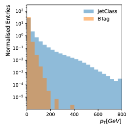
Events in both JetClass and BTag are generated using Pythia8 [32], but jets in JetClass arising from top, W, Z, or Higgs decays are additionally modeled with MadGraph5 [33]. Both datasets reconstruct their jets using calorimeter energy deposits with the anti-kt algorithm [34]; the radius parameter is set to $R=0.8$ for JetClass and $R=0.4$ for BTag. JetClass jets have significantly higher transverse momentum of 500-1000 GeV, whereas BTag only requires $p_{\text{T}}\geq 20$ GeV. Additionally, JetClass uses a Delphes configuration that matches the CMS experiment [35] while BTag is configured to match the ATLAS experiment [36]. The final significant difference is that JetClass contains both charged and neutral constituents, while BTag only contains charged particles. As such, JetClass jets have a higher cardinality, averaging around 50 constituents per jet, whereas BTag jets are capped at 15.

We only use JetClass to pre-train our models, but we fine-tune and evaluate using both datasets. The differences between these datasets represent the realistic variations in how particle physics jets are defined in different experimental settings. Targeted kinematic ranges, reconstruction parameters (like the anti-kt radius), and object selection vary significantly depending on the physics analyses and are finely tuned by experts. These differences offer a chance to view the backbone’s generalizability to new downstream tasks and a new out-of-distribution (OOD) dataset.

In Golling et al. [1], each massless constituent is represented using only its kinematics relative to the jet axis, $(p_{\text{T}},\Delta\eta,\Delta\phi)$. We expand this to include common reconstructed attributes used in experimental settings. For charged constituents, which leave tracks in the detector, we include the lifetime signed longitudinal and transverse impact parameters ($d_{0}$, $z_{0}$) as well as their reconstruction uncertainties ($\sigma(d_{0})$, $\sigma(z_{0})$) [37]. Neutral particles have no defined impact parameters, so these are zero-padded. These 7 variables form the continuous features of the particle, $x^{\text{c}}$. Also included is the particle identity (ID) $x^{\text{id}}$, a one-hot encoded vector that categorizes both the particle type and charge into 8 independent classes. To summarize, a jet is an unordered set of N particles, each represented by a vector of 8 features, 7 continuous and one categorical, $X=\{x_{i}=(x^{\text{c}}_{i},x^{\text{id}}_{i})\}_{i=1}^{N}$.

4 Method

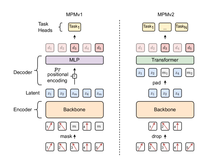
In MPMv1, $M$ particles out of the $N$ that constitute the jet are selected, and all of their features are replaced with a special masked token. The goal is then to recover those features, or at least tokenized representations of them.

Framing MPMv1 as a DAE, the input sample $\mathcal{X}=\{x_{i}\}_{i=1}^{N}$, its latent projection $\mathcal{Z}$, and the decoder output $\mathcal{D}$ are all sets, so all mappings between them must be permutation equivariant. Therefore, the encoder is not provided with positional encoding (PE). Given $\mathcal{X}$, we define the corrupted sample as the union of the surviving subset and a set of identical masked tokens $\mathcal{S}=\{x_{i}\}_{i=1}^{M}~{}\cup~{}\{m\}_{1}^{N-M}$. A transformer acts as the encoder, and a multi-layer perceptron (MLP) acts as the decoder, applied separately per set element. A consequence of having no PE is that the encoder’s outputs corresponding to masked inputs are duplicates. Golling et al. [1] is forced to inject PE based on $p_{\text{T}}$ in the latent space to break this degeneracy for reconstruction while keeping the encoder equivariant. Each element in $\mathcal{D}$ is then used in the tokenized reconstruction task, where it is compared to the corresponding element of the same jet passed through the encoder of a VQVAE.

We propose a number of alterations to this model for MPMv2. The repeated use of the same masked token in the encoder means that the transformer layers perform identical operations, wasting computation. We found that it was significantly more efficient to remove all masked tokens from the input set and reintroduce them only during decoding. This means that $\mathcal{Z}$ has a lower cardinality than both $\mathcal{X}$ and $\mathcal{D}$. This change reflects a departure of a model similar to BERT [10] to a model more akin to MAE [19]. As such, we also experimented with expanding the decoder to a full transformer and saw greatly improved results. The decoder is designed similarly to the encoder, albeit much smaller. It has one-quarter of the embedding dimension, fewer layers, and fewer attention heads. With the new decoder, full PE in the latent space provides too much information, trivializing the reconstruction task, which hurts the FM performance. We find it sufficient to provide PE between the masked elements, not the full jet. This is achieved by using a unique mask token depending on the $p_{\text{T}}$ order of the dropped constituents with respect to each other only. The loss function is then derived by comparing $\mathcal{X}$ and $\mathcal{D}$ in a variety of reconstruction tasks.

Figure 1: A comparison of the original MPM encoder-decoder setup (left) and the new model configuration (right). The new model includes multiple reconstruction tasks, swaps the MLP decoder for a transformer, and only encodes the reduced set.

4.1 Reconstruction Tasks

Where MPMv1 only utilized a VQVAE-derived reconstruction task, we now experiment by combining multiple tasks to recover the continuous and categorical features separately. Each task requires extra learnable layers (task head) and contributes a loss term, which is summed for the combined pre-training. We investigate 5 different reconstruction tasks for the continuous features $x^{\text{c}}$ and an extra task for the categorical features $x^{\text{id}}$.

Particle Identification

The first task is simply to recover the particle type $x^{\text{id}}$ of the dropped constituents. This is a standard classification problem, so we use a linear layer and the cross-entropy loss function for the task head.

VQVAE-Tokenized Classification

We include the method used in the original MPM work. A VQVAE is first trained to embed the jet, using only the continuous features, to a set of indices representing the elements in a learned codebook. We used a codebook size of $1024$ and a codebook vector dimension of 32 following Yu et al. [38]. We use a linear layer and the cross-entropy loss function for the task head.

Direct Regression

While Golling et al. [1] found direct regression to be insufficient for pre-training, we believe it is worth revisiting owing to the much more powerful decoder. We use a linear layer and find the best results by using the L1-loss to recover the particles’ continuous features.

K-Means Tokenized Classification

If the VQVAE does not provide a sufficiently semantically rich latent space, its benefit may be simply that it creates a classification task. Regression is mean-seeking, while the tokenized classification allows us to learn the full conditional posterior of the dropped features, albeit in a discretized form. To test this, we trial a more trivial token reconstruction task using K-Means centroids. We fit the K-Means using $x^{\text{c}}$ and the first 1 million jets in JetClass. Based on preliminary tests, we found that $K=16384$ is the optimal number of centroids. Fitting the K-Means using the torchpq library [39] took significantly less time than training the VQVAE. Like the other tasks, we used a single linear layer to map to this space and cross-entropy loss function.

Conditional Normalizing Flow

If the strength of the tokenized form of reconstruction over regression is in learning the full posterior distribution $p(x^{\text{c}}_{i}|d_{i})$, it is possible that we can reproduce this using a generative model. This also means we do not suffer from the information loss that comes with discretization. One choice of model is a conditional normalizing flow (CNF) [40], which we implement using the normflows library [41]. The CNF contains 6 rational-quadratic-spline coupling blocks and a Gaussian base distribution. Each block contains a two-layer MLP, which outputs the spline parameters for half the features of $x^{\text{c}}_{i}$ given the other half and the context information $d_{i}$. It is trained to maximize the log-likelihood of the transformation.

Conditional Flow-Matching

In recent years, diffusion-based generative models have emerged as the go-to methods for generating high-quality data. Various frameworks exist that try to generalize and describe this family of models [42, 43, 44, 45]. We follow the conditional flow-matching (CFM) framework from Lipman et al. [44]. Here, a model learns the probability vector field between the data distribution and a noise distribution parameterized by time $t\in[0,1]$. We consider a time-dependent pdf $p(x,t)$ which connects samples drawn from a data distribution $x_{0}\sim p_{0}(x)=p(x,0)$ to samples drawn from a noise distribution $\epsilon\sim p_{1}(x)=p(x,1)$. Instead of constructing $p(x,t)$ directly, we could equivalently construct the vector field $u(x,t)$, which relates to the pdf via the continuity equation,

$$\frac{\partial}{\partial t}p(x,t)=-\nabla\cdot(p(x,t)u(x,t)).$$ (1)

We use a neural network to approximate the velocity vector $u_{\theta}\approx u$, where $\theta$ represents the trainable weights. Directly learning the velocity via the flow-matching objective

$$L_{FM}=\mathop{\mathbb{E}}_{t,x_{t}\sim p_{t}(x)}||u_{\theta}(x_{t},t)-u(x_{t},t)||^{2},$$ (2)

is intractable. Instead, we can learn the conditional probability paths via the CFM loss,

$$L_{CFM}=\mathop{\mathbb{E}}_{t,\epsilon\sim p_{1},x_{t}\sim p_{t}(x|\epsilon)}||u_{\theta}(x_{t},t)-u(x_{t},t|\epsilon)||^{2},$$ (3)

These two objectives are equivalent for network training $\nabla_{\theta}L_{FM}=\nabla_{\theta}L_{CFM}$ (under all expectations). Moreover, $u(x_{t},t|\epsilon)$ and $p_{t}(x|\epsilon)$ do have specific tractable forms. One such form is $u(x_{t},t|\epsilon)=\frac{\epsilon-x_{t}}{1-t}$ which leads to Gaussian probability paths.

In practice, we derive the training objective given the continuous features of a particle $x^{\text{c}}_{i}$ and the corresponding decoder output $d_{i}$. We first sample a diffusion time $t$ using the logit-norm distribution from Sauer et al. [46] and sample from the noise distribution $\epsilon\sim\mathcal{N}(0,I)$. We mix the noise and the original features using a basic linear interpolant to get ${x^{\text{c}}_{i}}_{t}=(1-t)x^{\text{c}}_{i}+t\epsilon$. The target for the model is the velocity vector $u_{i}=x^{\text{c}}_{i}-\epsilon$, which we approximate using a three-layer MLP with a hidden dimension of 256, which takes as inputs ${x^{\text{c}}_{i}}_{t}$, $d_{i}$, and a cosine-embedded form of $t$ following Leigh et al. [47]. The resulting loss function is written as

$$L_{CFM}=||u_{\theta}({x^{\text{c}}_{i}}_{t},d_{i},t)-(x^{\text{c}}_{i}-\epsilon)||^{2}.$$ (4)

4.2 Set-to-set Flow-Matching

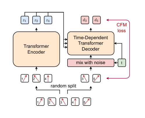
We also investigate a set-to-set flow-matching model (SSFM). The SSFM uses a time-dependent transformer decoder to generate the entire set of constituents given the set of latent nodes. This setup is similar to the diffusion-masked autoencoder from CV [48]. As with MPM, the input set $\mathcal{X}$ is split into a reduced set $\mathcal{S}$ and its complement $\mathcal{T}$. The reduced set is passed through the encoder to get the latent set $\mathcal{Z}$, which is used in the decoder’s cross-attention layers. The decoder is trained as a set-CFM model to generate the remaining set $\mathcal{T}$. A diagram of this model is shown in Figure 2. Since the loss is based purely on denoising the $\mathcal{T}$, degeneracy is not an issue, and no positional encoding or mask tokens are required. By varying the masking rate $D_{f}=\frac{M}{N}$, we can control the amount of jet generated by the diffusion model. The decoder is a standard diffusion generator when the $D_{f}=0$. Thus, our pre-training setup produces a backbone for embedding and a purely generative model for the jets akin to Omnilearn and Omnijet-$alpha$. During training, we sample $D_{f}\sim\mathcal{U}(0,0.8)$ to balance these two objectives.

Figure 2: A schematic overview of the SSFM model.

5 Results

5.1 Ablation Studies

To evaluate our proposed alterations to MPMv1, we use the new backbone as a fixed encoder to classify the JetClass dataset. After pre-training for 200k steps, we freeze the encoder and append a classifier-head, made from 2 class-attention layers [49] followed by a linear layer. We then train the head as a classifier with cross-entropy loss for another 200k steps. We elected to use only the regression, K-Means, and particle ID tasks for the ablation study as they were the quickest to prototype. The full results using all reconstruction tasks are shown in Section 5.2.

We present the results of the ablation study in Table 1. Initially, we recreated the training setup from Golling et al. [1], with the same masking rate of $D_{f}=0.3$. Next, we test the setup with more up-to-date transformer layers, described in Appendix A. Then, we add the impact parameters to the features of the particles, followed by including the particle ID inputs and ID reconstruction task. Each of these steps improves the classification accuracy of both models. The largest improvement comes from changing the decoder to a transformer. This step significantly increased the accuracy of the regression task, bringing the gap between the two methods from 10.5% to 2.2%. To verify the impact of the decoder change, we reran the regression task without the impact parameters or particle ID task. We found that it achieved an accuracy of 65.0%, an increase of 9.5%. Another major benefit of switching to the MAE setup was a 40% reduction in GPU memory due to the reduced point cloud size being passed to the encoder. Finally, we also experimented with adding registers into the encoder [50], which prevents the transformer from overwriting elements in the set with global information. We added 8 registers to the training and found that the classifier’s performance increased with little computational cost. Additionally, we optimized the mask rate and the decoder depth for the final training sessions.

Table 1: The effects of the model redesign on the accuracy of a classifier head trained using the encoder outputs. All models except the final iteration were trained using 200k training steps, a mask rate of 30%, and a 2-layer decoder.

	regression		k-means
MPMv1 using $(p_{\text{T}},\eta,\phi)$ [1]	48.9		56.2
+ updated transformer layers	55.5	$\uparrow 6.6$	62.2	$\uparrow 6.0$
+ impact parameter features	62.2	$\uparrow 6.7$	70.2	$\uparrow 8.0$
+ constituent ID feature and ID reconstruction task	63.5	$\uparrow 1.3$	74.0	$\uparrow 3.8$
+ transformer as decoder (MAE)	79.2	$\uparrow 15.7$	81.4	$\uparrow 7.4$
+ registers	80.4	$\uparrow 1.2$	83.0	$\uparrow 1.6$
+ longer train (1M steps) + deeper decoder + 40% mask rate	83.3	$\uparrow 2.0$	84.0	$\uparrow 1.0$

5.2 Downstream Tasks

Here, we evaluate the performance of our backbones on a variety of downstream tasks typically encountered in jet physics. Each backbone is pre-trained using one of the continuous feature reconstruction tasks (which it is named after) together with the particle ID task. Pre-training is run for 1M steps after which specific downstream task layers are appended to the encoder, and the model is fine-tuned. Finetuning is run for 200k steps, allowing for early stopping using a validation set. We use a randomly initialized network as a baseline to highlight the performance provided by pre-training and repeat each experiment 5 times to estimate the run-to-run variance.

5.2.1 In-Distribution Classification

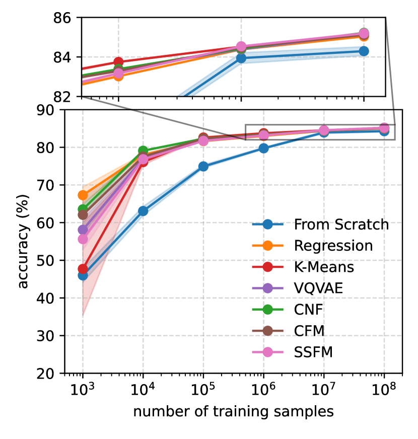
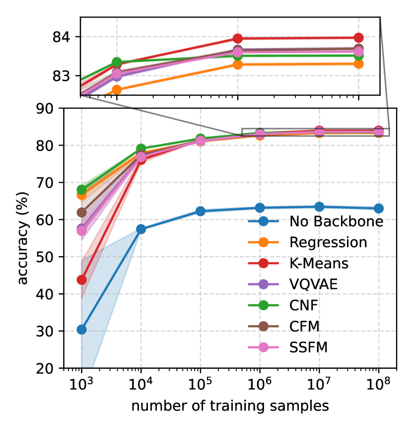
We perform classification on the JetClass dataset using the same classifier head described in Section 5.1. The backbone’s data efficiency is measured by varying the number of jets used to train the classifier from 1k to 100M, and these results are shown in Figure 3(a). At each training set size, the performance of all pre-trained backbones is superior to the randomly initialized network. However, this boost diminishes as the number of jets increases. At the maximum 100M jets, all backbones achieve an accuracy between 85.0% (regression) and 85.3% (K-Means), whereas the random initialization achieves 84.3%. Interestingly, the K-Means backbone performs best with more data, while the CNF and Regression backbones are more data-efficient. The Flow-backbone achieves the same performance with 10k jets as the randomly initialized network with 1M.

5.2.2 Weakly Supervised Classification

In many experimental settings, we are unable to produce perfectly labeled data, so we are interested in model performance in a setting where the labels are noisy or incomplete. The principle of classification without labels (CWoLa) [51] is that the ideal classifier between two mixed datasets with different signal and background proportions is the same as the ideal classifier between the two pure datasets. This is utilized in template-based anomaly detection [52, 53, 54, 55, 56, 57] and in muon isolation [58].

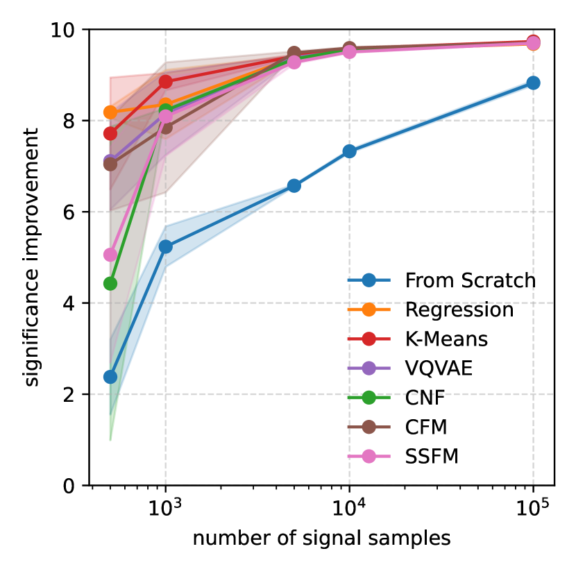
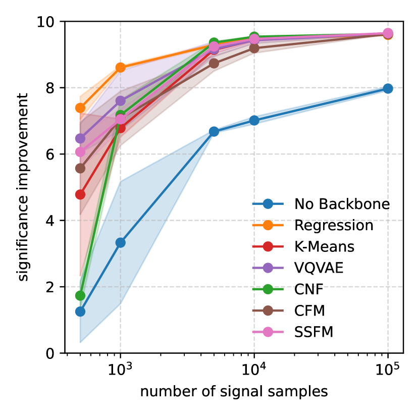
We emulate the CWoLa setting using two datasets of 500k QCD jets. Into one of the datasets, we inject top-initiated jets as a signal. We use the same classifier head as in the previous experiments. In Figure 3(b), we show the significance improvement (SIC) [59] from applying the classifiers on a test set containing pure samples of QCD background and top signal. The SIC is defined as the signal efficiency (true-positive rate) divided by the square root of the background efficiency (false-positive rate) at a 99% background rejection. The pre-trained backbones considerably outperform the benchmark, with the Regression backbone performing the best when only 500 top jets are present in the training set, resulting in a (SIC) of 8.18.

(a)

(b)

Figure 3: The in-distribution performance of the fine-tuned models on the JetClass dataset. (3(a)) shows the accuracy using standard supervised classification as a function of the dataset size. (3(b)) shows the significance-improvement of the models trained in a CWoLa setting as a function of the number of signal samples in the dataset.

5.2.3 Out-of-Distribution Classification

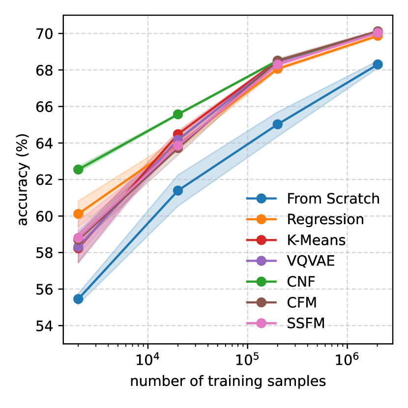
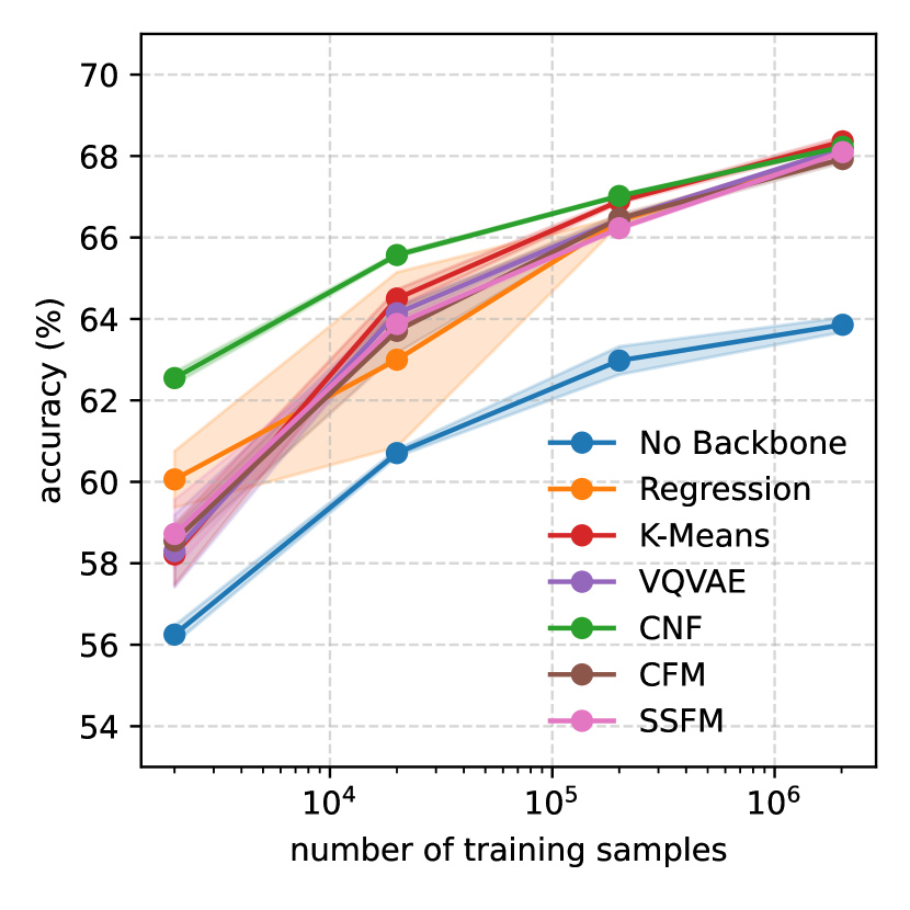
Here, we test the backbones’ performance in classifying the BTag dataset, which contains lower-energy, narrower jets with only a few charged particles. In Figure 4(a), we show the accuracy of the 3-class classifier as a function of the number of jets used for training. All pre-trained backbones outperform the benchmark initialization, indicating that the learned mappings are generalizable beyond JetClass. In this task, the CNF backbone performs the best, but all pre-trained backbones converge at around 70% accuracy with the maximum number of jets.

5.2.4 Secondary Vertex Finding

A track vertex refers to a common point where reconstructed particle tracks originate, indicating the location of an interaction or decay. Bottom and charm hadrons produced in the collision will survive long enough to travel several millimeters beyond the interaction point before decaying. This leads to multiple vertices existing within the same jet, and discovering them is a key intermediate step used in the identification of heavy-flavor jets  [60, 61], such as those initiated by bottom and charm hadrons. The decay of kaons also causes additional vertices. Secondary vertex finding is a task that partitions the jet’s tracks into groups that all originate from the same vertex. It is typically recast as an edge classification task, where given any two tracks, the pair is classified as either being part of the same vertex or not. This means that for a jet with N tracks, there are $N(N-1)/2$ unique pairs to test.

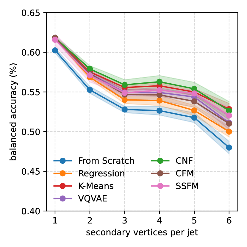
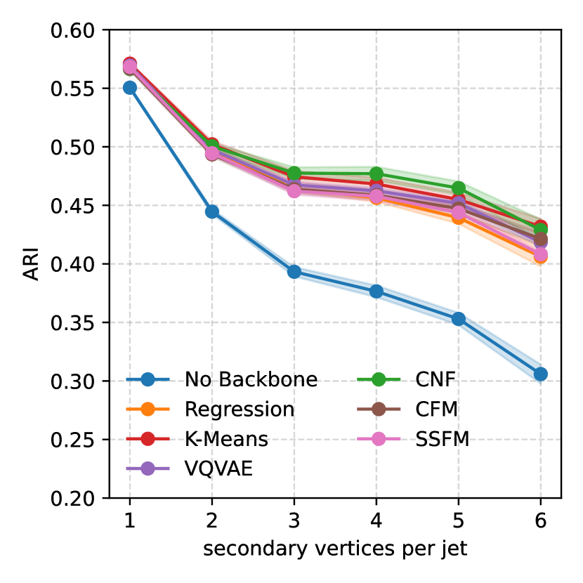
The additional layers for this task followed a twin-network approach [62]. Whereby the probability that two tracks $x_{i}$ and $x_{j}$ came from the same vertex was defined by $\sigma\left(G\left[|F\left(z_{i}\right)-F\left(z_{j}\right)|\right]\right)$, where $G,F$ are MLPs, $z_{i},z_{j}$ are the outputs of encoder, and $\sigma$ is the sigmoid function. Following Shlomi et al. [61], we use the adjusted Rand index (ARI) [63] as the performance metric. We plot the ARI as a function of the number of secondary vertices in Figure 4(b). Here, we find that the best-performing model is the backbone trained using the CNF task, though all backbones perform better than the benchmark.

5.2.5 Heavy Track Identification

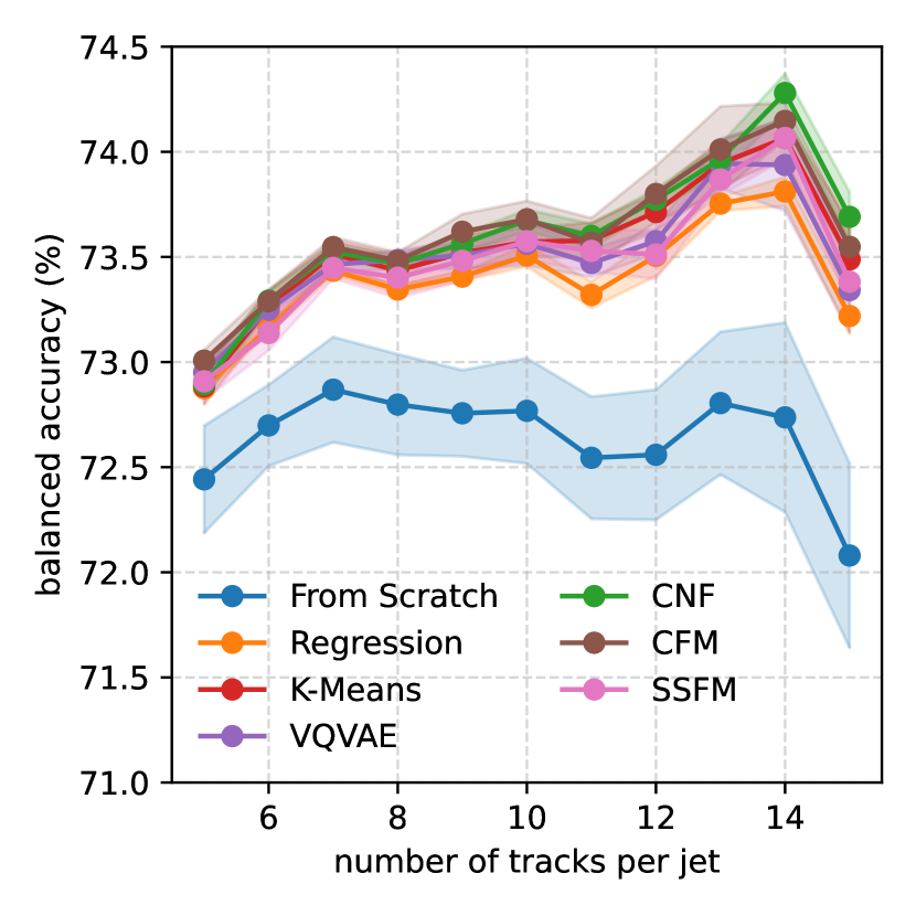
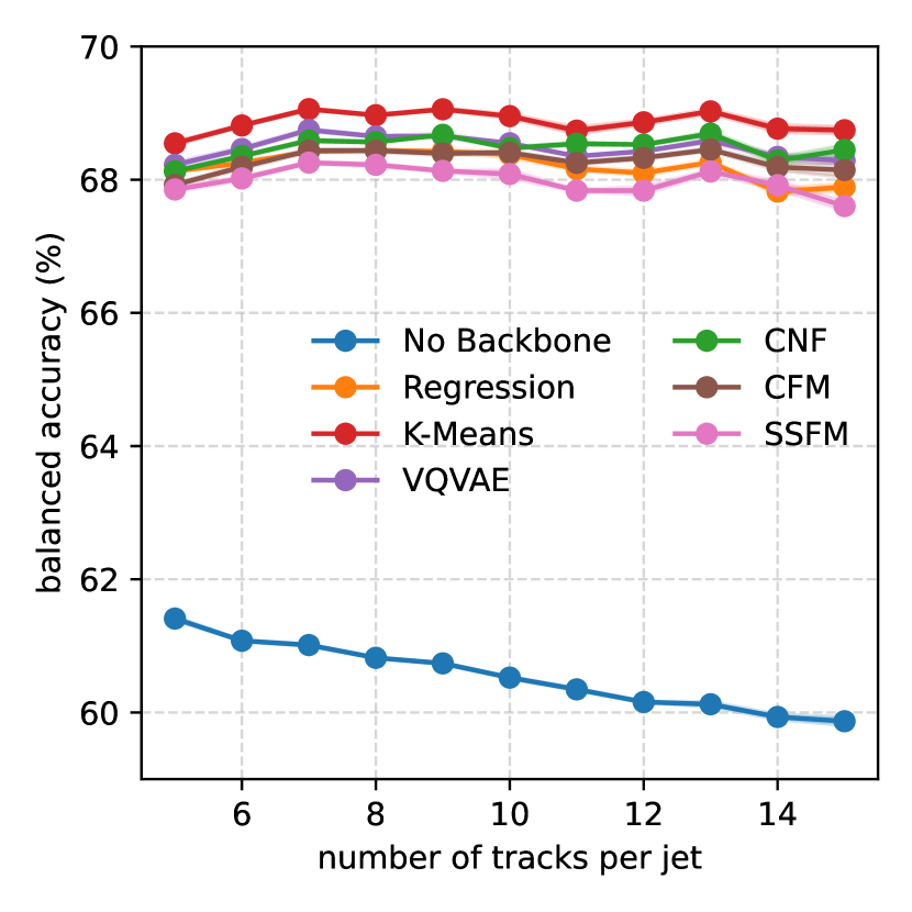
Where the vertex finding task grouped tracks that shared a vertex, we can also attempt to identify the type of vertex associated with each track. Each of the tracks in the BTag dataset can be associated with having come from a $b$-quark decay, $c$-quark decay, or from the primary vertex (i.e., from heavy quark fragmentation or from light flavor jets). The head for this task is a simple three-layer MLP attached to the end of the backbone that acts on each of the constituents separately. Since the class distributions are so heavily imbalanced, we found that the metric that best highlighted the difference between the pre-training methods was the balanced accuracy. In Figure 4(c), we show the balanced accuracy as a function of the number of tracks present in each jet and find that the pre-trained backbones all outperform the baselines.

(a)

(b)

(c)

Figure 4: The performance of the fine-tuned models on the BTag dataset. (4(a)) shows the supervised jet classifier accuracy versus the number of samples used in fine-tuning. (4(b)) shows the ARI score for the segmentation task versus the number of secondary vertices within each jet. (4(c)) shows the balanced accuracy for the track identification task as a function of the number of tracks in each jet.

6 Conclusion

In this work, we sought to improve upon the work of Golling et al. [1] and answer whether the costly tokenization step is necessary for pre-training. We achieved this by investigating other methods of reconstruction, including more trivial tokenization via the K-Means algorithm and using conditional generative models. We have successfully demonstrated that the new models perform considerably better than an untrained backbone and the original MPMv1 in various tasks, including those performed on an OOD dataset. We found that the most significant improvement was the adoption of a much more powerful decoder and that the performance between the different continuous reconstruction pre-training tasks was minor. We also introduced a new method of pre-training via set-to-set generation, which was highly competitive with MPMv2. We believe that these insights demonstrate that we do not require a tokenization step, conclusions which may also affect other SSL models using the VQVAE, such as Birk et al. [5].

Appendix A Model Architecture

We propose a number of alterations to the model introduced by Golling et al. [1], hereto referred to as MPMv1, which was based on the NormFormer architecture [64]. We opt for a more standard pre-norm [65] configuration with a transformer encoder comprising 8 layers, each with an embedding dimension of 512. We use 8 heads for the multi-headed self-attention layers, feedforward network with dimension multipliers of $\times 2$, and SwiGLU activations [66]. For both the attention and dense residual updates, we use LayerScale [49]. The decoder is comprised of the same layer types but is considerably smaller. The hyperparameters used are shown in Table 2. All models are trained using the AdamW optimizer with a maximum learning rate of $1\times 10^{-3}$ and a weight decay of $1\times 10^{-5}$. The learning rate schedule was increased linearly from zero over the first 50k steps before exponentially decaying with a half-life of 100k. All pre-training is performed on the full JetClass training set with a batch size 1000.

Table 2: Network and training hyperparameters for pre-training the final models.

Hyperparameter		Value
Encoder	embedding dimension	512
	layers	8
	attention heads	8
	registers	8
	activation	SwiGLU
Decoder	embedding dimension	128
	layers	4
	attention heads	4
	registers	None
	activation	SwiGLU
Training	optimizer	AdamW
	max learning rate	$1\times 10^{-3}$
	weight decay	$1\times 10^{-5}$
	batch size	1000
	warm-up steps	50 000
	training steps	1 000 000
	scheduler	exponential

Appendix B Data Distributions

Table 3: The features used to describe each jet constituent.

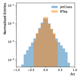
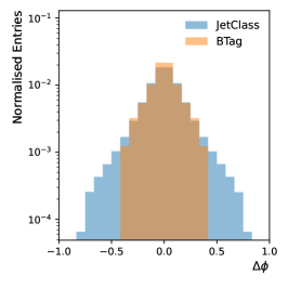
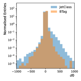
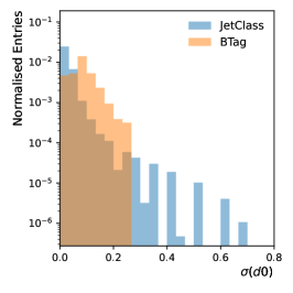
Continuous features $x^{\text{c}}$
transverse momentum	$p_{\text{T}}$
pseudorapidity to jet axis	$\Delta\eta$
azimuthal angle to jet axis	$\Delta\phi$
transverse impact parameter	$d_{0}$
longitudinal impact parameter	$z_{0}$
uncertainty on $d_{0}$	$\sigma(d_{0})$
uncertainty on $z_{0}$	$\sigma(Z_{0})$
Particle type $x^{\text{id}}$
photon	0
negative hadron	1
neutral hadron	2
positive hadron	3
electron	4
positron	5
muon	6
antimuon	7

Figure 5: The distributions of the particle features for the two datasets. The final plot shows the distributions of the particle types $x^{\text{id}}$ for the two datasets.

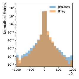
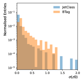
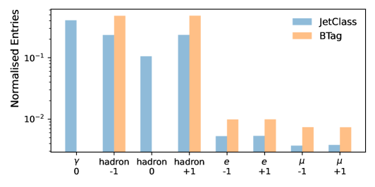
Appendix C Decoder and Mask Rate

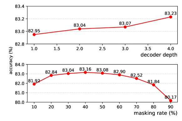
Using the K-Means + ID setup, we investigated the effect of the mask rate and the decoder depth. These results are shown in Figure 6. We found that the model was relatively robust to the mask rate but that a rate of 40% was optimal. Surprisingly at high levels of masking, 90%, the model was still able to achieve an accuracy of over 80%. We found that increasing the decoder depth improved performance, but due to computational constraints, we explored only up to 4 layers. We used these optimal settings for the final results.

Figure 6: The effect of the decoder depth (top) and the mask rate (bottom) on the classification accuracy using the outputs produced by an MPM backbone trained with the K-Means and ID tasks.

Appendix D Fixed Backbone Results

In addition to fine-tuning, we also investigate the performance of using the frozen pre-trained encoders in the same downstream tasks. The results are shown in This indicates that these backbones indeed provide a feature-rich latent space.

(a)

(b)

Figure 7: The in-distribution performance of the fixed-backbone models on the JetClass dataset. (7(a)) shows the accuracy using standard supervised classification as a function of the dataset size. (7(b)) shows the significance-improvement of the models trained in a CWoLa setting as a function of the number of signal samples in the dataset.

(a)

(b)

(c)

Figure 8: The performance of the fixed backbone models on the BTag dataset. (8(a)) shows the supervised jet classifier accuracy versus the number of samples used in fine-tuning. (8(b)) shows the ARI score for the segmentation task versus the number of secondary vertices within each jet. (8(c)) shows the balanced accuracy for the track identification task as a function of the number of tracks in each jet.

Appendix E Reconstruction Plots

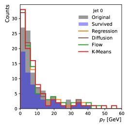
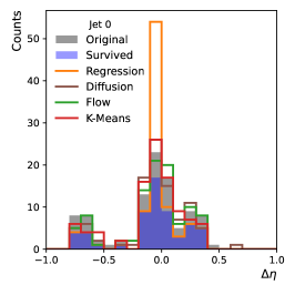
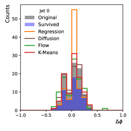
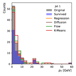
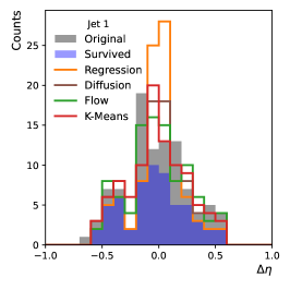
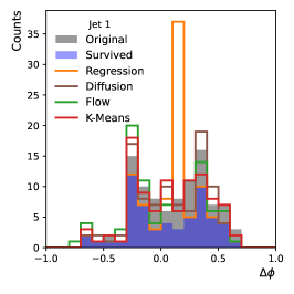
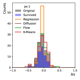
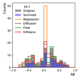
Here we show some qualitative results of some of the continuous reconstruction tasks. We select 3 jets randomly from the JetClass dataset, perform 40% masking, and then ask each backbone to reconstruct the dropped constituents. For the Regression backbone, we simply take the direct feature predictions. For the K-Means backbone, we sample under discrete distribution of centroid probabilities, then take the features of the chosen centroid. For the CNF backbone, we sample under the normalizing flow. Finally, for the CFM, we first sample from a Gaussian and then numerically integrate along the predicted trajectories. In Figure 9, we see that the Regression backbone often collapses towards the center of the distribution. This is most visible for the $\Delta\eta$ distribution of Jet-1, which clearly shows a bi-modal distribution indicative of a dual-prong jet. All other methods reconstruct this bi-modality, but the Regression backbone simply predicts the mean.

Figure 9: Reconstruction plots for the different backbones. We show 3 randomly selected jets (rows) from the JetClass dataset and plot their $(p_{\text{T}},\Delta\eta,\Delta\phi)$ distributions (columns). The grey shading shows the original jet distribution, while the blue shading shows the surviving jet distribution after 40% of the constituents were masked. The colored lines show the reconstructed jets from the different methods. The ideal reconstruction would match the original grey shape.

References

- Golling et al. [2024a] Tobias Golling et al. Masked particle modeling on sets: Towards self-supervised high energy physics foundation models. Machine Learning: Science and Technology, 2024a.
- Harris et al. [2024] Philip Harris et al. Re-simulation-based self-supervised learning for pre-training foundation models, 2024.
- Kishimoto et al. [2023] Tomoe Kishimoto et al. Pre-training strategy using real particle collision data for event classification in collider physics. In Advances in Neural Information Processing Systems, 2023.
- Vigl et al. [2024] Matthias Vigl, Nicole Hartman, and Lukas Heinrich. Finetuning foundation models for joint analysis optimization in high energy physics. Machine Learning: Science and Technology, 5(2):025075, 2024.
- Birk et al. [2024] Joschka Birk, Anna Hallin, and Gregor Kasieczka. Omnijet-: The first cross-task foundation model for particle physics, 2024.
- Mikuni and Nachman [2024] Vinicius Mikuni and Benjamin Nachman. Omnilearn: A method to simultaneously facilitate all jet physics tasks, 2024.
- Zhao et al. [2024] Zihan Zhao et al. Large-Scale Pretraining and Finetuning for Efficient Jet Classification in Particle Physics. In 22nd International Workshop on Advanced Computing and Analysis Techniques in Physics Research, 8 2024.
- Dillon et al. [2022] Barry M. Dillon et al. Symmetries, safety, and self-supervision. SciPost Phys., 12(6):188, 2022.
- Bommasani et al. [2022] Rishi Bommasani et al. On the opportunities and risks of foundation models, 2022.
- Devlin et al. [2019] Jacob Devlin et al. Bert: Pre-training of deep bidirectional transformers for language understanding, 2019.
- Radford et al. [2018] Alec Radford et al. Improving language understanding by generative pre-training, 2018.
- OpenAI [2023] OpenAI. Gpt-4 technical report, 2023.
- Lewis et al. [2019] Mike Lewis et al. Bart: Denoising sequence-to-sequence pre-training for natural language generation, translation, and comprehension, 2019.
- Brown et al. [2020] Tom Brown et al. Language models are few-shot learners. In Advances in Neural Information Processing Systems, volume 33, pages 1877–1901, 2020.
- Caron et al. [2021] Mathilde Caron et al. Emerging properties in self-supervised vision transformers. In International Conference on Computer Vision, pages 9630–9640, 2021.
- Ramesh and othersw [2021] Aditya Ramesh and othersw. Zero-shot text-to-image generation. In International Conference on Machine Learning, volume 139, pages 8821–8831, 2021.
- Alayrac et al. [2022] Jean-Baptiste Alayrac et al. Flamingo: a visual language model for few-shot learning. In Advances in Neural Information Processing Systems, volume 35, pages 23716–23736, 2022.
- Oquab et al. [2024] Maxime Oquab et al. DINOv2: Learning robust visual features without supervision. Transactions on Machine Learning Research, 2024. ISSN 2835-8856.
- He et al. [2022] Kaiming He et al. Masked autoencoders are scalable vision learners. In Conference on Computer Vision and Pattern Recognition, pages 16000–16009, 2022.
- Bao et al. [2022] Hangbo Bao et al. Beit: Bert pre-training of image transformers. In International Conference on Learning Representations, 2022.
- Agostinelli et al. [2003] S. Agostinelli et al. GEANT4: A Simulation toolkit. Nucl. Instrum. Meth. A., A506:250–303, 2003. doi: 10.1016/S0168-9002(03)01368-8.
- Vincent et al. [2008] Pascal Vincent et al. Extracting and composing robust features with denoising autoencoders. In International Conference on Machine Learning, pages 1096–1103, 2008.
- Pathak et al. [2016] Deepak Pathak et al. Context encoders: Feature learning by inpainting. In Conference on Computer Vision and Pattern Recognition, pages 2536–2544, 2016.
- Vincent et al. [2010] Pascal Vincent et al. Stacked denoising autoencoders: Learning useful representations in a deep network with a local denoising criterion. Journal of Machine Learning Research, 11(12), 2010. URL http://jmlr.org/papers/v11/vincent10a.html.
- Baevski et al. [2022] Alexei Baevski et al. Data2vec: A general framework for self-supervised learning in speech, vision and language. In International Conference on Machine Learning, pages 1298–1312, 2022.
- Wei et al. [2022] Chen Wei et al. Masked feature prediction for self-supervised visual pre-training. In Conference on Computer Vision and Pattern Recognition, pages 14668–14678, 2022.
- Xie et al. [2022] Zhenda Xie et al. Simmim: A simple framework for masked image modeling. In Conference on Computer Vision and Pattern Recognition, pages 9653–9663, 2022.
- van den Oord et al. [2017] Aaron van den Oord, Oriol Vinyals, and Koray Kavukcuoglu. Neural discrete representation learning. In Advances in Neural Information Processing Systems, volume 30, 2017.
- Chen et al. [2020] Ting Chen et al. A simple framework for contrastive learning of visual representations. In International Conference on Machine Learning, pages 1597–1607, 2020.
- de Favereau et al. [2014] J. de Favereau et al. DELPHES 3, A modular framework for fast simulation of a generic collider experiment. JHEP, 02:057, 2014.
- Qu et al. [2022] Huilin Qu, Congqiao Li, and Sitian Qian. JetClass: A Large-Scale Dataset for Deep Learning in Jet Physics, 2022. URL https://doi.org/10.5281/zenodo.6619768.
- Sjöstrand et al. [2008] Torbjörn Sjöstrand, Stephen Mrenna, and Peter Skands. A brief introduction to pythia 8.1. Comput. Phys. Commun., 178:852–867, 2008.
- Alwall et al. [2014] Johan Alwall et al. The automated computation of tree-level and next-to-leading order differential cross sections, and their matching to parton shower simulations. JHEP, 07:79, 2014.
- Cacciari et al. [2008] Matteo Cacciari, Gavin P Salam, and Gregory Soyez. The anti-kt jet clustering algorithm. JHEP, 04:063, 2008.
- CMS Collaboration [2008] CMS Collaboration. The CMS experiment at the CERN LHC. Journal of Instrumentation, 3(08):S08004, 2008. doi: 10.1088/1748-0221/3/08/S08004.
- ATLAS Collaboration [2008] ATLAS Collaboration. The ATLAS Experiment at the CERN Large Hadron Collider. Journal of Instrumentation, 3(08):S08003, 2008. doi: 10.1088/1748-0221/3/08/S08003. URL https://dx.doi.org/10.1088/1748-0221/3/08/S08003.
- ATLAS Collaboration [2020] ATLAS Collaboration. Deep Sets based Neural Networks for Impact Parameter Flavour Tagging in ATLAS. tech. report, CERN, 2020. URL https://cds.cern.ch/record/2718948.
- Yu et al. [2022] Jiahui Yu et al. Vector-quantized image modeling with improved VQGAN. In International Conference on Learning Representations, 2022.
- Omer [2021] Sehban Omer. TorchPQ, 2021. URL https://github.com/DeMoriarty/TorchPQ.
- Rezende and Mohamed [2015] Danilo Rezende and Shakir Mohamed. Variational inference with normalizing flows. In International Conference on Machine Learning, pages 1530–1538, 2015.
- Stimper et al. [2023] Vincent Stimper et al. normflows: A pytorch package for normalizing flows. Journal of Open Source Software, 8(86):5361, 2023.
- Song et al. [2020] Yang Song et al. Score-based generative modeling through stochastic differential equations, 2020.
- Karras et al. [2022] Tero Karras et al. Elucidating the design space of diffusion-based generative models, 2022.
- Lipman et al. [2023] Yaron Lipman et al. Flow matching for generative modeling. In International Conference on Learning Representations, 2023.
- Kingma et al. [2023] Diederik P. Kingma et al. Variational diffusion models, 2023.
- Sauer et al. [2024] Axel Sauer et al. Fast high-resolution image synthesis with latent adversarial diffusion distillation, 2024.
- Leigh et al. [2024] Matthew Leigh et al. Faster diffusion model with improved quality for particle cloud generation. Phys. Rev. D, 109:012010, 2024.
- Wei et al. [2023] Chen Wei et al. Diffusion models as masked autoencoders. In International Conference on Computer Vision, pages 16284–16294, 2023.
- Touvron et al. [2021] Hugo Touvron et al. Going deeper with image transformers. In International Conference on Computer Vision, pages 32–42, 2021.
- Darcet et al. [2024] Timothée Darcet et al. Vision transformers need registers. In International Conference on Learning Representations, 2024.
- Metodiev et al. [2017] Eric M Metodiev, Benjamin Nachman, and Jesse Thaler. Classification without labels: Learning from mixed samples in high energy physics. Journal of High Energy Physics, 2017(10):1–18, 2017.
- Hallin et al. [2022] Anna Hallin et al. Classifying anomalies through outer density estimation (cathode). Phys. Rev. D, 106:055006, 2022.
- Golling [2023] Tobias andothers Golling. Flow-enhanced transportation for anomaly detection. Phys. Rev. D, 107(9):096025, 2023.
- Sengupta et al. [2024a] Debajyoti Sengupta et al. Improving new physics searches with diffusion models for event observables and jet constituents. JHEP, 04:109, 2024a. doi: 10.1007/JHEP04(2024)109.
- Buhmann et al. [2024] Erik Buhmann et al. Full phase space resonant anomaly detection. Phys. Rev. D, 109(5):055015, 2024.
- Sengupta et al. [2024b] Debajyoti Sengupta et al. CURTAINs flows for flows: Constructing unobserved regions with maximum likelihood estimation. SciPost Phys., 17:046, 2024b.
- Golling et al. [2024b] Tobias Golling et al. The Interplay of Machine Learning–based Resonant Anomaly Detection Methods. Eur. Phys. J. C., 84, 03 2024b.
- Witkowski et al. [2023] Edmund Witkowski, Benjamin Nachman, and Daniel Whiteson. Learning to isolate muons in data. Phys. Rev. D, 108:092008, 2023.
- Gallicchio et al. [2011] Jason Gallicchio et al. Multivariate discrimination and the higgs+w/z search. Journal of High Energy Physics, (4):69, 2011.
- ATLAS Collaboration [2022] ATLAS Collaboration. Graph Neural Network Jet Flavour Tagging with the ATLAS Detector. tech. report, CERN, 2022. URL https://cds.cern.ch/record/2811135.
- Shlomi et al. [2021] Jonathan Shlomi et al. Secondary vertex finding in jets with neural networks. Eur. Phys. J. C, 81(6):540, 2021.
- Koch et al. [2015] Gregory Koch et al. Siamese neural networks for one-shot image recognition. In International Conference on Machine Learning, volume 2, pages 1–30, 2015.
- Hubert and Arabie [1985] Lawrence Hubert and Phipps Arabie. Comparing partitions. Journal of Classification, 2(1):193–218, 1985. doi: 10.1007/BF01908075.
- Shleifer et al. [2021] Sam Shleifer et al. Normformer: Improved transformer pretraining with extra normalization, 2021.
- Xiong et al. [2020] Ruibin Xiong et al. On layer normalization in the transformer architecture. In International Conference on Machine Learning, pages 10524–10533, 2020.
- Shazeer [2020] Noam Shazeer. Glu variants improve transformer, 2020.