Cartan moving frames and the data manifolds

Abstract

The purpose of this paper is to employ the language of Cartan moving frames to study the geometry of the data manifolds and its Riemannian structure, via the data information metric and its curvature at data points. Using this framework and through experiments, explanations on the response of a neural network are given by pointing out the output classes that are easily reachable from a given input. This emphasizes how the proposed mathematical relationship between the output of the network and the geometry of its inputs can be exploited as an explainable artificial intelligence tool.

1 Introduction

In machine learning, the idea of data manifold is based on the assumption that the data space, containing the data points on which we perform classification tasks, has a natural Riemannian manifold structure. It is a quite old concept (see [1], [2] and refs therein) and it is linked to the key question of dimensionality reduction [3], which is the key to efficient data processing for classification tasks, and more. Several geometrical tools, such as geodesics, connections, Ricci curvature, become readily available for machine learning problems under the manifold hypothesis, and are especially effective when employed in examining adversarial attacks [4, 5, 6, 7] or knowledge transfer questions, see [8, 9] and refs. therein.

More specifically, the rapidly evolving discipline of information geometry [10, 11, 12, 13] is now offering methods for discussing the above questions, once we cast them appropriately by relating the statistical manifold, i.e. the manifold of probability measures, studied in information geometry with data manifolds (see [10, 14]).

We are interested in a naturally emerging foliation structure on the data space coming through the data information matrix (DIM), which is the analog of the Fisher information matrix and in concrete experiments can be obtained by looking at a partially trained deep learning neural network for classification tasks. As it turns out, the leaves of such foliation are related with the dataset the network was trained with [14, 15]. Further work in [15] linked such study to the possible applications to knowledge transfer.

The purpose of the present paper is to study and understand the data manifolds, with Cartan moving frames method. Following the philosophy in [10], we want to equip the manifolds coming as leaves of the above mentioned foliation, via a natural metric coming through the data information matrix. As it turns out, the partial derivatives of the probabilities allow us to naturally define the Cartan moving frame at each point and are linked with the curvature of such manifold in an explicit way.

From a broader perspective, the work proposed here emphasizes the mathematical relationship between the changes in the outputs of a neural network and the curvature of the data manifolds. Furthermore, we show how this relationship can be exploited to provide explanations for the responses of a given neural network. In critical systems, providing explanations to AI model decisions can sometimes be required or mandatory by certification processes (see for example [16]). More generally, the field of eXplainable Artificial Intelligence (AI) is a fast growing research topic that develops tools for understanding and interpreting predictions given by AI models [17]. In Section 6 of this article, through simple experiments, we show how the DIM restricted to the moving frame given by the neural network output probability partial derivatives can be used to understand the local geometry of trained data. Specifically, in the case of the MNIST handwritten digits dataset [18] and CIFAR10 animals / vehicles dataset [19] by displaying the restricted DIM in the form of images, we are able to understand, starting from a given data point, which classes are easily reachable by the neural networks or not.

The organization of the paper is as follows.

In Section 2, we briefly recap some notions on information geometry and some key known results that we shall need in the sequel. Our main reference source will be [12, 13].

In Section 3, we take advantage of the machinery developed by Cartan (see [20, 21]) and define moving frames on the data manifolds via the partial derivatives of the probabilities.

In Section 4 and 5, we relate the probabilities with the curvature of the leaves, by deriving the calculations of the curvature forms in a numerically stable way.

Finally in Section 6, we consider some experiments on MNIST and CIFAR10 elucidating how near a data point, some partial derivatives of the probabilities become more important and the metric exhibits some possible singularities.

Acknowledgements. We thank Emanuele Latini, Sylvain Lavau for helpful discussions. This research was supported by Gnsaga-Indam, by COST Action CaLISTA CA21109, HORIZON-MSCA-2022-SE-01-01 CaLIGOLA, MSCA-DN CaLiForNIA - 101119552, PNRR MNESYS, PNRR National Center for HPC, Big Data and Quantum Computing, INFN Sezione Bologna. ET is grateful to the FaBiT Department of the University of Bologna for the hospitality.

2 Preliminaries

The neural networks we consider are classification functions

$$N:\mathcal{X}\times\Theta\longrightarrow\left\{p\in\mathbb{R}^{C}~{};~{}\sum_{k}p_{k}=1,~{}p_{k}>0\right\},$$

from the spaces of data $\mathcal{X}$ and weights (or parameters) $\Theta$, to the space of parameterized probability densities $p\left(y\mid x,\theta\right)$ over the set of labels $\mathcal{Y}$, where $x\in\mathcal{X}$ is the input, $y\in\mathcal{Y}$ is the target label and $\theta\in\Theta$ is the parameter of the model. For instance $\theta$ are the weights and biases in a perceptron model predicting $C$ classes, for a given input datum $x$.

We may assume both the dataspace $\mathcal{X}$ and the parameter space $\Theta$ to be (open) subsets of euclidean spaces, $\mathcal{X}\subset\mathbb{R}^{d}$, $\Theta\subset\mathbb{R}^{n}$, though it is clear that in most practical situations only a tiny portion of such open sets will be effectively occupied by data points or parameters of an actual model.

In the following, we make only two assumptions on $N$:

$$N=\mathrm{softmax}\circ s$$ (H1)

$$\forall i,j,k,\quad \partial_{x_{i}}\partial_{x_{j}}s_{k}(x)=0\quad\text{a.e.}$$ (H2)

where $s$ is called a score function, and $\mathrm{softmax}$ is the function $\left(a_{i}\right)_{i}\mapsto\left(e^{a_{i}}/\sum_{k}e^{a_{k}}\right)_{i}$. We detail why these assumptions are important in the following sections. An example of neural network satisfying these conditions is the feed-forward multi-layer perceptron with ReLU activation functions. Other popular neural network architectures verify theses assumptions.

A most important notion in information geometry is the Fisher-Rao matrix $F$, providing in some important applications, a metric on the space $\Theta$:

$$F=(f_{ij}):=\left(\mathbb{E}_{y\mid x,\theta}\left[\partial_{\theta_{i}}{\ln p(y\mid x,\theta)}\partial_{\theta_{j}}{\ln p(y\mid x,\theta)}\right]\right),\qquad 1\leq i,j\leq n.$$

We now give in analogy to $F$ the data information matrix $D$ (DIM for short), defined in a similar way.

Definition 2.1.

We define data information matrix $D=(D_{ij})$ for a point $x\in\mathcal{X}$ and a fixed model $\theta\in\Theta$ to be the following symmetric matrix:

$$D_{ij}(x)=\mathbb{E}_{y\mid x,\theta}\left[\partial_{x_{i}}{\ln p(y\mid x,\theta)}\partial_{x_{j}}{\ln p(y\mid x,\theta)}\right],\qquad 1\leq i,j\leq d.$$

Hence, $D$ is a $d\times d$ matrix, $d$ the dimension of the dataspace.

Observation 2.2.

In what follows, we will use the notation $p_{k}(x):=p\left(y_{k}\mid x,\theta\right)$ in the case of classification into a finite set $\mathcal{Y}=\left\{y_{1},\ldots,y_{C}\right\}$. We then concatenate these values in the vector $p(x)=\left(p_{k}(x)\right)_{k=1,\ldots,C}$. In practice, $p(x)=N(x)$.

We omit the dependence in $\theta$ as the parameters remain unchanged during the rest of the paper. We shall omit the dependence in $x$ too in long computations for easier reading.

As one can readily check, we have that:

$$D_{ij}(x)=\sum_{k}\frac{1}{p_{k}(x)}\partial_{x_{i}}p_{k}(x)\partial_{x_{j}}p_{k}(x).$$ (1)

In the following, we will use $\partial_{i}$, the canonical basis of $T\mathcal{X}$ associated to the coordinates $x^{i}$, and the Einstein summation notation.

Remark 2.3.

Notice the appearance of the probability $p_{i}$ at the denominator in the expression of $D$. Since $p(y\mid x,\theta)$ is an empirical probability, on data points it may happen that some of the $p_{k}(x)$ are close to zero, giving numerical instability in practical situations. We shall comment on this problem and how we may solve it, later on.

We have the following result [14], we briefly recap its proof, for completeness.

Theorem 2.4.

The data information matrix $D(x)$ is positive semidefinite, moreover

$$\ker D(x)=\left(\mathrm{span}_{k=1,\ldots,C}\left\{\sum_{i}\partial_{i}\ln p_{k}(x)\partial_{i}\right\}\right)^{\perp}$$

with $\perp$ taken w.r.t. the Euclidean scalar product on $T\mathcal{X}$. Hence, the rank of $D$ is bounded by $C-1$, with $C$ the number of classes.

Proof.

To check semipositive definiteness, let $u\in T_{x}\mathcal{X}$. Then,

$$u^{T}D(x)u =\sum_{i,j}u_{i}u_{j}\mathbb{E}_{y\mid x,\theta}\left[\partial_{i}\ln p\left(y\mid x,\theta\right)\partial_{j}\ln p\left(y\mid x,\theta\right)\right]$$

$$=\mathbb{E}_{y\mid x,\theta}\left[{\sum_{i}u_{i}\partial_{i}\ln p\left(y\mid x,\theta\right)}\sum_{j}u_{j}\partial_{j}\ln p\left(y\mid x,\theta\right)\right]$$

$$=\mathbb{E}_{y\mid x,\theta}\left[\left<\partial_{i}\ln p\left(y\mid x,\theta\right)\partial_{i},u\right>_{\mathrm{e}}^{2}\right].$$

For the statement regarding kernel and rank of $D(x)$, we notice that $u^{T}D(x)u=0$, whenever $u\in\left(\mathrm{span}_{k=1,\ldots,C}\left\{\sum_{i}\partial_{i}\ln p_{k}(x)\partial_{i}\right\}\right)^{\perp}$, where $\left<\cdot,\cdot\right>_{\mathrm{e}}$ and $\perp$ refer to the Euclidean metric. Besides, $\sum_{k}p_{k}=1\implies\sum_{ik}\partial_{i}p_{k}=0$, hence the rank bounded by $C-1$ and not $C$. ∎

This result prompts us to define the distribution:

$$x\mapsto\mathcal{D}_{x}:=\mathrm{span}\left\{\sum_{i}\partial_{i}p_{k}\left(x\right)\partial_{i},~{}k=1,\ldots,C-1\right\}.$$ (2)

For popular neural networks (satisfying H1 and H2), the distribution $\mathcal{D}$ turns to be integrable in an open set of $\mathbb{R}^{d}$, hence it defines a foliation. This matter has been discussed in [15].

Theorem 2.5.

Let $\theta$ be the weights of a neural network classifier $N$ satisfying H1 and H2, associated with the vector $p$ given by softmax. Assume $D$ has constant rank. Then, at each smooth point $x$ of $N$ there exists a local submanifold $\mathcal{L}$ of $\mathcal{X}$, such that its tangent space at $x$, $T_{x}\mathcal{L}=\mathcal{D}$.

In particular, given a dataset (e.g. MNIST), we call data leaf a leaf of such foliation containing at least one point of the dataset. In [15] the significance of such leaves is fully explored from a geometrical and experimental point of view. More specifically, Thm. 3.6 in [15] shows that the open set in Thm 2.5 is dense in the dataspace $\mathcal{X}$.

In the next sections we shall focus on the geometry of this foliation in the data space.

3 Cartan moving frames

In this section we first review some basic notions of Cartan’s approach to differentiable manifolds via the moving frames point of view and then we see some concrete application to our setting.

Definition 3.1.

Let $E\to\mathcal{L}$ be a $\mathcal{C}^{\infty}$ vector bundle over a smooth manifold $\mathcal{L}$. A connection on $E$ is a bilinear map:

$$\nabla:\mathfrak{X}\left(\mathcal{L}\right)\times\Gamma\left(E\right)\to\Gamma\left(E\right)$$

such that

$$\nabla_{v}(fs)=df(v)s+f\nabla_{v}s,\qquad v\in\mathfrak{X}\left(\mathcal{L}\right),\,f\in\mathcal{C}^{\infty}(\mathcal{L}),\,s\in\Gamma\left(E\right)$$

where $\mathfrak{X}\left(\mathcal{L}\right)$ are the vector fields on $\mathcal{L}$ and $\Gamma\left(E\right)$ the sections of the vector bundle $E$.

We shall be especially interested to the case, $E=T\mathcal{L}$ the tangent bundle to a leaf $\mathcal{L}$ of a suitable foliation (Thm. 2.5). Our framework is naturally set up to take advantange of Cartan’s language of moving frames [20]. Before we give this key definition, let us assume our distribution $\mathcal{D}$ as in (2) to be smooth, constant rank and integrable. This assumption is reasonable, since it has been shown in [15] that, for neural networks with ReLU non linearity, $\mathcal{D}$ satisfies these hypotheses in a dense open subset of the dataspace.

Definition 3.2.

We define the data foliation $\mathcal{F}_{\mathcal{D}}$, the foliation in the data space $\mathcal{X}$ defined by the distribution $\mathcal{D}$ as in Equation 2 and data leaf a leaf $\mathcal{L}_{x}$ of $\mathcal{F}$ containing at least one data point i.e. a point of the data set the network was trained with.

If $\left<\cdot,\cdot\right>_{D}$ denotes the symmetric bilinear form defined by the data information matrix $D$ as in Def. 2.1 in the dataspace, by the very definitions, when we restrict ourselves to the tangent space to a leaf $\mathcal{L}$ of $\mathcal{F}$, we have that $\left<\cdot,\cdot\right>_{\mathcal{L}}:=\left<\cdot,\cdot\right>_{D}|_{\mathcal{L}}$ is a non degenerate inner product (Prop. 2.4 and Thm. 2.5). Hence it defines a metric denoted $g^{D}$.

Definition 3.3.

Let the notation be as above and let $\mathcal{L}$ be a fixed leaf in $\mathcal{F}_{D}$. At each point $x\in\mathcal{L}$, we define $\left(e_{k}:=\sum_{i}\partial_{i}p_{k}(x)\partial_{i}\right)_{(k=1,\dots C-1)}$ to be a frame for $T_{x}\mathcal{L}$. The symmetric bilinear form $g^{D}$ defines a Riemannian metric on $\mathcal{L}$, that we call data metric.

Let $\nabla$ be the Levi-Civita connection with respect to the data information metric.

Definition 3.4.

The Levi-Civita connection

$$\nabla_{X}e_{j}=\sum_{i}\omega_{j}^{i}(X)e_{i}$$

defines $\omega_{j}^{i}$, which are called the connection forms and $\omega$ the connection matrix relative to the frame $\left(e_{i}\right)$.

The Levi-Civita connection is explicitly given by (see [20] pg 46):

$$2g^{D}\left(\nabla_{e_{a}}e_{b},e_{c}\right)=e_{a}\left(g^{D}\left(e_{b},e_{c}\right)\right)+e_{b}\left(g^{D}\left(e_{c},e_{a}\right)\right)-e_{c}\left(g^{D}\left(e_{a},e_{b}\right)\right)\\ -g^{D}\left(e_{a},\left[e_{b},e_{c}\right]\right)+g^{D}\left(e_{b},\left[e_{c},e_{a}\right]\right)+g^{D}\left(e_{c},\left[e_{a},e_{b}\right]\right).$$ (3)

To explicitly compute the connection forms $\omega_{j}^{i}(e_{k})$ we need to define

$$C_{a,b,c}:=g^{D}\left(\nabla_{e_{a}}e_{b},e_{c}\right)$$ (4)

then we have by definition that

$$C_{a,b,c}=\sum_{i}\omega^{i}_{b}\left(e_{a}\right)g^{D}\left(e_{i},e_{c}\right).$$

Define the matrix $\hat{D}=\left(g^{D}\left(e_{i},e_{j}\right)\right)_{i,j=1,\ldots,C-1}$. This is the matrix of the metric $g^{D}\left(\cdot,\cdot\right)$ restricted to a leaf $\mathcal{L}$ for the basis given by a frame. We shall see an interesting significance for the matrix $\hat{D}$ in the experiments in Section 6. Hence:

$$\sum_{i}\hat{D}_{l,i}\omega^{i}_{j}\left(e_{k}\right)=C_{k,j,l}.$$

This gives, in matrix notation:

$$\omega_{j}^{i}\left(e_{k}\right)=\left(\hat{D}^{-1}C_{k,j,\cdot}\right)_{i}.$$ (5)

The curvature tensor $R$ is given by:

$$R(X,Y)e_{j}=\sum_{i}\Omega_{j}^{i}(X,Y)e_{i}$$

where $\Omega_{j}^{i}$ is a 2-form on $T\mathcal{X}$, alternating and $\mathcal{D}$-bilinear called the curvature form (matrix) of the connection $\nabla$ relative to the frame $\left(e_{i}\right)$ on $T\mathcal{X}$.

To compute $R$ we shall make use of the following result found in [20] Theorem 11.1.

Proposition 3.5.

The curvature form $\Omega$ is given by:

$$\Omega^{i}_{j}\left(X,Y\right)=\left(d\omega^{i}_{j}\right)\left(X,Y\right)+\sum_{k}\omega^{i}_{k}\wedge\omega^{k}_{j}\left(X,Y\right).$$

By using all the previous propositions and definitions, we will see in the following sections how we can numerically compute the curvature for a neural network with a softmax function on the output.

It is useful to recall some formulae. If $\alpha$ and $\beta$ are $\mathcal{C}^{\infty}$ 1-forms and $X,Y$ are $\mathcal{C}^{\infty}$ vector fields on a manifold, then

$$\left(\alpha\wedge\beta\right)\left(X,Y\right)=\alpha(X)\beta(Y)-\alpha(Y)\beta(X)$$ (6)

and

$$\left(d\alpha\right)(X,Y)=X\alpha(Y)-Y\alpha(X)-\alpha\left(\left[X,Y\right]\right).$$ (7)

4 The Curvature of the Data Leaves

Computing in practice the curvature of a manifold with many dimensions is often intractable though essential for many tasks. This is why we are interested in computing the curvature just for the data leaves. Notice that, since in our frame $\left(e_{k}:=\sum_{i}\partial_{i}p_{k}\left(x\right)\partial_{i}\right)$, we have $\sum_{i}\partial_{i}\ln p_{k}(x)\partial_{i}=\frac{1}{p_{k}(x)}\sum_{i}{\partial_{i}p_{k}(x)\partial_{i}}=\frac{1}{p_{k}(x)}e_{k}$, we may forget the logarithm in the computations as it contributes only by a scalar factor.

Let $U=\left(\sum_{k}\partial_{k}p_{i}\partial_{k}p_{j}\right)_{i,j}$ be the matrix of the dot products of the partial derivatives of the probabilities.

With this notation, if $P=\mathrm{diag}\left\{p_{k},~{}k=1,\ldots,C\right\}$, then

$$\hat{D}_{a,b}=\left(UP^{-1}U\right)_{a,b}.$$

Besides, if $J(p)=\left(\frac{\partial p_{a}}{\partial x_{i}}\right)_{\begin{subarray}{c}a=1,\ldots,C\\ i=1,\ldots,d\end{subarray}}$ is the Jacobian matrix of first order derivatives, then $U=J(p)J(p)^{T}$.

Notice that $P$ might not be numerically invertible, whenever some classes are very unlikely and thus with a probability close to zero. The goal of this section, and the following one, is thus to derive the computations of the curvature forms in a way that is numerically stable. This will allow us to implement the curvature forms computations on a computer.

Proposition 4.1.

Let the notation be as above. We have:

$$\left[e_{a},e_{b}\right]={H}\left(p_{b}\right)e_{a}-{H}\left(p_{a}\right)e_{b}$$ (8)

with ${H}\left(f\right)=\left(\partial_{i}\partial_{j}f\right)_{i,j=1,\ldots,d}$ the matrix of second order partial derivatives.

Proof.

First, recall that $\left[u^{k}\partial_{k},v^{l}\partial_{l}\right]=\left(u^{k}\frac{\partial v^{l}}{\partial x^{k}}-v^{k}\frac{\partial u^{l}}{\partial x^{k}}\right)\partial_{l}$. Thus, with $u^{k}=\frac{\partial p_{a}}{\partial x^{k}}$ and $v^{l}=\frac{\partial p_{b}}{\partial x^{l}}$ we get:

$$\left[e_{a},e_{b}\right] =\left(\sum_{k}\frac{\partial p_{a}}{\partial x^{k}}\frac{\partial^{2}p_{b}}{\partial x^{k}\partial x^{l}}-\sum_{k}\frac{\partial p_{b}}{\partial x^{k}}\frac{\partial^{2}p_{a}}{\partial x^{k}\partial x^{l}}\right)\partial_{l}$$

$$={H}\left(p_{b}\right)e_{a}-{H}\left(p_{a}\right)e_{b}.$$

∎

Proposition 4.2.

If $s$ represent the score vector, i.e. the output of the neural network before going through the softmax function then, for all $j=1,\ldots,C$,

$$\partial_{j}p_{i}=\sum_{k}p_{i}\left(\delta_{ik}-p_{k}\right)\partial_{j}s_{k}\quad\text{and}\quad\partial_{j}\ln p_{i}=\sum_{k}\left(\delta_{ik}-p_{k}\right)\partial_{j}s_{k}.$$ (9)

In term of Jacobian matrices, this rewrites as

$$J\left(p\right)=\left(P-pp^{T}\right)J\left(s\right).$$

Proof.

This is simply due to the fact that $p=\mathrm{softmax}\left(s\right)$ and that the derivative of the softmax function is $\frac{\partial\textrm{softmax}(x)_{i}}{\partial x_{k}}=\textrm{softmax}(x)_{i}\left(\delta_{i,k}-\textrm{softmax}(x)_{k}\right)$. ∎

We now give other formulae for the second order partial derivatives of the probabilities.

Proposition 4.3.

Let the notation be as above. We have:

$${H}\left(p_{a}\right)_{ij}=\frac{\partial_{i}p_{a}\partial_{j}p_{a}}{p_{a}}-p_{a}\sum_{k=1}^{C}\partial_{i}p_{k}\partial_{j}s_{k}.$$ (10)

Proof.

$${H}\left(p_{a}\right)_{ij} =\partial_{i}\left(\partial_{j}p_{a}\right)=\partial_{i}\left(\sum_{k}p_{a}\left(\delta_{ik}-p_{k}\right)\partial_{j}s_{k}\right)$$

$$=\partial_{i}p_{a}\underbrace{\sum_{k}\left(\delta_{ak}-p_{k}\right)\partial_{j}s_{k}}_{=\frac{1}{p_{a}}\partial_{j}p_{a}}+p_{a}\sum_{k}\partial_{i}\left(\left(\delta_{ak}-p_{k}\right)\partial_{j}s_{k}\right)$$

$$=\frac{1}{p_{a}}\partial_{i}p_{a}\partial_{j}p_{a}+p_{a}\sum_{k}\left(\delta_{ak}-p_{k}\right){H}\left(s_{k}\right)-p_{a}\sum_{k}\partial_{i}p_{k}\partial_{j}s_{k}.$$

But ${H}\left(s_{k}\right)=0$ almost everywhere by H2. ∎

However, with this form, the probability at the denominator will cause some instability problems, whenever the network is sufficiently trained. Thus, we express ${H}\left(p_{a}\right)$ in another form below.

Proposition 4.4.

Let the notation be as above. We have:

$${H}\left(p_{a}\right)_{ij} =\sum_{k}\left[\left(\delta_{ak}-p_{k}\right)\partial_{i}p_{a}-p_{a}\partial_{i}p_{k}\right]\partial_{j}s_{k}$$

$$=p_{a}\sum_{k}\left[\left(\delta_{ak}-p_{k}\right)\sum_{l}\left(\delta_{al}-p_{l}\right)\partial_{i}s_{l}-\partial_{i}p_{k}\right]\partial_{j}s_{k}.$$

Proof.

The proof is a straightforward combination of Equation 9 and Equation 10. We simply need to replace $\partial_{i}p_{a}$ twice in the expression 10 by 9. ∎

Lemma 4.5.

$$e_{a}\left(D\right)(x)=J(s)^{T}A_{a}J(s)$$ (11)

with

$$\left(A_{a}\right)_{kl}=\sum_{i}\partial_{i}p_{a}\left(\left(\delta_{kl}-p_{l}\right)\partial_{i}p_{k}-p_{k}\partial_{i}p_{l}\right)$$

Proof.

$$e_{a}\left(D\right)(x) =\sum_{i}\partial_{i}p_{a}\partial_{i}D(x)$$

$$=\sum_{i}\partial_{i}p_{a}\partial_{i}\left(J(s)^{T}\left(P-pp^{T}\right)J(s)\right)$$

$$=\sum_{i}\partial_{i}p_{a}J(s)^{T}\partial_{i}\left(P-pp^{T}\right)J(s)\quad\text{because }{H}\left(s_{k}\right)=0.$$

Indeed, ${H}\left(s_{k}\right)=0$ for all $k$ almost everywhere by H2. Then at the indexes $k,l$, we get:

$$\partial_{i}\left(P-pp^{T}\right)_{kl} =\partial_{i}\left(p_{k}\delta_{kl}-p_{k}p_{l}\right)$$

$$=\delta_{kl}\partial_{i}p_{k}-p_{l}\partial_{i}p_{k}-p_{k}\partial_{i}p_{l}.$$

Thus, by multiplying with $\partial_{i}p_{a}$ and summing over $i$, it gives the expression of $A_{a}$. ∎

Proposition 4.6.

Recall that the neural network satisfies H2, then

$$e_{a}\left(g^{D}\left(e_{b},e_{c}\right)\right) =M_{a,c,b}+M_{a,b,c}+\left(J(s)e_{b}\right)^{T}A_{a}J(s)e_{c}$$

with

$$M_{a,b,c} =\left({H}\left(p_{b}\right)e_{a}\right)^{T}J(s)^{T}\left(P-pp^{T}\right)J(s)e_{c}.$$

Proof.

The proof is straightforward.

$$e_{a}\left(g^{D}\left(e_{b},e_{c}\right)\right) =\sum_{i}\partial_{i}p_{a}\partial_{i}\left(e_{b}^{T}D(x)e_{c}\right)$$

$$=\sum_{i}\partial_{i}p_{a}\partial_{i}\left(e_{b}^{T}\right)D(x)e_{c}+\sum_{i}\partial_{i}p_{a}e_{b}^{T}\partial_{i}\left(D(x)\right)e_{c}$$

$$\qquad+\sum_{i}\partial_{i}p_{a}e_{b}^{T}D(x)\partial_{i}e_{c}$$

$$=e_{a}^{T}{H}\left(p_{b}\right)^{T}D(x)e_{c}+e_{b}^{T}e_{a}\left(D(x)\right)e_{c}+e_{b}^{T}D(x){H}\left(p_{c}\right)e_{a}$$

$$=M_{a,b,c}+e_{b}^{T}J(s)^{T}A_{a}J(s)e_{c}+\left(e_{a}^{T}{H}\left(p_{c}\right)^{T}D(x)e_{b}\right)^{T}$$

$$=M_{a,b,c}+e_{b}^{T}J(s)^{T}A_{a}J(s)e_{c}+\left(M_{a,c,b}\right)^{T}.$$

And $M_{a,c,b}$ is a scalar, thus $M_{a,c,b}^{T}=M_{a,c,b}$, hence the result. ∎

Then, we use the following proposition to remove the second order derivative in $M$. An alternative formula for this expression is given in A.1. This facilitates the computations with automatic differentiation methods.

Proposition 4.7.

$${H}\left(p_{a}\right)e_{b}=\left(\sum_{k,i}\left(\delta_{ak}-p_{k}\right)\left(\partial_{i}s_{k}\partial_{i}p_{b}\right)\right)e_{a}-\sum_{k,i}p_{a}\left(\partial_{i}s_{k}\partial_{i}p_{b}\right)e_{k}.$$ (12)

Proof.

$${H}\left(p_{a}\right)e_{b} =\sum_{i}\left(\sum_{k}\left(\left(\delta_{ak}-p_{k}\right)\partial_{j}p_{a}-p_{a}\partial_{j}p_{k}\right)\partial_{i}s_{k}\right)\partial_{i}p_{b}$$

$$=\sum_{i}\left(\sum_{k}\left(\delta_{ak}-p_{k}\right)\partial_{j}p_{a}\partial_{i}s_{k}\right)\partial_{i}p_{b}-p_{a}\sum_{i}\left(\sum_{k}\partial_{j}p_{k}\partial_{i}s_{k}\right)\partial_{i}p_{b}$$

$$=\left(\sum_{k,i}\left(\delta_{ak}-p_{k}\right)\partial_{i}s_{k}\partial_{i}p_{b}\right)\partial_{j}p_{a}-p_{a}\sum_{k,i}\left(\partial_{i}s_{k}\partial_{i}p_{b}\right)\partial_{j}p_{k}.$$

∎

Proposition 4.8.

$$g^{D}\left(e_{a},\left[e_{b},e_{c}\right]\right)=\sum_{i,j,k}\partial_{i}p_{a}D(x)_{ij}\left(\partial_{j}\partial_{k}{p_{c}}\partial_{k}p_{b}-\partial_{j}\partial_{k}{p_{b}}\partial_{k}p_{c}\right).$$ (13)

Proof.

Straightforward from the previous propositions and lemmas. ∎

With all these propositions, the connection forms can be computed directly without numerical instabilities.

5 Computation of the curvature forms

In this section we conclude our calculation of the curvature forms. In Prop. 3.5 we wrote the explicit expression for the curvature form as:

$$\Omega\left(X,Y\right)=\left(d\omega\right)\left(X,Y\right)+\omega\wedge\omega\left(X,Y\right).$$ (14)

where $\omega$ denotes the (Levi-Civita) connection form. To ease the reading we go back to notation of Section 3 and we set:

$$e_{k}:=\sum_{i}\partial_{i}p_{k}\left(x\right)\partial_{i},\quad\hbox{for}\quad k=1,\dots,C-1.$$

We then can express explicitly the connection form as:

$$\nabla_{X}e_{j}=\sum\omega_{j}^{i}(X)e_{i}.$$

The wedge product of the connection forms in (14) can thus be easily computed with the propositions of the previous section, because of formula (6) report here:

$$\left(\omega\wedge\omega\right)\left(X,Y\right)=\omega(X)\omega(Y)-\omega(Y)\omega(X).$$ (15)

The exterior derivative of $\omega$ remains to be computed and it is more complicated. We recall the formula (7):

$$\left(d\omega\right)(X,Y)=X\omega(Y)-Y\omega(X)-\omega\left(\left[X,Y\right]\right).$$ (16)

The last term is computed via the following proposition.

Proposition 5.1.

Let the notation be as above. Then:

$$\omega_{j}^{i}\left(\left[e_{a},e_{b}\right]\right)= \left(\sum_{k,l}\left(\delta_{bk}-p_{k}\right)\left(\partial_{l}s_{k}\partial_{l}p_{a}\right)\right)\omega_{j}^{i}\left(e_{b}\right)$$

$$-\left(\sum_{k,l}\left(\delta_{ak}-p_{k}\right)\left(\partial_{l}s_{k}\partial_{l}p_{b}\right)\right)\omega_{j}^{i}\left(e_{a}\right)$$

$$-\sum_{k,l}\left(\partial_{l}s_{k}\left(p_{b}\partial_{l}p_{a}-p_{a}\partial_{l}p_{b}\right)\right)\omega_{j}^{i}\left(e_{k}\right).$$

Proof.

$$\omega_{j}^{i}\left(\left[e_{a},e_{b}\right]\right) =\omega_{j}^{i}\left({H}\left(p_{b}\right)e_{a}\right)-\omega_{j}^{i}\left({H}\left(p_{a}\right)e_{b}\right).$$

Besides,

$$\omega_{j}^{i}\left({H}\left(p_{a}\right)e_{b}\right) =\omega_{j}^{i}\left(\left(\sum_{k,l}\left(\delta_{ak}-p_{k}\right)\left(\partial_{l}s_{k}\partial_{l}p_{b}\right)\right)e_{a}-\sum_{k,l}p_{a}\left(\partial_{l}s_{k}\partial_{l}p_{b}\right)e_{k}\right)$$

$$=\left(\sum_{k,l}\left(\delta_{ak}-p_{k}\right)\left(\partial_{l}s_{k}\partial_{l}p_{b}\right)\right)\omega_{j}^{i}\left(e_{a}\right)-\sum_{k,l}p_{a}\left(\partial_{l}s_{k}\partial_{l}p_{b}\right)\omega_{j}^{i}\left(e_{k}\right).$$

Thus,

$$\omega_{j}^{i}\left(\left[e_{a},e_{b}\right]\right)= \left(\sum_{k,l}\left(\delta_{bk}-p_{k}\right)\left(\partial_{l}s_{k}\partial_{l}p_{a}\right)\right)\omega_{j}^{i}\left(e_{b}\right)$$

$$-\left(\sum_{k,l}\left(\delta_{ak}-p_{k}\right)\left(\partial_{l}s_{k}\partial_{l}p_{b}\right)\right)\omega_{j}^{i}\left(e_{a}\right)$$

$$-\sum_{k,l}\left(\partial_{l}s_{k}\left(p_{b}\partial_{l}p_{a}-p_{a}\partial_{l}p_{b}\right)\right)\omega_{j}^{i}\left(e_{k}\right).$$

∎

We now tackle the question of determining the first two terms in (7).

Observation 5.2.

We notice that to compute $e_{a}\left(\omega^{i}_{j}\left(e_{b}\right)\right)$, we can use the fact that:

$$e_{a}\left(g^{D}\left(\nabla_{e_{b}}e_{c},e_{d}\right)\right) =e_{a}\left(\sum_{i}\omega_{c}^{i}\left(e_{b}\right)g^{D}\left(e_{i},e_{d}\right)\right)$$

$$=\sum_{i}e_{a}\left(\omega_{c}^{i}\left(e_{b}\right)\right)g^{D}\left(e_{i},e_{d}\right)+\sum_{i}\omega_{c}^{i}\left(e_{b}\right)e_{a}\left(g^{D}\left(e_{i},e_{d}\right)\right)$$

$$\iff\sum_{i}\hat{D}_{d,i}e_{a}\left(\omega_{c}^{i}\left(e_{b}\right)\right) =\underbrace{e_{a}\left(g^{D}\left(\nabla_{e_{b}}e_{c},e_{d}\right)\right)-\sum_{i}\omega_{c}^{i}\left(e_{b}\right)e_{a}\left(g^{D}\left(e_{i},e_{d}\right)\right)}_{N_{a,b,c,d}}$$

$$\iff e_{a}\left(\omega_{c}^{\cdot}\left(e_{b}\right)\right) =\hat{D}^{-1}N_{a,b,c,\cdot}.$$

Hence we need to compute: $e_{a}g^{D}\left(\nabla_{e_{b}}e_{c},e_{d}\right)$.

Theorem 5.3.

The expression of the curvature is given by:

$$\Omega^{i}_{j}\left(e_{a},e_{b}\right)={\left(\hat{D}^{-1}N_{a,b,j,\cdot}\right)_{i}-\left(\hat{D}^{-1}N_{b,a,j,\cdot}\right)_{i}-\omega^{i}_{j}\left(\left[e_{a},e_{b}\right]\right)}\\ +\sum_{k}\left[\omega^{i}_{k}\left(e_{a}\right)\omega^{k}_{j}\left(e_{b}\right)-\omega^{i}_{k}\left(e_{b}\right)\omega^{k}_{j}\left(e_{a}\right)\right]$$ (17)

where $N_{a,b,c,\cdot}=\left(N_{a,b,c,d}\right)_{d=1,\ldots,C-1}$ is the vector defined in Observation 5.2 by $e_{a}\left(g^{D}\left(\nabla_{e_{b}}e_{c},e_{d}\right)\right)-\sum_{i}\omega_{c}^{i}\left(e_{b}\right)e_{a}\left(g^{D}\left(e_{i},e_{d}\right)\right)$ for $d=1,\ldots,C-1$, and where $\hat{D}=\left(g^{D}\left(e_{i},e_{j}\right)\right)_{i,j=1,\ldots,C-1}$ is the matrix of pairwise metric products of the frame.

We report the lemmas needed to compute the tensor $N_{a,b,c,d}$ in Appendix B.

6 Experiments

To understand why the frame $e_{a}=\sum_{i}\partial_{i}p_{a}\partial_{i}$ and the DIM were chosen to compute the connection and curvature forms, we shall focus on experiments on the MNIST and the CIFAR10 datasets. As we will see, this frame and the DIM can provide some explanations to the response of the neural network.

The MNIST dataset is composed of 60k train images of shape $28\times 28$ pixels depicting handwritten digits between $0$ and $9$, and the CIFAR10 dataset is composed of 60k RGB train images of shape $32\times 32$ classified in 10 different classes (see Table 1).

Table 1: Correspondence index - class of the CIFAR10 dataset.

No.	0	1	2	3	4	5	6	7	8	9
Class	airplane	automobile	bird	cat	deer	dog	frog	horse	ship	truck

On Figure 1 are represented various input points $x$ from the MNIST training set and the corresponding matrix $\hat{D}_{x}=\left(g_{x}\left(e_{a},e_{b}\right)\right)_{a,b=1,\ldots,C}$. The neural network used in this experiment is defined as stated in Table 2. This network has been trained on the test set of MNIST with stochastic gradient descent until convergence (98% accuracy on the test set).

On Figure 1, it can be seen that the matrices $\hat{D}_{x}$ have only a few main components indicating which probabilities are the easiest to change. A large (positive) component on the diagonal at index $i$ suggests that one can increase or decrease easily $p_{i}(x)$ by moving in the directions $\pm e_{i}$. A negative (resp. positive) component at position $(i,j)$ indicates that, starting from the image $x$, classes $i$ and $j$ are in opposite (resp. the same) directions: increasing $p_{i}(x)$ will most likely decrease (resp. increase) $p_{j}(x)$.

For instance, the first image on the top left is correctly classified as a 2 by the network, but since the coefficient $(3,3)$ of matrix $\hat{D}$ is positive too, it indicates that class 3 should be easily reachable. This makes sense, as the picture can also be interpreted as a part of the 3 digit. Negative coefficients at $(3,2)$ and $(2,3)$ thus indicates that going in the direction of a 3 will decrease the probability of predicting a 2. On the second picture, the same phenomenon arises but with classes 2 and 8. Indeed, the buckle in the bottom part of the picture brings it closer to an 8.

Remark 6.1.

Be careful as teal colored coefficients on Figure 1 and Figure 2 are not exactly zero but rather very low compared to the few main ones that are yellow and purple.

Table 2: Architecture of the neural network trained on MNIST.

No.	Layers (sequential)
(0):	Conv2d(1, 32, kernel_size=(3, 3), stride=(1, 1))
(1):	ReLU()
(2):	Conv2d(32, 64, kernel_size=(3, 3), stride=(1, 1))
(3):	ReLU()
(4):	MaxPool2d(kernel_size=2, stride=2, padding=0, dilation=1)
(5):	Flatten()
(6):	Linear(in_features=9216, out_features=128, bias=True)
(7):	ReLU()
(8):	Linear(in_features=128, out_features=10, bias=True)
(9):	Softmax()

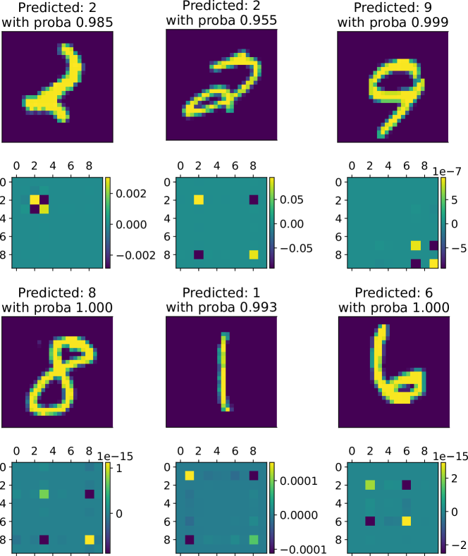
Figure 1: Couples of input point $x$ (above) and the corresponding matrix $\hat{D}(x)=\left(g^{D}_{x}\left(e_{a},e_{b}\right)\right)_{a,b=1,\ldots,C}$ (below) on MNIST.

On Figure 2 are represented various input points $x$ from the CIFAR10 training set and the corresponding matrix $\hat{D}_{x}=\left(g_{x}\left(e_{a},e_{b}\right)\right)_{a,b=1,\ldots,C}$. The neural network used in this experiment is defined as stated in Table 3. This network has been trained on the test set of CIFAR10 with stochastic gradient descent until convergence (84% accuracy on the test set).

On Figure 2, it can be seen that the matrices $\hat{D}_{x}$ have only a few main components indicating which probabilities are the easiest to change, i.e. with a similar behavior as seen above for MNIST. The interpretation of matrix $\hat{D}$ then is identical.

For instance, the first image on the top left is correctly classified as a dog (class No. 5) by the network, but since the coefficient $(3,3)$ of matrix $\hat{D}$ is positive too, it indicates that class No. 3 “cat” should be easily reachable. This makes sense since dogs and cats form a subclass of similar little animals. Negative coefficients at $(3,2)$ and $(2,3)$ thus indicates that going in the direction of the cat will decrease the probability of predicting a dog. There are also positive coefficients at $(3,7)$ and $(7,3)$ indicating that going in the direction of the cat should also slightly increase the probability of seeing a horse. Again, this makes sense as they all belong in the animal subclass.

On the second picture, the dog can be transformed into a cat or a frog, probably because of the green cloth around its neck.

Table 3: Architecture of the neural network trained on CIFAR10.

No.	Layers (sequential)
(0):	Conv2d(3, 64, kernel_size=(3, 3), stride=(1, 1), padding=(1, 1))
(1):	BatchNorm2d(64, eps=1e-05, momentum=0.1)
(2):	ReLU()
(3):	MaxPool2d(kernel_size=2, stride=2, padding=0, dilation=1)
(4):	Conv2d(64, 128, kernel_size=(3, 3), stride=(1, 1), padding=(1, 1))
(5):	BatchNorm2d(128, eps=1e-05, momentum=0.1)
(6):	ReLU()
(7):	MaxPool2d(kernel_size=2, stride=2, padding=0, dilation=1)
(8):	Conv2d(128, 256, kernel_size=(3, 3), stride=(1, 1), padding=(1, 1))
(9):	BatchNorm2d(256, eps=1e-05, momentum=0.1)
(10):	ReLU()
(11):	Conv2d(256, 256, kernel_size=(3, 3), stride=(1, 1), padding=(1, 1))
(12):	BatchNorm2d(256, eps=1e-05, momentum=0.1)
(13):	ReLU()
(14):	MaxPool2d(kernel_size=2, stride=2, padding=0, dilation=1, ceil mode=False)
(15):	Conv2d(256, 512, kernel_size=(3, 3), stride=(1, 1), padding=(1, 1))
(16):	BatchNorm2d(512, eps=1e-05, momentum=0.1)
(17):	ReLU()
(18):	Conv2d(512, 512, kernel_size=(3, 3), stride=(1, 1), padding=(1, 1))
(19):	BatchNorm2d(512, eps=1e-05, momentum=0.1)
(20):	ReLU()
(21):	MaxPool2d(kernel_size=2, stride=2, padding=0, dilation=1, ceil mode=False)
(22):	Conv2d(512, 512, kernel_size=(3, 3), stride=(1, 1), padding=(1, 1))
(23):	BatchNorm2d(512, eps=1e-05, momentum=0.1)
(24):	ReLU()
(25):	Conv2d(512, 512, kernel_size=(3, 3), stride=(1, 1), padding=(1, 1))
(26):	BatchNorm2d(512, eps=1e-05, momentum=0.1)
(27):	ReLU()
(28):	MaxPool2d(kernel_size=2, stride=2, padding=0, dilation=1, ceil mode=False)
(29):	AvgPool2d(kernel_size=1, stride=1, padding=0)
(30):	Linear(in_features=512, out_features=10, bias=True)
(31):	Softmax(dim=1)

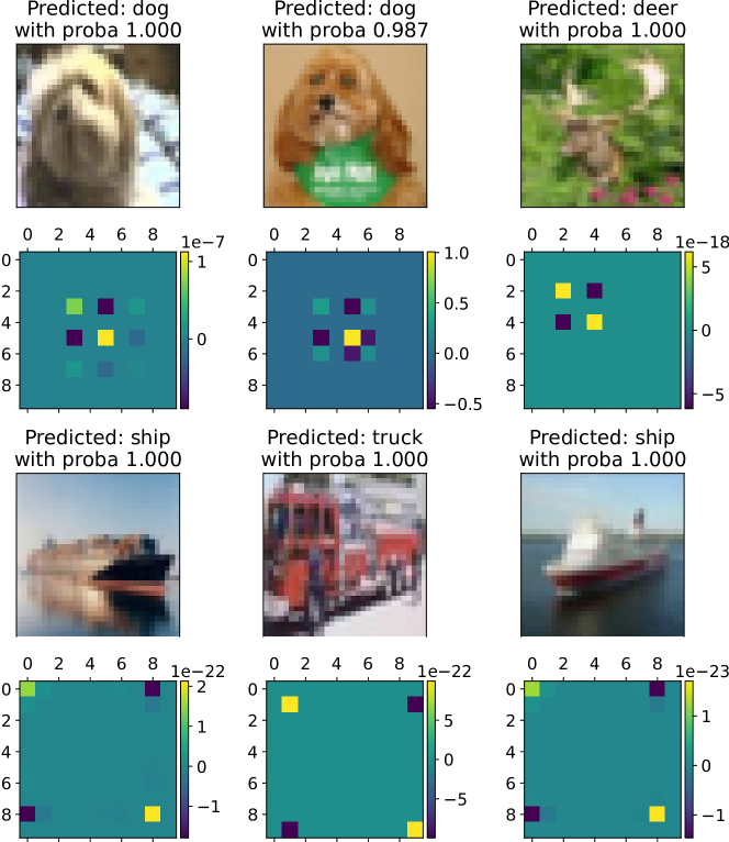
Figure 2: Couples of input point $x$ (above) and the corresponding matrix $\hat{D}(x)=\left(g^{D}_{x}\left(e_{a},e_{b}\right)\right)_{a,b=1,\ldots,C}$ (below) on CIFAR10.

7 Conclusion

In this study, we have shown that analyzing the geometry of the data manifold of a neural network using Cartan moving frames is natural and practical. Indeed, from the Fisher Information Matrix, we define a corresponding Data Information Matrix that generates a foliation structure in the data space. The partial derivatives of the probabilities learned by the neural network define a Cartan moving frame on the leaves of the data manifold. We detail how the moving frame can be used as a tool to provide some explanations on the classification changes that can easily happen or not around a given data point. Experiments on the MNIST and CIFAR datasets confirm the relevance of the explanations provided by the Cartan moving frames and the corresponding Date Information Matrix. For very large neural network, the theory still holds. However, the method might be limited by the computational requirements of the partial derivatives calculation for each class (usually obtained through automatic differentiation). We believe that combining the moving frame, the connection and the curvature forms should provide new insights to build more advanced explainable AI tools. This is work in progress.

Appendix A An auxiliary lemma

We report here, for convenience, an alternative formula for the expression used in 4.6.

Proposition A.1.

Recall that $U=\left(u_{i,j}\right)=\left(\left<e_{i},e_{j}\right>_{\mathrm{e}}\right)_{i,j}$. Then

$$e_{a}\left(g^{D}\left(e_{b},e_{c}\right)\right)=\quad \sum_{j}u_{aj}u_{bj}u_{cj}\frac{1}{p_{j}^{2}}$$

$$+ \left(\frac{u_{ab}}{p_{b}}+\frac{u_{ac}}{p_{c}}\right)\sum_{j}\frac{1}{p_{j}}u_{bj}u_{cj}$$

$$- \sum_{j}\left(u_{cj}p_{b}+u_{bj}p_{c}\right)\frac{1}{p_{j}}\sum_{k,i}\left(\partial_{i}p_{a}\partial_{i}s_{k}\right)u_{jk}$$

$$- \sum_{i}\left(\partial_{i}p_{a}\partial_{i}s_{k}\right)\left(u_{cj}u_{bk}+u_{bj}u_{ck}\right).$$

Notice that on the second line, we recognise the expression of $g^{D}\left(e_{b},e_{c}\right)$ for the sum.

Proof.

$$e_{a}\left(g^{D}\left(e_{b},e_{c}\right)\right) =\sum_{i}\partial_{i}p_{a}\partial_{i}\left(g^{D}\left(e_{b},e_{c}\right)\right)$$

$$=\sum_{i}\partial_{i}p_{a}\partial_{i}\left(\sum_{j}\frac{1}{p_{j}}u_{bj}u_{cj}\right)$$

$$=\sum_{i,j}\partial_{i}p_{a}\left(\left(\partial_{i}\frac{1}{p_{j}}\right)u_{cj}u_{bj}+\frac{1}{p_{j}}\left(\partial_{i}u_{bj}\right)u_{cj}+\frac{1}{p_{j}}u_{bj}\left(\partial_{i}u_{cj}\right)\right).$$

Now we compute $\partial_{i}u_{bj}$ :

$$\partial_{i}u_{bj} =\partial_{i}\left(\sum_{l}\partial_{l}p_{b}\partial_{l}p_{j}\right)$$

$$=\sum_{l}\underbrace{\left(\partial_{i}\partial_{l}p_{b}\right)}_{={H}\left(p_{b}\right)_{i,l}}\partial_{l}p_{j}+\sum_{l}\partial_{l}p_{b}\left(\partial_{i}\partial_{l}p_{j}\right)$$

$$=\sum_{l}\left(\frac{\partial_{i}p_{b}\partial_{l}p_{b}}{p_{b}}-p_{b}\sum_{k}\partial_{i}s_{k}\partial_{l}p_{k}\right)\partial_{l}p_{j}$$

$$\quad+\sum_{l}\partial_{l}p_{b}\left(\frac{\partial_{i}p_{j}\partial_{l}p_{j}}{p_{j}}-p_{j}\sum_{k}\partial_{i}s_{k}\partial_{l}p_{k}\right)$$

$$=\sum_{l}\left(\frac{\partial_{i}p_{b}}{p_{b}}+\frac{\partial_{i}p_{j}}{p_{j}}\right)u_{aj}-\sum_{l}\left(p_{a}\partial_{l}p_{j}+p_{j}\partial_{l}p_{a}\right)\sum_{k}\partial_{i}s_{k}\partial_{l}p_{k}.$$

Thus

$$e_{a}\left(g^{D}\left(e_{b},e_{c}\right)\right)=\quad \sum_{j}u_{bj}u_{cj}u_{aj}\frac{-1}{p_{j}^{2}}$$

$$+ \sum_{j}\left(\frac{u_{ab}}{p_{b}}+\frac{u_{aj}}{p_{j}}\right)\frac{1}{p_{j}}u_{bj}u_{cj}$$

$$- \sum_{j}\frac{1}{p_{j}}u_{cj}\left(p_{b}\sum_{k,l}\left(\partial_{l}p_{a}\partial_{l}s_{k}\right)u_{jk}+p_{j}\sum_{k,l}\left(\partial_{l}p_{a}\partial_{l}s_{k}\right)u_{bk}\right)$$

$$+ \sum_{j}\left(\frac{u_{ac}}{p_{c}}+\frac{u_{aj}}{p_{j}}\right)\frac{1}{p_{j}}u_{bj}u_{cj}$$

$$- \sum_{j}\frac{1}{p_{j}}u_{bj}\left(p_{c}\sum_{k,l}\left(\partial_{l}p_{a}\partial_{l}s_{k}\right)u_{jk}+p_{j}\sum_{k,l}\left(\partial_{l}p_{a}\partial_{l}s_{k}\right)u_{ck}\right).$$

∎

To get a numerically stable expression for $e_{a}g^{D}\left(e_{b},e_{c}\right)$, we can develop $u$ with Equation 9 and the probability at the denominator will cancel out with the one in factor of Equation 9.

Appendix B Further computations of the curvature forms

In this section we report, for convenience, some lemmas necessary for the full derivation of the curvature forms calculations.

Lemma B.1.

$$e_{a}\left(e_{b}\left(g^{D}\left(e_{c},e_{d}\right)\right)\right)=e_{a}\left(M_{b,d,c}\right)+e_{a}\left(M_{b,c,d}\right)+e_{a}\left(e_{c}^{T}J(s)^{T}A_{b}J(s)e_{d}\right).$$ (18)

Proof.

$$e_{a}\left(e_{b}\left(g^{D}\left(e_{c},e_{d}\right)\right)\right) =e_{a}\left(M_{b,d,c}+M_{b,c,d}+e_{c}^{T}J(s)^{T}A_{b}J(s)e_{d}\right)$$

$$=e_{a}\left(M_{b,d,c}\right)+e_{a}\left(M_{b,c,d}\right)+e_{a}\left(e_{c}^{T}J(s)^{T}A_{b}J(s)e_{d}\right).$$

∎

Lemma B.2.

$$e_{a}\left(M_{b,c,d}\right)=~{}e_{a}\left({H}\left(p_{c}\right)e_{b}\right)^{T}D(x)e_{d}\\ +\left({H}\left(p_{c}\right)e_{b}\right)^{T}J(s)^{T}A_{a}J(s)e_{d}\\ +\left({H}\left(p_{c}\right)e_{b}\right)^{T}D(x)\left({H}\left(p_{d}\right)e_{a}\right).$$ (19)

Proof.

$$e_{a}\left(M_{b,c,d}\right)= ~{}e_{a}\left(e_{b}^{T}{H}\left(p_{c}\right)^{T}D(x)e_{d}\right)$$

$$= ~{}e_{a}\left({H}\left(p_{c}\right)e_{b}\right)^{T}D(x)e_{d}$$

$$+\left({H}\left(p_{c}\right)e_{b}\right)^{T}e_{a}\left(D(x)\right)e_{d}$$

$$+\left({H}\left(p_{c}\right)e_{b}\right)^{T}D(x)e_{a}\left(e_{d}\right)$$

$$= ~{}e_{a}\left({H}\left(p_{c}\right)e_{b}\right)^{T}D(x)e_{d}$$

$$+\left({H}\left(p_{c}\right)e_{b}\right)^{T}J(s)^{T}A_{a}J(s)e_{d}$$

$$+\left({H}\left(p_{c}\right)e_{b}\right)^{T}D(x)\left({H}\left(p_{d}\right)e_{a}\right).$$

∎

Lemma B.3.

$$e_{a}\left({H}\left(p_{c}\right)e_{b}\right)= ~{}\sum_{k}\Big{[}-\left(u_{ak}\right)\left(\sum_{i}\partial_{i}s_{k}\partial_{i}p_{b}\right)e_{c}$$

$$\qquad+\left(\delta_{ck}-p_{k}\right)\left(\sum_{i,j}\partial_{i}s_{k}\partial_{i}\partial_{j}p_{b}\partial_{j}p_{a}\right)e_{c}$$

$$\qquad+\left(\delta_{ck}-p_{k}\right)\left(\sum_{i}\partial_{i}s_{k}\partial_{i}p_{b}\right){H}\left(p_{c}\right)e_{a}\Big{]}$$

$$~{}-\sum_{k}\Big{[}\left(u_{ac}\right)\left(\sum_{i}\partial_{i}s_{k}\partial_{i}p_{b}\right)e_{k}$$

$$\qquad+p_{c}\left(\sum_{i,j}\partial_{i}s_{k}\partial_{i}\partial_{j}p_{b}\partial_{j}p_{a}\right)e_{k}$$

$$\qquad+p_{c}\left(\sum_{i}\partial_{i}s_{k}\partial_{i}p_{b}\right){H}\left(p_{k}\right)e_{a}\Big{]}.$$

Proof.

The proof is straightforward by developing the following:

$$e_{a}\left({H}\left(p_{c}\right)e_{b}\right)= ~{}e_{a}\left(\left(\sum_{k}\left(\delta_{ck}-p_{k}\right)\left(\sum_{i}\partial_{i}s_{k}\partial_{i}p_{b}\right)\right)e_{c}-\sum_{k}p_{c}\left(\sum_{i}\partial_{i}s_{k}\partial_{i}p_{b}\right)e_{k}\right).$$

∎

Lemma B.4.

$$e_{a}\left(e_{c}^{T}J(s)^{T}A_{b}J(s)e_{d}\right)= ~{}e_{a}^{T}{H}\left(p_{c}\right)^{T}J(s)^{T}A_{b}J(s)e_{d}$$

$$~{}+e_{c}^{T}J(s)^{T}e_{a}\left(A_{b}\right)J(s)e_{d}$$

$$~{}+e_{c}^{T}J(s)^{T}A_{b}J(s){H}\left(p_{d}\right)e_{a}.$$

Lemma B.5.

$$e_{a}\left(A_{b}\right)_{kl}= ~{}e_{a}^{T}{H}\left(p_{b}\right)\left(\left(\delta_{kl}-p_{l}\right)e_{k}-p_{k}e_{l}\right)$$

$$~{}+\left(e_{a}^{T}e_{l}\right)\left(e_{b}^{T}e_{k}\right)-p_{k}e_{b}^{T}e_{l}$$

$$~{}+e_{b}^{T}\left(\left(\delta_{kl}-p_{l}\right){H}\left(p_{k}\right)e_{a}-p_{k}e_{l}\right)$$

$$~{}+{\left(\delta_{kl}-p_{l}\right)\left(e_{b}^{T}e_{k}\right)-\left(e_{a}^{T}e_{k}\right)\left(e_{b}^{T}e_{l}\right)}.$$

Proof.

The proof is straightforward by developing the following:

$$e_{a}\left(A_{b}\right)_{kl}= ~{}\sum_{i}\partial_{i}p_{a}\partial_{i}\left(e_{b}^{T}\left(\left(\delta_{kl}-p_{l}\right)e_{k}-p_{k}e_{l}\right)\right).$$

∎

Lemma B.6.

$$\begin{split}e_{a}\left(g^{D}\left(e_{b},\left[e_{c},e_{d}\right]\right)\right)=&~{}e_{a}^{T}{H}\left(p_{b}\right)D(x)\left({H}\left(p_{d}\right)e_{c}-{H}\left(p_{c}\right)e_{d}\right)\\ &~{}+e_{b}^{T}J(s)^{T}A_{a}J(s)\left({H}\left(p_{d}\right)e_{c}-{H}\left(p_{c}\right)e_{d}\right)\\ &~{}+e_{b}^{T}D(x)\left(B_{a,d,c}-B_{a,c,d}\right).\end{split}$$ (20)

with

$$B_{a,c,d}= ~{}\sum_{k}\Big{[}-\left(u_{ak}\right)\left(\sum_{i}\partial_{i}s_{k}\partial_{i}p_{d}\right)e_{c}$$

$$\qquad+\left(\delta_{ck}-p_{k}\right)\left(\sum_{i,j}\partial_{i}s_{k}\partial_{i}\partial_{j}p_{d}\partial_{j}p_{a}\right)e_{c}$$

$$\qquad+\left(\delta_{ck}-p_{k}\right)\left(\sum_{i}\partial_{i}s_{k}\partial_{i}p_{d}\right){H}\left(p_{c}\right)e_{a}$$

$$\qquad-\left(u_{ac}\right)\left(\sum_{i}\partial_{i}s_{k}\partial_{i}p_{d}\right)e_{k}$$

$$\qquad-p_{c}\left(\sum_{i,j}\partial_{i}s_{k}\partial_{i}\partial_{j}p_{d}\partial_{j}p_{a}\right)e_{k}$$

$$\qquad-p_{c}\left(\sum_{i}\partial_{i}s_{k}\partial_{i}p_{d}\right){H}\left(p_{k}\right)e_{a}\Big{]}$$

Proof of the lemma.

$$e_{a}\left(g^{D}\left(e_{b},\left[e_{c},e_{d}\right]\right)\right)= ~{}e_{a}\left(e_{b}^{T}D(x)\left({H}\left(p_{d}\right)e_{c}-{H}\left(p_{c}\right)e_{d}\right)\right)$$

$$= ~{}e_{a}^{T}{H}\left(p_{b}\right)D(x)\left({H}\left(p_{d}\right)e_{c}-{H}\left(p_{c}\right)e_{d}\right)$$

$$~{}+e_{b}^{T}J(s)^{T}A_{a}J(s)\left({H}\left(p_{d}\right)e_{c}-{H}\left(p_{c}\right)e_{d}\right)$$

$$~{}+e_{b}^{T}D(x){e_{a}\left({H}\left(p_{d}\right)e_{c}-{H}\left(p_{c}\right)e_{d}\right)}.$$

Besides, $e_{a}\left({H}\left(p_{d}\right)e_{c}\right)$ has already been computed previously. ∎

References

- \bibcommenthead
- Fefferman et al. [2016] Fefferman, C., Mitter, S., Narayanan, H.: Testing the manifold hypothesis. J. Amer. Math. Soc. 29, 983–1049 (2016)
- Roweis and Saul [2000] Roweis, S.T., Saul, L.K.: Nonlinear dimensionality reduction by locally linear embedding. Science 290 5500, 2323–6 (2000)
- van der Maaten and Hinton [2008] Maaten, L., Hinton, G.E.: Visualizing data using t-sne. Journal of Machine Learning Research 9, 2579–2605 (2008)
- Shen et al. [2019] Shen, C., Peng, Y., Zhang, G., Fan, J.: Defending Against Adversarial Attacks by Suppressing the Largest Eigenvalue of Fisher Information Matrix (2019) arXiv:1909.06137 [cs, stat]. Accessed 2021-09-15
- Martin and Elster [2019] Martin, J., Elster, C.: Inspecting adversarial examples using the Fisher information (2019) arXiv:1909.05527 [cs, stat]. Accessed 2021-09-15
- [6] Carlini, N., Wagner, D.: Adversarial Examples Are Not Easily Detected: Bypassing Ten Detection Methods arXiv:1705.07263 [cs]. Accessed 2021-09-15
- Tron et al. [2022] Tron, E., Couellan, N.P., Puechmorel, S.: Adversarial attacks on neural networks through canonical riemannian foliations. To appear in Machine Learning. Preprint available at: ArXiv abs/2203.00922 (2022)
- Weiss et al. [2016] Weiss, K.R., Khoshgoftaar, T.M., Wang, D.: A survey of transfer learning. Journal of Big Data 3 (2016)
- Pan and Yang [2010] Pan, S.J., Yang, Q.: A survey on transfer learning. IEEE Transactions on Knowledge and Data Engineering 22, 1345–1359 (2010)
- Sun and Marchand-Maillet [2014] Sun, K., Marchand-Maillet, S.: An information geometry of statistical manifold learning. In: International Conference on Machine Learning (2014). https://api.semanticscholar.org/CorpusID:7149130
- [11] Amari, S.-I., Barndorff-Nielsen, O.E., Kass, R.E., Lauritzen, S.L., Rao, C.R.: Differential Geometry in Statistical Inference 10, 1–1719219597161163165217219240 4355557
- Amari [2016] Amari, S.-i.: Information Geometry and Its Applications vol. 194. Springer, Tokyo (2016). https://doi.org/10.1007/978-4-431-55978-8
- Nielsen [2020] Nielsen, F.: An elementary introduction to information geometry. Entropy 22(10), 1100 (2020) https://doi.org/10.3390/e22101100
- Grementieri and Fioresi [2022] Grementieri, L., Fioresi, R.: Model-centric data manifold: The data through the eyes of the model. SIAM Journal on Imaging Sciences 15(3), 1140–1156 (2022) https://doi.org/10.1137/21M1437056
- Tron and Fioresi [2024] Tron, E., Fioresi, R.: Manifold Learning via Foliations and Knowledge Transfer (2024). https://arxiv.org/abs/2409.07412
- [16] Artificial Intelligence in Aeronautical Systems: Statement of Concerns, SAE AIR6988 (2021). https://www.sae.org/standards/content/air6988/
- Samek et al. [2019] Samek, W., Montavon, G., Vedaldi, A., Hansen, L.K., Muller, K.-R.: Explainable AI: Interpreting, Explaining and Visualizing Deep Learning vol. 11700, 1st edn. Springer, Switzerland (2019)
- LeCun [1998] LeCun, Y.: The mnist database of handwritten digits. http://yann.lecun.com/exdb/mnist/ (1998)
- Krizhevsky et al. [2009] Krizhevsky, A., Nair, V., Hinton, G.: CIFAR-10 (Canadian Institute for Advanced Research). University of Toronto, ON, Canada (2009)
- Tu [2017] Tu, L.W.: Differential Geometry: Connections, Curvature, and Characteristic Classes vol. 275. Springer, Switzerland (2017)
- Jost [2008] Jost, J.: Riemannian geometry and geometric analysis, 5th edition. (2008). https://api.semanticscholar.org/CorpusID:206736101