Differential Dynamic Programming with Stagewise Equality and Inequality Constraints using Interior Point Method
Abstract
Differential Dynamic Programming (DDP) is one of the indirect methods for solving an optimal control problem. Several extensions to DDP have been proposed to add stagewise state and control constraints, which can mainly be classified as augmented lagrangian methods, active set methods, and barrier methods. In this paper, we use an interior point method, which is a type of barrier method, to incorporate arbitrary stagewise equality and inequality state and control constraints. We also provide explicit update formulas for all the involved variables. Finally, we apply this algorithm to example systems such as the inverted pendulum, a continuously stirred tank reactor, car parking, and obstacle avoidance.
Keywords Optimal Control Differential Dynamic Programming Interior Point Method Constraints
1 Introduction
One of the popular algorithms to solve an optimal control problem in recent times, is called Differential Dynamic Programming (DDP) MAYNE (1966). It is an indirect method that finds the optimal control law by minimizing the quadratic approximation of the value function. A closely related algorithm is the Iterative Linear Quadratic Regulator (iLQR) Li and Todorov (2004), which skips the second-order approximation terms of the dynamic system.
DDP in its original form does not admit state and control constraints. There have been several extensions to overcome this drawback, and most of them, if not all, fall into three major classes of solution techniques - augmented lagrangian methods, active set methods, and barrier methods. All of these methods essentially solve a two-layer optimization problem. In the augmented lagrangian method Howell et al. (2019); Jallet et al. (2022); Aoyama et al. (2020); Plancher et al. (2017), the outer layer transforms the constrained optimization problem into an unconstrained optimization problem by incorporating the constraints into the objective function with an appropriate penalty. This unconstrained problem is then solved using DDP but with an augmented cost function. The outer loop also updates the penalties based on the infeasibility of each constraint. Augmented lagrangian methods are known to cause numerical issues in the hessian as the penalties increase. In active set methods Xie et al. (2017); Yakowitz (1986); Murray and Yakowitz (1979), the outer layer guesses an active set, thereby converting an inequality constraint optimization problem into an equality constraint optimization problem. In the inner loop, an equality-constrained problem is solved using DDP. The outer layer also updates the active set based on the solution of the inner loop. One of the major challenges of these methods is identifying or modifying the active set, which can lead to combinatorial complexity in the worst case. In barrier methods Chen et al. (2019, 2017); Pavlov et al. (2021), the outer loop adds inequality constraints in the objective function using barrier functions. The inner loop solves a sequence of optimization problems using DDP with a decreasing value of the barrier parameter.
In this paper, we build upon the interior point differential dynamic programming proposed in Pavlov et al. (2021). Specifically, we extend the algorithm by adding equality constraints along with the inequality constraints that were already proposed. We also provide explicit equations for updating the Lagrange multipliers and the slack variables corresponding to the inequality constraints, which were not provided previously. These explicit update rules are obtained by solving an inexact Newtons method proposed in Frey et al. (2020)
2 Differential Dynamic Programming
2.1 Preliminaries
Consider a discrete-time dynamical system
| (1) |
where and are the states and control inputs at time . The function describes the evolution of the states to time given the states and control inputs at time . Consider a finite time optimal control problem starting at initial state
| (2) | ||||
where the scalar-valued functions denote the running cost, terminal cost, and total cost respectively. and are the sequence of state and control inputs over the control horizon . We can solve this problem using dynamic programming. If we define the optimal value function at time as
| (3) |
then, starting from , the solution to the finite time optimal control problem in 2 boils down to finding . At every time step , differential dynamic programming solves the optimization problem in 3 using a quadratic approximation of the value function. The value function is approximated around the states obtained by integrating 1 for given control inputs. Let be the second order Taylor series approximation of 3 around the point and then equation 3, after dropping the subscript for simplicity, can be written as
| (4) |
where
| (5) | ||||
By taking the derivatives with respect to and equating to zero, we get a locally linear feedback policy
| (6) | ||||
This is equivalent to solving the quadratic approximation of the following optimization problem at time point
| (7) |
which results in the following KKT conditions, after dropping the subscript for simplicity
| (8) |
Because the subproblem is quadratic, we can obtain the solution using one Newton step given by the following set of equations
| (9) |
However instead of taking a step in both and direction, a step is taken only in direction
| (10) |
The equations 5 are propagated backward in time starting with the terminal cost and its derivatives. The backward pass gives an update rule for the control inputs as a function of states. The forward pass is then used to get the new state and control sequence for the next iteration. The procedure is repeated until some convergence criteria is reached.
| (11) | ||||
2.2 Constrained Differential Dynamic Programming
Now, consider a constrained finite time optimal control problem starting at initial state
| (12) | ||||
with equality constraints and inequality constraints at every time step . We add slack variables to convert the inequality constraints to equality constraints and require that the slack variables be positive. Another advantage of adding slack variables is that we can have an infeasible or arbitrary initial trajectory. An interior point algorithm is used to solve a sequence of barrier subproblems that eventually converge to the local optimum of the original unconstrained problem. The barrier subproblem that we solve is as follows
| (13) | ||||
where is the barrier parameter, are the slack variables and are the lagrange variables corresponding to the equality constraints . We can again apply dynamic programming to this problem by defining the value function as
| (14) |
To get the DDP update, we solve a similar optimization problem by defining
| (15) |
which has the following KKT conditions, after dropping the subscript k for simplicity
| (16) |
and requires the following Newton step
| (17) |
2.3 Regularization
Let , , and . Because we maximize with respect to the lagrange variables , we add a negative definite regularization as a function of the barrier parameter to the Hessian matrix. The updated system of equations are
| (18) |
Eliminating the last two rows gives the following equation for z
| (19) |
and the other variables are given as
| (20) | ||||
Substituting for gives
| (21) |
Comparing the above equation with equation 9 and equation 5, we get the following values for the quadratic subproblem
| (22) | ||||
To use the control policy equation in 6, should be positive definite. In addition to the global regularization proposed in Tassa et al. (2012), we also add a local regularization at every state. The algorithm given in 2 uses the following equations
| (23) | ||||
with the same value function updates for intermediate time steps
| (24) | ||||
and value function updates for terminal step
| (25) | ||||
2.4 Line Search
To ensure convergence, we choose an appropriate step size using the line-search method. We find an upper bound on . Since the slack variables have to be positive at the optimal solution, we ensure that this is maintained at every iterate by solving the following equation proposed by Wächter and Biegler (2006)
| (26) |
where the parameter is chosen to be . Subsequently, the step size for the remaining variables is obtained using backtracking line-search. We accept a step size if there is a sufficient decrease in either the merit function or the constraint violation .
| (27) | ||||
where given a step size and search direction, the remaining variables are updated as follows
| (28) | ||||
2.5 Convergence criteria
We use the same convergence criteria presented in Nocedal (1997) for accepting the approximate solution to the barrier problem defined by the barrier parameter .
| (29) |
And the barrier parameter is updated as follows
| (30) |
2.6 Algorithm
Algorithm 5 gives a pseudo code of the proposed algorithm (https://github.com/siddharth-prabhu/ConstraintDDP). We aim to solve a constrained optimal control problem 12. We address this by solving a series of barrier subproblems with a given value of the barrier parameter, which is decreased after the convergence criteria for each subproblem are met. Each barrier subproblem is solved using a DDP-like approach. The backward pass of DDP provides the update rule while the forward pass provides the next iterates.
3 Experiments
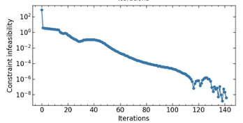
3.1 Inverted Pendulum
Here we consider the problem of stabilizing an inverted pendulum. The dynamics of the pendulum is as follows
| (31) |
where the states are the angle and the angular velocity, is the control input. Step size and initial condition is chosen. The control inputs are bounded using inequality constraints while the terminal states are bounded using equality constraints . The initial guess for control inputs is randomly chosen from interval , and the control horizon is chosen to be . The running cost is as follows
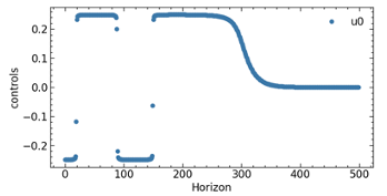
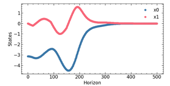
3.2 Continuous Stirred Tank Reactor
Here, we consider an example of a reactor in which a highly exothermic reaction occurs. A cooling agent maintains the reactor’s temperature at a certain value, otherwise, the temperature rapidly increases and degrades the product and/or the reactor. The following equations give the dynamics of the reactor
| (32) | ||||
where the states are the concentration of the product in the reactor, the temperature in the reactor, and the temperature of the coolant used respectively. All other constants are as follows - the activation energy J/gmol, Arrhenius constant 1/min, gas constant J/gmol/K, reactor volume liters, density g/liter, heat capacity J/g/K, enthalpy of reaction J/gmol, heat transfer coefficient J/min/K, feed flowrate liters/min, inlet feed concentration gmol/liter, inlet feed temperature K, coolant feed temperature K, coolant jacket volume liters. The coolant flowrate is the control input . The initial states are given as and the initial steady state value of coolant flowrate is .
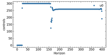
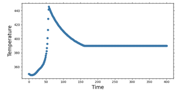
We convert the continuous-time dynamics in 32 into discrete-time using a fixed step rk45 solver. We choose a control horizon . The coolant flowrate is used to control the temperature inside the reactor to . We bound the control inputs using inequality constraints and the terminal reactor temperature using equality constraints . We use the following running cost
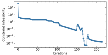
3.3 Car Parking
We also consider the car parking example from Tassa et al. (2014). The following equation gives the dynamics of the system
| (33) |
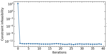
where the states are the x-coordinate, the y-coordinates, the cars heading and the velocity of the car, are the front wheel steering angle and acceleration. , , and the distance between the front and back axles of a car . The initial condition is chosen with normally distributed control inputs and control horizon of . The control inputs are bounded with inequality constraints , and the running cost and the terminal cost are as follows
where the function . The optimal solution is reached within 40 iterations of the algorithm with a solution accuracy of as shown in figure 3
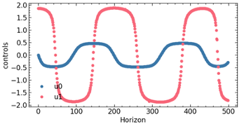
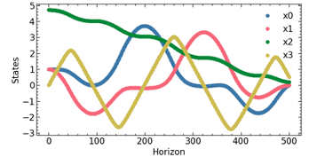
3.4 Car Obstacle
Next, we consider a 2D car with the following dynamics
| (34) |
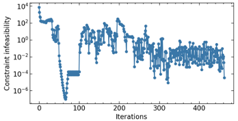
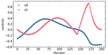
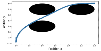
where the states and the control inputs . Given the initial conditions , the goal is to reach the terminal state using control inputs that are bounded using inequality constraints , and avoiding three obstacles defined using the following inequality constraints
The initial guess from control inputs is chosen uniformly between and a control horizon of is chosen. We observe that the algorithm successfully generates a trajectory that avoids the obstacles, as shown in figure 4
4 Conclusion
Solving DDP with arbitrary equality and inequality state and control constraints has been demonstrated. Adding slack variables to inequality constraints allows us to use an infeasible trajectory as an initial guess. Furthermore, explicit update equations for controls, lagrange variables, and slack variables have been obtained. We also apply this algorithm to a few example systems such as inverted pendulum, continuously stirred tank reactor, car parking and obstacle avoidance. We can easily extend this algorithm in an iLQR setting wherein the second-order derivatives of the dynamics are neglected. A multiple-shooting variant based on Giftthaler et al. (2017); Li et al. (2023) can also be implemented.
References
- MAYNE [1966] DAVID MAYNE. A second-order gradient method for determining optimal trajectories of non-linear discrete-time systems. International Journal of Control, 3(1):85–95, 1966. doi:10.1080/00207176608921369. URL https://doi.org/10.1080/00207176608921369.
- Li and Todorov [2004] Weiwei Li and Emanuel Todorov. Iterative linear quadratic regulator design for nonlinear biological movement systems. In International Conference on Informatics in Control, Automation and Robotics, 2004. URL https://api.semanticscholar.org/CorpusID:19300.
- Howell et al. [2019] Taylor A. Howell, Brian E. Jackson, and Zachary Manchester. Altro: A fast solver for constrained trajectory optimization. In 2019 IEEE/RSJ International Conference on Intelligent Robots and Systems (IROS), pages 7674–7679, 2019. doi:10.1109/IROS40897.2019.8967788.
- Jallet et al. [2022] Wilson Jallet, Antoine Bambade, Nicolas Mansard, and Justin Carpentier. Constrained differential dynamic programming: A primal-dual augmented lagrangian approach, 2022.
- Aoyama et al. [2020] Yuichiro Aoyama, George Boutselis, Akash Patel, and Evangelos A. Theodorou. Constrained differential dynamic programming revisited, 2020.
- Plancher et al. [2017] Brian Plancher, Zachary Manchester, and Scott Kuindersma. Constrained unscented dynamic programming. In 2017 IEEE/RSJ International Conference on Intelligent Robots and Systems (IROS), pages 5674–5680, 2017. doi:10.1109/IROS.2017.8206457.
- Xie et al. [2017] Zhaoming Xie, C. Karen Liu, and Kris Hauser. Differential dynamic programming with nonlinear constraints. In 2017 IEEE International Conference on Robotics and Automation (ICRA), pages 695–702, 2017. doi:10.1109/ICRA.2017.7989086.
- Yakowitz [1986] S. Yakowitz. The stagewise kuhn-tucker condition and differential dynamic programming. IEEE Transactions on Automatic Control, 31(1):25–30, 1986. doi:10.1109/TAC.1986.1104123.
- Murray and Yakowitz [1979] Daniel M. Murray and Sidney J. Yakowitz. Constrained differential dynamic programming and its application to multireservoir control. Water Resources Research, 15(5):1017–1027, 1979. doi:https://doi.org/10.1029/WR015i005p01017. URL https://agupubs.onlinelibrary.wiley.com/doi/abs/10.1029/WR015i005p01017.
- Chen et al. [2019] Jianyu Chen, Wei Zhan, and Masayoshi Tomizuka. Autonomous driving motion planning with constrained iterative lqr. IEEE Transactions on Intelligent Vehicles, 4(2):244–254, 2019. doi:10.1109/TIV.2019.2904385.
- Chen et al. [2017] Jianyu Chen, Wei Zhan, and Masayoshi Tomizuka. Constrained iterative lqr for on-road autonomous driving motion planning. In 2017 IEEE 20th International Conference on Intelligent Transportation Systems (ITSC), pages 1–7, 2017. doi:10.1109/ITSC.2017.8317745.
- Pavlov et al. [2021] Andrei Pavlov, Iman Shames, and Chris Manzie. Interior point differential dynamic programming. IEEE Transactions on Control Systems Technology, 29(6):2720–2727, 2021. doi:10.1109/TCST.2021.3049416.
- Frey et al. [2020] Jonathan Frey, Stefano Di Cairano, and Rien Quirynen. Active-set based inexact interior point qp solver for model predictive control. IFAC-PapersOnLine, 53(2):6522–6528, 2020. ISSN 2405-8963. doi:https://doi.org/10.1016/j.ifacol.2020.12.067. URL https://www.sciencedirect.com/science/article/pii/S2405896320303232. 21st IFAC World Congress.
- Tassa et al. [2012] Yuval Tassa, Tom Erez, and Emanuel Todorov. Synthesis and stabilization of complex behaviors through online trajectory optimization. In 2012 IEEE/RSJ International Conference on Intelligent Robots and Systems, pages 4906–4913, 2012. doi:10.1109/IROS.2012.6386025.
- Wächter and Biegler [2006] Andreas Wächter and Lorenz T. Biegler. On the implementation of an interior-point filter line-search algorithm for large-scale nonlinear programming. Mathematical Programming, 106:25–57, 2006. URL https://api.semanticscholar.org/CorpusID:14183894.
- Nocedal [1997] Jorge Nocedal. On the local behavior of an interior point method for nonlinear programming. 1997. URL https://api.semanticscholar.org/CorpusID:18330431.
- Tassa et al. [2014] Yuval Tassa, Nicolas Mansard, and Emo Todorov. Control-limited differential dynamic programming. In 2014 IEEE International Conference on Robotics and Automation (ICRA), pages 1168–1175, 2014. doi:10.1109/ICRA.2014.6907001.
- Giftthaler et al. [2017] Markus Giftthaler, Michael Neunert, M. Stäuble, Jonas Buchli, and Moritz Diehl. A family of iterative gauss-newton shooting methods for nonlinear optimal control. 2018 IEEE/RSJ International Conference on Intelligent Robots and Systems (IROS), pages 1–9, 2017. URL https://api.semanticscholar.org/CorpusID:32336981.
- Li et al. [2023] He Li, Wenhao Yu, Tingnan Zhang, and Patrick M. Wensing. A unified perspective on multiple shooting in differential dynamic programming, 2023. URL https://arxiv.org/abs/2309.07872.