Quasiperiodic Floquet-Gibbs states in Rydberg atomic systems
Abstract
Open systems that are weakly coupled to a thermal environment and driven by fast, periodically oscillating fields are commonly assumed to approach an equilibrium-like steady state with respect to a truncated Floquet-Magnus Hamiltonian. Using a general argument based on Fermi’s golden rule, we show that such Floquet-Gibbs states emerge naturally in periodically modulated Rydberg atomic systems, whose lab-frame Hamiltonian is a quasiperiodic function of time. Our approach applies as long as the inherent Bohr frequencies of the system, the modulation frequency and the frequency of the driving laser, which is necessary to uphold high-lying Rydberg excitations, are well separated. To corroborate our analytical results, we analyze a realistic model of up to five interacting Rydberg atoms with periodically changing detuning. We demonstrate numerically that the second-order Floquet-Gibbs state of this system is essentially indistinguishable from the steady state of the corresponding Redfield equation if the modulation and driving frequencies are sufficiently large.
Open quantum systems in weak contact with a thermal environment generically equilibrate to a Gibbs state [1, 2, 3, 4, 5, 6, 7]
| (1) |
Since the partition function is determined by the normalization condition , this state depends only on the Hamiltonian of the system and the inverse temperature of the environment. The structure of the system-environment coupling and any dynamical properties of the environment, however, are irrelevant. Once the system is driven away from equilibrium, such a universal characterization of its state is no longer possible in general [8, 9]. A rare exception emerges when thermalization is prevented by periodically oscillating fields. The Floquet theorem [10] then guarantees that the stroboscopic dynamics of the isolated system is described by a time-independent effective Hamiltonian [11, 12, 13, 14, 15]. It thus appears plausible that the system should, at stroboscopic times, settle to a Floquet-Gibbs state of the form
| (2) |
when weakly coupled to a thermal environment [12, 16, 17, 18, 19, 20]. Two objections are commonly raised against this idea [21, 22, 23, 24]. First, the Floquet Hamiltonian is not unique, since each of its eigenvalues can be arbitrarily shifted by an integer multiple of , where is the driving frequency [25, 26, 27]. Second, can usually not be expressed as a sum of local densities, which is a necessary condition for the system to approach a Gibbs-type state [28, 29, 30, 31, 32, 33]. Both of these problems can be overcome in the high-frequency regime, where the Floquet Hamiltonian can be approximated by a truncation of an asymptotic series, which is known as Floquet-Magnus expansion [21, 34, 35]. This approach fixes eigenvalues of the Floquet Hamiltonian and introduces only a limited degree of non-locality, provided that the original Hamiltonian of the driven system features only short-range interactions and that the truncation order can be chosen sufficiently small [36]. Indeed, it has been shown that, under certain technical conditions, truncated Floquet-Gibbs state of the form
| (3) |
can, on long intermediate time scales, accurately describe open quantum systems subject to high-frequency periodic driving [36, 37]; similar conclusions can also be drawn for classical systems, although the Floquet theorem has no strict counterpart for non-linear dynamics [38, 39]. This phenomenon, which is known as Floquet prethermalization [40, 41, 41, 42, 43, 44, 45, 46, 47, 48, 49, 50], underpins the idea of Floquet engineering, which aims to create unconventional states of matter by tailoring the effective Hamiltonian of many-body systems with oscillating control fields [14, 51, 52, 53, 54, 55, 56, 57, 58].
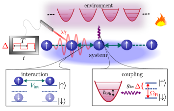
In principle, Rydberg atomic settings offer an excellent platform to apply and test this concept in practice, due to their versatility and high degree of controllability [59, 60, 61, 62, 63, 64, 65, 66, 67, 68, 69]. Such systems are shaped by fast oscillating laser fields with frequency , which are required to generate the high-lying excitations that define Rydberg atoms [70, 71, 72, 15, 73, 74]. However, this specific type of driving can usually be eliminated from the system Hamiltonian exactly by means of a local unitary transformation, as is the case for settings, where environmental effects can be neglected [75, 76]. Since is generally large on any other relevant time scale of the setup, the system thus typically attains a simple Gibbs state in the rotating frame of the driving laser [20]. To investigate the emergence of more general Floquet-Gibbs states with Rydberg atoms, it is therefore necessary to introduce an additional periodic modulation with frequency , see Fig. 1. The situation then becomes more complicated as the system Hamiltonian is now quasiperiodic function of time. It is thus no longer clear how a truncated Floquet-Gibbs state can be constructed and whether or not it still provides an adequate description of the system on some relevant time scale.
The present article seeks to address this problem. As noted above, the laser-induced time dependence of the system Hamiltonian can typically be removed by a local unitary transformation , where each acts only on a single atom and has no other eigenvalues than and so that . In the resulting rotating frame, the joint Hamiltonian of the system and its environment, usually a thermal radiation field, has the general form
| (4) |
In this expression, and are the transformed system and interaction Hamiltonians, is a small dimensionless coupling parameter and is the Hamiltonian of the environment. Thus, a strictly periodic system Hamiltonian is recovered, but the system-environment coupling now oscillates with the frequency of the laser. However, as we show next, this effect is insignificant as long as all relevant time scales are strongly separated. Specifically, we require that
| (5) |
where is the typical scale of the Bohr frequencies of the average Hamiltonian . If these conditions are satisfied, there exists an extended prethermal regime, where the truncated Floquet-Gibbs state (3) accurately describes the stroboscopic state of the driven system in the rotating frame. This result constitutes our first main insight and can be understood from the following argument.
The Floquet-Magnus expansion makes it possible to construct a time-periodic unitary transformation so that for any integer and
| (6) |
where the truncated Floquet Hamiltonian is time independent [21]. Upon using this transformation to switch to a double-rotating frame, the joint system-environment Hamiltonian (4) becomes
| (7) |
with . Since the system Hamiltonian is now time-independent, the problem can, assuming that higher-order corrections in are insignificant, be treated with standard methods of time-dependent perturbation theory, where plays the role of an expansion parameter [77, 78, 79]. We denote by and the eigenvalues of and and by and the corresponding eigenstates. In lowest order with respect to , the transition rates between the unperturbed states of the joint system are given by Fermi’s golden rule,
| (8) | ||||
where is the time evolution operator of the joint system in the double-rotating frame. Furthermore, and are the Bohr frequencies of the truncated Floquet Hamiltonian and the reservoir Hamiltonian, respectively. The sum in Eq. (8) runs over all integers and and the coefficients
| (9) | |||
result from a double Fourier expansion of the interaction matrix element. It now remains to identify the dominant contributions to the transition rates (8).
To this end, we note that , since and any higher-order terms in the Floquet-Magnus expansion are parametrically suppressed with inverse powers of . It is further plausible to assume that whenever is significant, since any natural interaction Hamiltonian should generate environment excitations of the same order of magnitude as the system energy in single-photon processes. Thus, for , the resonance condition
| (10) |
can only be met if . Since, by the Riemann-Lebesgue lemma, the coefficients decay at least as for sufficiently large , any such contributions will be subdominant in the sum (8). For , however, the condition (10) can only be satisfied if . Hence, up to sub-dominant corrections, the transition rates between the unperturbed states of the joint system are
| (11) |
Upon assuming that the environment is initially in thermal equilibrium at the inverse temperature , the transition rates between the free states of the system proper then become
| (12) |
where denotes the density of states of the environment. It is now readily verified that these rates satisfy the detailed balance condition
| (13) |
with respect to the quasi-energies and , i.e., the eigenvalues of the truncated Floquet Hamiltonian . As a result, the system relaxes to a truncated Floquet-Gibbs state of the form (3) in the double-rotating frame, as long as the conditions (5) are met. In the lab frame, the system thus approaches the quasiperiodic state
| (14) |
which provides a valid description at any time and is characterized by vanishing net energy absorption. This state can further be expected to be stable on an intermediate but practically long time scale, before heating, induced by subdominant corrections to the transition rates, prevails and a trivial infinite temperature state is attained [80, 81, 82, 83, 84].
Being reliant on qualitative arguments, the above derivation calls for further confirmation. To this end, we consider a generic many-body system of Rydberg atoms on a one-dimensional lattice, see Fig. 1. Each atom is described as a two-level system with eigenstates and , for each site , and level splitting . Transitions between the ground and excited states of the individual atoms are driven by an external laser with frequency . In the corresponding rotating frame, which is induced by the local unitary transformation , the system Hamiltonian becomes
| (15) |
with , and throughout. Furthermore, is the detuning of the laser and the Rabi frequency, which characterizes the coupling strength between laser and atoms. The last term, , describes interactions between excited Rydberg atoms, which arise from dipole-dipole or van der Waals forces [86, 71, 60, 87]. For simplicity, we assume these forces to be short-ranged so that they can be modelled with a nearest-neighbor interaction Hamiltonian of the form
| (16) |
where the parameter sets the interaction strength. The environment of the system is formed by a thermal radiation field with bare Hamiltonian
| (17) |
where the Fock-space operators and create and annihilate photons with momentum and polarization and denotes the frequency of the corresponding field mode, with being the speed of light. In the rotating frame of the laser, the general form of the full system-environment Hamiltonian is given by Eq. (4). For our model, the system-environment coupling now takes the specific form
| (18) |
where and h.c stands for Hermitian conjugate. The coupling constants are determined by the atomic dipole moment and the polarization vector of the corresponding field mode; is the dielectric constant of the vacuum and the quantization volume [88, 89].
With these prerequisites, we are ready to explore the accuracy of the approximations that lead to the quasiperiodic Floquet-Gibbs state (14). To introduce a periodic modulation, we assume that the detuning switches between and some fixed value at the frequency . That is, we choose the protocol
| (19) |
where and . Such a protocol can be realized, for instance, by controlling the level splitting of the individual atoms with external magnetic fields. The Floquet Hamiltonian can now be calculated perturbatively through the Floquet-Magnus expansion. The second-order order truncation of this series, which we use throughout this study, is given by with
| (20a) | ||||
| (20b) | ||||
| (20c) | ||||
and . As a benchmark for the corresponding quasiperiodic Floquet-Gibbs state , we use the solution of the Redfield equation [90], which follows from the microscopic model outlined above by tracing out the environmental degrees of freedom and applying the standard Born and Markov approximations. These approximations are well justified in the present setting, since the dipole-coupling between atoms and electromagnetic field modes tends to be weak and the thermal radiation field features very short correlation times. The Redfield equation, which is given by
| (21) |
in the rotating frame of the laser, can therefore be expected to describe our system’s actual dynamics accurately [91, 92, 93, 94, 95, 96]. Here, denotes the evolving density matrix of the system and the time-dependent operators and are given by
| (22) | ||||
| (23) |
where denotes the time evolution operator of the free system in the rotating frame of the laser, and the bath correlation function is given by
| (24) |
with the Bose-Einstein factors , for details, see Ref. [85].
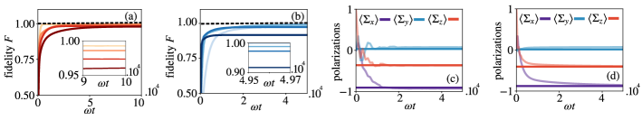
For moderate system size , the Redfield equation (21) can be solved numerically as we explain in Ref. [85]. In Fig. 2(a-d), we compare this solution with the second-order quasiperiodic Gibbs state (14) for representative parameter values. To this end, we calculate the fidelity , where . This quantity, which is defined as [97]
| (25) |
provides a measure for the similarity of two general states and and takes its maximum value if and only if . In addition, we evaluate the expectation values of the three collective polarizations
| (26) |
where and are the usual Pauli matrices in the basis spanned by the ground and excited states of the individual atoms. Our numerical results demonstrate that the system, as described by the Redfield equation (21), rapidly approaches a stroboscopic steady state, which is almost indistinguishable from the second-order Floquet-Gibbs state , as long as the inherent frequency scale of the system, the frequency of the periodic modulation and the frequency of the driving laser are separated by at least one order of magnitude. As the separation of time scales is weakened by increasing , subdominant contributions to the transition rates (8) start to play a significant role and deviations between the steady state and the Floquet-Gibbs state become more pronounced. We further note that the transient period, during which the system approaches its steady state, appears to increase monotonically with the system size , at least for the factorized initial state used in Fig. 2. This observation is plausible, since, as the system grows, more and more time will typically be required to build up the long-range correlations encoded in the Floquet-Magnus Hamiltonian; specifically, these correlations are described by the three- and four-body terms that arise from the nested commutators in Eqs. (20b) and (20c).
In summary, our case study provides ample evidence that periodically modulated Rydberg systems in weak contact with a thermal environment relax to a stable quasiperiodic Floquet-Gibbs state, as long as the three relevant time scales of system, modulation and driving are well separated. Notably, this state is stabilized by a strong detuning between the drive and the system-environment coupling, rather than a balance between energy absorption and dissipation, as one might have a priori expected. The former mechanism leads to vanishing net energy uptake as it effectively insulates the driven system from its environment, once the quasiperiodic state is reached. During the transient phase, where the quasiperiodic Floquet-Gibbs state is approached, dissipation is incurred and this process can be described quantitatively with a Lindblad-type master equation, which can be derived from the Redfield equation (21) along the same lines that lead to the detailed balance relation (13) [98, 99]. In the double-rotating frame, this equation takes the form
| (27) |
where both the Lamb shift , which commutes with the truncated Floquet-Magnus Hamiltonian , and the dissipation super operator are time-independent; the latter has Lindblad form and satisfies the quantum detailed-balance relation
| (28) |
where denotes the adjoint of with respect to the Hilbert-Schmidt scalar product and is a placeholder for an arbitrary operator, for details see Ref. [85].
The general arguments developed in the first part of this article suggest that the behavior seen in our model may in fact be indicative of a more generic phenomenology, which is likely to govern a whole variety of quasiperiodically driven systems in the high-frequency regime. We stress that these insights go beyond earlier works, which, to the best of our knowledge, have focused solely on strictly periodic driving. Along with experimental tests of our predictions, we leave it to future research to put our theory on rigorous mathematical grounds and to determine its precise range of validity and wider implications [100]. Interesting conceptual directions would be, for example, to characterize the mechanism by which the quasiperiodic state decays once the driving and modulation frequencies fall below certain thresholds or to consider the strong-coupling regime, where Fermi’s golden rule no longer applies. On the more practical side, further exploring how Rydberg atomic systems may be used to realize unconventional states of matter or how quasiperiodic driving can be deployed in quantum thermodynamics to engineer new types of thermal machines provide compelling topics for further investigations [101, 102, 103].
Data access statement: The numerical data supporting the findings of this article and the code used to generate them are available on Zenodo [104].
Acknowledgements.
Acknowledgments: We acknowledge funding from the Deutsche Forschungsgemeinschaft (DFG, German Research Foundation) through the Research Unit FOR 5413/1, Grant No. 465199066. This project has also received funding from the European Union’s Horizon Europe research and innovation program under Grant Agreement No. 101046968 (BRISQ). F.C. is indebted to the Baden-Württemberg Stiftung for the financial support by the Eliteprogramme for Postdocs. This work was supported by the University of Nottingham and the University of Tübingen’s funding as part of the Excellence Strategy of the German Federal and State Governments, in close collaboration with the University of Nottingham. This work was supported by the Medical Research Council (Grants No. MR/S034714/1 and MR/Y003845/1) and the Engineering and Physical Sciences Research Council (Grant No. EP/V031201/1).References
- Callen [1985] H. B. Callen, Thermodynamics and an introduction to thermostatistics; 2nd ed. (Wiley, New York, NY, 1985).
- Isar et al. [1994] A. Isar, A. Sandulescu, H. Scutaru, E. Stefanescu, and W. Scheid, Open quantum systems, Int. J. Mod. Phys E 3, 635 (1994).
- Carmichael [1999] H. Carmichael, Statistical Methods in Quantum Optics 1: Master Equations and Fokker-Planck Equations, Physics and Astronomy Online Library (Springer, 1999).
- Breuer and Petruccione [2002] H. Breuer and F. Petruccione, The Theory of Open Quantum Systems (Oxford University Press, 2002).
- Accardi and Imafuku [2004] L. Accardi and K. Imafuku, Dynamical detailed balance and local kms condition for non-equilibrium states, Int. J. Mod. Phys. A 18, 435 (2004).
- Rivas and Huelga [2012] A. Rivas and S. F. Huelga, Open Quantum Systems: An Introduction (Springer Berlin Heidelberg, 2012).
- Kosloff [2013] R. Kosloff, Quantum thermodynamics: A dynamical viewpoint, Entropy 15, 2100 (2013).
- Zwanzig [2001] R. Zwanzig, Nonequilibrium statistical mechanics (Oxford university press, 2001).
- Mazenko [2006] G. Mazenko, Nonequilibrium statistical mechanics (John Wiley & Sons, 2006).
- Floquet [1883] G. Floquet, Sur les équations différentielles linéaires à coefficients périodiques, in Annales scientifiques de l’École normale supérieure, Vol. 12 (1883) pp. 47–88.
- Sambe [1973] H. Sambe, Steady states and quasienergies of a quantum-mechanical system in an oscillating field, Phys. Rev. A 7, 2203 (1973).
- Torres and Kunold [2005] M. Torres and A. Kunold, Kubo formula for Floquet states and photoconductivity oscillations in a two-dimensional electron gas, Phys. Rev. B 71, 115313 (2005).
- Kitagawa et al. [2011] T. Kitagawa, T. Oka, A. Brataas, L. Fu, and E. Demler, Transport properties of nonequilibrium systems under the application of light: Photoinduced quantum hall insulators without Landau levels, Phys. Rev. B 84, 235108 (2011).
- Bukov et al. [2015] M. Bukov, L. D'Alessio, and A. Polkovnikov, Universal high-frequency behavior of periodically driven systems: from dynamical stabilization to Floquet engineering, Adv. Phys. 64, 139 (2015).
- Eckardt [2017] A. Eckardt, Colloquium: Atomic quantum gases in periodically driven optical lattices, Rev. Mod. Phys. 89, 011004 (2017).
- Shirai et al. [2015] T. Shirai, T. Mori, and S. Miyashita, Condition for emergence of the Floquet-Gibbs state in periodically driven open systems, Phys. Rev. E 91, 030101 (2015).
- Dai et al. [2016] C. M. Dai, Z. C. Shi, and X. X. Yi, Floquet theorem with open systems and its applications, Phys. Rev. A 93, 032121 (2016).
- Shirai et al. [2018] T. Shirai, T. Mori, and S. Miyashita, Floquet–Gibbs state in open quantum systems, EPJ-Special Topics 227, 323–333 (2018).
- Sato et al. [2020] S. A. Sato, U. D. Giovannini, S. Aeschlimann, I. Gierz, H. Hübener, and A. Rubio, Floquet states in dissipative open quantum systems, J. Phys. B 53, 225601 (2020).
- Mori [2023] T. Mori, Floquet states in open quantum systems, Annu. Rev. Condens. Matter Phys 14, 35 (2023).
- Blanes et al. [2009] S. Blanes, F. Casas, J. Oteo, and J. Ros, The Magnus expansion and some of its applications, Phys. Rep. 470, 151–238 (2009).
- D’Alessio and Rigol [2014] L. D’Alessio and M. Rigol, Long-time behavior of isolated periodically driven interacting lattice systems, Phys. Rev. X 4, 041048 (2014).
- Mananga and Charpentier [2016] E. S. Mananga and T. Charpentier, On the Floquet–Magnus expansion: Applications in solid-state nuclear magnetic resonance and physics, Phys. Rep. 609, 1 (2016).
- Kuwahara et al. [2016a] T. Kuwahara, T. Mori, and K. Saito, Floquet–Magnus theory and generic transient dynamics in periodically driven many-body quantum systems, Ann. Phys. 367, 96–124 (2016a).
- Grifoni and Hänggi [1998] M. Grifoni and P. Hänggi, Driven quantum tunneling, Phys. Rep. 304, 229 (1998).
- Timberlake and Reichl [1999] T. Timberlake and L. E. Reichl, Changes in Floquet-state structure at avoided crossings: Delocalization and harmonic generation, Phys. Rev. A 59, 2886 (1999).
- Kohn [2001] W. Kohn, Periodic thermodynamics, J. Stat. Phys 103, 417 (2001).
- Srednicki [1994] M. Srednicki, Chaos and quantum thermalization, Phys. Rev, E 50, 888 (1994).
- Yukalov [2011] V. Yukalov, Equilibration and thermalization in finite quantum systems, Laser Phys. Lett. 8, 485 (2011).
- Gogolin and Eisert [2016] C. Gogolin and J. Eisert, Equilibration, thermalisation, and the emergence of statistical mechanics in closed quantum systems, Rep. Prog. Phys. 79, 056001 (2016).
- D’Alessio et al. [2016] L. D’Alessio, Y. Kafri, A. Polkovnikov, and M. Rigol, From quantum chaos and eigenstate thermalization to statistical mechanics and thermodynamics, Adv. Phys. 65, 239–362 (2016).
- Farrelly et al. [2017] T. Farrelly, F. G. Brandão, and M. Cramer, Thermalization and return to equilibrium on finite quantum lattice systems, Phys. Rev. Lett. 118, 140601 (2017).
- Mori et al. [2018] T. Mori, T. N. Ikeda, E. Kaminishi, and M. Ueda, Thermalization and prethermalization in isolated quantum systems: A theoretical overview, J. Phys. B 51, 112001 (2018).
- Mananga and Charpentier [2015] E. S. Mananga and T. Charpentier, Floquet–Magnus expansion for general n-coupled spins systems in magic-angle spinning nuclear magnetic resonance spectra, Chem. Phys. 450, 83 (2015).
- Mori [2015] T. Mori, Floquet resonant states and validity of the Floquet-Magnus expansion in the periodically driven friedrichs models, Phys. Rev. A 91, 020101 (2015).
- Kuwahara et al. [2016b] T. Kuwahara, T. Mori, and K. Saito, Floquet–Magnus theory and generic transient dynamics in periodically driven many-body quantum systems, Ann. Phys. 367, 96 (2016b).
- Shirai et al. [2016] T. Shirai, J. Thingna, T. Mori, S. Denisov, P. Hänggi, and S. Miyashita, Effective Floquet–Gibbs states for dissipative quantum systems, New J. Phys. 18, 053008 (2016).
- Veness and Brandner [2023a] T. Veness and K. Brandner, Reservoir-induced stabilization of a periodically driven classical spin chain: Local versus global relaxation, Phys. Rev. E 108, 044147 (2023a).
- Veness and Brandner [2023b] T. Veness and K. Brandner, Reservoir-induced stabilization of a periodically driven many-body system, Phys. Rev. E 108, L042102 (2023b).
- Lazarides et al. [2014] A. Lazarides, A. Das, and R. Moessner, Equilibrium states of generic quantum systems subject to periodic driving, Phys. Rev. E 90, 012110 (2014).
- Weidinger and Knap [2017] S. A. Weidinger and M. Knap, Floquet prethermalization and regimes of heating in a periodically driven, interacting quantum system, Sc. Reports 7, 10.1038/srep45382 (2017).
- Mori [2018] T. Mori, Floquet prethermalization in periodically driven classical spin systems, Phys. Rev. B 98, 104303 (2018).
- Herrmann et al. [2018] A. Herrmann, Y. Murakami, M. Eckstein, and P. Werner, Floquet prethermalization in the resonantly driven Hubbard model, EPL 120, 57001 (2018).
- Rubio-Abadal et al. [2020] A. Rubio-Abadal, M. Ippoliti, S. Hollerith, D. Wei, J. Rui, S. Sondhi, V. Khemani, C. Gross, and I. Bloch, Floquet prethermalization in a Bose-Hubbard system, Phys. Rev. X 10, 021044 (2020).
- Peng et al. [2021] P. Peng, C. Yin, X. Huang, C. Ramanathan, and P. Cappellaro, Floquet prethermalization in dipolar spin chains, Nature Phys. 17, 444 (2021).
- Dalla Torre and Dentelski [2021] E. Dalla Torre and D. Dentelski, Statistical Floquet prethermalization of the Bose-Hubbard model, SciPost Phys. 11, 040 (2021).
- Beatrez et al. [2021] W. Beatrez, O. Janes, A. Akkiraju, A. Pillai, A. Oddo, P. Reshetikhin, E. Druga, M. McAllister, M. Elo, B. Gilbert, et al., Floquet prethermalization with lifetime exceeding 90s in a bulk hyperpolarized solid, Phys. Rev. Lett. 127, 170603 (2021).
- Naji et al. [2022] J. Naji, R. Jafari, L. Zhou, and A. Langari, Engineering Floquet dynamical quantum phase transitions, Phys. Rev. B 106, 094314 (2022).
- Ho et al. [2023] W. W. Ho, T. Mori, D. A. Abanin, and E. G. Dalla Torre, Quantum and classical Floquet prethermalization, Ann. Phys. 454, 169297 (2023).
- He et al. [2023] G. He, B. Ye, R. Gong, Z. Liu, K. W. Murch, N. Y. Yao, and C. Zu, Quasi-Floquet prethermalization in a disordered dipolar spin ensemble in diamond, Phys. Rev. Lett. 131, 130401 (2023).
- Kennes et al. [2018] D. Kennes, A. De La Torre, A. Ron, D. Hsieh, and A. Millis, Floquet engineering in quantum chains, Phys. Rev. Lett. 120, 127601 (2018).
- Claeys et al. [2019] P. W. Claeys, M. Pandey, D. Sels, and A. Polkovnikov, Floquet-engineering counterdiabatic protocols in quantum many-body systems, Phys. Rev. Lett. 123, 090602 (2019).
- Oka and Kitamura [2019] T. Oka and S. Kitamura, Floquet engineering of quantum materials, Annu. Rev. Condens. Matter Phys 10, 387 (2019).
- Rodriguez-Vega et al. [2021] M. Rodriguez-Vega, M. Vogl, and G. A. Fiete, Low-frequency and moiré–Floquet engineering: A review, Ann. Phys. 435, 168434 (2021).
- Weitenberg and Simonet [2021] C. Weitenberg and J. Simonet, Tailoring quantum gases by Floquet engineering, Nature Phys. 17, 1342 (2021).
- Haldar and Das [2022] A. Haldar and A. Das, Statistical mechanics of Floquet quantum matter: Exact and emergent conservation laws, J. Phys. Condens. Matter 34, 234001 (2022).
- Castro et al. [2022] A. Castro, U. De Giovannini, S. A. Sato, H. Hübener, and A. Rubio, Floquet engineering the band structure of materials with optimal control theory, Phys. Rev. Research 4, 033213 (2022).
- Lu et al. [2022] M. Lu, G. Reid, A. Fritsch, A. Piñeiro, and I. Spielman, Floquet engineering topological Dirac bands, Phys. Rev. Lett. 129, 040402 (2022).
- Gallagher [1988] T. F. Gallagher, Rydberg atoms, Rep. Prog. Phys. 51, 143 (1988).
- Saffman et al. [2010] M. Saffman, T. G. Walker, and K. Mølmer, Quantum information with Rydberg atoms, Rev. Mod. Phys. 82, 2313 (2010).
- Schmidt-Kaler et al. [2011] F. Schmidt-Kaler, T. Feldker, D. Kolbe, J. Walz, M. Müller, P. Zoller, W. Li, and I. Lesanovsky, Rydberg excitation of trapped cold ions: a detailed case study, New J. Phys. 13, 075014 (2011).
- Labuhn et al. [2016] H. Labuhn, D. Barredo, S. Ravets, S. de Léséleuc, T. Macrì, T. Lahaye, and A. Browaeys, Tunable two-dimensional arrays of single Rydberg atoms for realizing quantum ising models, Nature 534, 667 (2016).
- Marcuzzi et al. [2017] M. Marcuzzi, J. Minář, D. Barredo, S. de Léséleuc, H. Labuhn, T. Lahaye, A. Browaeys, E. Levi, and I. Lesanovsky, Facilitation dynamics and localization phenomena in Rydberg lattice gases with position disorder, Phys. Rev. Lett. 118, 063606 (2017).
- Turner et al. [2018] C. Turner, A. Michailidis, D. Abanin, M. Serbyn, and Z. Papić, Quantum scarred eigenstates in a Rydberg atom chain: Entanglement, breakdown of thermalization, and stability to perturbations, Phys. Rev. B 98, 155134 (2018).
- Lin and Motrunich [2019] C.-J. Lin and O. I. Motrunich, Exact quantum many-body scar states in the Rydberg-blockaded atom chain, Phys. Rev. Lett. 122, 173401 (2019).
- Adams et al. [2019] C. S. Adams, J. D. Pritchard, and J. P. Shaffer, Rydberg atom quantum technologies, J. Phys. B 53, 012002 (2019).
- Lin et al. [2020] C.-J. Lin, V. Calvera, and T. H. Hsieh, Quantum many-body scar states in two-dimensional Rydberg atom arrays, Phys. Rev. B 101, 220304 (2020).
- Bluvstein et al. [2021] D. Bluvstein, A. Omran, H. Levine, A. Keesling, G. Semeghini, S. Ebadi, T. T. Wang, A. A. Michailidis, N. Maskara, W. W. Ho, et al., Controlling quantum many-body dynamics in driven Rydberg atom arrays, Science 371, 1355 (2021).
- Turner et al. [2021] C. J. Turner, J.-Y. Desaules, K. Bull, and Z. Papić, Correspondence principle for many-body scars in ultracold Rydberg atoms, Phys. Rev. X 11, 021021 (2021).
- Cirac et al. [1992] J. I. Cirac, R. Blatt, P. Zoller, and W. D. Phillips, Laser cooling of trapped ions in a standing wave, Phys. Rev. A 46, 2668 (1992).
- Müller et al. [2008] M. Müller, L. Liang, I. Lesanovsky, and P. Zoller, Trapped Rydberg ions: from spin chains to fast quantum gates, New J. Phys. 10, 093009 (2008).
- Noh and Angelakis [2016] C. Noh and D. G. Angelakis, Quantum simulations and many-body physics with light, Rep. Prog. Phys. 80, 016401 (2016).
- Browaeys and Lahaye [2020] A. Browaeys and T. Lahaye, Many-body physics with individually controlled Rydberg atoms, Nat. Phys. 16, 132 (2020).
- Mallavarapu et al. [2021] S. K. Mallavarapu, A. Niranjan, W. Li, S. Wüster, and R. Nath, Population trapping in a pair of periodically driven Rydberg atoms, Phys. Rev. A 103, 023335 (2021).
- Köylüoğlu et al. [2024] N. U. Köylüoğlu, N. Maskara, J. Feldmeier, and M. D. Lukin, Floquet engineering of interactions and entanglement in periodically driven Rydberg chains (2024), arXiv:2408.02741 [quant-ph] .
- Feldmeier et al. [2024] J. Feldmeier, N. Maskara, N. U. Köylüoğlu, and M. D. Lukin, Quantum simulation of dynamical gauge theories in periodically driven Rydberg atom arrays (2024), arXiv:2408.02733 [quant-ph] .
- Merzbacher [1998] E. Merzbacher, Quantum mechanics (John Wiley & Sons, 1998).
- Messiah [2014] A. Messiah, Quantum mechanics (Courier Corporation, 2014).
- Ballentine [2014] L. E. Ballentine, Quantum mechanics: a modern development (World Scientific Publishing Company, 2014).
- Abanin et al. [2015] D. A. Abanin, W. De Roeck, and F. Huveneers, Exponentially slow heating in periodically driven many-body systems, Phys. Rev. Lett. 115, 256803 (2015).
- Reitter et al. [2017] M. Reitter, J. Näger, K. Wintersperger, C. Sträter, I. Bloch, A. Eckardt, and U. Schneider, Interaction dependent heating and atom loss in a periodically driven optical lattice, Phys. Rev. Lett. 119, 200402 (2017).
- Mallayya and Rigol [2019] K. Mallayya and M. Rigol, Heating rates in periodically driven strongly interacting quantum many-body systems, Phys. Rev. Lett. 123, 240603 (2019).
- Tran et al. [2019] M. C. Tran, A. Ehrenberg, A. Y. Guo, P. Titum, D. A. Abanin, and A. V. Gorshkov, Locality and heating in periodically driven, power-law-interacting systems, Phys. Rev. A 100, 052103 (2019).
- Mori [2022] T. Mori, Heating rates under fast periodic driving beyond linear response, Phys. Rev. Lett. 128, 050604 (2022).
- [85] See the Supplemental Material for details.
- Walker and Saffman [2008] T. G. Walker and M. Saffman, Consequences of Zeeman degeneracy for the van der Waals blockade between Rydberg atoms, Phys. Rev. A 77, 032723 (2008).
- Gambetta et al. [2019] F. M. Gambetta, I. Lesanovsky, and W. Li, Exploring nonequilibrium phases of the generalized Dicke model with a trapped Rydberg-ion quantum simulator, Phys. Rev. A 100, 022513 (2019).
- Sun and Robicheaux [2008] B. Sun and F. Robicheaux, Numerical study of two-body correlation in a 1D lattice with perfect blockade, New J. Phys. 10, 045032 (2008).
- Nill et al. [2022] C. Nill, K. Brandner, B. Olmos, F. Carollo, and I. Lesanovsky, Many-body radiative decay in strongly interacting Rydberg ensembles, Phys. Rev. Lett. 129, 243202 (2022).
- Redfield [1965] A. G. Redfield, The theory of relaxation processes, in Adv. Magn. Opt. Reson., Vol. 1 (Elsevier, 1965) pp. 1–32.
- Thingna et al. [2012] J. Thingna, J.-S. Wang, and P. Hänggi, Generalized Gibbs state with modified Redfield solution: Exact agreement up to second order, J. Chem. Phys. 136 (2012).
- Montoya-Castillo et al. [2015] A. Montoya-Castillo, T. C. Berkelbach, and D. R. Reichman, Extending the applicability of Redfield theories into highly non-Markovian regimes, J. Chem. Phys. 143 (2015).
- Hartmann and Strunz [2020] R. Hartmann and W. T. Strunz, Accuracy assessment of perturbative master equations: Embracing nonpositivity, Phys. Rev. A 101, 012103 (2020).
- Wu and Eckardt [2020] L.-N. Wu and A. Eckardt, Prethermal memory loss in interacting quantum systems coupled to thermal baths, Phys. Rev. B 101, 220302 (2020).
- Becker et al. [2021] T. Becker, L.-N. Wu, and A. Eckardt, Lindbladian approximation beyond ultraweak coupling, Phys. Rev. E 104, 014110 (2021).
- D’Abbruzzo et al. [2023] A. D’Abbruzzo, V. Cavina, and V. Giovannetti, A time-dependent regularization of the Redfield equation, SciPost Phys. 15, 117 (2023).
- Nielsen and Chuang [2010] M. A. Nielsen and I. L. Chuang, Quantum Computation and Quantum Information: 10th Anniversary Edition (Cambridge University Press, 2010).
- Davies [1974] E. B. Davies, Markovian master equations, Commun. Math. Phys. 39, 91 (1974).
- Lindblad [1976] G. Lindblad, On the generators of quantum dynamical semigroups, Commun. Math. Phys. 48, 119 (1976).
- Szczygielski [2014] K. Szczygielski, On the application of Floquet theorem in development of time-dependent Lindbladians, J. Math. Phys 55 (2014).
- Szczygielski et al. [2013] K. Szczygielski, D. Gelbwaser-Klimovsky, and R. Alicki, Markovian master equation and thermodynamics of a two-level system in a strong laser field, Phys. Rev. E 87, 012120 (2013).
- Carollo et al. [2020] F. Carollo, F. M. Gambetta, K. Brandner, J. P. Garrahan, and I. Lesanovsky, Nonequilibrium quantum many-body Rydberg atom engine, Phys. Rev. Lett. 124, 170602 (2020).
- Martins et al. [2023] W. S. Martins, F. Carollo, W. Li, K. Brandner, and I. Lesanovsky, Rydberg-ion flywheel for quantum work storage, Phys. Rev. A 108, L050201 (2023).
- Martins [2024] W. S. Martins, wsantmartins/2023-eff-floquet-gibbs-rydberg- ensembles: Quasiperiodic Floquet-Gibbs states in Rydberg atomic systems (2024).