A Unified Framework for Neural Computation and Learning Over Time

Stefano Melacci
DIISM
University of Siena, Italy
stefano.melacci@unisi.it
\AndAlessandro Betti
Scuola IMT Alti Studi Lucca
Lucca, Italy
alessandro.betti@imtlucca.it
\AndMichele Casoni
DIISM
University of Siena, Italy
m.casoni@student.unisi.it
\AndTommaso Guidi
DINFO
University of Florence, Italy
tommaso.guidi@unifi.it
\AndMatteo Tiezzi
Italian Institute of Technology
Genoa, Italy
matteo.tiezzi@iit.it
\AndMarco Gori
DIISM
University of Siena, Italy
marco.gori@unisi.it
Abstract

This paper proposes Hamiltonian Learning, a novel unified framework for learning with neural networks “over time”, i.e., from a possibly infinite stream of data, in an online manner, without having access to future information. Existing works focus on the simplified setting in which the stream has a known finite length or is segmented into smaller sequences, leveraging well-established learning strategies from statistical machine learning. In this paper, the problem of learning over time is rethought from scratch, leveraging tools from optimal control theory, which yield a unifying view of the temporal dynamics of neural computations and learning. Hamiltonian Learning is based on differential equations that: ($i$) can be integrated without the need of external software solvers; ($ii$) generalize the well-established notion of gradient-based learning in feed-forward and recurrent networks; ($iii$) open to novel perspectives. The proposed framework is showcased by experimentally proving how it can recover gradient-based learning, comparing it to out-of-the box optimizers, and describing how it is flexible enough to switch from fully-local to partially/non-local computational schemes, possibly distributed over multiple devices, and BackPropagation without storing activations. Hamiltonian Learning is easy to implement and can help researches approach in a principled and innovative manner the problem of learning over time.

1 Introduction

Motivations.   A longstanding challenge in machine learning with neural networks is the one of designing models and learning strategies that are naturally conceived to learn “over time”, progressively adapting to the information from a stream of data [1, 2]. This implies dealing with possibly infinite streams, online learning, no access to future information, thus going beyond classic statistical methods exploiting offline-collected datasets. In this paper, tools from optimal control theory [3] are exploited to rethink learning over time from scratch, proposing a unifying framework named Hamiltonian Learning (HL). Differential equations drive the learning dynamics, which are integrated going “forward” in time, i.e., without back-propagating to the past. Although related tools are widely used (in a different way) in reinforcement learning [4], and there exist works exploiting control theory in the context of neural networks [5, 6, 7], to the best of our knowledge they have not addressed the general problem of learning over time from a continuous, possibly infinite, stream of data. A few recent exceptions do exist, but they are focused on specific cases with significant limitations [8, 9]. HL is rooted on a state-space formulation of the neural model, that yields computations which are fully local in space and time. The popularity of state-space models has become prominent in recent literature [10, 11, 12], further motivating the HL perspective to create a strong connection between control theory and machine learning [13].

Contributions.   The main contributions of this paper are the following. ($i$) We propose a unified framework for neural computation and learning over time, exploiting well-established tools from optimal control theory. HL is designed to leverage the Hamilton Equations [3] to learn in a forward manner, facing an initial-value problem, instead of a boundary-value problem (Section 2–preliminaries, Section 3–HL). ($ii$) We (formally and experimentally) show that, by integrating the differential equations with the Euler method, thus without any off-the-shelf solvers for differential equations, and enforcing a sequential constraint to the update operations (which are otherwise fully parallel), our framework recovers the most popular gradient-based learning, i.e., BackPropagation and BackPropagation Through Time (Section 4). ($ii$) We discuss how HL provides a uniform and flexible view of neural computation over a stream of data, which is fully local in time and space. This favours customizability in terms of parallelization, distributed computation, and it also generalizes approaches to memory efficient BackPropagation (also Through Time) without storing outputs/activations (Section 5). The generality of HL is not intended to provide tools to solve classic issues in lifelong/continual learning (e.g., catastrophic forgetting), but to provide researches with a flexible framework that, due to its novelty, generality, and accessibility, might open to novel achievement in learning over time, which is not as mature as offline learning.

2 Preliminaries

Notation.   At time $t\geq 0$ data $\mathrm{\bf u}_{t}\in\mathbb{R}^{d}$ is provided to a neural network (for inference and learning), with learnable parameters collected into vector ${\textpdfrender{TextRenderingMode=FillStroke,LineWidth=.4pt,}{\theta}}$, with $t\in[0,N)$, $N>0$, that could be possibly $\infty$. Our framework is devised in a continuous-time setting, which, as usual, is implemented by evaluating functions at discrete time instants, that might be not evenly spaced. We avoid introducing further notation to formalize the transition from continuous-time differential equations to the outcome of the discrete-time integration steps, which will be clear from the context. Vectors are indicated in bold (they are column vectors–lowercase), where $\mathrm{\bf o}^{T}$ is the transpose of $\mathrm{\bf o}$. The notation $[\mathrm{\bf o},\mathrm{\bf u}]$ is the concatenation of the comma-separated vectors in brackets. Given an $m$-real-valued function, e.g., $r(\mathrm{\bf u})$ returning vector $\mathrm{\bf o}$, the Jacobian matrix with respect to its argument of length $d$ is a matrix in $\mathbb{R}^{m\times d}$. As a consequence, gradients of scalar functions ($m=1$) are row vectors. The only exception to this rule is in the case of derivatives with respect to time, indicated with $\dot{\mathrm{\bf o}}$, that are still column vectors, as $\mathrm{\bf o}$. We will frequently follow the convention of writing $\mathrm{\bf o}$ in place of $r(\mathrm{\bf u},{\mathrm{\bf h}})$, keeping track of the dependencies with respect to the arguments of $r$. Dependencies do not propagate through time. The operator $\odot$ is the Hadamard product.

Feed-Forward and Recurrent Networks.   A feed-forward neural model (including convolutional nets) is a (possibly deep) architecture that, given input $\mathrm{\bf u}$, computes the values of the output neurons as $\mathrm{\bf h}={f}(\mathrm{\bf u},{\textpdfrender{TextRenderingMode=FillStroke,LineWidth=.4pt,}{\theta}})$. Recurrent models are designed to process finite sequences of samples, such as $\mathrm{\bf u}_{0}$, $\mathrm{\bf u}_{1}$, $\ldots$, $\mathrm{\bf u}_{n-1}$, where we can evaluate the output values of the recurrent neurons at step $\kappa+1$ as,

$$\begin{split}\mathrm{\bf h}_{\kappa+1}&={f}(\mathrm{\bf u}_{\kappa},\mathrm{\bf h}_{\kappa},{\textpdfrender{TextRenderingMode=FillStroke,LineWidth=.4pt,}{\theta}}),\quad\text{for }\kappa=0,1,\ldots,n-1.\end{split}$$ (1)

In this case, computations depend on the initial $\mathrm{\bf h}_{0}$ which is commonly set to zeros or to random values [14]. Notice that ${\textpdfrender{TextRenderingMode=FillStroke,LineWidth=.4pt,}{\theta}}$ is not a function of $\kappa$, since the same weights are used to process the whole sequence. Moreover, Eq. 1 is a generalization of feed-forward networks, which are obtained by keeping $\kappa$ fixed and setting the second argument of $f$ to $\mathrm{\bf 0}$ (vector of zeros). Learning consists in determining the optimal value of ${\textpdfrender{TextRenderingMode=FillStroke,LineWidth=.4pt,}{\theta}}$, in the sense of minimizing a given loss function. For example, in the case of classic online gradient, weights are updated after having processed each example (feed-forward nets), or each sequence (recurrent nets). Formally, at a generic step $\upsilon$,

$${\textpdfrender{TextRenderingMode=FillStroke,LineWidth=.4pt,}{\theta}}_{\upsilon+1}={\textpdfrender{TextRenderingMode=FillStroke,LineWidth=.4pt,}{\theta}}_{\upsilon}-\gamma\tilde{{\textpdfrender{TextRenderingMode=FillStroke,LineWidth=.4pt,}{\theta}}}_{\upsilon}$$ (2)

where $\gamma>0$ is the learning rate and $-\gamma\tilde{{\textpdfrender{TextRenderingMode=FillStroke,LineWidth=.4pt,}{\theta}}}_{\upsilon}$ is the variation.

State and Stream.   In this paper we consider an extended definition of state with respect to the one used in recurrent networks, $\mathrm{\bf h}$. In particular, the state here is $[\mathrm{\bf h},\theta]$, which represents a snapshot of the model at a certain time instant, including all the information that is needed to compute Eq. 1 when an input is given. Differently from dataset-oriented approaches, here we consider a unique source of information, the stream $\mathcal{S}$, that, at time $t$, yields an input-target pair, $\mathcal{S}_{t}=(\mathrm{\bf u}_{t},\hat{\mathrm{\bf y}}_{t})$,111Targets could also be present only for some $t$’s.. We will avoid explicitly mentioning batched data, even if what we present in this paper is fine also in the case in which $\mathcal{S}$ returns mini-batches. In practice, $\mathcal{S}$ yields data only at specific time instants $t_{1},t_{2},\ldots,t_{\infty}$, which may be evenly or unevenly spaced. To keep the notation simple, we will assume a consistent spacing of $\tau$ between all consecutive samples, although our proposed method does not require evenly spaced samples (see also Appendix A).

Refer to caption
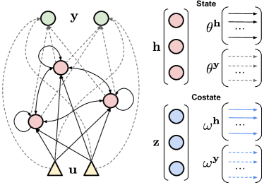
Figure 1: Left: State net (solid lines) and output net (dashed lines); Right: state ($\mathrm{\bf h}$ and ${\textpdfrender{TextRenderingMode=FillStroke,LineWidth=.4pt,}{\theta}}=[{\textpdfrender{TextRenderingMode=FillStroke,LineWidth=.4pt,}{\theta}}^{{\mathrm{\bf h}}},{\textpdfrender{TextRenderingMode=FillStroke,LineWidth=.4pt,}{\theta}}^{\mathrm{\bf y}}]$). Costate ($\mathcal{\bf z}$ and $\textpdfrender{TextRenderingMode=FillStroke,LineWidth=.4pt,}{\omega}=[\textpdfrender{TextRenderingMode=FillStroke,LineWidth=.4pt,}{\omega}^{\mathrm{\bf h}},\textpdfrender{TextRenderingMode=FillStroke,LineWidth=.4pt,}{\omega}^{\mathrm{\bf y}}]$) is also shown (not part of the net).
Init $\mathrm{\bf h}_{0}$, ${\textpdfrender{TextRenderingMode=FillStroke,LineWidth=.4pt,}{\theta}}_{0}$, $\mathcal{\bf z}_{0}$, $\textpdfrender{TextRenderingMode=FillStroke,LineWidth=.4pt,}{\omega}_{0}$, $t$. Select $\eta\geq 0$, ${\textpdfrender{TextRenderingMode=FillStroke,LineWidth=.4pt,}{\beta}}>0$, and function $\phi_{t}$.
  
while $true$ do
       
     $(\mathrm{\bf u}_{t},\hat{\mathrm{\bf y}}_{t})\leftarrow\mathcal{S}_{t}$
       
     $\dot{\mathrm{\bf h}}_{t}\hskip-1.42262pt=\hskip-1.42262ptf^{\mathrm{\bf h}}(\mathrm{\bf u}_{t},\mathrm{\bf h}_{t},\mathrm{\bf\theta}_{t}^{\mathrm{\bf h}})$ ($\mathcal{E}$ $\star$1),     $\mathrm{\bf y}_{t}\hskip-1.42262pt=\hskip-1.42262ptf^{\mathrm{\bf y}}(\mathrm{\bf u}_{t},\mathrm{\bf h}_{t},\mathrm{\bf\theta}^{\mathrm{\bf y}}_{t})$,     $\dot{\textpdfrender{TextRenderingMode=FillStroke,LineWidth=.4pt,}{\theta}}_{t}\hskip-1.42262pt=\hskip-1.42262pt-{\textpdfrender{TextRenderingMode=FillStroke,LineWidth=.4pt,}{\beta}}\odot\textpdfrender{TextRenderingMode=FillStroke,LineWidth=.4pt,}{\omega}_{t}$ ($\mathcal{E}$ $\star$2)
       
     $H^{\prime}(\mathrm{\bf h}_{t},{\textpdfrender{TextRenderingMode=FillStroke,LineWidth=.4pt,}{\theta}}_{t})=L(\mathrm{\bf y}_{t},\hat{\mathrm{\bf y}}_{t})\phi_{t}+\mathcal{\bf z}_{t}^{T}\dot{\mathrm{\bf h}}_{t}$ (9)
       
     $\dot{\mathcal{\bf z}}_{t}=\left(\frac{\partial H^{\prime}(\mathrm{\bf h}_{t},{\textpdfrender{TextRenderingMode=FillStroke,LineWidth=.4pt,}{\theta}}_{t})}{\partial\mathrm{\bf h}_{t}}\right)^{\hskip-2.84526ptT}\hskip-4.2679pt-\eta\mathcal{\bf z}_{t}$ ($\mathcal{E}$ $\star$3),     $\dot{\textpdfrender{TextRenderingMode=FillStroke,LineWidth=.4pt,}{\omega}}_{t}=\left(\frac{\partial H^{\prime}(\mathrm{\bf h}_{t},{\textpdfrender{TextRenderingMode=FillStroke,LineWidth=.4pt,}{\theta}}_{t})}{\partial{\textpdfrender{TextRenderingMode=FillStroke,LineWidth=.4pt,}{\theta}}_{t}}\right)^{\hskip-2.84526ptT}\hskip-4.2679pt-\eta\textpdfrender{TextRenderingMode=FillStroke,LineWidth=.4pt,}{\omega}_{t}$ ($\mathcal{E}$ $\star$4)
       
     ${\mathrm{\bf h}}_{t+\tau}={\mathrm{\bf h}}_{t}+\tau\dot{\mathrm{\bf h}}_{t}$,     ${\textpdfrender{TextRenderingMode=FillStroke,LineWidth=.4pt,}{\theta}}_{t+\tau}={\textpdfrender{TextRenderingMode=FillStroke,LineWidth=.4pt,}{\theta}}_{t}+\tau\dot{\textpdfrender{TextRenderingMode=FillStroke,LineWidth=.4pt,}{\theta}}_{t}$,     $\mathcal{\bf z}_{t+\tau}=\mathcal{\bf z}_{t}+\tau\dot{\mathcal{\bf z}}_{t}$,     $\textpdfrender{TextRenderingMode=FillStroke,LineWidth=.4pt,}{\omega}_{t+\tau}=\textpdfrender{TextRenderingMode=FillStroke,LineWidth=.4pt,}{\omega}_{t}+\tau\dot{\textpdfrender{TextRenderingMode=FillStroke,LineWidth=.4pt,}{\omega}}_{t}$
       
     $t=t+\tau$
       
end while

Algorithm 1 Hamiltonian Learning (what we propose is valid also for unevenly spaced data).

3 Hamiltonian Learning

Control theory is focused on finding valid configurations (controls) to optimally drive the temporal dynamics of a system. In the case of neural networks, we aim at finding the “optimal” way to drive the predictions of the model over time, by controlling the changes in ${\textpdfrender{TextRenderingMode=FillStroke,LineWidth=.4pt,}{\theta}}$. This section presents HL by introducing the main involved components one after the other, and finally describing the differential equations at the core of HL. In order to keep HL accessible to a larger audience, we skip those formal aspects that are not explicitly needed to discuss HL from an operational perspective (see Appendix B for a formal description of control theory).

State-Space Formulation.   Following the formalism of continuous-time state-space models [12], we split the computations of the network as the outcome of two sub-networks: the neuron state network, implementing function ${f}^{{\mathrm{\bf h}}}$, is responsible of computing how $\mathrm{\bf h}$ changes over time; the output network, implementing function $f^{\mathrm{\bf y}}$, is a recurrence-free portion of the network that receives data from $\mathrm{\bf h}$ and, if needed, from the input units, propagating information to the output ones, as sketched in Fig. 1. Formally,

$\displaystyle\dot{{\mathrm{\bf h}}}_{t}={f}^{{\mathrm{\bf h}}}(\mathrm{\bf u}_{t},{\mathrm{\bf h}}_{t},{\textpdfrender{TextRenderingMode=FillStroke,LineWidth=.4pt,}{\theta}}^{{\mathrm{\bf h}}}_{t})$ neuron state network (3)
$\displaystyle\vphantom{\dot{{\textpdfrender{TextRenderingMode=FillStroke,LineWidth=.4pt,}{\theta}}}}\mathrm{\bf y}_{t}=f^{\mathrm{\bf y}}(\mathrm{\bf u}_{t},{\mathrm{\bf h}}_{t},{\textpdfrender{TextRenderingMode=FillStroke,LineWidth=.4pt,}{\theta}}^{\mathrm{\bf y}}_{t})$ output network (4)
$\displaystyle\dot{{\textpdfrender{TextRenderingMode=FillStroke,LineWidth=.4pt,}{\theta}}}_{t}={\textpdfrender{TextRenderingMode=FillStroke,LineWidth=.4pt,}{\beta}}\odot\bar{{\textpdfrender{TextRenderingMode=FillStroke,LineWidth=.4pt,}{\theta}}}_{t}$ weight velocity (5)

where ${\textpdfrender{TextRenderingMode=FillStroke,LineWidth=.4pt,}{\theta}}^{{\mathrm{\bf h}}}_{t}$ and ${\textpdfrender{TextRenderingMode=FillStroke,LineWidth=.4pt,}{\theta}}^{\mathrm{\bf y}}_{t}$ are weights of the two networks, both of them function of time, with ${\textpdfrender{TextRenderingMode=FillStroke,LineWidth=.4pt,}{\theta}}_{t}=[{\textpdfrender{TextRenderingMode=FillStroke,LineWidth=.4pt,}{\theta}}^{{\mathrm{\bf h}}}_{t},{\textpdfrender{TextRenderingMode=FillStroke,LineWidth=.4pt,}{\theta}}^{\mathrm{\bf y}}_{t}]$. Eq. 5 formalizes the dynamics of the weights, that will change over time. The term ${\textpdfrender{TextRenderingMode=FillStroke,LineWidth=.4pt,}{\beta}}$ is a customizable vector of positive numbers of the same size of ${\textpdfrender{TextRenderingMode=FillStroke,LineWidth=.4pt,}{\theta}}$, that can be used to tune the relative importance of each weight (it can be written also as function of time), while $\bar{{\textpdfrender{TextRenderingMode=FillStroke,LineWidth=.4pt,}{\theta}}}$ is the unscaled weight velocity. Computing ${\mathrm{\bf h}}$ (resp. ${\textpdfrender{TextRenderingMode=FillStroke,LineWidth=.4pt,}{\theta}}$) requires us to integrate Eq. 3 (resp. Eq. 5). When using the explicit Euler’s method with step $\tau$, replacing the derivative with a forward finite difference, we get

$${\mathrm{\bf h}}_{t+\tau}={\mathrm{\bf h}}_{t}+\tau\dot{\mathrm{\bf h}}_{t},\quad\quad\quad{\textpdfrender{TextRenderingMode=FillStroke,LineWidth=.4pt,}{\theta}}_{t+\tau}={\textpdfrender{TextRenderingMode=FillStroke,LineWidth=.4pt,}{\theta}}_{t}+\tau\dot{\textpdfrender{TextRenderingMode=FillStroke,LineWidth=.4pt,}{\theta}}_{t},$$ (6)

given some ${\mathrm{\bf h}}_{0}$ and ${\textpdfrender{TextRenderingMode=FillStroke,LineWidth=.4pt,}{\theta}}_{0}$. Notice that no future information is exploited, guaranteeing a form of temporal causality, and that, at time $t$, we do not keep track of the way $\mathrm{\bf h}_{t}$ was computed, discarding dependencies from the past.

Learning Basics.   The appropriateness of the network’s predictions at $t$ is measured by a differentiable loss function $L$. It is crucial to introduce regularity on the temporal dimension, to avoid trivial solutions in which weights abruptly change from a time instant to the following one. We define cost, computed by function $C$, as a mixture of instantaneous loss $L(\mathrm{\bf y}_{t},\hat{\mathrm{\bf y}}_{t})$, and a penalty that discourages fast changes to the weights of the model,

$$C(\mathrm{\bf h}_{t},{\textpdfrender{TextRenderingMode=FillStroke,LineWidth=.4pt,}{\theta}}_{t},\bar{{\textpdfrender{TextRenderingMode=FillStroke,LineWidth=.4pt,}{\theta}}}_{t},t)=L\left(f^{\mathrm{\bf y}}(\mathrm{\bf u}_{t},{\mathrm{\bf h}}_{t},{\textpdfrender{TextRenderingMode=FillStroke,LineWidth=.4pt,}{\theta}}^{\mathrm{\bf y}}_{t}),\hat{\mathrm{\bf y}}_{t}\right)\phi_{t}+\frac{1}{2}\|\bar{{\textpdfrender{TextRenderingMode=FillStroke,LineWidth=.4pt,}{\theta}}}_{t}\|^{2},$$ (7)

where $\|\bar{{\textpdfrender{TextRenderingMode=FillStroke,LineWidth=.4pt,}{\theta}}}\|^{2}$ is the squared Euclidean norm of vector $\bar{{\textpdfrender{TextRenderingMode=FillStroke,LineWidth=.4pt,}{\theta}}}$. In Eq. 7 we also introduced a (customizable) positive scalar-valued function $\phi_{t}$ to tune the scale of the loss over time. The explicit dependence of $C$ on time is also due to the data (input-target) streamed at time $t$. If targets are not provided at time $t$, the loss $L$ is not evaluated.

Optimal Control.   The goal of learning is to minimize the total cost on the considered time horizon w.r.t. the dynamics that drive the way weights change over time, Eq. 5,

$$\bar{{\textpdfrender{TextRenderingMode=FillStroke,LineWidth=.4pt,}{\theta}}}\in\arg\min_{\underline{{\textpdfrender{TextRenderingMode=FillStroke,LineWidth=.4pt,}{\theta}}}}\int_{0}^{N}e^{\eta t}C(\mathrm{\bf h}_{t},{\textpdfrender{TextRenderingMode=FillStroke,LineWidth=.4pt,}{\theta}}_{t},\underline{{\textpdfrender{TextRenderingMode=FillStroke,LineWidth=.4pt,}{\theta}}}_{t},t)\ dt,$$ (8)

which is basically saying that we are looking for the best way to move/control the weight values over time [3]. For this reason, $\bar{{\textpdfrender{TextRenderingMode=FillStroke,LineWidth=.4pt,}{\theta}}}$ represents the optimal trajectory of the weight velocity, i.e., the optimal control of the problem. The cost is scaled by an exponential function with $\eta\geq 0$ that has no effects when $\eta=0$. As it will be clearer in the following, this choice introduces a form of dissipation, and we will show how to completely avoid computing the exponential. Control problems as Eq. 8 are boundary value problems and must be paired with initial and final conditions, which is not the case of learning over time (no knowledge of future).

Costate.   Let us introduce an adjoint variable named costate, $[\mathcal{\bf z},\textpdfrender{TextRenderingMode=FillStroke,LineWidth=.4pt,}{\omega}]$, which has the same structure/dimensions of the state $[\mathrm{\bf h},{\textpdfrender{TextRenderingMode=FillStroke,LineWidth=.4pt,}{\theta}}]$. Since ${\textpdfrender{TextRenderingMode=FillStroke,LineWidth=.4pt,}{\theta}}=[{\textpdfrender{TextRenderingMode=FillStroke,LineWidth=.4pt,}{\theta}}^{{\mathrm{\bf h}}},{\textpdfrender{TextRenderingMode=FillStroke,LineWidth=.4pt,}{\theta}}^{\mathrm{\bf y}}]$, we also have $\textpdfrender{TextRenderingMode=FillStroke,LineWidth=.4pt,}{\omega}=[\textpdfrender{TextRenderingMode=FillStroke,LineWidth=.4pt,}{\omega}^{\mathrm{\bf h}},\textpdfrender{TextRenderingMode=FillStroke,LineWidth=.4pt,}{\omega}^{\mathrm{\bf y}}]$, see Fig. 1. The costate is a largely diffused notion in the field of optimal control, following the Pontryagin’s maximum principle [3], and it has a key role in our proposal, as it will be clear shortly. In a nutshell, instead of trying to directly compute the optimal way in which the weights change over time, i.e., $\bar{{\textpdfrender{TextRenderingMode=FillStroke,LineWidth=.4pt,}{\theta}}}$ of Eq. 5 (that is a function valid $\forall t$), we will redefine the control in terms of the newly introduced costate, that will make computations maneageable in our setting. Thus, we will first estimate the costate at each $t$ and, afterwards, we will use it to evaluate $\bar{{\textpdfrender{TextRenderingMode=FillStroke,LineWidth=.4pt,}{\theta}}}$.

Hamilton Equations.   The way the costate changes over time and, more generally, the whole dynamics of the model are described by the so-called Hamilton Equations (HEs), which are the key component of HL. HEs are ODEs that provide a way of solving the problem of Eq. 8, since it can be formally shown that a minimum of Eq. 8 con be reconstructed from a solution of such ODEs [3, 15]. Since the HEs formalize how to compute $\dot{\mathrm{\bf h}}$, $\dot{\textpdfrender{TextRenderingMode=FillStroke,LineWidth=.4pt,}{\theta}}$, $\dot{\mathcal{\bf z}}$, $\dot{\textpdfrender}{TextRenderingMode=FillStroke,LineWidth=.4pt,}{\omega}$ (where the first two ones are the same as Eq. 3, Eq. 5), they also formally describe how weights change over time, i.e., $\dot{\textpdfrender{TextRenderingMode=FillStroke,LineWidth=.4pt,}{\theta}}$, which is what we need to let the network evolve. HEs are computed by differentiating the so-called Hamiltonian $H$, which is a scalar function that sums the integrand of Eq. 8 with the dot product between state $[\mathrm{\bf h},{\textpdfrender{TextRenderingMode=FillStroke,LineWidth=.4pt,}{\theta}}]$ and costate $[\mathcal{\bf z},\textpdfrender{TextRenderingMode=FillStroke,LineWidth=.4pt,}{\omega}]$. The Hamiltonian is defined in a way such that, at each $t$, it is at a minimum value with respect to the control (Appendix B). Given $H$, the HEs are $\dot{\mathrm{\bf h}}={\partial H}/{\partial\mathcal{\bf z}}$, $\dot{\textpdfrender{TextRenderingMode=FillStroke,LineWidth=.4pt,}{\theta}}={\partial H}/{\partial\textpdfrender{TextRenderingMode=FillStroke,LineWidth=.4pt,}{\omega}}$, $\dot{\mathcal{\bf z}}=-{\partial H}/{\partial\mathrm{\bf h}}$, and $\dot{\textpdfrender}{TextRenderingMode=FillStroke,LineWidth=.4pt,}{\omega}^{\mathrm{\bf h}}=-{\partial H}/{\partial{\textpdfrender{TextRenderingMode=FillStroke,LineWidth=.4pt,}{\theta}}}$ [16, 9].

Hamiltonian Learning.   In principle, the HEs at a generic time $t$ can be computed by automatic differentiation. However, HEs can only be exploited in boundary-value problems, requiring knowledge of the state at $t=0$ and of the costate at $t=N$, and then performing dynamic programming in the range $[0,N]$, updating the costate going backward in time, which is unfeasible when the dimension of the state and/or the length of the temporal interval is large. Since $T$ could be infinite, we have no ways of knowing $\mathcal{\bf z}_{N}$ or $\textpdfrender{TextRenderingMode=FillStroke,LineWidth=.4pt,}{\omega}_{N}$, and, as it is typical in online learning with causality constraints, we aim at tackling the learning problem in a forward manner, learning from the current state and current inputs, without having access to future information. Moreover, the exponentially scaled cost can introduce numerical issues for large exponents. The proposed HL framework consists of a revisited instance of the Hamiltonian and of the HEs to overcome the aforementioned issues, introducing three main features highlighted in the following with ($i$.), ($ii$.), and ($iii$.).

Forward Hamiltonian Learning.   In the HL framework, ($i$.) we avoid to deal with an exponential function of time in $H$, that leads to numerical issues, by re-parameterizing the costate in an appropriate manner, yielding an exponential-free Hamiltonian $H^{\prime}$ and exponential-free HEs (derivations in Appendix C). Moreover, ($ii$.) in the HEs, $\dot{\textpdfrender{TextRenderingMode=FillStroke,LineWidth=.4pt,}{\theta}}$ has a simple form which does not require automatic differentiation to be computed, thus we can avoid involving it in the computation of $H^{\prime}$. Putting ($i$.) and ($ii$.) together, we replace the Hamiltonian $H$ with what we refer to as Robust Hamiltonian $H^{\prime}$, which has no exponential functions of time and does not depend at all on the second part of the costate, $\dot{\textpdfrender}{TextRenderingMode=FillStroke,LineWidth=.4pt,}{\omega}$,

$$H^{\prime}(\mathrm{\bf h}_{t},{\textpdfrender{TextRenderingMode=FillStroke,LineWidth=.4pt,}{\theta}}_{t})\ =L(\mathrm{\bf y}_{t},\hat{\mathrm{\bf y}}_{t})\phi_{t}+\mathcal{\bf z}_{t}^{T}\dot{\mathrm{\bf h}}_{t}.$$ (9)

The first two HEs consist of

$\displaystyle\dot{{\mathrm{\bf h}}}_{t}$ $\displaystyle={f}^{{\mathrm{\bf h}}}(\mathrm{\bf u}_{t},{\mathrm{\bf h}}_{t},{\textpdfrender{TextRenderingMode=FillStroke,LineWidth=.4pt,}{\theta}}^{{\mathrm{\bf h}}}_{t})$ ($\mathcal{E}$ $\star$1)
$\displaystyle\dot{{\textpdfrender{TextRenderingMode=FillStroke,LineWidth=.4pt,}{\theta}}}_{t}$ $\displaystyle=-{\textpdfrender{TextRenderingMode=FillStroke,LineWidth=.4pt,}{\beta}}\odot\textpdfrender{TextRenderingMode=FillStroke,LineWidth=.4pt,}{\omega}_{t}$ ($\mathcal{E}$ $\star$2)

where Eq. $\mathcal{E}$ $\star$1 is the same as Eq. 3 (as expected), while Eq. $\mathcal{E}$ $\star$2 is what we can directly compute without involving automatic differentiation, and it involves both the parameters of the state network and the ones of the output net (since ${\textpdfrender{TextRenderingMode=FillStroke,LineWidth=.4pt,}{\theta}}$ is the concatenation of both of them). The two remaining HEs are computed by differentiating the Robust Hamiltonian,

$\displaystyle\dot{\mathcal{\bf z}}_{t}$ $\displaystyle=-s\left(\frac{\partial H^{\prime}(\mathrm{\bf h}_{t},{\textpdfrender{TextRenderingMode=FillStroke,LineWidth=.4pt,}{\theta}}_{t})}{\partial\mathrm{\bf h}_{t}}\right)^{\hskip-2.84526ptT}\hskip-4.2679pt-\eta\mathcal{\bf z}_{t}=-s\left(\phi_{t}\frac{\partial L(\mathrm{\bf y}_{t},\hat{\mathrm{\bf y}}_{t})}{\partial\mathrm{\bf h}_{t}}+\mathcal{\bf z}_{t}^{T}\frac{\partial\dot{\mathrm{\bf h}}_{t}}{\partial\mathrm{\bf h}_{t}}\right)^{\hskip-2.84526ptT}\hskip-4.2679pt-\eta\mathcal{\bf z}_{t}$ ($\mathcal{E}$ $\star$3)
$\displaystyle\dot{\textpdfrender{TextRenderingMode=FillStroke,LineWidth=.4pt,}{\omega}}_{t}$ $\displaystyle=-s\left(\frac{\partial H^{\prime}(\mathrm{\bf h}_{t},{\textpdfrender{TextRenderingMode=FillStroke,LineWidth=.4pt,}{\theta}}_{t})}{\partial{\textpdfrender{TextRenderingMode=FillStroke,LineWidth=.4pt,}{\theta}}_{t}}\right)^{\hskip-2.84526ptT}\hskip-4.2679pt-\eta\textpdfrender{TextRenderingMode=FillStroke,LineWidth=.4pt,}{\omega}_{t}=\left[\begin{aligned} \dot{\textpdfrender{TextRenderingMode=FillStroke,LineWidth=.4pt,}{\omega}}^{\mathrm{\bf h}}_{t}\vphantom{\left(\mathcal{\bf z}_{t}^{T}\frac{\partial\dot{\mathrm{\bf h}}_{t}}{\partial{\textpdfrender{TextRenderingMode=FillStroke,LineWidth=.4pt,}{\theta}}^{{\mathrm{\bf h}}}_{t}}\right)^{\hskip-2.84526ptT}}\\ \dot{\textpdfrender{TextRenderingMode=FillStroke,LineWidth=.4pt,}{\omega}}^{\mathrm{\bf y}}_{t}\vphantom{\left(\mathcal{\bf z}_{t}^{T}\frac{\partial\dot{\mathrm{\bf h}}_{t}}{\partial{\textpdfrender{TextRenderingMode=FillStroke,LineWidth=.4pt,}{\theta}}^{{\mathrm{\bf h}}}_{t}}\right)^{\hskip-2.84526ptT}}\end{aligned}\right]=\left[\begin{aligned} \vphantom{\left(\mathcal{\bf z}_{t}^{T}\frac{\partial\dot{\mathrm{\bf h}}_{t}}{\partial{\textpdfrender{TextRenderingMode=FillStroke,LineWidth=.4pt,}{\theta}}^{{\mathrm{\bf h}}}_{t}}\right)^{\hskip-2.84526ptT}}&-s\left(\mathcal{\bf z}_{t}^{T}\frac{\partial\dot{\mathrm{\bf h}}_{t}}{\partial{\textpdfrender{TextRenderingMode=FillStroke,LineWidth=.4pt,}{\theta}}^{{\mathrm{\bf h}}}_{t}}\right)^{\hskip-2.84526ptT}\hskip-4.2679pt-\eta{\textpdfrender{TextRenderingMode=FillStroke,LineWidth=.4pt,}{\omega}^{\mathrm{\bf h}}_{t}}\\ \vphantom{\left(\mathcal{\bf z}_{t}^{T}\frac{\partial\dot{\mathrm{\bf h}}_{t}}{\partial{\textpdfrender{TextRenderingMode=FillStroke,LineWidth=.4pt,}{\theta}}^{{\mathrm{\bf h}}}_{t}}\right)^{\hskip-2.84526ptT}}&-s\left(\phi_{t}\frac{\partial L(\mathrm{\bf y}_{t},\hat{\mathrm{\bf y}}_{t})}{\partial{\textpdfrender{TextRenderingMode=FillStroke,LineWidth=.4pt,}{\theta}}^{\mathrm{\bf y}}_{t}}\right)^{\hskip-2.84526ptT}\hskip-4.2679pt-\eta{\textpdfrender{TextRenderingMode=FillStroke,LineWidth=.4pt,}{\omega}^{\mathrm{\bf y}}_{t}}\end{aligned}\right],$ ($\mathcal{E}$ $\star$4)

where the additive terms weighed by $\eta$ are due to the re-parametrization that allowed us to remove the exponential function, and that act as dissipation terms, avoiding explosion of the dynamics. See Appendix C for all the derivations. In the case of Eq. $\mathcal{E}$ $\star$4, we also explicitly split the HE considering the contribution from the state networks and the one from the output network, respectively. The binary value $s\in\{-1,1\}$ does not affect the dissipation terms, and is equal to $1$ in the original HEs, which are solved backward in time. It has been recently shown how the HEs can be exploited to build models that work forward in time [15], using additional neural models to support the state-costate interaction and a time-reversed Riccati equation. Of course, the original guarantees of optimality are lost, but it opens to a viable way of learning in temporally causal manner. ($iii.$) Here we simply follow the basic intuition of reverting the direction of time when evaluating Eq. $\mathcal{E}$ $\star$3 and Eq. $\mathcal{E}$ $\star$4, and solving them going forward in time. Hence, we replace the terminal condition of the boundary-value problem with an initial one, setting the costate at time $t=0$ to zeros. Then, we force $s=-1$ in Eq. $\mathcal{E}$ $\star$3 and Eq. $\mathcal{E}$ $\star$4 to implement the aforementioned intuition about the direction of time, changing the sign of (the non-dissipative part of) the costate-related HEs. As we will show in Section 4, this choice is not only driven by intuition, but it is what allows HL to correctly generalize common gradient-based learning.

Interpretation of Hamiltonian Learning.   For each $t$, we integrate the four HEs with Euler’s method, as introduced in Eq. 6, yielding the next values of the state and costate. We do not keep track of the past states or costates, thus HEs are local in time. This requires the network to be able to keep track of the past in order to update the learnable parameters at the current time. Exactly like the state is a form of memory of what happened so far, progressively updated over time, the costate can be interpreted as a memory of the sensitivity of the model parameters. Eq. $\mathcal{E}$ $\star$3 and Eq. $\mathcal{E}$ $\star$4 shows how the dynamics of the costate involve gradients with respect to the neuron outputs and parameters at time $t$. As a consequence, when integrated, $\mathcal{\bf z}$ and $\textpdfrender{TextRenderingMode=FillStroke,LineWidth=.4pt,}{\omega}$ accumulate sensitivity information over time. We summarize HL in Algorithm 1, that is all that is needed to be implemented to setup HL, since derivatives can be computed by automatic differentiation.

Instantaneous Propagation.   When time does not bring any important information for the task at hand, e.g., as it is assumed in generic sequences instead of time-series, then we can cancel the effects of the selected integration procedure by a residual-like transition function in Eq. 3,

$\displaystyle{f}^{{\mathrm{\bf h}}}(\mathrm{\bf u}_{t},{\mathrm{\bf h}}_{t},{\textpdfrender{TextRenderingMode=FillStroke,LineWidth=.4pt,}{\theta}}^{{\mathrm{\bf h}}}_{t})$ $\displaystyle=\tau^{-1}\left(-{\mathrm{\bf h}}_{t}+{\hat{f}^{{\mathrm{\bf h}}}}(\mathrm{\bf u}_{t},{\mathrm{\bf h}}_{t},{\textpdfrender{TextRenderingMode=FillStroke,LineWidth=.4pt,}{\theta}}^{{\mathrm{\bf h}}}_{t})\right),$ (10)

where the neuron state network is basically a scaled residual network. Indeed, we add $\mathrm{\bf h}$ to the outcome of the neural computation implemented by the newly introduced function ${\hat{f}^{{\mathrm{\bf h}}}}$, and then we divide by $\tau$. In this way, when integrating the state equation (Eq. 4) with the Euler’s method, we get $\mathrm{\bf h}_{t+\tau}={\hat{f}^{{\mathrm{\bf h}}}}(\mathrm{\bf u}_{t},{\mathrm{\bf h}}_{t},{\textpdfrender{TextRenderingMode=FillStroke,LineWidth=.4pt,}{\theta}}^{{\mathrm{\bf h}}}_{t})$. In other words, the next state is what is directly computed by the neural networks, discarding time and the spacing between the streamed samples. Eq. 4 remains unchanged, since it is a static map.

4 Recovering Gradient-based Learning

HL offers a wide perspective to model learning over time with strong locality, that will be showcased in Section 5. However, in order to help trace connections with existing mainstream technologies, in this section we neglect the important locality properties of HL to clarify the relations to the usual gradient-based minimization by BackPropagation (BP) or BackPropagation Through Time (BPTT) [17]. BPTT explicitly requires to store all the intermediate states, while BP assumes instantaneous propagation of the signal through the network. First, we show how to recover gradient-based learning in feed-forward networks (BP), presenting two different ways of modeling them in HL, either by means of the output network or of the state one. Then, we do the same for recurrent networks, where, in addition to the state/output network based implementations, we also show how HL can explicitly generalize BPTT by tweaking the way data is streamed.

Feed-Forward Networks (Output Nets).   Implementing a feed-forward net by means of Eq. 4 sounds natural due to the static nature of the output map $f^{\mathrm{\bf y}}$. The notion of neuron state is lost, thus $\mathrm{\bf h}_{t}=\mathrm{\bf 0}$, $\forall t$, and, consequently $H^{\prime}$ of Eq. 9 boils down to the usual loss function. The costate-related HE of Eq. $\mathcal{E}$ $\star$4 (lower part), due to our choice of $s=-1$, is the gradient of the loss with respect to the weights (let us temporarily discard the dissipation term). When integrating the output-net-related HEs, Eq. $\mathcal{E}$ $\star$4, Eq. $\mathcal{E}$ $\star$2, respectively, setting $H^{\prime}=L$ and $s=-1$, we get

$\displaystyle\textpdfrender{TextRenderingMode=FillStroke,LineWidth=.4pt,}{\omega}^{\mathrm{\bf y}}_{t+\tau}$ $\displaystyle=\textpdfrender{TextRenderingMode=FillStroke,LineWidth=.4pt,}{\omega}^{\mathrm{\bf y}}_{t}+\tau\left(\frac{\partial L(\mathrm{\bf y}_{t},\hat{\mathrm{\bf y}}_{t})}{\partial{\textpdfrender{TextRenderingMode=FillStroke,LineWidth=.4pt,}{\theta}}^{\mathrm{\bf y}}_{t}}\phi_{t}\right)^{\hskip-2.84526ptT}\hskip-4.2679pt-\tau\eta\textpdfrender{TextRenderingMode=FillStroke,LineWidth=.4pt,}{\omega}^{\mathrm{\bf y}}_{t}=(1-\tau\eta)\textpdfrender{TextRenderingMode=FillStroke,LineWidth=.4pt,}{\omega}^{\mathrm{\bf y}}_{t}+\tau\phi_{t}\left(\frac{\partial L(\mathrm{\bf y}_{t},\hat{\mathrm{\bf y}}_{t})}{\partial{\textpdfrender{TextRenderingMode=FillStroke,LineWidth=.4pt,}{\theta}}_{t}}\right)^{\hskip-2.84526ptT}\hskip-4.2679pt$ (11)
$\displaystyle{\textpdfrender{TextRenderingMode=FillStroke,LineWidth=.4pt,}{\theta}}^{\mathrm{\bf y}}_{t+\tau}$ $\displaystyle={\textpdfrender{TextRenderingMode=FillStroke,LineWidth=.4pt,}{\theta}}^{\mathrm{\bf y}}_{t}-\tau{\textpdfrender{TextRenderingMode=FillStroke,LineWidth=.4pt,}{\beta}}^{\mathrm{\bf y}}\textpdfrender{TextRenderingMode=FillStroke,LineWidth=.4pt,}{\omega}^{\mathrm{\bf y}}_{t}.$ (12)

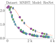
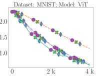
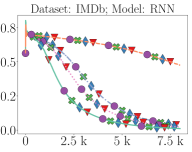
Eq. 11 is a momentum-based computation of the gradient of $L$ with respect to ${\textpdfrender{TextRenderingMode=FillStroke,LineWidth=.4pt,}{\theta}}^{\mathrm{\bf y}}$ [18], where $1-\tau\eta$ is the momentum factor and $\tau\phi_{t}$ is a time-dependent dampening coefficient. Eq. 12 is the classic weight update step, as the one we introduced in Eq. 2, with (per-parameter) learning rate $\tau{\textpdfrender{TextRenderingMode=FillStroke,LineWidth=.4pt,}{\beta}}^{\mathrm{\bf y}}$, being ${\textpdfrender{TextRenderingMode=FillStroke,LineWidth=.4pt,}{\beta}}^{\mathrm{\bf y}}$ the function ${\textpdfrender{TextRenderingMode=FillStroke,LineWidth=.4pt,}{\beta}}$ restricted to the parameters of the output network. However, in classic gradient-based learning, a specific order of operations is strictly followed: first gradient computation and, only afterwards, weights are updated with the just computed gradients. Hence, in HL we have to replace $\textpdfrender{TextRenderingMode=FillStroke,LineWidth=.4pt,}{\omega}^{\mathrm{\bf y}}_{t}$ of Eq. 12 with $\textpdfrender{TextRenderingMode=FillStroke,LineWidth=.4pt,}{\omega}^{\mathrm{\bf y}}_{t+\tau}$, and then use the definition of $\textpdfrender{TextRenderingMode=FillStroke,LineWidth=.4pt,}{\omega}^{\mathrm{\bf y}}_{t+\tau}$ given by Eq. 11. Under this constraint, we get a perfect match with classic gradient-based learning. Notice that when $\eta=1/\tau$, the momentum term disappears. In such a setting, if $\phi$ is an exponential function, it acts as an exponential scheduler of the learning rate, while if $\phi$ is constant then no scheduling is applied [19]. Of course, we can also get rid of the momentum term by zeroing the weight-costate, $\textpdfrender{TextRenderingMode=FillStroke,LineWidth=.4pt,}{\omega}^{\mathrm{\bf y}}_{t}=\mathrm{\bf 0}$ right before processing the example at time $t$. In Appendix D we report the exact rules to map learning parameters in momentum based gradient-descent and HL parameters. Fig. 2 reports the outcome of comparing gradient-based learning (with and without momentum) using popular out-of-the-box tools (different learning rates, momentum terms, damping factors and networks) and HL, showing that they lead to the same trajectories of the loss function, considering MLPs, Transformers (ViT), ResNets (see also Appendix D).

Feed-Forward Networks (State Nets).   Implementing a feed-forward network using the state network requires to clear the state $\mathrm{\bf h}_{t}$ and costate $\mathcal{\bf z}_{t}$ for each $t$, setting them to $\mathrm{\bf 0}$, to avoid propagating neuron-level information from previous examples. In this case, $f^{\mathrm{\bf y}}$ is the identity function, and we can exploit the residual-like formulation of Eq. 10 to compensate the effects of the integration procedure (that depends on $\tau$). In such a setting, we get (details in Appendix E)

$\displaystyle\mathrm{\bf h}_{t+\tau}$ $\displaystyle={\hat{f}^{{\mathrm{\bf h}}}}(\mathrm{\bf u}_{t},\mathrm{\bf h}_{t},{\textpdfrender{TextRenderingMode=FillStroke,LineWidth=.4pt,}{\theta}}^{{\mathrm{\bf h}}}_{t})=\tau\dot{\mathrm{\bf h}}_{t},$ (13)
$\displaystyle\mathcal{\bf z}_{t+\tau}^{T}$ $\displaystyle=-\tau s\phi_{t}\frac{\partial L(\mathrm{\bf h}_{t+\tau},\hat{\mathrm{\bf y}}_{t})}{\partial\mathrm{\bf h}_{t+\tau}},$ (14)

where we used $\mathrm{\bf h}_{t+\tau}$ as argument of $L$ instead of $\mathrm{\bf h}_{t}$. This choice is the direct counterpart of what we did when enforcing sequential ordering in gradient computation and weight update in the previously discussed implementation. In fact, we want the evaluation of the loss $L$ to happen after the state neurons have been updated ($\mathrm{\bf h}_{t+\tau}$), which is coherent with what happens when performing a prediction first, and only afterward evaluating the loss. Notice that, for the same reason, we also differentiate with respect to $\mathrm{\bf h}_{t+\tau}$. Eq. 13 and Eq. 14 collect the two HEs of Eq. $\mathcal{E}$ $\star$1 and Eq. $\mathcal{E}$ $\star$3, respectively. In turn, the HE of Eq. $\mathcal{E}$ $\star$4 becomes,

$$\begin{split}\dot{\textpdfrender{TextRenderingMode=FillStroke,LineWidth=.4pt,}{\omega}}^{\mathrm{\bf h}}_{t}&=-s\left(\mathcal{\bf z}_{t+\tau}^{T}\frac{\partial\dot{\mathrm{\bf h}}_{t}}{\partial{\textpdfrender{TextRenderingMode=FillStroke,LineWidth=.4pt,}{\theta}}^{{\mathrm{\bf h}}}_{t}}\right)^{\hskip-2.84526ptT}\hskip-5.69054pt-\hskip-1.42262pt\eta\textpdfrender{TextRenderingMode=FillStroke,LineWidth=.4pt,}{\omega}^{\mathrm{\bf h}}_{t}=\hskip-1.42262pt\left(\phi_{t}\frac{\partial L(\mathrm{\bf h}_{t+\tau},\hat{\mathrm{\bf y}}_{t})}{\partial\mathrm{\bf h}_{t+\tau}}\frac{\partial\mathrm{\bf h}_{t+\tau}}{\partial{\textpdfrender{TextRenderingMode=FillStroke,LineWidth=.4pt,}{\theta}}^{{\mathrm{\bf h}}}_{t}}\right)^{\hskip-2.84526ptT}-\eta\textpdfrender{TextRenderingMode=FillStroke,LineWidth=.4pt,}{\omega}^{\mathrm{\bf h}}_{t}\\ &=\left(\phi_{t}\frac{\partial L(\mathrm{\bf h}_{t+\tau},\hat{\mathrm{\bf y}}_{t})}{\partial{\textpdfrender{TextRenderingMode=FillStroke,LineWidth=.4pt,}{\theta}}^{{\mathrm{\bf h}}}_{t}}\right)^{\hskip-2.84526ptT}\hskip-4.2679pt-\eta\textpdfrender{TextRenderingMode=FillStroke,LineWidth=.4pt,}{\omega}^{\mathrm{\bf h}}_{t},\end{split}$$

where, in the first equality, we replaced $\mathcal{\bf z}_{t+\tau}$ with its definition reported in Eq. 14, while in the second one we replaced $\dot{\mathrm{\bf h}}_{t}$ with $\tau^{-1}\mathrm{\bf h}_{t+\tau}$ accordingly to Eq. 13, and discarded $s$, since $s^{2}=1$ (that is expected, since we are collapsing the dynamics of the two costate HEs). The last equality holds due to the chain rule. When integrated, it yields the same equation that we discussed in the previous implementation, Eq. 11.222Of course, replacing ${\textpdfrender{TextRenderingMode=FillStroke,LineWidth=.4pt,}{\theta}}^{\mathrm{\bf y}}$ with ${\textpdfrender{TextRenderingMode=FillStroke,LineWidth=.4pt,}{\theta}}^{{\mathrm{\bf h}}}$ and $\textpdfrender{TextRenderingMode=FillStroke,LineWidth=.4pt,}{\omega}^{\mathrm{\bf y}}$ with $\textpdfrender{TextRenderingMode=FillStroke,LineWidth=.4pt,}{\omega}^{\mathrm{\bf h}}$. Then, Eq. 12 still holds also in this case. As a consequence, all the comments we made about the analogies with momentum-based gradient learning, BP, and learning rate scheduling are valid also in this case. See Fig. 2 for comparisons with plain gradient-descent (MLP, ViT, ResNet).

Recurrent Neural Networks (Automatic Unfolding).
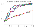
   Given a sequence of n𝑛n samples, streamed at times t0,tn1subscript𝑡0subscript𝑡𝑛1t_{0},\ldots t_{n-1}, learning in Recurrent Neural Nets (RNNs) is driven by BPTT [17], where n𝑛n states are stored while going forward, with constant weights \textpdfrenderTextRenderingMode=FillStroke,LineWidth=.4pt,θformulae-sequence\textpdfrender𝑇𝑒𝑥𝑡𝑅𝑒𝑛𝑑𝑒𝑟𝑖𝑛𝑔𝑀𝑜𝑑𝑒𝐹𝑖𝑙𝑙𝑆𝑡𝑟𝑜𝑘𝑒𝐿𝑖𝑛𝑒𝑊𝑖𝑑𝑡.4𝑝𝑡𝜃{\textpdfrender{TextRenderingMode=FillStroke,LineWidth=.4pt,}{\theta}}, and then gradients of i=0n1L(𝐲ti,𝐲^ti)superscriptsubscript𝑖0𝑛1𝐿subscript𝐲subscript𝑡𝑖subscript^𝐲subscript𝑡𝑖\sum_{i=0}^{n-1}L(\mathrm{\bf y}_{t_{i}},\hat{\mathrm{\bf y}}_{t_{i}}) with respect to \textpdfrenderTextRenderingMode=FillStroke,LineWidth=.4pt,θformulae-sequence\textpdfrender𝑇𝑒𝑥𝑡𝑅𝑒𝑛𝑑𝑒𝑟𝑖𝑛𝑔𝑀𝑜𝑑𝑒𝐹𝑖𝑙𝑙𝑆𝑡𝑟𝑜𝑘𝑒𝐿𝑖𝑛𝑒𝑊𝑖𝑑𝑡.4𝑝𝑡𝜃{\textpdfrender{TextRenderingMode=FillStroke,LineWidth=.4pt,}{\theta}} are computed in a backward manner. The most straightforward way to trace a connection between BPTT and HL is by conceiving the recurrent network in its unfolded form, and by rethinking 𝒮𝒮\mathcal{S}. If we assume 𝒮𝒮\mathcal{S} to yield one-full sequence at each time step, then we can switch our attention from the RNN to the feed-forward network obtained by unfolding it, that receives as input the whole sequence at once. Being it a feed-forward network, it can be implemented as discussed in the above text. As usual, the unfolding can be done on the fly, thus either f𝐡superscript𝑓𝐡{f}^{{\mathrm{\bf h}}} or f𝐲superscript𝑓𝐲f^{\mathrm{\bf y}} can be specifically implemented as RNNs, reusing existing software implementations. This is what we did in the Movie Review experiments (IMDb [20] data) of Fig. 2.

Recurrent Neural Networks (Hamiltonian Learning).   A more intriguing way to recover BPTT is obtained by keeping our original definition of $\mathcal{S}$, which yields a sequence streamed one-token-per-time ($n$ tokens), from $t_{0}$ to $t_{n-1}$, followed by the same tokens in reverse order (without repeating the one at time $t_{n-1}$, i.e., the sample at $t_{n-1+j}$ is equal to the one at $t_{n-1-j}$, $\forall j\geq 0$). We still exploit an identity output function and the formulation of Eq. 10 to compensate the effects of the integration. Of course we have to enforce the processing of the streamed data with the same weights, and only afterwards compute their variation, that can be achieved forcing ${\textpdfrender{TextRenderingMode=FillStroke,LineWidth=.4pt,}{\beta}}=\mathrm{\bf 0}$, $\forall t\neq 2t_{n}-t_{0}$, which is indeed a degenerate condition for ${\textpdfrender{TextRenderingMode=FillStroke,LineWidth=.4pt,}{\beta}}$ (see Eq. $\mathcal{E}$ $\star$2). When $t\leq t_{n-1}$, given some initial $\mathrm{\bf h}_{t_{0}}$, ${\textpdfrender{TextRenderingMode=FillStroke,LineWidth=.4pt,}{\theta}}_{t_{0}}$, the first two HEs, Eq. $\mathcal{E}$ $\star$1, Eq. $\mathcal{E}$ $\star$2, will drive the evolution of the system. Coherently with BPTT, we must store the sequence of the $n$ generated $\mathrm{\bf h}$’s, loosing locality. The last two HEs, Eq. $\mathcal{E}$ $\star$3, Eq. $\mathcal{E}$ $\star$4, do not bring any information, since changes in the costate will not affect ${\textpdfrender{TextRenderingMode=FillStroke,LineWidth=.4pt,}{\theta}}$, due to our choice of zeroing ${\textpdfrender{TextRenderingMode=FillStroke,LineWidth=.4pt,}{\beta}}$. When $t=t_{n_{1}}$, all the HEs play an important role, while when $t>t_{n-1}$, we basically swap the relevance of the two pairs of HEs, giving emphasis to Eq. $\mathcal{E}$ $\star$3 and Eq. $\mathcal{E}$ $\star$4, and ignoring Eq. $\mathcal{E}$ $\star$1 and Eq. $\mathcal{E}$ $\star$2, since we already stored the $n$ states. This is motivated by fact that we are going to process the reversed sequence, and we do care about tracking the sensitivity of the model with respect to changes in the learnable parameters, which is the role of the costate. The sequence of neuron states was already pre-computed, and it can be retrieved by mapping time by $\psi(t)\colon t\to 2t_{n-1}-2\tau-t$, for $t>t_{n-1}$. When integrating the costate equations, using the proposed $s=-1$, we get (details in Appendix F),

$\displaystyle\mathcal{\bf z}_{t+\tau}^{T}$ $\displaystyle=\tau\phi_{t}\frac{\partial L(\mathrm{\bf h}_{t+\tau},\hat{\mathrm{\bf y}}_{t})}{\partial\mathrm{\bf h}_{t+\tau}}+\mathcal{\bf z}_{t}^{T}\frac{\partial\mathrm{\bf h}_{t+2\tau}}{\partial\mathrm{\bf h}_{t+\tau}}-\tau\eta\mathcal{\bf z}_{t}^{T}$ (15)
$\displaystyle\textpdfrender{TextRenderingMode=FillStroke,LineWidth=.4pt,}{\omega}^{\mathrm{\bf h}}_{t+\tau}$ $\displaystyle=\textpdfrender{TextRenderingMode=FillStroke,LineWidth=.4pt,}{\omega}^{\mathrm{\bf h}}_{t}+\tau\left(\mathcal{\bf z}_{t+\tau}^{T}\frac{\partial\dot{\mathrm{\bf h}}_{t}}{\partial{\textpdfrender{TextRenderingMode=FillStroke,LineWidth=.4pt,}{\theta}}^{{\mathrm{\bf h}}}_{t}}\right)^{\hskip-2.84526ptT}\hskip-4.2679pt-\tau\eta\textpdfrender{TextRenderingMode=FillStroke,LineWidth=.4pt,}{\omega}^{\mathrm{\bf h}}_{t}$
$\displaystyle=\textpdfrender{TextRenderingMode=FillStroke,LineWidth=.4pt,}{\omega}^{\mathrm{\bf h}}_{t}+\left(\mathcal{\bf z}_{t+\tau}^{T}\frac{\partial\mathrm{\bf h}_{t+\tau}}{\partial{\textpdfrender{TextRenderingMode=FillStroke,LineWidth=.4pt,}{\theta}}^{{\mathrm{\bf h}}}_{t}}\right)^{\hskip-2.84526ptT}\hskip-4.2679pt-\tau\eta\textpdfrender{TextRenderingMode=FillStroke,LineWidth=.4pt,}{\omega}^{\mathrm{\bf h}}_{t}.$ (16)

where in the HE of Eq. $\mathcal{E}$ $\star$3, coherently with what we did for feed-forward networks, we anticipated the state-update, thus all the terms involving $\mathrm{\bf h}_{t}$ or $\dot{\mathrm{\bf h}}_{t}$ are replaced with $\mathrm{\bf h}_{t+\tau}$ and $\dot{\mathrm{\bf h}}_{t+\tau}$, respectively. In order to match BPTT, at $t=t_{n-1}$ we set the costate to $\mathrm{\bf 0}$ to clear past information (notice that while $\mathcal{\bf z}$ must be set to zeros, we can also avoid resetting $\textpdfrender{TextRenderingMode=FillStroke,LineWidth=.4pt,}{\omega}^{\mathrm{\bf h}}$, that will inherently introduce momentum, as already discussed), and we replace $t$ with $\psi_{t}-\tau$ in the time index of non-costate-related quantities, yielding

$\displaystyle\hskip-7.11317pt\mathcal{\bf z}_{t+\tau}^{T}$ $\displaystyle=\tau\phi_{{\psi_{t}-\tau}}\frac{\partial L(\mathrm{\bf h}_{\psi_{t}},\hat{\mathrm{\bf y}}_{\psi_{t}-\tau})}{\partial\mathrm{\bf h}_{\psi_{t}}}+\mathcal{\bf z}_{t}^{T}\frac{\partial\mathrm{\bf h}_{\psi_{t}+\tau}}{\partial\mathrm{\bf h}_{\psi_{t}}}-\hskip-1.42262pt\tau\eta\mathcal{\bf z}_{t}^{T}$ (17)
$\displaystyle\hskip-7.11317pt\textpdfrender{TextRenderingMode=FillStroke,LineWidth=.4pt,}{\omega}^{\mathrm{\bf h}}_{t+\tau}$ $\displaystyle=\textpdfrender{TextRenderingMode=FillStroke,LineWidth=.4pt,}{\omega}^{\mathrm{\bf h}}_{t}+\left(\mathcal{\bf z}_{t+\tau}^{T}\frac{\partial\mathrm{\bf h}_{\psi_{t}}}{\partial{\textpdfrender{TextRenderingMode=FillStroke,LineWidth=.4pt,}{\theta}}^{{\mathrm{\bf h}}}_{\psi_{t}-\tau}}\right)^{\hskip-2.84526ptT}\hskip-5.69054pt-\hskip-1.42262pt\tau\eta\textpdfrender{TextRenderingMode=FillStroke,LineWidth=.4pt,}{\omega}^{\mathrm{\bf h}}_{t}.$ (18)

When integrating the costate, the step size $\tau$ still has a role. If we select $\tau=1$ and $\eta=0$ (no dissipation), or $\phi_{t}=\tau^{-1}$ and $\eta=0$, Eq. 17 and Eq. 18 are the largely known update rules of BPTT for sequential data, as detailed in Appendix F. This correspondence has the important role of confirming the validity on the choice we made in setting $s=-1$ in HL.

Recurrent Neural Networks (Truncated).   Truncated BPTT of length $r$ can be recovered by only resetting the state at the very beginning of the input sequence and, once the end of the sequence has been reached, by streaming the last $r-1$ tokens in reverse order, going back to the previously discussed case (which implies setting neuron-costate to zero right before processing the last token of the original sequence). If $r=1$, we match the case of feed-forward neural networks, even if the initial state is not zeroed/ignored.

Refer to caption
Refer to caption
Refer to caption
Refer to caption
Refer to caption
Refer to caption
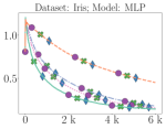
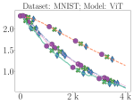
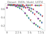
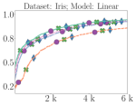
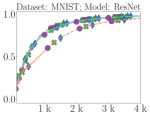
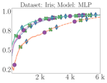
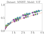
Figure 2: Comparing HL with out-of-the-box Pytorch optimizers. Each figure is about a different dataset/architecture, reporting the loss $L$ in function of time (datasets and setup in Appendix D); there are $4$ scenarios: w/o (GD-a, GD-b) and w/ momentum (Mom-a, Mom-b). In HL, we implemented each net by solely considering the output function (output), the state function (state), or, in the case of RNNs and LSTMs, jointly considering both (state/output)–the recurrent part is implemented with the state net, the rest is the output net. Curves of each scenario have the same color/linestyle, and a per-approach marker. The (absolute) difference between the weights yielded by the Pytorch optimizer and HL is zero in most cases or within the order of round-off error. Thus, curves of the same scenario overlap.

5 Leveraging Hamiltonian Learning

HL is designed to drive learning over time in stateful models in a temporally local manner. While it is general enough to recover the popular gradient-based learning in feed-forward and recurrent nets, as we discussed in Section 4, the importance of dealing with stateful networks goes beyond it. We distinguish among two use-cases where HL can be leveraged to design efficient models that learn over time.

Fully Local Learning.   The stateful nature of learning allows us to instantiate networks that are not only temporally local, but also spatially local, once we design ${f}^{{\mathrm{\bf h}}}$ to return the variations of the output values of all the its neurons. Given the graph that describes the parent/child relations among neurons, being it Directed Acyclic/Cyclic Graph, all the neurons can compute their outputs in parallel. In fact, they have the use of the full state $\mathrm{\bf h}_{t}$ (and/or the current $\mathrm{\bf u}_{t}$)–computed during the previous time step–to feed their inputs, with important connections to biologically plausible computational models and related studies [21, 22, 23]. This choice introduces delays in the computations, but it yields fully local learning, with known benefits in terms of parallelization [24] and pipeline parallelism in neural networks for multi-device computation [25] (Appendix A).

Memory Efficient BackPropagation.   The popular Neural ODEs/CDEs [5, 6] exploit a stateful model to implement the way the signal propagates through a feed-forward network [5] or when providing fixed-length sequences [6], using an ODE solver to update the state and, afterwards, to compute gradients. These models do not require to store the output of all the “layers” (which is a vague concept in Neural ODE/CDEs) while backpropagating the learning signal, since the second call to the ODE solver can basically estimate the output of the previous layer given the output of the following one. This property holds in the continuous formulation of the models, which might be prone to numerical errors when integrating on a number of discrete steps [26, 27, 28].333Costate in HL corresponds to adjoint sensitivity in Neural ODE, being them inherited from the same tools of control theory. Similarly to Neural ODE, in HL, given $\mathrm{\bf u}$ (generic input sample–we removed the time index), we can distribute the sequential computation of layers over time (see Appendix A, Eq. 20). If we integrate the state-transition with the midpoint rule [26], Eq. 6 becomes

$$\mathrm{\bf h}_{t+\tau}=\mathrm{\bf h}_{t-\tau}+\tau{{f}^{{\mathrm{\bf h}}}}(\mathrm{\bf u},\mathrm{\bf h}_{t},{\textpdfrender{TextRenderingMode=FillStroke,LineWidth=.4pt,}{\theta}}^{{\mathrm{\bf h}}}_{t}),$$ (19)

that, given $\mathrm{\bf h}_{t-\tau}$ and $\mathrm{\bf h}_{t}$ (we discard the other arguments of ${f}^{{\mathrm{\bf h}}}$ in this discussion), allows us to compute $\mathrm{\bf h}_{t+\tau}$. However, the direction of the integration can be also reversed, and the midpoint rule can also yield the previous state given the following one(s), i.e., we can compute $\mathrm{\bf h}_{t-\tau}$ given $\mathrm{\bf h}_{t}$ and $\mathrm{\bf h}_{t+\tau}$, by $\mathrm{\bf h}_{t-\tau}=\mathrm{\bf h}_{t+\tau}-\tau{{f}^{{\mathrm{\bf h}}}}(\mathrm{\bf u},\mathrm{\bf h}_{t},{\textpdfrender{TextRenderingMode=FillStroke,LineWidth=.4pt,}{\theta}}^{{\mathrm{\bf h}}}_{t})$. Notice that in both the case (direct or reversed), function ${f}^{{\mathrm{\bf h}}}$ is evaluated on the same point (differently from what would happen with Euler’s method). When using the midpoint rule, Eq. 19, HL does not have any numerical issues in re-building the output of the previous layer given the output of the following one. Moreover, we observe that two consecutive integration steps in HL, $\mathrm{\bf h}_{t+\tau}=\mathrm{\bf h}_{t-\tau}+\tau{{f}^{{\mathrm{\bf h}}}}(\mathrm{\bf u},\mathrm{\bf h}_{t},{\textpdfrender{TextRenderingMode=FillStroke,LineWidth=.4pt,}{\theta}}^{{\mathrm{\bf h}}}_{t})$ and $\mathrm{\bf h}_{t+2\tau}=\mathrm{\bf h}_{t}+\tau{{f}^{{\mathrm{\bf h}}}}(\mathrm{\bf u},\mathrm{\bf h}_{t+\tau},{\textpdfrender{TextRenderingMode=FillStroke,LineWidth=.4pt,}{\theta}}^{{\mathrm{\bf h}}}_{t+\tau})$ are exactly the equations that drive the notion of Reversible ReLU [29], once we replace $y_{1}$, $y_{2}$, $x_{1}$, $x_{2}$ of Eq. (6) in [29], with $\mathrm{\bf h}_{t+\tau}$, $\mathrm{\bf h}_{t+2\tau}$, $\mathrm{\bf h}_{t-\tau}$, $\mathrm{\bf h}_{t}$, respectively, and assuming $\mathcal{F}=\mathcal{G}={f}^{{\mathrm{\bf h}}}$, where $\mathcal{F},\mathcal{G}$ are the transition functions of Eq. (6) in [29]. Reversible ReLU allows to compute gradients without storing activations, and they are based on specifically engineered blocks. Interestingly, in HL, the same properties are simply the outcome of having changed the integration technique.

Limitations.   HL is a way to approach learning over time in a principled manner, but, of course, it does not solve the usual issues of continual learning (e.g., catastrophic forgetting [1]). Due to its forward-over-time nature, it is well-suited to deal with streams of perceptual data that does not change too abruptly. In fact, in the most local formulation of HL (Section 5), there are intrinsic delays in the propagation of information, since state and costate are updated at the same time, and weights keep changing while handing the streamed data (see Appendix A for discussions on how to trade-off locality in the computations and delays).

6 Related Work

Optimal Control.   Optimal control theory [16] provides a clear framework to handle optimization problems on a temporal horizon (Pontryagin Maximum Principle [30, 31], Dynamic Programming [32]), usually involving boundary-value problems which require iterative forward/backward schemes over the whole considered time interval or working with receding horizon control [33]. Jin et al. [34] considered the possibility of exploiting HEs for learning system dynamics and controlling policies forward-in-time, while [8] evaluated HEs in continual online learning, artificially forcing the costate dynamic to converge to zero. To our best knowledge, the relations between HEs, control theory, and gradient-based approaches were not studied from a foundational perspective in the context of learning from a stream of data with neural networks. The work of LeCun [35] mentions them, indeed, in relation with classical mechanics.

Online Learning.   There exist several works focussed on learning in an online manner from streamed data, such as in the case of physics-inspired models [36, 37] or approaches to continual online learning [38, 1]. The framework of this paper is devised by revisiting the learning problem from scratch, instead of trying to directly adapt classic statistical approaches typical of offline learning.

Neural ODE.   The methods exploited in this paper are inherited from optimal control, as it is done also in the case of Neural ODE and related works [5, 6, 27, 28, 39]. However, here we focus on the problem of learning over time in an online manner, with a possibly infinite horizon, which is different from what is commonly done in the literature of Neural ODE/CDE.

Real-Time Recurrent Learning.   The classic approach to learning online with recurrent models is RTRL [40], which requires to store, exploit, and progressively update the temporal Jacobian matrix, with high space/time complexities. Several approximations were proposed to reduce the complexity of RTRL (UORO and others, see [41]). In HL, no temporal Jacobian matrices are stored. Hence, it is not a generalization of RTRL and related work (such as Online LRU [42]).

Brain-Inspired Computing.   Neural approaches that are brain-inspired (to different extents), such as predictive coding [43, 44, 45], target propagation, local representation alignment [46, 47], forward-only learning [48, 49, 50], share the principles of locality in the computations which has been described in Section 5. HL is not inspired by brain-related dynamics but by the idea of learning over time.

7 Conclusions

We presented HL, a unified framework for neural computation and learning over time, exploiting tools from control theory. Differential equations drive learning, leveraging stateful networks that are fully local in time and space, recovering classic BackPropagation (and BPTT) in the case of non-local models. HL represents a novel perspective, that might inspire researchers to further investigate learning over time in a principled manner.

References

  • Wang et al. [2024] Liyuan Wang, Xingxing Zhang, Hang Su, and Jun Zhu. A comprehensive survey of continual learning: Theory, method and application. IEEE Transactions on Pattern Analysis and Machine Intelligence, 2024.
  • Gori and Melacci [2023] Marco Gori and Stefano Melacci. Collectionless artificial intelligence. arXiv preprint arXiv:2309.06938, 2023.
  • Bertsekas [2012] Dimitri Bertsekas. Dynamic programming and optimal control: Volume I, volume 4. Athena scientific, 2012.
  • Khetarpal et al. [2022] Khimya Khetarpal, Matthew Riemer, Irina Rish, and Doina Precup. Towards continual reinforcement learning: A review and perspectives. Journal of Artificial Intelligence Research, 75:1401–1476, 2022.
  • Chen et al. [2018] Ricky TQ Chen, Yulia Rubanova, Jesse Bettencourt, and David K Duvenaud. Neural ordinary differential equations. Advances in neural information processing systems, 31, 2018.
  • Kidger et al. [2020] Patrick Kidger, James Morrill, James Foster, and Terry Lyons. Neural controlled differential equations for irregular time series. Advances in Neural Information Processing Systems, 33:6696–6707, 2020.
  • Araujo et al. [2023] Alexandre Araujo, Aaron J Havens, Blaise Delattre, Alexandre Allauzen, and Bin Hu. A unified algebraic perspective on lipschitz neural networks. In The Eleventh International Conference on Learning Representations, 2023. URL https://openreview.net/forum?id=k71IGLC8cfc.
  • Betti et al. [2022] Alessandro Betti, Lapo Faggi, Marco Gori, Matteo Tiezzi, Simone Marullo, Enrico Meloni, and Stefano Melacci. Continual learning through hamilton equations. In Conference on Lifelong Learning Agents, pages 201–212. PMLR, 2022.
  • Betti et al. [2023] Alessandro Betti, Michele Casoni, Marco Gori, Simone Marullo, Stefano Melacci, and Matteo Tiezzi. Neural time-reversed generalized riccati equation, 2023.
  • Tiezzi et al. [2024] Matteo Tiezzi, Michele Casoni, Alessandro Betti, Tommaso Guidi, Marco Gori, and Stefano Melacci. On the resurgence of recurrent models for long sequences: Survey and research opportunities in the transformer era. arXiv preprint arXiv:2402.08132, 2024.
  • De et al. [2024] Soham De, Samuel L Smith, Anushan Fernando, Aleksandar Botev, George Cristian-Muraru, Albert Gu, Ruba Haroun, Leonard Berrada, Yutian Chen, Srivatsan Srinivasan, et al. Griffin: Mixing gated linear recurrences with local attention for efficient language models. arXiv preprint arXiv:2402.19427, 2024.
  • Gu and Dao [2023] Albert Gu and Tri Dao. Mamba: Linear-time sequence modeling with selective state spaces. arXiv preprint arXiv:2312.00752, 2023.
  • Alonso et al. [2024] Carmen Amo Alonso, Jerome Sieber, and Melanie N Zeilinger. State space models as foundation models: A control theoretic overview. arXiv preprint arXiv:2403.16899, 2024.
  • Medsker et al. [2001] Larry R Medsker, Lakhmi Jain, et al. Recurrent neural networks. Design and Applications, 5(64-67):2, 2001.
  • Betti et al. [2024] Alessandro Betti, Michele Casoni, Marco Gori, Simone Marullo, Stefano Melacci, and Matteo Tiezzi. Neural time-reversed generalized riccati equation. In Proceedings of the AAAI Conference on Artificial Intelligence, volume 38, pages 7935–7942, 2024.
  • Lewis et al. [2012] Frank L Lewis, Draguna Vrabie, and Vassilis L Syrmos. Optimal control. John Wiley & Sons, 2012.
  • Pascanu et al. [2013] Razvan Pascanu, Tomas Mikolov, and Yoshua Bengio. On the difficulty of training recurrent neural networks. In International conference on machine learning, pages 1310–1318. Pmlr, 2013.
  • Sutskever et al. [2013] Ilya Sutskever, James Martens, George Dahl, and Geoffrey Hinton. On the importance of initialization and momentum in deep learning. In International conference on machine learning, pages 1139–1147. PMLR, 2013.
  • Li and Arora [2020] Zhiyuan Li and Sanjeev Arora. An exponential learning rate schedule for deep learning. In International Conference on Learning Representations, 2020. URL https://openreview.net/forum?id=rJg8TeSFDH.
  • Maas et al. [2011] Andrew L. Maas, Raymond E. Daly, Peter T. Pham, Dan Huang, Andrew Y. Ng, and Christopher Potts. Learning word vectors for sentiment analysis. In Proceedings of the 49th Annual Meeting of the Association for Computational Linguistics: Human Language Technologies, pages 142–150, Portland, Oregon, USA, June 2011. Association for Computational Linguistics. URL http://www.aclweb.org/anthology/P11-1015.
  • Stork [1989] Stork. Is backpropagation biologically plausible? In International 1989 Joint Conference on Neural Networks, pages 241–246 vol.2, 1989. doi:10.1109/IJCNN.1989.118705.
  • Sacramento et al. [2018] João Sacramento, Rui Ponte Costa, Yoshua Bengio, and Walter Senn. Dendritic cortical microcircuits approximate the backpropagation algorithm. Advances in neural information processing systems, 31, 2018.
  • Meulemans et al. [2021] Alexander Meulemans, Matilde Tristany Farinha, Javier Garcia Ordóñez, Pau Vilimelis Aceituno, João Sacramento, and Benjamin F Grewe. Credit assignment in neural networks through deep feedback control. Advances in Neural Information Processing Systems, 34:4674–4687, 2021.
  • Marra et al. [2020] Giuseppe Marra, Matteo Tiezzi, Stefano Melacci, Alessandro Betti, Marco Maggini, and Marco Gori. Local propagation in constraint-based neural networks. In 2020 International Joint Conference on Neural Networks (IJCNN), pages 1–8. IEEE, 2020.
  • Meloni et al. [2022] Enrico Meloni, Lapo Faggi, Simone Marullo, Alessandro Betti, Matteo Tiezzi, Marco Gori, and Stefano Melacci. Partime: Scalable and parallel processing over time with deep neural networks. In 2022 21st IEEE International Conference on Machine Learning and Applications (ICMLA), pages 665–670, 2022. doi:10.1109/ICMLA55696.2022.00110.
  • Zhu et al. [2022] Aiqing Zhu, Pengzhan Jin, Beibei Zhu, and Yifa Tang. On numerical integration in neural ordinary differential equations. In International Conference on Machine Learning, pages 27527–27547. PMLR, 2022.
  • Gholaminejad et al. [2019] Amir Gholaminejad, Kurt Keutzer, and George Biros. Anode: Unconditionally accurate memory-efficient gradients for neural odes. In Proceedings of the Twenty-Eighth International Joint Conference on Artificial Intelligence, IJCAI-19, pages 730–736. International Joint Conferences on Artificial Intelligence Organization, 7 2019. doi:10.24963/ijcai.2019/103. URL https://doi.org/10.24963/ijcai.2019/103.
  • Zhang et al. [2019] Tianjun Zhang, Zhewei Yao, Amir Gholami, Joseph E Gonzalez, Kurt Keutzer, Michael W Mahoney, and George Biros. Anodev2: A coupled neural ode framework. Advances in Neural Information Processing Systems, 32, 2019.
  • Gomez et al. [2017] Aidan N Gomez, Mengye Ren, Raquel Urtasun, and Roger B Grosse. The reversible residual network: Backpropagation without storing activations. Advances in neural information processing systems, 30, 2017.
  • Gamkrelidze et al. [1964] RV Gamkrelidze, Lev Semenovich Pontrjagin, and Vladimir Grigor’evic Boltjanskij. The mathematical theory of optimal processes. Macmillan Company, 1964.
  • Giaquinta and Hildebrandt [2013] Mariano Giaquinta and Stefan Hildebrandt. Calculus of variations II, volume 311. Springer Science & Business Media, 2013.
  • Bardi et al. [1997] Martino Bardi, Italo Capuzzo Dolcetta, et al. Optimal control and viscosity solutions of Hamilton-Jacobi-Bellman equations, volume 12. Springer, 1997.
  • Garcia et al. [1989] Carlos E Garcia, David M Prett, and Manfred Morari. Model predictive control: Theory and practice—a survey. Automatica, 25(3):335–348, 1989.
  • Jin et al. [2019] Wanxin Jin, Zhaoran Wang, Zhuoran Yang, and Shaoshuai Mou. Pontryagin differentiable programming: An end-to-end learning and control framework. ArXiv, abs/1912.12970, 2019. URL https://api.semanticscholar.org/CorpusID:209516172.
  • LeCun [1988] Yann LeCun. A theoretical framework for back-propagation. Proceedings of the 1988 connectionist models summer school, 1, 1988.
  • Betti et al. [2019] Alessandro Betti, Marco Gori, and Stefano Melacci. Cognitive action laws: The case of visual features. IEEE transactions on neural networks and learning systems, 31(3):938–949, 2019.
  • Tiezzi et al. [2020] Matteo Tiezzi, Stefano Melacci, Alessandro Betti, Marco Maggini, and Marco Gori. Focus of attention improves information transfer in visual features. Advances in Neural Information Processing Systems, 33:22194–22204, 2020.
  • Mai et al. [2022] Zheda Mai, Ruiwen Li, Jihwan Jeong, David Quispe, Hyunwoo Kim, and Scott Sanner. Online continual learning in image classification: An empirical survey. Neurocomputing, 469:28–51, 2022. ISSN 0925-2312. doi:https://doi.org/10.1016/j.neucom.2021.10.021. URL https://www.sciencedirect.com/science/article/pii/S0925231221014995.
  • Massaroli et al. [2020] Stefano Massaroli, Michael Poli, Jinkyoo Park, Atsushi Yamashita, and Hajime Asama. Dissecting neural odes. Advances in Neural Information Processing Systems, 33:3952–3963, 2020.
  • Irie et al. [2024] Kazuki Irie, Anand Gopalakrishnan, and Jürgen Schmidhuber. Exploring the promise and limits of real-time recurrent learning. ICLR 2024, arXiv preprint arXiv:2305.19044, 2024.
  • Marschall et al. [2020] Owen Marschall, Kyunghyun Cho, and Cristina Savin. A unified framework of online learning algorithms for training recurrent neural networks. Journal of machine learning research, 21(135):1–34, 2020.
  • Zucchet et al. [2023] Nicolas Zucchet, Robert Meier, Simon Schug, Asier Mujika, and Joao Sacramento. Online learning of long-range dependencies. Advances in Neural Information Processing Systems, 36:10477–10493, 2023.
  • Salvatori et al. [2023] Tommaso Salvatori, Ankur Mali, Christopher L Buckley, Thomas Lukasiewicz, Rajesh PN Rao, Karl Friston, and Alexander Ororbia. Brain-inspired computational intelligence via predictive coding. arXiv preprint arXiv:2308.07870, 2023.
  • Rao and Ballard [1999] Rajesh PN Rao and Dana H Ballard. Predictive coding in the visual cortex: a functional interpretation of some extra-classical receptive-field effects. Nature neuroscience, 2(1):79–87, 1999.
  • Millidge et al. [2022] Beren Millidge, Alexander Tschantz, and Christopher L Buckley. Predictive coding approximates backprop along arbitrary computation graphs. Neural Computation, 34(6):1329–1368, 2022.
  • Ororbia and Mali [2019] Alexander G Ororbia and Ankur Mali. Biologically motivated algorithms for propagating local target representations. In Proceedings of the aaai conference on artificial intelligence, volume 33, pages 4651–4658, 2019.
  • Lee et al. [2015] Dong-Hyun Lee, Saizheng Zhang, Asja Fischer, and Yoshua Bengio. Difference target propagation. In Machine Learning and Knowledge Discovery in Databases: European Conference, ECML PKDD 2015, Porto, Portugal, September 7-11, 2015, Proceedings, Part I 15, pages 498–515. Springer, 2015.
  • Kohan et al. [2018] Adam A Kohan, Edward A Rietman, and Hava T Siegelmann. Error forward-propagation: Reusing feedforward connections to propagate errors in deep learning. arXiv preprint arXiv:1808.03357, 2018.
  • Ororbia and Mali [2023] Alexander Ororbia and Ankur A Mali. The predictive forward-forward algorithm. In Proceedings of the Annual Meeting of the Cognitive Science Society, volume 45, 2023.
  • Hinton [2022] Geoffrey Hinton. The forward-forward algorithm: Some preliminary investigations. arXiv preprint arXiv:2212.13345, 2022.
  • Cannarsa and Sinestrari [2004] Piermarco Cannarsa and Carlo Sinestrari. Semiconcave functions, Hamilton-Jacobi equations, and optimal control, volume 58. Springer Science & Business Media, 2004.
  • Courant and Hilbert [2008] Richard Courant and David Hilbert. Methods of mathematical physics: partial differential equations. John Wiley & Sons, 2008.
  • Fisher [1988] R. A. Fisher. Iris. UCI Machine Learning Repository, 1988. DOI: https://doi.org/10.24432/C56C76.

Appendix A Further Details

Stream.   The perspective of this paper is the one in which learning consists of the online processing of a single stream of data, that could be possibly infinite. In order to convert the classic notion of dataset to the one of stream $\mathcal{S}$, we can consider that $\mathcal{S}$, at time $t$, yields an input-target-tag triple, $\mathcal{S}_{t}=(\mathrm{\bf u}_{t},\hat{\mathrm{\bf y}}_{t},\delta_{t})$, being $\delta_{t}$ a binary tag whose role will be clear in the following. A given dataset of samples can be streamed one sample after the other, possibly randomizing the order in case of stochastic learning, and $\delta_{t}=1$, $\forall t$. If samples are sequences, then they are streamed one after the other. However, in this case each single sequence must be further streamed token-by-token, thus $\mathcal{S}$ provides a triple with $\delta_{t}=1$ for the last token of the current sequence (otherwise $\delta_{t}=0$), to preserve the information about the boundary between consecutively streamed sequences.

Scheduling.   We assume the most basic schedule of computations: the agent which implements our neural networks monitors the stream and, when a batch of data is provided, it starts processing it, entering a “busy” state, and leaving it when it is done. Data from $\mathcal{S}$ is discarded when the agent is busy. At time $t_{j}$, the agent is aware of the time $\Delta(t_{j})$ that passed from the previously processed sample.

Distributed Neural Computations.   The aforementioned notion of spatial locality can be structured in several different ways. In a multi-layer feed-forward network, we can create groups of consecutive layers, and assume ${f}^{{\mathrm{\bf h}}}$ returns the variation of the output values of the last layer of each group, thus the state $\mathrm{\bf h}$ is not composed by all the neuron outputs of the net. Computations within each group happens instantaneously, and delays are only among groups. This weakly spatially local architecture corresponds to the one exploited to build pipeline parallelism in neural networks [25], when each group is processed on a different devices/GPUs. Interestingly, the notion of costate in HL is what allows the transfer of learning-related information among groups, that in [25] is stored into appositely introduced variables.

Delay-free State Computation.   HL offers the basic tools also to distribute layer-wise computations over time in a fully customizable way, going beyond the ones showcased in Section 5, for example by interleaving delay-free computations with delayed weight updates. Consider the case of a feed-forward network with $\nu$ layers, where $\mathrm{\bf h}$ is the output of all the neurons of the net and ${\hat{f}^{{\mathrm{\bf h}}}}$ is the function that computes such outputs. The data is sequentially provided, $\mathrm{\bf u}_{0}$, $\mathrm{\bf u}_{1}$, $\ldots$, $\mathrm{\bf u}_{\infty}$, and the network is expected to make predictions on each of them (samples are i.i.d. in this case). We can introduce a time-variant state transition function ${f}^{{\mathrm{\bf h}}}$, that now explicitly depends on time, without compromising the theoretical grounding of HL, since assuming this dependency is pretty natural in optimal control. Replacing time with indices $\kappa$, to simplify the notation, we have

$\displaystyle{{f}^{{\mathrm{\bf h}}}}(\mathrm{\bf u}_{\lfloor\kappa/\nu\rfloor},\mathrm{\bf h}_{\kappa},{\textpdfrender{TextRenderingMode=FillStroke,LineWidth=.4pt,}{\theta}}^{{\mathrm{\bf h}}}_{\kappa},\kappa)$ $\displaystyle=\mathrm{\mathbf{1}}_{\mathrm{mod}(\kappa,\nu)}\odot\tau^{-1}\left(-\mathrm{\bf h}_{\kappa}+{\hat{f}^{{\mathrm{\bf h}}}}(\mathrm{\bf u}_{\lfloor\kappa/\nu\rfloor},\mathrm{\bf h}_{\kappa},{\textpdfrender{TextRenderingMode=FillStroke,LineWidth=.4pt,}{\theta}}^{{\mathrm{\bf h}}}_{\kappa})\right),\ \text{for }\kappa=0,1,\ldots,\infty,$ (20)

where time/step $\kappa$ is in the last argument, differently from what has been presented so far. We considered the model of Eq. 10, being $\mathrm{\mathbf{1}}_{\kappa}$ a binary indicator vector which is $1$ in the positions of the neurons of the $\kappa$-th layer and $\mathrm{mod}$ computes the remainder of the integer division. Each input sample is virtually repeated for $\nu$ steps, to wait for the signal to propagate through the network. At each step $\kappa$, only the portion of the state associated to a single layer is updated, due to the indicator function. Thus, after every $\kappa/\nu$ steps, $\mathrm{\bf h}$ is composed of delay-free outputs of all the neurons of the network for a given input $\mathrm{\bf u}_{\lfloor\kappa/\nu\rfloor}$. The model of Eq. 20 continuously updates weights over time, for each $\kappa$, using the forward-estimate of the costate. This means that while predictions are delay-free, there is a delay in the way weights are updated.

Appendix B Optimal Control Theory

A control system consists of a pair $(f,A)$, where $A\subset\mathbb{R}^{m}$ is called the control set and it is the set of admissible values of the control444Usually $A$ is assumed to be closed even if in some cases, for instance when we want to choose $A=\mathbb{R}^{m}$ it is possible to trade the boundedness of $A$ with the coercivity of the lagrangian (see [51] ch. 7, p. 214 for details). and $f\colon\mathbb{R}^{n}\times A\times[t_{0},+\infty)\to\mathbb{R}^{n}$ is a continuous function that is called the dynamics of the system. Using the notation $(t)$ instead of subscript $t$ as in we did in the main paper, the state equation associated to the system then is

$$\left\{\begin{aligned} &\dot{\mathrm{\bf x}}(t)=f(\mathrm{\bf x}(t),\textpdfrender{TextRenderingMode=FillStroke,LineWidth=.4pt,}{\textpdfrender{TextRenderingMode=FillStroke,LineWidth=.4pt,}{\alpha}}(t),t),\qquad\hbox{a.e. in $[t_{0},+\infty)$}\\ &\mathrm{\bf x}(t_{0})=\bar{\mathrm{\bf x}}\end{aligned}\right.$$ (21)

where $t_{0}\in\mathbb{R}$, $\bar{\mathrm{\bf x}}\in\mathbb{R}^{n}$. The function $\textpdfrender{TextRenderingMode=FillStroke,LineWidth=.4pt,}{\textpdfrender{TextRenderingMode=FillStroke,LineWidth=.4pt,}{\alpha}}$, misurable, is what is usually called the control strategy or control function and we denote with $\mathrm{\bf x}(\,\cdot\,;t_{0},\bar{\mathrm{\bf x}},\textpdfrender{TextRenderingMode=FillStroke,LineWidth=.4pt,}{\alpha})$ the unique solution555We are indeed assuming that for all $a\in A$, $f(\cdot,a)$ is Lipschitz. of Eq. (21).

Then an optimal control problem consists in choosing the control policy $\textpdfrender{TextRenderingMode=FillStroke,LineWidth=.4pt,}{\alpha}$ in such a way that a functional, usually called cost is minimized. In other words the objective of such class of problems is to steer the dynamics of the system so that it performs “well” according to a certain criteria. In this paper we are interested in what is known as control problem of Bolza type, in which, given a control system $(f,A)$, a terminal cost $g\in C(\mathbb{R}^{n})$ a time $N>0$ and a function $\ell(\cdot,\cdot,s)\in C(\mathbb{R}^{n}\times A\times[t,N];\mathbb{R})$ usually called lagrangian, for all $(t,\tilde{\mathrm{\bf x}})\in[0,N]\times\mathbb{R}^{n}$ the functional to be minimized is the total cost:

$$C_{t,\tilde{\mathrm{\bf x}}}(\textpdfrender{TextRenderingMode=FillStroke,LineWidth=.4pt,}{\alpha}):=\int_{t}^{N}\hskip-8.53581pt\ell(\mathrm{\bf x}(s;t,\tilde{\mathrm{\bf x}},\textpdfrender{TextRenderingMode=FillStroke,LineWidth=.4pt,}{\alpha}),\textpdfrender{TextRenderingMode=FillStroke,LineWidth=.4pt,}{\alpha}(s),s)\,ds+g(\mathrm{\bf x}(N;t,x,\textpdfrender{TextRenderingMode=FillStroke,LineWidth=.4pt,}{\alpha})).$$ (22)

Hence, more concisely the problem that optimal control (of Bolza type) is concerned with is

$$\inf C_{t,\tilde{\mathrm{\bf x}}}(\textpdfrender{TextRenderingMode=FillStroke,LineWidth=.4pt,}{\alpha})$$ (23)

over all possible control trajectories $\textpdfrender{TextRenderingMode=FillStroke,LineWidth=.4pt,}{\alpha}\colon[t,N]\to A$.

Here we briefly summarize some of the classical results that comes from the method of dynamic programming that are most relevant in this work and we refer to the excellent books [32, 51] for additional details, and in general for a more precise and consistent definition of the theory. The main idea behind dynamic programming is to embed the minimization problem (23) into a larger class of such problems through the definition of the value function:

$$V(t,\tilde{\mathrm{\bf x}}):=\inf\{C_{t,\tilde{\mathrm{\bf x}}}(\textpdfrender{TextRenderingMode=FillStroke,LineWidth=.4pt,}{\alpha}):\textpdfrender{TextRenderingMode=FillStroke,LineWidth=.4pt,}{\alpha}\colon[t,T]\to A\quad\hbox{is measurable}\}.$$

In particular under suitable regularity conditions on the lagrangian, on the dynamics and on the terminal cost it is possible to show that the value function $V$ satisfies the following Hamilton-Jacobi equation:

$$\begin{cases}V_{t}(t,\tilde{\mathrm{\bf x}})+H(\tilde{\mathrm{\bf x}},\nabla V(t,\tilde{\mathrm{\bf x}}),t)=0&(t,\tilde{\mathrm{\bf x}})\in(0,N)\times\mathbb{R}^{n}\\ V(T,\tilde{\mathrm{\bf x}})=g(\tilde{\mathrm{\bf x}})&\tilde{\mathrm{\bf x}}\in\mathbb{R}^{n},\end{cases}$$ (24)

where the hamiltonian is defined as

$\displaystyle H(\tilde{\mathrm{\bf x}},p,t)$ $\displaystyle=\min_{\mathrm{\bf a}\in A}[p\cdot f(\tilde{\mathrm{\bf x}},\mathrm{\bf a},t)+L(\tilde{\mathrm{\bf x}},\mathrm{\bf a},t)]$
$\displaystyle=-\max_{\mathrm{\bf a}\in A}[-p\cdot f(\tilde{\mathrm{\bf x}},\mathrm{\bf a},t)-\ell(\tilde{\mathrm{\bf x}},\mathrm{\bf a},t)].$

Once the value function is determined, the optimal control, i.e., the solution of the problem can then be recovered by means of what is known as the synthesis procedure (see [32]). Basically once $V$ is known we can define for all $\tilde{\mathrm{\bf x}}\in\mathbb{R}^{n}$ and for all $s\in[t,T]$ the optimal feedback map $S(\tilde{\mathrm{\bf x}},s)\in\operatorname*{arg\,min}_{a\in A}\nabla V(s,\tilde{\mathrm{\bf x}})\cdot f(\tilde{\mathrm{\bf x}},a,s)+\ell(\tilde{\mathrm{\bf x}},\mathrm{\bf a},s)$ and with $S$ compute the optimal trajectory $\mathrm{\bf x}^{*}$ as a solution of $\dot{\mathrm{\bf x}}(s)=f(\mathrm{\bf x}(s),S(\mathrm{\bf x}(s),s),s)$ with initial condition $\mathrm{\bf x}(t)=\bar{\mathrm{\bf x}}$. Then, finally, the optimal control $\textpdfrender{TextRenderingMode=FillStroke,LineWidth=.4pt,}{\alpha}^{*}$ can be computed as $\textpdfrender{TextRenderingMode=FillStroke,LineWidth=.4pt,}{\alpha}^{*}(s)=S(\mathrm{\bf x}^{*}(s),s)$.

Hamilton Equations.   An alternative approach to the problem in Eq. (23) relies on an alternative representation of the value function which is obtained through the method of characteristics (see [52]) and makes it possible to compute use a system of ODE instead of a PDE like Eq. (24) to construct the solution of the optimal control problem. This approach is also related to the Pontryagin Maximum Principle [31].

Define the costate function as ${\bf p}(s)=\nabla V(s,\mathrm{\bf x}(s))$ and consider the following system of ODEs:

$$\begin{cases}\dot{\mathrm{\bf x}}(s)=H_{p}(\mathrm{\bf x}(s),{\bf p}(s),s)&\hbox{for $s\in(t,N]$}\\ \dot{\bf p}(s)=-H_{x}(\mathrm{\bf x}(s),{\bf p}(s),s)&\hbox{for $s\in(t,N]$}\\ \mathrm{\bf x}(t)=\bar{\mathrm{\bf x}}&\text{\sc initial condition}\\ {\bf p}(N)=\nabla g(\mathrm{\bf x}(N))&\text{\sc terminal condition},\end{cases}$$ (25)

where $H_{x}$ and $H_{p}$ are the partial derivatives of $H$ with respect to its first and second argument respectively. Then if we are able to find the solution $(\mathrm{\bf x}^{*},{\bf p}^{*})$ of the system (25), then the optimal control can be directly computed as

$$\textpdfrender{TextRenderingMode=FillStroke,LineWidth=.4pt,}{\alpha}^{*}(s)\in\operatorname*{arg\,min}_{\mathrm{\bf a}\in A}{\bf p}^{*}(s)\cdot f(\mathrm{\bf x}^{*}(s),\mathrm{\bf a},s)+\ell(\mathrm{\bf x}^{*}(s),\mathrm{\bf a},s).$$

This way, we converted the problem of solving Eq. 23 in the point-wise minimization problem of the equation above.

Appendix C Robust Hamiltonian and Forward Hamiltonian Equations

Considering the cost of Eq. 7, the Hamiltonian function is the outcome of adding to the instantaneous cost the dot product between state and costate, evaluated at the minimum with respect to the control,

$$\begin{split}H(\mathrm{\bf h},{\textpdfrender{TextRenderingMode=FillStroke,LineWidth=.4pt,}{\theta}},\mathcal{\bf z},\textpdfrender{TextRenderingMode=FillStroke,LineWidth=.4pt,}{\omega}|\bar{{\textpdfrender{TextRenderingMode=FillStroke,LineWidth=.4pt,}{\theta}}})&=\\ &\hskip-28.45274pt=e^{\eta t}C(\mathrm{\bf h},{\textpdfrender{TextRenderingMode=FillStroke,LineWidth=.4pt,}{\theta}},\bar{{\textpdfrender{TextRenderingMode=FillStroke,LineWidth=.4pt,}{\theta}}},t)+\mathcal{\bf z}^{T}{f}^{{\mathrm{\bf h}}}(\mathrm{\bf u},{\mathrm{\bf h}},{\textpdfrender{TextRenderingMode=FillStroke,LineWidth=.4pt,}{\theta}}^{{\mathrm{\bf h}}})+\textpdfrender{TextRenderingMode=FillStroke,LineWidth=.4pt,}{\omega}^{T}(\beta\odot\bar{{\textpdfrender{TextRenderingMode=FillStroke,LineWidth=.4pt,}{\theta}}})\\ &\hskip-28.45274pt=e^{\eta t}L\left(f^{\mathrm{\bf y}}(\mathrm{\bf u},{\mathrm{\bf h}},{\textpdfrender{TextRenderingMode=FillStroke,LineWidth=.4pt,}{\theta}}^{\mathrm{\bf y}}),\hat{\mathrm{\bf y}}\right)\phi+\frac{e^{\eta t}}{2}\|\dot{{\textpdfrender{TextRenderingMode=FillStroke,LineWidth=.4pt,}{\theta}}}\|^{2}+\mathcal{\bf z}^{T}{f}^{{\mathrm{\bf h}}}(\mathrm{\bf u},{\mathrm{\bf h}},{\textpdfrender{TextRenderingMode=FillStroke,LineWidth=.4pt,}{\theta}}^{{\mathrm{\bf h}}})+\textpdfrender{TextRenderingMode=FillStroke,LineWidth=.4pt,}{\omega}^{T}(\beta\odot\bar{{\textpdfrender{TextRenderingMode=FillStroke,LineWidth=.4pt,}{\theta}}})\end{split}$$

where we dropped the time index to keep the notation simple and where, from Eq. 5, $\dot{{\textpdfrender{TextRenderingMode=FillStroke,LineWidth=.4pt,}{\theta}}}={\textpdfrender{TextRenderingMode=FillStroke,LineWidth=.4pt,}{\beta}}\odot\bar{{\textpdfrender{TextRenderingMode=FillStroke,LineWidth=.4pt,}{\theta}}}$. The definition of $H$ remarks that, for each quadruple of arguments in Eq. C, we are in a stationary point w.r.t. to the control $\bar{{\textpdfrender{TextRenderingMode=FillStroke,LineWidth=.4pt,}{\theta}}}$. From now on, we completely avoid reporting the arguments of the involved functions, considering them to be the ones of Eq. C. We get

$$\frac{\partial H}{\partial\bar{{\textpdfrender{TextRenderingMode=FillStroke,LineWidth=.4pt,}{\theta}}}}=e^{\eta t}{\bar{{\textpdfrender{TextRenderingMode=FillStroke,LineWidth=.4pt,}{\theta}}}}+\textpdfrender{TextRenderingMode=FillStroke,LineWidth=.4pt,}{\omega}\odot{\textpdfrender{TextRenderingMode=FillStroke,LineWidth=.4pt,}{\beta}}.$$ (26)

Setting Eq. 26 to zero (since it is known to be a stationary point), we get,

$$\bar{{\textpdfrender{TextRenderingMode=FillStroke,LineWidth=.4pt,}{\theta}}}=-e^{-\eta t}\beta\odot\textpdfrender{TextRenderingMode=FillStroke,LineWidth=.4pt,}{\omega}.$$ (27)

Once we use Eq. 27 as value of the first argument of Eq. C, the Hamiltonian becomes,

$$\begin{split}H&=e^{\eta t}L\phi+\frac{e^{\eta t}}{2}\|e^{-\eta t}{\textpdfrender{TextRenderingMode=FillStroke,LineWidth=.4pt,}{\beta}}\odot\textpdfrender{TextRenderingMode=FillStroke,LineWidth=.4pt,}{\omega}\|^{2}+\mathcal{\bf z}^{T}{f}^{{\mathrm{\bf h}}}-e^{-\eta t}\textpdfrender{TextRenderingMode=FillStroke,LineWidth=.4pt,}{\omega}^{T}({\textpdfrender{TextRenderingMode=FillStroke,LineWidth=.4pt,}{\beta}}\odot{\textpdfrender{TextRenderingMode=FillStroke,LineWidth=.4pt,}{\beta}}\odot\textpdfrender{TextRenderingMode=FillStroke,LineWidth=.4pt,}{\omega})\\ &=e^{\eta t}L\phi+\frac{e^{-\eta t}}{2}\|{\textpdfrender{TextRenderingMode=FillStroke,LineWidth=.4pt,}{\beta}}\odot\textpdfrender{TextRenderingMode=FillStroke,LineWidth=.4pt,}{\omega}\|^{2}_{2}+\mathcal{\bf z}^{T}{f}^{{\mathrm{\bf h}}}-e^{-\eta t}\textpdfrender{TextRenderingMode=FillStroke,LineWidth=.4pt,}{\omega}^{T}({\textpdfrender{TextRenderingMode=FillStroke,LineWidth=.4pt,}{\beta}}\odot{\textpdfrender{TextRenderingMode=FillStroke,LineWidth=.4pt,}{\beta}}\odot\textpdfrender{TextRenderingMode=FillStroke,LineWidth=.4pt,}{\omega})\end{split}$$ (28)

where we considered $\dot{{\textpdfrender{TextRenderingMode=FillStroke,LineWidth=.4pt,}{\theta}}}={\textpdfrender{TextRenderingMode=FillStroke,LineWidth=.4pt,}{\beta}}\odot\bar{{\textpdfrender{TextRenderingMode=FillStroke,LineWidth=.4pt,}{\theta}}}=-e^{-\eta t}{\textpdfrender{TextRenderingMode=FillStroke,LineWidth=.4pt,}{\beta}}\odot{\textpdfrender{TextRenderingMode=FillStroke,LineWidth=.4pt,}{\beta}}\odot\textpdfrender{TextRenderingMode=FillStroke,LineWidth=.4pt,}{\omega}$ (merging its definition $\dot{{\textpdfrender{TextRenderingMode=FillStroke,LineWidth=.4pt,}{\theta}}}={\textpdfrender{TextRenderingMode=FillStroke,LineWidth=.4pt,}{\beta}}\odot\bar{{\textpdfrender{TextRenderingMode=FillStroke,LineWidth=.4pt,}{\theta}}}$ with Eq. 27). Using the expression of $H$ in Eq. 28, we can now compute the HEs,

$\displaystyle\dot{{\mathrm{\bf h}}}=\frac{\partial H}{\partial\mathcal{\bf z}}$ $\displaystyle={{f}^{{\mathrm{\bf h}}}}$ ($\mathcal{E}$ $\star\tilde{1}$)
$\displaystyle\dot{{\textpdfrender{TextRenderingMode=FillStroke,LineWidth=.4pt,}{\theta}}}=\frac{\partial H}{\partial\textpdfrender{TextRenderingMode=FillStroke,LineWidth=.4pt,}{\omega}}$ $\displaystyle=e^{-\eta t}({\textpdfrender{TextRenderingMode=FillStroke,LineWidth=.4pt,}{\beta}}\odot{\textpdfrender{TextRenderingMode=FillStroke,LineWidth=.4pt,}{\beta}}\odot\textpdfrender{TextRenderingMode=FillStroke,LineWidth=.4pt,}{\omega})-2e^{-\eta t}({\textpdfrender{TextRenderingMode=FillStroke,LineWidth=.4pt,}{\beta}}\odot{\textpdfrender{TextRenderingMode=FillStroke,LineWidth=.4pt,}{\beta}}\odot\textpdfrender{TextRenderingMode=FillStroke,LineWidth=.4pt,}{\omega})$
$\displaystyle=-e^{-\eta t}({\textpdfrender{TextRenderingMode=FillStroke,LineWidth=.4pt,}{\beta}}\odot{\textpdfrender{TextRenderingMode=FillStroke,LineWidth=.4pt,}{\beta}}\odot\textpdfrender{TextRenderingMode=FillStroke,LineWidth=.4pt,}{\omega})$ ($\mathcal{E}$ $\star\tilde{2}$)
$\displaystyle\dot{\mathcal{\bf z}}=-s\frac{\partial H}{\partial\mathrm{\bf h}}$ $\displaystyle=-se^{\eta t}\phi\frac{\partial L}{\partial\mathrm{\bf h}}-s\mathcal{\bf z}^{T}\frac{\partial{f}^{{\mathrm{\bf h}}}}{\partial\mathrm{\bf h}}$ ($\mathcal{E}$ $\star\tilde{3}$)
$\displaystyle\dot{\textpdfrender{TextRenderingMode=FillStroke,LineWidth=.4pt,}{\omega}}=-s\frac{\partial H}{\partial{\textpdfrender{TextRenderingMode=FillStroke,LineWidth=.4pt,}{\theta}}}$ $\displaystyle=-se^{\eta t}\phi\frac{\partial L}{\partial{\textpdfrender{TextRenderingMode=FillStroke,LineWidth=.4pt,}{\theta}}}-s\mathcal{\bf z}^{T}\frac{\partial{f}^{{\mathrm{\bf h}}}}{\partial{\textpdfrender{TextRenderingMode=FillStroke,LineWidth=.4pt,}{\theta}}}.$ ($\mathcal{E}$ $\star\tilde{4}$)

In order to avoid evaluating the exponential, we replace $\mathcal{\bf z}$ with $e^{\eta t}\hat{\mathcal{\bf z}}$ and $\textpdfrender{TextRenderingMode=FillStroke,LineWidth=.4pt,}{\omega}$ with $e^{\eta t}\hat{\textpdfrender{TextRenderingMode=FillStroke,LineWidth=.4pt,}{\omega}}$, which yield $\dot{\mathcal{\bf z}}=e^{\eta t}\dot{\hat{\mathcal{\bf z}}}+\eta e^{\eta t}{\hat{\mathcal{\bf z}}}$ and $\dot{\textpdfrender{TextRenderingMode=FillStroke,LineWidth=.4pt,}{\omega}}=e^{\eta t}\dot{\hat{\textpdfrender{TextRenderingMode=FillStroke,LineWidth=.4pt,}{\omega}}}+\eta e^{\eta t}{\hat{\textpdfrender{TextRenderingMode=FillStroke,LineWidth=.4pt,}{\omega}}}$. Hence, the last two HEs can be written in function of the newly introduced variables $\hat{\mathcal{\bf z}}$ and $\hat{\textpdfrender{TextRenderingMode=FillStroke,LineWidth=.4pt,}{\omega}}$,

$\displaystyle\dot{{\mathrm{\bf h}}}$ $\displaystyle={{f}^{{\mathrm{\bf h}}}}^{T}$ ($\mathcal{E}$ $\star\tilde{1}$)
$\displaystyle\dot{{\textpdfrender{TextRenderingMode=FillStroke,LineWidth=.4pt,}{\theta}}}$ $\displaystyle=-{\textpdfrender{TextRenderingMode=FillStroke,LineWidth=.4pt,}{\beta}}\odot{\textpdfrender{TextRenderingMode=FillStroke,LineWidth=.4pt,}{\beta}}\odot\hat{\textpdfrender{TextRenderingMode=FillStroke,LineWidth=.4pt,}{\omega}}$ ($\mathcal{E}$ $\star\tilde{2}$)
$\displaystyle e^{\eta t}\dot{\hat{\mathcal{\bf z}}}+\eta e^{\eta t}{\hat{\mathcal{\bf z}}}$ $\displaystyle=-se^{\eta t}\phi\frac{\partial L}{\partial\mathrm{\bf h}}-se^{-\eta t}\hat{\mathcal{\bf z}}^{T}\frac{\partial{f}^{{\mathrm{\bf h}}}}{\partial\mathrm{\bf h}}$ ($\mathcal{E}$ $\star\tilde{3}$)
$\displaystyle e^{\eta t}\dot{\hat{\textpdfrender{TextRenderingMode=FillStroke,LineWidth=.4pt,}{\omega}}}+\eta e^{\eta t}{\hat{\textpdfrender{TextRenderingMode=FillStroke,LineWidth=.4pt,}{\omega}}}$ $\displaystyle=-se^{\eta t}\phi\frac{\partial L}{\partial{\textpdfrender{TextRenderingMode=FillStroke,LineWidth=.4pt,}{\theta}}}-se^{\eta t}\hat{\mathcal{\bf z}}^{T}\frac{\partial{f}^{{\mathrm{\bf h}}}}{\partial{\textpdfrender{TextRenderingMode=FillStroke,LineWidth=.4pt,}{\theta}}}.$ ($\mathcal{E}$ $\star\tilde{4}$)

which, also replacing ${\textpdfrender{TextRenderingMode=FillStroke,LineWidth=.4pt,}{\beta}}$ with $\hat{\textpdfrender{TextRenderingMode=FillStroke,LineWidth=.4pt,}{\beta}}^{1/2}$, can be simplified to

$\displaystyle\dot{{\mathrm{\bf h}}}$ $\displaystyle={{f}^{{\mathrm{\bf h}}}}$ ($\mathcal{E}$ $\star\tilde{1}$)
$\displaystyle\dot{{\textpdfrender{TextRenderingMode=FillStroke,LineWidth=.4pt,}{\theta}}}$ $\displaystyle=-\hat{{\textpdfrender{TextRenderingMode=FillStroke,LineWidth=.4pt,}{\beta}}}\odot\hat{\textpdfrender{TextRenderingMode=FillStroke,LineWidth=.4pt,}{\omega}}$ ($\mathcal{E}$ $\star\tilde{2}$)
$\displaystyle\dot{\hat{\mathcal{\bf z}}}$ $\displaystyle=-s\phi\frac{\partial L}{\partial\mathrm{\bf h}}-s\hat{\mathcal{\bf z}}^{T}\frac{\partial{f}^{{\mathrm{\bf h}}}}{\partial\mathrm{\bf h}}-\eta{\hat{\mathcal{\bf z}}}$ ($\mathcal{E}$ $\star\tilde{3}$)
$\displaystyle\dot{\hat{\textpdfrender{TextRenderingMode=FillStroke,LineWidth=.4pt,}{\omega}}}$ $\displaystyle=-s\phi\frac{\partial L}{\partial{\textpdfrender{TextRenderingMode=FillStroke,LineWidth=.4pt,}{\theta}}}-s\hat{\mathcal{\bf z}}^{T}\frac{\partial{f}^{{\mathrm{\bf h}}}}{\partial{\textpdfrender{TextRenderingMode=FillStroke,LineWidth=.4pt,}{\theta}}}-\eta{\hat{\textpdfrender{TextRenderingMode=FillStroke,LineWidth=.4pt,}{\omega}}}.$ ($\mathcal{E}$ $\star\tilde{4}$)

Despite being defined as partial derivatives of the Hamiltonian of Eq. C, the first two HEs above can be computed without involving any differentiation. This suggest that we can avoid computing in $H$ those terms that are responsible of yielding such first two HEs. Considering the last two HEs, the first two terms in the right-hand side are the derivatives of

$$L\phi+\hat{\mathcal{\bf z}}^{T}{f}^{{\mathrm{\bf h}}}$$ (29)

with respect to $\mathrm{\bf h}$ and ${\textpdfrender{TextRenderingMode=FillStroke,LineWidth=.4pt,}{\theta}}$, multiplied by $-s$. The offsets $\eta{\hat{\mathcal{\bf z}}}$ and $\eta{\hat{\textpdfrender{TextRenderingMode=FillStroke,LineWidth=.4pt,}{\omega}}}$ act like dissipation factors. Eq. 29 is the Robust Hamiltonian that was defined in Eq. 9. Comparing it with the “real” Hamiltonian of Eq. C, there is no exponentiation and the costate of the weights is not there at all, thus it is simpler/faster to compute. Finally, in order to get the HEs reported in the main paper, i.e., Eq. $\mathcal{E}$ $\star$1, Eq. $\mathcal{E}$ $\star$2, Eq. $\mathcal{E}$ $\star$3, Eq. $\mathcal{E}$ $\star$4, we just need to go back to the original notation based on ${\textpdfrender{TextRenderingMode=FillStroke,LineWidth=.4pt,}{\beta}}$, $\dot{\mathcal{\bf z}}$, $\mathcal{\bf z}$, $\dot{\textpdfrender{TextRenderingMode=FillStroke,LineWidth=.4pt,}{\omega}}$, $\textpdfrender{TextRenderingMode=FillStroke,LineWidth=.4pt,}{\omega}$ instead of $\hat{\textpdfrender{TextRenderingMode=FillStroke,LineWidth=.4pt,}{\beta}}$, $\dot{\hat{\mathcal{\bf z}}}$, $\hat{\mathcal{\bf z}}$, $\dot{\hat{\textpdfrender{TextRenderingMode=FillStroke,LineWidth=.4pt,}{\omega}}}$. Notice that this is not a variable change, as we did before, but just a replacement of the notation.

Appendix D Out-of-the Box Tools vs. Hamiltonian Learning

The code of HL and the script that runs all the comparisons is attached to the submission.

Converting Parameter Values.   In our experimental comparison, we exploited out-of-the box tools for gradient-based optimization in neural networks. The form of the update step in the case of gradient with momentum we considered

$$\begin{split}\mathrm{\bf b}_{t+\tau}&=\mu\mathrm{\bf b}_{t}+(1-\rho)\mathrm{\bf g}_{t}\\ {\textpdfrender{TextRenderingMode=FillStroke,LineWidth=.4pt,}{\theta}}_{t+\tau}&={\textpdfrender{TextRenderingMode=FillStroke,LineWidth=.4pt,}{\theta}}_{t}+\gamma(-\mathrm{\bf b}_{t+\tau})\end{split}$$ (30)

where $\mathrm{\bf g}$ is the gradient of the loss with respect to ${\textpdfrender{TextRenderingMode=FillStroke,LineWidth=.4pt,}{\theta}}$ (with $\mathrm{\bf b}_{\tau}=\mathrm{\bf g}_{0}$), while $\mu$, $\rho$, $\gamma$ are the momentum term, the dampening factor, and the learning rate, respectively, coherently with the Pytorch implementation of the SGD optimizer666https://pytorch.org/docs/stable/generated/torch.optim.SGD.html, that is what we used in our comparisons (time indices are adjusted following the notation of this paper).

After having selected any $\tau>0$, we can map the optimizer parameters onto the parameters of Hamiltonian Learning as in the following table:

Pytorch Optim. Hamiltonian Learning
$\gamma$ ${\textpdfrender{TextRenderingMode=FillStroke,LineWidth=.4pt,}{\beta}}\tau$
$\mu$ $(1-\tau\eta)$
$\rho$ $1-\tau\phi$

from which we have $\beta=\gamma/\tau$, $\eta=(1-\mu)/\tau$ and $\phi=(1-\rho)/\tau$. In Section 4 we compared the following cases:

Pytorch Optim. GD-a GD-b Mom-a Mom-b
$\gamma$ $0.01$ $0.001$ $0.01$ $0.01$
$\mu$ 00 00 $0.05$ $0.1$
$\rho$ 00 00 $0.6$ $0.5$

while we set $\tau$ to $1$, $0.5$, $1$, $0.5$ in the four cases of the table above, respectively.

Data & Setup.   In this study, the batch size was consistently set to 1. We exploited a subsample of Iris777Iris dataset is licensed under a Creative Commons Attribution 4.0 International (CC BY 4.0) license. https://archive.ics.uci.edu/dataset/53/iris [53], MNIST 888http://yann.lecun.com/exdb/mnist/ and the IMDb datasets [20]. The Iris dataset included all 150 samples across its 4 classes, with training conducted over 40 epochs. From the MNIST dataset, 100 test set samples were used, with 10 samples per class across 10 classes, also trained for 40 epochs. For the IMDb dataset, 100 training set samples were selected, split evenly between its 2 classes, and trained for 80 epochs due to the more challenging convergence. Experiments were executed on a Linux server with Pytorch 2.3.0, equipped with a 10th-Gen Intel CPU and 64GB of RAM (experiments take minutes to run, log, and plot results).

Models & Metrics.   We evaluated six different model architectures: a single-layer neural network (Linear), a multi-layer perceptron with one hidden layer of 30 neurons using the tanh activation function (MLP), a small ResNet comprising 4 residual blocks (ResNet), a simple Vision Transformer with 1 encoder layer (30 hidden neurons, patch size 7x7), 1 layer normalization, 1 feedforward network (30 to 30 neurons), and 1 head (ViT), a recurrent neural network using pre-trained GloVe embeddings (50-dimensional), with a hidden state of 30 neurons and tanh activation, followed by a linear layer for classification (RNN), and a similar architecture to the RNN but with an LSTM unit instead of the RNN (LSTM). We report each model performance using the loss function values (cross-entropy) and accuracy metrics, during the model training phase.

Results.   Figures 3-4 report the attained results in terms of loss values and accuracy, respectively, comparing the proposed HL method with several out-of-the-box gradient descent methods. 
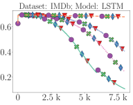
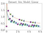
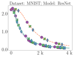
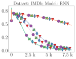
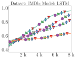
The first and second rows illustrate the loss values for the different tested models, across the datasets (columns). For the Iris dataset (first column), both the Linear model and the MLP show that the proposed HL method (represented by green crosses and blue diamonds) aligns perfectly with the loss value of the out-of-the-box gradient descent (GD) methods (purple circles) in all the tested learning configurations (GD-a/b and Mom-a/b – various dashed lines). The same trend is observed in the MNIST dataset (second column) for the ResNet and ViT models, where HL maintains a loss value comparable to other GD methods. On the IMDb dataset (third column), both the RNN and LSTM models using HL also exhibit identical loss convergence dynamics to the ones of established GD techniques. Figure 4 focuses on accuracy. In the Iris dataset, the linear model and MLP achieve accuracy levels with HL that are consistent with those of the other methods. This consistency is further demonstrated in the MNIST dataset for the ResNet and ViT models, where HL’s accuracy exactly recovers the one of other gradient descent approaches. For the IMDb dataset, both the RNN and LSTM models show that HL achieves accuracy identical to the traditional methods.

Quantitative Numerical Differences.   The starting point of the optimization is the same for all the compared cases, of course. We measured the numerical difference in weights values at the final training step, comparing the values attained by proposed HL method and the out-of-the-box gradient descent methods. In details, we compared the mean, min, max absolute differences of weights. It is numerically zero in most cases or within the order of round-off error. The Mom-a learning configuration is the only one which presented barely measurable differences, that are in the order of $\approx 1.0e^{-10}$ for the mean and absolute weight value difference, for all the considered models and settings. This indicates that HL produces the same model parameters, further supporting how it can generalize traditional optimization methods.

Refer to caption
Refer to caption
Refer to caption
Refer to caption
Refer to caption
Refer to caption
Refer to caption
Figure 3: Experimental comparisons, Loss Values. We report the outcome of comparing gradient-based learning (with and without momentum, denoted with GD and Mom, respectively) using popular out-of-the-box tools (we tested two different configurations, denoted with the suffix ”-a” and ”-b”, respectively, having different learning rates, momentum terms, damping factors) and Hamiltonian Learning (HL, setting $\tau$, $\beta$, $\eta$, $\phi$ to values that we theoretically show to be coherent with the parameters of out-of-the-box tools– see Appendix D). When considering HL, we can implement the selected model by solely considering the output function (output), the state function (state), or we can split it putting a portion into the state and a portion into the output (state/output). The plot shows the perfect alignment in terms of cost function values during the models’ training phase ($x$-axis, training steps).
Refer to caption
Refer to caption
Refer to caption
Refer to caption
Refer to caption
Refer to caption
Refer to caption
Figure 4: Experimental comparisons, Accuracy. Same setting of Figure 3. The plot shows the perfect alignment in terms of accuracy values during the models’ training phase ($x$-axis, training steps).

Appendix E Feed-forward Networks and State Net

When implementing a feed-forward network using the state network, we rely on the instantaneous propagation of Eq. 10. We get

$$\begin{split}\mathrm{\bf h}_{t+\tau}&=\mathrm{\bf h}_{t}+\tau\cdot\tau^{-1}\left(-{\mathrm{\bf h}}_{t}+{\hat{f}^{{\mathrm{\bf h}}}}(\mathrm{\bf u}_{t},{\mathrm{\bf h}}_{t},{\textpdfrender{TextRenderingMode=FillStroke,LineWidth=.4pt,}{\theta}}^{{\mathrm{\bf h}}}_{t})\right)\\ &={\hat{f}^{{\mathrm{\bf h}}}}(\mathrm{\bf u}_{t},\mathrm{\bf h}_{t},{\textpdfrender{TextRenderingMode=FillStroke,LineWidth=.4pt,}{\theta}}^{{\mathrm{\bf h}}}_{t})\end{split}.$$ (31)

In order to avoid dependencies from the past, we clear the state, $\mathrm{\bf h}_{t}={\mathrm{\bf 0}}$ and, since $\dot{{\mathrm{\bf h}}}_{t}=\tau^{-1}(-{\mathrm{\bf h}}_{t}+{\hat{f}^{{\mathrm{\bf h}}}}(\mathrm{\bf u}_{t},{\mathrm{\bf h}}_{t},{\textpdfrender{TextRenderingMode=FillStroke,LineWidth=.4pt,}{\theta}}^{{\mathrm{\bf h}}}_{t}))$, we get $\dot{{\mathrm{\bf h}}}_{t}=\tau^{-1}{\hat{f}^{{\mathrm{\bf h}}}}(\mathrm{\bf u}_{t},{\mathrm{\bf h}}_{t},{\textpdfrender{TextRenderingMode=FillStroke,LineWidth=.4pt,}{\theta}}^{{\mathrm{\bf h}}}_{t})$. Comparing this last equation with Eq. 31, we obtain

$$\begin{split}\mathrm{\bf h}_{t+\tau}&={\hat{f}^{{\mathrm{\bf h}}}}(\mathrm{\bf u}_{t},{\mathrm{\bf h}}_{t},{\textpdfrender{TextRenderingMode=FillStroke,LineWidth=.4pt,}{\theta}}^{{\mathrm{\bf h}}}_{t})=\tau\dot{{\mathrm{\bf h}}}_{t}\end{split}.$$ (32)

which is the same as Eq. 13. Finally, Eq. 14 is trivially obtained from Eq. $\mathcal{E}$ $\star$3, setting $\mathcal{\bf z}_{t}=\mathrm{\bf 0}$, to avoid propagating past information.

Appendix F Learning in Recurrent Networks

Learning in Recurrent Neural Networks (RNNs) is usually instantiated with the goal of minimizing a loss function defined on a window of sequential samples whose extremes are $a$ and $b$, with $b\geq a$, such as $\sum_{\kappa=a}^{b}L(\mathrm{\bf h}_{\kappa},\hat{\mathrm{\bf y}}_{\kappa})$, where $\mathrm{\bf h}_{\kappa}$ is the hidden state at step $\kappa$. Weights are constant while processing the data of the window. Let us consider the case of a dataset of sequences, sampled in a stochastic manner, and let us assume that at a certain stage of the optimization the values of the weights of the RNN are indicated with ${\textpdfrender{TextRenderingMode=FillStroke,LineWidth=.4pt,}{\theta}}$, while $a=1$ and $b$ is the sequence length. Once gradients $\partial\sum_{\kappa=a}^{b}L(\mathrm{\bf h}_{\kappa},\hat{\mathrm{\bf y}}_{\kappa})/\partial{\textpdfrender{TextRenderingMode=FillStroke,LineWidth=.4pt,}{\theta}}$ are computed, weights are updated following the direction of the negative gradient.

Even if we avoided explicitly showing the dependence of $L$ on ${\textpdfrender{TextRenderingMode=FillStroke,LineWidth=.4pt,}{\theta}}$, to keep the notation simple, the loss function at step $\kappa$, i.e., $L(\mathrm{\bf h}_{\kappa},\hat{\mathrm{\bf y}}_{\kappa})$, depends on ${\textpdfrender{TextRenderingMode=FillStroke,LineWidth=.4pt,}{\theta}}$ both due to its direct involvement into the computation of the current hidden state $\mathrm{\bf h}_{\kappa}$ and also through all the previous states, up to $\mathrm{\bf h}_{a}$. When applying the chain rule, following the largely known BackPropagation Through Time (BPTT) [17], we get,

$$\begin{split}\frac{\partial\sum_{\kappa=a}^{b}L(\mathrm{\bf h}_{\kappa},\hat{\mathrm{\bf y}}_{\kappa})}{\partial{\textpdfrender{TextRenderingMode=FillStroke,LineWidth=.4pt,}{\theta}}}&=\sum_{\kappa=a}^{b}\frac{\partial{L(\mathrm{\bf h}_{\kappa},\hat{\mathrm{\bf y}}_{\kappa})}}{\partial{{\textpdfrender{TextRenderingMode=FillStroke,LineWidth=.4pt,}{\theta}}}}\\ &=\sum_{\kappa=a}^{b}\sum_{q=a}^{\kappa}\frac{\partial{L(\mathrm{\bf h}_{\kappa},\hat{\mathrm{\bf y}}_{\kappa})}}{\partial\mathrm{\bf h}_{\kappa}}\frac{\partial\mathrm{\bf h}_{\kappa}}{\partial{\mathrm{\bf h}_{q}}}\frac{\partial\mathrm{\bf h}_{q}}{\partial{{\textpdfrender{TextRenderingMode=FillStroke,LineWidth=.4pt,}{\theta}}}}\\ &=\sum_{q=a}^{b}\left(\sum_{\kappa=q}^{b}\frac{\partial{L(\mathrm{\bf h}_{\kappa},\hat{\mathrm{\bf y}}_{\kappa})}}{\partial\mathrm{\bf h}_{\kappa}}\frac{\partial\mathrm{\bf h}_{\kappa}}{\partial{\mathrm{\bf h}_{q}}}\right)\frac{\partial\mathrm{\bf h}_{q}}{\partial{{\textpdfrender{TextRenderingMode=FillStroke,LineWidth=.4pt,}{\theta}}}},\end{split}$$ (33)

where in the last derivation we swapped the order of the two sums in $\kappa$ and $q$, adjusting the extremes of the summations. This can be easily done while noticing that the two summations in $\kappa$ and $q$ are represent the sum of the elements on a triangular matrix (lower triangular, if $\kappa$ is the row index), thus we can sum on rows or columns first, interchangeably. We grouped some terms in brackets since the ${\partial\mathrm{\bf h}_{q}}/{\partial{{\textpdfrender{TextRenderingMode=FillStroke,LineWidth=.4pt,}{\theta}}}}$ does not depend on index $\kappa$. Such terms can be iteratively evaluated going backward in time, exploiting the following relation,

$$\frac{\partial\mathrm{\bf h}_{b}}{\partial\mathrm{\bf h}_{q}}=\prod_{\kappa=q+1}^{b}\frac{\partial\mathrm{\bf h}_{\kappa}}{\partial\mathrm{\bf h}_{\kappa-1}}$$ (34)

with $q<b$, that can be used to compute the gradient w.r.t. ${\textpdfrender{TextRenderingMode=FillStroke,LineWidth=.4pt,}{\theta}}$ in an iterative manner, going over the input sequence in a backward manner. In fact, from Eq. 34 we get

$$\frac{\partial\mathrm{\bf h}_{b}}{\partial\mathrm{\bf h}_{q}}=\frac{\partial\mathrm{\bf h}_{b}}{\partial\mathrm{\bf h}_{q+1}}\frac{\partial\mathrm{\bf h}_{q+1}}{\partial\mathrm{\bf h}_{q}},$$ (35)

which, starting from $q=b-1$, can be efficiently evaluated for $q=b-1,b-1,\ldots,a$. We introduce additional variables to progressively accumulate gradients, i.e., $\tilde{\mathrm{\bf h}}$ and $\tilde{{\textpdfrender{TextRenderingMode=FillStroke,LineWidth=.4pt,}{\theta}}}$, with $\tilde{\mathrm{\bf h}}_{b}=\mathrm{\bf 0}$ and $\tilde{{\textpdfrender{TextRenderingMode=FillStroke,LineWidth=.4pt,}{\theta}}}_{b}=\mathrm{\bf 0}$. For $q=b,b-1,\ldots,a$ (here we have to consider also the gradient of the loss, that is why $q$ starts from $b$), we have

$\displaystyle\tilde{\mathrm{\bf h}}_{q-1}$ $\displaystyle=\frac{\partial L(\mathrm{\bf h}_{q},\hat{\mathrm{\bf y}}_{\kappa})}{\partial\mathrm{\bf h}_{q}}+\tilde{\mathrm{\bf h}}_{q}^{T}\frac{\partial\mathrm{\bf h}_{q+1}}{\partial\mathrm{\bf h}_{q}}$ (36)
$\displaystyle\tilde{{\textpdfrender{TextRenderingMode=FillStroke,LineWidth=.4pt,}{\theta}}}_{q-1}$ $\displaystyle=\tilde{{\textpdfrender{TextRenderingMode=FillStroke,LineWidth=.4pt,}{\theta}}}_{q}+\tilde{\mathrm{\bf h}}_{q-1}^{T}\frac{\partial\mathrm{\bf h}_{q}}{\partial{{\textpdfrender{TextRenderingMode=FillStroke,LineWidth=.4pt,}{\theta}}}},$ (37)

where ${\partial\mathrm{\bf h}_{q}}/{\partial{{\textpdfrender{TextRenderingMode=FillStroke,LineWidth=.4pt,}{\theta}}}}$ can be immediately evaluated without involving data of the other time instants. Eq. 37 implements the (backward) summation on index $q$ of Eq. 33 (bottom), where the term in brackets of Eq. 33 (bottom) is $\tilde{\mathrm{\bf h}}_{q}$. The summation in such a term in brackets is what is evaluated by Eq. 36. Finally,

$$\frac{\partial\sum_{\kappa=a}^{b}L(\mathrm{\bf h}_{\kappa},\hat{\mathrm{\bf y}}_{\kappa})}{\partial{\textpdfrender{TextRenderingMode=FillStroke,LineWidth=.4pt,}{\theta}}}=\tilde{\textpdfrender{TextRenderingMode=FillStroke,LineWidth=.4pt,}{\theta}}_{a}.$$ (38)

We can compare the BPTT equations Eq. 36 and Eq. 37 with the ones from Hamiltonian Learning, Eq. 17 and Eq. 18. Before going into details of the comparison, we mention that, to get Eq. 15, we exploited

$$\begin{split}\frac{\partial\dot{\mathrm{\bf h}}_{t+\tau}}{\partial\mathrm{\bf h}_{t+\tau}}&=\tau^{-1}\frac{\partial(-\mathrm{\bf h}_{t+\tau}+{\hat{f}^{{\mathrm{\bf h}}}}(\mathrm{\bf u}_{t+\tau},\mathrm{\bf h}_{t+\tau},{\textpdfrender{TextRenderingMode=FillStroke,LineWidth=.4pt,}{\theta}}^{{\mathrm{\bf h}}}_{t+\tau}))}{\partial\mathrm{\bf h}_{t+\tau}}\\ &=\tau^{-1}\left(-I+\frac{\partial\mathrm{\bf h}_{t+2\tau}}{\partial\mathrm{\bf h}_{t+\tau}}\right),\end{split}$$ (39)

and we considered $s=1$. Similarly, to get Eq. 16 we exploited

$$\frac{\partial\dot{\mathrm{\bf h}}_{t}}{\partial{\textpdfrender{TextRenderingMode=FillStroke,LineWidth=.4pt,}{\theta}}^{{\mathrm{\bf h}}}_{t}}=\tau^{-1}\frac{\partial(-\mathrm{\bf h}_{t}+{\hat{f}^{{\mathrm{\bf h}}}}(\mathrm{\bf u}_{t},\mathrm{\bf h}_{t},{\textpdfrender{TextRenderingMode=FillStroke,LineWidth=.4pt,}{\theta}}^{{\mathrm{\bf h}}}_{t}))}{\partial{\textpdfrender{TextRenderingMode=FillStroke,LineWidth=.4pt,}{\theta}}^{{\mathrm{\bf h}}}_{t}}=\tau^{-1}\frac{\partial\mathrm{\bf h}_{t+\tau}}{\partial{\textpdfrender{TextRenderingMode=FillStroke,LineWidth=.4pt,}{\theta}}^{{\mathrm{\bf h}}}_{t}},$$ (40)

since $\mathrm{\bf h}_{t}$ does not depend on ${\textpdfrender{TextRenderingMode=FillStroke,LineWidth=.4pt,}{\theta}}^{{\mathrm{\bf h}}}_{t}$ (again, $s=-1$). Going back to the comparison between the BPTT equations Eq. 36 and Eq. 37 and the ones from Hamiltonian Learning, Eq. 17 and Eq. 18, we notice that the gradient accumulators $\tilde{\mathrm{\bf h}}$ and $\tilde{{\textpdfrender{TextRenderingMode=FillStroke,LineWidth=.4pt,}{\theta}}}$ play the same role of the costates $\mathcal{\bf z}$ and $\textpdfrender{TextRenderingMode=FillStroke,LineWidth=.4pt,}{\omega}^{\mathrm{\bf h}}$, respectively. BPTT proceeds backward, while Hamiltonian Learning goes forward, processing the sequence in reverse order. Thus, $\mathcal{\bf z}_{t+\tau}$ and $\mathcal{\bf z}_{t}$ correspond to $\tilde{\mathrm{\bf h}}_{q-1}$ and $\tilde{\mathrm{\bf h}}_{q}$, respectively (same comment for the case of $\textpdfrender{TextRenderingMode=FillStroke,LineWidth=.4pt,}{\omega}^{\mathrm{\bf h}}$ and $\tilde{\textpdfrender{TextRenderingMode=FillStroke,LineWidth=.4pt,}{\theta}}$). In Hamiltonian Learning, we need to recover the states stored when processing the original sequence, thus all the $\mathrm{\bf h}$ terms involve map $\psi$ applied to time $t$. Target $\hat{\mathrm{\bf y}}_{\kappa}$ is associated to $\hat{\mathrm{\bf y}}_{\psi_{t}-\tau}$, showing that the time index of $\hat{\mathrm{\bf y}}$ is precedent with respect to the one of $\mathrm{\bf h}$ in the loss function. This is coherent with what we did when implementing feed-forward nets with the state network, Eq. 14, where we have the same offset between the times of $\mathrm{\bf h}$ and $\hat{\mathrm{\bf y}}$. Setting $\phi_{t}=\tau^{-1}$, and no dissipation ($\eta=0$), the correspondence between the two pairs of equations is perfect (i.e. the pairs of BPTT equations and the pairs of the costate-related Hamiltonian Learning equations).