A multiscale approach to the stationary Ginzburg–Landau equations of superconductivity

Christian Döding Institute for Numerical Simulation, University of Bonn, 53115 Bonn, Germany doeding@ins.uni-bonn.de Benjamin Dörich Institute for Applied and Numerical Mathematics, Karlsruhe Institute of Technology, 76149 Karlsruhe, Germany benjamin.doerich@kit.edu  and  Patrick Henning Department of Mathematics, Ruhr-University Bochum, 44801 Bochum, Germany patrick.henning@rub.de
Abstract.

In this work, we study the numerical approximation of minimizers of the Ginzburg–Landau free energy, a common model to describe the behavior of superconductors under magnetic fields. The unknowns are the order parameter, which characterizes the density of superconducting charge carriers, and the magnetic vector potential, which allows to deduce the magnetic field that penetrates the superconductor. Physically important and numerically challenging are especially settings which involve lattices of quantized vortices which can be formed in materials with a large Ginzburg–Landau parameter $\kappa$. In particular, $\kappa$ introduces a severe mesh resolution condition for numerical approximations. In order to reduce these computational restrictions, we investigate a particular discretization which is based on mixed meshes where we apply a Lagrange finite element approach for the vector potential and a localized orthogonal decomposition (LOD) approach for the order parameter. We justify the proposed method by a rigorous a-priori error analysis (in $L^{2}$ and $H^{1}$) in which we keep track of the influence of $\kappa$ in all error contributions. This allows us to conclude $\kappa$-dependent resolution conditions for the various meshes and which only impose moderate practical constraints compared to a conventional finite element discretization. Finally, our theoretical findings are illustrated by numerical experiments.

Key words and phrases:
Ginzburg–Landau equation, superconductivity, error analysis, finite element method
2020 Mathematics Subject Classification:
Primary: 65N12, 65N15. Secondary: 65N30, 35Q56
The first author is funded by the Deutsche Forschungsgemeinschaft (DFG, German Research Foundation) under Germany’s Excellence Strategy – EXC-2047/1 – 390685813. The second author is funded by the Deutsche Forschungsgemeinschaft (DFG, German Research Foundation) – Project-ID 258734477 – SFB 1173. The third authors also acknowledges the support by the Deutsche Forschungsgemeinschaft through the grant HE 2464/7-1.

1. Introduction

In most materials the flow of an electric current is countered with an electric resistance which leads to a loss in energy. Materials with no electrical resistance, usually referred to as superconductors, are rare in nature, but open up a large variety of possible applications. To consider a mathematical model for superconductivity, we let $\Omega\subset\mathbb{R}^{3}$ denote a cuboid which is occupied by the superconducting material. The superconductivity itself is described by a complex-valued wave function $u\colon\Omega\rightarrow\mathbb{C}$ which is called the order parameter. Though not a physical observable on its own, we can extract from $u$ the density of the superconducting electron pairs $|u|^{2}$. This density is real-valued and can be observed in physical experiments. In fact, the scaling in the corresponding models enforces $0\leq|u|^{2}\leq 1$, where $|u(x)|^{2}=0$ implies that the material is not superconducting (in normal state) in $x\in\Omega$ and $|u(x)|^{2}=1$ implies a perfect superconductor, locally in $x$. In between, the percentage of superconducting charge carriers might drop to a value between 00 and $1$. In these mixed normal-superconducting states, both phases can coexist in a so-called Abrikosov vortex lattice [Abr04] with $|u(x)|^{2}=0$ in the vortex centers. These kind of configurations can only occur for so-called type-II superconductors when a sufficiently strong (but not too strong) external magnetic field $\mathbf{H}$ is applied. In fact, in mixed normal-superconducting states, the magnetic field partially penetrates the superconducting material. In this paper, we focus on exactly these kind of settings.

Considering such a situation, the relevant order parameter and the unknown internal magnetic field can be characterized as minimzers of the so-called Ginzburg–Landau (GL) free energy (cf. [DuGP92, Sec. 3]), which is given by

(1.1) $\displaystyle E_{\mbox{\tiny GL}}(u,\mathbf{A})$ $\displaystyle\coloneqq$ $\displaystyle\frac{1}{2}\int_{\Omega}|\frac{\mathrm{i}}{\kappa}\nabla u+\mathbf{A}u|^{2}+\frac{1}{2}\bigl{(}1-|u|^{2}\bigr{)}^{2}+|\operatorname{curl}\mathbf{A}-\mathbf{H}|^{2}\,\,\mbox{d}x.$

Here, $\mathbf{H}$ is a given external magnetic field and $\kappa\in\mathbb{R}^{+}$ is a material parameter, often called the Ginzburg–Landau parameter. The unknown $\mathbf{A}$ denotes the magnetic vector potential, from which we can obtain the internal magnetic field given by $\operatorname{curl}\mathbf{A}$. In fact, besides the density $|u|^{2}$, the magnetic field $\operatorname{curl}\mathbf{A}$ is the second physical quantity of interest. Recalling that we are interested in vortex states, it is important to note that the size of the parameter $\kappa$ determines the structure of the vortex lattice [SaS07, SaS12, Ser99, SeS10]. In particular, for small values of $\kappa$, no vortices will appear, whereas with increasing $\kappa$, the number of vortices grows and they become more localized [Aftalion99, SaS07]. Thus, the regime of large values of $\kappa$ is the physically most interesting regime accompanied by many challenges for its numerical approximation. The phenomenon is also closely related to the appearance of vortices in superfluids [Du2003].

First results on the numerical approximation of minimizers to (1.1) were obtained in the pioneering works by Du, Gunzburger and Peterson [DuGP92, DuGP93] who derived $H^{1}$-error estimates in finite element (FE) spaces for both the order parameter $u$ and the magnetic vector potential $\mathbf{A}$. Even though estimates of optimal convergence order could be provided in a (joint) mesh parameter $H$, the proof techniques could not take into account the precise role of $\kappa$ and how it affects potential constraints on the mesh size for $u$ and $\mathbf{A}$ respectively. An error analysis for alternative discretizations based on a covolume method [DuNicolaidesWu98] or a finite volume method [QuJu05] can be also found in the literature. However, both works only establish convergence, but no rates in $H$ and $\kappa$.

First error estimates that are indeed explicit with respect to $\kappa$ and the mesh size $H$ were recently obtained in [DoeH24] for a finite element discretization of (1.1), however, in a simplified setting where the vector potential $\mathbf{A}$ was assumed to be given and the minimization of the energy only involved $u$. In this case, the last term in (1.1) can be dropped. In the aforementioned work, it was found that the mesh size $H$ needs to fulfill a resolution condition of at least $H\lesssim\kappa^{-1}$ to obtain reliable approximations. Even more, the error estimates indicated a pre-asymptotic convergence regime, subject to a second resolution condition that depends on the strength of local convexity of $E_{\mbox{\tiny GL}}$ in a neighborhood of a minimizer, i.e., on the smallest eigenvalues of $E_{\mbox{\tiny GL}}^{\prime\prime}(u)$. In fact, the numerical experiments indicated that this resolution condition is not an artifact of the analysis, but FE spaces with too coarse meshes are not able to capture the correct vortex patterns, which leads to significant practical constraints.

To overcome these constraints it was suggested in [DoeH24] to use a discretization based on Localized Orthogonal Decomposition (LOD). This idea was later realized in [BDH24] (still in the setting of given $\mathbf{A}$). The LOD is a numerical homogenization technique designed by Målqvist and Peterseim [MaP14] to tackle elliptic multiscale problems. In the last decade it was generalized multiple times and applied to a large variety of different problems, were we exemplary refer to [DoHaMa23, DHW24, GHV17, EHMP19, HaP23, HeP13, LaLjMa24, LjMaMa22, MaPer18, Mai21, MaVer22, Pet17, WuZh22] and the reference therein, as well as to the reviews given in [AHP21acta] and [MaP21]. Applying the LOD to approximate minimizers of the Ginzburg–Landau energy can be motivated with its fast convergence under comparably weak regularity assumptions. This is achieved by constructing an approximation space (the LOD space) that contains problem-specific information, in particular it is based on $\kappa$ and $\mathbf{A}$. A comprehensive error analysis of the resulting method was given in [BDH24], revealing that the $\kappa$-dependent resolution conditions can be indeed relaxed with this strategy and correct vortex patters could be computed on rather coarse meshes. Furthermore, the locality for the LOD shape functions was quantified, where it was found that approximate shape functions with a diameter of order $\mathcal{O}(\log(H\kappa)H)$ are sufficient to preserve the overall approximation properties of the ideal LOD method. However, in the aforementioned work the LOD spaces were computed in an offline phase and the error analysis was only carried out for the simplified energy under the assumption that the vector potential $\mathbf{A}$ is a-priori known and not part of the minimization process.

Turning to the full problem (1.1), one would naively try and use an LOD approach on both $u$ and $\mathbf{A}$. However, this is computationally extremely expensive and, as one can see from our error analysis and numerical experiments, there is typically no need for a fine resolution of the vector potential $\mathbf{A}$. This motivates one of the main questions of this work: What are suitable, possibly different discretizations of the pair $(u,\mathbf{A})$ such that we can achieve high convergence rates under possibly low regularity assumptions and weak resolution conditions and can we quantify the corresponding error if different ansatz spaces are used for $u$ and $\mathbf{A}$? The key in the error analysis of [DoeH24] was a detailed a-priori analysis of the continuous and discrete minimizers in order to obtain bounds which are sharp in their $\kappa$-scaling. Following this approach, we generalize these techniques and derive bounds for continuous and discrete minimizers which are explicit in $\kappa$. Most notably, we show that the bounds on $u$ in Sobolev norms depend on $\kappa$ whereas the bounds on $\mathbf{A}$ up to its second derivative are independent of $\kappa$, which resembles the simpler structure of $\mathbf{A}$ even in large $\kappa$-regimes. Denoting by $H$ and $h$ the spatial mesh size of the discrete spaces for $u$ and $\mathbf{A}$ respectively, our error bounds allow us to extract optimal coupling conditions between $H$ and $h$ depending on the polynomial degree of the FE space and the parameter $\kappa$. The main challenge is the intrinsic coupling of $u$ and $\mathbf{A}$ within the energy and the Fréchet derivatives. Here, again it turned out to be crucial to work with appropriately scaled norms for both quantities in order to derive sharp estimates in $\kappa$. Also in the error analysis we need to carefully balance the distribution of regularity and integrability in our estimates such that no superfluous powers of $\kappa$ enter the final error bounds. Our experiments then indeed confirm that these bounds are optimal with one minor exception. In our theory, the $H^{3}$-norm of $\mathbf{A}$ is expected to grow linearly in $\kappa$ which is not visible in the experiments. To us it remains open whether this is an artifact of the analysis or other examples could support our theory. We note that we chose $\Omega$ as a cuboid to obtain all necessary regularity estimates in a rigorous way even without assuming a smooth boundary.

Finally, let us mention that there has also been a lot of work on the time-dependent Ginzburg–Landau equations which typically has a gradient flow structure and which is used to describe the dynamics within a superconductor. Corresponding numerical methods, convergence results and error estimates can be for example found in [Bartels2005, Bar05, BarMO11, Chen97, CheD01, Du94b, Du94, Du97, DuGray96, DuanZhang22, GJX19, GaoS18, Li17, LiZ15, LiZ17, MaQ23] and the references therein. To the best of our knowledge, questions regarding vortex-resolution conditions depending on $\kappa$ and $\mathbf{A}$ have not yet been studied in the time-dependent case. Due to the different nature of the time-dependent problem, we will not discuss the equation any further here.

The rest of the paper is organized as follows: In Section 2, we introduce the analytical framework and present several results on a-priori bounds and the regularity of the continuous minimizers. Furthermore, we discuss the gauge conditions and study the resulting properties of the Fréchet derivatives. The core findings of our paper are stated in Section 3. Here we present the construction of LOD spaces in our problem setting together with our corresponding main results. The main results are proved step by step in the sections after. First, in Section 4, we provide further analytical findings which are crucial for the later error estimates. An abstract error analysis is then established in Section 5. Finally, the abstract results are applied in Section 6 to the considered LOD discretization and we give the corresponding proofs to our main results. Numerical experiments which illustrate our theoretical findings are shown in Section 7. The regularity theory and technical computations are postponed to the Appendices A and B.

Notation

For a complex number $z\in\mathbb{C}$, we use $z^{*}$ for the complex conjugate of $z$. In the whole paper we further denote by $L^{2}(\Omega):=L^{2}(\Omega,\mathbb{C})$ the Hilbert space of $L^{2}$-integrable complex functions, but equipped with the real scalar product $m(u,v):=\operatorname{Re}\int_{\Omega}v\,w^{*}\,dx$ for $v,w\in L^{2}(\Omega)$. Hence, we interpret the space as a real Hilbert space. Analogously, we equip the space $H^{1}(\Omega):=H^{1}(\Omega,\mathbb{C})$, which will be the solution space for the order parameter, with the scalar product $m(v,w)+m(\nabla v,\nabla w)$. This interpretation is crucial so that the Fréchet derivatives of $E$ are meaningful and exist on $H^{1}(\Omega)$. For any space $X$, we denote its dual space by $X^{\prime}$. Note that this implies, that the elements of the dual space of $H^{1}$ consist of real-linear functionals, which are not necessarily complex-linear. For example, if $F(v):=m(f,v)$ for some $f\in L^{2}(\Omega)$, then it holds $F(\alpha\,v)=\alpha\,F(v)$ if $\alpha\in\mathbb{R}$, but in general not if $\alpha\in\mathbb{C}$.

For the real-valued vector potentials, we use boldface letters and denote $\mathbf{L}^{2}(\Omega):=L^{2}(\Omega;\mathbb{R}^{3})$ and $\mathbf{H}^{1}(\Omega)\coloneqq H^{1}(\Omega;\mathbb{R}^{3})$. Note that functions in $H^{1}(\Omega)$ are complex-valued, whereas functions in $\mathbf{H}^{1}(\Omega)$ are real-valued. Analogously, we transfer the notation to higher order Sobolev spaces, i.e., $H^{k}(\Omega)\coloneqq H^{k}(\Omega;\mathbb{C})$ and $\mathbf{H}^{k}(\Omega)\coloneqq H^{k}(\Omega;\mathbb{R}^{3})$ for $k\in\mathbb{N}_{0}$. Further, we use the standard spaces for the weak rotation and divergence, i.e., $\mathbf{H}(\operatorname{curl})=\mathbf{H}(\operatorname{curl},\Omega)$ and $\mathbf{H}(\operatorname{div})=\mathbf{H}(\operatorname{div},\Omega)$, both for real-valued functions.

Throughout the paper $C$ denotes a generic constant which is independent of $\kappa$ and the spatial mesh parameters $H$ and $h$, but might depend on numerical constants as well as $\Omega$ and $\mathbf{H}$. In particular, we write $\alpha\lesssim\beta$ if there is a constant $C$ independent of $\kappa$, $H$ and $h$ such that $\alpha\leq C\,\beta$.

2. Analytical framework

In the following, recall that $\Omega\subset\mathbb{R}^{3}$ denotes the computational domain which we assume to be a rectangular cuboid. For the naturally appearing boundary conditions of minimizers as well as the gauging process, we additionally introduce the subspace of $\mathbf{H}^{1}(\Omega)$ of functions with vanishing normal trace as

(2.1) $\displaystyle\mathbf{H}^{1}_{\mathrm{n}}(\Omega)$ $\displaystyle\coloneqq$ $\displaystyle\{\,\mathbf{B}\in\mathbf{H}^{1}(\Omega)\,\mid\,\mathbf{B}\cdot\nu|_{\partial\Omega}=0\,\}.$

Among all order parameters $u\in H^{1}(\Omega)$ and vector potentials $\mathbf{A}\in\mathbf{H}^{1}(\Omega)$, we are interested in finding a pair that minimizes the Ginzburg–Landau free energy in (1.1) with a given external magnetic field $\mathbf{H}\in\mathbf{H}(\operatorname{curl})$ and a material parameter $\kappa\in\mathbb{R}^{+}$. In this setting, we seek $(u,\mathbf{A})\in H^{1}(\Omega)\times\mathbf{H}^{1}(\Omega)$ such that

$\displaystyle E_{\mbox{\tiny GL}}(u,\mathbf{A})$ $\displaystyle=$ $\displaystyle\inf_{(v,\mathbf{B})\in H^{1}(\Omega)\times\mathbf{H}^{1}(\Omega)}E_{\mbox{\tiny GL}}(v,\mathbf{B}).$

It is well known that minimizers cannot be unique since the GL energy functional $E_{\mbox{\tiny GL}}$ is invariant under certain gauge transformations [DuGP92]. To be precise, for any (real-valued) $\phi\in H^{2}(\Omega;\mathbb{R})$ we define the corresponding gauge transformation $G_{\phi}:H^{1}(\Omega)\times\mathbf{H}^{1}(\Omega)\rightarrow H^{1}(\Omega)\times\mathbf{H}^{1}(\Omega)$ by

(2.2) $\displaystyle G_{\phi}(u,\mathbf{A})\coloneqq(u\,e^{\mathrm{i}\kappa\phi},\mathbf{A}+\nabla\phi).$

It is easily checked that $E_{\mbox{\tiny GL}}$ is gauge invariant in the sense that

$\displaystyle E_{\mbox{\tiny GL}}(u,\mathbf{A})=E_{\mbox{\tiny GL}}(\,G_{\phi}(u,\mathbf{A})\,)\qquad\mbox{for all }\enspace(u,\phi,\mathbf{A})\in H^{1}(\Omega)\times H^{2}(\Omega)\times\mathbf{H}^{1}(\Omega).$

Hence, if $(u,\mathbf{A})$ is a minimizer, then $G_{\phi}(u,\mathbf{A})$ is a minimizer, too. For smooth domains, it can be shown that any pair $(u,\mathbf{A})\in H^{1}(\Omega)\times\mathbf{H}^{1}(\Omega)$ is gauge equivalent to a pair $(v,\mathbf{B})\in H^{1}(\Omega)\times\mathbf{H}^{1}(\Omega)$ where the corresponding vector potential $\mathbf{B}$ is divergence-free and has a vanishing normal trace, cf. [DuGP92, Lemma 3.1]. To be precise, let $\phi\in H^{1}(\Omega;\mathbb{R})$ denote the zero-average solution to the Poisson problem $-\Delta\phi=-\operatorname{div}\mathbf{A}$ with inhomogeneous Neumann boundary condition $\nabla\phi\cdot\nu|_{\partial\Omega}=\mathbf{A}\cdot\nu|_{\partial\Omega}$, then it holds $\phi\in H^{2}(\Omega;\mathbb{R})$ (this follows by combining the results of [Grisvard85, Theorem 3.2.1.3] and [GirR86, Lemma 3.7 and Theorem 3.9] and by decomposing $\phi$ accordingly into an affine contribution, a solution to a homogeneous Poisson problem with inhomogeneous Neumann boundary condition and a solution to an inhomogeneous Poisson problem with homogeneous Neumann boundary condition). With this, we have $G_{\phi}(u,\mathbf{A})\in H^{1}(\Omega)\times\mathbf{H}^{1}_{\mathrm{n},\operatorname{div}}(\Omega)$ where

$\displaystyle\mathbf{H}^{1}_{\mathrm{n},\operatorname{div}}(\Omega)\coloneqq\{\,\mathbf{B}\in\mathbf{H}^{1}(\Omega)\,\mid\,\operatorname{div}\mathbf{B}=0\,\mbox{ and }\,\mathbf{B}\cdot\nu|_{\partial\Omega}=0\,\}.$

As a direct conclusion, we can, without loss of generality, restrict the minimization of $E_{\mbox{\tiny GL}}$ to functions in $H^{1}(\Omega)\times\mathbf{H}^{1}_{\mathrm{n},\operatorname{div}}(\Omega)$. This corresponds to the Coulomb gauge of the vector potentials. Furthermore, if we restrict the vector potentials to divergence-free functions then they are only gauge equivalent to itself. In particular, if $(u,\mathbf{A}),(v,\mathbf{B})\in H^{1}(\Omega)\times\mathbf{H}^{1}_{\mathrm{n},\operatorname{div}}(\Omega)$, then

$\displaystyle G_{\phi}(u,\mathbf{A})=(v,\mathbf{B})\qquad\Longleftrightarrow\qquad\mathbf{A}=\mathbf{B}\,\,\mbox{ and }\,\,v=u\,e^{\mathrm{i}\kappa\phi}\mbox{ for }\phi\in\mathbb{R}.$

This equivalence is easily seen by the observation that if $\operatorname{div}\mathbf{A}=0$ and $\operatorname{div}(\mathbf{A}+\nabla\phi)=\operatorname{div}\mathbf{B}=0$, then $\Delta\phi=0$ with $\nabla\phi\cdot\nu=\mathbf{A}\cdot\nu=0$ on $\partial\Omega$, hence, $\phi$ must be a constant and the gauge transform reduces to $G_{\phi}(u,\mathbf{A})=(u\,e^{\mathrm{i}\kappa\phi},\mathbf{A})$ on $H^{1}(\Omega)\times\mathbf{H}^{1}_{\mathrm{n},\operatorname{div}}(\Omega)$. Since minimization over divergence-free functions can be cumbersome in practice, the energy can be stabilized by a penalty term that depends on the divergence of a vector field. We therefore define

(2.3) $$E(u,\mathbf{A})\,:=\,E_{\mbox{\tiny GL}}(u,\mathbf{A})+\frac{1}{2}\int_{\Omega}|\operatorname{div}\mathbf{A}|^{2}\,\textup{d}x$$

and observe that any minimizer of $E$ must be also a minimizer of $E_{\mbox{\tiny GL}}$ and, vice versa, any minimizer of $E_{\mbox{\tiny GL}}$ is gauge-equivalent to a minimizer of $E$ for which $\operatorname{div}\mathbf{A}=0$ holds. In the following, we can therefore restrict our analysis to the minimization of the stabilized energy $E$. The existence of minimizers was proved by Du et al. [DuGP92] and we have the following result.

Theorem 2.1 ([DuGP92, Thm. 3.8]).

There exists at least one minimizer of the energy (2.3), i.e., there is $(u,\mathbf{A})\in H^{1}(\Omega)\times\mathbf{H}^{1}_{\mathrm{n}}(\Omega)$ such that

(2.4) $\displaystyle(u,\mathbf{A})=\underset{(v,\mathbf{B})\in H^{1}(\Omega)\times\mathbf{H}^{1}_{\mathrm{n}}(\Omega)}{\mbox{arg\,min}}E(v,\mathbf{B}).$

In particular, for any minimizer $(u,\mathbf{A})$ the vector potential $\mathbf{A}$ satisfies $\operatorname{div}\mathbf{A}=0$, and thus also minimizes (1.1).

The result remains valid for external fields $\mathbf{H}\in\mathbf{L}^{2}(\Omega)$.

As discussed above, the modification of the energy functional from $E_{\mbox{\tiny GL}}$ to $E$ restricts the gauge transforms to divergence-free vector fields, which in turn implies that the gauge transforms $G_{\phi}(u,\mathbf{A})$ in (2.2) are only admissible if $\phi$ is a constant real number. Consequently, we call $(u,\mathbf{A})\in H^{1}(\Omega)\times\mathbf{H}^{1}_{\mathrm{n}}(\Omega)$ gauge equivalent to $(v,\mathbf{B})\in H^{1}(\Omega)\times\mathbf{H}^{1}_{\mathrm{n}}(\Omega)$ for $E$, if and only if $\mathbf{A}=\mathbf{B}$ and

(2.5) $\displaystyle v=u\,e^{\mathrm{i}\omega}\,\,\,\mbox{ for some }\omega\in[-\pi,\pi).$

Note that $\omega$ corresponds to $\kappa\phi$ in (2.2).

2.1. Fréchet derivatives and stability bounds

Crucial components of our error analysis are the derivatives of the energy and corresponding first- and second-order conditions for minimizers. In the following, we start with summarizing the arising Fréchet derivatives of $E$, where we refer to [DuGP92, Section 3.3].

Lemma 2.2.

Let $E$ denote the energy functional given by (2.3), then $E$ is (infinitely) Fréchet differentiable where, for any $(u,\mathbf{A})\in H^{1}(\Omega)\times\mathbf{H}^{1}_{\mathrm{n}}(\Omega)$, the first partial derivatives

$\displaystyle\partial_{u}E(u,\mathbf{A}):H^{1}(\Omega)\rightarrow\mathbb{R}\quad\mbox{and}\quad\partial_{\mathbf{A}}E(u,\mathbf{A}):\mathbf{H}^{1}_{\mathrm{n}}(\Omega)\rightarrow\mathbb{R}$

are respectively given by

(2.6) $\displaystyle\partial_{u}E(u,\mathbf{A})\varphi$ $\displaystyle=\operatorname{Re}\int_{\Omega}\bigl{(}\frac{\mathrm{i}}{\kappa}\nabla u+\mathbf{A}u\bigr{)}\cdot\bigl{(}\frac{\mathrm{i}}{\kappa}\nabla\varphi+\mathbf{A}\varphi\bigr{)}^{*}+\bigl{(}|u|^{2}-1\bigr{)}u\varphi^{*}\,\textup{d}x,$
(2.7) $\displaystyle\partial_{\mathbf{A}}E(u,\mathbf{A})\mathbf{B}$ $\displaystyle=\int_{\Omega}|u|^{2}\mathbf{A}\cdot\mathbf{B}+\frac{1}{\kappa}\operatorname{Re}\bigl{(}\mathrm{i}u^{*}\nabla u\cdot\mathbf{B}\bigr{)}+\operatorname{curl}\mathbf{A}\cdot\operatorname{curl}\mathbf{B}+\operatorname{div}\mathbf{A}\cdot\operatorname{div}\mathbf{B}-\mathbf{H}\cdot\operatorname{curl}\mathbf{B}\,\textup{d}x$

for $\varphi\in H^{1}(\Omega)$ and $\mathbf{B}\in\mathbf{H}^{1}_{\mathrm{n}}(\Omega)$.

The first order conditions for minimizers (cf. [Casas-trroeltsch-2015]) imply $E^{\prime}(u,\mathbf{A})=0$ if $(u,\mathbf{A})$ fulfils (2.4). By splitting $E^{\prime}(u,\mathbf{A})$ into $\partial_{u}E(u,\mathbf{A})$ and $\partial_{\mathbf{A}}E(u,\mathbf{A})$ we obtain the Ginzburg–Landau equations. For readability, we highlight this observation in the following lemma.

Lemma 2.3 (Ginzburg–Landau equations).

Let $(u,\mathbf{A})\in H^{1}(\Omega)\times\mathbf{H}^{1}_{\mathrm{n}}(\Omega)$ be a minimizer of problem (2.4). Then, it holds $\partial_{u}E(u,\mathbf{A})=0$ and $\partial_{\mathbf{A}}E(u,\mathbf{A})=0$. By expressing these identities in variational form, we obtain that $(u,\mathbf{A})\in H^{1}(\Omega)\times\mathbf{H}^{1}_{\mathrm{n}}(\Omega)$ solves the Ginzburg–Landau equations

$\displaystyle\operatorname{Re}\int_{\Omega}\bigl{(}\frac{\mathrm{i}}{\kappa}\nabla u+\mathbf{A}u\bigr{)}\cdot\bigl{(}\frac{\mathrm{i}}{\kappa}\nabla\varphi+\mathbf{A}\varphi\bigr{)}^{*}+\bigl{(}|u|^{2}-1\bigr{)}u\varphi^{*}\,\textup{d}x$ $\displaystyle=$ $\displaystyle 0,$
$\displaystyle\int_{\Omega}|u|^{2}\mathbf{A}\cdot\mathbf{B}+\frac{1}{\kappa}\operatorname{Re}\bigl{(}\mathrm{i}u^{*}\nabla u\cdot\mathbf{B}\bigr{)}+\operatorname{curl}\mathbf{A}\cdot\operatorname{curl}\mathbf{B}+\operatorname{div}\mathbf{A}\cdot\operatorname{div}\mathbf{B}-\mathbf{H}\cdot\operatorname{curl}\mathbf{B}\,\textup{d}x$ $\displaystyle=$ $\displaystyle 0,$

for all $\varphi\in H^{1}(\Omega)$ and $\mathbf{B}\in\mathbf{H}^{1}_{\mathrm{n}}(\Omega)$.

Next, we turn to the second partial Fréchet derivatives of $E$ which we later require for second order minimality conditions. The second derivatives of $E$ are given as follows.

Lemma 2.4.

Let $E$ be given by (2.3). For $(u,\mathbf{A})\in H^{1}(\Omega)\times\mathbf{H}^{1}_{\mathrm{n}}(\Omega)$ we denote the second order partial Fréchet derivatives by

$\displaystyle\langle\partial^{2}_{u}E(u,\mathbf{A})\,\,\cdot\,\,,\varphi\rangle$ $\displaystyle\coloneqq$ $\displaystyle\frac{\partial}{\partial u}(\partial_{u}E(u,\mathbf{A})\varphi):H^{1}(\Omega)\rightarrow\mathbb{R},$
$\displaystyle\langle\partial_{\mathbf{A},u}E(u,\mathbf{A})\,\,\cdot\,\,,\mathbf{B}\rangle$ $\displaystyle\coloneqq$ $\displaystyle\frac{\partial}{\partial u}(\partial_{\mathbf{A}}E(u,\mathbf{A})\mathbf{B}):H^{1}(\Omega)\rightarrow\mathbb{R},$
$\displaystyle\langle\partial_{u,\mathbf{A}}E(u,\mathbf{A})\,\,\cdot\,\,,\varphi\rangle$ $\displaystyle\coloneqq$ $\displaystyle\frac{\partial}{\partial\mathbf{A}}(\partial_{u}E(u,\mathbf{A})\varphi):\mathbf{H}^{1}_{\mathrm{n}}(\Omega)\rightarrow\mathbb{R},$
$\displaystyle\langle\partial^{2}_{\mathbf{A}}E(u,\mathbf{A})\,\,\cdot\,\,,\mathbf{B}\rangle$ $\displaystyle\coloneqq$ $\displaystyle\frac{\partial}{\partial\mathbf{A}}(\partial_{\mathbf{A}}E(u,\mathbf{A})\mathbf{B}):\mathbf{H}^{1}_{\mathrm{n}}(\Omega)\rightarrow\mathbb{R},$

where $\varphi\in H^{1}(\Omega)$ and $\mathbf{B}\in\mathbf{H}^{1}_{\mathrm{n}}(\Omega)$. The derivatives are given by

(2.8) $\displaystyle\langle\partial^{2}_{u}E(u,\mathbf{A})\psi,\varphi\rangle$ $\displaystyle=\operatorname{Re}\int_{\Omega}\bigl{(}\frac{\mathrm{i}}{\kappa}\nabla\varphi+\mathbf{A}\varphi\bigr{)}\cdot\bigl{(}\frac{\mathrm{i}}{\kappa}\nabla\psi+\mathbf{A}\psi\bigr{)}^{*}+\bigl{(}|u|^{2}-1\bigr{)}\varphi\psi^{*}+u^{2}\varphi^{*}\psi^{*}+|u|^{2}\varphi\psi^{*}\,\textup{d}x,$
(2.9) $\displaystyle\langle\partial^{2}_{\mathbf{A}}E(u,\mathbf{A})\mathbf{B},\mathbf{C}\rangle$ $\displaystyle=\int_{\Omega}|u|^{2}\mathbf{C}\cdot\mathbf{B}+\operatorname{curl}\mathbf{C}\cdot\operatorname{curl}\mathbf{B}+\operatorname{div}\mathbf{C}\cdot\operatorname{div}\mathbf{B}\,\textup{d}x,$
(2.10) $\displaystyle\langle\partial_{u,\mathbf{A}}E(u,\mathbf{A})\mathbf{B},\varphi\rangle$ $\displaystyle=\int_{\Omega}2\operatorname{Re}(u\varphi^{*})\mathbf{A}\cdot\mathbf{B}+\frac{1}{\kappa}\operatorname{Re}\bigl{(}\mathrm{i}u^{*}\nabla\varphi+\mathrm{i}\varphi^{*}\nabla u\bigr{)}\cdot\mathbf{B}\,\textup{d}x$

and $\langle\partial_{u,\mathbf{A}}E(u,\mathbf{A})\mathbf{B},\varphi\rangle=\langle\partial_{\mathbf{A},u}E(u,\mathbf{A})\varphi,\mathbf{B}\rangle$.

The proof follows with straightforward calculations.

In order to quantify the $\kappa$-dependencies in our error estimates, we also require suitable stability estimates for the minimzers $(u,\mathbf{A})$ of the energy (2.3). For this, we use the following $\kappa$-weighted norms throughout the paper:

(2.11a) $\displaystyle\lvert|\varphi\rvert|_{H^{1}_{\kappa}}^{2}$ $\displaystyle=$ $\displaystyle\kappa^{-2}\lvert|\nabla\varphi\rvert|_{L^{2}}^{2}+\lvert|\varphi\rvert|_{L^{2}}^{2},\hskip 30.0pt\lvert|\varphi\rvert|_{H^{2}_{\kappa}}^{2}\,\,\,=\,\,\,\kappa^{-2}\lvert|\nabla\varphi\rvert|_{H^{1}_{\kappa}}^{2}+\lvert|\varphi\rvert|_{L^{2}}^{2},$
(2.11b) $\displaystyle\lvert|\mathbf{B}\rvert|_{H^{1}}^{2}$ $\displaystyle=$ $\displaystyle\lvert|\mathbf{B}\rvert|_{L^{2}}^{2}+\lvert|\nabla\mathbf{B}\rvert|_{L^{2}}^{2},\hskip 43.0pt\lvert|\mathbf{B}\rvert|_{H^{2}}^{2}\,\,\,=\,\,\,\lvert|D^{2}\mathbf{B}\rvert|_{L^{2}}^{2}+\lvert|\mathbf{B}\rvert|_{H^{1}}^{2}.$

Here we formally define the norms that involve derivatives of the (vector-valued) functions $\mathbf{B}$ as $\lvert|\nabla\mathbf{B}\rvert|_{L^{2}}^{2}=\sum\limits_{i,k=1}^{3}\lvert|\partial_{x_{i}}\mathbf{B}_{j}\rvert|_{L^{2}}^{2}$ and $\lvert|D^{2}\mathbf{B}\rvert|_{L^{2}}^{2}=\sum\limits_{i,j,k=1}^{3}\lvert|\partial_{x_{i}x_{j}}\mathbf{B}_{k}\rvert|_{L^{2}}^{2}$.

Lemma 2.5 (Stability bounds).

Let $(u,\mathbf{A})\in H^{1}(\Omega)\times\mathbf{H}^{1}_{\mathrm{n}}(\Omega)$ be a minimizer of problem (2.4) in Theorem 2.1. Then, the following stability bounds hold

(2.12) $\displaystyle|u|\leq 1\,\text{a.e.},\quad\lvert|\tfrac{1}{\kappa}\nabla u\rvert|_{L^{2}}\lesssim\lvert|u\rvert|_{L^{2}}+\lvert|\mathbf{A}u\rvert|_{L^{2}},\quad\lvert|u\rvert|_{H^{1}_{\kappa}}\lesssim 1+\lvert|\mathbf{H}\rvert|_{L^{2}},\quad\lvert|\mathbf{A}\rvert|_{H^{1}}$ $\displaystyle\lesssim 1+\lvert|\mathbf{H}\rvert|_{L^{2}}.$
Proof.

The pointwise bound $\lvert|u\rvert|_{L^{\infty}}\leq 1$ is shown in [DuGP92, Prop. 3.11]. Next, note that

(2.13) $$E(0,\mathbf{0})=\tfrac{1}{2}\operatorname{vol}(\Omega)+\tfrac{1}{2}\lvert|\mathbf{H}\rvert|_{L^{2}}^{2},$$

and thus for any minimizer it holds

(2.14) $$\lvert|\operatorname{curl}\mathbf{A}-\mathbf{H}\rvert|_{L^{2}}^{2}+\lvert|\operatorname{div}\mathbf{A}\rvert|_{L^{2}}^{2}\lesssim 1+\lvert|\mathbf{H}\rvert|_{L^{2}}^{2}.$$

At the same time, basic manipulations give us

(2.15) $$\lvert|\operatorname{curl}\mathbf{A}\rvert|_{L^{2}}^{2}\lesssim\lvert|\operatorname{curl}\mathbf{A}-\mathbf{H}\rvert|_{L^{2}}^{2}+\lvert|\mathbf{H}\rvert|_{L^{2}}^{2}.$$

Combining the two estimates yields $\lvert|\operatorname{curl}\mathbf{A}\rvert|_{L^{2}}+\lvert|\operatorname{div}\mathbf{A}\rvert|_{L^{2}}\lesssim 1+\lvert|\mathbf{H}\rvert|_{L^{2}}$. Using [GirR86, Lemma 3.6] gives the $L^{2}$ bound, and [GirR86, Theorem 3.9] the $H^{1}$ bound on $\mathbf{A}$.

Further, we obtain with $|u|\leq 1$ the estimate

(2.16) $$\lvert|\tfrac{1}{\kappa}\nabla u\rvert|_{L^{2}}\leq\lvert|\tfrac{1}{\kappa}\nabla u+\mathrm{i}\mathbf{A}u\rvert|_{L^{2}}+\lvert|\mathbf{A}u\rvert|_{L^{2}}\lesssim 1+\lvert|\mathbf{H}\rvert|_{L^{2}}+\lvert|\mathbf{A}\rvert|_{L^{2}}\lesssim 1+\lvert|\mathbf{H}\rvert|_{L^{2}}.$$

It remains to prove the second estimate, which we obtain with Lemma 2.3 as

$\displaystyle\int_{\Omega}|\tfrac{\mathrm{i}}{\kappa}\nabla u+\mathbf{A}u|^{2}\,\,\mbox{d}x=\int_{\Omega}(1-|u|^{2})\,|u|^{2}\,\,\mbox{d}x\leq\|u\|_{L^{2}}^{2}.$

The estimate now follows with $\lvert|\tfrac{1}{\kappa}\nabla u\rvert|_{L^{2}}\leq\lvert|\tfrac{1}{\kappa}\nabla u+\mathrm{i}\mathbf{A}u\rvert|_{L^{2}}+\lvert|\mathbf{A}u\rvert|_{L^{2}}\leq\|u\|_{L^{2}}+\lvert|\mathbf{A}u\rvert|_{L^{2}}$. ∎

2.2. Higher order regularity of the minimizers

Next, we will investigate the higher order regularity of minimizers together with corresponding $\kappa$-explicit regularity bounds.

Concerning the vector potential $\mathbf{A}$, we can characterize it as the solution $\mathbf{U}\in\mathbf{H}^{1}_{\mathrm{n},\operatorname{div}}(\Omega)$ to a problem of the following form

(2.17a) $$\int_{\Omega}\operatorname{curl}\mathbf{U}\cdot\operatorname{curl}\mathbf{B}\,\,\textup{d}x=\int_{\Omega}\mathbf{F}\cdot\mathbf{B}+\mathbf{H}\cdot\operatorname{curl}\mathbf{B}\,\textup{d}x,\quad\text{for all }\mathbf{B}\in\mathbf{H}^{1}_{\mathrm{n}}(\Omega)\,,$$
where $\mathbf{F}\in L^{2}(\Omega;\mathbb{R}^{3})$ can be read of Lemma 2.3. Problem (2.17a) corresponds to the weak form of
(2.17b) $$\Delta\mathbf{U}=\mathbf{F}+\operatorname{curl}\mathbf{H},\qquad\mathbf{U}\cdot\nu|_{\partial\Omega}=0,\quad\operatorname{curl}\mathbf{U}\times\nu|_{\partial\Omega}=\mathbf{H}\times\nu|_{\partial\Omega}.$$

For simplicity, we restrict ourselves from now on to homogeneous boundary conditions for the external magnetic field, i.e., following [DuGP92], we assume $\mathbf{H}\in\mathbf{H}(\operatorname{curl})$ with the (well-defined) traces

{align+} H×ν—_∂Ω &= 0  ,
curlHν—_∂Ω = 0  .

The regularity of solutions to problem (2.17a) is presented in the following theorem. The first part is a direct consequence of [HocJS15, Lemma 3.7]. The proof of the second part is given in Appendix A.

Theorem 2.6.

Let $\mathbf{U}\in\mathbf{H}^{1}_{\mathrm{n},\operatorname{div}}(\Omega)$ be the solution of (2.17a) with $\mathbf{F}\in L^{2}(\Omega;\mathbb{R}^{3})$.

(a) If $\mathbf{H}$ satisfies (2.18), then $\mathbf{U}\in\mathbf{H}^{2}(\Omega)$ with

(2.19) $$\lvert|\mathbf{U}\rvert|_{H^{2}}\lesssim\lvert|\mathbf{F}\rvert|_{L^{2}}+\lvert|\operatorname{curl}\mathbf{H}\rvert|_{L^{2}}.$$

(b) If in addition $\operatorname{curl}\mathbf{H}\in\mathbf{H}^{1}(\Omega)$ satisfies (2.18) and $\mathbf{F}\cdot\nu|_{\partial\Omega}=0$, then $\mathbf{U}\in\mathbf{H}^{3}(\Omega)$ with

(2.20) $$\lvert|\mathbf{U}\rvert|_{H^{3}}\lesssim\lvert|\mathbf{F}\rvert|_{H^{1}}+\lvert|\operatorname{curl}\mathbf{H}\rvert|_{H^{1}}.$$

The hidden constants only depend on the domain $\Omega$.

Remark 2.7.

(a) If $\Omega$ is a general polyhedral domain instead of a cube, similar results are available in Section $4.4$ of [CosD00] if the boundary conditions in (2.17b) are replaced by $\mathbf{U}\times\nu=\operatorname{div}\mathbf{U}=0$ on $\partial\Omega$.

(b) Relaxing the condition (2.18) is a delicate issue. To do so, we assume $\operatorname{div}\mathbf{H}=0$ and need to find a smooth vector potential $\mathbf{V}$ such that

(2.21) $$\operatorname{curl}\mathbf{V}=\mathbf{H},\quad\operatorname{div}\mathbf{V}=0,\quad\mathbf{V}\cdot\nu|_{\partial\Omega}=0$$

holds. Then, one can replace $\mathbf{A}$ by $\mathbf{A}-\mathbf{V}$ and one is in the situation of (2.17) with $\mathbf{H}=0$. However, the results for convex polyhedral domains [GirR86, Thm. 3.5] only yield some $\mathbf{V}\in\mathbf{H}^{1}(\Omega)$. To derive the same regularity as in Theorem 2.6, we would require higher regularity of $\mathbf{V}$ in $\mathbf{H}^{2}(\Omega)$ or $\mathbf{H}^{3}(\Omega)$, respectively, but this is beyond the scope of the present paper.

For our proofs, we also require higher order regularity for the order parameter. In order to obtain it, we will make use of the following auxiliary result which we prove in Appendix A.

Lemma 2.8.

Let $\Omega\subset\mathbb{R}^{3}$ denote a cuboid and let $f\in H^{1}(\Omega)$. If $u\in H^{1}(\Omega)$ solves the Neumann problem

$\displaystyle-\Delta u=f\mbox{ in }\Omega\qquad\mbox{and}\qquad\nabla u\cdot\nu|_{\partial\Omega}=0,$

then it holds $u\in H^{3}(\Omega)$ with $\|u\|_{H^{3}(\Omega)}\lesssim\|u\|_{L^{2}(\Omega)}+\|f\|_{H^{1}(\Omega)}$. Furthermore, if $f\in L^{p}(\Omega)$ for some $1<p<\infty$, then there exists a constant $C_{p}>0$ (depending on $\Omega$ and $p$), such that

$\displaystyle\|u\|_{W^{2,p}(\Omega)}\leq C_{p}\,(\|u\|_{L^{p}(\Omega)}+\|f\|_{L^{p}(\Omega)}).$

Here, $\|\cdot\|_{W^{2,p}}$ denotes the usual $W^{2,p}$-norm on $\Omega$ with $\|u\|_{W^{2,p}}\coloneqq\sum\limits_{|\boldsymbol{\alpha}|\leq 2}\|D^{\boldsymbol{\alpha}}u\|_{L^{p}(\Omega)}$.

With Theorem 2.6 and Lemma 2.8, we can conclude the $H^{2}$-bounds on the vector potential $\mathbf{A}$ and the order parameter $u$.

Corollary 2.9.

Let $(u,\mathbf{A})\in H^{1}(\Omega)\times\mathbf{H}^{1}_{\mathrm{n}}(\Omega)$ be a minimizer of problem (2.4).

(a) Then $\mathbf{A}\in\mathbf{H}^{2}(\Omega)$ with

(2.22) $\displaystyle\lvert|\mathbf{A}\rvert|_{H^{2}}$ $\displaystyle\lesssim 1+\lvert|\mathbf{H}\rvert|_{L^{2}}+\lvert|\operatorname{curl}\mathbf{H}\rvert|_{L^{2}}$

and constants independent of $\kappa$. Note that the estimate implies a $L^{\infty}$-bound for $\mathbf{A}$. Furthermore, together with the second inequality in Lemma 2.5 this yields $\tfrac{\|u\|_{H^{1}_{\kappa}}}{\|u\|_{L^{2}}}\lesssim 1+\lvert|\mathbf{H}\rvert|_{L^{2}}+\lvert|\operatorname{curl}\mathbf{H}\rvert|_{L^{2}}$.

(b) Then $u\in H^{2}(\Omega)$ with

(2.23) $\displaystyle\lvert|u\rvert|_{H^{2}_{\kappa}}$ $\displaystyle\lesssim\bigl{(}1+\lvert|\mathbf{H}\rvert|_{L^{2}}+\lvert|\operatorname{curl}\mathbf{H}\rvert|_{L^{2}}\bigr{)}^{2}\quad\text{ and }\quad\lvert|\tfrac{1}{\kappa}\nabla u\rvert|_{L^{4}}\lesssim 1$

and constants independent of $\kappa$.

Proof.

(a) Since $\mathbf{A}$ is a minimizer, it holds $\partial_{\mathbf{A}}E(u,\mathbf{A})\mathbf{B}=0$ for all $\mathbf{B}\in\mathbf{H}^{1}_{\mathrm{n}}(\Omega)$, and hence by Lemma 2.2

(2.24) $\displaystyle\int_{\Omega}\operatorname{curl}\mathbf{A}\cdot\operatorname{curl}\mathbf{B}+\operatorname{div}\mathbf{A}\cdot\operatorname{div}\mathbf{B}\,\textup{d}x=-\int_{\Omega}|u|^{2}\mathbf{A}\cdot\mathbf{B}+\frac{1}{\kappa}\operatorname{Re}\bigl{(}\mathrm{i}u^{*}\nabla u\cdot\mathbf{B}\bigr{)}+\mathbf{H}\cdot\operatorname{curl}\mathbf{B}\,\textup{d}x\,.$

Since $\operatorname{div}\mathbf{A}=0$, Theorem 2.6 (a) together with the estimates in Lemma 2.5 yield the desired regularity and a-priori estimate for $\mathbf{A}$.

(b) We follow the lines of the proof in [DoeH24, Theorem 2.2], and only have to establish the $H^{2}$-bound. We exploit $\partial_{u}E(u,\mathbf{A})\varphi=0$ for all $\varphi\in H^{1}(\Omega)$ to obtain that the minimizer $u$ satisfies

(2.25) $$\operatorname{Re}\int_{\Omega}\nabla u\cdot\nabla\varphi^{*}\,\textup{d}x=m(f,\varphi),\quad\text{with}\quad f=-\kappa^{2}(|u|^{2}-1)u-2\mathrm{i}\kappa\mathbf{A}\nabla u-\kappa^{2}|\mathbf{A}|^{2}u\,.$$

The Sobolev embedding $H^{2}(\Omega)\hookrightarrow L^{\infty}(\Omega)$ for $\mathbf{A}$, the estimates in part (a), and Lemma 2.5 imply

(2.26) $$\lvert|f\rvert|_{L^{2}}\lesssim\kappa^{2}(1+\lvert|\mathbf{H}\rvert|_{L^{2}}+\lvert|\operatorname{curl}\mathbf{H}\rvert|_{L^{2}})^{2}$$

which yields the $H^{2}$-bound. ∎

In order to prove optimal order convergence rates for our numerical approximations of $u$ and $\mathbf{A}$, we need to establish $H^{3}$-regularity for both unknowns including corresponding regularity estimates that are explicit with respect to $\kappa$. This is done in the following lemma.

Lemma 2.10.

We consider a minimizer $(u,\mathbf{A})\in H^{1}(\Omega)\times\mathbf{H}^{1}_{\mathrm{n}}(\Omega)$ of problem (2.4) and assume that $\operatorname{curl}\mathbf{H}\in\mathbf{H}^{1}(\Omega)$.

(a) It holds $\mathbf{A}\in\mathbf{H}^{3}(\Omega)$ and the estimate

(2.27) $\displaystyle\lvert|\mathbf{A}\rvert|_{H^{3}}$ $\displaystyle\lesssim\kappa$

(with a hidden constant independent of $\kappa$).

(b) It holds $u\in H^{3}(\Omega)$ and $u\in W^{2,p}(\Omega)$ for any $1<p<\infty$ with

(2.28) $\displaystyle\lvert|u\rvert|_{H^{3}}$ $\displaystyle\lesssim$ $\displaystyle\kappa^{3},\qquad\lvert|u\rvert|_{W^{2,p}}\,\,\,\lesssim\,\,\,C_{p}\,\kappa^{2}\qquad\mbox{and}\qquad\lvert|u\rvert|_{W^{1,p}}\,\,\,\lesssim\,\,\,C_{p}\,\kappa,$

where $C_{p}>0$ depends on $p$ and can be different for $W^{1,p}$ and $W^{2,p}$.

Proof.

(a) We aim to employ Theorem 2.6 and proceed as in Corollary 2.9 by estimating

$\displaystyle\lvert||u|^{2}\mathbf{A}+\frac{1}{\kappa}\operatorname{Re}\bigl{(}\mathrm{i}u^{*}\nabla u\bigr{)}+\operatorname{curl}\mathbf{H}\rvert|_{H^{1}}$
$\displaystyle\lesssim$ $\displaystyle\lvert|\mathbf{A}\rvert|_{H^{1}}+\lvert|\nabla u\rvert|_{L^{2}}\lvert|\mathbf{A}\rvert|_{L^{\infty}}+\frac{1}{\kappa}\lvert|\nabla u\rvert|_{L^{4}}^{2}+\frac{1}{\kappa}\lvert|u\rvert|_{H^{2}}+\lvert|\operatorname{curl}\mathbf{H}\rvert|_{H^{1}}\,\,\lesssim\,\,\kappa\,.$

The boundary conditions for $\mathbf{A}$ and $u$ yield that in the notation of the theorem $\mathbf{F}\cdot\nu|_{\partial\Omega}=0$ holds and with (2.18) the statement follows form Theorem 2.6.

(b) Using Lemma 2.5, we only need to bound $f$ from the proof of Corollary 2.9 in the $H^{1}$-norm. Here we obtain with the results from Lemma 2.5 and Corollary 2.9 that

$\displaystyle\lvert|f\rvert|_{H^{1}}\,\,\,\lesssim\,\,\,\lvert|\kappa^{2}(|u|^{2}-1)u-2\mathrm{i}\kappa\mathbf{A}\nabla u-\kappa^{2}|\mathbf{A}|^{2}u\rvert|_{H^{1}}$
$\displaystyle\lesssim$ $\displaystyle\kappa^{2}\lvert|u\rvert|_{H^{1}}+\kappa\lvert|\mathbf{A}\rvert|_{L^{4}}\lvert|\nabla u\rvert|_{L^{4}}+\kappa\lvert|\mathbf{A}\rvert|_{L^{\infty}}\lvert|u\rvert|_{H^{2}}+\kappa^{2}\lvert|\mathbf{A}\rvert|_{L^{\infty}}^{2}\lvert|u\rvert|_{H^{1}}+\kappa^{2}\lvert|\mathbf{A}\rvert|_{H^{2}}^{2}\,\,\,\lesssim\,\,\,\kappa^{3}.$

Next, we use the second part of Lemma 2.5 with

$\displaystyle\lvert|f\rvert|_{L^{4}}\,\,\,\lesssim\,\,\,\kappa^{2}+\kappa\lvert|\mathbf{A}\rvert|_{L^{\infty}}\lvert|\nabla u\rvert|_{L^{4}}+\kappa^{2}\lvert|\mathbf{A}\rvert|_{L^{\infty}}^{2}\lvert|u\rvert|_{L^{\infty}}\,\,\,\lesssim\,\,\,\kappa^{2}$

to conclude that for any $1<p\leq 4$ we have

$\displaystyle\|u\|_{W^{2,p}}\lesssim\lvert|f\rvert|_{L^{4}}+\lvert|u\rvert|_{L^{4}}\leq\kappa^{2}.$

Next, we consider $\|u\|_{W^{1,8}}$ for which we obtain

$\displaystyle\|\nabla u\|_{L^{8}}^{8}$ $\displaystyle=$ $\displaystyle\int_{\Omega}\nabla u\cdot\nabla u^{*}|\nabla u|^{6}\,\,\mbox{d}x\overset{\nabla u\cdot\nu|_{\partial\Omega}=0}{=}-\int_{\Omega}u\,\,\mbox{div}(\nabla u^{*}|\nabla u|^{6})\,\,\mbox{d}x$
$\displaystyle\overset{\mbox{\tiny H\"{o}lder}}{\lesssim}$ $\displaystyle\|u\|_{L^{\infty}}\|\nabla u\|_{L^{8}}^{6}\,\|u\|_{W^{2,4}}\,\,\,\lesssim\,\,\,\|\nabla u\|_{L^{8}}^{6}\,\kappa^{2}.$

We conclude $\|\nabla u\|_{L^{8}}\lesssim\kappa$. With this regularity estimate at hand, we can return to $f$ to see that $\|f\|_{L^{8}}\lesssim\kappa^{2}$ and hence, with Lemma 2.5, $\|u\|_{W^{2,8}}\lesssim\kappa^{2}$. It becomes apparent that the argument can be repeated recursively to obtain $\|\nabla u\|_{L^{p}}\lesssim\kappa$ and $\|u\|_{W^{2,p}}\lesssim\kappa^{2}$ for any $1<p<\infty$. For example, assume that $\|\nabla u\|_{L^{q}}\lesssim\kappa$ holds for some $q\geq 2$, then $\|f\|_{L^{q}}\lesssim\kappa^{2}$ and consequently $\|u\|_{W^{2,q}}\lesssim\kappa^{2}$. With this, we have in turn

$\displaystyle\|\nabla u\|_{L^{2q}}^{2q}$ $\displaystyle=$ $\displaystyle-\int_{\Omega}u\,\,\mbox{div}(\nabla u^{*}|\nabla u|^{2q-2})\,\,\mbox{d}x\,\,\lesssim\,\,\|u\|_{L^{\infty}}\|\,|\nabla u|^{2q-2}\|_{L^{2q/(2q-2)}}\,\|u\|_{W^{2,q}}$
$\displaystyle=$ $\displaystyle\|u\|_{L^{\infty}}\|\nabla u\|_{L^{2q}}^{2q-2}\,\|u\|_{W^{2,q}}\,\,\lesssim\,\,\|\nabla u\|_{L^{2q}}^{2q-2}\,\kappa^{2}\quad\Rightarrow\quad\|\nabla u\|_{L^{2q}}\lesssim\kappa.$

We can repeat with $2q$. Note however that the hidden constants in the above estimates can potentially explode for $p\rightarrow\infty$ and we cannot conclude that the estimates hold for $p=\infty$. ∎

2.3. Kernel in the second Fréchet derivative $E^{\prime\prime}$

In this section, we want to specify second order conditions for our minimizers.

Recalling the results of Lemma 2.4, the second Fréchet derivative of $E$ in $(u,\mathbf{A})\in H^{1}(\Omega)\times\mathbf{H}^{1}_{\mathrm{n}}(\Omega)$ is given by

(2.29) $\displaystyle\langle E^{\prime\prime}(u,\mathbf{A})(\varphi,\mathbf{B}),(\psi,\mathbf{C})\rangle$
$\displaystyle=$ $\displaystyle\langle\partial^{2}_{u}E(u,\mathbf{A})\varphi,\psi\rangle+\langle\partial_{u,\mathbf{A}}E(u,\mathbf{A})\mathbf{C},\varphi\rangle+\langle\partial_{u,\mathbf{A}}E(u,\mathbf{A})\mathbf{B},\psi\rangle+\langle\partial^{2}_{\mathbf{A}}E(u,\mathbf{A})\mathbf{B},\mathbf{C}\rangle$
$\displaystyle=$ $\displaystyle\operatorname{Re}\int_{\Omega}\bigl{(}\frac{\mathrm{i}}{\kappa}\nabla\psi+\mathbf{A}\psi\bigr{)}\cdot\bigl{(}\frac{\mathrm{i}}{\kappa}\nabla\varphi+\mathbf{A}\varphi\bigr{)}^{*}+\bigl{(}|u|^{2}-1\bigr{)}\psi\varphi^{*}+u^{2}\psi^{*}\varphi^{*}+|u|^{2}\psi\varphi^{*}\,\textup{d}x$
$\displaystyle+\int_{\Omega}2\operatorname{Re}(u\varphi^{*})\mathbf{A}\cdot\mathbf{C}+\frac{1}{\kappa}\operatorname{Re}\bigl{(}\mathrm{i}u^{*}\nabla\varphi+\mathrm{i}\varphi^{*}\nabla u\bigr{)}\cdot\mathbf{C}\,\textup{d}x$
$\displaystyle+\int_{\Omega}2\operatorname{Re}(u\psi^{*})\mathbf{A}\cdot\mathbf{B}+\frac{1}{\kappa}\operatorname{Re}\bigl{(}\mathrm{i}u^{*}\nabla\psi+\mathrm{i}\psi^{*}\nabla u\bigr{)}\cdot\mathbf{B}\,\textup{d}x$
$\displaystyle+\int_{\Omega}|u|^{2}\mathbf{C}\cdot\mathbf{B}+\operatorname{curl}\mathbf{C}\cdot\operatorname{curl}\mathbf{B}+\operatorname{div}\mathbf{C}\cdot\operatorname{div}\mathbf{B}\,\textup{d}x$

for $(\varphi,\mathbf{B}),(\psi,\mathbf{C})\in H^{1}(\Omega)\times\mathbf{H}^{1}_{\mathrm{n}}(\Omega)$.

Lemma 2.11.

Let $(u,\mathbf{A})\in H^{1}(\Omega)\times\mathbf{H}^{1}_{\mathrm{n}}(\Omega)$ be a minimizer of (2.4). Then, it holds

(2.30) $\displaystyle\langle E^{\prime\prime}(u,\mathbf{A})(\mathrm{i}u,\mathbf{0}),(\psi,\mathbf{C})\rangle$ $\displaystyle=0$

for all $(\psi,\mathbf{C})\in H^{1}(\Omega)\times\mathbf{H}^{1}_{\mathrm{n}}(\Omega)$. Thus, $E^{\prime\prime}(u,\mathbf{A})$ is singular and cannot be coercive.

Proof.

Using (2.29), we have by linearity that the terms with $\mathbf{B}={\mathbf{0}}$ vanish and thus obtain

(2.31) $\displaystyle\langle E^{\prime\prime}(u,\mathbf{A})(\mathrm{i}u,\mathbf{0}),(\psi,\mathbf{C})\rangle$
(2.32) $\displaystyle=\langle\partial^{2}_{u}E(u,\mathbf{A})\mathrm{i}u,\psi\rangle+\langle\partial_{u,\mathbf{A}}E(u,\mathbf{A})\mathbf{C},\mathrm{i}u\rangle+\langle\partial_{u,\mathbf{A}}E(u,\mathbf{A})\mathbf{0},\psi\rangle+\langle\partial^{2}_{\mathbf{A}}E(u,\mathbf{A})\mathbf{0},\mathbf{C}\rangle$
(2.33) $\displaystyle=\langle\partial^{2}_{u}E(u,\mathbf{A})\mathrm{i}u,\psi\rangle+\langle\partial_{u,\mathbf{A}}E(u,\mathbf{A})\mathbf{C},\mathrm{i}u\rangle.$

Further, we conclude from Lemma 2.3 and the fact that $\mathrm{i}u$ is still a minimizer that we have $\langle\partial_{u}E(\mathrm{i}u,\mathbf{A}),\psi\rangle=0$. Using Lemmas 2.2 and 2.4, this implies

$\displaystyle\langle\partial^{2}_{u}E(u,\mathbf{A})\mathrm{i}u,\psi\rangle=\langle\partial_{u}E(\mathrm{i}u,\mathbf{A}),\psi\rangle+\operatorname{Re}\int_{\Omega}u^{2}(\mathrm{i}u)^{*}\psi^{*}+|u|^{2}\mathrm{i}u\psi^{*}\,\textup{d}x=0.$

Since we also have

(2.34) $\displaystyle\langle\partial_{u,\mathbf{A}}E(u,\mathbf{A})\mathbf{C},\mathrm{i}u\rangle=\int_{\Omega}2\operatorname{Re}(-\mathrm{i}|u|^{2})\mathbf{A}\cdot\mathbf{C}-\frac{1}{\kappa}\operatorname{Re}\bigl{(}-u^{*}\nabla u+u^{*}\nabla u\bigr{)}\cdot\mathbf{C}\,\textup{d}x=0,$

the claim follows. ∎

Lemma 2.11 can be interpreted through smooth curves $\gamma(t)$ in $H^{1}(\Omega)\times\mathbf{H}^{1}_{\mathrm{n}}(\Omega)$. If the curve is locally (in a neighborhood of $t=0$) of the form $\gamma(t)\coloneqq(ue^{\mathrm{i}\omega t},\mathbf{A})$ for fixed a minimizer $(u,\mathbf{A})\in H^{1}(\Omega)\times\mathbf{H}^{1}_{\mathrm{n}}(\Omega)$ and for some $\omega\in\mathbb{R}\setminus\{0\}$, then, due to the gauge invariance of $E$ under complex phase shifts of $u$ (cf. (2.5)), we have $E(\,\gamma(t)\,)\equiv\mbox{const}$  in a neighborhood of $t=0$. Together with $\gamma^{\prime}(0)=\omega(\mathrm{i}u,\mathbf{0})$ and Lemma 2.3, we conclude

$$0=\tfrac{\mbox{\tiny d}^{2}}{\mbox{\tiny d}^{2}t}E(\,\gamma(t)\,)_{|t=0}=\langle E^{\prime\prime}(\gamma(0))\,\gamma^{\prime}(0),\gamma^{\prime}(0)\rangle+E^{\prime}(\gamma(0))\,\gamma^{\prime\prime}(0)=\omega^{2}\langle E^{\prime\prime}(u,\mathbf{A})\,(\mathrm{i}u,\mathbf{0}),(\mathrm{i}u,\mathbf{0})\rangle.$$

In other words, $(\mathrm{i}u,\mathbf{0})$ is an eigenfunction of $E^{\prime\prime}(u,\mathbf{A})$ with eigenvalue 00, which immediately implies the statement of Lemma 2.11. Furthermore, if all other eigenvalues of $E^{\prime\prime}(u,\mathbf{A})$ are positive, then this implies that $(\mathrm{i}u,\mathbf{0})$ is the only direction for a curve $\gamma(t)$ with $\gamma(0)=(u,\mathbf{A})$ such that $\tfrac{\mbox{\tiny d}^{2}}{\mbox{\tiny d}^{2}t}E(\,\gamma(t)\,)_{|t=0}=0$. If this is fulfilled, then $(u,\mathbf{A})$ is an isolated minimizer of $E$ up to the gauge transformations (2.5), i.e., it is locally quasi-unique.

With these thoughts, we consider the orthogonal complement of $(\mathrm{i}u,\mathbf{0})$ which is given by the space

(2.35) $$(\mathrm{i}u)^{\perp}\times\mathbf{H}^{1}_{\mathrm{n}}(\Omega),\quad\mbox{with }(\mathrm{i}u)^{\perp}\coloneqq\{\varphi\in H^{1}(\Omega)\mid\operatorname{Re}\int_{\Omega}\mathrm{i}u\,\psi^{*}\,\textup{d}x=0\}$$

and define “local quasi-uniqueness” of minimizers by assuming that the spectrum of $E^{\prime\prime}(u,\mathbf{A})$ is positive on $(\mathrm{i}u)^{\perp}\times\mathbf{H}^{1}_{\mathrm{n}}(\Omega)$. This is fixed in Definition 2.12 below. Note that $E^{\prime\prime}(u,\mathbf{A})$ cannot have negative eigenvalues since this implies the existence of a direction in which the energy $E$ is further reduced, which would contradict the assumption that $(u,\mathbf{A})$ is a minimizer of $E$. The definition below summarizes the above discussion and follows [DoeH24, Definition 2.4].

Definition 2.12 (Local quasi-uniqueness).

Let

$\displaystyle((\varphi,\mathbf{B}),(\psi,\mathbf{C}))_{L^{2}\times\boldsymbol{L^{2}}}\coloneqq\operatorname{Re}\int_{\Omega}\varphi\,\psi^{*}\,\textup{d}x+\int_{\Omega}\mathbf{B}\cdot\mathbf{C}\,\textup{d}x.$

We call a minimizer $(u,\mathbf{A})\in H^{1}(\Omega)\times\mathbf{H}^{1}_{\mathrm{n}}(\Omega)$ of (2.4) locally quasi-unique if $E^{\prime\prime}(u,\mathbf{A})$ has positive spectrum on $(\mathrm{i}u)^{\perp}\times\mathbf{H}^{1}_{\mathrm{n}}(\Omega)$, i.e., if $(\varphi_{j},\mathbf{B}_{j})\in H^{1}(\Omega)\times\mathbf{H}^{1}_{\mathrm{n}}(\Omega)$ is an eigenfunction with eigenvalue $\lambda_{j}\in\mathbb{R}$ such that

$\displaystyle\langle E^{\prime\prime}(u,\mathbf{A})(\varphi_{j},\mathbf{B}_{j}),(\psi,\mathbf{C})\rangle=\lambda_{j}\,((\varphi_{j},\mathbf{B}_{j}),(\psi,\mathbf{C}))_{L^{2}\times\boldsymbol{L^{2}}}$

for all $(\psi,\mathbf{C})\in H^{1}(\Omega)\times\mathbf{H}^{1}_{\mathrm{n}}(\Omega)$, then $\lambda_{j}\geq 0$ for all $j\in\mathbb{N}$ and $\lambda_{j}=0$ if and only if $\phi_{j}\in\mbox{span}\{\mathrm{i}u\}$ and $\mathbf{B}_{j}=0$.

For the final error estimates we assume that the minimizers are locally quasi-unique in the sense of the above definition. Whenever we need the assumption it will be explicitly mentioned in the corresponding result.

Assumption 2.13.

The minimizers $(u,\mathbf{A})$ of the Ginzburg–Landau energy (2.3) are locally quasi-unique in the sense of Definition 2.12.

For locally quasi-unique minimizers we have coercivity of $E^{\prime\prime}(u,\mathbf{A})$ on $(\mathrm{i}u)^{\perp}\times\mathbf{H}^{1}_{\mathrm{n}}(\Omega)$.

Proposition 2.14.

Let $(u,\mathbf{A})$ be a minimizer of (2.3) that is locally quasi-unique in the sense of Definition 2.12. Then the second Fréchet derivative $E^{\prime\prime}(u,\mathbf{A})$ is coercive on $(\mathrm{i}u)^{\perp}\times\mathbf{H}^{1}_{\mathrm{n}}(\Omega)$, i.e., there exists a constant $C_{\textup{sol}}(u,\mathbf{A},\kappa)>0$ such that

(2.36) $$\langle E^{\prime\prime}(u,\mathbf{A})(\varphi,\mathbf{B}),(\varphi,\mathbf{B})\rangle\geq C_{\textup{sol}}(u,\mathbf{A},\kappa)^{-1}\lvert|(\varphi,\mathbf{B})\rvert|_{H^{1}_{\kappa}\times\mathbf{H}^{1}}^{2},\quad\text{for all }(\varphi,\mathbf{B})\in(\mathrm{i}u)^{\perp}\times\mathbf{H}^{1}_{\mathrm{n}}(\Omega)\,$$

where $\lvert|(\varphi,\mathbf{B})\rvert|_{H^{1}_{\kappa}\times\mathbf{H}^{1}}^{2}\coloneqq\lvert|\varphi\rvert|_{H^{1}_{\kappa}}^{2}+\lvert|\mathbf{B}\rvert|_{H^{1}}^{2}$. Furthermore, it holds

$\displaystyle|\langle E^{\prime\prime}(u,\mathbf{A})(\varphi,\mathbf{B}),(\psi,\mathbf{C})\rangle|$ $\displaystyle\lesssim$ $\displaystyle\lvert|(\varphi,\mathbf{B})\rvert|_{H^{1}_{\kappa}\times\mathbf{H}^{1}}\,\,\lvert|(\psi,\mathbf{C})\rvert|_{H^{1}_{\kappa}\times\mathbf{H}^{1}}$

for all $(\varphi,\mathbf{B}),(\psi,\mathbf{C})\in H^{1}(\Omega)\times\mathbf{H}^{1}_{\mathrm{n}}(\Omega)$ and with a constant independent of $\kappa$.

In general, the dependence of $C_{\textup{sol}}(u,\mathbf{A},\kappa)$ on $\kappa$ is unknown and we are not aware of any analytical results. However, numerical experiments indicate that $C_{\textup{sol}}(u,\mathbf{A},\kappa)\sim\kappa^{\alpha}$ with $\alpha\geq 1$ on rectangular domains, cf. [DoeH24, BDH24]. Hence, the coercivity constant degenerates with growing $\kappa$.

Proof.

We proceed along the lines of [DoeH24, Proposition 2.6]. The local quasi-uniqueness (Definition 2.12) guarantees the existence of the second-smallest eigenvalue $\lambda_{2}>0$ of $E^{\prime\prime}(u,\mathbf{A})$ such that

(2.37) $\displaystyle\langle E^{\prime\prime}(u,\mathbf{A})(\varphi,\mathbf{B}),(\varphi,\mathbf{B})\rangle$ $\displaystyle\geq$ $\displaystyle\lambda_{2}\lvert|(\varphi,\mathbf{B})\rvert|_{L^{2}\times\mathbf{L}^{2}}^{2}$

for all $(\varphi,\mathbf{B})\in(\mathrm{i}u)^{\perp}\times\mathbf{H}^{1}_{\mathrm{n}}(\Omega)$. On the other hand, we can use (2.29) together with the identity $\operatorname{Re}((u\varphi^{*})^{2}+|u|^{2}|\varphi|^{2})=2(\operatorname{Re}(u\varphi^{*}))^{2}$ to obtain

$\displaystyle\langle E^{\prime\prime}(u,\mathbf{A})(\varphi,\mathbf{B}),(\varphi,\mathbf{B})\rangle\,\,=\,\,\int_{\Omega}|\tfrac{\mathrm{i}}{\kappa}\nabla\varphi+\mathbf{A}\varphi|^{2}+\bigl{(}|u|^{2}-1\bigr{)}|\varphi|^{2}+2\operatorname{Re}(u\varphi^{*})^{2}\,\textup{d}x$
$\displaystyle+\int_{\Omega}4\operatorname{Re}(u\varphi^{*})\mathbf{A}\cdot\mathbf{B}+\tfrac{2}{\kappa}\operatorname{Re}\bigl{(}\mathrm{i}u^{*}\nabla\varphi+\mathrm{i}\varphi^{*}\nabla u\bigr{)}\cdot\mathbf{B}\,\textup{d}x+\int_{\Omega}|u|^{2}|\mathbf{B}|^{2}+|\operatorname{curl}\mathbf{B}|^{2}+|\operatorname{div}\mathbf{B}|^{2}\,\textup{d}x.$

Since $|\tfrac{\mathrm{i}}{\kappa}\nabla\varphi+\mathbf{A}\varphi|^{2}\geq\tfrac{1}{2\kappa^{2}}|\nabla\varphi|^{2}-|\mathbf{A}|^{2}|\varphi|^{2}$ and $\|\mathbf{B}\|_{H^{1}}\lesssim\|\operatorname{div}\mathbf{B}\|_{L^{2}}+\|\operatorname{curl}\mathbf{B}\|_{L^{2}}$ (cf. [GirR86, Lem. 3.6] and [GirR86, Thm. 3.9]), we conclude together with the $L^{\infty}$-bounds for $u$ and $\mathbf{A}$ from Lemma 2.5 and Corollary 2.9 that

$\displaystyle\langle E^{\prime\prime}(u,\mathbf{A})(\varphi,\mathbf{B}),(\varphi,\mathbf{B})\rangle$
$\displaystyle\geq$ $\displaystyle\int_{\Omega}\tfrac{1}{2}|\tfrac{1}{\kappa}\nabla\varphi|^{2}+\bigl{(}|u|^{2}-1-|\mathbf{A}|^{2}\bigr{)}|\varphi|^{2}-4|u|\,|\varphi|\,|\mathbf{A}|\,|\mathbf{B}|-\tfrac{2}{\kappa}(|u|\,|\nabla\varphi|+|\varphi|\,|\nabla u|)|\mathbf{B}|\,\textup{d}x$
$\displaystyle+\int_{\Omega}|\operatorname{curl}\mathbf{B}|^{2}+|\operatorname{div}\mathbf{B}|^{2}\,\textup{d}x$
$\displaystyle\gtrsim$ $\displaystyle\lvert|\varphi\rvert|_{H^{1}_{\kappa}}^{2}+\|\mathbf{B}\|_{H^{1}}^{2}-c_{1}\|\varphi\|_{L^{2}}^{2}-c_{2}\|\mathbf{B}\|_{L^{2}}^{2}$

for constants $c_{1},c_{2}\geq 0$. In the last step of the estimate, we also used the Young’s inequality $\|\tfrac{2}{\kappa}|u|\,|\nabla\varphi||\mathbf{B}|\,\|_{L^{1}}\leq\|\tfrac{1}{4}|\tfrac{1}{\kappa}\nabla\varphi|^{2}\|_{L^{1}}+4\,\||u|^{2}|\mathbf{B}|^{2}\|_{L^{1}}$, as well as $\|\nabla u\|_{L^{4}}\lesssim\kappa$ which yields $\|\tfrac{2}{\kappa}|\varphi|\,|\nabla u|\,|\mathbf{B}|\,\|_{L^{1}}\leq 2\|\tfrac{1}{\kappa}\nabla u\|_{L^{4}}\|\varphi\|_{L^{2}}\|\mathbf{B}\|_{L^{4}}\lesssim\tfrac{1}{\varepsilon}\|\tfrac{1}{\kappa}\nabla u\|_{L^{4}}^{2}\|\varphi\|_{L^{2}}^{2}+\varepsilon\|\mathbf{B}\|_{H^{1}}^{2}$. We conclude that the following Gårding inequality holds:

(2.38) $$\langle E^{\prime\prime}(u,\mathbf{A})(\varphi,\mathbf{B}),(\varphi,\mathbf{B})\rangle\geq C_{1}\lvert|(\varphi,\mathbf{B})\rvert|_{H^{1}_{\kappa}\times\mathbf{H}^{1}}^{2}-C_{2}\lvert|(\varphi,\mathbf{B})\rvert|_{L^{2}\times\mathbf{L}^{2}}^{2}.$$

Together with (2.37) we obtain for $(\varphi,\mathbf{B})\in(\mathrm{i}u)^{\perp}\times\mathbf{H}^{1}_{\mathrm{n}}(\Omega)$ the coercivity estimate

(2.39) $$(1+\tfrac{C_{2}}{\lambda_{2}})\langle E^{\prime\prime}(u,\mathbf{A})(\varphi,\mathbf{B}),(\varphi,\mathbf{B})\rangle\geq C_{1}\lvert|(\varphi,\mathbf{B})\rvert|_{H^{1}_{\kappa}\times\mathbf{H}^{1}}^{2},$$

and $C_{\textup{sol}}(u,\mathbf{A},\kappa)=(1+\tfrac{C_{2}}{\lambda_{2}})\,C_{1}^{-1}$. In addition, the continuity estimate for $|\langle E^{\prime\prime}(u,\mathbf{A})(\varphi,\mathbf{B}),(\psi,\mathbf{C})\rangle|$ follows from Lemma 4.2 (c) below. ∎

We have the following direct consequence of Proposition 2.14.

Lemma 2.15.

Let $(u,\mathbf{A})$ be a locally quasi-unique minimizer of (2.3) in the sense of Definition 2.12. Then, for all $\mathbf{f}\in L^{2}(\Omega)\times\mathbf{L}^{2}(\Omega)\subset((\mathrm{i}u)^{\perp}\times\mathbf{H}^{1}_{\mathrm{n}}(\Omega))^{\ast}$, there exists a unique $(\varphi,\mathbf{B})\in(\mathrm{i}u)^{\perp}\times\mathbf{H}^{1}_{\mathrm{n}}(\Omega)$ which solves

(2.40) $$\langle E^{\prime\prime}(u,\mathbf{A})(\varphi,\mathbf{B}),(\psi,\mathbf{C})\rangle=(\mathbf{f},(\psi,\mathbf{C}))_{L^{2}\times\mathbf{L}^{2}},\quad\text{ for all }(\psi,\mathbf{C})\in(\mathrm{i}u)^{\perp}\times\mathbf{H}^{1}_{\mathrm{n}}(\Omega).$$

The solution further satisfies

(2.41) $$\lvert|(\varphi,\mathbf{B})\rvert|_{H^{1}_{\kappa}\times\mathbf{H}^{1}}\,\,\lesssim\,\,C_{\textup{sol}}(u,\mathbf{A},\kappa)\,\lvert|\mathbf{f}\rvert|_{L^{2}\times{\mathbf{L}}^{2}}.$$

3. LOD discretization and main results

In this section we introduce the LOD discretization for the GLE by adapting the constructions proposed in [BDH24] and [DoeH24]. For that, let $\mathcal{T}_{H}$ and $\mathcal{T}_{h}$ be two shape-regular and quasi-uniform triangulations of $\Omega$ with mesh sizes $H$ and $h$ respectively. The mesh $\mathcal{T}_{H}$ will be used to approximate the order parameter $u$ and $\mathcal{T}_{h}$ to approximate the vector potential $\mathbf{A}$. In the first step, let us define the $\mathcal{P}_{1}$-Lagrange finite element space on $\mathcal{T}_{H}$ by

(3.1) $$V_{H}=\{\,\varphi_{H}\in C^{0}(\overline{\Omega};\mathbb{C})\mid\varphi_{H}|_{K}\in\mathcal{P}_{1}(K)\text{ for all }K\in\mathcal{T}_{H}\,\}$$

and the $\mathcal{P}_{k}$-Lagrange finite element space of degree $k=1,2$ on $\mathcal{T}_{h}$ by

(3.2) $$\mathbf{V}_{h,0}^{k}=\{\,\mathbf{B}_{h}\in C^{0}(\overline{\Omega};\mathbb{R}^{3})\mid\mathbf{B}_{h}|_{K}\in\mathcal{P}_{k}(K)^{3}\text{ for all }K\in\mathcal{T}_{h}\text{ and }\mathbf{B}_{h}\cdot\nu=0\text{ on }\partial\Omega\,\}.$$

In order to improve the approximation properties of $V_{H}$ w.r.t. $u$ we enrich the nodal basis functions using the $L^{2}$-inner product of two covariant gradients. To make this construction precise, let us first define, for a fixed minimizer $(u,\mathbf{A})$ of (2.3), the bilinear form

$\displaystyle a_{\mathbf{A}}^{\mbox{\rm\tiny LOD}}(\varphi,\psi)$ $\displaystyle\coloneqq$ $\displaystyle\operatorname{Re}\int_{\Omega}\bigl{(}\frac{\mathrm{i}}{\kappa}\nabla\varphi+\mathbf{A}\varphi\bigr{)}\cdot\bigl{(}\frac{\mathrm{i}}{\kappa}\nabla\psi+\mathbf{A}\psi\bigr{)}^{*}\,\textup{d}x$

for $\varphi,\psi\in H^{1}(\Omega)$. Loosely speaking, we want to interpret $a_{\mathbf{A}}^{\mbox{\rm\tiny LOD}}(\cdot,\cdot)$ as a differential operator and define the LOD space as the inverse of this differential operator under $V_{H}$. However, the bilinear form $a_{\mathbf{A}}^{\mbox{\rm\tiny LOD}}(\cdot,\cdot)$ is typically not coercive and possibly singular so that the inverse does not necessarily exist. However, as proved in [BDH24, Lemma 4.1], we have coercivity on the kernel $W=\mbox{kern}\,\pi_{H}^{\mbox{\tiny FEM}}|_{H^{1}(\Omega)}$ of the $L^{2}$-projection $\pi_{H}^{\mbox{\tiny FEM}}:H^{1}(\Omega)\rightarrow V_{H}$ which is given by

(3.3) $\displaystyle(\pi_{H}^{\mbox{\tiny FEM}}\varphi,\psi_{H})_{L^{2}(\Omega)}$ $\displaystyle=$ $\displaystyle(\varphi,\psi_{H})_{L^{2}(\Omega)}\qquad\mbox{for all }\psi_{H}\in V_{H}.$

Note that due to our assumption $\mathcal{T}_{H}$ is quasi-uniform, the $L^{2}$-projection $\pi_{H}^{\mbox{\tiny FEM}}$ is $H^{1}$-stable [BanY14], and consequently, its kernel is a closed subspace of $H^{1}(\Omega)$. The following lemma summarizes the statement.

Lemma 3.1.

Let $\mathbf{A}\in\mathbf{H}^{1}_{\mathrm{n}}(\Omega)\cap\mathbf{L}^{\infty}(\Omega)$. Then, there exists a constant $C_{\mbox{\tiny res}}>0$ that depends on $\Omega$, $\|\mathbf{A}\|_{L^{\infty}}$ and the shape-regularity and uniformity constants of $\mathcal{T}_{H}$ such that if $H\leq C_{\mbox{\tiny res}}\kappa^{-1}$, then it holds

$\displaystyle a_{\mathbf{A}}^{\mbox{\rm\tiny LOD}}(w,w)$ $\displaystyle\geq$ $\displaystyle\tfrac{1}{2}\|w\|_{H^{1}_{\kappa}}^{2}\qquad\mbox{for all }w\in W,$

where, for $\pi_{H}^{\mbox{\tiny FEM}}:H^{1}(\Omega)\rightarrow V_{H}$ given by (3.3),

$\displaystyle W$ $\displaystyle\coloneqq$ $\displaystyle\{w\in H^{1}(\Omega)\,|\,\pi_{H}^{\mbox{\tiny FEM}}w=0\}.$

For the proof, we refer to [BDH24, Lemma 4.1].

Exploiting the coercivity on the so-called detail space $W$, we can introduce the (well-defined) correction operator $\mathcal{C}:H^{1}(\Omega)\rightarrow W$ by

(3.4) $\displaystyle a_{\mathbf{A}}^{\mbox{\rm\tiny LOD}}(\mathcal{C}\varphi,w)$ $\displaystyle=$ $\displaystyle a_{\mathbf{A}}^{\mbox{\rm\tiny LOD}}(\varphi,w)\qquad\mbox{for all }w\in W.$

The operator allows us to correct the elements of $V_{H}$ to obtain the LOD space as

(3.5) $\displaystyle V_{H}^{{\mbox{\tiny LOD}}}$ $\displaystyle\coloneqq$ $\displaystyle(1-\mathcal{C})V_{H}\,\,\,=\,\,\,\{\varphi_{H}-\mathcal{C}\varphi_{H}\,|\,\varphi_{H}\in V_{H}\}.$

For practical aspects on the construction of $V_{H}^{{\mbox{\tiny LOD}}}$ and additional errors arising from its discrete approximation we refer to [BDH24] where this is described and analyzed in detail for the Ginzburg–Landau equation.

With $V_{H}^{{\mbox{\tiny LOD}}}$ and $\mathbf{V}_{h,0}^{k}$ defined in (3.5) and (3.2) we seek numerical approximations $(u_{H}^{{\mbox{\tiny LOD}}},\mathbf{A}_{h,k}^{\mbox{\tiny FEM}})\in V_{H}^{{\mbox{\tiny LOD}}}\times\mathbf{V}_{h,0}^{k}$ such that

(3.6) $$E(u_{H}^{{\mbox{\tiny LOD}}},\mathbf{A}_{h,k}^{\mbox{\tiny FEM}})=\underset{\in V_{H}^{{\mbox{\tiny LOD}}}\times\mathbf{V}_{h,0}^{k}}{\min_{(\varphi_{H}^{{\mbox{\tiny LOD}}},\mathbf{B}_{h})}}E(\varphi_{H}^{{\mbox{\tiny LOD}}},\mathbf{B}_{h}).$$

Noting that the construction of the space $V_{H}^{{\mbox{\tiny LOD}}}$ requires knowledge about $\mathbf{A}$, one might wonder how it is practically possible to seek numerical approximations $u_{H}^{{\mbox{\tiny LOD}}}\in V_{H}^{{\mbox{\tiny LOD}}}$. We will get back to this question in Subsection 3.2. Before we do that, we shall present some error estimates for the approximations $u_{H}^{{\mbox{\tiny LOD}}}$ and $\mathbf{A}_{h,k}^{\mbox{\tiny FEM}}$ in the next subsection.

3.1. Error estimates

We are now prepared to present our main result, which includes error estimates in the $H^{1}_{\kappa}\times\mathbf{H}^{1}$- and the $L^{2}\times\mathbf{L}^{2}$-norm, as well as an estimate for the energy error. We emphasize that in order to obtain optimal order error estimates for quadratic elements for $\mathbf{A}$, i.e., $k=2$ in $\mathbf{V}_{h,0}^{k}$, we always additionally assume that $\operatorname{curl}\mathbf{H}\in\mathbf{H}^{1}(\Omega)$.

Theorem 3.2 (Error estimates for LOD approximations).

Let Assumption 2.13 hold. We consider an arbitrary discrete minimizer $(u_{H}^{{\mbox{\tiny LOD}}},\mathbf{A}_{h,k}^{\mbox{\tiny FEM}})\in V_{H}^{{\mbox{\tiny LOD}}}\times\mathbf{V}_{h,0}^{k}$ of problem (3.6) for either $k=1$ or $k=2$. If $(H,h)$ is sufficiently small with at least $H\lesssim\kappa^{-1}$, then there exists a minimizer $(u,\mathbf{A})\in H^{1}(\Omega)\times\mathbf{H}^{1}_{\mathrm{n}}(\Omega)$ of (2.4) such that $u_{H}^{{\mbox{\tiny LOD}}}\in(\mathrm{i}u)^{\perp}$ and it holds

$\displaystyle\|(u-u_{H}^{{\mbox{\tiny LOD}}},\mathbf{A}-\mathbf{A}_{h,k}^{\mbox{\tiny FEM}})\|_{H^{1}_{\kappa}\times\mathbf{H}^{1}}$ $\displaystyle\lesssim$ $\displaystyle\kappa^{3}H^{3}+\kappa^{k-1}h^{k}\,\,+\,\,C_{\textup{sol}}(u,\mathbf{A},\kappa)(\kappa^{4}H^{4}+\kappa^{k-1}h^{k+1}).$

Furthermore, for any $\varepsilon>0$, we have

$\displaystyle\|(u-u_{H}^{{\mbox{\tiny LOD}}},\mathbf{A}-\mathbf{A}_{h,k}^{\mbox{\tiny FEM}})\|_{L^{2}\times\mathbf{L}^{2}}$
$\displaystyle\lesssim$ $\displaystyle(\kappa H+h)\,(\kappa^{3}H^{3}+\kappa^{k-1}h^{k})\,(1+C_{\varepsilon}\,\kappa^{\varepsilon}\,C_{\textup{sol}}(u,\mathbf{A},\kappa))\,(1\,\,+\,\,C_{\textup{sol}}(u,\mathbf{A},\kappa)(\kappa H+h)),$

and for the corresponding energy error we have

$\displaystyle 0\,\,\leq\,\,E(u_{H}^{{\mbox{\tiny LOD}}},\mathbf{A}_{h,k}^{\mbox{\tiny FEM}})-E(u,\mathbf{A})$ $\displaystyle\lesssim$ $\displaystyle\kappa^{6}H^{6}+\kappa^{2k-2}h^{2k}\,\,+\,\,C_{\textup{sol}}(u,\mathbf{A},\kappa)^{2}(\kappa^{8}H^{8}+\kappa^{2k-2}h^{2k+2}).$

All hidden constants in the above estimates are independent of $\kappa$ and $(H,h)$.

The result is a summary of Proposition 6.3 and Proposition 6.4 which we prove in Section 6.

In essence, the error estimates in Theorem 3.2 demonstrate convergence of order $\mathcal{O}(\kappa^{3}H^{3}+\kappa^{k-1}h^{k})$ for the $H^{1}_{\kappa}$-error. The necessary resolution $H$ for the order parameter $u$ is constrained by $\kappa$, whereas the necessary resolution $h$ for $\mathbf{A}$ is only weakly (if at all) constrained by $\kappa$. However, we also observe that there is a higher order term $C_{\textup{sol}}(u,\mathbf{A},\kappa)(\kappa^{4}H^{4}+\kappa^{k-1}h^{k+1})$ which has to be compensated first in order to observe the asymptotic rate $\mathcal{O}(\kappa^{3}H^{3}+\kappa^{k-1}h^{k})$. Here we recall that we expect $C_{\textup{sol}}(u,\mathbf{A},\kappa)$ to behave as $\kappa^{\alpha}$ for some positive $\alpha$. This means that the higher order term is indeed of certain relevance, because it requires the resolution $H\lesssim C_{\textup{sol}}(u,\mathbf{A},\kappa)^{-1/4}\kappa^{-1}$ and (for $k=2$) $h\lesssim C_{\textup{sol}}(u,\mathbf{A},\kappa)^{-1/3}\kappa^{-1/3}$ to become small. For our discretization, this is a slightly stronger condition than for the dominating term where we only require $H\lesssim\kappa^{-1}$. Hence, we can expect a short pre-asymptotic convergence regime caused by this additional resolution condition.

Note that error estimates indicate the same resolution conditions for the $H^{1}_{\kappa}$-error and the error in energy, but an even stronger resolution condition for the $L^{2}$-error. In fact, for the $L^{2}$-error even the asymptotic rates show a dependence on $C_{\textup{sol}}(u,\mathbf{A},\kappa)$. In the proofs, this constant entered through an Aubin–Nitsche argument. However, our experiments as well as previous experiments [DoeH24, BDH24] could not find any indications that there is a stronger influence of $C_{\textup{sol}}(u,\mathbf{A},\kappa)$ on the $L^{2}$-error and we therefore believe that the $L^{2}$-estimate is still suboptimal with respect to the dependence on $C_{\textup{sol}}(u,\mathbf{A},\kappa)$.

Remark 3.3 ($\kappa$ constraint for $h$).

The error estimates in Theorem 3.2 show, for $k=2$, a convergence rate of $\kappa h^{2}$ for the $H^{1}_{\kappa}$-error and a rate of $\kappa h^{3}$ for the $L^{2}$-error. The additional $\kappa$ entered through the regularity estimate $\|\mathbf{A}\|_{H^{3}}\lesssim\kappa$. Again, we could not find numerical evidence that this estimate is sharp, and we rather observe constants which indicate $\|\mathbf{A}\|_{H^{3}}\lesssim 1$. If this is true, then we could remove the $\kappa$-dependence in front of $h$ in all our error estimates. However, due to our computational limitations for studying very large $\kappa$-values, it is not yet possible to draw any definite conclusions from our numerical experiments.

We conclude with a comparison to a standard finite element discretization with $V_{H}$ instead of $V_{H}^{{\mbox{\tiny LOD}}}$, i.e. both spaces of the same dimension but different approximation properties. The proof of the following result is analogous to the LOD case by exploiting the abstract convergence theory from Section 5. Recall that for the case $k=2$ we again assume $\operatorname{curl}\mathbf{H}\in\mathbf{H}^{1}(\Omega)$.

Theorem 3.4 (Error estimates for FEM approximations).

Let Assumption 2.13 hold and let $(u_{H},\mathbf{A}_{h,k})\in V_{H}\times\mathbf{V}_{h,0}^{k}$ fulfill for $k=1,2$:

$\displaystyle E(u_{H},\mathbf{A}_{h,k})=\underset{\in V_{H}\times\mathbf{V}_{h,0}^{k}}{\min_{(\varphi_{H},\mathbf{B}_{h})}}E(\varphi_{H},\mathbf{B}_{h}).$

If $(H,h)$ is sufficiently small with at least $H\lesssim\kappa^{-1}$, then there is a minimizer $(u,\mathbf{A})\in H^{1}(\Omega)\times\mathbf{H}^{1}_{\mathrm{n}}(\Omega)$ of (2.4) such that $u_{H}\in(\mathrm{i}u)^{\perp}$ and it holds

$\displaystyle\|(u-u_{H},\mathbf{A}-\mathbf{A}_{h,k})\|_{H^{1}_{\kappa}\times\mathbf{H}^{1}}$ $\displaystyle\lesssim$ $\displaystyle\kappa H+\kappa^{k-1}h^{k}\,\,+\,\,C_{\textup{sol}}(u,\mathbf{A},\kappa)(\kappa^{2}H^{2}+\kappa^{k-1}h^{k+1}).$

Furthermore, for any $\varepsilon>0$, we have

$\displaystyle\|(u-u_{H}^{{\mbox{\tiny LOD}}},\mathbf{A}-\mathbf{A}_{h,k})\|_{L^{2}\times\mathbf{L}^{2}}$
$\displaystyle\lesssim$ $\displaystyle(\kappa^{2}H^{2}+\kappa^{k-1}h^{k+1}+\kappa^{2k-2}h^{2k})\,(1+C_{\varepsilon}\,\kappa^{\varepsilon}\,C_{\textup{sol}}(u,\mathbf{A},\kappa))\,(1\,\,+\,\,C_{\textup{sol}}(u,\mathbf{A},\kappa)(\kappa H+h)),$

and for the corresponding energy error we have

$\displaystyle 0\,\,\leq\,\,E(u_{H}^{{\mbox{\tiny LOD}}},\mathbf{A}_{h,k})-E(u,\mathbf{A})$ $\displaystyle\lesssim$ $\displaystyle\kappa^{2}H^{2}+\kappa^{2k-2}h^{2k}\,\,+\,\,C_{\textup{sol}}(u,\mathbf{A},\kappa)^{2}(\kappa^{4}H^{4}+\kappa^{2k-2}h^{2k+2}).$

Comparing the results of Theorem 3.2 and Theorem 3.4 we do not only observe that the LOD approximations converge much faster in $H^{1}_{\kappa}$ (third order in $H$ vs. first order in $H$), but also that the necessary resolution condition for small errors is significantly reduced with $H\lesssim C_{\textup{sol}}(u,\mathbf{A},\kappa)^{-1/4}\kappa^{-1}$ for LOD approximations vs. $H\lesssim C_{\textup{sol}}(u,\mathbf{A},\kappa)^{-1/2}\kappa^{-1}$ for standard $\mathcal{P}_{1}$-Langrange FE approximations. Even though the usage of $\mathcal{P}_{2}$-Lagrange FE for $u$ would relax the resolution condition to $H\lesssim C_{\textup{sol}}(u,\mathbf{A},\kappa)^{-1/3}\kappa^{-1}$, this would come at the expense of more degrees of freedom (compared to $V_{H}^{{\mbox{\tiny LOD}}}$) and a loss of one order of convergence w.r.t. to the mesh size $H$. Finally, we also note that for LOD discretizations the condition $H\lesssim C_{\textup{sol}}(u,\mathbf{A},\kappa)^{-1/4}\kappa^{-1}$ is sufficient for reliable approximations but not necessarily sufficient to observe the optimal third order convergence. This is seen by rephrasing the $H^{1}_{\kappa}\times\mathbf{H}^{1}$-estimate as

$\displaystyle\|(u-u_{H},\mathbf{A}-\mathbf{A}_{h,k})\|_{H^{1}_{\kappa}\times\mathbf{H}^{1}}$ $\displaystyle\lesssim$ $\displaystyle(1\,+\,C_{\textup{sol}}(u,\mathbf{A},\kappa)(\kappa H+h))\,\,(\kappa^{3}H^{3}+\kappa^{k-1}h^{k}),$

i.e. we need $C_{\textup{sol}}(u,\mathbf{A},\kappa)(\kappa H+h)\lesssim 1$ for optimal order.

3.2. Construction of $V_{H}^{{\mbox{\tiny LOD}}}$ through approximations of $\mathbf{A}$

As mentioned above, $\mathbf{A}$ is an unknown of the problem and therefore it is not possible to construct the approximation space $V_{H}^{{\mbox{\tiny LOD}}}$ for $u$, as long as we do not have a sufficiently accurate approximation of $\mathbf{A}$. The influence of such an approximation is easily traceable as it only influences the construction of $V_{H}^{{\mbox{\tiny LOD}}}=(1-\mathcal{C})V_{H}$ through the correctors $\mathcal{C}$ given by (3.4). To make this precise, let $\hat{\mathbf{A}}\in\mathbf{H}^{1}_{\mathrm{n}}(\Omega)\cap\mathbf{L}^{\infty}(\Omega)$ be an arbitrary approximation of $\mathbf{A}$ such that $\|\mathbf{A}\|_{L^{\infty}}+\|\hat{\mathbf{A}}\|_{L^{\infty}}\lesssim 1$ (for some bound possibly depending on the external field $\mathbf{H}$). In this case, Lemma 3.1 is still valid and $a_{\hat{\mathbf{A}}}^{\mbox{\rm\tiny LOD}}(\cdot,\cdot)$ is coercive on $W$. We can hence consider the two correctors: the original correctors $\mathcal{C}_{\mathbf{A}}:H^{1}(\Omega)\rightarrow W$ (which coincides with $\mathcal{C}$ in (3.4)) and the approximate corrector $\mathcal{C}_{\hat{\mathbf{A}}}:H^{1}(\Omega)\rightarrow W$ which are respectively given, for $\varphi\in H^{1}(\Omega)$, by

$\displaystyle a_{\mathbf{A}}^{\mbox{\rm\tiny LOD}}(\mathcal{C}_{\mathbf{A}}\varphi,w)\,\,=\,\,a_{\mathbf{A}}^{\mbox{\rm\tiny LOD}}(\varphi,w)\qquad\mbox{and}\qquad a_{\hat{\mathbf{A}}}^{\mbox{\rm\tiny LOD}}(\mathcal{C}_{\hat{\mathbf{A}}}\varphi,w)\,\,=\,\,a_{\hat{\mathbf{A}}}^{\mbox{\rm\tiny LOD}}(\varphi,w)$

for all $w\in W$. Since $\mathcal{C}_{\mathbf{A}}$ is $H^{1}_{\kappa}$-stable with $\|\mathcal{C}_{\mathbf{A}}\varphi\|_{H^{1}_{\kappa}}\leq 2(1+\|\mathbf{A}\|_{L^{\infty}})^{2}\|\varphi\|_{H^{1}_{\kappa}}\lesssim\|\varphi\|_{H^{1}_{\kappa}}$ we conclude with $\|\mathbf{A}\|_{L^{\infty}}+\|\hat{\mathbf{A}}\|_{L^{\infty}}\lesssim 1$ that

$\displaystyle\tfrac{1}{2}\|\mathcal{C}_{\hat{\mathbf{A}}}\varphi-\mathcal{C}_{\mathbf{A}}\varphi\|_{H^{1}_{\kappa}}^{2}\,\,\leq\,\,a_{\hat{\mathbf{A}}}^{\mbox{\rm\tiny LOD}}(\mathcal{C}_{\hat{\mathbf{A}}}\varphi-\mathcal{C}_{\mathbf{A}}\varphi,\mathcal{C}_{\hat{\mathbf{A}}}\varphi-\mathcal{C}_{\mathbf{A}}\varphi)$
$\displaystyle=$ $\displaystyle(a_{\hat{\mathbf{A}}}^{\mbox{\rm\tiny LOD}}-a_{\mathbf{A}}^{\mbox{\rm\tiny LOD}})(\varphi,\mathcal{C}_{\hat{\mathbf{A}}}\varphi-\mathcal{C}_{\mathbf{A}}\varphi)+(a_{\mathbf{A}}^{\mbox{\rm\tiny LOD}}-a_{\hat{\mathbf{A}}}^{\mbox{\rm\tiny LOD}})(\mathcal{C}_{\mathbf{A}}\varphi,\mathcal{C}_{\hat{\mathbf{A}}}\varphi-\mathcal{C}_{\mathbf{A}}\varphi)$
$\displaystyle\lesssim$ $\displaystyle\|\hat{\mathbf{A}}-\mathbf{A}\|_{L^{\infty}}\,\|\mathcal{C}_{\hat{\mathbf{A}}}\varphi-\mathcal{C}_{\mathbf{A}}\varphi\|_{H^{1}_{\kappa}}\,\|\varphi\|_{H^{1}_{\kappa}}.$

Consequently, we have

(3.7) $\displaystyle\|\mathcal{C}_{\hat{\mathbf{A}}}\varphi-\mathcal{C}_{\mathbf{A}}\varphi\|_{H^{1}_{\kappa}}$ $\displaystyle\lesssim$ $\displaystyle\|\hat{\mathbf{A}}-\mathbf{A}\|_{L^{\infty}}\,\|\varphi\|_{H^{1}_{\kappa}}.$

With this estimate, we can revisit all error estimates and observe that it results in an additional error contribution which is at most of the order $\|\hat{\mathbf{A}}-\mathbf{A}\|_{L^{\infty}}$. To avoid an overly technical presentation of our proofs, we omitted this contribution in our error estimates.
From a practical perspective, a suitable approximation $\hat{\mathbf{A}}$ of $\mathbf{A}$ can be obtained by exploiting that minimizers are found in an iterative process computing $(u^{n+1},\mathbf{A}^{n+1})$ from a previous approximation $(u^{n},\mathbf{A}^{n})$. The detailed setup for the iterative solver based on a discretization of the $L^{2}$-gradient flow is described in Section 7.1. We emphasize that we empirically observed that the iterates $\mathbf{A}^{n}$ converge significantly faster to $\mathbf{A}$, then $u^{n}$ converges to $u$. Intuitively, this is not surprising since the vector potential has typically a simple structure where even $\|\mathbf{A}\|_{H^{2}}$ is bounded independent of $\kappa$. On the contrary, $u$ has a complex vortex structure that requires many iterations to form and which is heavily impacted by larger $\kappa$ values. Consequently, it is possible to construct the LOD space in every step based on the current iterate $\mathbf{A}^{n}$ and update it for the first few iterations. Once $\mathbf{A}^{m}$ is converged and stabilized for some $m\in\mathbb{N}$ we keep the LOD space constant for the remaining iteration process until $u^{n}$ converges. The additional error contribution $\|\mathbf{A}^{m}-\mathbf{A}\|_{L^{\infty}}$ (according to (3.7)) is typically smaller than $\|\mathbf{A}^{n}-\mathbf{A}\|_{H^{1}}$ for the final iteration $n\gg m$, because of the expected linear convergence of the iterative solver (i.e. $\theta^{n}$ for some $0<\theta<1$) and the fact that the $L^{\infty}$-error of smooth functions in FE spaces converges faster than the $H^{1}$-error. To obtain more reliable approximations we update the LOD space a few more times during the remaining iteration process. A full error analysis of this scheme, including the approximation error from the iterative solver, is beyond the scope of this paper and left for future work.

4. Analytical preparations

Before we can start with the error analysis, we require a few more analytical preparations regarding the regularity of certain auxiliary functions which later appear as solutions to a dual problem in an Aubin–Nitsche argument. Furthermore, we state an alternative representation of $E^{\prime\prime}(u,\mathbf{A})$ that will be useful for the aforementioned duality arguments. To keep the notation short, we introduce two bilinear forms that are used for the rest of the paper. For that, assume that $(u,\mathbf{A})$ denotes a (fixed) minimizer of (2.3). For $\varphi,\psi\in H^{1}(\Omega)$ and $\mathbf{B},\mathbf{C}\in\mathbf{H}^{1}_{\mathrm{n}}(\Omega)$ we define

{align+} a_A(φ,ψ) &≔Re∫_Ω( iκφ+ Aφ)( iκψ+ Aψ)^* + ( —A—^2 + 1) φψ^*  d x
b( B ,C) ≔∫_ΩcurlB ⋅curlC + divB   divC  d x  .

We note that the bilinear form in (4.1) is coercive and bounded with respect to the $H^{1}_{\kappa}$-norm with constants uniformly bounded in $\kappa$, see [DoeH24, Lemma 2.1], and the bilinear form in (4.1) is coercive and bounded with respect to the $\mathbf{H}^{1}_{\mathrm{n}}$-norm, see [GirR86, Theorem 3.9], where the respective norms were defined in (2.11). We start with a lemma that characterizes the regularity of solutions to problems that involve either the bilinear form $a_{\mathbf{A}}(\cdot,\cdot)$ or the bilinear form $b(\cdot,\cdot)$.

Lemma 4.1.

(a) Let $\mathbf{f}\in\mathbf{L}^{2}(\Omega)$, then there exists a unique $\mathbf{B}\in\mathbf{H}^{1}_{\mathrm{n}}(\Omega)\cap\mathbf{H}^{2}(\Omega)$ such that

(4.2) $$b(\mathbf{B},\mathbf{C})=(\mathbf{f},\mathbf{C})_{L^{2}}\qquad\mbox{for all }\mathbf{C}\in\mathbf{H}^{1}_{\mathrm{n}}(\Omega)$$

and it holds

(4.3) $$\lvert|\mathbf{B}\rvert|_{H^{1}}\lesssim\lvert|\mathbf{f}\rvert|_{(\mathbf{H}^{1}_{\mathrm{n}})^{\ast}}\qquad\mbox{and}\qquad\lvert|\mathbf{B}\rvert|_{H^{2}}\lesssim\lvert|\mathbf{f}\rvert|_{L^{2}}.$$

(b) The bilinear form $a_{\mathbf{A}}(\cdot,\cdot)$ is coercive and continuous on $H^{1}(\Omega)$ with constants independent of $\kappa$. In particular, since $(\mathrm{i}u)^{\perp}$ is a closed subspace of $H^{1}(\Omega)$, there is for each $f\in H^{1}(\Omega)^{\ast}\subset((\mathrm{i}u)^{\perp})^{\ast}$ a unique $\varphi\in(\mathrm{i}u)^{\perp}$ such that

(4.4) $$a_{\mathbf{A}}(\varphi,\psi)=\langle f,\psi\rangle\qquad\mbox{for all }\psi\in(\mathrm{i}u)^{\perp}$$

and $\lvert|\varphi\rvert|_{H^{1}_{\kappa}}\lesssim\lvert|f\rvert|_{(H^{1})^{\ast}}$. Furthermore, if $f\in L^{2}(\Omega)$, then $\varphi\in H^{2}(\Omega)\cap(\mathrm{i}u)^{\perp}$ and it holds

(4.5) $$\lvert|\varphi\rvert|_{H^{2}_{\kappa}}\lesssim\lvert|f\rvert|_{L^{2}}.$$
Proof.

(a) Since $\Omega$ is a cuboid, the results in [GirR86, Lemma 3.6, Theorem 3.9] are applicable and give the coercivity of $b(\cdot,\cdot)$ on $\mathbf{H}^{1}_{\mathrm{n}}(\Omega)$. This yields the unique solvability for any $\mathbf{f}\in\mathbf{L}^{2}(\Omega)$ and the corresponding stability estimate. The $H^{2}$-estimate follows from Theorem 2.6 for the case $\mathbf{H}=\mathbf{0}$.

(b) The result is covered by [DoeH24, Lemma 2.8]. ∎

The next lemma gives an alternative representation of $E^{\prime\prime}(u,\mathbf{A})$ for minimizers $(u,\mathbf{A})$.

Lemma 4.2.

Let $(u,\mathbf{A})\in H^{1}(\Omega)\times\mathbf{H}^{1}_{\mathrm{n}}(\Omega)$ be a minimizer of (2.4) with the regularity established in Corollary 2.9. Then, it holds for all $(\varphi,\mathbf{B}),(\psi,\mathbf{C})\in H^{1}(\Omega)\times\mathbf{H}^{1}_{\mathrm{n}}(\Omega)$

(4.6) $\displaystyle\langle E^{\prime\prime}(u,\mathbf{A})(\varphi,\mathbf{B}),(\psi,\mathbf{C})\rangle$ $\displaystyle=$ $\displaystyle a_{\mathbf{A}}(\varphi,\psi)\,\,+\,\,b(\mathbf{B},\mathbf{C})\,\,+\,\,\widetilde{\Delta}\bigl{(}(\varphi,\mathbf{B}),(\psi,\mathbf{C})\bigr{)}$

for some continuous bilinear form $\widetilde{\Delta}(\cdot,\cdot)$ with the following properties: For each $\varepsilon>0$ there exists a constant $C_{\varepsilon}$ (independent of $\kappa$), such that

  1. (i)

    For $\psi=0:$

    (4.7) $\displaystyle|\widetilde{\Delta}\bigl{(}(\varphi,\mathbf{B}),(0,\mathbf{C})\bigr{)}|\,\,\lesssim\,\,(C_{\varepsilon}\,\kappa^{\varepsilon}\lvert|\varphi\rvert|_{H^{1}_{\kappa}}+\lvert|\mathbf{B}\rvert|_{L^{2}})\,\lvert|\mathbf{C}\rvert|_{L^{2}}\,\,\lesssim\,\,C_{\varepsilon}\,\kappa^{\varepsilon}\,\lvert|(\varphi,\mathbf{B})\rvert|_{H^{1}_{\kappa}\times\mathbf{H}^{1}_{\mathrm{n}}}\,\lvert|\mathbf{C}\rvert|_{L^{2}}.$
  2. (ii)

    For $\mathbf{C}=\mathbf{0}:$

    (4.8) $\displaystyle|\widetilde{\Delta}\bigl{(}(\varphi,\mathbf{B}),(\psi,\mathbf{0})\bigr{)}|$ $\displaystyle\,\,\lesssim\,\,\bigl{(}\lvert|\varphi\rvert|_{L^{2}}+\lvert|\mathbf{B}\rvert|_{H^{1}}\bigr{)}\lvert|\psi\rvert|_{L^{2}}\lesssim\lvert|(\varphi,\mathbf{B})\rvert|_{H^{1}_{\kappa}\times\mathbf{H}^{1}_{\mathrm{n}}}\,\lvert|\psi\rvert|_{L^{2}}.$
  3. (iii)

    For arbitrary $(\psi,\mathbf{C})\in H^{1}(\Omega)\times\mathbf{H}^{1}_{\mathrm{n}}(\Omega):$

    (4.9) $\displaystyle|\widetilde{\Delta}\bigl{(}(\varphi,\mathbf{B}),(\psi,\mathbf{C})\bigr{)}|$ $\displaystyle\lesssim\bigl{(}\lvert|\varphi\rvert|_{L^{2}}+\lvert|\mathbf{B}\rvert|_{H^{1}}\bigr{)}\bigl{(}\lvert|\psi\rvert|_{L^{2}}+\lvert|\mathbf{C}\rvert|_{H^{1}}\bigr{)}.$
Proof.

First, note that by using (2.29), we can identify $\widetilde{\Delta}(\cdot,\cdot)$ as

$\displaystyle\widetilde{\Delta}\bigl{(}(\varphi,\mathbf{B}),(\psi,\mathbf{C})\bigr{)}\,\,\,=\,\,\,-\operatorname{Re}\int_{\Omega}\bigl{(}|\mathbf{A}|^{2}+1\bigr{)}\varphi\psi^{*}\,\textup{d}x+\operatorname{Re}\int_{\Omega}\bigl{(}|u|^{2}-1\bigr{)}\varphi\psi^{*}+u^{2}\varphi^{*}\psi^{*}+|u|^{2}\varphi\psi^{*}\,\textup{d}x$
$\displaystyle+\operatorname{Re}\int_{\Omega}2(u\varphi^{*})\mathbf{A}\cdot\mathbf{C}+\frac{1}{\kappa}\bigl{(}\mathrm{i}u^{*}\nabla\varphi+\mathrm{i}\varphi^{*}\nabla u\bigr{)}\cdot\mathbf{C}\,\textup{d}x$
$\displaystyle+\operatorname{Re}\int_{\Omega}2(u\psi^{*})\mathbf{A}\cdot\mathbf{B}+\frac{1}{\kappa}\bigl{(}\mathrm{i}u^{*}\nabla\psi+\mathrm{i}\psi^{*}\nabla u\bigr{)}\cdot\mathbf{B}\,\textup{d}x\,\,\,+\,\,\,\operatorname{Re}\int_{\Omega}|u|^{2}\mathbf{C}\cdot\mathbf{B}\,\textup{d}x.\hskip 80.0pt$

We estimate the individual terms one after another.

  1. (a)

    With the embedding $H^{2}(\Omega)\hookrightarrow L^{\infty}(\Omega)$ (in 3d) and the $H^{2}$-bound for $\mathbf{A}$ we have

    (4.10) $\displaystyle|\operatorname{Re}\int_{\Omega}\bigl{(}|\mathbf{A}|^{2}+1\bigr{)}\varphi\psi^{*}\,\textup{d}x|$ $\displaystyle\,\,\lesssim\,\,\lvert|\varphi\rvert|_{L^{2}}\lvert|\psi\rvert|_{L^{2}}.$
  2. (b)

    For the second term, we have readily with $|u|\leq 1$ that

    (4.11) $\displaystyle|\operatorname{Re}\int_{\Omega}\bigl{(}|u|^{2}-1\bigr{)}\varphi\psi^{*}+u^{2}\varphi^{*}\psi^{*}+|u|^{2}\varphi\psi^{*}\,\textup{d}x|\,\,\lesssim\,\,\lvert|\varphi\rvert|_{L^{2}}\lvert|\psi\rvert|_{L^{2}}.$
  3. (c)

    Using again the $L^{\infty}$-bounds for $u$ and $\mathbf{A}$, we have

    (4.12) $\displaystyle|\operatorname{Re}\int_{\Omega}2(u\varphi^{*})\mathbf{A}\cdot\mathbf{C}\,\textup{d}x|$ $\displaystyle\,\,\lesssim\,\,\lvert|\varphi\rvert|_{L^{2}}\lvert|\mathbf{C}\rvert|_{L^{2}}.$
  4. (d)

    The fourth term can be estimated in two different ways. On the one hand, we have

    (4.13) $\displaystyle|\frac{1}{\kappa}\operatorname{Re}\int_{\Omega}\mathrm{i}u^{*}\nabla\varphi\cdot\mathbf{C}\,\textup{d}x|\,\,\lesssim\,\,\lvert|\varphi\rvert|_{H^{1}_{\kappa}}\,\lvert|\mathbf{C}\rvert|_{L^{2}}.$

    On the other hand, we can apply integration by parts to obtain with Lemma 2.5

    (4.14) $\displaystyle|\frac{1}{\kappa}\operatorname{Re}\int_{\Omega}\mathrm{i}u^{*}\nabla\varphi\cdot\mathbf{C}\,\textup{d}x|\,\,=\,\,|\frac{1}{\kappa}\operatorname{Re}\int_{\Omega}\mathrm{i}\bigl{(}\nabla u^{*}\varphi\cdot\mathbf{C}+u^{*}\varphi\operatorname{div}\mathbf{C}\bigr{)}\,\textup{d}x|\,\,\lesssim\,\,\lvert|\varphi\rvert|_{L^{2}}\,\lvert|\mathbf{C}\rvert|_{H^{1}}.$
  5. (e)

    The next term is also estimated in two ways. First, by using (2.23) we have

    (4.15) $\displaystyle|\frac{1}{\kappa}\operatorname{Re}\int_{\Omega}\mathrm{i}\varphi^{*}\nabla u\cdot\mathbf{C}\,\textup{d}x|$ 1κ||φ||L2||u||L4||𝐂||L4(2.23)||φ||L2||𝐂||H1.\displaystyle\,\,\,\lesssim\,\,\,\frac{1}{\kappa}\lvert|\varphi\rvert|_{L^{2}}\,\lvert|\nabla u\rvert|_{L^{4}}\,\lvert|\mathbf{C}\rvert|_{L^{4}}\,\,\overset{\eqref{eq:W1q_bound_sol}}{\lesssim}\,\,\lvert|\varphi\rvert|_{L^{2}}\,\lvert|\mathbf{C}\rvert|_{H^{1}}.

    For the alternative estimate, we apply the Hölder inequality for a sufficiently small $\delta>0$ with the coefficients $p_{1}=2+\delta$, $p_{2}=\tfrac{4+2\delta}{\delta}$ and $p_{3}=2$ to obtain with (2.28)

    (4.16) $\displaystyle|\frac{1}{\kappa}\operatorname{Re}\int_{\Omega}\mathrm{i}\varphi^{*}\nabla u\cdot\mathbf{C}\,\textup{d}x|$ 1κ||φ||L2+δ||u||L(4+2δ)/δ||𝐂||L2(2.28)Cδ||φ||L2+δ||𝐂||L2,\displaystyle\,\,\,\lesssim\,\,\,\frac{1}{\kappa}\lvert|\varphi\rvert|_{L^{2+\delta}}\lvert|\nabla u\rvert|_{L^{(4+2\delta)/\delta}}\lvert|\mathbf{C}\rvert|_{L^{2}}\,\,\overset{\eqref{Wkp-estimates-u}}{\lesssim}\,\,C_{\delta}\,\lvert|\varphi\rvert|_{L^{2+\delta}}\,\lvert|\mathbf{C}\rvert|_{L^{2}},

    where $C_{\delta}$ depends on $\delta$ through $\lvert|\nabla u\rvert|_{L^{(4+2\delta)/\delta}}\leq C_{(4+2\delta)/\delta}\,\kappa$. To estimate $\lvert|\varphi\rvert|_{L^{2+\delta}}$, we use the Gagliardo–Nirenberg interpolation estimate [BrezisMironescu18] which states in our case (by log-convexity of $L^{p}$-norms) that

    $\displaystyle\lvert|\varphi\rvert|_{L^{2+\delta}}\leq\lvert|\varphi\rvert|_{L^{2}}^{1-\varepsilon_{\delta}}\lvert|\varphi\rvert|_{L^{6}}^{\varepsilon_{\delta}}\qquad\mbox{for }\varepsilon_{\delta}\coloneqq\tfrac{3}{2}\tfrac{\delta}{2+\delta}.$

    Since $\lvert|\varphi\rvert|_{L^{2}}\leq\lvert|\varphi\rvert|_{H^{1}_{\kappa}}$ and $\lvert|\varphi\rvert|_{L^{6}}\lesssim\kappa\lvert|\varphi\rvert|_{H^{1}_{\kappa}}$, we conclude by combining the previous estimates that

    (4.17) $\displaystyle|\frac{1}{\kappa}\operatorname{Re}\int_{\Omega}\mathrm{i}\varphi^{*}\nabla u\cdot\mathbf{C}\,\textup{d}x|$ $\displaystyle\,\,\,\lesssim\,\,\,C_{\delta}\,\lvert|\varphi\rvert|_{H^{1}_{\kappa}}^{1-\varepsilon_{\delta}}(\kappa\lvert|\varphi\rvert|_{H^{1}_{\kappa}})^{\varepsilon_{\delta}}\,\lvert|\mathbf{C}\rvert|_{L^{2}}\,\,=\,\,C_{\delta}\,\kappa^{\varepsilon_{\delta}}\,\lvert|\varphi\rvert|_{H^{1}_{\kappa}}\,\lvert|\mathbf{C}\rvert|_{L^{2}}.$

    Note that $\varepsilon_{\delta}\rightarrow 0$ for $\delta\rightarrow 0$.

  6. (f)

    The sixth term is readily estimated with the $L^{\infty}$ bounds for $u$ and $\mathbf{A}$ as

    (4.18) $\displaystyle|\operatorname{Re}\int_{\Omega}2(u\psi^{*})\mathbf{A}\cdot\mathbf{B}\,\textup{d}x|$ $\displaystyle\,\,\lesssim\,\,\lvert|\psi\rvert|_{L^{2}}\lvert|\mathbf{A}\rvert|_{L^{\infty}}\lvert|\mathbf{B}\rvert|_{L^{2}}\,\,\lesssim\,\,\lvert|\psi\rvert|_{L^{2}}\lvert|\mathbf{B}\rvert|_{L^{2}}.$
  7. (g)

    Analogous to (d) we obtain the two estimates

    (4.19) $\displaystyle|\frac{1}{\kappa}\operatorname{Re}\int_{\Omega}\mathrm{i}u^{*}\nabla\psi\cdot\mathbf{B}\,\textup{d}x|\,\,\lesssim\,\,\lvert|\psi\rvert|_{H^{1}_{\kappa}}\lvert|\mathbf{B}\rvert|_{L^{2}}\quad\mbox{and}\quad|\frac{1}{\kappa}\operatorname{Re}\int_{\Omega}\mathrm{i}u^{*}\nabla\psi\cdot\mathbf{B}\,\textup{d}x|\,\,\lesssim\,\,\lvert|\psi\rvert|_{L^{2}}\lvert|\mathbf{B}\rvert|_{H^{1}}.$
  8. (h)

    We can proceed as for the first estimate in (e). Using (2.23) we have $\lvert|\nabla u\rvert|_{L^{4}}\lesssim\kappa$ and hence

    (4.20) $\displaystyle|\frac{1}{\kappa}\operatorname{Re}\int_{\Omega}\mathrm{i}\psi^{*}\nabla u\cdot\mathbf{B}\,\textup{d}x|$ $\displaystyle\,\,\lesssim\,\,\frac{1}{\kappa}\lvert|\psi\rvert|_{L^{2}}\lvert|\nabla u\rvert|_{L^{4}}\lvert|\mathbf{B}\rvert|_{L^{4}}\,\,\lesssim\,\,\lvert|\psi\rvert|_{L^{2}}\lvert|\mathbf{B}\rvert|_{H^{1}}.$
  9. (i)

    Finally, we also have

    (4.21) $\displaystyle|\operatorname{Re}\int_{\Omega}|u|^{2}\mathbf{C}\cdot\mathbf{B}\,\textup{d}x|\,\,\leq\,\,\lvert|\mathbf{B}\rvert|_{L^{2}}\lvert|\mathbf{C}\rvert|_{L^{2}}.$

By combining the previous estimates we obtain two alternative estimates for $\widetilde{\Delta}\bigl{(}(\varphi,\mathbf{B}),(\psi,\mathbf{C})\bigr{)}$:

$\displaystyle|\widetilde{\Delta}\bigl{(}(\varphi,\mathbf{B}),(\psi,\mathbf{C})\bigr{)}|$ $\displaystyle\lesssim$ $\displaystyle\lvert|\varphi\rvert|_{L^{2}}(\lvert|\psi\rvert|_{L^{2}}+\lvert|\mathbf{C}\rvert|_{H^{1}})+\lvert|\mathbf{B}\rvert|_{H^{1}}\lvert|\psi\rvert|_{L^{2}}+\lvert|\mathbf{B}\rvert|_{L^{2}}\lvert|\mathbf{C}\rvert|_{L^{2}}$

and

$\displaystyle|\widetilde{\Delta}\bigl{(}(\varphi,\mathbf{B}),(\psi,\mathbf{C})\bigr{)}|$ $\displaystyle\lesssim$ $\displaystyle(\lvert|\varphi\rvert|_{L^{2}}+\lvert|\mathbf{B}\rvert|_{H^{1}})\lvert|\psi\rvert|_{L^{2}}+(C_{\varepsilon}\,\kappa^{\varepsilon}\lvert|\varphi\rvert|_{H^{1}_{\kappa}}+\lvert|\mathbf{B}\rvert|_{L^{2}})\,\lvert|\mathbf{C}\rvert|_{L^{2}}.$

Both estimates together prove (i)-(iii). ∎

Later we will consider auxiliary problems based on the operator $E^{\prime\prime}(u,\mathbf{A})$. The following proposition yields $H^{2}$-regularity estimates for the corresponding solutions.

Proposition 4.3.

Let $(\varphi,\mathbf{B})\in(\mathrm{i}u)^{\perp}\times\mathbf{H}^{1}_{\mathrm{n}}(\Omega)$ be the solution of (2.40) with $\mathbf{f}=(f^{1},\mathbf{F}^{2})\in L^{2}(\Omega)\times\mathbf{L}^{2}(\Omega)$. Then $(\varphi,\mathbf{B})\in H^{2}(\Omega)\times\mathbf{H}^{2}(\Omega)$ and, for any $\varepsilon>0$ and some constant $C_{\varepsilon}>0$, it holds

$\displaystyle\lvert|\varphi\rvert|_{H^{2}_{\kappa}}$ $\displaystyle\lesssim$ $\displaystyle\lvert|f^{1}\rvert|_{L^{2}}+C_{\textup{sol}}(u,\mathbf{A},\kappa)\,\|\mathbf{f}\|_{L^{2}\times\mathbf{L}^{2}},$
$\displaystyle\lvert|\mathbf{B}\rvert|_{H^{2}}$ $\displaystyle\lesssim$ $\displaystyle\lvert|\mathbf{F}^{2}\rvert|_{L^{2}}+C_{\varepsilon}\,\kappa^{\varepsilon}\,C_{\textup{sol}}(u,\mathbf{A},\kappa)\,\|\mathbf{f}\|_{L^{2}\times\mathbf{L}^{2}}.$
Proof.

Using (4.6), we first note that we can rewrite the problem as

(4.22) $$a_{\mathbf{A}}(\varphi,\psi)+b(\mathbf{B},\mathbf{C})\,\,=\,\,\langle\mathbf{f},(\psi,\mathbf{C})\rangle-\widetilde{\Delta}\bigl{(}(\varphi,\mathbf{B}),(\psi,\mathbf{C})\bigr{)}.$$

With this, we divide the proof in two parts and study the regularity separately.

(a) Setting $\mathbf{C}=\mathbf{0}$, yields that $\varphi\in(\mathrm{i}u)^{\perp}$ solves for all $\psi\in(\mathrm{i}u)^{\perp}$

(4.23) $$a_{\mathbf{A}}(\varphi,\psi)\,\,=\,\,\langle\mathbf{f},(\psi,\mathbf{0})\rangle-\widetilde{\Delta}\bigl{(}(\varphi,\mathbf{B}),(\psi,\mathbf{0})\bigr{)}.$$

We estimate the right-hand side with Lemma 2.15 and Lemma 4.2 by

$\displaystyle|\langle\mathbf{f},(\psi,\mathbf{0})\rangle-\widetilde{\Delta}\bigl{(}(\varphi,\mathbf{B}),(\psi,\mathbf{0})\bigr{)}|$ $\displaystyle\lesssim$ $\displaystyle\lvert|f^{1}\rvert|_{L^{2}}\lvert|\psi\rvert|_{L^{2}}+\lvert|(\varphi,\mathbf{B})\rvert|_{H^{1}_{\kappa}\times\mathbf{H}^{1}_{\mathrm{n}}}\lvert|\psi\rvert|_{L^{2}}$
$\displaystyle\lesssim$ $\displaystyle\bigl{(}\lvert|f^{1}\rvert|_{L^{2}}+C_{\textup{sol}}(u,\mathbf{A},\kappa)\|\mathbf{f}\|_{L^{2}\times\mathbf{L}^{2}}\bigr{)}\lvert|\psi\rvert|_{L^{2}},$

i.e., $\langle\mathbf{f},(\cdot,\mathbf{0})\rangle-\widetilde{\Delta}\bigl{(}(\varphi,\mathbf{B}),(\cdot,\mathbf{0})\bigr{)}\in L^{2}(\Omega)^{\ast}$, and hence by Lemma 4.1 (b) we have $\varphi\in H^{2}(\Omega)$ with

$\displaystyle\lvert|\varphi\rvert|_{H^{2}_{\kappa}}$ $\displaystyle\lesssim$ $\displaystyle\lvert|f^{1}\rvert|_{L^{2}}+C_{\textup{sol}}(u,\mathbf{A},\kappa)\,\|\mathbf{f}\|_{L^{2}\times\mathbf{L}^{2}}.$

(b) Setting $\psi=0$, then $\mathbf{B}\in\mathbf{H}^{1}_{\mathrm{n}}(\Omega)$ solves

(4.24) $$b(\mathbf{B},\mathbf{C})=\langle\mathbf{f},(0,\mathbf{C})\rangle-\widetilde{\Delta}\bigl{(}(\varphi,\mathbf{B}),(0,\mathbf{C})\bigr{)}$$

for all $\mathbf{C}\in\mathbf{H}^{1}_{\mathrm{n}}(\Omega)$. We estimate the right-hand side with Lemma 2.15 and Lemma 4.2 by

(4.25) $\displaystyle|\langle f,(0,\mathbf{C})\rangle-\widetilde{\Delta}\bigl{(}(\varphi,\mathbf{B})|$ $\displaystyle\lesssim\bigl{(}\lvert|\mathbf{F}^{2}\rvert|_{L^{2}}+C_{\varepsilon}\,\kappa^{\varepsilon}\,C_{\textup{sol}}(u,\mathbf{A},\kappa)\|\mathbf{f}\|_{L^{2}\times\mathbf{L}^{2}}\bigr{)}\lvert|\mathbf{C}\rvert|_{L^{2}}$

and hence by Lemma 4.1 (a) we have $\mathbf{B}\in\mathbf{H}^{2}(\Omega)$ and

(4.26) $$\lvert|\mathbf{B}\rvert|_{H^{2}}\lesssim\lvert|\mathbf{F}^{2}\rvert|_{L^{2}}+C_{\varepsilon}\,\kappa^{\varepsilon}\,C_{\textup{sol}}(u,\mathbf{A},\kappa)\,\|\mathbf{f}\|_{L^{2}\times\mathbf{L}^{2}}.$$

This proves the claim. ∎

5. Abstract error analysis

As a basis for our error analysis in FEM and LOD spaces, we will start with some abstract convergence results in this section. For this, we consider an arbitrary family of (non-empty) finite-dimensional spaces

$\displaystyle X_{H(\delta)}\times\mathbf{X}_{h(\delta)}\subset H^{1}(\Omega)\times\mathbf{H}^{1}_{\mathrm{n}}(\Omega)$

which are parametrized by a small parameter $\delta>0$. The notation $H(\delta)$ and $h(\delta)$ is used to indicate that different mesh sizes could be used for the approximations of order parameter and magnetic potential. We further assume that functions in $H^{1}(\Omega)\times\mathbf{H}^{1}_{\mathrm{n}}(\Omega)$ can be approximated by arbitrary accuracy in the sense that for each $(\varphi,\mathbf{B})\in H^{1}(\Omega)\times\mathbf{H}^{1}_{\mathrm{n}}(\Omega)$ it holds

$\displaystyle\lim_{\delta\rightarrow 0}\,\underset{\in X_{H(\delta)}\times\mathbf{X}_{h(\delta)}}{\inf_{(\varphi_{H(\delta)},\mathbf{B}_{h(\delta)})}}\|(\varphi-\varphi_{H(\delta)},\mathbf{B}-\mathbf{B}_{h(\delta)})\|_{H^{1}\times{\mathbf{H}^{1}}}=0.$

This assumption is fulfilled for all reasonable families of standard approximation spaces, such as finite element spaces. For brevity, we skip from now on $\delta$ in the notation and just write $H=H(\delta)$ and $h=h(\delta)$, unless the role of $\delta$ is explicitly required. With this, we are looking for discrete minimizers of

(5.1) $$E(u_{H},\mathbf{A}_{h})=\min_{(\varphi_{H},\mathbf{B}_{h})\in X_{H}\times\mathbf{X}_{h}}E(\varphi_{H},\mathbf{B}_{h})$$

which thus satisfy

(5.2) $\displaystyle\partial_{u}E(u_{H},\mathbf{A}_{h})\,\varphi_{H}$ $\displaystyle=0,\qquad\text{ for all }\varphi_{H}\in X_{H},$
(5.3) $\displaystyle\partial_{\mathbf{A}}E(u_{H},\mathbf{A}_{h})\,\mathbf{B}_{h}$ $\displaystyle=0\qquad\hskip 5.0pt\text{ for all }\mathbf{B}_{h}\in\mathbf{X}_{h}.$

The following lemma provides uniform bounds on the discrete minimizers only using the minimizing properties. The bounds are in line with the respective bounds obtained for the continuous minimizers.

Lemma 5.1.

Let $(u_{H},\mathbf{A}_{h})$ be a minimizer of (5.1) in $X_{H}\times\mathbf{X}_{h}$. Then it holds

(5.4) $\displaystyle E(u_{H},\mathbf{A}_{h})$ $\displaystyle\lesssim 1,\qquad\lvert|u_{H}\rvert|_{H^{1}_{\kappa}}+\lvert|u_{H}\rvert|_{L^{4}}\lesssim 1,\qquad\lvert|\mathbf{A}_{h}\rvert|_{H^{1}}\lesssim 1$

with hidden constants independent of $\kappa$ and $\delta$, but depending on the external field $\mathbf{H}$.

Proof.

Since $(0,\mathbf{0})\in X_{H}\times\mathbf{X}_{h}$, we obtain the bound on the energy. Further, as in [DoeH24], we obtain $\lvert|u_{H}\rvert|_{L^{2}}\lesssim 1$, and conclude with this

(5.5) $\displaystyle\lvert|u_{H}\rvert|_{L^{4}}^{4}$ $\displaystyle\,\,\leq\,\,\int_{\Omega}\bigl{(}1-|u_{H}|^{2}\bigr{)}^{2}\,\textup{d}x+2\lvert|u_{H}\rvert|_{L^{2}}^{2}+\lvert|1\rvert|_{L^{2}}^{2}\,\,\leq\,\,2E(u_{H},\mathbf{A}_{h})+2\lvert|u_{H}\rvert|_{L^{2}}^{2}+\lvert|1\rvert|_{L^{2}}^{2}\,\,\lesssim\,\,1.$

The $H^{1}$-bound $\|\mathbf{A}_{h}\|_{H^{1}}\lesssim 1+\|\mathbf{H}\|_{L^{2}}\lesssim 1$ follows as in Lemma 2.5. Next, we use the identity

(5.6) $$2E(u_{H},\mathbf{A}_{h})\,\,\geq\,\,\lvert|\tfrac{1}{\kappa}\nabla u_{H}+\mathrm{i}\mathbf{A}_{h}u_{H}\rvert|_{L^{2}}^{2}\,\,=\,\,\lvert|\tfrac{1}{\kappa}\nabla u_{H}\rvert|_{L^{2}}^{2}+\lvert|\mathbf{A}_{h}u_{H}\rvert|_{L^{2}}^{2}+2\operatorname{Re}(\tfrac{1}{\kappa}\nabla u_{H},\mathrm{i}\mathbf{A}_{h}u_{H})_{L^{2}},$$

and bound the inner product via

(5.7) $\displaystyle 2\operatorname{Re}(\tfrac{1}{\kappa}\nabla u_{H},\mathrm{i}\mathbf{A}_{h}u_{H})_{L^{2}}\leq 2\lvert|\tfrac{1}{\kappa}\nabla u_{H}\rvert|_{L^{2}}\lvert|\mathbf{A}_{h}\rvert|_{L^{4}}\lvert|u_{H}\rvert|_{L^{4}}\leq\tfrac{1}{2}\lvert|\tfrac{1}{\kappa}\nabla u_{H}\rvert|_{L^{2}}^{2}+2\lvert|\mathbf{A}_{h}\rvert|_{L^{4}}^{2}\lvert|u_{H}\rvert|_{L^{4}}^{2},$

to conclude $\lvert|\tfrac{1}{\kappa}\nabla u_{H}\rvert|_{L^{2}}\lesssim 1$. ∎

This allows us to conclude the following abstract convergence result, which is fully analogous to [DoeH24, Prop. 5.1].

Proposition 5.2.

Denote by $(u_{H(\delta)},\mathbf{A}_{h(\delta)})_{\delta>0}$ a family of minimizers of (5.1). Then, there exists an exact minimizer $(u_{0},\mathbf{A}_{0})\in H^{1}(\Omega)\times\mathbf{H}^{1}_{\mathrm{n}}(\Omega)$ of problem (2.4) such that there is a monotonically decreasing sequence $(\delta_{n})_{n\in\mathbb{N}}$ with

(5.8) $$\lim\limits_{n\to\infty}\lvert|(u_{0}-u_{H(\delta_{n})},\mathbf{A}_{0}-\mathbf{A}_{h(\delta_{n}}))\rvert|_{H^{1}_{\kappa}\times\mathbf{H}^{1}}=0.$$

In particular, we can define the twisted approximations to $u_{0}$ by

(5.9) $$\widetilde{u}_{H(\delta_{n})}\coloneqq e^{\mathrm{i}\omega_{n}}u_{H(\delta_{n})},\quad\text{ where }\,\omega_{n}\in[-\tfrac{\pi}{2},\tfrac{\pi}{2}]\text{ is chosen such that }\,m(\widetilde{u}_{H(\delta_{n})},u_{0})=0$$

which also converge in $H^{1}$, i.e.,

(5.10) $$\lim\limits_{n\to\infty}\lvert|(u_{0}-\widetilde{u}_{H(\delta_{n})},\mathbf{A}_{0}-\mathbf{A}_{h(\delta_{n})})\rvert|_{H^{1}_{\kappa}\times\mathbf{H}^{1}}=0.$$

Conversely, for any $n$, the minimizer $u_{H(\delta_{n})}$ is an approximation to $e^{\mathrm{i}\omega_{n}}u_{0}$.

Proof.

The proof is along the lines of [CheGZ10] and [DoeH24, Prop. 5.1]. We employ the bounds in Lemma 5.1 and the semi-lower continuity of $E$, see e.g. [Struwe08, Theorem 1.6]. Since we only apply constant rotations $\omega_{n}$, the magnetic potential is unaffected, and the proof in [DoeH24, Prop. 5.1] is applicable. ∎

In the light of Proposition 5.2 we can assume without loss of generality that the considered discrete minimizers $(u_{H},\mathbf{A}_{h})$ are such that $u_{H}\in X_{H}\cap(\mathrm{i}u)^{\perp}$ for a suitable exact minimizer $(u,\mathbf{A})$ to which we compare it. In such a setting, we derive error bounds for $(u-u_{H},\mathbf{A}-\mathbf{A}_{h})$ depending on the best-approximation properties of the space $X_{H}\times\mathbf{X}_{h}$. For that, we split the error as

$\displaystyle\|(u-u_{H},\mathbf{A}-\mathbf{A}_{h})\|_{H^{1}_{\kappa}\times\mathbf{H}^{1}}$
$\displaystyle\leq$ $\displaystyle\|(u-\textup{R}_{H}^{\perp}u,\mathbf{A}-\textup{R}_{h}\mathbf{A})\|_{H^{1}_{\kappa}\times\mathbf{H}^{1}}+\|(u_{H}-\textup{R}_{H}^{\perp}u,\mathbf{A}_{h}-\textup{R}_{h}\mathbf{A})\|_{H^{1}_{\kappa}\times\mathbf{H}^{1}}$

for suitable Ritz projections $\textup{R}_{H}^{\perp}$ and $\textup{R}_{h}$, based on the bilinear forms $a_{\mathbf{A}}(\cdot,\cdot)$ and $b(\cdot,\cdot)$ in (4.1). Both bilinear forms are coercive and continuous by Lemma 4.1. The Ritz projection $\textup{R}_{H}^{\perp}v\in X_{H}\cap(\mathrm{i}u)^{\perp}$ is defined as the unique solution to

(5.12) $\displaystyle a_{\mathbf{A}}(\textup{R}_{H}^{\perp}v,\varphi_{H})$ $\displaystyle=$ $\displaystyle a_{\mathbf{A}}(v,\varphi_{H})\qquad\mbox{for all }\varphi_{H}\in X_{H}\cap(\mathrm{i}u)^{\perp}$

and the Ritz projection $\textup{R}_{h}\mathbf{B}\in\mathbf{X}_{h}$ solves

(5.13) $\displaystyle b(\,\textup{R}_{h}\,\mathbf{B}\,,\mathbf{C}_{h})$ $\displaystyle=$ $\displaystyle b(\mathbf{B},\mathbf{C}_{h})\qquad\mbox{for all }\mathbf{C}_{h}\in\mathbf{X}_{h}.$

In order to estimate the error through the splitting (5), we require the approximation properties of the Ritz projections $\textup{R}_{H}^{\perp}$ and $\textup{R}_{h}$ and an estimate for the defect $\|(u_{H}-\textup{R}_{H}^{\perp}u,\mathbf{A}_{h}-\textup{R}_{h}\mathbf{A})\|_{H^{1}\times\mathbf{H}^{1}}$. We start with a lemma that allows us to estimate $\|(u-\textup{R}_{H}^{\perp}u,\mathbf{A}-\textup{R}_{h}\mathbf{A})\|_{H^{1}_{\kappa}\times\mathbf{H}^{1}}$.

Lemma 5.3.

Let $(u,\mathbf{A})\in H^{1}(\Omega)\times\mathbf{H}^{1}_{\mathrm{n}}(\Omega)$ be a minimizer of (2.4). Then, for $\mathbf{B}\in\mathbf{H}^{1}_{\mathrm{n}}(\Omega)$ it holds

(5.14) $\displaystyle\|\mathbf{B}-\textup{R}_{h}\mathbf{B}\|_{\mathbf{H}^{1}}$ $\displaystyle\lesssim$ $\displaystyle\inf_{\mathbf{B}_{h}\in\mathbf{X}_{h}}\|\mathbf{B}-\mathbf{B}_{h}\|_{\mathbf{H}^{1}}.$

If $\pi_{H}:H^{1}(\Omega)\rightarrow X_{H}$ denotes the $L^{2}$-projection on $X_{H}$ and if $\pi_{H}u\not=0$, then we have for $v\in(\mathrm{i}u)^{\perp}$

(5.15) $\displaystyle\|v-\textup{R}_{H}^{\perp}v\|_{H^{1}_{\kappa}}$ $\displaystyle\lesssim$ $\displaystyle\|v-\pi_{H}v\|_{H^{1}_{\kappa}}+\tfrac{\|\pi_{H}u\|_{H^{1}_{\kappa}}}{\|u\|_{L^{2}}-\|u-\pi_{H}u\|_{L^{2}}}\|v-\pi_{H}v\|_{L^{2}}.$

In particular, if $X_{H}$ is such that the $L^{2}$-projection is $H^{1}_{\kappa}$-stable, then we have unconditionally,

$\displaystyle\|v-\textup{R}_{H}^{\perp}v\|_{H^{1}_{\kappa}}$ $\displaystyle\lesssim$ $\displaystyle\inf_{v_{H}\in X_{H}}\|v-v_{H}\|_{H^{1}_{\kappa}}+\left(1-\inf\limits_{w_{H}\in X_{H}}\frac{\|u-w_{H}\|_{L^{2}}}{\|u\|_{H^{1}_{\kappa}}}\right)^{-1}\inf_{v_{H}\in X_{H}}\|v-v_{H}\|_{L^{2}}.$
Proof.

The first estimate readily follows from the fact that $b(\cdot,\cdot)$ is coercive and continuous on $\mathbf{H}^{1}_{\mathrm{n}}(\Omega)$, cf. Lemma 4.1. Analogously, we obtain with Lemma 4.1 that $\textup{R}_{H}^{\perp}u$ is a quasi-best approximation of $u$ in $X_{H}\cap(\mathrm{i}u)^{\perp}$. In order to get a quasi-best approximation on the full space $X_{H}$ with estimates (5.15) and (LABEL:est-Ritzprojsoldelta-2), we exploit that $v,u\in(\mathrm{i}u)^{\perp}$ and proceed analogously as in [DoeH24, Lemma 5.11] to get

$\displaystyle\|v-\textup{R}_{H}^{\perp}v\|_{H^{1}_{\kappa}}$ $\displaystyle\leq$ $\displaystyle\|v-\pi_{H}v+\tfrac{(\pi_{H}v-v,\mathrm{i}u)_{L^{2}}}{(\pi_{H}(\mathrm{i}u),\mathrm{i}u)_{L^{2}}}\pi_{H}(\mathrm{i}u)\|_{H^{1}_{\kappa}}.$

Estimate (5.15) follows straightforwardly with $(\pi_{H}(\mathrm{i}u),\mathrm{i}u)_{L^{2}}=\|u\|_{L^{2}}^{2}+(\pi_{H}(\mathrm{i}u)-\mathrm{i}u,\mathrm{i}u)_{L^{2}}$ and by noting that $\pi_{H}u\not=0$ implies $\|u-\pi_{H}u\|_{L^{2}}<\|u\|_{L^{2}}$. For $\pi_{H}u=0$, we trivially have the estimate $\|v-\textup{R}_{H}^{\perp}v\|_{H^{1}_{\kappa}}\leq\|v-\pi_{H}v\|_{H^{1}_{\kappa}}$. Next, note that the second estimate in Lemma 2.5 together with $\|\mathbf{A}\|_{L^{\infty}}\lesssim\|\mathbf{A}\|_{H^{2}}\lesssim 1$ from Corollary 2.9 imply $\lvert|u\rvert|_{H^{1}_{\kappa}}\lesssim\lvert|u\rvert|_{L^{2}}$. Hence, if $\pi_{H}$ is $H^{1}_{\kappa}$-stable, i.e., $\|\pi_{H}v\|_{H^{1}_{\kappa}}\lesssim\|v\|_{H^{1}_{\kappa}}$, then we get

$\displaystyle\tfrac{\|\pi_{H}u\|_{H^{1}_{\kappa}}}{\|u\|_{L^{2}}-\|u-\pi_{H}u\|_{L^{2}}}\lesssim\tfrac{\|u\|_{H^{1}_{\kappa}}}{\|u\|_{L^{2}}-\|u-\pi_{H}u\|_{L^{2}}}\lesssim(1-\tfrac{\|u-\pi_{H}u\|_{L^{2}}}{\|u\|_{H^{1}_{\kappa}}})^{-1}.$

The desired estimate (LABEL:est-Ritzprojsoldelta-2) follows. ∎

In the next step, we study the defect, which we estimate by exploiting the coercivity of $E^{\prime\prime}(u,\mathbf{A})$. Therefore, we consider the term

$\displaystyle\langle E^{\prime\prime}(u,\mathbf{A})(\textup{R}_{H}^{\perp}u-u_{H},\textup{R}_{h}\mathbf{A}-\mathbf{A}_{h}),(\psi_{H},\mathbf{C}_{h})\rangle$ $\displaystyle\eqqcolon$ $\displaystyle\varepsilon(\psi_{H},\mathbf{C}_{h}),$

which we decompose into $\varepsilon=\varepsilon_{1}+\varepsilon_{2}$ with

(5.17) $\displaystyle\varepsilon_{1}(\psi_{H},\mathbf{C}_{h})$ $\displaystyle\coloneqq$ $\displaystyle\langle E^{\prime\prime}(u,\mathbf{A})(\textup{R}_{H}^{\perp}u-u,\textup{R}_{h}\mathbf{A}-\mathbf{A}),(\psi_{H},\mathbf{C}_{h})\rangle,$
(5.18) $\displaystyle\varepsilon_{2}(\psi_{H},\mathbf{C}_{h})$ $\displaystyle\coloneqq$ $\displaystyle\langle E^{\prime\prime}(u,\mathbf{A})(u-u_{H},\mathbf{A}-\mathbf{A}_{h}),(\psi_{H},\mathbf{C}_{h})\rangle.$

The following two lemmas give the respective estimates for $\varepsilon_{1}(\psi_{H},\mathbf{C}_{h})$ and $\varepsilon_{2}(\psi_{H},\mathbf{C}_{h})$.

Lemma 5.4.

Let $(u,\mathbf{A})\in H^{1}(\Omega)\times\mathbf{H}^{1}_{\mathrm{n}}(\Omega)$ be a minimizer of (2.4) and $\varepsilon_{1}(\psi_{H},\mathbf{C}_{h})$ be defined as in (5.17). It holds

$\displaystyle|\varepsilon_{1}(\psi_{H},\mathbf{C}_{h})|$ $\displaystyle\lesssim$ $\displaystyle\|(\textup{R}_{H}^{\perp}u-u,\textup{R}_{h}\mathbf{A}-\mathbf{A})\|_{L^{2}\times\mathbf{L}^{2}}\,\,\|(\psi_{H},\mathbf{C}_{h})\|_{H^{1}_{\kappa}\times\mathbf{H}^{1}}.$
Proof.

With (2.29) as well as $a_{\mathbf{A}}(\textup{R}_{H}^{\perp}u-u,\psi_{H})=0$ and $b(\,\textup{R}_{h}\,\mathbf{B}\,-\mathbf{B},\mathbf{C}_{h})=0$ we obtain

(5.19) $\displaystyle\varepsilon_{1}(\psi_{H},\mathbf{C}_{h})\,\,\,=\,\,\,\langle E^{\prime\prime}(u,\mathbf{A})(\textup{R}_{H}^{\perp}u-u,\textup{R}_{h}\mathbf{A}-\mathbf{A}),(\psi_{H},\mathbf{C}_{h})\rangle$
(5.20) $\displaystyle=-\operatorname{Re}\int_{\Omega}\bigl{(}|\mathbf{A}|^{2}+1\bigr{)}(\textup{R}_{H}^{\perp}u-u)\psi_{H}^{*}\,\textup{d}x$
(5.21) $\displaystyle\quad+\operatorname{Re}\int_{\Omega}\bigl{(}|u|^{2}-1\bigr{)}(\textup{R}_{H}^{\perp}u-u)\psi_{H}^{*}+u^{2}(\textup{R}_{H}^{\perp}u-u)^{*}\psi_{H}^{*}+|u|^{2}(\textup{R}_{H}^{\perp}u-u)\psi_{H}^{*}\,\textup{d}x$
(5.22) $\displaystyle\quad+\int_{\Omega}2\operatorname{Re}(u(\textup{R}_{H}^{\perp}u-u)^{*})\mathbf{A}\cdot\mathbf{C}_{h}+\frac{1}{\kappa}\operatorname{Re}\bigl{(}\mathrm{i}u^{*}\nabla(\textup{R}_{H}^{\perp}u-u)+\mathrm{i}(\textup{R}_{H}^{\perp}u-u)^{*}\nabla u\bigr{)}\cdot\mathbf{C}_{h}\,\textup{d}x$
(5.23) $\displaystyle\quad+\int_{\Omega}2\operatorname{Re}(u\psi_{H}^{*})\mathbf{A}\cdot(\textup{R}_{h}\mathbf{A}-\mathbf{A})+\frac{1}{\kappa}\operatorname{Re}\bigl{(}\mathrm{i}u^{*}\nabla\psi_{H}+\mathrm{i}\psi_{H}^{*}\nabla u\bigr{)}\cdot(\textup{R}_{h}\mathbf{A}-\mathbf{A})\,\textup{d}x$
(5.24) $\displaystyle\quad+\int_{\Omega}|u|^{2}(\textup{R}_{h}\mathbf{A}-\mathbf{A})\mathbf{C}_{h}\,\textup{d}x.$

Using

(5.25) $\displaystyle-\operatorname{Re}\frac{\mathrm{i}}{\kappa}\int_{\Omega}u^{*}\nabla(\textup{R}_{H}^{\perp}u-u)\cdot\mathbf{C}_{h}\,\textup{d}x=\operatorname{Re}\frac{\mathrm{i}}{\kappa}\int_{\Omega}(\textup{R}_{H}^{\perp}u-u)\,\nabla u^{*}\cdot\mathbf{C}_{h}+u^{*}(\textup{R}_{H}^{\perp}u-u)\operatorname{div}\mathbf{C}_{h}\,\textup{d}x$

we get, again with the uniform $L^{\infty}$-bounds for $u$ and $\mathbf{A}$, that

$\displaystyle|\varepsilon_{1}(\psi_{H},\mathbf{C}_{h})|$
$\displaystyle\lesssim$ $\displaystyle\lvert|\textup{R}_{H}^{\perp}u-u\rvert|_{L^{2}}\lvert|\psi_{H}\rvert|_{L^{2}}\,\,+\,\,\lvert|\textup{R}_{H}^{\perp}u-u\rvert|_{L^{2}}\bigl{(}\lvert|\mathbf{C}_{h}\rvert|_{L^{2}}+\lvert|\mathbf{C}_{h}\rvert|_{H^{1}}+\lvert|\operatorname{div}\mathbf{C}_{h}\rvert|_{L^{2}}\bigr{)}$
$\displaystyle+\,\,\,\lvert|\textup{R}_{{b_{u}},{h}}\mathbf{A}-\mathbf{A}\rvert|_{L^{2}}\bigl{(}\lvert|\psi_{H}\rvert|_{L^{2}}+\tfrac{1}{\kappa}\lvert|\nabla\psi_{H}\rvert|_{L^{2}}\bigr{)}\,\,+\,\,\lvert|\textup{R}_{{b_{u}},{h}}\mathbf{A}-\mathbf{A}\rvert|_{L^{2}}\lvert|\mathbf{C}_{h}\rvert|_{L^{2}}$
$\displaystyle\lesssim$ $\displaystyle\sqrt{\lvert|\textup{R}_{H}^{\perp}u-u\rvert|_{L^{2}}^{2}+\lvert|\textup{R}_{{b_{u}},{h}}\mathbf{A}-\mathbf{A}\rvert|_{L^{2}}^{2}}\,\,\sqrt{\lvert|\psi_{H}\rvert|_{H^{1}_{\kappa}}^{2}+\lvert|\mathbf{C}_{h}\rvert|_{H^{1}}^{2}}$

which gives the claim. ∎

Lemma 5.5.

Let $(u,\mathbf{A})\in H^{1}(\Omega)\times\mathbf{H}^{1}_{\mathrm{n}}(\Omega)$ be a minimizer of (2.4) and $\varepsilon_{2}(\psi_{H},\mathbf{C}_{h})$ be defined as in (5.18). It holds

$\displaystyle|\varepsilon_{2}(\psi_{h},\mathbf{C}_{h})|$ $\displaystyle\lesssim$ $\displaystyle\left(\|u-u_{H}\|_{L^{6}}^{2}+\|u-u_{H}\|_{H^{1}_{\kappa}}^{2}+\|\mathbf{A}-\mathbf{A}_{h}\|_{H^{1}}^{2}\right)\,\|(\psi_{H},\mathbf{C}_{h})\|_{H^{1}_{\kappa}\times\mathbf{H}^{1}}.$

The proof is technical and given in Appendix B.

As a direct conclusion from Lemma 5.4 and Lemma 5.5, we have the following theorem.

Theorem 5.6.

Let $(u,\mathbf{A})\in H^{1}(\Omega)\times\mathbf{H}^{1}_{\mathrm{n}}(\Omega)$ be a minimizer of (2.4) that is locally quasi-unique in the sense of Definition 2.12 and let $(u_{H},\mathbf{A}_{h})\in X_{H}\times\mathbf{X}_{h}$ be a (discrete) minimizer of (5.1). With the Ritz-projections $\textup{R}_{H}^{\perp}$ and $\textup{R}_{h}$, given by (5.12) and (5.13) respectively, it holds

(5.26) $\displaystyle\|(u-u_{H},\mathbf{A}-\mathbf{A}_{h})\|_{H^{1}_{\kappa}\times\mathbf{H}^{1}}$
$\displaystyle\lesssim$ $\displaystyle\|(u-\textup{R}_{H}^{\perp}u,\mathbf{A}-\textup{R}_{h}\mathbf{A})\|_{H^{1}_{\kappa}\times\mathbf{H}^{1}}\,\,+\,\,C_{\textup{sol}}(u,\mathbf{A},\kappa)\|(u-\textup{R}_{H}^{\perp}u,\mathbf{A}-\textup{R}_{h}\mathbf{A})\|_{L^{2}\times\mathbf{L}^{2}}$
$\displaystyle+\,\,C_{\textup{sol}}(u,\mathbf{A},\kappa)\left(\|u-u_{H}\|_{L^{6}}^{2}\,\,+\,\,\|u-u_{H}\|_{H^{1}_{\kappa}}^{2}\,\,+\,\,\|\mathbf{A}-\mathbf{A}_{h}\|_{H^{1}}^{2}\right).$
Proof.

With the error splitting (5) and the coercivity of $E^{\prime\prime}(u,\mathbf{A})$ in Proposition 2.14, we obtain

$\displaystyle\|(u-u_{H},\mathbf{A}-\mathbf{A}_{h})\|_{H^{1}_{\kappa}\times\mathbf{H}^{1}}\,\,\leq\,\,\|(u-\textup{R}_{H}^{\perp}u,\mathbf{A}-\textup{R}_{h}\mathbf{A})\|_{H^{1}_{\kappa}\times\mathbf{H}^{1}}$
$\displaystyle\quad+\,\,C_{\textup{sol}}(u,\mathbf{A},\kappa)\frac{\langle E^{\prime\prime}(u,\mathbf{A})(u_{H}-\textup{R}_{H}^{\perp}u,\mathbf{A}_{h}-\textup{R}_{h}\mathbf{A}),(u_{H}-\textup{R}_{H}^{\perp}u,\mathbf{A}_{h}-\textup{R}_{h}\mathbf{A})\rangle}{\|(u_{H}-\textup{R}_{H}^{\perp}u,\mathbf{A}_{h}-\textup{R}_{h}\mathbf{A})\|_{H^{1}_{\kappa}\times\mathbf{H}^{1}}}$
=(5.17),(5.18)italic-(5.17italic-)italic-(5.18italic-)\displaystyle\overset{\eqref{def-eps-1},\eqref{def-eps-2}}{=} $\displaystyle\|(u-\textup{R}_{H}^{\perp}u,\mathbf{A}-\textup{R}_{h}\mathbf{A})\|_{H^{1}_{\kappa}\times\mathbf{H}^{1}}^{2}+C_{\textup{sol}}(u,\mathbf{A},\kappa)\,\frac{(\varepsilon_{1}+\varepsilon_{2})(u_{H}-\textup{R}_{H}^{\perp}u,\mathbf{A}_{h}-\textup{R}_{h}\mathbf{A})}{\|(u_{H}-\textup{R}_{H}^{\perp}u,\mathbf{A}_{h}-\textup{R}_{h}\mathbf{A})\|_{H^{1}_{\kappa}\times\mathbf{H}^{1}}},$

where the last term is estimated with Lemma 5.4 and Lemma 5.5. ∎

Even though Theorem 5.6 looks promising on its own, it only gets meaningful when used in combination with Proposition 5.2. The reason is that $(u,\mathbf{A})$ and $(u_{H},\mathbf{A}_{h})$ might not be unique (even aside from gauge transformations). Hence, the higher order remainder term $\|u-u_{H}\|_{L^{6}}^{2}\,\,+\,\,\|u-u_{H}\|_{H^{1}_{\kappa}}^{2}\,\,+\,\,\|\mathbf{A}-\mathbf{A}_{h}\|_{H^{1}}^{2}$ is not necessarily small. However, Proposition 5.2 guarantees that for each discrete minimizer $(u_{H},\mathbf{A}_{h})$ there is a corresponding exact minimizer $(u,\mathbf{A})$, such that $\|(u-u_{H},\mathbf{A}-\mathbf{A}_{h})\|_{H^{1}_{\kappa}\times\mathbf{H}^{1}}$ becomes arbitrarily small for $(H(\delta),h(\delta))\rightarrow 0$. Hence, we can absorb the higher order term on the right-hand side of (5.26) into the left-hand side. With this, we obtain the following conclusion.

Conclusion 5.7.

Let Assumption 2.13 hold and let $(u_{H},\mathbf{A}_{h})\in X_{H}\times\mathbf{X}_{h}$ be a discrete minimizer of (5.1). Then, for all sufficiently small $(H(\delta),h(\delta))$, there exists a minimizer $(u,\mathbf{A})\in H^{1}(\Omega)\times\mathbf{H}^{1}_{\mathrm{n}}(\Omega)$ of (2.4) such that $u_{H}\in(\mathrm{i}u)^{\perp}$ and

$\displaystyle\|(u-u_{H},\mathbf{A}-\mathbf{A}_{h})\|_{H^{1}_{\kappa}\times\mathbf{H}^{1}}$
$\displaystyle\lesssim$ $\displaystyle\|(u-\textup{R}_{H}^{\perp}u,\mathbf{A}-\textup{R}_{h}\mathbf{A})\|_{H^{1}_{\kappa}\times\mathbf{H}^{1}}\,\,+\,\,C_{\textup{sol}}(u,\mathbf{A},\kappa)\|(u-\textup{R}_{H}^{\perp}u,\mathbf{A}-\textup{R}_{h}\mathbf{A})\|_{L^{2}\times\mathbf{L}^{2}},$

with constants independent of $\kappa$ and $(H,h)$.

We finish the section on abstract error estimates with an estimate for the error in energy.

Theorem 5.8.

Let $(u,\mathbf{A})\in H^{1}(\Omega)\times\mathbf{H}^{1}_{\mathrm{n}}(\Omega)$ be a minimizer of (2.4) and $(u_{H},\mathbf{A}_{h})\in X_{H}\times\mathbf{X}_{h}$ a corresponding discrete minimizer of (5.1). Then, the error in the energy is bounded by

(5.27) $\displaystyle E(u_{H},\mathbf{A}_{h})-E(u,\mathbf{A})\,\,\lesssim\,\,\lvert|(u-u_{H},\mathbf{A}-\mathbf{A}_{h})\rvert|_{H^{1}_{\kappa}\times\mathbf{H}^{1}}^{2}+\|u_{H}\|_{L^{6}}^{2}\|u-u_{H}\|_{L^{2}}^{2}+\|u-u_{H}\|_{L^{4}}^{4}$

with constants independent of $\kappa$ and $(H,h)$. Note here that $E(u,\mathbf{A})\leq E(u_{H},\mathbf{A}_{h})$.
If $\delta$ (and hence $(H,h)$) is sufficiently small and $(u_{H},\mathbf{A}_{h})$ converges to $(u,\mathbf{A})$ in the sense of Proposition 5.2, then $\|u_{H}\|_{L^{6}}\lesssim 1$ and it holds

(5.28) $\displaystyle E(u_{H},\mathbf{A}_{h})-E(u,\mathbf{A})\,\,\lesssim\,\,\lvert|(u-u_{H},\mathbf{A}-\mathbf{A}_{h})\rvert|_{H^{1}_{\kappa}\times\mathbf{H}^{1}}^{2}.$
Proof.

The proof follows similar arguments as in [DoeH24, Lemma 5.9]. With the notation

(5.29) $$\mathcal{N}(u,\mathbf{A})\coloneqq\tfrac{1}{2}\int_{\Omega}\tfrac{1}{2}\bigl{(}1-|u|^{2}\bigr{)}^{2}+|\operatorname{curl}\mathbf{A}-\mathbf{H}|^{2}-|\operatorname{curl}\mathbf{A}|^{2}\,\textup{d}x,$$

we can write the energy as

(5.30) $$E(u,\mathbf{A})=\tfrac{1}{2}a_{\mathbf{A}}^{\mbox{\rm\tiny LOD}}(u,u)+\tfrac{1}{2}b(\mathbf{A},\mathbf{A})+\mathcal{N}(u,\mathbf{A}).$$

With this, we expand the energy error as

$\displaystyle E(u_{H},\mathbf{A}_{h})-E(u,\mathbf{A})$
$\displaystyle=$ $\displaystyle\tfrac{1}{2}a_{\mathbf{A}_{h}}^{\mbox{\rm\tiny LOD}}(u_{H},u_{H})+\tfrac{1}{2}b(\mathbf{A}_{h},\mathbf{A}_{h})+\mathcal{N}(u_{H},\mathbf{A}_{h})-\tfrac{1}{2}a_{\mathbf{A}}^{\mbox{\rm\tiny LOD}}(u,u)-\tfrac{1}{2}b(\mathbf{A},\mathbf{A})-\mathcal{N}(u,\mathbf{A})$
$\displaystyle=$ $\displaystyle\underbrace{\tfrac{1}{2}a_{\mathbf{A}}^{\mbox{\rm\tiny LOD}}(u_{H},u_{H})+\tfrac{1}{2}b(\mathbf{A}_{h},\mathbf{A}_{h})-\tfrac{1}{2}a_{\mathbf{A}}^{\mbox{\rm\tiny LOD}}(u,u)-\tfrac{1}{2}b(\mathbf{A},\mathbf{A})}_{=:\,I_{1}}$
$\displaystyle+\underbrace{\,\,\tfrac{1}{2}a_{\mathbf{A}_{h}}^{\mbox{\rm\tiny LOD}}(u_{H},u_{H})-\tfrac{1}{2}a_{\mathbf{A}}^{\mbox{\rm\tiny LOD}}(u_{H},u_{H})}_{=:I_{2}}\,\,+\,\,\underbrace{\mathcal{N}(u_{H},\mathbf{A}_{h})-\mathcal{N}(u,\mathbf{A})}_{=:I_{3}}.$

We now treat these terms separately.
(a) With Lemma 2.2 we write

$\displaystyle I_{1}$ $\displaystyle=$ $\displaystyle\tfrac{1}{2}a_{\mathbf{A}}^{\mbox{\rm\tiny LOD}}(u-u_{H},u-u_{H})+\tfrac{1}{2}b(\mathbf{A}-\mathbf{A}_{h},\mathbf{A}-\mathbf{A}_{h})-a_{\mathbf{A}}^{\mbox{\rm\tiny LOD}}(u,u-u_{H})-b(\mathbf{A},\mathbf{A}-\mathbf{A}_{h})$
$\displaystyle\overset{E^{\prime}(u,\mathbf{A})=0}{=}$ $\displaystyle\tfrac{1}{2}a_{\mathbf{A}}^{\mbox{\rm\tiny LOD}}(u-u_{H},u-u_{H})+\tfrac{1}{2}b(\mathbf{A}-\mathbf{A}_{h},\mathbf{A}-\mathbf{A}_{h})\,\,+\,\,\operatorname{Re}\int_{\Omega}(|u|^{2}-1)u(u-u_{H})^{*}\,\textup{d}x$
$\displaystyle\quad+\operatorname{Re}\int_{\Omega}|u|^{2}\mathbf{A}\cdot(\mathbf{A}-\mathbf{A}_{h})+\tfrac{\mathrm{i}}{\kappa}\bigl{(}u^{*}\nabla u\cdot(\mathbf{A}-\mathbf{A}_{h})\bigr{)}-\mathbf{H}\cdot\operatorname{curl}(\mathbf{A}-\mathbf{A}_{h})\,\textup{d}x.$

(b) Concerning $I_{2}$ we compute

$\displaystyle I_{2}\,\,=\,\,\tfrac{1}{2}a_{\mathbf{A}_{h}}^{\mbox{\rm\tiny LOD}}(u_{H},u_{H})-\tfrac{1}{2}a_{\mathbf{A}}^{\mbox{\rm\tiny LOD}}(u_{H},u_{H})$
$\displaystyle=$ $\displaystyle\tfrac{1}{2}\int_{\Omega}|\tfrac{\mathrm{i}}{\kappa}\nabla u_{H}+\mathbf{A}_{h}u_{H}|^{2}-|\tfrac{\mathrm{i}}{\kappa}\nabla u_{H}+\mathbf{A}u_{H}|^{2}\,\textup{d}x$
$\displaystyle=$ $\displaystyle\operatorname{Re}\int_{\Omega}\tfrac{\mathrm{i}}{\kappa}\nabla u_{H}\cdot(\mathbf{A}_{h}-\mathbf{A})u_{H}^{\ast}+\tfrac{1}{2}|\mathbf{A}_{h}|^{2}\,|u_{H}|^{2}-\tfrac{1}{2}|\mathbf{A}|^{2}\,|u_{H}|^{2}\,\textup{d}x.$

(c) We now turn to $I_{3}$. In the proof of [DoeH24, Lemma 5.9] it was shown that for $e_{H}=u-u_{H}$

$\displaystyle\bigl{(}1-|u_{H}|^{2}\bigr{)}^{2}-\bigl{(}1-|u|^{2}\bigr{)}^{2}=4(1-|u|^{2})\operatorname{Re}(u(u-u_{H})^{\ast})\,\,+\,\,\mbox{h.o.t}\,(e_{H}),$

with $\,\,\mbox{h.o.t}\,(e_{H})\coloneqq 2(|u|^{2}-1)|e_{H}|^{2}+(|e_{H}|^{2}-\operatorname{Re}(u(e_{H})^{\ast})^{2})^{2}\,\,$ being a higher order term. With this we obtain

$\displaystyle I_{3}\,\,=\,\,\tfrac{1}{2}\int_{\Omega}\tfrac{1}{2}\bigl{(}1-|u_{H}|^{2}\bigr{)}^{2}-\tfrac{1}{2}\bigl{(}1-|u|^{2}\bigr{)}^{2}+2\,\mathbf{H}\cdot\operatorname{curl}(\mathbf{A}-\mathbf{A}_{h})\,\textup{d}x$
$\displaystyle=$ $\displaystyle\int_{\Omega}(1-|u|^{2})\operatorname{Re}(u(u-u_{H})^{\ast})+\mathbf{H}\cdot\operatorname{curl}(\mathbf{A}-\mathbf{A}_{h})\,\textup{d}x+\int_{\Omega}\mbox{h.o.t}\,(e_{H})\,\textup{d}x.$

We are ready to sum up $I_{1}$, $I_{2}$ and $I_{3}$. By noting that

$\displaystyle\tfrac{1}{2}|\mathbf{A}_{h}|^{2}|u_{H}|^{2}-\tfrac{1}{2}|\mathbf{A}|^{2}|u_{H}|^{2}+|\mathbf{A}|^{2}|u|^{2}-(\mathbf{A}_{h}\cdot\mathbf{A})|u|^{2}$
$\displaystyle=$ $\displaystyle\tfrac{1}{2}(|\mathbf{A}_{h}|^{2}-|\mathbf{A}|^{2})(|u_{H}|^{2}-|u|^{2})+\tfrac{1}{2}|\mathbf{A}_{h}-\mathbf{A}|^{2}|u|^{2}$

we obtain

$\displaystyle E(u_{H},\mathbf{A}_{h})-E(u,\mathbf{A})\,\,=\,\,\tfrac{1}{2}a_{\mathbf{A}}^{\mbox{\rm\tiny LOD}}(u-u_{H},u-u_{H})+\tfrac{1}{2}b(\mathbf{A}-\mathbf{A}_{h},\mathbf{A}-\mathbf{A}_{h})$
$\displaystyle\quad+\tfrac{1}{2}\int_{\Omega}(|\mathbf{A}_{h}|^{2}-|\mathbf{A}|^{2})(|u_{H}|^{2}-|u|^{2})+|\mathbf{A}_{h}-\mathbf{A}|^{2}|u|^{2}\,\textup{d}x$
$\displaystyle\quad+\operatorname{Re}\int_{\Omega}\tfrac{\mathrm{i}}{\kappa}\bigl{(}(u^{*}-u_{H}^{*})\nabla u+u_{H}^{*}(\nabla u-\nabla u_{H})\bigr{)}\cdot(\mathbf{A}-\mathbf{A}_{h})\,\textup{d}x+\int_{\Omega}\mbox{h.o.t}\,(e_{H})\,\textup{d}x$
$\displaystyle\lesssim$ $\displaystyle\|u-u_{H}\|_{H^{1}_{\kappa}}^{2}+\|\mathbf{A}_{h}-\mathbf{A}\|_{H^{1}}^{2}+\|\mathbf{A}-\mathbf{A}_{h}\|_{L^{6}}\||\mathbf{A}|+|\mathbf{A}_{h}|\|_{L^{6}}\|u-u_{H}\|_{L^{2}}\||u|+|u_{H}|\|_{L^{6}}$
$\displaystyle+\|\mathbf{A}-\mathbf{A}_{h}\|_{L^{4}}\|\tfrac{1}{\kappa}\nabla u\|_{L^{4}}\|u-u_{H}\|_{L^{2}}+\|\tfrac{1}{\kappa}\nabla(u-u_{H})\|_{L^{2}}\|u_{H}\|_{L^{4}}\|\mathbf{A}-\mathbf{A}_{h}\|_{L^{4}}$
$\displaystyle+\|u-u_{H}\|_{L^{2}}^{2}+\|u-u_{H}\|_{L^{4}}^{4}$
$\displaystyle\lesssim$ $\displaystyle\|u-u_{H}\|_{H^{1}_{\kappa}}^{2}+\|\mathbf{A}_{h}-\mathbf{A}\|_{H^{1}}^{2}+\|u_{H}\|_{L^{6}}^{2}\|u-u_{H}\|_{L^{2}}^{2}+\|u-u_{H}\|_{L^{4}}^{4}.$

For the latter part of the theorem, recall that Proposition 5.2 ensures $\|u_{H}-u\|_{L^{6}}\lesssim\|u_{H}-u\|_{H^{1}}\rightarrow 0$ for $(H,h)\rightarrow 0$. Hence $\|u_{H}\|_{L^{6}}\leq\|u\|_{L^{6}}+\|u_{H}-u\|_{L^{6}}$ is bounded independent of $\kappa$. Furthermore, the higher order term $\|u-u_{H}\|_{L^{4}}^{4}$ is asymptotically negligible and can be absorbed into $\|u-u_{H}\|_{H^{1}_{\kappa}}^{2}$. ∎

6. Error analysis in the LOD space

We are prepared now for the error analysis in the LOD space and for proving the main results stated in Section 3. For that, we shall apply the results from Section 5 with the choice $(X_{H},\mathbf{X}_{h})=(V_{H}^{{\mbox{\tiny LOD}}},\mathbf{V}_{h,0}^{k})$. In the first step, we need an auxiliary result, which is an inverse inequality in $V_{H}^{{\mbox{\tiny LOD}}}$. The proof is given in Appendix B.

Lemma 6.1 (Inverse inequality in $V_{H}^{{\mbox{\tiny LOD}}}$).

Assume $H\lesssim\kappa^{-1}$, then it holds

$\displaystyle\|\nabla\varphi_{H}^{{\mbox{\tiny LOD}}}\|_{L^{2}}\lesssim\tfrac{1}{H}\|\varphi_{H}^{{\mbox{\tiny LOD}}}\|_{L^{2}}\qquad\mbox{for all }V_{H}^{{\mbox{\tiny LOD}}}.$

Next, we specify the approximation properties of the corresponding Ritz-projections $\textup{R}_{H}^{\perp}:(\mathrm{i}u)^{\perp}\rightarrow V_{H}^{{\mbox{\tiny LOD}}}\cap(\mathrm{i}u)^{\perp}$ and $\textup{R}_{h}:\mathbf{H}^{1}_{\mathrm{n}}(\Omega)\rightarrow\mathbf{V}_{h,0}^{k}$ given by (5.12) and (5.13) respectively. We obtain the following result.

Lemma 6.2.

Assume $H\lesssim\kappa^{-1}$. Let $(u,\mathbf{A})\in H^{1}(\Omega)\times\mathbf{H}^{1}_{\mathrm{n}}(\Omega)$ be a minimizer of (2.4) and $(v,\mathbf{B})\in(\mathrm{i}u)^{\perp}\times\mathbf{H}^{1}_{\mathrm{n}}(\Omega)$. If further $(v,\mathbf{B})\in(H^{2}(\Omega),\mathbf{H}^{k+1}(\Omega))$ with $\nabla v\cdot\nu|_{\partial\Omega}=0$, then the Ritz-projections onto $V_{H}^{{\mbox{\tiny LOD}}}\cap(\mathrm{i}u)^{\perp}$ and $\mathbf{V}_{h,0}^{k}$, for $k=1,2$, fulfill

$\displaystyle\|\mathbf{B}-\textup{R}_{h}\mathbf{B}\|_{L^{2}}+h\,\|\mathbf{B}-\textup{R}_{h}\mathbf{B}\|_{H^{1}}$ $\displaystyle\lesssim$ $\displaystyle h^{k+1}\|\mathbf{B}\|_{H^{k+1}}$

and

$\displaystyle\|v-\textup{R}_{H}^{\perp}v\|_{L^{2}}+\kappa H\,\|v-\textup{R}_{H}^{\perp}v\|_{H^{1}_{\kappa}}$ $\displaystyle\lesssim$ $\displaystyle(\kappa H)^{2}\|v\|_{H^{2}_{\kappa}}.$

Furthermore, for the minimizer $u$ itself, we even have superconvergence with

$\displaystyle\|u-\textup{R}_{H}^{\perp}u\|_{L^{2}}+\kappa H\,\|u-\textup{R}_{H}^{\perp}u\|_{H^{1}_{\kappa}}$ $\displaystyle\lesssim$ $\displaystyle(\kappa H)^{4}.$
Proof.

Applying Lemma 5.3 and the approximation properties of Lagrange FE spaces, we immediately have $\|\mathbf{B}-\textup{R}_{h}\mathbf{B}\|_{H^{1}}\lesssim h^{k}\|\mathbf{B}\|_{H^{k+1}}$ and the estimate for $\|\mathbf{B}-\textup{R}_{h}\mathbf{B}\|_{L^{2}}$ follows with Aubin–Nitsche.

For the bounds involving $\textup{R}_{H}^{\perp}$, we first have to verify that the $L^{2}$-projection $\pi_{H}^{{\mbox{\tiny LOD}}}:H^{1}(\Omega)\rightarrow V_{H}^{{\mbox{\tiny LOD}}}$ is $H^{1}_{\kappa}$-stable. For that, let us denote the direct $a_{\mathbf{A}}(\cdot,\cdot)$-Ritz-projection by $\textup{R}^{{\mbox{\tiny LOD}}}_{H}:H^{1}(\Omega)\rightarrow V_{H}^{{\mbox{\tiny LOD}}}$ (i.e. without orthogonality constraint for $\mathrm{i}u$). We obtain with the inverse inequality from Lemma 6.1

$\displaystyle\|\pi_{H}^{{\mbox{\tiny LOD}}}v\|_{H^{1}_{\kappa}}$ $\displaystyle\leq$ $\displaystyle\|v-\textup{R}^{{\mbox{\tiny LOD}}}_{H}v\|_{H^{1}_{\kappa}}+\|\textup{R}^{{\mbox{\tiny LOD}}}_{H}v-\pi_{H}^{{\mbox{\tiny LOD}}}v\|_{H^{1}_{\kappa}}+\|v\|_{H^{1}_{\kappa}}$
$\displaystyle\lesssim$ $\displaystyle\|v\|_{H^{1}_{\kappa}}+\tfrac{1}{\kappa H}\|\textup{R}^{{\mbox{\tiny LOD}}}_{H}v-\pi_{H}^{{\mbox{\tiny LOD}}}v\|_{L^{2}}$
$\displaystyle\lesssim$ $\displaystyle\|v\|_{H^{1}_{\kappa}}+\tfrac{1}{\kappa H}\|\textup{R}^{{\mbox{\tiny LOD}}}_{H}v-v\|_{L^{2}}+\tfrac{1}{\kappa H}\|\pi_{H}^{{\mbox{\tiny LOD}}}v-v\|_{L^{2}}$
$\displaystyle\leq$ $\displaystyle\|v\|_{H^{1}_{\kappa}}+\tfrac{2}{\kappa H}\|\textup{R}^{{\mbox{\tiny LOD}}}_{H}v-v\|_{L^{2}}\,\,\lesssim\,\,\|v\|_{H^{1}_{\kappa}},$

where we used in the last step that $\|\textup{R}^{{\mbox{\tiny LOD}}}_{H}v-v\|_{L^{2}}\lesssim\kappa H\|\textup{R}^{{\mbox{\tiny LOD}}}_{H}v-v\|_{H^{1}_{\kappa}}\lesssim\kappa H\|v\|_{H^{1}_{\kappa}}$, which is proved in [BDH24, Lem. 4.4]. Since $\pi_{H}^{{\mbox{\tiny LOD}}}$ is $H^{1}_{\kappa}$-stable we can apply the last estimate of Lemma 5.3. For that, we can use the following two estimates which can be extracted from [BDH24, Lem. 4.4]:

$\displaystyle\inf_{v_{H}^{{\mbox{\tiny LOD}}}\in V_{H}^{{\mbox{\tiny LOD}}}}\|v-v_{H}^{{\mbox{\tiny LOD}}}\|_{H^{1}_{\kappa}}\lesssim\kappa H\|v\|_{H^{2}_{\kappa}}$

and

$\displaystyle\inf_{v_{H}^{{\mbox{\tiny LOD}}}\in V_{H}^{{\mbox{\tiny LOD}}}}\|v-v_{H}^{{\mbox{\tiny LOD}}}\|_{L^{2}}\lesssim\kappa H\inf_{v_{H}^{{\mbox{\tiny LOD}}}\in V_{H}^{{\mbox{\tiny LOD}}}}\|v-v_{H}^{{\mbox{\tiny LOD}}}\|_{H^{1}_{\kappa}}.$

Note that the estimates require $\nabla v\cdot\nu|_{\partial\Omega}=0$. Using the above estimates in equation (LABEL:est-Ritzprojsoldelta-2) of Lemma 5.3 we obtain

$\displaystyle\|v-\textup{R}_{H}^{\perp}v\|_{H^{1}_{\kappa}}$ $\displaystyle\lesssim$ $\displaystyle\kappa H\|v\|_{H^{2}_{\kappa}}+\left(1-\kappa H\right)^{-1}(H\kappa)^{2}\|v\|_{H^{2}_{\kappa}}\,\,\lesssim\,\,\kappa H\|v\|_{H^{2}_{\kappa}}.$

Similarly, we can use the estimate $\|\textup{R}^{{\mbox{\tiny LOD}}}_{H}u-u\|_{L^{2}}+\kappa H\|\textup{R}^{{\mbox{\tiny LOD}}}_{H}u-u\|_{H^{1}}\lesssim(\kappa H)^{4}$ from [BDH24, Lem. 4.5] in (LABEL:est-Ritzprojsoldelta-2) to obtain

$\displaystyle\|u-\textup{R}_{H}^{\perp}u\|_{H^{1}_{\kappa}}$ $\displaystyle\lesssim$ $\displaystyle(\kappa H)^{3}+\left(1-\kappa H\right)^{-1}(H\kappa)^{4}\,\,\lesssim\,\,(\kappa H)^{3}.$

It remains to estimate $\|v-\textup{R}_{H}^{\perp}v\|_{L^{2}}$. Here we use an Aubin–Nitsche duality argument. We consider the unique solution $z\in(\mathrm{i}u)^{\perp}$ with

$\displaystyle a_{\mathbf{A}}(\varphi,z)=m(\varphi,v-\textup{R}_{H}^{\perp}v)\qquad\mbox{for all }\varphi\in(\mathrm{i}u)^{\perp}$

to obtain

$\displaystyle\|v-\textup{R}_{H}^{\perp}v\|_{L^{2}}^{2}$ $\displaystyle=$ $\displaystyle a_{\mathbf{A}}(v-\textup{R}_{H}^{\perp}v,z-\textup{R}_{H}^{\perp}v)\,\,\lesssim\|v-\textup{R}_{H}^{\perp}v\|_{H^{1}_{\kappa}}\|z-\textup{R}_{H}^{\perp}z\|_{H^{1}_{\kappa}}.$

As in [DoeH24, proof of Lem. 2.8] and [BDH24, proof of Lem. 4.6] it can be shown that $\|z-\textup{R}_{H}^{\perp}z\|_{H^{1}_{\kappa}}\lesssim\kappa H\,\|v-\textup{R}_{H}^{\perp}v\|_{L^{2}}$. Hence, we have $\|v-\textup{R}_{H}^{\perp}v\|_{L^{2}}\lesssim\kappa H\|v-\textup{R}_{H}^{\perp}v\|_{H^{1}_{\kappa}}$ for all $v\in(\mathrm{i}u)^{\perp}$ which finishes the proof. ∎

We are now in the position to state the $H^{1}$-error and energy error estimate as a direct consequence of Conclusion 5.7, Theorem 5.8, Lemma 6.2 as well as the regularity estimates from Lemma 2.10.

Proposition 6.3 ($H^{1}$-error and energy error estimate).

Let Assumption 2.13 hold and let $(u_{H}^{{\mbox{\tiny LOD}}},\mathbf{A}_{h,k}^{\mbox{\tiny FEM}})\in V_{H}^{{\mbox{\tiny LOD}}}\times\mathbf{V}_{h,0}^{k}$ be a discrete minimizer fulfilling 3.6 for $k=1,2$. Then, for all sufficiently small mesh sizes $(H,h)$, there exists a minimizer $(u,\mathbf{A})\in H^{1}(\Omega)\times\mathbf{H}^{1}_{\mathrm{n}}(\Omega)$ of (2.4) such that $u_{H}^{{\mbox{\tiny LOD}}}\in(\mathrm{i}u)^{\perp}$ fulfills

$\displaystyle\|(u-u_{H}^{{\mbox{\tiny LOD}}},\mathbf{A}-\mathbf{A}_{h,k}^{\mbox{\tiny FEM}})\|_{H^{1}_{\kappa}\times\mathbf{H}^{1}}$ $\displaystyle\lesssim$ $\displaystyle\kappa^{3}H^{3}+\kappa^{k-1}h^{k}\,\,+\,\,C_{\textup{sol}}(u,\mathbf{A},\kappa)(\kappa^{4}H^{4}+\kappa^{k-1}h^{k+1}),$

and

$\displaystyle E(u_{H}^{{\mbox{\tiny LOD}}},\mathbf{A}_{h,k}^{\mbox{\tiny FEM}})-E(u,\mathbf{A})$ $\displaystyle\lesssim$ $\displaystyle\kappa^{6}H^{6}+\kappa^{2k-2}h^{2k}\,\,+\,\,C_{\textup{sol}}(u,\mathbf{A},\kappa)^{2}(\kappa^{8}H^{8}+\kappa^{2k-2}h^{2k+2}),$

where the hidden constants in the above estimates are independent of $\kappa$ and $(H,h)$.

It remains to turn to the $L^{2}$-error estimate.

Proposition 6.4 ($L^{2}$-error estimate).

We consider the setting of Proposition 6.3. It holds, for any $\varepsilon>0$,

$\displaystyle\|(u-u_{H}^{{\mbox{\tiny LOD}}},\mathbf{A}-\mathbf{A}_{h,k}^{\mbox{\tiny FEM}})\|_{L^{2}\times\mathbf{L}^{2}}$
$\displaystyle\lesssim$ $\displaystyle(\kappa H+h)\,(\kappa^{3}H^{3}+\kappa^{k-1}h^{k})\,(1+C_{\varepsilon}\,\kappa^{\varepsilon}\,C_{\textup{sol}}(u,\mathbf{A},\kappa))\,(1\,\,+\,\,C_{\textup{sol}}(u,\mathbf{A},\kappa)(\kappa H+h)),$

with hidden constants independent of $\kappa$ and $(H,h)$.

Proof.

For the error $(e_{H},\mathbf{E}_{h})\coloneqq(u-u_{H}^{{\mbox{\tiny LOD}}},\mathbf{A}-\mathbf{A}_{h,k}^{\mbox{\tiny FEM}})$, let $(z,\mathbf{Z})\in(\mathrm{i}u)^{\perp}\times\mathbf{H}^{1}_{\mathrm{n}}(\Omega)$ be the corresponding solution to the dual problem

(6.1) $$\langle E^{\prime\prime}(u,\mathbf{A})(\varphi,\mathbf{B}),(z,\mathbf{Z})\rangle=((e_{H},\mathbf{E}_{h}),(\varphi,\mathbf{B}))_{L^{2}\times{\mathbf{L}^{2}}}\qquad\mbox{for all }(\varphi,\mathbf{B})\in(\mathrm{i}u)^{\perp}\times\mathbf{H}^{1}_{\mathrm{n}}(\Omega).$$

The problem is well-posed by Proposition 2.14 with $\|(z,\mathbf{Z})\|_{H^{1}_{\kappa}\times\mathbf{H}^{1}}\lesssim C_{\textup{sol}}(u,\mathbf{A},\kappa)\|(e_{H},\mathbf{E}_{h})\|_{L^{2}\times{\mathbf{L}^{2}}}$. We obtain

(6.2) $\displaystyle\lvert|(e_{H},\mathbf{E}_{h})\rvert|_{L^{2}\times\mathbf{L}^{2}}^{2}\,\,=\,\,\langle E^{\prime\prime}(u,\mathbf{A})(e_{H},\mathbf{E}_{h}),(z,\mathbf{Z})\rangle$
$\displaystyle=$ $\displaystyle\langle E^{\prime\prime}(u,\mathbf{A})(e_{H},\mathbf{E}_{h}),(z-\textup{R}_{H}^{\perp}z,\textup{R}_{h}\mathbf{Z})\rangle+\langle E^{\prime\prime}(u,\mathbf{A})(e_{H},\mathbf{E}_{h}),(\textup{R}_{H}^{\perp}z,\textup{R}_{h}\mathbf{Z})\rangle$
$\displaystyle=$ $\displaystyle E^{1}+\varepsilon_{2}(\textup{R}_{H}^{\perp}z,\textup{R}_{h}\mathbf{Z}),$

where $\varepsilon_{2}$ is as defined in (5.18) and estimated using Lemma 5.5 as

$\displaystyle|\varepsilon_{2}(\textup{R}_{H}^{\perp}z,\textup{R}_{h}\mathbf{Z})|$ $\displaystyle\lesssim$ $\displaystyle\left(\|e_{H}\|_{L^{6}}^{2}+\|e_{H}\|_{H^{1}_{\kappa}}^{2}+\|\mathbf{E}_{h}\|_{H^{1}}^{2}\right)\,\|(\textup{R}_{H}^{\perp}z,\textup{R}_{h}\mathbf{Z})\|_{H^{1}_{\kappa}\times\mathbf{H}^{1}}$
$\displaystyle\lesssim$ $\displaystyle C_{\textup{sol}}(u,\mathbf{A},\kappa)\,\left(\|e_{H}\|_{L^{6}}^{2}+\|e_{H}\|_{H^{1}_{\kappa}}^{2}+\|\mathbf{E}_{h}\|_{H^{1}}^{2}\right)\,\|(e_{H},\mathbf{E}_{h})\|_{L^{2}\times{\mathbf{L}^{2}}}.$

Here we also used the stability of the projections $\textup{R}_{H}^{\perp}$ and $\textup{R}_{h}$. It remains to estimate the first term in (6.2). With Proposition 2.14, Proposition 4.3 and Lemma 6.2 we estimate

$\displaystyle E^{1}$ $\displaystyle\lesssim$ $\displaystyle\lvert|(e_{H},\mathbf{E}_{h})\rvert|_{H^{1}_{\kappa}\times\mathbf{H}^{1}}\lvert|(z-\textup{R}_{H}^{\perp}z,\mathbf{Z}-\textup{R}_{h}\mathbf{Z})\rvert|_{H^{1}_{\kappa}\times\mathbf{H}^{1}}$
$\displaystyle\lesssim$ $\displaystyle\bigl{(}\kappa H\lvert|z\rvert|_{H^{2}_{\kappa}}+h\lvert|\mathbf{Z}\rvert|_{H^{2}}\bigr{)}\lvert|(e_{H},\mathbf{E}_{h})\rvert|_{H^{1}_{\kappa}\times\mathbf{H}^{1}}$
$\displaystyle\lesssim$ $\displaystyle(\kappa H+h)\bigl{(}\lvert|z\rvert|_{H^{2}_{\kappa}}+\lvert|\mathbf{Z}\rvert|_{H^{2}}\bigr{)}\lvert|(e_{H},\mathbf{E}_{h})\rvert|_{H^{1}_{\kappa}\times\mathbf{H}^{1}}$
$\displaystyle\lesssim$ $\displaystyle(\kappa H+h)\,(1+C_{\varepsilon}\,\kappa^{\varepsilon}\,C_{\textup{sol}}(u,\mathbf{A},\kappa))\,\|(e_{H},\mathbf{E}_{h})\|_{L^{2}\times{\mathbf{L}^{2}}}\,\lvert|(e_{H},\mathbf{E}_{h})\rvert|_{H^{1}_{\kappa}\times\mathbf{H}^{1}}.$

Combining everything yields

$\displaystyle\lvert|(e_{H},\mathbf{E}_{h})\rvert|_{L^{2}\times\mathbf{L}^{2}}\,\,\,\lesssim\,\,\,(\kappa H+h)\,(1+C_{\varepsilon}\,\kappa^{\varepsilon}\,C_{\textup{sol}}(u,\mathbf{A},\kappa))\,\lvert|(e_{H},\mathbf{E}_{h})\rvert|_{H^{1}_{\kappa}\times\mathbf{H}^{1}}$
$\displaystyle+\,\,C_{\textup{sol}}(u,\mathbf{A},\kappa)\,\left(\|e_{H}\|_{L^{6}}^{2}+\|e_{H}\|_{H^{1}_{\kappa}}^{2}+\|\mathbf{E}_{h}\|_{H^{1}}^{2}\right).\hskip 80.0pt$

Using $\|e_{H}\|_{L^{6}}\lesssim\kappa\|e_{H}\|_{H^{1}_{\kappa}}$, the last term is of order $\lvert|(e_{H},\mathbf{E}_{h})\rvert|_{H^{1}_{\kappa}\times\mathbf{H}^{1}}^{2}$ and is hence negligible for sufficiently small $(H,h)$. The proof is finished by Proposition 6.3. ∎

7. Numerical experiments

In this section we verify our theoretical results from Theorem 3.2 in numerical experiments and investigate the optimality of the convergence w.r.t. the mesh size $H$ for the order parameter $u$ and the mesh size $h$ for the vector potential $\mathbf{A}$ as well as the scaling of the convergence w.r.t. the GL parameter $\kappa$. The implementation for our experiments is available as a MATLAB Code on https://github.com/cdoeding/fullGLmodelLOD.

For the experiments we choose the LOD approximation for the order parameter $u$ and quadratic FE ($k=2$) for the vector potential $\mathbf{A}$. The latter choice has two reasons: First, considering either $k=1$ or $k=2$ is sufficient to demonstrate the main results numerically, since the difference in the analysis is based on standard properties of Lagrange finite elements and there is no reason to expect a different behavior in the case $k=1$, except for the lower order w.r.t. $h$ and $\kappa$. Second, due to the higher convergence in the case of quadratic FE, it is easier to extract the expected third order convergence in the LOD space by taking sufficiently small $h$ in the experiments.

Another simplification we make is a reduction to two dimensions to keep the complexity and runtimes reasonable in our experiments. We emphasize that the main results and the analysis in this work are not restricted to the three-dimensional case, but can be modified to the problem in two dimensions. To derive the corresponding Ginzburg–Landau model in $2d$, one intuitively considers a $3d$ external magnetic field $\mathbf{H}$ which is perpendicular to the $x_{1}$-$x_{2}$ plane, i.e., $\mathbf{H}=(0,0,\mathbf{H}_{3})^{T}$ for some scalar function $\mathbf{H}_{3}$. Then the order parameter and the vector potential should not vary in the $x_{3}$-direction as far as we stay away from the $x_{3}$-boundary of the superconductor, i.e., $\partial_{x_{3}}u=0$ and $\partial_{x_{3}}\mathbf{A}=\mathbf{0}$. This implies that the third component of the vector potential has to vanish and one derives the Ginzburg–Landau free energy in two dimensions

$\displaystyle E_{\mathrm{GL},2d}(u,\mathbf{A})$ $\displaystyle\coloneqq$ $\displaystyle\frac{1}{2}\int_{\Omega}|\frac{\mathrm{i}}{\kappa}\nabla u+\mathbf{A}u|^{2}+\frac{1}{2}\bigl{(}1-|u|^{2}\bigr{)}^{2}+|\operatorname{curl}_{2d}\mathbf{A}-\mathbf{H}_{3}|^{2}\,\,\mbox{d}x$

for the reduced $2d$-vector potential $\mathbf{A}:\Omega\rightarrow\mathbb{R}^{2}$ and the reduced order parameter $u:\Omega\rightarrow\mathbb{C}$ where now $\Omega\subset\mathbb{R}^{2}$ is a rectangle. Here $\operatorname{curl}_{2d}$ denotes the conventional $2d$-$\operatorname{curl}$-operator mapping vector fields to scalar functions. Setting up the previous analysis in two dimensions and introducing the stabilized energy

$\displaystyle E_{2d}(u,\mathbf{A}):=E_{\mathrm{GL},2d}(u,\mathbf{A})+\frac{1}{2}\int_{\Omega}|\operatorname{div}\mathbf{A}|^{2}\,\,\mbox{d}x$

one can derive the corresponding results of Theorem 3.2 in $2d$ using fully analogue arguments. For the sake of readability and brevity we omit this case in the analysis of this work and drop the $2d$ subindices in the following and write $\mathbf{H}=\mathbf{H}_{3}$.

7.1. Gradient descent method

Our implementation to compute a discrete minimizer of the GL energy relies on an implicit Euler discretization of the $L^{2}$-gradient flow, based on the previous works [DoeH24, BDH24]. Let us assume that we have constructed the LOD space $V_{H}^{{\mbox{\tiny LOD}}}$ and let us pretend for the moment that it does not change during the iteration. Taking the Lagrange FE space $\mathbf{V}_{h,0}^{k}$ for the vector potential $\mathbf{A}$ into account, the implicit Euler discretization of the $L^{2}$-gradient flow seeks for $(u^{n}_{H},\mathbf{A}^{n}_{h})\in V_{H}^{{\mbox{\tiny LOD}}}\times\mathbf{V}_{h,0}^{k}$, $n\in\mathbb{N}$, satisfying

(7.1) $\displaystyle m(u^{n+1}_{H},\varphi_{H})$ $\displaystyle=m(u^{n}_{H},\varphi_{H})-\tau\,\partial_{u}E(u^{n+1}_{H},\mathbf{A}^{n+1}_{h})\varphi_{H}\qquad$ $\displaystyle\mbox{for all }\varphi_{H}\in V^{{\mbox{\tiny LOD}}}_{H},$
(7.2) $\displaystyle\langle\mathbf{A}^{n+1}_{h},\mathbf{B}_{h}\rangle$ $\displaystyle=\langle\mathbf{A}^{n}_{h},\mathbf{B}_{h}\rangle-\tau\,\partial_{\mathbf{A}}E(u^{n+1}_{H},\mathbf{A}^{n+1}_{h})\mathbf{B}_{h}\qquad$ $\displaystyle\mbox{for all }\mathbf{B}_{h}\in\mathbf{V}_{h,0}^{k}$

for some step size $\tau>0$ and suitable initial values $(u^{0}_{H},\mathbf{A}^{0}_{h})\in V_{H}^{{\mbox{\tiny LOD}}}\times\mathbf{V}_{h,0}^{k}$. This nonlinear system is further simplified by linearizing the Fréchet derivatives on the right-hand side at the previous iterate $(u^{n}_{H},\mathbf{A}^{n}_{h})$, that is

(7.3) $\displaystyle\partial_{u}E(u^{n+1}_{H},\mathbf{A}^{n+1}_{h})\varphi_{H}$ $\displaystyle\approx a^{{\mbox{\tiny LOD}}}_{\mathbf{A}^{n}_{h}}(u^{n+1}_{H},\varphi_{H})+\operatorname{Re}\int_{\Omega}\big{(}|u^{n}_{H}|^{2}-1\big{)}u^{n+1}_{H}\varphi^{*}_{H}\,\,\mbox{d}x=:\langle f(u^{n}_{H},\mathbf{A}^{n}_{h})u^{n+1}_{H},\varphi_{H}\rangle,$
(7.4) $\displaystyle\partial_{\mathbf{A}}E(u^{n+1}_{H},\mathbf{A}^{n+1}_{h})\mathbf{B}_{h}$ $\displaystyle\approx b(\mathbf{A}^{n+1}_{h},\mathbf{B}_{h})+\int_{\Omega}|u^{n}_{H}|^{2}\mathbf{A}^{n+1}_{h}\cdot\mathbf{B}_{h}\,\,\mbox{d}x$
(7.5) $\displaystyle\quad+\int_{\Omega}\frac{1}{\kappa}\operatorname{Re}\big{(}\mathrm{i}(u^{n}_{H})^{*}\nabla u^{n}_{H}\cdot\mathbf{B}_{h}\big{)}-\mathbf{H}\cdot\operatorname{curl}\mathbf{B}_{h}\,\,\mbox{d}x=:\langle\mathbf{F}(u^{n}_{H},\mathbf{A}^{n+1}_{h}),\mathbf{B}_{h}\rangle.$

Plugging this into the discretized $L^{2}$-gradient flow leads us to the iterative scheme

(7.6) $\displaystyle m(u^{n+1}_{H},\varphi_{H})$ $\displaystyle=m(u^{n}_{H},\varphi_{H})-\tau\,\langle f(u^{n}_{H},\mathbf{A}^{n}_{h})u^{n+1}_{H},\varphi_{H}\rangle\qquad$ $\displaystyle\mbox{for all }\varphi_{H}\in V^{{\mbox{\tiny LOD}}}_{H},$
(7.7) $\displaystyle\langle\mathbf{A}^{n+1}_{h},\mathbf{B}_{h}\rangle$ $\displaystyle=\langle\mathbf{A}^{n}_{h},\mathbf{B}_{h}\rangle-\tau\,\langle\mathbf{F}(u^{n}_{H},\mathbf{A}^{n+1}_{h}),\mathbf{B}_{h}\rangle\qquad$ $\displaystyle\mbox{for all }\mathbf{B}_{h}\in\mathbf{V}_{h,0}^{k}.$

Note that every (local) minimizer is a stationary point of the iterative scheme and, vice versa, every stationary point satisfies at least the first order condition for a (local) minimum. Since, in practice, the iteration is energy diminishing for sufficiently small $\tau>0$ we may find a (local) minimizer of the GL energy in $V_{H}^{{\mbox{\tiny LOD}}}\times\mathbf{V}_{h,0}^{k}$ as a limit of the iteration. A rigorous convergence analysis of the scheme is much more involved and left for future research.
Let us now come back to the fact that the LOD space $V_{H}^{{\mbox{\tiny LOD}}}$ is constructed by the unknown minimizing vector potential $\mathbf{A}$ or, as discussed in Section 3.2, at least by a suitable approximation $\hat{\mathbf{A}}$ which are a priori unknown. To overcome this problem we incorporate an adaptive sequence of LOD spaces in the iterative solver. Given the iteration $(u^{n}_{H},\mathbf{A}^{n}_{h})\in H^{1}(\Omega)\times\mathbf{H}^{1}_{n}(\Omega)$ at some step $n\in\mathbb{N}$ we can adaptively define the LOD space for the next iteration based on the bilinear form $a^{{\mbox{\tiny LOD}}}_{\mathbf{A}^{n}_{h}}(\cdot,\cdot)$ according to Section 3. Denoting this LOD space by $V^{{\mbox{\tiny LOD}}}_{n,H}\subset H^{1}(\Omega)$ we can define an adaptive iterative scheme that seeks $(u^{n}_{H},\mathbf{A}^{n}_{h})\in V^{{\mbox{\tiny LOD}}}_{n,H}\times\mathbf{V}_{h,0}^{k}$ such that

(7.8) $\displaystyle m(u^{n+1}_{H},\varphi_{H})$ $\displaystyle=m(u^{n}_{H},\varphi_{H})-\tau\langle f(u^{n}_{H},\mathbf{A}^{n}_{h})u^{n+1}_{H},\varphi_{H}\rangle\qquad$ $\displaystyle\mbox{for all }\varphi_{H}\in V^{{\mbox{\tiny LOD}}}_{n,H},$
(7.9) $\displaystyle\langle\mathbf{A}^{n+1}_{h},\mathbf{B}_{h}\rangle$ $\displaystyle=\langle\mathbf{A}^{n}_{h},\mathbf{B}_{h}\rangle-\tau\langle\mathbf{F}(u^{n}_{H},\mathbf{A}^{n+1}_{h}),\mathbf{B}_{h}\rangle\qquad$ $\displaystyle\mbox{for all }B_{h}\in\mathbf{V}_{h,0}^{k}.$

Practically, computing a new LOD space in every iteration is way to expensive. To obtain a method with feasible cost we choose an empirical updating strategy of the LOD spaces: For the first $10$ iterations, we update the LOD space in every step. Then the LOD space is kept constant until a multiple of $100$ steps has been computed and is then updated again. In our experiments, the vector potential component of the iteration converges quite fast and stabilizes after a few steps so that this seems to be a valid updating strategy to keep the computational cost feasible. Furthermore, we terminate the iteration when the difference in energy of two iterates $|E_{\mbox{\tiny GL}}(u^{n+1},\mathbf{A}^{n+1})-E_{\mbox{\tiny GL}}(u^{n},\mathbf{A}^{n})|$ approaches a given tolerance $\varepsilon_{\mathrm{tol}}>0$.

7.2. Model problem and numerical results

The model of our numerical experiments considers the GL energy on the two dimensional unit square $\Omega=(0,1)^{2}\subset\mathbb{R}^{2}$, with the external magnetic field

(7.10) $\displaystyle\mathbf{H}(x)=10\sin(\pi x_{1})\sin(\pi x_{2}),\quad x=(x_{1},x_{2})\in\Omega,$

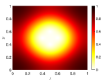
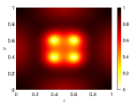
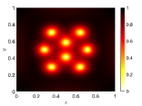
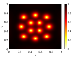
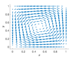
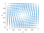
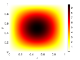
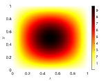
and the particular values for the GL parameter $\kappa=6,12,18,24$. We compute the discrete minimizers with the LOD approximation for the order parameter $u$ and quadratic FE for the vector potential $\mathbf{A}$ with the iterative solver described in Section 7.1. We choose the mesh sizes $H=2^{-7}$ and $h=2^{-9}$ and compute the minimizers up to a tolerance of $\varepsilon_{\mathrm{tol}}=10^{-10}$ with the step size $\tau=1$. For the practical realization of the LOD spaces we solve the corrector problems from (3.4) with $\mathcal{P}_{1}$-Lagrange FE on a fine mesh with mesh size $h_{\mathrm{fine}}=2^{-9}$ and with a localization to $\ell=10$ oversampling layers; see [BDH24] for details. The computed discrete minimizers are shown in Figure 1 and the corresponding energy values are given in Table 1. These solutions serve as reference solutions for the subsequent experiments and are for convenience again denoted by $(u,\mathbf{A})$.

Refer to caption
Refer to caption
Refer to caption
Refer to caption
Refer to caption
Refer to caption
Refer to caption
Refer to caption
Refer to caption
Refer to caption
Refer to caption
Refer to caption
Figure 1. Minimizers $(u,\mathbf{A})$ for $\kappa=6,12,18,24$ (left to right) computed with the LOD approximation in the order parameter $u$ and quadratic FE for the vector potential $\mathbf{A}$. Top row: order parameter $|u|$. Middle row: vector potential $\mathbf{A}$ (plotted on a coarse mesh). Bottom row: $\operatorname{curl}\mathbf{A}$ of the vector potential.
$\kappa$ 6 12 18 24
$E_{\mbox{\tiny GL}}(u,\mathbf{A})$ 0.393563 0.271846 0.208339 0.182871
Table 1. Approximate energy $E_{\mbox{\tiny GL}}(u,\mathbf{A})$ of the minimizers for $\kappa=6,12,18,24$.

In the order parameter $u$ (Figure 1, top row) we see the expected vortex patterns, known as the Abrikosov lattice, that occur in type-II superconductors penetrated by external magnetic fields. The vortices are well resolved by the LOD approximation space, consistent with the observations of [BDH24] for the reduced Ginzburg–Landau model with given vector potentials $\mathbf{A}$. The number of vortices increases and their diameter decreases while the GL parameter $\kappa$ increases. Looking at the vector potential $\mathbf{A}$ (Figure 1, middle line), we clearly see that no special vortex-like structure appears in the vector potential. This justifies the choice of a standard FE discretization for the vector potential $\mathbf{A}$. The physically relevant observable is $\operatorname{curl}\mathbf{A}$, shown in the bottom row of Figure 1, which describes the magnetic field inside the superconductor. As expected, it is aligned with the external magnetic field $\mathbf{H}$. Furthermore, we observed during the computation that the alignment stabilizes after a few iterations, so our strategy for updating the LOD space is empirically justified. The challenging variable is the order parameter as we have seen that it takes a lot of iterations until the right vortex-pattern appears and the gradient flow converges.

Refer to caption
Refer to caption
Figure 2. Error of the order parameter $u$ for the mesh sizes $H=2^{-\{2,3,4,5,6\}}$, $h=2^{-7}$ and LOD parameters $h_{\mathrm{fine}}=2^{-9}$ and $\ell=10$. Left: $\kappa$-scaled $H^{1}_{\kappa}$-error $\kappa^{-3}\|u-u^{{\mbox{\tiny LOD}}}_{H}\|_{H^{1}_{\kappa}}$. Right: $\kappa$-scaled $L^{2}$-error $\kappa^{-4}\|u-u^{{\mbox{\tiny LOD}}}_{H}\|_{L^{2}}$

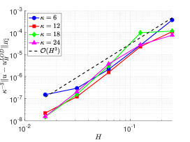
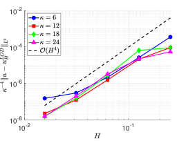
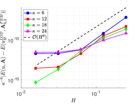
Next we investigate the error of the approximations of the minimizers and its dependence on the mesh sizes $H,h$ and on the GL parameter $\kappa$ as stated in Theorem 3.2. For the first experiment, we choose a fixed fine mesh size $h=2^{-7}$ for the vector potential $\mathbf{A}$, different mesh sizes $H=2^{-\{2,3,4,5,6\}}$ for the LOD approximation in the order parameter $u$, and compute the errors $\|u-u_{H}^{\mbox{\tiny LOD}}\|_{H^{1}_{\kappa}}$ and $\|u-u_{H}^{\mbox{\tiny LOD}}\|_{L^{2}}$ to the reference solution for the different values $\kappa=6,12,18,24$. All other parameters are chosen as for the reference solutions above. Due to the fine mesh size in the vector potential we can expect that the overall error $(u-u_{H}^{{\mbox{\tiny LOD}}},\mathbf{A}-\mathbf{A}_{h,2}^{\mbox{\tiny FEM}})$ is dominated by the error in the order parameter. The results are depicted in Figure 2. We observe after a short pre-asymptotic phase an order three decay of the $H^{1}_{\kappa}$-error w.r.t. the mesh size and an order four decay of the $L^{2}$-error w.r.t. the mesh size. The pre-asymptotic phase is explained by the resolution condition $H\lesssim C_{\textup{sol}}(u,\mathbf{A},\kappa)^{-1/4}\kappa^{-1}$ that we previously discussed in Section 3.1 after Theorem 3.2. For $H=2^{-6}$ both the errors start to stagnate which is most-likely due to the fine scale discretization of order $\mathcal{O}(h_{\mathrm{fine}})$ that we used to solve the local corrector problems for the LOD space. This behavior was also observed in [BDH24] and we refer to it for a more detailed discussion. Let us now turn to the $\kappa$-dependence of the error. We point out that in Figure 2 the $H^{1}_{\kappa}$-error is scaled with a $\kappa^{-3}$ pre-factor and the $L^{2}$-error with a $\kappa^{-4}$ pre-factor respectively. We observe that the error curves are almost on top of each other as $\kappa$ varies and emphasize that a different $\kappa$-scaling of the error leads to a significant difference between the error curves. Therefore, we conclude that the $\kappa^{3}$-dependence (resp. $\kappa^{4}$-dependence) of the $H^{1}_{\kappa}$-error (resp. $L^{2}$-error) in our theoretical convergence result is optimal. Summarizing, the numerical experiments verifies the $\mathcal{O}(\kappa^{3}H^{3})$ (resp. $\mathcal{O}(\kappa^{4}H^{4})$) decay of the $H^{1}_{\kappa}$-error (resp. $L^{2}$-error) in the order parameter $u$ as proved in Theorem 3.2.

Refer to caption
Refer to caption
Figure 3. Error of the vector potential $\mathbf{A}$ for the mesh sizes $h=2^{-\{2,3,4,5,6,7\}}$, $H=2^{-5}$ and LOD parameters $h_{\mathrm{fine}}=2^{-9}$ and $\ell=10$. Left: $\mathbf{H}^{1}$-error $\|\mathbf{A}-\mathbf{A}_{h,2}^{\mbox{\tiny FEM}}\|_{\mathbf{H}^{1}}$. Right: $\mathbf{L}^{2}$-error $\|\mathbf{A}-\mathbf{A}_{h,2}^{\mbox{\tiny FEM}}\|_{\mathbf{L}^{2}}$.

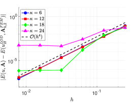
In the next experiment we extract the convergence in the vector potential $\mathbf{A}$. We fix a small mesh size $H=2^{-5}$ for the order parameter, vary the mesh size $h=2^{-\{2,3,4,5,6,7\}}$ for the vector potential, and compute the errors $\|\mathbf{A}-\mathbf{A}_{h,2}^{\mbox{\tiny FEM}}\|_{\mathbf{H}^{1}}$ and $\|\mathbf{A}-\mathbf{A}_{h,2}^{\mbox{\tiny FEM}}\|_{\mathbf{L}^{2}}$. Again all other parameters are set as before and we can now expect that the overall error is dominated by the error in the vector potential $\mathbf{A}$. The results are shown in Figure 3 where we can see that the $\mathbf{H}^{1}$-error decays in a clear asymptotic phase with a rate of two w.r.t. $h$ after a short pre-asymptotic phase for the larger values $\kappa=18$ and $\kappa=24$. The pre-asymptotic phase is now explained by the resolution condition $h\lesssim C_{\textup{sol}}(u,\mathbf{A},\kappa)^{-1/3}\kappa^{-1/3}$. This coincides with our theoretical findings from Theorem 3.2. But, in view of the $\kappa$-dependence, we see that the convergence curves are almost exactly on top of each other, although we did not include any $\kappa$-scaling of the $\mathbf{H}^{1}$-error. This clearly indicates that our error estimates of order $\mathcal{O}(\kappa h^{2})$ might be suboptimal w.r.t. $\kappa$ as an implication of a possibly suboptimal estimate of $\|\mathbf{A}\|_{\mathbf{H}^{3}}$ in the analysis; see Remark 3.3 for a more detailed discussion. For the $\mathbf{L}^{2}$-error we also observe a clear third order convergence rate w.r.t. the mesh size in the asymptotic phase, i.e., for small values of $h$ and small values of $\kappa=6,12,18$. The curves for $\kappa=18$ and $\kappa=24$ show a significant pre-asymptotic regime from $h=2^{-2}$ to $h=2^{-3}$ as for the $\mathbf{H}^{1}$ error, but it is too small to allow for any further conclusions about its $\kappa$-dependence. The curve for $\kappa=24$ shows an unstable third order convergence for $h^{-3}$ to $h^{-7}$, which indicates pollution by further pre-asymptotic effects, but again does not allow for any reliable conclusions. Nevertheless, as for the $\mathbf{H}^{1}$-error, we see no $\kappa$-dependence of the $\mathbf{L}^{2}$-error (apart from the $\kappa=24$ curve) which again points to suboptimality of our estimates in the $\kappa$-scaling. Besides this, the experiment confirms our theoretical results w.r.t. the vector potential.

Refer to caption
Refer to caption
Figure 4. Error of the energy $E$ with LOD parameters $h_{\mathrm{fine}}=2^{-9}$ and $\ell=10$. Left: $\kappa^{-6}|E(u,\mathbf{A})-E(u^{{\mbox{\tiny LOD}}}_{H},\mathbf{A}_{h,2}^{\mbox{\tiny FEM}})|$ for the mesh sizes $H=2^{-\{2,3,4,5,6\}}$, $h=2^{-7}$. Right: $|E(u,\mathbf{A})-E(u^{{\mbox{\tiny LOD}}}_{H},\mathbf{A}_{h,2}^{\mbox{\tiny FEM}})|$ for the mesh sizes $h=2^{-\{2,3,4,5,6,7\}}$, $H=2^{-5}$.

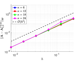
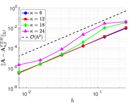
In both experiments we additionally computed the error in the Ginzburg–Landau energy which are shown in Figure 4. The error in energy takes the convergence in both components into account and we see in both error plots a convergence in three phases: a pre-asymptotic phase, an asymptotic phase, and a stagnation phase. The occurrence of the pre-asymptotic phase is again caused by the resolution conditions discussed above. The stagnation of the error is due to the fixed mesh size $h$ for the vector potential (Figure 4 left) or the fixed mesh size $H$ for the order parameter (Figure 4 right). In the asymptotic phase the errors show the predicted sixth order convergence w.r.t. $H$ and correct $\kappa^{-6}$-scaling in Figure 4 left. In Figure 4 right we observe the expected fourth order convergence w.r.t. $h$ but again no $\kappa$-scaling. Except for the latter, this is again in agreement with our main results.

Acknowledgment

The authors would like to thank Wolfgang Reichel and Roland Schnaubelt for valuable discussions on the elliptic regularity.

Statements and Declarations

The authors declare that they have no financial or non-financial competing interests directly or indirectly related to the work.

References

Appendix A Proofs of the higher regularity results

In this section, we collect the proofs of Theorem 2.6 and Lemma 2.8. As we could not find any suitable reference which covers our cases, we present the proofs here in the appendix, even though these results might be known to many experts.

For the sake of notation, we restrict ourselves to the unit cube $\Omega=(0,1)^{3}$, but the case of general cuboids is easily derived by a linear transformation. For $\widehat{\Omega}_{s}=(-s,s)^{3}$, $s\in\mathbb{R}^{+}$, the idea is to use reflections to extend the functions from $\Omega$ to the extended domain $\widehat{\Omega}_{1}$, and then periodically to any $\widehat{\Omega}_{2k+1}$ for $k\in\mathbb{N}$ while preserving its regularity.

The main intuition for this procedure comes from the eigenbasis of the Laplacian on a cube. For example, for homogeneous Dirichlet boundary conditions the basis on $\Omega$ consists of functions

(A.1) $$\sin(\pi kx_{1})\sin(\pi\ell x_{2})\sin(\pi mx_{3}),\quad k,\ell,m\geq 1,$$

and their natural extension is given by first performing an odd reflection on each face and then obtain a periodic function on $\widehat{\Omega}_{1}$. For Neumann boundary conditions, the same idea applies with the basis

(A.2) $$\cos(\pi kx_{1})\cos(\pi\ell x_{2})\cos(\pi mx_{3}),\quad k,\ell,m\geq 0,$$

and hence even reflections on each face. For mixed problems the correct combination of sine and cosine enable us to extend this also to the mixed case.

A.1. Neumann boundary conditions

Let us consider the Neumann problem in Lemma 2.8 given by

(A.3) $$-\Delta u=g\mbox{ in }\Omega\qquad\mbox{and}\qquad\nabla u\cdot\nu|_{\partial\Omega}=0,$$

for $g\in L^{2}(\Omega)$. For a function $f\in C(\bar{\Omega})$, we define the Neumann extension $M_{N}\colon f\to f_{\mbox{\tiny ext}}$ with

(A.4) $\displaystyle f_{\mbox{\tiny ext}}(x_{1},x_{2},x_{3})=\begin{cases}f(x_{1},x_{2},x_{3}),\,&x_{1}\in(0,1),x_{2}\in(0,1),x_{3}\in(0,1),\\ f(x_{1},x_{2},-x_{3}),\quad&x_{1}\in(0,1),x_{2}\in(0,1),x_{3}\in(-1,0),\\ f(x_{1},-x_{2},-x_{3}),\quad&x_{1}\in(0,1),x_{2}\in(-1,0),x_{3}\in(-1,0),\\ f(x_{1},-x_{2},x_{3}),\quad&x_{1}\in(0,1),x_{2}\in(-1,0),x_{3}\in(0,1),\\ f(-x_{1},x_{2},x_{3}),\quad&x_{1}\in(-1,0),x_{2}\in(0,1),x_{3}\in(0,1),\\ f(-x_{1},x_{2},-x_{3}),\quad&x_{1}\in(-1,0),x_{2}\in(0,1),x_{3}\in(-1,0),\\ f(-x_{1},-x_{2},-x_{3}),\quad&x_{1}\in(-1,0),x_{2}\in(-1,0),x_{3}\in(-1,0),\\ f(-x_{1},-x_{2},x_{3}),\quad&x_{1}\in(-1,0),x_{2}\in(-1,0),x_{3}\in(0,1).\end{cases}$

Without changing the notation, we extend the operator $M_{N}$ also to $L^{2}$-functions.

Lemma A.1.

Let $f\in H^{1}(\Omega)$. Then the extension $M_{N}f$ satisfies:

(a) $M_{N}f\in H^{1}(\widehat{\Omega}_{1})$ with $\lvert|M_{N}f\rvert|_{H^{1}(\widehat{\Omega}_{1})}\leq 2^{3}\lvert|M_{N}f\rvert|_{H^{1}(\Omega)}$.

(b) The periodic extension of $M_{N}f$ satisfies $M_{N}f\in H^{1}(\widehat{\Omega}_{2k+1})$ for all $k\geq 1$ with

(A.5) $$\lvert|M_{N}f\rvert|_{H^{1}(\widehat{\Omega}_{2k+1})}\leq(2k+2)^{3}\lvert|M_{N}f\rvert|_{H^{1}(\Omega)}.$$
Proof.

(a) Since $M_{N}f$ is in $H^{1}$ on each subdomain, it remains to check that the trace is continuous in the $L^{2}$ sense on the faces. However, the even reflection ensures this continuity. Since the $H^{1}$-norm on each subdomain is equal to the $H^{1}$-norm on $\Omega$, the estimate in (a) follows by counting cubes.

(b) For the periodic case, it is sufficient to note that the periodic extension from $\widehat{\Omega}_{1}$ is equivalent to iteratively performing even reflections on the outer faces. In particular, this implies continuity at all outer faces of $\widehat{\Omega}_{1}$, by repeating the calculation of the interior faces. ∎

We now turn to the case of preserving $H^{2}$-regularity.

Lemma A.2.

Let $f\in H^{2}(\Omega)$ with $\nabla f\cdot\nu|_{\partial\Omega}=0$. Then the extension $M_{N}f$ satisfies:

(a) $M_{N}f\in H^{2}(\widehat{\Omega}_{1})$ with $\lvert|M_{N}f\rvert|_{H^{2}(\widehat{\Omega}_{1})}\leq 2^{3}\lvert|M_{N}f\rvert|_{H^{2}(\Omega)}$.

(b) The periodic extension of $M_{N}f$ satisfies $M_{N}f\in H^{2}(\widehat{\Omega}_{2k+1})$ for all $k\geq 1$ with

(A.6) $$\lvert|M_{N}f\rvert|_{H^{2}(\widehat{\Omega}_{2k+1})}\leq(2k+2)^{3}\lvert|M_{N}f\rvert|_{H^{2}(\Omega)}.$$
Proof.

We note that it is sufficient to show that $\Delta f_{\mbox{\tiny ext}}\in L^{2}(\widehat{\Omega}_{1})$ and elliptic regularity gives us the claim. We further note, that the periodic extension is handled as in Lemma A.1.

Since we already know that $M_{N}f\in H^{2}$ on each subdomain and $M_{N}f\in H^{1}(\widehat{\Omega}_{1})$, in order to show that $\nabla f_{\mbox{\tiny ext}}\in H(\operatorname{div},\widehat{\Omega}_{1})$ holds, we have to prove that all normal traces of $\nabla f_{\mbox{\tiny ext}}$ are continuous.

Computing the gradients on each subdomain, we obtain for the diagonal matrix $I_{a,b,c}=\operatorname{diag}(a,b,c)$ the expressions

(A.7) $\displaystyle\nabla f_{\mbox{\tiny ext}}(x_{1},x_{2},x_{3})=\begin{cases}I_{1,1,1}\nabla f\big{|}_{(x_{1},x_{2},x_{3})},\quad&x_{1}\in(0,1),x_{2}\in(0,1),x_{3}\in(0,1),\\ I_{1,1,-1}\nabla f\big{|}_{(x_{1},x_{2},-x_{3})},\quad&x_{1}\in(0,1),x_{2}\in(0,1),x_{3}\in(-1,0),\\ I_{1,-1,-1}\nabla f\big{|}_{(x_{1},-x_{2},-x_{3})},\quad&x_{1}\in(0,1),x_{2}\in(-1,0),x_{3}\in(-1,0),\\ I_{1,-1,1}\nabla f\big{|}_{(x_{1},-x_{2},x_{3})},\quad&x_{1}\in(0,1),x_{2}\in(-1,0),x_{3}\in(0,1),\\ I_{-1,1,1}\nabla f\big{|}_{(-x_{1},x_{2},x_{3})},\quad&x_{1}\in(-1,0),x_{2}\in(0,1),x_{3}\in(0,1),\\ I_{-1,1,-1}\nabla f\big{|}_{(-x_{1},x_{2},-x_{3})},\quad&x_{1}\in(-1,0),x_{2}\in(0,1),x_{3}\in(-1,0),\\ I_{-1,-1,-1}\nabla f\big{|}_{(-x_{1},-x_{2},-x_{3})},\quad&x_{1}\in(-1,0),x_{2}\in(-1,0),x_{3}\in(-1,0),\\ I_{-1,-1,1}\nabla f\big{|}_{(-x_{1},-x_{2},x_{3})},\quad&x_{1}\in(-1,0),x_{2}\in(-1,0),x_{3}\in(0,1).\end{cases}$

We only check the face $\{x_{1}=0,x_{2}\in(0,1),x_{3}\in(0,1)\}$ with normal vector $\nu=e_{1}$ to obtain formally for all $x_{2}\in(0,1),x_{3}\in(0,1)$

(A.8) $\displaystyle\lim\limits_{x_{1}\to 0^{+}}\partial_{\nu}f_{\mbox{\tiny ext}}(x_{1},x_{2},x_{3})=\lim\limits_{x_{1}\to 0^{+}}\partial_{1}f(x_{1},x_{2},x_{3})=\partial_{1}f(0,x_{2},x_{3})=0$

as well as

(A.9) $\displaystyle\lim\limits_{x_{1}\to 0^{-}}\partial_{\nu}f_{\mbox{\tiny ext}}(x_{1},x_{2},x_{3})=\lim\limits_{x_{1}\to 0^{+}}-\partial_{1}f(-x_{1},x_{2},x_{3})=-\partial_{1}f(0,x_{2},x_{3})=0.$

For the other faces the very same computations can be performed. Thus, all normal traces of $\nabla f_{\mbox{\tiny ext}}$ vanish on the inner faces, are thus in particular continuous, and we have shown $\nabla f_{\mbox{\tiny ext}}\in H(\operatorname{div},\widehat{\Omega}_{1})$. ∎

With this, we are in the position to prove Lemma 2.8.

Proof of Lemma 2.8.

First, we observe with Lemmas A.1 and A.2 that for $u_{\mbox{\tiny ext}}=M_{N}u$

(A.10) $$-\Delta u_{\mbox{\tiny ext}}\big{|}_{(x_{1},x_{2},x_{3})}=-\Delta u\big{|}_{(\pm x_{1},\pm x_{2},\pm x_{3})}=f\big{|}_{(\pm x_{1},\pm x_{2},\pm x_{3})}=f_{\mbox{\tiny ext}}(x_{1},x_{2},x_{3}),$$

with signs chosen accordingly to the definition of $M_{N}$. In particular, $u_{\mbox{\tiny ext}}$ solves the Neumann problem in Lemma 2.8 also on $\widehat{\Omega}_{3}$ with right-hand side $f_{\mbox{\tiny ext}}\in H^{1}(\widehat{\Omega}_{3})$. By interior regularity for elliptic problems (cf. [Evans10, Theorem 6.3.2]) we conclude $u=u_{\mbox{\tiny ext}}|_{\Omega}\in H^{3}(\Omega)$ with

$\displaystyle\|u\|_{H^{3}(\Omega)}$ $\displaystyle\lesssim$ $\displaystyle\|u_{\mbox{\tiny ext}}\|_{L^{2}(\widehat{\Omega}_{3})}+\|f_{\mbox{\tiny ext}}\|_{H^{1}(\widehat{\Omega}_{3})}\,\,\,\lesssim\,\,\,\|u\|_{L^{2}(\Omega)}+\|f\|_{H^{1}(\Omega)}.$

Next, we turn towards the $W^{2,p}$-regularity of $u$, where we exploit again the extensions $u_{\mbox{\tiny ext}}$ and $f_{\mbox{\tiny ext}}$ together with a Calderón–Zygmund estimate. For that, let $B_{\mbox{\tiny ext}}$ be a ball with radius $r=2$, which is compactly contained in the extended domain $\widehat{\Omega}_{3}$. In particular, we have $\Omega\subset\subset B_{\mbox{\tiny ext}}\subset\subset\widehat{\Omega}_{3}$ and a regular boundary $\partial B_{\mbox{\tiny ext}}\in C^{1,1}$. We want to smoothly truncate $u_{\mbox{\tiny ext}}$ to $B_{\mbox{\tiny ext}}$ with a cut-off function $\eta\in C^{\infty}_{0}(B_{\mbox{\tiny ext}})$ with $0\leq\eta\leq 1$. Furthermore, $\eta$ should not only be constant $1$ on $\Omega$, but also on a slightly enlarged box, that is, $\eta\equiv 1$ on $\widehat{\Omega}_{1+\delta}$ for a sufficiently small $\delta$ such that we still have $\widehat{\Omega}_{1+\delta}\subset\subset B_{\mbox{\tiny ext}}$. Finally, assume that $\eta$ is selected such that $\|\nabla\eta\|_{L^{\infty}}\leq C$ for some constant $C$ that only depends on $B_{\mbox{\tiny ext}}$ and $\widehat{\Omega}_{3}$. We consider the function $\eta\,u_{\mbox{\tiny ext}}\in H^{1}_{0}(B_{\mbox{\tiny ext}})$ which solves

$$-\Delta(\eta\,u_{\mbox{\tiny ext}})=-\eta\,\Delta u_{\mbox{\tiny ext}}-2\nabla u_{\mbox{\tiny ext}}\cdot\nabla\eta-u_{\mbox{\tiny ext}}\,\Delta\eta=\eta\,f_{\mbox{\tiny ext}}-2\nabla u_{\mbox{\tiny ext}}\cdot\nabla\eta-u_{\mbox{\tiny ext}}\,\Delta\eta=:\tilde{f}_{\mbox{\tiny ext}}.$$

Since $u_{\mbox{\tiny ext}}\in H^{3}(B_{\mbox{\tiny ext}})$ (by interior regularity from the first part of the proof), Sobolev embeddings guarantee that we also have $\nabla u_{\mbox{\tiny ext}}\in L^{\infty}(B_{\mbox{\tiny ext}})$. Together with $f_{\mbox{\tiny ext}}\in L^{p}(B_{\mbox{\tiny ext}})$ (which directly follows from $f\in L^{p}(\Omega)$), we conclude that $\eta\,u_{\mbox{\tiny ext}}\in H^{1}_{0}(B_{\mbox{\tiny ext}})$ is the unique solution to a Poisson problem on a smooth domain $B_{\mbox{\tiny ext}}$, with homogeneous Dirichlet boundary condition and a right-hand side $\tilde{f}_{\mbox{\tiny ext}}\in L^{p}$. By $L^{p}$-regularity theory for elliptic problems, cf. [ChenWuEllipticTheoryLp, Chapt. 3, Thm. 6.3 & Thm. 6.4], we conclude that this unique solution fulfills $\eta\,u_{\mbox{\tiny ext}}\in W^{2,p}(B_{\mbox{\tiny ext}})$. By construction of the cut-off function, we have $u_{\mbox{\tiny ext}}|_{\widehat{\Omega}_{1+\delta}}=(\eta\,u_{\mbox{\tiny ext}})|_{\widehat{\Omega}_{1+\delta}}\in W^{2,p}(\widehat{\Omega}_{1+\delta})$. Furthermore, we still have $-\Delta u_{\mbox{\tiny ext}}=f_{\mbox{\tiny ext}}$ in $\widehat{\Omega}_{1+\delta}\subset\widehat{\Omega}_{3}$. Using the Calderón–Zygmund estimate [GiT01, Theorem 9.11] with $\Omega\subset\subset\widehat{\Omega}_{1+\delta}$, we conclude that there exist constants (depending on $p$, $\Omega$ and $\delta$), such that

(A.11) $\displaystyle\|u\|_{W^{2,p}(\Omega)}=\|u_{\mbox{\tiny ext}}\|_{W^{2,p}(\Omega)}\lesssim\bigl{(}\|u_{\mbox{\tiny ext}}\|_{L^{p}(\widehat{\Omega}_{1+\delta})}+\|f_{\mbox{\tiny ext}}\|_{L^{p}(\widehat{\Omega}_{1+\delta})}\bigr{)}\lesssim\bigl{(}\|u\|_{L^{p}(\Omega)}+\|f\|_{L^{p}(\Omega)}\bigr{)},$

which proves the claim. ∎

A.2. Mixed boundary conditions

We now turn to the regularity results of the vector potential $\mathbf{A}$. As mentioned above, the $H^{2}$-regularity of a solution $\mathbf{U}\in\mathbf{H}^{1}_{\mathrm{n},\operatorname{div}}(\Omega)$ of (2.17) follows from [HocJS15, Lemma 3.7]. In addition, the reference shows that the first component $\mathbf{U}_{1}$ satisfies

(A.12) $\displaystyle-\Delta\mathbf{U}_{1}$ $\displaystyle=f\text{ in }\Omega,$
$\displaystyle\mathbf{U}_{1}$ $\displaystyle=0\text{ on }\Gamma_{1}=\{x\in\Omega\mid x_{1}=0\text{ or }x_{1}=1\},$
$\displaystyle\partial_{2}\mathbf{U}_{1}$ $\displaystyle=0\text{ on }\Gamma_{2}=\{x\in\Omega\mid x_{2}=0\text{ or }x_{2}=1\},$
$\displaystyle\partial_{3}\mathbf{U}_{1}$ $\displaystyle=0\text{ on }\Gamma_{3}=\{x\in\Omega\mid x_{3}=0\text{ or }x_{3}=1\},$

and similarly the other two components by interchanging the roles of the faces. We thus only study the case of $\mathbf{U}_{1}$. We follow the ideas of the Neumann case but now with the eigenbasis of the from

(A.13) $$\sin(\pi kx)\cos(\pi\ell y)\cos(\pi mz)$$

in mind. This means odd reflections in $x_{1}$-direction and even reflections on $x_{2}$- and $x_{3}$-direction. We therefore introduce the spaces

(A.14) $\displaystyle H_{0,1}^{1}(\Omega)$ $\displaystyle\coloneqq\{\varphi\in H^{1}(\Omega)\mid\varphi=0\text{ on }\Gamma_{1}\},$
(A.15) $\displaystyle H_{0,1}^{2}(\Omega)$ $\displaystyle\coloneqq\{\varphi\in H^{2}(\Omega)\mid\varphi=0\text{ on }\Gamma_{1},\,\partial_{\nu}\varphi=0\text{ on }\Gamma_{2}\cup\Gamma_{3}\}.$

If $\Omega$ is replaced by a larger cube $\widehat{\Omega}_{s}$, we denote by $\Gamma_{i}\coloneqq\{x\in\partial\widehat{\Omega}_{s}\mid x_{i}=-s\text{ or }x_{i}=s\}$. For a function $f\in C(\bar{\Omega})$, we define the mixed extension $M_{D,N}\colon f\to f_{\mbox{\tiny ext}}$ with

(A.16) $\displaystyle f_{\mbox{\tiny ext}}(x_{1},x_{2},x_{3})=\begin{cases}f(x_{1},x_{2},x_{3}),\quad&x_{1}\in(0,1),x_{2}\in(0,1),x_{3}\in(0,1),\\ f(x_{1},x_{2},-x_{3}),\quad&x_{1}\in(0,1),x_{2}\in(0,1),x_{3}\in(-1,0),\\ f(x_{1},-x_{2},-x_{3}),\quad&x_{1}\in(0,1),x_{2}\in(-1,0),x_{3}\in(-1,0),\\ f(x_{1},-x_{2},x_{3}),\quad&x_{1}\in(0,1),x_{2}\in(-1,0),x_{3}\in(0,1),\\ -f(-x_{1},x_{2},x_{3}),\quad&x_{1}\in(-1,0),x_{2}\in(0,1),x_{3}\in(0,1),\\ -f(-x_{1},x_{2},-x_{3}),\quad&x_{1}\in(-1,0),x_{2}\in(0,1),x_{3}\in(-1,0),\\ -f(-x_{1},-x_{2},-x_{3}),\quad&x_{1}\in(-1,0),x_{2}\in(-1,0),x_{3}\in(-1,0),\\ -f(-x_{1},-x_{2},x_{3}),\quad&x_{1}\in(-1,0),x_{2}\in(-1,0),x_{3}\in(0,1).\end{cases}$

As in the Neumann case, this extension preserves the regularity of the inserted functions.

Lemma A.3.

Let $f\in H_{0,1}^{1}(\Omega)$ and $g\in H_{0,1}^{2}(\Omega)$.

(a) $M_{D,N}f\in H_{0,1}^{1}(\widehat{\Omega}_{1})$ with $\lvert|M_{N}f\rvert|_{H^{1}(\widehat{\Omega}_{1})}\leq 2^{3}\lvert|M_{N}f\rvert|_{H^{1}(\Omega)}$.

(b) The periodic extension of $M_{D,N}f$ satisfies $M_{D,N}f\in H_{0,1}^{1}(\widehat{\Omega}_{2k+1})$ for all $k\geq 1$ with

(A.17) $$\lvert|M_{D,N}f\rvert|_{H^{1}(\widehat{\Omega}_{2k+1})}\leq(2k+2)^{3}\lvert|M_{D,N}f\rvert|_{H^{1}(\Omega)}.$$

(c) $M_{D,N}g\in H_{0,1}^{2}(\widehat{\Omega}_{1})$ with $\lvert|M_{D,N}g\rvert|_{H^{2}(\widehat{\Omega}_{1})}\leq 2^{3}\lvert|M_{D,N}g\rvert|_{H^{2}(\Omega)}$.

(d) The periodic extension of $M_{D,N}f$ satisfies $M_{N}g\in H_{0,1}^{2}(\widehat{\Omega}_{2k+1})$ for all $k\geq 1$ with

(A.18) $$\lvert|M_{D,N}g\rvert|_{H^{2}(\widehat{\Omega}_{2k+1})}\leq(2k+2)^{3}\lvert|M_{D,N}g\rvert|_{H^{2}(\Omega)}.$$
Proof.

The claims on $H^{1}$ are easily verified, as we preserve continuity at all faces. Further, the computations for all faces where $x_{1}$ is either positive or negative are fully analogous to Lemma A.2 as all the normal traces vanish. Hence, we check the conditions at $x_{1}=0$, and let for example $x_{2},x_{3}<0$. Then,

(A.19) $\displaystyle\nabla f_{\mbox{\tiny ext}}(x_{1},x_{2},x_{3})$ $\displaystyle=I_{1,-1,-1}\nabla f\big{|}_{(x_{1},-x_{2},-x_{3})},\quad$ $\displaystyle x_{1}>0$
(A.20) $\displaystyle\nabla f_{\mbox{\tiny ext}}(x_{1},x_{2},x_{3})$ $\displaystyle=-I_{-1,-1,-1}\nabla f\big{|}_{(-x_{1},-x_{2},-x_{3})},\quad$ $\displaystyle x_{1}<0,$

and we obtain

(A.21) $\displaystyle\lim\limits_{x_{1}\to 0^{+}}\partial_{\nu}f_{\mbox{\tiny ext}}(x_{1},x_{2},x_{3})=\lim\limits_{x_{1}\to 0^{+}}\partial_{1}f(x_{1},-x_{2},-x_{3})=\partial_{1}f(0,-x_{2},-x_{3})$

as well as

(A.22) $\displaystyle\lim\limits_{x_{1}\to 0^{-}}\partial_{\nu}f_{\mbox{\tiny ext}}(x_{1},x_{2},x_{3})=\lim\limits_{x_{1}\to 0^{+}}\partial_{1}f(-x_{1},-x_{2},-x_{3})=\partial_{1}f(0,-x_{2},-x_{3}),$

and we also obtain here the continuity of the normal traces of the gradient. ∎

We can then turn to the proof of the second part of Theorem 2.6.

Proof of Theorem 2.6 (b).

Let us recall that by part (a) $\mathbf{U}\in\mathbf{H}^{2}(\Omega)$ solves

(A.23) $$\Delta\mathbf{U}=\mathbf{G},\qquad\mathbf{U}\cdot\nu|_{\partial\Omega}=\operatorname{curl}\mathbf{U}\times\nu|_{\partial\Omega}=0,$$

with $\mathbf{G}=\mathbf{F}+\operatorname{curl}\mathbf{H}$. The regularity of $\mathbf{H}$ and $\mathbf{F}$ and the conditions

(A.24) $$\operatorname{curl}\mathbf{H}\cdot\nu|_{\partial\Omega}=\mathbf{F}\cdot\nu|_{\partial\Omega}=0\quad\text{imply }\quad\mathbf{G}\in\mathbf{H}^{1}(\Omega)\,\,\mbox{and}\,\,\mathbf{G}\cdot\nu|_{\partial\Omega}=0.$$

Now taking the first component $\mathbf{U}_{1}$, wee see that $f$ in (A.12) is given by the first component of $\mathbf{G}$, and thus satisfies $f\in H^{1}_{0,1}(\Omega)$. Lemma A.3 further ensures that $f_{\mbox{\tiny ext}}\in H^{1}_{0,1}(\widehat{\Omega}_{3})$ holds. For $\mathbf{U}_{\mbox{\tiny ext}}=M_{D,N}\mathbf{U}$ we argue as in the proof of Lemma 2.8 and observe that choosing the correct case in the definition of $M_{D,N}$

(A.25) $$-\Delta\mathbf{U}_{\mbox{\tiny ext}}\big{|}_{(x_{1},x_{2},x_{3})}=(-1)^{m}\Delta\mathbf{U}\big{|}_{(\pm x_{1},\pm x_{2},\pm x_{3})}=(-1)^{m}f\big{|}_{(\pm x_{1},\pm x_{2},\pm x_{3})}=f_{\mbox{\tiny ext}}(x_{1},x_{2},x_{3})$$

with $m=0$ for $x_{1}>0$ and $m=1$ for $x_{1}<0$. Hence, $\mathbf{U}_{\mbox{\tiny ext}}\in H^{2}_{0,1}(\widehat{\Omega}_{3})$ solves the mixed problem (A.12) with right-hand side $f_{\mbox{\tiny ext}}\in H^{1}_{0,1}(\widehat{\Omega}_{3})$. Again, interior regularity for elliptic problems (cf. [Evans10, Theorem 6.3.2]) gives $\mathbf{U}=\mathbf{U}_{\mbox{\tiny ext}}|_{\Omega}\in H^{3}(\Omega)$ with

(A.26) $\displaystyle\|\mathbf{U}\|_{H^{3}(\Omega)}\lesssim\|\mathbf{U}_{\mbox{\tiny ext}}\|_{L^{2}(\widehat{\Omega}_{3})}+\|f_{\mbox{\tiny ext}}\|_{H^{1}(\widehat{\Omega}_{3})}\lesssim\|\mathbf{U}\|_{L^{2}(\Omega)}+\|f\|_{H^{1}(\Omega)},$

which yields the claim. ∎

Appendix B Proofs of additional auxiliary results

In this section, we present the proofs of Lemma 5.5 and Lemma 6.1.

Proof of Lemma 5.5.

Using $\partial_{u}E(u,\mathbf{A})\varphi=0$ and $\partial_{\mathbf{A}}E(u,\mathbf{A})\mathbf{B}=0$, we obtain the identity

(B.1) $\displaystyle\langle E^{\prime\prime}(u,\mathbf{A})(u,\mathbf{A}),(\psi_{H},\mathbf{C}_{h})\rangle$
$\displaystyle=$ $\displaystyle\operatorname{Re}\int_{\Omega}\bigl{(}\frac{\mathrm{i}}{\kappa}\nabla u+\mathbf{A}u\bigr{)}\cdot\bigl{(}\frac{\mathrm{i}}{\kappa}\nabla\psi_{H}+\mathbf{A}\psi_{H}\bigr{)}^{*}+\bigl{(}|u|^{2}-1\bigr{)}u\psi_{H}^{*}+2|u|^{2}u\psi_{H}^{*}\,\textup{d}x$
$\displaystyle+\,\,\int_{\Omega}2|u|^{2}\mathbf{A}\cdot\mathbf{C}_{h}+\frac{1}{\kappa}\operatorname{Re}\bigl{(}\mathrm{i}u^{*}\nabla u+\mathrm{i}u^{*}\nabla u\bigr{)}\cdot\mathbf{C}_{h}\,\textup{d}x$
$\displaystyle+\,\,\int_{\Omega}2\operatorname{Re}(u\psi_{H}^{*})|\mathbf{A}|^{2}+\frac{1}{\kappa}\operatorname{Re}\bigl{(}\mathrm{i}u^{*}\nabla\psi_{H}+\mathrm{i}\psi_{H}^{*}\nabla u\bigr{)}\cdot\mathbf{A}\,\textup{d}x$
$\displaystyle+\,\,\int_{\Omega}|u|^{2}\mathbf{C}_{h}\cdot\mathbf{A}+\operatorname{curl}\mathbf{C}_{h}\cdot\operatorname{curl}\mathbf{A}+\operatorname{div}\mathbf{C}_{h}\cdot\operatorname{div}\mathbf{A}\,\textup{d}x$
$\displaystyle=$ $\displaystyle\operatorname{Re}\int_{\Omega}2|u|^{2}u\psi_{H}^{*}\,\textup{d}x\,\,+\,\,\int_{\Omega}2|u|^{2}\mathbf{A}\cdot\mathbf{C}_{h}+\frac{1}{\kappa}\operatorname{Re}\bigl{(}\mathrm{i}u^{*}\nabla u\bigr{)}\cdot\mathbf{C}_{h}\,\textup{d}x$
$\displaystyle+\,\,\int_{\Omega}2\operatorname{Re}(u\psi_{H}^{*})|\mathbf{A}|^{2}+\frac{1}{\kappa}\operatorname{Re}\bigl{(}\mathrm{i}u^{*}\nabla\psi_{H}+\mathrm{i}\psi_{H}^{*}\nabla u\bigr{)}\cdot\mathbf{A}+\mathbf{H}\cdot\operatorname{curl}\mathbf{C}_{h}\,\textup{d}x.$

Analogously, the same identity holds for $\langle E^{\prime\prime}(u_{H},\mathbf{A}_{h})(u_{H},\mathbf{A}_{h}),(\psi_{H},\mathbf{C}_{h})\rangle$ if we replace $(u,\mathbf{A})$ by $(u_{H},\mathbf{A}_{h})$ at all occurrences. Next, we use the decomposition

$\displaystyle\varepsilon_{2}$ $\displaystyle=$ $\displaystyle\underbrace{E^{\prime\prime}(u,\mathbf{A})(u,\mathbf{A})-E^{\prime\prime}(u_{H},\mathbf{A}_{h})(u_{H},\mathbf{A}_{h})}_{=:\varepsilon_{2,1}}\,\,+\,\,\underbrace{E^{\prime\prime}(u_{H},\mathbf{A}_{h})(u_{H},\mathbf{A}_{h})-E^{\prime\prime}(u,\mathbf{A})(u_{H},\mathbf{A}_{h})}_{=:\varepsilon_{2,2}}$

to sort the terms and treat them together. For the first term we obtain with (B.1) that

$\displaystyle\varepsilon_{2,1}(\psi_{H},\mathbf{C}_{h})\,\,\,=\,\,\,\underbrace{\operatorname{Re}\int_{\Omega}2(|u|^{2}u-|u_{H}|^{2}u_{H})\psi_{H}^{*}\,\textup{d}x}_{=:\alpha_{1}}\,\,+\,\,\underbrace{\int_{\Omega}2(|u|^{2}\mathbf{A}-|u_{H}|^{2}\mathbf{A}_{h})\cdot\mathbf{C}_{h}\,\textup{d}x}_{=:\alpha_{2}}$
$\displaystyle+\underbrace{\int_{\Omega}\frac{1}{\kappa}\operatorname{Re}\bigl{(}\mathrm{i}u^{*}\nabla u-\mathrm{i}u_{H}^{*}\nabla u_{H}\bigr{)}\cdot\mathbf{C}_{h}\,\textup{d}x}_{=:\alpha_{3}}\,\,+\,\,\underbrace{\int_{\Omega}2\operatorname{Re}(u\psi_{H}^{*})|\mathbf{A}|^{2}-2\operatorname{Re}(u_{H}\psi_{H}^{*})|\mathbf{A}_{h}|^{2}\,\textup{d}x}_{=:\alpha_{4}}$
$\displaystyle+\underbrace{\int_{\Omega}\frac{1}{\kappa}\operatorname{Re}\bigl{(}\mathrm{i}u^{*}\nabla\psi_{H}+\mathrm{i}\psi_{H}^{*}\nabla u\bigr{)}\cdot\mathbf{A}-\frac{1}{\kappa}\operatorname{Re}\bigl{(}\mathrm{i}u_{H}^{*}\nabla\psi_{H}+\mathrm{i}\psi_{H}^{*}\nabla u_{H}\bigr{)}\cdot\mathbf{A}_{h}\,\textup{d}x}_{=:\alpha_{5}}.$

Using

(B.2) $\displaystyle\operatorname{Re}\int_{\Omega}\bigl{(}\frac{\mathrm{i}}{\kappa}\nabla u_{H}+\mathbf{A}_{h}u_{H}\bigr{)}\cdot\bigl{(}\frac{\mathrm{i}}{\kappa}\nabla\psi_{H}+\mathbf{A}_{h}\psi_{H}\bigr{)}^{*}-\bigl{(}\frac{\mathrm{i}}{\kappa}\nabla u_{H}+\mathbf{A}u_{H}\bigr{)}\cdot\bigl{(}\frac{\mathrm{i}}{\kappa}\nabla\psi_{H}+\mathbf{A}\psi_{H}\bigr{)}^{*}\,\textup{d}x$
$\displaystyle=$ $\displaystyle\operatorname{Re}\int_{\Omega}\ \tfrac{\mathrm{i}}{\kappa}\nabla u_{H}\cdot(\mathbf{A}_{h}-\mathbf{A})\psi_{H}^{*}-\tfrac{\mathrm{i}}{\kappa}u_{H}\,(\mathbf{A}_{h}-\mathbf{A})\nabla\psi_{H}^{*}+(|\mathbf{A}_{h}|^{2}-|\mathbf{A}|^{2})u_{H}\psi_{H}^{*}\,\textup{d}x,$

the second term satisfies

$\displaystyle\varepsilon_{2,2}(\psi_{H},\mathbf{C}_{h})\,\,=\,\,\langle E^{\prime\prime}(u_{H},\mathbf{A}_{h})(u_{H},\mathbf{A}_{h}),(\psi_{H},\mathbf{C}_{h})\rangle-\langle E^{\prime\prime}(u,\mathbf{A})(u_{H},\mathbf{A}_{h}),(\psi_{H},\mathbf{C}_{h})\rangle$
$\displaystyle=$ $\displaystyle\operatorname{Re}\int_{\Omega}\bigl{(}\frac{\mathrm{i}}{\kappa}\nabla u_{H}+\mathbf{A}_{h}u_{H}\bigr{)}\cdot\bigl{(}\frac{\mathrm{i}}{\kappa}\nabla\psi_{H}+\mathbf{A}_{h}\psi_{H}\bigr{)}^{*}+\bigl{(}|u_{H}|^{2}-1\bigr{)}u_{H}\psi_{H}^{*}+u_{H}^{2}u_{H}^{*}\psi_{H}^{*}+|u_{H}|^{2}u_{H}\psi_{H}^{*}\,\textup{d}x$
$\displaystyle+\,\,\int_{\Omega}2\operatorname{Re}(u_{H}u_{H}^{*})\mathbf{A}_{h}\cdot\mathbf{C}_{h}+\frac{1}{\kappa}\operatorname{Re}\bigl{(}\mathrm{i}u_{H}^{*}\nabla u_{H}+\mathrm{i}u_{H}^{*}\nabla u_{H}\bigr{)}\cdot\mathbf{C}_{h}\,\textup{d}x$
$\displaystyle+\,\,\int_{\Omega}2\operatorname{Re}(u_{H}\psi_{H}^{*})\mathbf{A}_{h}\cdot\mathbf{A}_{h}+\frac{1}{\kappa}\operatorname{Re}\bigl{(}\mathrm{i}u_{H}^{*}\nabla\psi_{H}+\mathrm{i}\psi_{H}^{*}\nabla u_{H}\bigr{)}\cdot\mathbf{A}_{h}\,\textup{d}x$
$\displaystyle+\,\,\int_{\Omega}|u_{H}|^{2}\mathbf{C}_{h}\cdot\mathbf{A}_{h}+\operatorname{curl}\mathbf{C}_{h}\cdot\operatorname{curl}\mathbf{A}_{h}+\operatorname{div}\mathbf{C}_{h}\cdot\operatorname{div}\mathbf{A}_{h}\,\textup{d}x$
$\displaystyle-\,\,\operatorname{Re}\int_{\Omega}\bigl{(}\frac{\mathrm{i}}{\kappa}\nabla u_{H}+\mathbf{A}u_{H}\bigr{)}\cdot\bigl{(}\frac{\mathrm{i}}{\kappa}\nabla\psi_{H}+\mathbf{A}\psi_{H}\bigr{)}^{*}+\bigl{(}|u|^{2}-1\bigr{)}u_{H}\psi_{H}^{*}+u^{2}u_{H}^{*}\psi_{H}^{*}+|u|^{2}u_{H}\psi_{H}^{*}\,\textup{d}x$
$\displaystyle-\,\,\int_{\Omega}2\operatorname{Re}(uu_{H}^{*})\mathbf{A}\cdot\mathbf{C}_{h}+\frac{1}{\kappa}\operatorname{Re}\bigl{(}\mathrm{i}u^{*}\nabla u_{H}+\mathrm{i}u_{H}^{*}\nabla u\bigr{)}\cdot\mathbf{C}_{h}\,\textup{d}x$
$\displaystyle-\,\,\int_{\Omega}2\operatorname{Re}(u\psi_{H}^{*})\mathbf{A}\cdot\mathbf{A}_{h}+\frac{1}{\kappa}\operatorname{Re}\bigl{(}\mathrm{i}u^{*}\nabla\psi_{H}+\mathrm{i}\psi_{H}^{*}\nabla u\bigr{)}\cdot\mathbf{A}_{h}\,\textup{d}x$
$\displaystyle-\,\,\int_{\Omega}|u|^{2}\mathbf{C}_{h}\cdot\mathbf{A}_{h}+\operatorname{curl}\mathbf{C}_{h}\cdot\operatorname{curl}\mathbf{A}_{h}+\operatorname{div}\mathbf{C}_{h}\cdot\operatorname{div}\mathbf{A}_{h}\,\textup{d}x$
=(B.2)italic-(B.2italic-)\displaystyle\overset{\eqref{term-a-identity}}{=} $\displaystyle\underbrace{\,\,\operatorname{Re}\int_{\Omega}2\bigl{(}|u_{H}|^{2}-|u|^{2}\bigr{)}u_{H}\psi_{H}^{*}+(u_{H}^{2}-u^{2})u_{H}^{*}\psi_{H}^{*}\,\textup{d}x}_{=:\beta_{1}}$
$\displaystyle+\,\,\underbrace{\int_{\Omega}2\operatorname{Re}(u_{H}u_{H}^{*})\mathbf{A}_{h}\cdot\mathbf{C}_{h}+(|u_{H}|^{2}-|u|^{2})\mathbf{A}_{h}\cdot\mathbf{C}_{h}-2\operatorname{Re}(uu_{H}^{*})\mathbf{A}\cdot\mathbf{C}_{h}\,\textup{d}x}_{=:\beta_{2}}$
$\displaystyle+\,\,\underbrace{\int_{\Omega}\frac{1}{\kappa}\operatorname{Re}\bigl{(}\mathrm{i}(u_{H}-u)^{*}\nabla u_{H}+\mathrm{i}u_{H}^{*}(\nabla u_{H}-\nabla u)\bigr{)}\cdot\mathbf{C}_{h}\,\textup{d}x}_{=:\beta_{3}}$
$\displaystyle+\,\,\underbrace{\int_{\Omega}(3|\mathbf{A}_{h}|^{2}-|\mathbf{A}|^{2})\operatorname{Re}(u_{H}\psi_{H}^{*})-2\mathbf{A}\cdot\mathbf{A}_{h}\operatorname{Re}(u\psi_{H}^{*})\,\textup{d}x}_{=:\beta_{4}}$
$\displaystyle+\,\,\underbrace{\operatorname{Re}\left(\frac{\mathrm{i}}{\kappa}\int_{\Omega}\,(\mathbf{A}_{h}-\mathbf{A})\cdot\left(\nabla u_{H}\psi_{H}^{*}-u_{H}\nabla\psi_{H}^{*}\right)+\bigl{(}(u_{H}-u)^{*}\nabla\psi_{H}+\psi_{H}^{*}\nabla(u_{H}-u)\bigr{)}\cdot\mathbf{A}_{h}\,\textup{d}x\right)}_{=:\beta_{5}}.$

We investigate the various terms. For brevity, let us define $e_{H}\coloneqq u-u_{H}$ and $\mathbf{E}_{h}\coloneqq\mathbf{A}-\mathbf{A}_{h}$.

  • $\bullet$

    $\alpha_{1}+\beta_{1}$: First, we note that with $u_{H}=u-e_{H}$ we obtain

    $\displaystyle 2\bigl{(}|u|^{2}u-|u_{H}|^{2}u_{H}\bigr{)}$ $\displaystyle=$ $\displaystyle 2\bigl{(}|u|^{2}u-(|u|^{2}-u^{*}e_{H}-e_{H}^{*}u+|e_{H}|^{2})(u-e_{H})\bigr{)}$
    $\displaystyle=$ $\displaystyle 4|u|^{2}e_{H}+2u^{2}e_{H}^{*}-|e_{H}|^{2}+u|e_{H}|^{2}-u^{\ast}e_{H}^{2}+e_{H}|e_{H}|^{2}$

    as well as

    $\displaystyle 2\bigl{(}|u_{H}|^{2}-|u|^{2}\bigr{)}u_{H}+(u_{H}^{2}-u^{2})u_{H}^{*}$
    $\displaystyle=$ $\displaystyle 2\bigl{(}|u|^{2}-u^{*}e_{H}-e_{H}^{*}u+|e_{H}|^{2}-|u|^{2}\bigr{)}(u-e_{H})+(u^{2}-2ue_{H}+e_{H}^{2}-u^{2})(u-e_{H})^{*}$
    $\displaystyle=$ $\displaystyle-4|u|^{2}e_{H}-2u^{2}e_{H}^{*}+3u^{*}e_{H}^{2}+6|e_{H}|^{2}u-3e_{H}|e_{H}|^{2}.$

    Consequently,

    $\displaystyle|\alpha_{1}+\beta_{1}|$ $\displaystyle=$ $\displaystyle|\operatorname{Re}\int_{\Omega}\left(2\bigl{(}|u|^{2}u-|u_{H}|^{2}u_{H}\bigr{)}+2\bigl{(}|u_{H}|^{2}-|u|^{2}\bigr{)}u_{H}+(u_{H}^{2}-u^{2})u_{H}^{*}\right)\psi_{H}^{*}\,\textup{d}x|$
    $\displaystyle=$ $\displaystyle|\operatorname{Re}\int_{\Omega}((7u-1)|e_{H}|^{2}+2u^{*}e_{H}^{2}-2e_{H}|e_{H}|^{2})\,\psi_{H}^{*}\,\textup{d}x|$
    $\displaystyle\leq$ $\displaystyle 10\,\|e_{H}\|_{L^{4}}^{2}\|\psi_{H}\|_{L^{2}}+2\,\|e_{H}\|_{L^{6}}^{3}\|\psi_{H}\|_{L^{2}}.$
  • $\bullet$

    $\alpha_{2}+\beta_{2}$: First, we note that

    $\displaystyle 2(|u|^{2}\mathbf{A}-|u_{H}|^{2}\mathbf{A}_{h})\,+\,2\operatorname{Re}(u_{H}u_{H}^{*})\mathbf{A}_{h}+(|u_{H}|^{2}-|u|^{2})\mathbf{A}_{h}-2\operatorname{Re}(uu_{H}^{*})\mathbf{A}$
    $\displaystyle=$ $\displaystyle 2|u|^{2}\mathbf{A}+(|u_{H}|^{2}-|u|^{2})\mathbf{A}_{h}-2\operatorname{Re}(uu_{H}^{*})\mathbf{A}\,\,=\,\,|u-u_{H}|^{2}\mathbf{A}+(|u_{H}|^{2}-|u|^{2})(\mathbf{A}_{h}-\mathbf{A}).$

    With this, we obtain again with $e_{H}=u-u_{H}$ and $\mathbf{E}_{h}=\mathbf{A}-\mathbf{A}_{h}$

    $\displaystyle|\alpha_{2}+\beta_{2}|\,\,=\,\,|\int_{\Omega}|e_{H}|^{2}\mathbf{A}\cdot\mathbf{C}_{h}+(|u_{H}|^{2}-|u|^{2})\mathbf{E}_{h}\cdot\mathbf{C}_{h}\,\textup{d}x|$
    $\displaystyle\leq$ $\displaystyle\|e_{H}\|_{L^{4}}^{2}\|\mathbf{A}\|_{L^{4}}\|\mathbf{C}_{h}\|_{L^{4}}+\|e_{H}\|_{L^{4}}\|\mathbf{E}_{h}\|_{L^{4}}\|\mathbf{C}_{h}\|_{L^{4}}\,\||u_{H}|+|u|\|_{L^{4}}$
    $\displaystyle\lesssim$ $\displaystyle\left(\|e_{H}\|_{L^{4}}^{2}+\|\mathbf{E}_{h}\|_{L^{4}}^{2}\right)\|\mathbf{C}_{h}\|_{H^{1}}.$
  • $\bullet$

    $\alpha_{3}+\beta_{3}$: We use

    $\displaystyle u^{*}\nabla u-u_{H}^{*}\nabla u_{H}+(u_{H}-u)^{*}\nabla u_{H}+u_{H}^{*}(\nabla u_{H}-\nabla u)$ $\displaystyle=$ $\displaystyle(u-u_{H})^{\ast}(\nabla u-\nabla u_{H})$

    to obtain

    $\displaystyle|\alpha_{3}+\beta_{3}|$
    $\displaystyle=$ $\displaystyle|\frac{1}{\kappa}\int_{\Omega}\operatorname{Re}\bigl{(}\mathrm{i}u^{*}\nabla u-\mathrm{i}u_{H}^{*}\nabla u_{H}\bigr{)}\cdot\mathbf{C}_{h}-\operatorname{Re}\bigl{(}\mathrm{i}(u_{H}-u)^{*}\nabla u_{H}+\mathrm{i}u_{H}^{*}(\nabla u_{H}-\nabla u)\bigr{)}\cdot\mathbf{C}_{h}\,\textup{d}x|$
    $\displaystyle=$ $\displaystyle|\frac{1}{\kappa}\operatorname{Re}\int_{\Omega}\mathrm{i}\,(u-u_{H})^{\ast}(\nabla u-\nabla u_{H})\cdot\mathbf{C}_{h}\,\textup{d}x|$
    $\displaystyle\leq$ $\displaystyle\|\tfrac{1}{\kappa}\nabla e_{H}\|_{L^{2}}\|e_{H}\|_{L^{4}}\|\mathbf{C}_{h}\|_{L^{4}}\,\,\lesssim\,\,(\|e_{H}\|_{H^{1}_{\kappa}}^{2}+\|e_{H}\|_{L^{4}}^{2})\,\|\mathbf{C}_{h}\|_{H^{1}}.$
  • $\bullet$

    $\alpha_{4}+\beta_{4}$: Noting that

    $\displaystyle 2\operatorname{Re}(u\psi_{H}^{*})|\mathbf{A}|^{2}-2\operatorname{Re}(u_{H}\psi_{H}^{*})|\mathbf{A}_{h}|^{2}+(3|\mathbf{A}_{h}|^{2}-|\mathbf{A}|^{2})\operatorname{Re}(u_{H}\psi_{H}^{*})-2\mathbf{A}\cdot\mathbf{A}_{h}\operatorname{Re}(u\psi_{H}^{*})$
    $\displaystyle=$ $\displaystyle\operatorname{Re}(u\psi_{H}^{*})|\mathbf{A}-\mathbf{A}_{h}|^{2}+\operatorname{Re}((u-u_{H})\psi_{H}^{*})\,(\mathbf{A}-\mathbf{A}_{h})\cdot(\mathbf{A}+\mathbf{A}_{h}),\hskip 90.0pt$

    we obtain with the bounds from Lemma 5.1

    $\displaystyle|\alpha_{4}+\beta_{4}|$ $\displaystyle=$ $\displaystyle|\int_{\Omega}\operatorname{Re}(u\psi_{H}^{*})|\mathbf{A}-\mathbf{A}_{h}|^{2}+\operatorname{Re}((u-u_{H})\psi_{H}^{*})\,(\mathbf{A}-\mathbf{A}_{h})\cdot(\mathbf{A}+\mathbf{A}_{h})\,\textup{d}x|$
    $\displaystyle\leq$ $\displaystyle\|\mathbf{A}-\mathbf{A}_{h}\|_{L^{4}}^{2}\|\psi_{H}\|_{L^{2}}+\|u-u_{H}\|_{L^{6}}\|\psi_{H}\|_{L^{2}}\|\mathbf{A}-\mathbf{A}_{h}\|_{L^{6}}\|\mathbf{A}+\mathbf{A}_{h}\|_{L^{6}}$
    $\displaystyle\lesssim$ $\displaystyle\left(\|e_{H}\|_{L^{6}}^{2}+\|\mathbf{E}_{h}\|_{L^{4}}^{2}+\|\mathbf{E}_{h}\|_{L^{6}}^{2}\right)\|\psi_{H}\|_{L^{2}}.$
  • $\bullet$

    $\alpha_{5}+\beta_{5}$: It holds

    $\displaystyle\bigl{(}u^{*}\nabla\psi_{H}+\psi_{H}^{*}\nabla u\bigr{)}\cdot\mathbf{A}-\bigl{(}u_{H}^{*}\nabla\psi_{H}+\psi_{H}^{*}\nabla u_{H}\bigr{)}\cdot\mathbf{A}_{h}$
    $\displaystyle+\,\,(\mathbf{A}_{h}-\mathbf{A})\cdot\left(\nabla u_{H}\psi_{H}^{*}-u_{H}\nabla\psi_{H}^{*}\right)+\bigl{(}(u_{H}-u)^{*}\nabla\psi_{H}+\psi_{H}^{*}\nabla(u_{H}-u)\bigr{)}\cdot\mathbf{A}_{h}$
    $\displaystyle=$ $\displaystyle(u^{*}\nabla\psi_{H}+u_{H}\nabla\psi_{H}^{*})\cdot(\mathbf{A}-\mathbf{A}_{h})\,\,+\,\,\psi_{H}^{*}(\nabla u-\nabla u_{H})\cdot(\mathbf{A}-\mathbf{A}_{h}).$

    Together with $\operatorname{Re}\,(\mathrm{i}\,u^{*}\nabla\psi_{H})=\operatorname{Re}\,(u(\mathrm{i}\,\nabla\psi_{H})^{*})=-\operatorname{Re}\,(\mathrm{i}\,u\,\nabla\psi_{H}^{*})$, we hence obtain

    $\displaystyle|\alpha_{5}+\beta_{5}|$
    $\displaystyle=$ $\displaystyle\frac{1}{\kappa}|\int_{\Omega}\operatorname{Re}\bigl{(}\mathrm{i}\,(u^{*}\nabla\psi_{H}+u_{H}\nabla\psi_{H}^{*})\cdot(\mathbf{A}-\mathbf{A}_{h})\,\,+\,\,\mathrm{i}\,\psi_{H}^{*}(\nabla u-\nabla u_{H})\cdot(\mathbf{A}-\mathbf{A}_{h})\bigr{)}\,\textup{d}x|$
    $\displaystyle=$ $\displaystyle\frac{1}{\kappa}|\int_{\Omega}\operatorname{Re}\bigl{(}\mathrm{i}\,(u_{H}-u)\nabla\psi_{H}^{*}\cdot(\mathbf{A}-\mathbf{A}_{h})\,\,+\,\,\mathrm{i}\,\psi_{H}^{*}(\nabla u-\nabla u_{H})\cdot(\mathbf{A}-\mathbf{A}_{h})\bigr{)}\,\textup{d}x|$
    $\displaystyle=$ $\displaystyle\frac{1}{\kappa}|\int_{\Omega}\operatorname{Re}\bigl{(}\,\mathrm{i}\,2\,(u_{H}-u)\nabla\psi_{H}^{*}\cdot(\mathbf{A}-\mathbf{A}_{h})\,\,+\,\,\mathrm{i}\,\psi_{H}^{*}(u_{H}-u)\cdot\operatorname{div}(\mathbf{A}-\mathbf{A}_{h})\bigr{)}\,\textup{d}x|$
    $\displaystyle\leq$ $\displaystyle 2\|\tfrac{1}{\kappa}\nabla\psi_{H}\|_{L^{2}}\|u-u_{H}\|_{L^{4}}\|\mathbf{A}-\mathbf{A}_{h}\|_{L^{4}}+\|\tfrac{1}{\kappa}\psi_{H}\|_{L^{4}}\|u-u_{H}\|_{L^{4}}\|\operatorname{div}(\mathbf{A}-\mathbf{A}_{h})\|_{L^{2}}$
    $\displaystyle\lesssim$ $\displaystyle\left(\|u-u_{H}\|_{L^{4}}^{2}+\|\mathbf{A}-\mathbf{A}_{h}\|_{H^{1}}^{2}\right)\|\psi_{H}\|_{H^{1}_{\kappa}}.$

It remains to sum up the previous estimates. We obtain

$\displaystyle|\varepsilon_{2}(\psi_{H},\mathbf{C}_{h})|\,\,\leq\,\,|\alpha_{1}+\beta_{1}|+|\alpha_{2}+\beta_{2}|+|\alpha_{3}+\beta_{3}|+|\alpha_{4}+\beta_{4}|+|\alpha_{5}+\beta_{5}|$
$\displaystyle\lesssim$ $\displaystyle(\|u-u_{H}\|_{L^{6}}^{2}+\|u-u_{H}\|_{H^{1}_{\kappa}}^{2}+\|\mathbf{A}-\mathbf{A}_{h}\|_{H^{1}}^{2})\,(\|\psi_{H}\|_{H^{1}_{\kappa}}+\|\mathbf{C}_{h}\|_{H^{1}}),$

and thus the assertion. ∎

Proof of Lemma 6.1.

The proof follows [HeW22, Lem. 10.8] with some modifications to account for the missing coercivity of $a_{\mathbf{A}}^{\mbox{\rm\tiny LOD}}(\cdot,\cdot)$ on $H^{1}(\Omega)$ and the influence of $\kappa$ on the estimates. Let $\varphi_{H}^{{\mbox{\tiny LOD}}}\in V_{H}^{{\mbox{\tiny LOD}}}$ be arbitrary, then we can write it as $\varphi_{H}^{{\mbox{\tiny LOD}}}=(1-\mathcal{C})\varphi_{H}$ for some $\varphi_{H}\in V_{H}$. By definition of the corrector $\mathcal{C}$ we have for the $L^{2}$-projection $\pi_{H}^{\mbox{\tiny FEM}}:H^{1}(\Omega)\rightarrow V_{H}$ that $\pi_{H}^{\mbox{\tiny FEM}}(\mathcal{C}\varphi_{H})=0$ hence with the approximation properties of $\pi_{H}^{\mbox{\tiny FEM}}$ we conclude

(B.3) $\displaystyle\|\mathcal{C}\varphi_{H}\|_{L^{2}}=\|(1-\mathcal{C})\varphi_{H}-\pi_{H}^{\mbox{\tiny FEM}}((1-\mathcal{C})\varphi_{H})\|_{L^{2}}\lesssim H\|\nabla(1-\mathcal{C})\varphi_{H}\|_{L^{2}}.$

Next, we obtain from $a_{\mathbf{A}}^{\mbox{\rm\tiny LOD}}((1-\mathcal{C})\varphi_{H},\mathcal{C}\varphi_{H})=0$ that

$\displaystyle\tfrac{1}{\kappa^{2}}\|\nabla(1-\mathcal{C})\varphi_{H}\|_{L^{2}}^{2}$ $\displaystyle\lesssim$ $\displaystyle a_{\mathbf{A}}((1-\mathcal{C})\varphi_{H},(1-\mathcal{C})\varphi_{H})$
$\displaystyle=$ $\displaystyle a_{\mathbf{A}}((1-\mathcal{C})\varphi_{H},\varphi_{H})+\int_{\Omega}(|\mathbf{A}|^{2}+1)|(1-\mathcal{C})\varphi_{H}|^{2}\,\textup{d}x$
$\displaystyle\lesssim$ $\displaystyle\varepsilon\|(1-\mathcal{C})\varphi_{H}\|_{H^{1}_{\kappa}}^{2}+\tfrac{1}{\varepsilon}\|\varphi_{H}\|_{H^{1}_{\kappa}}^{2}+\|(1-\mathcal{C})\varphi_{H}\|_{L^{2}}^{2},$

for any $\varepsilon>0$ using Young’s inequality. Hence, for sufficiently small $\varepsilon$ (independent of $H$ or $\kappa$), we conclude $\|(1-\mathcal{C})\varphi_{H}\|_{H^{1}_{\kappa}}^{2}\lesssim\|\varphi_{H}\|_{H^{1}_{\kappa}}^{2}+\|(1-\mathcal{C})\varphi_{H}\|_{L^{2}}^{2}$ which we can further estimate with the standard inverse inequality in Lagrange FE spaces as

$\displaystyle\tfrac{1}{\kappa^{2}}\|\nabla(1-\mathcal{C})\varphi_{H}\|_{L^{2}}^{2}$ $\displaystyle\lesssim$ $\displaystyle\|\varphi_{H}\|_{L^{2}}^{2}+\tfrac{1}{\kappa^{2}H^{2}}\|\varphi_{H}\|_{L^{2}}^{2}+\|(1-\mathcal{C})\varphi_{H}\|_{L^{2}}^{2}$
$\displaystyle=$ $\displaystyle(1+\tfrac{1}{\kappa^{2}H^{2}})(\varphi_{H},(1-\mathcal{C})\varphi_{H})_{L^{2}}+\|(1-\mathcal{C})\varphi_{H}\|_{L^{2}}^{2}$
$\displaystyle\lesssim$ $\displaystyle(1+\tfrac{1}{\kappa^{2}H^{2}})\|(1-\mathcal{C})\varphi_{H}\|_{L^{2}}^{2}+(1+\tfrac{1}{\kappa^{2}H^{2}})(\mathcal{C}\varphi_{H},(1-\mathcal{C})\varphi_{H})_{L^{2}}$
$\displaystyle\lesssim$ $\displaystyle(1+\tfrac{1}{\kappa^{2}H^{2}}+\tfrac{1}{\varepsilon})\|(1-\mathcal{C})\varphi_{H}\|_{L^{2}}^{2}+\varepsilon\,(1+\tfrac{1}{\kappa^{2}H^{2}})\|\mathcal{C}\varphi_{H}\|_{L^{2}}^{2}$
(B.3)italic-(B.3italic-)less-than-or-similar-to\displaystyle\overset{\eqref{est:CphiH-in-L2-est}}{\lesssim} $\displaystyle(1+\tfrac{1}{\kappa^{2}H^{2}}+\tfrac{1}{\varepsilon})\|(1-\mathcal{C})\varphi_{H}\|_{L^{2}}^{2}+\varepsilon\,(H^{2}+\tfrac{1}{\kappa^{2}})\|\nabla(1-\mathcal{C})\varphi_{H}\|_{L^{2}}.$

Using $H\lesssim\kappa^{-1}$, we can absorb the right term for sufficiently small $\varepsilon$ into the left-hand side and conclude

$\displaystyle\tfrac{1}{\kappa^{2}}\|\nabla(1-\mathcal{C})\varphi_{H}\|_{L^{2}}^{2}$ $\displaystyle\lesssim$ $\displaystyle\tfrac{1}{\kappa^{2}H^{2}}\|(1-\mathcal{C})\varphi_{H}\|_{L^{2}}^{2}.\qed$