Asymptotics for conformal inference
Abstract
Conformal inference is a versatile tool for building prediction sets in regression or classification. In this paper, we consider the false coverage proportion (FCP) in a transductive setting with a calibration sample of points and a test sample of points. We identify the exact, distribution-free, asymptotic distribution of the FCP when both and tend to infinity. This shows in particular that FCP control can be achieved by using the well-known Kolmogorov distribution, and puts forward that the asymptotic variance is decreasing in the ratio . We then provide a number of extensions by considering the novelty detection problem, weighted conformal inference and distribution shift between the calibration sample and the test sample. In particular, our asymptotical results allow to accurately quantify the asymptotical behavior of the errors when weighted conformal inference is used.
1 Introduction
1.1 Background
In classical statistics, producing prediction sets for outcomes often relies on strong model assumptions. Recent advances involve complex data sets and sophisticated machine learning methods, for which such an approach is not appropriate. One recent solution is conformal prediction (Saunders et al.,, 1999; Vovk et al.,, 2005; Angelopoulos and Bates,, 2021) which consists in calibrating the prediction set according to an appropriate quantile of a calibration/training sample. Strikingly, this method provides a finite-sample valid coverage (that is, for any size of the calibration sample), for any underlying distribution of the data and for any underlying point-prediction machine learning algorithm. Similar techniques can be employed for the novelty detection task (Balasubramanian et al.,, 2014; Bates et al.,, 2023; Marandon et al.,, 2024).
1.2 Aim and contributions
We consider here the so-called transductive setting (Vovk,, 2013), where it is given a calibration sample of points , , and a test sample of points , . While the calibration sample is fully observed, the ’s of the test points are not observed and a prediction set should be provided for each of them. The false coverage proportion (FCP) for the conformal prediction sets (see below for a formal definition) is given as the proportion of coverage errors among the test sample:
Under standard assumptions, the distribution of the process has been shown to be distribution-free, in the sense that it does only depend on and (Marques F.,, 2023; Huang et al.,, 2024; Gazin et al.,, 2024). Due to the dependence between the individual coverage errors, this distribution is particularly complex in and and combinatorial formulas have been derived in Marques F., (2023); Huang et al., (2024); Gazin et al., (2024). Nevertheless, focusing on the maximum absolute deviation
| (1) |
with , a DKW-type concentration inequality has been derived in Gazin et al., (2024), which is both simple and finite-sample valid. It explicitly involves a rate defined by
| (2) |
However, this DKW inequality is conservative in general (see Figure 1 below), which makes the corresponding FCP control conservative.
The aim of this paper is to complement the above studies by analyzing from an asymptotical point of view, where both and tend to infinity. Our contributions are as follows:
-
1.
We show that converges uniformly to the nominal value at rate and that the asymptotic covariance process is a standard Brownian bridge (Theorem 3.1). Compared to the “oracle” case where , it means that the variance is inflated by a factor asymptotically equivalent to , for instance in the case where .
-
2.
A direct corollary of this result is that converges to the well known Kolmogorov distribution, that is, the distribution with c.d.f. . A comparison between the quantiles of this distribution and those given by empirical simulations or DKW is provided in Figure 1. As we can see, while the validity of the new quantile is only asymptotic with , the asymptotic quantile is simple and more accurate than the quantile obtained from DKW. Hence, the new result allows to get simple, accurate and asymptotically-valid confidence bounds for the FCP process and more generally one can have an asymptotic approximation of all quantities related to the distribution of the process.
-
3.
We then extend this result to the case where the distribution of the calibration sample is not equal to the test sample, that is, under a distribution shift (Theorem 3.2). As expected, the convergence of the FCP is not towards the nominal level in this case but rather towards a new term that takes into account this shift. The asymptotic covariance process is also modified according to and an explicit formula is given.
-
4.
To recover the appropriate nominal level in the limit, we adopt the weighted conformal approach (Tibshirani et al.,, 2019; Barber et al.,, 2023), with specific weights that rely on the data distribution, that we refer to as oracle weights. The central limit theorem shares similarities with the exchangeable case described above, with the essential difference that the asymptotic covariance process is not distribution free, and depends on the sample distributions (Theorem 3.4).
-
5.
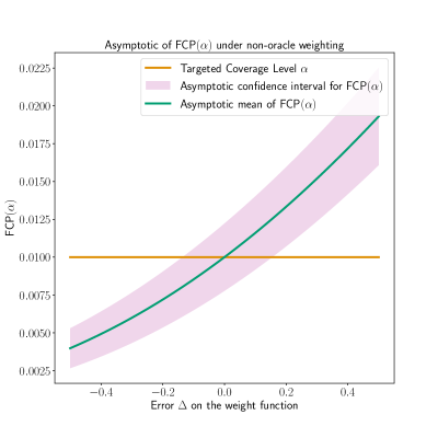
We also obtained a convergence result in case of non-oracle weights (Theorem 3.3), which is crucial to quantify the FCP asymptotic behavior in the difficult but realistic case where the user has not access to the true distribution shift. An illustration in displayed in Figure 2, where the asymptotical confidence interval of the FCP is given in function of an error , measuring how the used weights deviate from the oracle ones. This puts forward that the FCP gets significantly away from when is above or below in this framework.
-
6.
Finally, we obtain similar results for the novelty detection task, by studying the asymptotical behavior of the false discovery proportion (FDP) of classical procedures (Bates et al.,, 2023; Jin and Candès,, 2023), see Section 4. To our knowledge, using a weighted approach has not been considered before in the novelty detection case.
The proofs are based on specific decompositions of the processes that can be found in Section 5, while further details are postponed to appendices.


1.3 Relation to previous work
Conformal prediction is a general pipeline and we refer the reader to Vovk et al., (2005) or Angelopoulos and Bates, (2021) for reviews. We focus here on the inductive/split conformal inference (Papadopoulos et al.,, 2002), where an independent training sample is used to build the predictors, while a calibration sample is used to adjust the prediction sets. All our results can be thought of holding conditionally on the training sample, that is, they hold once the point-predictions have been computed.
The process coincides with the empirical cumulative distribution function (e.c.d.f.) of conformal -values as introduced by Saunders et al., (1999). As recalled above, for a given nominal level , the non-asymptotic distribution of has been obtained in Marques F., (2023); Huang et al., (2024) and the full distribution of the process has been given in Gazin et al., (2024). In addition, Marques F., (2023) gives an asymptotic result for in the regime where tends to infinity only after having made tends to infinity, whereas here we make and grow to infinity independently. In addition, our results are uniform in . Next, in Nguyen et al., (2024), they study a more general risk and also obtained asymptotical results, but only as tends to infinity while is kept fixed.
Finally, we study here novelty detection procedures obtained by applying the Benjamini-Hochberg procedure (, Benjamini and Hochberg,, 1995) to the conformal -values (Mary and Roquain,, 2022; Bates et al.,, 2023; Marandon et al.,, 2024) or to the weighted conformal -values (Tibshirani et al.,, 2019; Barber et al.,, 2023; Jin and Candès,, 2023). Asymptotics for the FDP of such procedures have been extensively studied in the literature, see Genovese and Wasserman, (2002); Neuvial, (2008) for iid uniform -values and Delattre and Roquain, (2011, 2016); Kluger and Owen, (2024) for several types of dependence structures. The present work is in this line of research by seeing (weighted) conformal -values as a particular case of dependent -values, with a very specific dependence structure, induced by the calibration sample. We obtain our results in the novelty detection setting by using the techniques introduced in Neuvial, (2008), that combine functional central limit theorems with the functional delta method. In particular, this provides the full asymptotic FDP distribution for the procedure of Jin and Candès, (2023) (or a variant thereof), for which only in-expectation results were known to our knowledge.
2 Preliminaries
2.1 Prediction setting
We consider the classical split/inductive conformal prediction (Papadopoulos et al.,, 2002). A calibration set is observed with and, given a new point for which only the covariate is observed, a prediction set should be inferred for the outcome 111The regression and classification settings correspond to and finite, respectively.. A non-conformity score function is also given; measures the non-conformity of the response with the covariate . The classical example in regression is the residual where is a regression function trained from an independent training sample (considered as fixed here). The (split) conformal prediction set at level for , denoted by , is defined as
| (3) |
where correspond to the ordered calibration scores . The set can be equivalently described as follows (this classical fact can be retrieved from Lemma F.1): if and only if , where the conformal -value is given by
where .
In this paper, we consider a transductive setting (Vovk,, 2013), where a decision should be made for a whole test sample of size for which only the covariates are observed. We denote the set of the unobserved (since we only observed the covariates of the test points) scores of the test sample. Considering the conformal prediction sets , — corresponding to (3) for all members of the test sample — gives rise to a family of conformal -values defined by
| (4) |
The false coverage proportion of the prediction set family is defined by
| (5) |
Note that this corresponds to the empirical cumulative density function (e.c.d.f.) of the conformal -values family . The following assumption will be considered throughout the paper for the (weighted or not) conformal prediction task.
Assumption 1.
The set of calibration scores and the set of test scores are two independent families of real random variables. The (resp. ) are i.i.d. with distribution (resp. ) and cumulative distribution function (resp. ). Moreover, and are continuous functions.
In the classical setting, the variables , are i.i.d., hence Assumption 1 is true with . Since the vector of scores is exchangeable in this case, the conformal -values are marginally super-uniform (Vovk et al.,, 2005; Romano and Wolf,, 2005) which leads to non-asymptotically valid prediction sets. However, in case of a distribution shift between the distributions of the calibration and the test sample, that is , this property is lost. To solve this issue, Tibshirani et al., (2019); Barber et al., (2023) proposed in this case to use weighted conformal prediction. We follow this approach (with light formal variations for mathematical convenience) by introducing a nonnegative weight function and and the prediction set
where denotes the -quantile of the probability measure , denotes the Dirac measure in and is a normalization constant. The set can also be described with weighted conformal -values thanks to Lemma F.1: if and only if , with
Similarly, with a test sample of size , we obtained the weighted conformal -values,
| (6) |
The of these weighted conformal prediction sets is in this case
| (7) |
which, similarly to (5), is the e.c.d.f. of the weighted conformal -values family.
Finally, under Assumption 1 and if is absolutely continuous with respect to , a particularly interesting weight function, called the oracle weight function, is given by
| (8) |
Clearly, if the calibration and test sample are exchangeable (), the function is constantly equal to . However, under a distribution shift (), the oracle weight function is different, and oracle-weighted conformal -values (6) are different from the regular ones (4). They recover the marginally super-uniform property provided that , see Tibshirani et al., (2019).
2.2 Novelty detection setting
In the novelty detection setting (see for instance Vovk et al.,, 2005; Bates et al.,, 2023), we observe a calibration set of size , with values in distributed according to an unknown “null” distribution and a test sample with either distributed as or not. Formally, we introduce a subset so that when . We also denote . In addition, it is given a non-conformity score function such that measures the non-conformity of the variables with respect to and we denote and the set of the score from the calibration and test samples respectively. A novelty detection procedure decides, for each , whether is a novelty (that is, does not follow ), or not. The procedure described by Bates et al., (2023) consists in computing the conformal -values defined in (4) (by using the specific ’s and ’s of novelty detection), and then applying the Benjamini-Hochberg procedure (Benjamini and Hochberg,, 1995) on this -value family (see Section 5.2.1 for more formal details). This gives a rejection set corresponding to the indices of the declared novelties.
| (9) | ||||
| (10) |
The corresponds to the proportion of errors among the declared novelties (related to a type I error notion), while the corresponds to the proportion of correct decisions among the true novelties (related to a power notion). The following will be assumed throughout the paper for (weighted or not) novelty detection:
Assumption 2.
The set of calibration scores and the set of test scores are two independent families of real random variables. The variables , , are i.i.d. with distribution and c.d.f. . The variables , , are independent, the variables , , are identically distributed as a null score distribution and c.d.f. , and the variables , , are identically distributed as an alternative score distribution (potentially different from ) with c.d.f. . Moreover, , and are continuous.
We also consider the case of a distribution shift between the distribution of the calibration set and the null distribution , in which case we propose to use a weighted -value approach (as for the prediction task). For some weight function and , the weighted conformal -values are the ones from (6) (by using the specific ’s and ’s of novelty detection). We introduce the weighted Bates et al., (2023) procedure as the one applying the BH procedure on this weighted -value family and we denote its rejection set by . We defined as above the and of this procedure.
2.3 Spaces for process convergence
We study the asymptotic convergence of random processes and we consider usual spaces defined in Billingsley, (1999) and van der Vaart and Wellner, (1996), denoted as usual , and , and which are briefly described below.
First, is the set of càdlàg function with the usual Skorohod topology. Second, is the set of càdlàg function with the extended Skorohod topology222This definition is similar to the convergence in considered in Billingsley, (1999) defined as follows: converge to if and only if, for all with such that is continuous at points and , the sequence restricted to converges to restricted to in with the usual Skorohod topology. Finally, is the space of locally bounded function with the topology of the uniform convergence on all compact sets of : a sequence converges to if and only if for all compact subsets of , . We also consider the space of càdlàg function from to with the extended Skorohod topology and the space of locally bounded function from to with the topology of the uniform convergence on all compact sets of .
3 Asymptotics for conformal prediction
The aim here is to study the asymptotic properties of the processes (5) and (7). We study each process in two scenarios: exchangeable or distribution shift.
3.1 Main result
Let us introduce the two following quantities:
| (12) | ||||
| (13) |
where denotes the general inverse of . Formally, and correspond to the c.d.f. of the theoretical -values when and , respectively. We denote denotes the derivative of when it is defined.
Theorem 3.1.
Theorem 3.1 is proved in Section 5.1.4. Note that Theorem 3.1 is true under slightly more general assumptions: namely, it is sufficient that all the scores are exchangeable without ties (Gazin et al.,, 2024). As a corollary, if , this result gives
The latter shows that if the ratio or is small (see Lemma F.2 for the equivalence), the FCP becomes asymptotically over-dispersed. This is markedly different from the case where we have i.i.d. -values uniformly distributed on (compare with the Donsker theorem, see Theorem E.3).
Let us now consider the case where we have potentially a covariate shift, that is, . For this, we consider the following additional assumptions333Assumption 3 can be slightly relaxed, by only assuming that is continuously differentiable on . on and .
Assumption 3.
is increasing on its support with and is continuously differentiable. In addition, is continuously differentiable.
Theorem 3.2.
3.2 Weighted case
Let be a bounded and measurable weight function. To describe the asymptotic behavior of , we need to introduce few additional quantities. First, we let
| (14) |
which corresponds to the c.d.f. of the distribution induced by weight function on the distribution . Note that when choosing the oracle weights (8), the latter is simply the c.d.f. of . Second, let
| (15) |
the c.d.f. of the theoretical -values with , and we denote its derivatives when it exists. Finally, we introduce quantities involved in the variance:
| (16) | ||||
| (17) | ||||
| (18) |
Assumption 4.
The weight function is uniformly bounded by a constant and is measurable. Moreover, is increasing on its support with and is continuously differentiable.
Typically, Assumption 4 holds if is a (possibly infinite) interval of on which is bounded and continuous and satisfies Assumption 3.
Theorem 3.3.
Theorem 3.3 is proved in Section 5.1.5. Note that Theorem 3.3 recovers Theorem 3.2 when . The asymptotic expectation of is which is different from in general, if is chosen arbitrarily. Interestingly, when choosing the oracle weight function given by (8), we have and the convergence in Theorem 3.3 reads as follows:
Theorem 3.4.
This result means that we can recover a result close to Theorem 3.1 in case of a distribution shift if the oracle weight function is used in the prediction sets.
4 Asymptotics for novelty detection
Recall the novelty detection setting of Section 2.2. The aim here is to study the asymptotic properties of the process (9) and of the process (10).
4.1 Additional notation and assumptions
We denote, for all , and the number and the proportion of nulls (i.e. of non-novelties) among tested points, respectively. We introduce the following quantities:
| (19) | ||||
| (20) |
that correspond to the (limiting) c.d.f. of the conformal -values under the null and under the test sample mixture, respectively. For some weight function , we also define their weighted counterparts:
| (21) | ||||
| (22) |
We denote and the derivatives of and , respectively. Note that Assumption 2 with entails . If , we still have when is the oracle weight function.
The two following assumptions are classical when studying the asymptotic of multiple testing procedures (Genovese and Wasserman,, 2002).
Assumption 5.
is strictly concave on .
Assumption 6.
is strictly concave on .
As shown in Chi, (2007); Neuvial, (2008) in the independent case, there is a critical value for the BH procedure given by ; the central limit theorem for the FDP/TDP of BH procedure at level can only be obtained if (for , the BH procedure at level has asymptotically no power). We will show below that this quantity plays a similar role in the (dependent) conformal setting and prove results only if .
4.2 Main results
When (no distribution shift), the following result holds for the regular Bates et al., (2023) procedure.
Theorem 4.1.
Theorem 4.1 is a direct corollary of Proposition 5.3, itself proved in Section 5.2.3. It relies on the pipeline introduced by Neuvial, (2008), which consists in first deriving a functional central limit theorem for the e.c.d.f. of the -values and then to use the functional delta method (van der Vaart,, 1998).
Interestingly, under the assumptions of Theorem 4.1 and if , (25) yields
When (that is ), we note that the FDP convergence is the same as when the -values are independent (Neuvial,, 2008). However, when is bounded, the asymptotic variance is affected by the dependence and gets larger when decreases (that is, decreases). This is coherent with results on FDP convergence in literature dealing with dependency structure: the (positive) dependence is shown to increase the dispersion of the FDP, see Delattre and Roquain, (2011, 2016) among others.
Under distribution shift, the following result holds.
Theorem 4.2.
Theorem 4.2 is proved in Section 5.2.4. The Bates et al., (2023) procedure with (similar) weighted conformal -values has been studied in Jin and Candès, (2023) and they obtained a convergence of FDR and FDP to quantities analogue to and , respectively. By contrast, Theorem 4.2 provides the full asymptotic distribution.
5 Proofs
In this section, we prove the main results of the paper. They rely on a particular decomposition of the FCP/FDP into two processes that further jointly converge. Applying the functional delta method (van der Vaart,, 1998) then allows to conclude.
5.1 Proofs for Section 3
5.1.1 decomposition
To emphasize that the FCP is the e.c.d.f. of , we let for all and ,
| (29) |
We also introduce, for all and ,
| (30) | ||||
| (31) |
corresponding to the e.c.d.f. of the calibration score sample and test score sample, respectively. Note that we have almost surely (under Assumption 1 to ensure that there are no ties almost surely).
5.1.2 Joint convergence
Thanks to (32), in order to obtain a convergence result for , we only need to derive the joint convergence of the two processes delineated in the decomposition (32).
Proposition 5.1.
Proposition 5.1 is proved in Section B.1. The main idea of the proof is to study each coordinate separately and then to use independence to obtain a joint convergence. The process of the first coordinate (test term) is studied by using the Donsker Theorem for and the continuous mapping theorem with a random change of time (Lemma E.10). The second coordinate (calibration term) is investigated by using the Donsker theorem for and then using the functional delta method with the map (Lemma E.5).
5.1.3 Proof of Theorem 3.2
5.1.4 Proof of Theorem 3.1
Up to consider a subsequence, one can assume that . The result thus follows from Theorem 3.2 in the special case , because in this case, and is a standard Brownian bridge.
5.1.5 Proof of Theorem 3.3
For weighted conformal -values, we introduce
| (34) | ||||
| (35) |
the counterparts of (29) and (30) in the weighted case, respectively. Note that almost surely under Assumption 1. Hence, the following decomposition, analogue to (32), holds:
| (36) |
Thus, the novelty of (36) with respect to (32) is only the presence of instead of . By Assumption 4, we can show that the family of function is -Donsker and -Glivenko-Cantelli. Since is Glivenko-Cantelli, the convergence of the test term happens with the same argument in the unweighted case. Because this class is Donsker, using twice the functional delta method gives us that converges in distribution to some known random process on the set . This result is stated and then proved in Lemma C.1. This leads to the joint convergence Proposition C.2, which is the analogue of Proposition 5.1 in the weighted case. Theorem 3.3 is thus proved by applying the continuous mapping theorem to the decomposition (36).
5.2 Proofs for Section 4
5.2.1 expression
We introduced, as in the works from Genovese and Wasserman, (2004) and Neuvial, (2008), and the two e.c.d.f.’s of conformal -values for non-novelties and novelties, respectively:
| (37) | ||||
| (38) |
We also introduce the mixture e.c.d.f. of the test sample
| (39) |
For all , we denote simply (resp. ) the (resp. ) of the procedure rejecting all the conformal -values smaller than , see (9) and (10). The following equalities hold:
Following Neuvial, (2008), and since the novelty detection procedure from Bates et al., (2023) is the procedure applied to conformal -values, we can be described it as a thresholding procedure with threshold , where the functional is defined by
| (40) |
In other words, we have and with the notation above.
5.2.2 Joint convergence and application to the and
Following Neuvial, (2008), and are Hadamard differentiable at provided that is concave and differentiable and that . The following result complete the picture by studying the convergence of .
Proposition 5.2.
Proposition 5.2 is proved in Section B.2. The proof is similar to Proposition 5.1, with the additional technicality that the decomposition (32) should be considered for the two processes and . The fact that these decompositions are based on the same process induces a dependence between the components that results in the term in the asymptotic variance.
By using the functional delta method theorem with the BH functionals described above (see Neuvial, (2008), supplementary files from Delattre and Roquain, (2016) and Lemma S.2.2 from Kluger and Owen, (2024)), we obtain the following result.
Proposition 5.3.
5.2.3 Proof of Theorem 4.1
5.2.4 Proof of Theorem 4.2
6 Conclusion
In this paper we obtained the exact asymptotic distribution of and for conformal inference methods when both the sizes of the calibration sample and test sample grow simultaneously. Our theory covered both the prediction and novelty detection settings, including a potential distribution shift. Our results quantified exactly how the covariance process is affected by the dependence inherent to the conformal settings, that use the same calibration sample for all the test examples. First, we proved that the convergence rate can be largely deteriorated when vanishes to zero (that is, ). Otherwise, when and are of the same order, the convergence rate is the usual one (), but the asymptotic covariance is affected. Nevertheless, when tends to infinity, the convergence is strictly the same as in the usual independent case. Interestingly, our results can be used to calibrate easily and accurately quantiles for controlling an error amount when performing conformal inference with large and . We also quantified the effects of doing conformal inference while there is a distribution shift between the calibration sample and the test sample. We exhibits how this distribution shift acts on the asymptotic behaviour of the , by changing the mean and the variance, and how the correction with weighted conformal -values impacts the asymptotic variance.
While our work paves the way for studying asymptotic convergences in conformal inferences, it left some open directions for future research. For instance, in case of a distribution shift, the oracle weight function is mostly unknown, and is often estimated (Jin and Candès,, 2023). Finding the exact asymptotic distribution for the processes using estimated weights is a very interesting and challenging problem for future investigations.
Acknowledgements
I am grateful to Étienne Roquain for his precious advices and reviews throughout this work. I wish to thank Gilles Blanchard and Sylvain Delattre for their comments, and Magalie Fromont for fruitful discussions. I acknowledge the Emergence project MARS of Sorbonne Université.
References
- Angelopoulos and Bates, (2021) Angelopoulos, A. N. and Bates, S. (2021). A gentle introduction to conformal prediction and distribution-free uncertainty quantification. arXiv preprint arXiv:2107.07511.
- Balasubramanian et al., (2014) Balasubramanian, V., Ho, S.-S., and Vovk, V. (2014). Conformal prediction for reliable machine learning: theory, adaptations and applications. Morgan Kaufmann books.
- Barber et al., (2023) Barber, R. F., Candes, E. J., Ramdas, A., and Tibshirani, R. J. (2023). Conformal prediction beyond exchangeability. The Annals of Statistics, 51(2):816–845.
- Bates et al., (2023) Bates, S., Candès, E., Lei, L., Romano, Y., and Sesia, M. (2023). Testing for outliers with conformal p-values. Ann. Statist., 51(1):149–178.
- Benjamini and Hochberg, (1995) Benjamini, Y. and Hochberg, Y. (1995). Controlling the false discovery rate: a practical and powerful approach to multiple testing. J. Roy. Statist. Soc. Ser. B, 57(1):289–300.
- Billingsley, (1999) Billingsley, P. (1999). Convergence of probability measures. Wiley Series in Probability and Statistics: Probability and Statistics. John Wiley & Sons Inc., New York, second edition. A Wiley-Interscience Publication.
- Chi, (2007) Chi, Z. (2007). On the performance of FDR control: constraints and a partial solution. Ann. Statist., 35(4):1409–1431.
- Delattre and Roquain, (2011) Delattre, S. and Roquain, E. (2011). On the false discovery proportion convergence under Gaussian equi-correlation. Statist. Probab. Lett., 81(1):111–115.
- Delattre and Roquain, (2016) Delattre, S. and Roquain, E. (2016). On empirical distribution function of high-dimensional Gaussian vector components with an application to multiple testing. Bernoulli, 22(1):302–324.
- Donsker, (1952) Donsker, M. D. (1952). Justification and extension of Doob’s heuristic approach to the Komogorov-Smirnov theorems. Ann. Math. Statistics, 23:277–281.
- Gazin et al., (2024) Gazin, U., Blanchard, G., and Roquain, E. (2024). Transductive conformal inference with adaptive scores. In Dasgupta, S., Mandt, S., and Li, Y., editors, Proceedings of The 27th International Conference on Artificial Intelligence and Statistics, volume 238 of Proceedings of Machine Learning Research, pages 1504–1512. PMLR.
- Genovese and Wasserman, (2002) Genovese, C. and Wasserman, L. (2002). Operating characteristics and extensions of the false discovery rate procedure. J. R. Stat. Soc. Ser. B Stat. Methodol., 64(3):499–517.
- Genovese and Wasserman, (2004) Genovese, C. and Wasserman, L. (2004). A stochastic process approach to false discovery control. Ann. Statist., 32(3):1035–1061.
- Huang et al., (2024) Huang, K., Jin, Y., Candes, E., and Leskovec, J. (2024). Uncertainty quantification over graph with conformalized graph neural networks. Advances in Neural Information Processing Systems, 36.
- Jin and Candès, (2023) Jin, Y. and Candès, E. J. (2023). Model-free selective inference under covariate shift via weighted conformal p-values. arXiv preprint arXiv:2307.09291.
- Kluger and Owen, (2024) Kluger, D. M. and Owen, A. B. (2024). A central limit theorem for the benjamini-hochberg false discovery proportion under a factor model. Bernoulli, 30(1):743–769.
- Marandon et al., (2024) Marandon, A., Lei, L., Mary, D., and Roquain, E. (2024). Adaptive novelty detection with false discovery rate guarantee. The Annals of Statistics, 52(1):157 – 183.
- Marques F., (2023) Marques F., P. C. (2023). On the universal distribution of the coverage in split conformal prediction. arXiv preprint 2303.02770.
- Mary and Roquain, (2022) Mary, D. and Roquain, E. (2022). Semi-supervised multiple testing. Electronic Journal of Statistics, 16(2):4926 – 4981.
- Neuvial, (2008) Neuvial, P. (2008). Asymptotic properties of false discovery rate controlling procedures under independence. Electron. J. Stat., 2:1065–1110.
- Nguyen et al., (2024) Nguyen, D. T., Pathak, R., Angelopoulos, A. N., Bates, S., and Jordan, M. I. (2024). Data-adaptive tradeoffs among multiple risks in distribution-free prediction. arXiv preprint arXiv:2403.19605.
- Papadopoulos et al., (2002) Papadopoulos, H., Proedrou, K., Vovk, V., and Gammerman, A. (2002). Inductive confidence machines for regression. In 13th European Conference on Machine Learning (ECML 2002), pages 345–356. Springer.
- Romano and Wolf, (2005) Romano, J. P. and Wolf, M. (2005). Exact and approximate stepdown methods for multiple hypothesis testing. J. Amer. Statist. Assoc., 100(469):94–108.
- Saunders et al., (1999) Saunders, C., Gammerman, A., and Vovk, V. (1999). Transduction with confidence and credibility. In 16th International Joint Conference on Artificial Intelligence (IJCAI 1999), pages 722–726.
- Shorack and Wellner, (1986) Shorack, G. R. and Wellner, J. A. (1986). Empirical processes with applications to statistics. Wiley Series in Probability and Mathematical Statistics: Probability and Mathematical Statistics. John Wiley & Sons Inc., New York.
- Storey, (2002) Storey, J. D. (2002). A direct approach to false discovery rates. J. R. Stat. Soc. Ser. B Stat. Methodol., 64(3):479–498.
- Tibshirani et al., (2019) Tibshirani, R. J., Foygel Barber, R., Candes, E., and Ramdas, A. (2019). Conformal prediction under covariate shift. Advances in neural information processing systems, 32.
- van der Vaart, (1998) van der Vaart, A. W. (1998). Asymptotic statistics, volume 3 of Cambridge Series in Statistical and Probabilistic Mathematics. Cambridge University Press, Cambridge.
- van der Vaart and Wellner, (1996) van der Vaart, A. W. and Wellner, J. A. (1996). Weak convergence and empirical processes. Springer Series in Statistics. Springer-Verlag, New York. With applications to statistics.
- Vovk, (2013) Vovk, V. (2013). Transductive conformal predictors. In Artificial Intelligence Applications and Innovations: 9th IFIP WG 12.5 International Conference (AIAI 2013), pages 348–360. Springer.
- Vovk et al., (2005) Vovk, V., Gammerman, A., and Shafer, G. (2005). Algorithmic learning in a random world. Springer.
Appendix A Standardisation lemma
In this section, we introduce the standardisation lemma, which will be extensively used in our proofs. Let us introduce the notation
| (41) | ||||
| (42) |
where by convention denotes the infimum of the support of the distribution given by and . The following lemma holds.
Lemma A.1.
Consider either the prediction setting with Assumption 1 (with parameters , ) or the novelty detection setting with Assumption 2 (with parameters , , ). If , satisfy Assumption 3, for any weight function with , the distribution of the -weighted conformal -value family under the parameters , (and ) is the same as the -weighted conformal -value family under the parameters , (and ).
Proof of Lemma A.1.
Since is continuous increasing on its support, we can write almost surely
with which are iid uniform and which are iid (or either under the null or under the alternative, in the novelty detection setting). ∎
Appendix B Proofs of auxiliary results
In this section, we prove Proposition 5.1, Propositions 5.2 and 5.3. Proofs for the weighted case are given in Section C.
B.1 Proof of Proposition 5.1
First, the Donsker theorem (Theorem E.3) provides
with being a standard Brownian bridge. Moreover, by the Glivenko-Cantelli theorem, we have that converges in probability on to . Since by Assumption 3 the inverse map is continuous at we obtain that converges in probability on to .
Second, applying again the Donsker theorem (Theorem E.3), we have
with a standard Brownian bridge independent of . Now, by using the fonctional delta method with the inverse map (see Lemma E.6) by Assumption 3, we obtain,
| (43) |
where denotes the derivative of . Again, we use the Hadamard differentiability of the map which is true by Assumption 3 (see Lemma E.5) to obtain
Since for all , and since is a standard Brownian bridge if and only if is a standard Brownian bridge we obtain the second term in (33) .
B.2 Proof of Proposition 5.2
By using Lemma A.1, one can assume without loss of generality that and has for c.d.f. . By applying the Donsker theorem (Theorem E.3) with the independent families , and and following the same reasoning as in the proof of Proposition 5.1, there exist , and three independent standard Brownian bridges such that
where we denoted the e.c.d.f. of for . Now, by using Lemma E.10 (or more precisely, an obvious extension of it for joint processes), we obtain
B.3 Proof of Proposition 5.3
By Assumption 5, and since , the asymptotic threshold is well defined and belongs to . Now observe that there exists a compact interval such that
| (44) |
To see this, note that since we have that , hence is smaller than any . Now, since , any leads to , which leads to (44).
Now consider the functional
| (45) |
which is similar to (40) but with a restricted range on . Equation (44) hence reads as . In addition, we have
| (46) |
where , which is positive by the choice of . Indeed, if , we have , which implies that . This proves (46).
Now, is Hadamard differentiable at , tangentially to with a derivative coinciding with the one of , that is,
By the convergence of Proposition 5.2, which holds on , we can apply the functional delta method (see Lemma E.9 for the exact expression of derivatives) to obtain
where , and are the three processes defined in Proposition 5.2. Now, the same convergences hold for by using (46) because converges in probability to . This concludes the proof.
Appendix C Proofs for the weighted case
C.1 Weighted versions of the Glivenko-Cantelli and Donsker theorem.
Recall that is given by (35). The next result applies both in the prediction and novelty detection settings and will be used to prove Propositions C.2, C.3 and C.4..
Lemma C.1.
Assume . Let a weight function satisfying Assumption 4. Then it holds
and
where is a standard Brownian bridge and an independent standard Gaussian random variable.
Note that in the case (unweighted case), we recover the convergence presented in Corollary E.7, because .
Proof of Lemma C.1.
Denote for and ,
Since is uniformly bounded, the family is -Glivenko-Cantelli, and converges uniformly on in probability to the function given by (Shorack and Wellner,, 1986). Then, by continuity at of the map of Lemma E.8, we get that converges uniformly (in probability) to . Since tends uniformly to a.s., converges uniformly (in probability) to . By continuity of the inverse map at (see Lemma E.6), we obtain that converges in probability to on . This proves the first statement.
Next, we turn to prove the second statement. Since is uniformly bounded, the family is -Donsker (Shorack and Wellner,, 1986). hence there exist a Gaussian process such that
where the distribution of is given by and for ,
where we used and by the definition of (17), (16) and (14). We easily check that the condition of the Kolmogorov-Čentsov theorem is satisfied, so that has a continuous version. Now, by applying the functional delta method with the map of Lemma E.8, we obtain
Since a.s., then by Slustky’s lemma, we obtain
And by applying the functional delta method with the inverse map at (see Lemma E.6) we obtain,
To conclude, we identify the covariance of the Gaussian limiting process. For, ,
Therefore, the last display is equal to
The first term coincides with the covariance term of for a standard Brownian bridge , while the second term is the covariance of the process with . This concludes the proof for the second statement.
∎
C.2 Prediction setting
The following result is the weighted version of Proposition 5.1.
Proposition C.2.
Proof.
By the Donsker theorem (Theorem E.3), we have
where is a standard Brownian bridge. By Lemma C.1 (which applies because we can standardize the calibration set, see Lemma A.1), we have
where is a standard Brownian bridge and is an independent standard Gaussian random variable. Thus, by independence between and ,
where and two independent Brownian bridges and an independent Gaussian r.v.. By Lemma C.1, we have that on hence by using Lemma E.10 we get
which concludes the proof.
∎
C.3 Novelty detection setting
We define
the counterparts of (37) and (38), respectively. Hence, the mixture e.c.d.f.
is the counterpart of (39).
The following result is the weighted version of Proposition 5.2 (with an oracle weight function).
Proposition C.3.
In the novelty detection setting with Assumption 2, assume that is absolutely continuous with respect to and that the oracle weight function (11) satisfies Assumption 4. Under Assumption 3, assuming that and , we have
with and three independent Brownian bridges and an independent standard Gaussian random variable . Furthermore,
Proof.
We apply twice the argument of the proof of Proposition C.2 to the null and the alternative processes to obtain , and three independent standard Brownian bridge and an independent standard Gaussian r.v. such that,
converges when in distribution to
We conclude by using the decomposition (36) on and , the Slutsky lemma and the continuous mapping theorem. ∎
The following result is the weighted version of Proposition 5.3.
Proposition C.4.
Under Assumption 2, assume that is absolutely continuous with respect to and that the oracle weight function (11) satisfies Assumption 4. Under Assumptions 3, and 6, assuming that the targeted level , assuming that and , we have,
where , and are the three processes defined in Proposition C.3.
Appendix D Weighted novelty detection for a general weight function
In this section, we extend Propositions C.3 and C.4 to the case of a general weight function. We should add the following technical assumption (which was implicitly satisfied in the oracle case):
Assumption 7.
is continuously differentiable.
Let us introduce
where corresponds to the positive false discovery rate at (Storey,, 2002). Note that in the oracle case , but is not necessarily zero for a general .
Proposition D.1.
The proof of Proposition D.1 is omitted because it is completely analogue to the one of Proposition C.3.
Theorem D.2.
Appendix E Additional tools for asymptotics
E.1 Donsker and Glivenko-Cantelli theorems
Theorem E.1 (Glivenko-Cantelli).
Let be a c.d.f., and be an empirical version of with i.i.d. points. Then,
Proposition E.2.
Let be i.i.d. random variables uniformly distributed over . Denote the e.c.d.f. the family . Then,
Theorem E.3 (Donsker, (1952)).
Let iid real random variables. Let the cumulative distribution function of and the empirical cdf of . Then,
with a standard Brownian bridge.
Proposition E.4.
Let a weight function satisfying Assumption 4. Then the family of function is -Donsker and -Glivenko-Cantelli.
E.2 Hadamard differentiability
The three first results below can be found in van der Vaart, (1998).
Lemma E.5.
Let be a continuously differentiable function. The map with entries being functions contained in is Hadamard differentiable tangentially to with derivative:
Assumption 8.
The cumulative distribution function have a compact support in the sense that that for all , , for all , and for all , . Furthermore, is continuously differentiable on with stricly positive derivative.
Lemma E.6.
Let satisfying Assumption 8. Then the inverse map with domain the set of cumulative distribution function of probability measure on with value in is Hadamard differentiable at tangentially to with derivative being the map
Corollary E.7.
Let be iid real random variables. Let be the cumulative distribution function of and be the empirical cdf of . Denote and the corresponding quantile functions. Assume that satisfies Assumption 8 with derivative . Then,
with being a standard Brownian bridge.
Lemma E.8.
Let a weight function satisfying Assumption 4. Denote . The map is Hadamard differentiable at tangentially to with the following formula:
with .
Proof of Lemma E.8.
Let defined as in the statement. Let be a family of function in with uniformly on . We have, for small enough,
Hence, we obtain
which prove the Hadamard differentiability. ∎
We gather below the formulas of the Hadamard derivatives of the functionals of interest when studying the asymptotic of the . They are obtained from Neuvial, (2008).
Lemma E.9.
Let be a continuously differentiable increasing strictly concave function. If , then is Hadamard differentiable at tangentially to with the following expression for all
Let be two continuously differentiable c.d.f. functions from to and let such that is stricly concave. Let . In addition, let us define
| (47) | ||||
| (48) |
where . Then, , and are Hadamard differentiable at tangentially to with the following derivative expressions: for all ,
where .
E.3 Random change of time
We present here a version of the random change of time lemma of Billingsley, (1999) (page 151), which is adapted to the topological spaces , and .
Lemma E.10.
Let be a sequence of random processes in , and two random processes in and , respectively, which are both a.s. continuous and such that in . Let be a sequence of random processes in and such that converges in probability to on . Assume that for all , . Then,
Proof of Lemma E.10.
Since and are continuous, converges in distribution to on by Lemma E.12. Hence, by Slutsky’s lemma, the sequence converges in distribution to on . Hence by Lemma E.11 and the continuous mapping theorem we obtain,
Since is continuous, then is in and the previous convergence implies the convergence in . ∎
Note that when using Lemma E.10 in our work, the convergence of the sequence is typically given by the Donsker Theorem, while the convergence of is given by the Glivenko-Cantelli theorem.
Lemma E.11.
Define the following map . For all and , is continuous at .
Proof of Lemma E.11.
Let and . Let a sequence in which converges to . Let be a compact set. Let . The set is bounded since and and belongs in , hence is included in a compact set of . Since is continuous, we have such that for all , implies that . Let such that for all , and . Then for all ,
where the first appears since for all , , and . Furthermore for all a compact subset of , . Hence, is continuous at . ∎
Finally, the following result is classical and shows how a convergence in distribution on can imply a uniform convergence (Billingsley,, 1999), with the local topology defined in Section 2.3.
Lemma E.12 (Billingsley, (1999)).
Let be a sequence of random processes on . Let be a continuous function a.s.. Then, converges in distribution to on if and only if converges in distribution to on
Appendix F Useful Lemmas
Lemma F.1.
Let , be a family of positive weight summing to and be a probability measure on . Define for all , the -quantile of the probability measure . Then, for all and , the two following assertions are equivalent:
-
(i)
-
(ii)
Proof of Lemma F.1.
First note that, since the weights are summing to , (i) is equivalent to . Now prove that (ii) implies (i). If , then and thus (i) holds.
Conversely, if (i) holds, we have and thus
exists. With such a we have . This proves by definition of the quantile function. Hence and we have proved (ii).
∎
Lemma F.2.
if and only if .