A lightweight, geometrically flexible fast algorithm for the evaluation of layer and volume potentials

Abstract

Over the last two decades, several fast, robust, and high-order accurate methods have been developed for solving the Poisson equation in complicated geometry using potential theory. In this approach, rather than discretizing the partial differential equation itself, one first evaluates a volume integral to account for the source distribution within the domain, followed by solving a boundary integral equation to impose the specified boundary conditions.

Here, we present a new fast algorithm which is easy to implement and compatible with virtually any discretization technique, including unstructured domain triangulations, such as those used in standard finite element or finite volume methods. Our approach combines earlier work on potential theory for the heat equation, asymptotic analysis, the nonuniform fast Fourier transform (NUFFT), and the dual-space multilevel kernel-splitting (DMK) framework. It is insensitive to flaws in the triangulation, permitting not just nonconforming elements, but arbitrary aspect ratio triangles, gaps and various other degeneracies. On a single CPU core, the scheme computes the solution at a rate comparable to that of the fast Fourier transform (FFT) in work per gridpoint.

1 Introduction

In this paper, we consider the solution of the Poisson equation

(1) $$-\Delta u(\bm{x}) =f(\bm{x})\quad\text{for }\bm{x}\in\Omega,$$

where $\Omega\subset\mathbb{R}^{2}$ is either an interior or exterior domain, subject to either Dirichlet or Neumann boundary conditions:

(2) $$u(\bm{x})=g(\bm{x})\quad\text{for }\bm{x}\in\partial\Omega,$$

or

(3) $$\frac{\partial u}{\partial\nu}(\bm{x})=g(\bm{x})\quad\,\text{for }\bm{x}\in\partial\Omega,$$

respectively. Here, $u$ is an unknown function, $\frac{\partial u}{\partial\nu}$ denotes its outward normal derivative, $f$ is a smooth source density in $\Omega$, and $g$ is the specified boundary data. We will focus on integral equation methods, and will seek a representation of the solution as a combination of volume and layer potentials. The volume potential $\mathcal{V}[f](\bm{x})$ is defined by

(4) $$\mathcal{V}[f](\bm{x})\equiv\int_{\Omega}\!G(\bm{x}-\bm{x^{\prime}})f(\bm{x^{\prime}})\,\mathrm{d}\bm{x^{\prime}}\quad\text{for }\bm{x}\in\Omega,$$

where

(5) $$G(\bm{x})=-\frac{1}{2\pi}\log\|\bm{x}\|,$$

is the fundamental solution for the Poisson equation in two dimension, with $\|\bm{x}\|$ denoting the Euclidean norm of $\bm{x}\in\mathbb{R}^{2}$. Single and double layer potentials are defined by

(6) $$\mathcal{S}[\sigma](\bm{x})\equiv\int_{\partial\Omega}\!G(\bm{x}-\bm{x^{\prime}})\sigma(\bm{x^{\prime}})\,\mathrm{ds}_{\bm{x^{\prime}}}\quad\text{for }\bm{x}\in\Omega,$$

and

(7) $$\mathcal{D}[\mu](\bm{x})\equiv\int_{\partial\Omega}\!\frac{\partial G}{\partial{\nu}_{\bm{x^{\prime}}}}(\bm{x}-\bm{x^{\prime}})\mu(\bm{x^{\prime}})\,\mathrm{ds}_{\bm{x^{\prime}}}\quad\text{for }\bm{x}\in\Omega,$$

respectively. Here, $\bm{\nu}(\bm{x^{\prime}})=(\nu_{1}(\bm{x^{\prime}}),\nu_{2}(\bm{x^{\prime}}))$ is the outward unit normal at a point $\bm{x^{\prime}}\in\partial\Omega$, and $\frac{\partial G}{\partial{\nu}_{\bm{x^{\prime}}}}(\bm{x}-\bm{x^{\prime}})$ denotes the normal derivative of the fundamental solution at $\bm{x^{\prime}}$. The functions $\sigma(\bm{x^{\prime}})$ and $\mu(\bm{x^{\prime}})$ are supported on the boundary $\partial\Omega$, and will be referred to as single and double layer densities. Note that $\mathcal{S}[\sigma](\bm{x})$ and $\mathcal{D}[\mu](\bm{x})$ define harmonic functions in $\Omega$ while $\mathcal{V}[f](\bm{x})$ satisfies the Poisson equation. Letting $\bm{x}=\bm{x^{\prime}}\pm r\bm{\nu}(\bm{x^{\prime}})$, it is well-known that the double layer potential satisfies the jump relations

(8) $$\lim_{r\rightarrow 0^{+}}\mathcal{D}[\mu](\bm{x^{\prime}}\pm r\bm{\nu}(\bm{x^{\prime}}))=\mathcal{D}[\mu](\bm{x^{\prime}})\pm\frac{1}{2}\mu(\bm{x^{\prime}}).$$

For the interior Dirichlet problem in a simply connected region, standard potential theory [38, 43, 55, 69] suggests a representation for the solution $u$ of the form

(9) $$u(\bm{x})=\mathcal{V}[f](\bm{x})+\mathcal{D}[\mu](\bm{x})\quad\text{for }\bm{x}\in\Omega,$$

where $\mu$ is unknown and to be determined by the boundary condition. For the Neumann problem, we will use Green’s representation formula:

(10) $$u(\bm{x})=\mathcal{V}[f](\bm{x})+\mathcal{S}\left[\frac{\partial u}{\partial{\nu}}\right](\bm{x})-\mathcal{D}[u](\bm{x})\quad\text{for }\bm{x}\in\Omega.$$

Taking the limits of the representations (9) and (10) as $\bm{x}$ approaches a point on the boundary leads to boundary integral equations, which will be described in Section 5.

An important feature of the potential theory approach is that $\mathcal{V}[f](\bm{x})$ is an integral transform over the volumetric data; that is, no unknowns are introduced in the domain interior. The difference $v(\bm{x})=u(\bm{x})-\mathcal{V}[f](\bm{x})$ is harmonic (satisfying the Laplace equation). Thus, one can think of the layer potential contributions in (9) and (10) as representing a harmonic correction to $\mathcal{V}[f](\bm{x})$, needed to enforce (2) or (3). Any “particular solution” that satisfies the inhomogeneous equation (1) can be used in place of $\mathcal{V}[f](\bm{x})$.

We do not seek to review the literature here, but briefly summarize the various integral equation methods that are currently available to put our new solver in context. First, if the right-hand side $f(\bm{x})$ is not too complicated, one can attempt to find a particular solution $F(\bm{x})$ such that

(11) $$-\Delta F(\bm{x})=f(\bm{x}).$$

The function $F(\bm{x})$ in (11) is called an anti-Laplacian of $f$ and one can represent $u(\bm{x})$ in the form $u(\bm{x})=v(\bm{x})+\mathcal{V}[f](\bm{x})$ where $v(\bm{x})$ and represented via layer potentials (see Section 5). Using a global anti-Laplacian in this manner is sometimes called the dual reciprocity method [58]. Unfortunately, it is only practical when $f(\bm{x})$ has a simple analytical representation. To address problems where the volumetric data $f(\bm{x})$ is represented on a more complex data structure, fast algorithms are required, as the naive cost of computing a volume integral with $N$ discretization points at the same $N$ locations is of the order $O(N^{2})$. For uniform grids in complicated geometry, careful attention to finite difference approximations at points near the domain boundary was shown to permit fast solvers based on the fast Fourier transform (FFT) to compute volume potentials with the order of accuracy of the underlying finite difference approximation [53, 54]. These are related to immersed boundary and immersed interface methods [49, 59]. Subsequently, adaptive fast algorithms for the direct computation of volume integrals began to emerge in the 1990s (see, for example, [17, 27, 36, 48, 51]). These methods generally assume the right-hand side is provided on an adaptive quadtree or octtree data structure (for 2D and 3D problems, respectively) without a complicated boundary.

Remark 1.1.

We will refer to fast algorithms for computing volume potentials on adaptive quad or octtrees (but without a complicated boundary) as box codes.

When the source distribution in an irregular region is nonuniform, at least three distinct approaches are under active investigation. These include: (1) function extension methods that enable the straightforward application of box codes [6, 19, 33, 32, 25, 31, 71, 72], (2) composite or overlapping grid methods which use a box code for leaf nodes away from the boundary, but a different data structure near the boundary [4, 70], and (3) domain triangulation methods, which modify the fast multipole method (FMM) but do not make use of box codes at all. The latter approach has the advantage of making the solver compatible with the discretizations used in finite element and finite volume methods, but has received less attention from the integral equation community. An early exception is [62] which coupled the FMM with adaptive quadrature to compute $\mathcal{V}[f](\bm{x})$. Recently, Shen and Serkh [65] developed a high-order accurate FMM that computes an anti-Laplacian on each triangle and enforces global continuity by means of layer potentials on triangle boundaries. This extends the box code approach of [36] to general geometries with good performance. See also the recent interpolatory method of [3].

Since there are now many linear scaling schemes for computing volume integrals, the reader might well ask why we seek to develop a new approach. The answer is that there is still a need for a fast solver that is easy to implement, robust, highly efficient, and compatible with virtually any discretization. In this paper, we attempt to meet these criteria, achieving speeds near that of the FFT in work per gridpoint. Our method, illustrated using unstructured triangulations, does not make use of FMM acceleration. Instead, we blend the nonuniform FFT (NUFFT) with “kernel splitting” and asymptotics, extending the dual-space multilevel kernel-splitting (DMK) framework of [42] to complicated geometries. Moreover, we show that both volume and layer potentials can be evaluated accurately with the new scheme in a manner that is insensitive to flaws in the triangulation, permitting nonconforming and arbitrary aspect ratio elements, gaps and various other degeneracies (see Fig. 7).

An essential ingredient in our method is the use of asymptotic expansions, described in Section 4. For layer potentials, this extends the ideas presented in [37, 50, 73, 77]. Similar asymptotic analysis has also been carried out by Beale et al. (see, for example, [13, 14, 15]), although used in a somewhat different manner. As far as we are aware, the use of asymptotic expansions for volume integrals, as described below, has not been considered before. (See also Remark 4.9.)

2 Mathematical preliminaries

Our fast algorithm for the evaluation of volume and layer potentials is naturally motivated by first observing that the volume integral $\mathcal{V}[f](\bm{x})$ in Eq. 4 can be computed as the steady state limit of the heat equation [30, 60]

(12) $$u_{t}(\bm{x})-\Delta u(\bm{x})=f(\bm{x}).$$

We may view this limit as the solution at time $t=0$ for the equation (12) with zero initial data at time $t=-\infty$. Using the fundamental solution for the heat equation in two dimensions

$$K(\bm{x},t)=\frac{e^{-\|\bm{x}\|^{2}/4t}}{4\pi t},$$

we write this alternative representation as a volume heat potential (where large time corresponds to a large time in the past):

(13) $$\mathcal{V}[f](\bm{x})=\int_{0}^{\infty}\!\int_{\Omega}\!\frac{e^{-\|\bm{x-x^{\prime}}\|^{2}/4t}}{4\pi t}\,f(\bm{x^{\prime}})\,\mathrm{d}\bm{x^{\prime}}\,\mathrm{d}t.$$

This is the function we will compute but divided into three contributions. We let

(14) $$\mathcal{V}[f](\bm{x})=\mathcal{V}_{L}[f](\bm{x})+\mathcal{V}_{NH}[f](\bm{x})+\mathcal{V}_{FH}[f](\bm{x})\,,$$

where

(15) $$\mathcal{V}_{L}[f](\bm{x}) =\int_{0}^{\delta_{1}}\!\int_{\Omega}\!\frac{e^{-\|\bm{x-x^{\prime}}\|^{2}/4t}}{4\pi t}\,f(\bm{x^{\prime}})\,\mathrm{d}\bm{x^{\prime}}\,\mathrm{d}t,\quad\mathcal{V}_{NH}[f](\bm{x})\!\!\!\! =\int^{\delta_{2}}_{\delta_{1}}\!\int_{\Omega}\!\frac{e^{-\|\bm{x-x^{\prime}}\|^{2}/4t}}{4\pi t}\,f(\bm{x^{\prime}})\,\mathrm{d}\bm{x^{\prime}}\,\mathrm{d}t,$$

$$\mathcal{V}_{FH}[f](\bm{x}) =\int^{\infty}_{\delta_{2}}\!\int_{\Omega}\!\frac{e^{-\|\bm{x-x^{\prime}}\|^{2}/4t}}{4\pi t}\,f(\bm{x^{\prime}})\,\mathrm{d}\bm{x^{\prime}}\,\mathrm{d}t.$$

$\mathcal{V}_{L}$ accounts for contributions that are local in time, $\mathcal{V}_{NH}$ accounts for contributions from the near history, and $\mathcal{V}_{FH}$ accounts for contributions from the far history. Such a decomposition was proposed in [37] for the rapid evaluation of layer heat potentials, and used in the manner suggested above in [73] for harmonic potentials of the form (6) and (7). In those papers, the near and far history were treated together as the “history” part:

(16) $$\mathcal{V}_{H}[f](\bm{x})=\mathcal{V}_{NH}[f](\bm{x})+\mathcal{V}_{FH}[f](\bm{x})\,.$$

Remark 2.1.

The DMK framework of [42] was introduced as an alternative to box codes (among other things). It is a hierarchical, adaptive, Fourier-based method that, in the present context, can be viewed as using $O(\log N)$ levels of subdivision with respect to the time variable together with an adaptive quadtree data structure. Our work here combines kernel splitting with asymptotics to evaluate the convolution of the harmonic Green’s function with nonsmooth distributions (i.e., layer and volume potentials in complicated geometry). For the sake of simplicity, we restrict ourselves to quasi-uniform discretizations and a two-level implementation, accelerated by the NUFFT instead of the full DMK machinery. We will return to this topic in Section 7.

It should be noted that the decomposition of a volume heat potential in two pieces, namely $\mathcal{V}[f](\bm{x})=\mathcal{V}_{L}[f](\bm{x})+\mathcal{V}_{H}[f](\bm{x})$ is essentially the basis for Ewald summation [28], although originally developed for discrete sources in three dimensions with periodic boundary conditions, rather than continuous distributions in free space. In Ewald’s treatment, modified for the two dimensional setting, the basic idea is that of kernel splitting: expressing the Green’s function as

(17) $$G(\bm{x})=-\frac{1}{2\pi}\log\|\bm{x}\|=G_{H}[\delta](\bm{x})+G_{L}[\delta](\bm{x})\,,$$

with

(18) $$G_{H}[\delta](\bm{x})=\left[-\frac{1}{2\pi}\log\|\bm{x}\|-\frac{1}{4\pi}E_{1}\!\left(\frac{\|\bm{x}\|^{2}}{4\delta}\right)\right]\quad,\quad G_{L}[\delta](\bm{x})=\frac{1}{4\pi}E_{1}\!\left(\frac{\|\bm{x}\|^{2}}{4\delta}\right)\,,$$

where

$$E_{1}(x)=\int_{1}^{\infty}\frac{e^{-tx}}{t}\,\mathrm{d}t$$

is the exponential integral function [56]. The connection between the decomposition in terms of heat potentials and kernel splitting is established by the identity

(19) $$\int_{0}^{\delta}\!\frac{e^{-\|\bm{x}\|^{2}/4t}}{4\pi t}\,\mathrm{d}t=\frac{1}{4\pi}E_{1}\!\left(\frac{\|\bm{x}\|^{2}}{4\delta}\right)$$

for $\bm{x}\neq 0$. We refer the reader to [1, 37, 42, 50, 57, 64, 73] for further discussion.

It remains only to understand how each of the terms in (14) is to be computed. Simply stated, $\mathcal{V}_{L}[f](\bm{x})$ is local in both space and time and will be treated using asymptotics, while $\mathcal{V}_{NH}[f](\bm{x})$ and $\mathcal{V}_{FH}[f](\bm{x})$ will be computed using Fourier methods.

Definition 2.2.

For a function $f(\bm{x})$ in two dimensions, we define its Fourier transform by

$$\hat{f}(\bm{k})=\int_{\bm{x}\in\mathbb{R}^{2}}e^{-i\bm{k}\cdot\bm{x}}f(\bm{x})\,\mathrm{d}\bm{x},$$

where $\bm{k}\in\mathbb{R}^{2}$. The function $f(\bm{x})$ is recovered from $\hat{f}(\bm{k})$ by the inverse transform

$$f(\bm{x})=\frac{1}{(2\pi)^{2}}\int_{\bm{k}\in\mathbb{R}^{2}}e^{i\bm{k}\cdot\bm{x}}\hat{f}(\bm{k})\,\mathrm{d}\bm{k}.$$

Lemma 2.3.

For a function $f(\bm{x})$ compactly supported in $\Omega$, the near history component has the Fourier representation

(20) $$\mathcal{V}_{NH}[f](\bm{x})=\int_{\bm{k}\in\mathbb{R}^{2}}\frac{e^{-\|\bm{k}\|^{2}\delta_{1}}-e^{-\|\bm{k}\|^{2}\delta_{2}}}{\|\bm{k}\|^{2}}e^{i\bm{k\cdot x}}\hat{f}(\bm{k})\,\mathrm{d}\bm{k}.$$

Proof 2.4.

This result follows from the fact that the Fourier transform of ${e^{-\|\bm{x}\|^{2}/4t}}/(4\pi t)$ is $e^{-\|\bm{k}\|^{2}t}$, the convolution theorem, and integration in time.

Note that the integrand in (20) is rapidly decaying in Fourier space and that it is infinitely differentiable, since the expression

$$\frac{e^{-\|\bm{k}\|^{2}\delta_{1}}-e^{-\|\bm{k}\|^{2}\delta_{2}}}{\|\bm{k}\|^{2}}$$

has a convergent power series and $f(\bm{x})$ is assumed to have compact support.

The far history is a little more delicate, as its Fourier transform has a singularity of the order $1/\|\bm{k}\|^{2}$ at the origin and its rigorous analysis would involve consideration of tempered distributions. Using the method of [75], however, we have the following lemma.

Lemma 2.5.

Suppose that $f(\bm{x})$ is compactly supported in $\Omega\subset[-1,1]^{2}$. Then, for $\bm{x}$ with $\|\bm{x}\|\leq 1$, $\mathcal{V}_{FH}[f](\bm{x})$ has the Fourier representation

(21) $$\mathcal{V}_{FH}[f](\bm{x})\approx\int_{\bm{k}\in\mathbb{R}^{2}}e^{-\|\bm{k}\|^{2}\delta_{2}}W(\bm{k})e^{i\bm{k\cdot x}}\hat{f}(\bm{k})\,\mathrm{d}\bm{k},$$

where

(22) $$W(\bm{k})=\left[\frac{1-J_{0}(2\sqrt{2}\,\|\bm{k}\|)}{\|\bm{k}\|^{2}}-\frac{2\sqrt{2}\log(2\sqrt{2})\,J_{1}(2\sqrt{2}\,\|\bm{k}\|)}{\|\bm{k}\|}\right],$$

with $J_{0}$ and $J_{1}$ denoting Bessel functions of the first kind. The error in (21) is of the order $O(e^{-d^{2}/\delta_{2}})$, where $d$ is the distance of the support of $f(\bm{x})$ from the enclosing box $[-1,1]^{2}$.

Proof 2.6.

The result follows from the convolution theorem, as in Lemma 2.3, and integration in time, but replacing the heat kernel with

$$\frac{e^{-\|\bm{x}\|^{2}/4t}}{4\pi t}\,{\rm rect}(\|\bm{x}\|/4),$$

where ${\rm rect}(x)$ is the characteristic function for the unit interval,

$${\rm rect}(x)=\left\{\begin{array}[]{cc}1&{\rm for}\ |x|<1/2,\\ 0&{\rm for}\ |x|>1/2.\end{array}\right.$$

This modification gives rise to the term $W(\bm{k})$ in (22), in place of $1/\|\bm{k}\|^{2}$, in the integrand. We omit the detailed calculation and refer the interested reader to [42, 75]. The error is due to the fact that the mollification of $f(\bm{x})$ involves exponentially decaying leakage outside the unit box. This can be made arbitrarily small by slightly increasing the box size and rescaling.

Lemma 2.7.

The function $W(\bm{k})$ in Eq. 22 is smooth with limiting value

(23) $$\lim\limits_{\|\bm{k}\|\rightarrow 0}W(\bm{k})=\frac{(1-2\log(2\sqrt{2}))(2\sqrt{2})^{2}}{4}.$$

As for (20), the integrand in (21) is clearly exponentially decaying. Taylor expansion of the Bessel functions at the origin shows that the integrand is also infinitely differentiable. As a result, both $\mathcal{V}_{NH}[f](\bm{x})$ and $\mathcal{V}_{FH}[f](\bm{x})$ can be computed using the trapezoidal rule for quadrature with spectral accuracy [74].

There are several novel features of the method described in this paper. First, we have derived new asymptotic expansions for $\mathcal{V}_{L}[f]$ when $f$ is smooth in $\Omega$ but discontinuous as a function in $\mathbb{R}^{2}$ as well as high order expansions for $\mathcal{S}_{L}[\sigma]$ and $\mathcal{D}_{L}[\sigma]$ for points off surface. Second, we have developed a new telescoping series for the local part of layer (and volume) potentials that can be combined with our asymptotic techniques to yield arbitrary order accuracy. Third, our division of the history part into the near and far components reduces the cost of the Fourier transforms by a significant (albeit constant) factor (see Remark 3.1 below).

2.1 Layer potentials

The equivalence with steady state limits of the heat equation extends to single and double layer potentials as well. That is, we may write

(24) $$\mathcal{S}[\sigma](\bm{x})\ =\ \int_{0}^{\infty}\!\int_{\partial\Omega}\!\frac{e^{-\|\bm{x-x^{\prime}}\|^{2}/4t}}{4\pi t}\,\sigma(\bm{x^{\prime}})\,\mathrm{ds}_{\bm{x^{\prime}}}\,\mathrm{d}t\ \ =\ \ \mathcal{S}_{L}[\sigma](\bm{x})+\mathcal{S}_{NH}[\sigma](\bm{x})+\mathcal{S}_{FH}[\sigma](\bm{x}),$$

and

(25) $$\mathcal{D}[\mu](\bm{x})=\int_{0}^{\infty}\!\int_{\partial\Omega}\frac{\partial}{\partial{\nu}_{\bm{x^{\prime}}}}\frac{e^{-\|\bm{x-x^{\prime}}\|^{2}/4t}}{4\pi t}\,\mu(\bm{x}^{\prime})\,\mathrm{ds}_{\bm{x}^{\prime}}\,\mathrm{d}t\ =\ \mathcal{D}_{L}[\mu](\bm{x})+\mathcal{D}_{NH}[\mu](\bm{x})+\mathcal{D}_{FH}[\mu](\bm{x})\,.$$

Here,

(26) $$\mathcal{S}_{L}[\sigma](\bm{x}) =\int_{0}^{\delta_{1}}\!\int_{\partial\Omega}\!\frac{e^{-\|\bm{x-x^{\prime}}\|^{2}/4t}}{4\pi t}\,\sigma(\bm{x^{\prime}})\,\mathrm{ds}_{\bm{x^{\prime}}}\,\mathrm{d}t,$$

(27) $$\mathcal{D}_{L}[\mu](\bm{x}) =\int_{0}^{\delta_{1}}\!\int_{\partial\Omega}\frac{\partial}{\partial{\nu}_{\bm{x^{\prime}}}}\frac{e^{-\|\bm{x-x^{\prime}}\|^{2}/4t}}{4\pi t}\,\mu(\bm{x}^{\prime})\,\mathrm{ds}_{\bm{x}^{\prime}}\,\mathrm{d}t,$$

and so on. From the preceding discussion, the proof of the following two lemmas is straightforward.

Lemma 2.8.

The near history of the single layer potential has the Fourier representation

(28) $$\mathcal{S}_{NH}[\sigma](\bm{x})=\int_{\bm{k}\in\mathbb{R}^{2}}\!\frac{e^{-\|\bm{k}\|^{2}\delta_{1}}-e^{-\|\bm{k}\|^{2}\delta_{2}}}{\|\bm{k}\|^{2}}e^{i\bm{k\cdot x}}\hat{\sigma}(\bm{k})\,\mathrm{d}\bm{k},$$

where

$$\hat{\sigma}(\bm{k})=\int_{\partial\Omega}\sigma(\bm{x})e^{-i\bm{k\cdot x}}\,\mathrm{ds}_{\bm{x}}.$$

The near history of the double layer potential has the Fourier representation

(29) $$\mathcal{D}_{NH}[\mu](\bm{x})=\int_{\bm{k}\in\mathbb{R}^{2}}\!\frac{e^{-\|\bm{k}\|^{2}\delta_{1}}-e^{-\|\bm{k}\|^{2}\delta_{2}}}{\|\bm{k}\|^{2}}e^{i\bm{k\cdot x}}\,[ik_{1}\widehat{\mu\,\nu_{1}}(\bm{k})+ik_{2}\widehat{\mu\,\nu_{2}}(\bm{k})]\,\mathrm{d}\bm{k},$$

where

$$\widehat{\mu\,\nu_{j}}(\bm{k})=\int_{\partial\Omega}\mu(\bm{x})\nu_{j}(\bm{x})e^{-i\bm{k\cdot x}}\,\mathrm{ds}_{\bm{x}},$$

$\bm{k}=(k_{1},k_{2})$, and $(\nu_{1}(\bm{x}),\nu_{2}(\bm{x}))$ are the components of the normal at $\bm{x}\in\partial\Omega$.

Lemma 2.9.

The far history of the single layer potential has the Fourier representation

(30) $$\mathcal{S}_{FH}[\sigma](\bm{x})=\int_{\bm{k}\in\mathbb{R}^{2}}e^{-\|\bm{k}\|^{2}\delta_{2}}\,W(\bm{k})e^{i\bm{k\cdot x}}\hat{\sigma}(\bm{k})\,\mathrm{d}\bm{k},$$

where $W(\bm{k})$ is given by (22). The far history of the double layer potential has the Fourier representation

(31) $$\mathcal{D}_{FH}[\mu](\bm{x})=\int_{\bm{k}\in\mathbb{R}^{2}}e^{-\|\bm{k}\|^{2}\delta_{2}}\,W(\bm{k})e^{i\bm{k\cdot x}}\,[ik_{1}\widehat{\mu\,\nu_{1}}(\bm{k})+ik_{2}\widehat{\mu\,\nu_{2}}(\bm{k})]\,\mathrm{d}\bm{k}.$$

2.2 Discretization

In order to describe our algorithm in detail, we need to fix some conventions about discretization and the user interface.

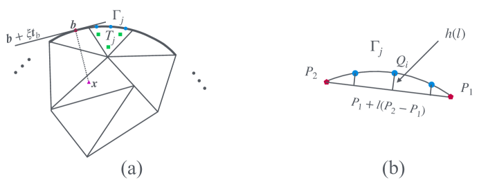
Figure 1: (a) A portion of a domain composed of triangular elements. The triangle $T_{j}$ is a boundary triangle with curved boundary segment $\Gamma_{j}$ described by at least three points (indicated by blue circles). The green squares in $T_{j}$ indicate the locations of quadrature nodes for an integration rule over the triangle. For an interior point $\bm{x}$, we denote by $\bm{b}$ the closest point on the boundary. In our asymptotic formulas, we re-express the curve and layer potential densities in terms of the parameter $\xi$, the excursion in the tangent direction $\bm{t}_{b}$. (b) Given the points defining a curved boundary segment (or chunk) $\Gamma_{j}$, we reparametrize $\Gamma_{j}$ in terms of chordal arclength $l$ $-$ that is, the distance along the chord connecting the first endpoint $P_{1}$ with the second endpoint $P_{2}$. $h(l)$ is the excursion of a boundary node $Q_{i}$ in the direction of the outward normal to the chord. When we wish to refine/oversample the user-provided chunk, we do this in the chordal parametrization by interpolating $h(l)$. The additional work is negligible and the user interface is unaffected.

$\bullet$ We assume that the domain $\Omega$ has been approximated as a union of triangles: $\Omega^{\ast}=\cup_{j=1}^{M}T_{j}$, and that each triangle $T_{j}$ is equipped with a $p$-point quadrature rule of order $q_{v}$, so that

$$\int_{T_{j}}g(\bm{x})\,\mathrm{d}\bm{x}\approx\sum_{l=1}^{p}g(\bm{x}_{l})\,w_{l}$$

for smooth functions $g(\bm{x})$. The total number of interior degrees of freedom is denoted by $N=Mp$.

$\bullet$ We will refer to the triangles whose sides form the boundary of $\Omega^{\ast}$ as boundary triangles. For each triangle segment lying on the boundary, we assume that it is described by a polynomial of degree $q_{B}$ with respect to some parametrization (see Fig. 1). For simplicity of presentation, we assume that $q_{B}\geq 2$, so that we have at least a first order accurate estimate of curvature. This requires at least $q_{B}+1$ points on each segment.

$\bullet$ We will refer to the boundary segments as chunks, and denote by $M_{B}$ the number of such chunks, so that $\Gamma^{\ast}=\partial\Omega^{\ast}=\cup_{j=1}^{M_{B}}\Gamma_{j}$. The total number of boundary degrees of freedom is $N_{B}=M_{B}(q_{B}+1)$. Note that for a reasonably uniform discretization, $N_{B}\approx\sqrt{N}$. As we shall see in Section 4.1, we will have the need to oversample each chunk on the fly. For this, we reparametrize the chunk in terms of chordal arc length as illustrated in Fig. 1.

$\bullet$ Let $\delta_{1}$ denote the local cutoff in defining $\mathcal{V}_{L}[f]$, $\mathcal{S}_{L}[\sigma]$, $\mathcal{D}_{L}[\mu]$. We assume that $\delta_{1}$ is sufficiently small that, for any interior point $\bm{x}\in\Omega$ whose distance from the boundary is less than $12\sqrt{\delta_{1}}$, there is a unique point on $\Gamma^{\ast}$ closest to $\bm{x}$. That is, $\bm{b}=\operatorname*{arg\,min}_{\bm{y}\in\Gamma^{\ast}}\|\bm{y}-\bm{x}\|_{2}$ is well-defined and unique (see Fig. 1). (The value $12\sqrt{\delta}$ is chosen because the local part of the heat kernel has decayed to less than $10^{-14}$ at that distance.) We assume the availability of a procedure to determine $\bm{b}$. In our examples, we use the closest discretization node to $\bm{x}$ as an initial guess, followed by two steps of Newton’s method to find $\bm{b}$ with high precision. Since this is a standard issue in computational geometry, independent of the solver, we omit further details (except to note that we can make use of the chordal parametrization for this).

$\bullet$ The parameter $\delta_{1}$ also controls the rate of decay of the Fourier transform for $\mathcal{V}_{NH}[f]$, $\mathcal{S}_{NH}[\sigma]$, $\mathcal{D}_{NH}[\mu]$. From the exponential decay of the integrand, once $k^{NH}_{max}$ satisfies $e^{-\left(k^{NH}_{max}\right)^{2}\delta_{1}}<\epsilon$ we have that

(32) $$\mathcal{V}_{NH}[f](\bm{x})=\int_{-k^{NH}_{max}}^{k^{NH}_{max}}\frac{e^{-\|\bm{k}\|^{2}\delta_{1}}-e^{-\|\bm{k}\|^{2}\delta_{2}}}{\|\bm{k}\|^{2}}e^{i\bm{k\cdot x}}\hat{f}(\bm{k})\,\mathrm{d}\bm{k}+O(\epsilon)\,,$$

and the same holds for $\mathcal{S}_{NH}[\sigma]$ and $\mathcal{D}_{NH}[\mu]$. (For the double layer potential, it is clear from (29) that a slightly greater cutoff is needed, namely $k^{NH}_{max}$ must satisfy $k^{NH}_{max}e^{-\left(k^{NH}_{max}\right)^{2}\delta_{1}}<\epsilon$.)

$\bullet$ The parameter $\delta_{2}$ controls the rate of decay of the Fourier transform for $\mathcal{V}_{FH}[f]$, $\mathcal{S}_{FH}[\sigma]$, $\mathcal{D}_{FH}[\mu]$. Once $k^{FH}_{max}$ satisfies $e^{-\left(k^{FH}_{max}\right)^{2}\delta_{2}}<\epsilon$, we have that

(33) $$\mathcal{V}_{FH}[f](\bm{x})=\int_{-k^{FH}_{max}}^{k^{FH}_{max}}e^{-\|\bm{k}\|^{2}\delta_{2}}\,W(\bm{k})e^{i\bm{k\cdot x}}\hat{f}(\bm{k})\,\mathrm{d}\bm{k}+O(\epsilon)\,,$$

with $W(\bm{k})$ given by (22). The same holds for $\mathcal{S}_{FH}[\sigma]$ and $\mathcal{D}_{FH}[\mu]$. (For the double layer potential, as above, a slightly greater cutoff is needed, namely $k^{FH}_{max}$ must satisfy $k^{FH}_{max}e^{-\left(k^{FH}_{max}\right)^{2}\delta_{2}}<\epsilon$.)

$\bullet$ It remains to determine the number of discretization points needed for the integrals in (32) and (33). Let us assume, without loss of generality, that the domain of interest lies in $B=[-1,1]^{2}$. For interior problems, this requires that $\Omega\subset B$. For exterior problems, this requires that $\Omega$, the support of $f(\bm{x})$, and any additional target points of interest all lie in $B$. Assuming our domain is triangulated quasi-uniformly with $N$ interior points, the average spacing between points, denoted by $\Delta x$, in either coordinate direction is of the order $O(1/\sqrt{N})$. Letting $\delta_{1}=O(1/N)$ and letting $n^{NH}_{f}$ denote the number of equispaced quadrature nodes used on $[-k^{NH}_{max},k^{NH}_{max}]$ in (32), the error decays superalgebraically with $n^{NH}_{f}$, with rapid convergence beginning when $n_{f}=O(\sqrt{N})$. Thus, the total number of discretized Fourier modes, $N_{F}=(n^{NH}_{f})^{2}$ is of the order $O(N)$. To see this, observe that the maximum excursion between a source and a target is $2$ in each dimension, so that there are at most $2k^{NH}_{max}/(2\pi)$ oscillations in the integrand and Nyquist sampling corresponds to $n^{NH}_{f}=2k^{NH}_{max}/\pi$. Since $\delta_{1}=O(1/N)=O(\Delta x^{2})$, in order to achieve a precision $\epsilon$, we must have $e^{-\left(k^{NH}_{max}\right)^{2}\delta_{1}}=\epsilon$. Combining these facts,

(34) $$n^{NH}_{f}\approx\frac{\sqrt{\log(1/\epsilon)}}{\pi}\cdot O(1/\sqrt{\delta_{1}})\approx\frac{\sqrt{\log(1/\epsilon)}}{\pi}\cdot O(\sqrt{N}).$$

Similar estimates for $n^{NH}_{f}$ hold for $\mathcal{S}_{NH}[\sigma]$ or $\mathcal{D}_{NH}[\mu]$. For the far history contribution (33), the kernel $W(\bm{k})$ introduces additional oscillations. It is straightforward to show that, for Nyquist sampling,

(35) $$n^{FH}_{f}\approx 2\sqrt{2}\,\frac{\sqrt{\log(1/\epsilon)}}{\pi}\cdot O(1/\sqrt{\delta_{2}}).$$

We omit a detailed proof and refer the interested reader to [42, 75]. Note that, once $\delta_{2}>8\delta_{1}$, the total number of Fourier modes for the far history is smaller than for the near history, despite the fact that the integrand is more oscillatory. In practice, we choose $\delta_{2}=32\delta_{1}$ for optimal performance.

3 Rapid evaluation of the near and far history

The algorithm below accounts for the near and far history from any combination of volume, single and double layer potentials using the Fourier representations from the preceding section. All computations are easily carried out using the NUFFT [11, 12, 23, 24, 29, 35, 61].

NUFFT computation of history part

Input: Suppose we are given a set of points $\bm{x}[j]$ and smooth quadrature weights $w[j]$ for $j=1,\ldots,N$ that discretize the support of $f(\bm{x})$ in the domain $\Omega$ (whether it is an interior or exterior problem). Suppose we are also given a set of points $\bm{x}_{\Gamma}[j^{\prime}]$ and weights $w_{\Gamma}[j^{\prime}]$ for $j^{\prime}=1,\ldots,N_{B}$ that discretize smooth functions restricted to the boundary $\Gamma$. Let $\delta_{1}=C\Delta x^{2}$ where $\Delta x$ is the average grid spacing in the discretization. (We typically choose $C=3$.) Let $\delta_{2}=32\,\delta_{1}$. For a tolerance $\epsilon$, compute the smallest $k^{NH}_{max}$, $k^{FH}_{max}$ such that

$$k^{NH}_{max}e^{-\left(k^{NH}_{max}\right)^{2}\delta_{1}}<\epsilon\quad,\quad k^{FH}_{max}e^{-\left(k^{FH}_{max}\right)^{2}\delta_{2}}<\epsilon.$$

Step 1: Compute $n^{NH}_{f}$ and $n^{FH}_{f}$ according to (34) and (35), to achieve about twice the Nyquist sampling frequency:

(36) $$n^{NH}_{f}\equiv\frac{2\sqrt{\log(1/\epsilon)}}{\pi\,\sqrt{\delta_{1}}}\quad,\quad n^{FH}_{f}\equiv\frac{4\sqrt{2}\sqrt{\log(1/\epsilon)}}{\pi\,\sqrt{\delta_{2}}}.$$

Let $(k^{NH}_{l,1},k^{NH}_{l,2})=\bm{k}^{NH}[l]$ denote the uniformly spaced grid points on the square $[-k^{NH}_{max},k^{NH}_{max}]^{2}$ with $n^{NH}_{f}$ points in each linear dimension. Let $N^{NH}_{f}=(n^{NH}_{f})^{2}$ denote the total number of discrete Fourier modes for the near history. Similarly, let $(k^{FH}_{l,1},k^{FH}_{l,2})=\bm{k}^{FH}[l]$ denote the uniformly spaced grid points on the square $[-k^{FH}_{max},k^{FH}_{max}]^{2}$ with $n^{FH}_{f}$ points in each linear dimension. Let $N^{FH}_{f}=(n^{FH}_{f})^{2}$ denote the total number of discrete Fourier modes for the far history.

Step 2: Compute the discrete Fourier transform

$$\hat{u}_{NH}[l]= \sum_{j=1}^{N}e^{i\bm{k}[l]\cdot\bm{x}[j]}\left(f(\bm{x}[j])w[j]\right)+$$

$$\sum_{j^{\prime}=1}^{N_{B}}e^{i\bm{k}[l]\cdot\bm{x}_{\Gamma}[j]}\left(\sigma(\bm{x}_{\Gamma}[j^{\prime}])w_{\Gamma}[j^{\prime}]\right)+$$

$$ik_{l,1} \sum_{j^{\prime}=1}^{N_{B}}e^{i\bm{k}[l]\cdot\bm{x}_{\Gamma}[j^{\prime}]}\left(\nu_{1}(\bm{x}_{\Gamma}[j^{\prime}])\mu(\bm{x}_{\Gamma}[j^{\prime}])w_{\Gamma}[j^{\prime}]\right)+$$

$$ik_{l,2} \sum_{j^{\prime}=1}^{N_{B}}e^{i\bm{k}[l]\cdot\bm{x}_{\Gamma}[j^{\prime}]}\left(\nu_{2}(\bm{x}_{\Gamma}[j^{\prime}])\mu(\bm{x}_{\Gamma}[j^{\prime}])w_{\Gamma}[j^{\prime}]\right)$$

where $\bm{k}[l]=(k_{l,1},k_{l,2})=\bm{k}^{NH}[l]$ for $l=1,\ldots,N^{NH}_{f}$.

The NUFFT computes precisely such sums, requiring $O(N_{f}\log N_{f}+N+N_{B})$ work for $N_{f}$ Fourier modes, and there are a number of open source packages for this purpose. We use the high performance FINUFFT package [11, 12].

Note that the volumetric and single layer contributions (involving $f(\bm{x})$ and $\sigma(\bm{x}_{\Gamma})$) require one NUFFT call. For the double layer potential (involving $\mu(\bm{x}_{\Gamma})$), two calls are required because the third sum involves post-multiplication with $ik_{l,1}$, and the fourth sum involves post-multiplication with $ik_{l,2}$.

Step 3: Repeat with $\bm{k}[l^{\prime}]=\bm{k}^{FH}[l^{\prime}]$ for $l^{\prime}=1,\ldots,N^{FH}_{f}$ to obtain $\hat{u}_{FH}[l^{\prime}]$.

Step 4: For every point $\bm{x}$ of interest, compute the near and far history contributions:

$$u^{NH}(\bm{x})=\sum_{l=1}^{N_{f}^{NH}}\hat{u}_{NH}[l]\left[\frac{e^{-\|\bm{k}[l]\|^{2}\delta_{1}}-e^{-\|\bm{k}[l]\|^{2}\delta_{2}}}{\|\bm{k}[l]\|^{2}}\right]e^{-i\bm{k}[l]\cdot\bm{x}}$$

where $\bm{k}[l]=\bm{k}^{NH}[l]$, and

$${u}^{FH}(\bm{x})=\sum_{l^{\prime}=1}^{N_{f}^{FH}}\hat{u}_{FH}[l^{\prime}]\,W(\bm{k}[l^{\prime}])\,e^{-i\bm{k}[l^{\prime}]\cdot\bm{x}}$$

where $\bm{k}[l^{\prime}]=\bm{k}^{FH}[l^{\prime}]$. The point $\bm{x}$ can lie anywhere in the domain $\Omega$ or on its boundary, but within the enclosing box $B$. If $N_{tot}$ denotes the total number of such target points, the cost is of the order $O\left(N_{f}^{NH}\log N_{f}^{NH}+N_{tot}\right)$ + $O\left(N_{f}^{FH}\log N_{f}^{FH}+N_{tot}\right)$ using the NUFFT.

Remark 3.1.

A simpler algorithm would be to merge the near and far history parts together, by evaluating the expression for the far history part alone with $\delta_{2}=\delta_{1}$. This, however, would require setting

$$n^{FH}_{f}\equiv\frac{4\sqrt{2}\sqrt{\log(1/\epsilon)}}{\pi\,\sqrt{\delta_{1}}},$$

with a computational cost that is approximately $8=(2\sqrt{2})^{2}$ times more expensive than the near history component above. By setting $\delta_{2}>8\delta_{1}$, the additional burden is at most a factor of two, resulting in a net speedup by a factor of 4 (as well as reduced storage requirements).

4 Rapid evaluation of local heat potentials

In this section, we present explicit asymptotic expansions for $\mathcal{S}_{L}[\sigma](\bm{x})$, $\mathcal{D}_{L}[\mu](\bm{x})$, and $\mathcal{V}_{L}[f](\bm{x})$ for orders up to $\delta^{5/2}$. Since we have fixed $\delta_{1}$ to be of the order $O(\Delta x^{2})$, these formulas yield fifth order accuracy in $\Delta x$ without additional effort. The target point $\bm{x}\in\mathbb{R}^{2}$ may either be on the boundary, in the interior of $\Omega$ or in its exterior $\Omega^{E}$. For points off boundary, as discussed in Section 2.2, we assume there is a unique closest point $\bm{b}=(b_{1},b_{2})$ on $\partial\Omega$. Letting $\bm{\nu}_{b}=\bm{\nu}(\bm{b})$ be the outward normal at $\bm{b}$, and $r=\|\bm{b}-\bm{x}\|_{2}$, we have that $\bm{x}=\bm{b}-{\rm sgn}(\bm{x})r\bm{\nu}_{b}$, where ${\rm sgn}(\bm{x})=1,0,-1$ for $\bm{x}$ in $\Omega$, $\partial\Omega$, $\Omega^{E}$, respectively.

For a given target $\bm{x}=(x_{1},x_{2})$ with closest boundary point $\bm{b}$, the asymptotic analysis is simplest in a coordinate system obtain by rotation and translation so that the tangent line at $\bm{b}$ is aligned with the $x_{1}$ direction, and translated such that: $\bm{b}$ lies at the origin for layer potentials and $\bm{x}$ lies at the origin for volume potentials. We then reparametrize the curve $\Gamma$ locally as $x_{2}=\gamma(x_{1})$ and reparametrize the densities $\sigma(\bm{x}_{\Gamma})$, $\mu(\bm{x}_{\Gamma})$ as functions along the tangent line as well (depicted in Fig. 1). More precisely, let $\sigma_{b}=\sigma(\bm{b})$ and $\mu_{b}=\mu(\bm{b})$, and denoting by $\xi$ the excursion along the tangent line, we have $x_{1}(\xi)=\xi$,

$$x_{2}(\xi) \approx\frac{1}{2}\gamma^{\prime\prime}\xi^{2}+\frac{1}{6}\gamma^{(3)}\xi^{3}+\frac{1}{24}\gamma^{(4)}\xi^{4}+\dots$$

(37) $$\sigma(\xi) \approx\sigma_{b}+\sigma_{b}^{\prime}\xi+\frac{1}{2}\sigma_{b}^{\prime\prime}\xi^{2}+\dots$$

$$\mu(\xi) \approx\mu_{b}+\mu_{b}^{\prime}\xi+\frac{1}{2}\mu_{b}^{\prime\prime}\xi^{2}+\dots$$

Note that in this parametrization, $\gamma^{\prime\prime}$ is the curvature of the boundary at $\bm{b}$. This transition is particularly simple given the chordal parametrization.

Lemma 4.1.

For $\bm{x}\in\mathbb{R}^{2}$, let $\bm{b}$ denote the closest point on the boundary $\partial\Omega$, let $c=r/\sqrt{\delta}$, and let $\kappa_{b}$ denote the curvature of the boundary at $\bm{b}$. Let $\sigma_{b}=\sigma(\bm{b})$ and let $\delta=\delta_{1}$ denote the short-time cutoff in the definition (26). Then

(38) $$\begin{split}\mathcal{S}_{L}[\sigma](\bm{x})&=\sqrt{\delta}\frac{\sigma_{b}}{2}\left(c\,\mathrm{erfc}\left(\frac{c}{2}\right)-\frac{2e^{-\frac{c^{2}}{4}}}{\sqrt{\pi}}\right)+{\rm sgn}(\bm{x})\delta\frac{c\kappa_{b}\sigma_{b}}{4}\left(c\,\mathrm{erfc}\left(\frac{c}{2}\right)-\frac{2e^{-\frac{c^{2}}{4}}}{\sqrt{\pi}}\right)\\ &+\delta^{3/2}\frac{\sigma_{b}\kappa_{b}^{2}}{12}\left(2c^{3}\mathrm{erfc}\left(\frac{c}{2}\right)-\frac{\left(4c^{2}+1\right)e^{-\frac{c^{2}}{4}}}{\sqrt{\pi}}\right)+\delta^{3/2}\frac{\sigma^{\prime\prime}_{b}}{12}\left(\frac{2\left(c^{2}-2\right)e^{-\frac{c^{2}}{4}}}{\sqrt{\pi}}-c^{3}\mathrm{erfc}\left(\frac{c}{2}\right)\right)\\ &+\delta^{2}{\rm sgn}(\bm{x})\left[\frac{c\kappa_{b}^{3}\sigma_{b}}{16}\left(3c^{3}\mathrm{erfc}\left(\frac{c}{2}\right)-\frac{\left(6c^{2}-2\right)e^{-\frac{c^{2}}{4}}}{\sqrt{\pi}}\right)+\frac{c\kappa_{b}\sigma^{\prime\prime}_{b}}{8}\left(\frac{2\left(c^{2}-2\right)e^{-\frac{c^{2}}{4}}}{\sqrt{\pi}}-c^{3}\mathrm{erfc}\left(\frac{c}{2}\right)\right)\right]\\ &+\delta^{2}{\rm sgn}(\bm{x})\left[\frac{c\sigma_{b}\gamma_{b}^{(4)}}{48}\!\left(\frac{2\left(c^{2}-2\right)e^{-\frac{c^{2}}{4}}}{\sqrt{\pi}}-c^{3}\mathrm{erfc}\left(\frac{c}{2}\right)\right)+\frac{c\sigma^{\prime}_{b}\gamma_{b}^{(3)}}{12}\!\left(e^{-\frac{c^{2}}{4}}\frac{(2c^{2}-4)}{\sqrt{\pi}}-c^{3}\mathrm{erfc}\left(\frac{c}{2}\right)\right)\right]\\ &+O\!\left(\delta^{\frac{5}{2}}\right),\end{split}$$

where $\mathrm{erf}$ denotes the error function and $\mathrm{erfc}$ denotes the complementary error function. Here, $\gamma_{b}^{(3)}$, and $\gamma_{b}^{(4)}$, denote the third and fourth derivatives of the curve $\partial\Omega$ at $\bm{b}$ with respect to the tangent line parametrization. $\sigma_{b}^{\prime}$ and $\sigma_{b}^{\prime\prime}$ are the first and second derivative of the density, also in the tangent line parametrization at $\bm{b}$.

Proof 4.2.

The formulas follow from a straightforward but tedious calculation using the change of variables $z=\sqrt{4t}$, $u=\xi/z$, and expanding all terms in (26) to sufficiently high order.

Note that $c=r/\sqrt{\delta}$ is of the order $O(1)$ even as $\delta\rightarrow 0$ at any location where the asymptotic formula will be invoked, because $\mathcal{S}_{L}[\sigma]$ has decayed to machine precision once the target point is about $12\sqrt{\delta}$ away from the boundary.

Corollary 4.3.

In the preceding lemma, when $\bm{x}\in\partial\Omega$, we have the simpler formula

(39) $$\mathcal{S}_{L}[\sigma](\bm{x})=-\sqrt{\delta}\frac{\sigma_{b}}{\sqrt{\pi}}-\delta^{\frac{3}{2}}\frac{1}{3\sqrt{\pi}}\left(\frac{\kappa_{b}^{2}\sigma_{b}}{4}+\sigma_{b}^{\prime\prime}\right)+O\!\left(\delta^{\frac{5}{2}}\right).$$

Lemma 4.4.

Under the same hypotheses as in Lemma 4.1, let $\mu_{b}=\mu(\bm{b})$, and let $\mu_{b}^{\prime}$, $\mu_{b}^{\prime\prime}$, $\mu_{b}^{(3)}$, and $\mu_{b}^{(4)}$ denote its first, second, third, and fourth derivatives in the tangent parametrization at $\bm{b}$. Then, for $\bm{x}\in\mathbb{R}^{2}$,

(40) $$\begin{split}\mathcal{D}_{L}[\mu]&(\bm{x})={\rm sgn}(\bm{x})\frac{\mu_{b}}{2}\mathrm{erfc}\left(\frac{c}{2}\right)+\sqrt{\delta}\frac{\kappa_{b}\mu_{b}}{2\sqrt{\pi}}e^{-\frac{c^{2}}{4}}+\delta\,{\rm sgn}(\bm{x})\left[\frac{3c\kappa_{b}^{2}\mu_{b}}{8\sqrt{\pi}}e^{-\frac{c^{2}}{4}}+\frac{c\mu^{\prime\prime}_{b}}{4}\left(\frac{2e^{-\frac{c^{2}}{4}}}{\sqrt{\pi}}-c\,\mathrm{erfc}\left(\frac{c}{2}\right)\right)\right]\\ &+\delta^{3/2}\frac{5\left(c^{2}-2\right)\kappa_{b}^{3}\mu_{b}}{16\sqrt{\pi}}e^{-\frac{c^{2}}{4}}+\delta^{3/2}\frac{\gamma^{(4)}_{b}\mu_{b}}{4\sqrt{\pi}}e^{-\frac{c^{2}}{4}}\\ &+\delta^{3/2}\frac{\kappa_{b}\mu^{\prime\prime}_{b}}{4}\left(\frac{2\left(c^{2}+1\right)e^{-\frac{c^{2}}{4}}}{\sqrt{\pi}}-c^{3}\mathrm{erfc}\left(\frac{c}{2}\right)\right)+\delta^{3/2}\frac{\gamma^{(3)}_{b}\mu^{\prime}_{b}}{12}\left(\frac{2e^{-\frac{c^{2}}{4}}\left(c^{2}+4\right)}{\sqrt{\pi}}-c^{3}\mathrm{erfc}\left(\frac{c}{2}\right)\right)\\ &+\delta^{2}{\rm sgn}(\bm{x})\left[\frac{35c\kappa_{b}^{4}\mu_{b}\left(c^{2}-6\right)}{128\sqrt{\pi}}e^{-\frac{c^{2}}{4}}+\frac{5c\left(\gamma^{(3)}_{b}\right)^{2}\mu_{b}}{12\sqrt{\pi}}e^{-\frac{c^{2}}{4}}+\frac{5c\kappa_{b}\gamma^{(4)}_{b}\mu_{b}}{8\sqrt{\pi}}e^{-\frac{c^{2}}{4}}\right]\\ &+\delta^{2}{\rm sgn}(\bm{x})5c\left[\frac{\kappa_{b}^{2}\mu^{\prime\prime}_{b}}{16}\left(\frac{2\left(c^{2}+1\right)e^{-\frac{c^{2}}{4}}}{\sqrt{\pi}}-c^{3}\mathrm{erfc}\left(\frac{c}{2}\right)\right)+\frac{\kappa_{b}\gamma^{(3)}_{b}\mu^{\prime}_{b}}{24}\left(\frac{2\left(c^{2}+4\right)e^{-\frac{c^{2}}{4}}}{\sqrt{\pi}}-c^{3}\mathrm{erfc}\left(\frac{c}{2}\right)\right)\right]\\ &+\delta^{2}{\rm sgn}(\bm{x})\frac{c\mu^{(4)}_{b}}{48}\left(c^{3}\mathrm{erfc}\left(\frac{c}{2}\right)-\frac{2\left(c^{2}-2\right)e^{-\frac{c^{2}}{4}}}{\sqrt{\pi}}\right)+O\!\left(\delta^{\frac{5}{2}}\right).\end{split}$$

Proof 4.5.

The formulas follow, as for the single layer case, using the change of variables $z=\sqrt{4t}$, $u=\xi/z$, expanding all terms (27) to sufficiently high order.

Corollary 4.6.

In the preceding lemma, when $\bm{x}\in\partial\Omega$, we have the simpler formula

(41) $$\mathcal{D}_{L}[\mu](\bm{x})=\sqrt{\delta}\frac{\kappa_{b}\mu_{b}}{2\sqrt{\pi}}+\delta^{\frac{3}{2}}\left(-\frac{5\kappa_{b}^{3}\mu_{b}}{8\sqrt{\pi}}+\frac{\kappa_{b}\mu_{b}^{\prime\prime}}{2\sqrt{\pi}}+\frac{2\mu_{b}^{\prime}\gamma_{b}^{(3)}}{3\sqrt{\pi}}+\frac{\mu_{b}\gamma_{b}^{(4)}}{4\sqrt{\pi}}\right)+O\!\left(\delta^{\frac{5}{2}}\right).$$

Note that

$$\lim_{r\rightarrow 0^{+}}\mathcal{D}_{L}[\mu](\bm{b}\pm r\bm{\nu}({\bm{b}}))=\mathcal{D}_{L}[\mu](\bm{b})\pm\frac{1}{2}\mu(\bm{b}).$$

That is, the jump relations for the harmonic double layer potential are manifested in the local part of the double layer heat potential.

For the volume integral, we have the following asymptotic expansion.

Lemma 4.7.

For $\bm{x}\in\Omega$, let $\bm{b}$ denote the closest point on the boundary $\partial\Omega$, let $c=r/\sqrt{\delta}$, and let $\kappa_{b}$ denote the curvature of the boundary at $\bm{b}$. Rotate and translate the domain $\Omega$ so that the $\xi$-direction lies along the tangent line at $\bm{b}$ and the $\eta$-direction is the inward normal at $\bm{b}$, with $\bm{x}$ lying at the origin. In this coordinate system, let the Taylor series for the source distribution be given by

$$f(\bm{x})=f+f_{\xi}\xi+f_{\eta}\eta+\frac{1}{2}f_{\xi\xi}\xi^{2}+f_{\xi\eta}\xi\eta+\frac{1}{2}f_{\eta\eta}\eta^{2}+\dots$$

and let $\delta=\delta_{1}$ denote the short-time cutoff in the definition (LABEL:heatdecompdefs). Then

(42) $$\begin{split}\mathcal{V}_{L}[f](\bm{x})&=\frac{\delta}{4}\left(2\mathrm{erf}\left(\frac{c}{2}\right)+\frac{2e^{-\frac{c^{2}}{4}}c}{\sqrt{\pi}}-c^{2}\mathrm{erfc}\left(\frac{c}{2}\right)+2\right)f\\ &+\delta^{3/2}\frac{\left((4-2c^{2})e^{-\frac{c^{2}}{4}}+\sqrt{\pi}c^{3}\,\mathrm{erfc}\left(\frac{c}{2}\right)\right)\left(\kappa_{b}f-2f_{\eta}\right)}{12\sqrt{\pi}}\\ &+\frac{\delta^{2}}{48}\left(\mathrm{erfc}\left(\frac{c}{2}\right)\left(4c^{4}\kappa_{b}f_{\eta}-3\left(c^{4}+4\right)f_{\eta\eta}+\left(c^{4}-12\right)f_{\xi\xi}-3c^{4}\kappa_{b}^{2}f\right)\right.\\ &\left.+\frac{2c\left(c^{2}-2\right)e^{-\frac{c^{2}}{4}}\left(-4\kappa_{b}f_{\eta}+3f_{\eta\eta}-f_{\xi\xi}+3\kappa_{b}^{2}f\right)}{\sqrt{\pi}}+24\left(f_{\xi\xi}+f_{\eta\eta}\right)\right)\\ &+O\!\left(\delta^{\frac{5}{2}}\right).\end{split}$$

Proof 4.8.

With the change of variables $z=\sqrt{4t}$, $u=\xi/z$, $v=\eta/z$, we can write the local part of the volume heat potential from (LABEL:heatdecompdefs) as

(43) $$\mathcal{V}_{L}[f](\bm{x})=\frac{1}{2\pi}\int_{0}^{\sqrt{4\delta}}\!\int_{-\infty}^{\infty}\int_{\frac{\gamma(uz)}{z}}^{\infty}\!z\,e^{-u^{2}}e^{-v^{2}}f(uz,vz)\,\mathrm{d}v\,\mathrm{d}u\,\mathrm{d}z.$$

The asymptotic expansion follows after a modest amount of algebra, using the relations

(44) $$\int_{-\infty}^{\infty}e^{-u^{2}}u^{n}\,\mathrm{d}u=\left\{\begin{array}[]{ll}\frac{(2m)!}{4^{m}m!}\sqrt{\pi}&\text{for}\ n=2m,\ m\in\mathbb{N},\\ &\\ 0&\text{for}\ n=2m+1\,,\end{array}\right.$$

and

(45) $$\int_{a}^{\infty}\!e^{-u^{2}}u^{n}\,\mathrm{d}u=\frac{1}{2}\Gamma\!\left(\frac{1+n}{2},a^{2}\right),$$

where $\Gamma(s,x)$ is the upper incomplete gamma function.

For target points $\bm{x}$ away from the boundary (at a distance greater than $12\sqrt{\delta}$), we may ignore exponentially small terms and obtain the simpler formula

(46) $$\mathcal{V}_{L}[f](\bm{x})=\delta f+\frac{\delta^{2}}{2}\left(f_{\xi\xi}+f_{\eta\eta}\right)+O\!\left(\delta^{3}\right).$$

For target points $\bm{x}$ on the boundary $\partial\Omega$, we have

(47) $$\mathcal{V}_{L}[f](\bm{x})=\frac{\delta}{2}f+\frac{\delta^{3/2}}{3\sqrt{\pi}}\left(2f_{\eta}-\kappa_{b}f\right)+\frac{\delta^{2}}{4}\left(f_{\xi\xi}+f_{\eta\eta}\right)+O\!\left(\delta^{\frac{5}{2}}\right).$$

Remark 4.9.

Asymptotic expansions of local layer heat potentials have been described in previous papers, including [37, 50, 73, 77]. Using slightly different language, they have also been used to develop high order quadrature methods based on regularized kernels combined with local correction or Richardson extrapolation (see, for example, [13, 14, 15, 21, 22] and the references therein). An important feature of all these methods, including our own, is that they address both the on-surface singular quadrature problem and the off-surface “close-to-touching” problem (that is the issue of evaluating nearly singular layer potentials) using only smooth quadrature rules. The uniform treatment of on and off-surface quadrature holds true for QBX (quadrature by expansion) [2, 10, 26, 44, 68] as well. QBX involves constructing a local expansion for a layer potential centered at a point off-surface, with a radius of convergence which reaches back to the boundary itself. It involves only smooth quadrature but with some degree of oversampling and some ill-conditioning because of the (nearby) Green’s function singularity. We should also note the method of [20] which, given accurate on-surface values, constructs an asymptotic expansion for close-to-touching points in terms of distance to the boundary.

Finally, we should observe that in two dimensions, there are numerous highly effective quadrature methods that deal with the Green’s function singularity directly, which we do not seek to review here (see [9, 18, 39, 40]). In three dimensions, however, our scheme is virtually unchanged, while direct quadrature methods are much less efficient in terms of the associated constants.

An important difference between the approach presented in this paper and earlier work (excepting [73]) is that we do not view the task as one of regularizing the singularity in the harmonic Green’s function ( $\log r$ in 2D and $1/r$ in 3D) or one of integrating it against a smooth density. Instead, we have fully switched to the heat potential formulation, involving only $C^{\infty}$ functions and the NUFFT for the history part coupled with asymptotic expansions for the local part. Those expansions are robust and stable independent of distance from the boundary. Moreover, in contrast to earlier schemes, we can easily achieve any desired accuracy by combining our asymptotic formulas with a telescoping, local quadrature, described briefly in the next section.

4.1 Computing the local part of volume and layer potentials with arbitrary precision

The scheme described in Section 4 can achieve convergence rates of up to fifth order accuracy, assuming $\delta_{1}=O(\Delta x^{2})$ and using asymptotic expansions of order $\delta_{1}^{p}$ with $p\leq{5/2}$. (We typically choose to truncated the expansions at order $\delta_{1}^{3/2}$ to avoid the need for high order derivatives of the boundary, as discussed in the examples below.) Suppose, however, that higher precision is desired in the local part. Reducing $\delta_{1}$, unfortunately, would cause the size of the Fourier transforms to increase, making the near history contribution extremely expensive. Instead, we combine two ideas from the numerical analysis of heat potentials: full product integration in time from [50] and the introduction of a second small parameter $\delta^{\ast}$ for which the asymptotic contribution is guaranteed to have the requested accuracy from [77]. We illustrate the idea using the single layer potential.

Suppose that one wishes to compute $\mathcal{S}_{L}[\sigma]$ to some precision $\epsilon<\delta_{1}^{p}$. For this, first determine the smallest $J$ such that $[\delta_{1}/(4^{J})]^{p}\leq\epsilon$, so that an asymptotic expansion with parameter $\delta^{\ast}=\delta_{1}/(4^{J})$ is sufficiently accurate. If $J=0$, then the local part is already being computed with the desired accuracy.

Otherwise, following [50, 77], write

(48) $$\mathcal{S}^{\ast}_{L}[\sigma](\bm{x}) =\int_{0}^{\delta^{\ast}}\!\int_{\partial\Omega}\frac{e^{-\|\bm{x-x^{\prime}}\|^{2}/4t}}{4\pi t}\,\sigma(\bm{x^{\prime}})\,\mathrm{ds}_{\bm{x^{\prime}}}\,\mathrm{d}t+\sum_{j=1}^{J}\int_{\delta_{1}/(4^{j})}^{\delta_{1}/(4^{j-1})}\!\int_{\partial\Omega}\frac{e^{-\|\bm{x-x^{\prime}}\|^{2}/4t}}{4\pi t}\,\sigma(\bm{x^{\prime}})\,\mathrm{ds}_{\bm{x^{\prime}}}\,\mathrm{d}t$$

$$=\int_{0}^{\delta^{\ast}}\!\int_{\partial\Omega}\frac{e^{-\|\bm{x-x^{\prime}}\|^{2}/4t}}{4\pi t}\,\sigma(\bm{x^{\prime}})\,\mathrm{ds}_{\bm{x^{\prime}}}\,\mathrm{d}t+\sum_{j=1}^{J}\int_{\partial\Omega}{\cal K}_{j}(\|\bm{x-x^{\prime}}\|^{2}/\delta_{1})\,\sigma(\bm{x^{\prime}})\,\mathrm{ds}_{\bm{x^{\prime}}}\,,$$

where the difference kernel ${\cal K}_{j}(r)$ is given by

$${\cal K}_{j}(r)=\frac{1}{4\pi}\left[E_{1}(4^{j-2}r)-E_{1}(4^{j-1}r)\right]\,$$

from (19). The first term (the integral over the interval $[0,\delta^{\ast}]$) is evaluated to the desired precision using asymptotics. Each of the terms involving difference kernels is infinitely differentiable but more sharply peaked with each refinement level. In fact, it is easy to verify that the range of the kernel to any fixed precision decreases by a factor of two when $j\rightarrow j+1$, requiring a doubling of the number of quadrature points over the range of interest. Taking the perspective of a target point $\bm{x^{\prime}}$, however, the range of non-negligible interactions has shrunk by a factor of two at the same time. Combining these facts, it is easy to see that the number of quadrature nodes that make a non-negligible contribution to a target remains the same and thus, the work for each target is constant at every level using only a smooth quadrature rule and direct summation (without the NUFFT or any other acceleration). This idea extends naturally to the double layer and volume heat potential (and is used in a slightly different form in the DMK-based box code of [42]).

Since $\sqrt{\delta_{1}}\approx\Delta x$, the telescoping series correction is entirely local for any chunk, and the only aspect of the procedure that requires some care is that each chunk should be processed independently in order to avoid excessive storage. We omit further details in the present paper for the sake of simplicity. In our third order accurate experiments on quasi-uniform triangulations, we determined that the error constants stemming from layer potential asymptotics generally exceed those from volume potential asymptotics. Thus, we apply this telescoping correction only to the local layer potentials. Carrying out three steps of dyadic refinement for $\mathcal{S}_{L}[\sigma]$ and $\mathcal{D}_{L}[\mu]$ clearly reduces the associate error constant in the layer potential part by a factor of $(1/64)^{p}$, which is more than sufficient in all of our tests. Detailed timings will be presented in Section 6.

5 The boundary integral correction

When solving an interior boundary value problem in a simply connected domain with Dirichlet conditions, standard potential theory [38, 43, 55, 69] suggests a representation for the solution $u$ of the form (9), repeated here:

$$u(\bm{x})=\mathcal{V}[f](\bm{x})+\mathcal{D}[\mu](\bm{x})\quad\text{for }\bm{x}\in\Omega.$$

Taking the limit as $\bm{x}$ approaches the boundary and using the jump relations (8), we obtain the integral equation

(49) $$-\frac{1}{2}\mu(\bm{x^{\prime}})+\mathcal{D}[\mu](\bm{x^{\prime}})=g(\bm{x^{\prime}})-\mathcal{V}[f](\bm{x^{\prime}})\quad\text{for }\bm{x^{\prime}}\in\partial\Omega.$$

When $\Omega$ is an exterior domain, in addition to the Dirichlet boundary conditions, the behavior of the solution at infinity must be specified [34, 55, 69]. More precisely, the coefficient $A$ must be given corresponding to growth at infinity of the order $A\log\|\bm{x}\|$. (Bounded solutions correspond to setting $A=0$.) A standard representation for the solution is

(50) $$u(\bm{x})=\mathcal{V}[f](\bm{x})+\mathcal{D}_{E}[\mu](\bm{x})+A\log\|\bm{x}-\bm{x}_{0}\|\quad\text{for }\bm{x}\in\Omega,$$

where $\bm{x}_{0}$ is some point in the interior of the closed curve $\partial\Omega$, and

$$\mathcal{D}_{E}[\mu](\bm{x})\equiv\int_{\partial\Omega}\left[\frac{\partial G}{\partial{\nu}_{\bm{x^{\prime}}}}(\bm{x}-\bm{x^{\prime}})+1\right]\mu(\bm{x^{\prime}})\,\mathrm{ds}_{\bm{x^{\prime}}}\quad\text{for }\bm{x}\in\Omega.$$

For the Neumann problem, with boundary condition (10), Green’s representation formula (10) leads to the integral equation

(51) $$\frac{1}{2}u(\bm{x^{\prime}})+\mathcal{D}[u](\bm{x^{\prime}})=\mathcal{V}[f](\bm{x^{\prime}})+\mathcal{S}[g](\bm{x^{\prime}})\quad\text{for }\bm{x^{\prime}}\in\partial\Omega.$$

These boundary integral equations are classical [8, 47] and there are numerous fast solvers that have been developed for their solution, described for example in the text [52]. In the present paper, we make use of GMRES iteration coupled with fast multipole acceleration [7], as in [34]. Since this is a mature subject, and we are using standard techniques, we omit further details.

6 Numerical results

We have implemented the algorithms above in Fortran 77/90, using the fmm2d library [7] combined with GMRES iteration to solve the relevant boundary integral equations and the FINUFFT library [12] to compute the nonuniform fast Fourier transforms. The timings below were obtained using an AMD Ryzen 7 PRO 6850U CPU with 16 Mb cache, with everything compiled in single-threaded mode so that we can easily compute the number of points processed per second per core (a useful figure of merit for linear or nearly linear scaling algorithms).

Given a description of the boundary $\Gamma$, we generate a curvilinear triangulation using MeshPy [45] as an interface to Triangle [66, 67]. In the interior of each triangular element, we use six Vioreanu-Rokhlin nodes [76], obtained from [46]. This is sufficient for integrating polynomials of degree two, resulting in third order accuracy. In all experiments, we generate a sequence of up to seven meshes, with

$$h\in\{0.1,0.075,0.05,0.025,0.01,0.0075,0.005\},$$

where $h$ is the length of the longest side amongst all mesh elements. Given such a triangulation with quadrature weights $w_{i},\ i=1,\dots,N$, we define $\Delta x^{2}=\frac{1}{N}\sum_{i=1}^{N}w_{i}$ and set $\delta=3\Delta x^{2}$.

In our tests, all boundary curves are assumed to take the form

(52) $$\bm{\gamma}(t)=r\left(\sum\limits_{k=0}^{N_{c}}\alpha_{k}\cos(kt)+\sum\limits_{k=1}^{N_{s}}\beta_{k}\sin(kt)\right)\begin{bmatrix}\cos(st)\\ \sin(st)\end{bmatrix}+\begin{bmatrix}x_{0}\\ y_{0}\end{bmatrix}\quad{\rm for}\ t\in[0,2\pi),$$

parametrized by $r,\{\alpha_{k}\},\{\beta_{k}\},x_{0},y_{0},s$. We set the tolerance for NUFFT to $10^{-6}$, the tolerance for GMRES to $10^{-8}$, and the tolerance for the FMM to $10^{-6}$. The tolerance $\epsilon$ for the history part (36) is also set to $10^{-6}$.

Errors are computed over all quadrature nodes in the volumetric discretization in $\ell_{\infty}$ and $\ell_{2}$ norms. Since, for interior Neumann problems, the solution is only unique up to an arbitrary constant, we define the error as

(53) $$e_{\infty}=\frac{\|(\tilde{u}-\tilde{u}_{c})-(u-u_{c})\|_{\infty}}{\|u-u_{c}\|_{\infty}},\quad e_{2}=\frac{\|(\tilde{u}-\tilde{u}_{c})-(u-u_{c})\|_{2}}{\|u-u_{c}\|_{2}},$$

where $u_{c}=u(\bm{x}_{c})$ for a randomly chosen point $\bm{x}_{c}$ and $\tilde{u}$ is our approximate computed solution. For Dirichlet boundary conditions, we may set $\tilde{u}_{c}=u_{c}=0$.

In our first experiment, we verify the convergence rates for our asymptotic expansions. Our second example is an interior Neumann problem and our third example is an exterior Dirichlet problem. For our last example, we study the effect of poor mesh quality (degenerate triangles, high aspect ratio elements and gaps) in the solution of an interior Dirichlet problem.

6.1 Validation of high order asymptotic expansions

For the single and double layer potentials, we consider the domain $\Omega$ with boundary given by Eq. 52, with nonzero parameters $r=1$, $\alpha_{0}=5/6$, $\beta_{3}=1/30$, $\alpha_{5}=1/15$, $\alpha_{6}=1/30$, $\alpha_{8}=1/30$, $\alpha_{10}=1/30$, and $s=1$. (See Fig. 3.) We assume the layer potential densities are given by

$$\sigma(t)=\mu(t)=1+\sin(2t)+\cos(4t)\quad\text{for }t\in[0,2\pi).$$

We measure the error in evaluating $\mathcal{S}_{L}[\sigma]$ and $\mathcal{D}_{L}[\mu]$ at $10000$ random locations in the box $[-1,1]^{2}$, which entirely contains $\bar{\Omega}$. All curve and density derivatives that appear in the asymptotic formulas are computed analytically. We also use a sixteenth order discretization of the boundary $\partial\Omega$, and set all tolerances to fourteen digits of accuracy in order to ensure that errors are due exclusively to the asymptotic approximations. The results are shown in the left and center panels of Fig. 2, where we observe the expected order of convergence from Eq. 38 and Eq. 40.

(a)

(b)

(c)

Figure 2: Relative errors as functions of $\delta$ for $\mathcal{S}_{L}[\sigma]$ (left), $\mathcal{D}_{L}[\mu]$ (center) and $\mathcal{V}_{L}[f]$ (right) using asymptotic expansions of order $O\!\left(\delta^{p/2}\right)$ with $p=4,5$. Solid lines with solid markers are the relative $\ell_{\infty}$ errors, dotted lines with open markers are the relative $\ell_{2}$ errors. Square markers (${\blacksquare}$, ${\square}$) correspond to $p=4$, while round markers ($\bullet$, $\circ$) correspond to $p=5$. The dashed and dot-dash lines, without markers, are reference curves with convergence rate $\delta^{p/2}$ for $p=4,5$, respectively.

For the volume potential, we solve the interior Dirichlet problem in the same domain $\Omega$ with volumetric data

(54) $$f(\bm{x})=-50\sin(5(x_{1}+x_{2}))+2/9+1000(1000x_{1}^{2}-1)e^{-500x_{1}^{2}}\quad\text{for }\bm{x}\in\Omega.$$

The volume potential $\mathcal{V}[f](\bm{x})$ is computed using the near and far history and $\mathcal{V}_{L}[f](\bm{x})$ on a sequence of seven meshes as indicated above. In order to make the double layer potential error negligible, we use the technique described in [40] with sixteenth order accuracy. The errors are computed at $5000$ random points in $\Omega$ and the results plotted in Fig. 2 (right panel), where we observe the expected orders of convergence from Eq. 42 in the errors as functions of $\delta$.

6.2 An interior Neumann problem

For the same domain, we consider the exact solution

(55) $$u(\bm{x})=\frac{(x_{1}-a)}{(x_{1}-a)^{2}+(x_{2}-b)^{2}}+\frac{x_{1}^{2}}{9}-x_{2}+8+e^{-5x_{1}^{2}}+u_{c}\quad\text{for }\bm{x}\in\Omega,$$

where $u_{c}$ is an additive constant, $a=1.1$, and $b=1.3$.

The function $u(\bm{x})$ satisfies the Poisson equation with source density

(56) $$f(\bm{x})=\frac{2}{9}+(100x_{1}^{2}-10)e^{-5x_{1}^{2}}\quad\text{for }\bm{x}\in\Omega,$$

and we may compute the Neumann boundary data $g(\bm{x})=\bm{\nu}(\bm{x})\cdot\nabla u(\bm{x})$ analytically.

In Fig. 3, we show a quasi-uniform mesh on $\Omega$ for $h\approx 0.1$ together with a plot of the solution $u$, given by Eq. 55 with $u_{c}=0$.

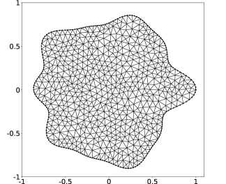
(a)

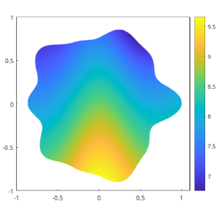
(b)

Figure 3: A volumetric mesh for the domain $\Omega$ in Section 6.2 (left). There are $1142$ triangles in the discretization, with $h\approx 0.1$ and $208$ nodes along the boundary $\partial\Omega$, marked with black dots. The solution to the interior Neumann problem Eq. 55, with $u_{c}=0$ is plotted on the right.

We solve the interior Neumann problem for a sequence of seven meshes, using three levels of dyadic refinement to improve the accuracy of the local parts of the layer potentials, as described in Section 4.1. In the asymptotic formulas, we include terms up to $O(\delta)$. The resulting errors are of the order $O\!\left(\delta^{3/2}\right)$, which is equivalent to third order accuracy with respect to $\Delta x$.

The errors in the approximate solutions are plotted in Fig. 4 (left panel) as functions of $\Delta x$. The convergence rate is clearly third order, until about five digits of accuracy are obtained. (The reader may note that the prescribed tolerances were set to six digits of accuracy. We lose one digit of accuracy due to the indeterminacy of the Neumann problem. Our computed solution happened to be ten times larger than the exact solution with $u_{c}=0$.) In Fig. 4 (right panel) we plot the total time for solving and evaluating the solution at all interior nodes. These timings do not include mesh generation, but include all other steps for solving the Poisson equation. For $N_{V}=674664$, $1198728$, $2695248$ (the three rightmost data points), the throughput is $8.3\times 10^{5}$, $8.7\times 10^{5}$, and $8.4\times 10^{5}$ points per second per core. For problem sizes in this range, about 80% of the time is spent in evaluating $\mathcal{V}_{NH}[f]$,$\mathcal{V}_{FH}[f],\mathcal{D}_{NH}[\mu],$ and $\mathcal{D}_{FH}[\mu]$. About 10% of the time is spent in the dyadic refinement scheme of Section 4.1 and another 10% of the time is spent solving the boundary integral equation. The cost of evaluating the asymptotic expansions is negligible.

(a)

(b)

Figure 4: For the Neumann problem in Section 6.2, the left-hand plot shows the relative $\ell_{\infty}$ error (solid line with solid markers) and the relative $\ell_{2}$ error (dotted line with open markers) using our solver. The dashed line is for reference, with slope corresponding to a convergence of order $O\!\left(\Delta x^{3}\right)$. The right-hand plot shows the total time for all steps (excluding mesh generation) for solving and evaluating the solution at all volumetric quadrature nodes.

6.3 An exterior Dirichlet problem

In our next example, we let $\partial\Omega$ be defined by Eq. 52, with nonzero coefficients $r=1$, $\alpha_{0}=1$, $\alpha_{5}=3/10$, and $s=1$. (See Fig. 5.)

In $\mathbb{R}^{2}\setminus\bar{\Omega}$, we let the source density be given by

(57) $$f(\bm{x})=4\sum\limits_{i=1}^{3}e^{-\frac{(x_{1}-a_{i})^{2}+(x_{2}-b_{i})^{2}}{\sigma_{i}}}\left(\frac{(x_{1}-a_{i})^{2}+(x_{2}-b_{i})^{2}}{\sigma_{i}^{2}}-\frac{4}{\sigma_{i}}\right),$$

with $a_{1}=1/2$, $b_{1}=-1/2$, $\sigma_{1}=1/20$, $a_{2}=1/2$, $b_{2}=1/2$, $\sigma_{2}=1/40$, $a_{3}=-3/10$, $b_{3}=0$, and $\sigma_{3}=1/15$. On the boundary we assume $u(\bm{x})=g(\bm{x})$, corresponding to the exact solution

(58) $$u(\bm{x})=\sum\limits_{i=1}^{3}e^{-\frac{(x_{1}-a_{i})^{2}+(x_{2}-b_{i})^{2}}{\sigma_{i}}}+10\log((x_{1}-a_{4})^{2}+(x_{2}-b_{4})^{2})\,,$$

with $a_{4}=3/10$, and $b_{4}=-0.5$. Following the discussion in Section 5, we represent the solution as

$$u(\bm{x})=\mathcal{V}[f](\bm{x})+\mathcal{D}_{E}[\mu](\bm{x})+20\log\|\bm{x}\|\quad\text{for }\bm{x}\in\mathbb{R}^{2}\setminus\bar{\Omega}.$$

The source term is exponentially decaying, and it is easy to check that $|f(\bm{x})|<10^{-16}$ for $\bm{x}$ outside the domain $D=[-1.95,1.95]^{2}\,\setminus\bar{\Omega}$, shown in Fig. 5.

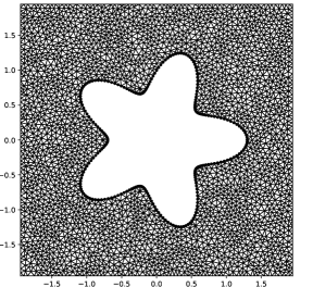
(a)

(b)

Figure 5: A volumetric mesh for the domain $D$ (left) in Section 6.3, with $36318$ elements and $h\approx 0.1$. There are $228$ nodes along the boundary $\partial\Omega$, marked with black dots. The right-hand figure shows the modulus of the source density Eq. 57 on a logartihmic scale (base 10).

We solve the exterior Dirichlet problem with six different meshes, corresponding to $h=0.1$, $0.075$, $0.05$, $0.025$, $0.01$, $0.0075$, using three levels of dyadic refinement to improve the accuracy of the local parts of the layer potentials, as described in Section 4.1. Keeping terms up to $O(\delta)$ in the asymptotic expansions, we expect third order accuracy in $\Delta x$. This is verified in Fig. 6. The $l_{\infty}$ error saturates at about $3\times 10^{-6}$, which is more or less the requested tolerance.

Note from Fig. 6 that the solver operates at about one million points per second per core for the four rightmost data points: $9.6\times 10^{5}$ for $N_{V}=146136$, $1.1\times 10^{6}$ for $N_{V}=583962$, $1.1\times 10^{6}$ for $N_{V}=3657276$, and $9.9\times 10^{5}$ for $N_{V}=6491154$.

(a)

(b)

Figure 6: For the exterior Dirichlet problem in Section 6.3, the left-hand plot shows the relative $\ell_{\infty}$ error (solid line with solid markers) and the relative $\ell_{2}$ error (dotted line with open markers). The dashed line is for reference, with slope corresponding to a convergence rate of order $O\!\left(\Delta x^{3}\right)$. The right-hand plot shows the total time for all steps (excluding mesh generation) for solving and evaluating the solution at all volumetric quadrature nodes.

6.4 Robustness With Respect to Mesh Quality

A major advantage of potential theory in solving the Poisson equation is that the volume integral $\mathcal{V}[f]$ expresses a particular solution by quadrature. This leads to both robust performance and straightforward error analysis. To see this, let $\tilde{f}(\bm{x})$ be a piecewise polynomial approximation of ${f}(\bm{x})$ and let ${\tilde{Q}}[\tilde{f}](\bm{x})$ denote the quadrature approximation of $\mathcal{V}[\tilde{f}](\bm{x})$. Then, as noted in [48], the total error can be written as

(59) $$e(\bm{x}) =|\mathcal{V}[f](\bm{x})-{\tilde{Q}}[\tilde{f}](\bm{x})|$$

$$\leq\left|\int\limits_{\Omega}G(\bm{x}-\bm{x^{\prime}})(f(\bm{x^{\prime}})-\tilde{f}(\bm{x^{\prime}}))\,\mathrm{d}\bm{x^{\prime}}\right|+\left|\int\limits_{\Omega}G(\bm{x}-\bm{x^{\prime}})\tilde{f}(\bm{x})\,\mathrm{d}\bm{x^{\prime}}-{\tilde{Q}}[\tilde{f}](\bm{x})\right|$$

$$=O(\|f(\bm{x})-\tilde{f}(\bm{x})\|_{\infty})+O(\epsilon)\,.$$

The first term in this estimate is the error in the approximation of the source distribution, and follows immediately from the fact that $\mathcal{V}$ is a bounded operator. The second term represents the quadrature error in evaluating the volume integral for the approximate right-hand side $\tilde{f}(\bm{x})$. PDE-based methods require much more complicated estimates that depend on the smoothness of the (unknown) solution itself.

As a demonstration, consider the interior Dirichlet problem in the domain $\Omega$ from Section 6.3. The source density is given by Eq. 56, and the Dirichlet boundary data by Eq. 55. We solve the problem for two sequences of mesh refinement: the first consists of seven meshes, as described in the beginning of Section 6. In the second case, we repeat the refinement process but, for every triangle, we pick one of the three sides, say $S$ at random, excluding the curved boundary segments, and pick a point $P$ at random along the line containing $S$. If $P$ ends up outside the triangle, we move it to the closest endpoint of $S$. We then split the triangle along the line drawn from the random point to the corner opposite $S$. This results in a nonconforming mesh, with elements of arbitrarily poor aspect ratio, of which about $4\%$ are actually degenerate (see Fig. 7 for an example corresponding to $h=0.1$). We use the same relation between $\delta$ and the average mesh spacing $\Delta x^{2}$ as in our other examples.

Figure 7: Left: A degenerate mesh (left) obtained from the conforming triangulation created by Triangle [66, 67] with $h=0.1$. The parametrization of the boundary is given in Section 6.3. Of the $3624$ new triangles, $127$ are degenerate. A blow-up of a small region is shown on the right.

We observe in Fig. 8 that mesh distortion had a negligible effect on the error in the solution. Moreover, removing triangles (creating gaps in the discretization) induces a small error as well $-$ proportional to the area fraction of triangles removed.

Figure 8: Relative errors, as functions of $\delta$ for numerical experiments in Section 6.4: solid lines with solid markers are the relative $\ell_{\infty}$ errors, dotted lines with open markers are the relative $\ell_{2}$ errors. Round markers ($\bullet$, $\circ$) correspond to errors for the nondegenerate meshes. Square markers (${\blacksquare}$, ${\square}$) correspond to errors for the degenerate meshes. The dashed line without markers is a reference for the expected order of convergence $O\!\left(\delta^{3/2}\right)$.

7 Discussion

We have presented a new class of fast algorithms for harmonic volume and layer potentials that is based on evaluating heat potentials to a steady state limit, separating the calculation into a “ far history” part, a “near history” part and a “local” part. The first two are evaluated using the NUFFT and the latter is computed using asymptotics (or more precisely, a combination of asymptotics and a telescoping localized quadrature rule). For layer potentials, it is closely related to the method of [37, 73] and to Ewald-like methods, which split the harmonic Green’s function into a regularized far-field kernel with a near field correction [1, 13, 14, 15, 21, 22, 37, 42, 50, 57, 64, 73].

Three novel features have been introduced here:

1. the construction of accurate asymptotic expansions for volume potentials when the volumetric source distribution is smooth within a domain $\Omega$, but discontinuous as a function in the ambient space (here $\mathbb{R}^{2}$),

2. the introduction of several steps of dyadic refinement to obtain arbitrary precision in evaluating the local part,

3. the separation of the history part into the “near” and “far” components which provides approximately a three fold speedup in the NUFFT computations (used also in [42]).

The second feature is of significant practical importance, since high order asymptotic formulas become more and more ill-conditioned, as they involve higher derivatives of the density or the curve itself (with catastrophic cancellation reducing their effectiveness). In practice, we recommend using the formulas of order no greater than $O(\delta^{3/2})$. Thus, when higher precision is requested, it is critical to be able to carry out $j$ refinement steps to make the value $\delta^{\ast}=\delta/(4^{j})$ sufficiently small before invoking the asymptotic approximation. This is described in Section 4.1 and related to the hybrid asymptotic/numerical quadrature method of [77].

From a user’s perspective, perhaps the most important feature of the method is the extent to which it is agnostic to the details of the underlying discretization. All that we require is the set of weights and nodes for a smooth quadrature rule in the domain and the set of weights and nodes for a smooth quadrature rule on the boundary. This is compatible with unstructured triangulations, adaptive quad and octtrees, spectral elements, and various kinds of composite grids [4, 5, 16, 41, 70, 63]. As demonstrated in our numerical examples, the integral formulation helps make it insensitive to flaws in the triangulation, including outright degeneracies and gaps, while maintaining extremely high throughput.

Of potential mathematical interest is that, by taking the heat potential viewpoint, our asymptotic formulas can be used to derive the jump properties of the corresponding elliptic layer potentials across the boundary quite naturally (as seen in (40) and (41)). This provides an alternative derivation to the ones typically found in the literature [38, 43, 47, 55, 69].

The algorithm presented above is suitable only for quasi-uniform triangulations, as it relies on the NUFFT for speed, and the balance between the history and local parts would be broken by multiscale triangulation. Fortunately, the tools developed here, including asymptotics and local dyadic refinement, can be integrated naturally into the DMK framework of [42] to develop a fully adaptive algorithm. We will report on that implementation, the extension to other Green’s functions, as well as three-dimensional experiments, at a later date.

8 Acknowledgements

The authors would like to thank Fabrizio Falasca at the Courant Institute of Mathematical Sciences, New York University, and Manas Rachh and Dan Fortunato at the Center for Computational Mathematics, Flatiron Institute, for helpful discussions. The first author gratefully acknowledges support from the Knut and Alice Wallenberg Foundation under grant 2020.0258. The work of the second and fourth authors was partially supported by the Office of Naval Research under award N00014-18-1-2307.

References

• [1] L. af Klinteberg, D. S. Shamshirgar, and A.-K. Tornberg, Fast Ewald summation for free-space Stokes potentials, Res. Math. Sci., 4 (2017), p. 1.
• [2] L. af Klinteberg and A.-K. Tornberg, Adaptive quadrature by expansion for layer potential evaluation in two dimensions, SIAM Journal on Scientific Computing, 40 (2018), pp. A1225–A1249.
• [3] T. G. Anderson, M. Bonnet, L. M. Faria, and C. Pérez-Arancibia, Fast, high-order numerical evaluation of volume potentials via polynomial density interpolation, J. Comput. Phys., 511 (2024), p. 113091.
• [4] T. G. Anderson, H. Zhu, and S. Veerapaneni, A fast, high-order scheme for evaluating volume potentials on complex 2D geometries via area-to-line integral conversion and domain mappings, J. Comput. Phys., 472 (2023), p. 111688.
• [5] D. Appelö, J. W. Banks, W. D. Henshaw, and D. W. Schwendeman, Numerical methods for solid mechanics on overlapping grids: Linear elasticity, J. Comput. Phys., 231 (2012), pp. 6012–6050.
• [6] T. Askham and A. J. Cerfon, An adaptive fast multipole accelerated Poisson solver for complex geometries, J. Comput. Phys., 344 (2017), pp. 1–22.
• [7] T. Askham, Z. Gimbutas, L. Greengard, L. Lu, M. O’Neil, M. Rachh, and V. Rokhlin, fmm2d software library. https://github.com/flatironinstitute/fmm2d, 2021.
• [8] K. E. Atkinson, The Numerical Solution of Integral Equations of the Second Kind, Cambridge Monographs on Applied and Computational Mathematics, Cambridge University Press, 1997.
• [9] A. Barnett, B. Wu, and S. Veerapaneni, Spectrally accurate quadratures for evaluation of layer potentials close to the boundary for the 2D Stokes and Laplace equations, SIAM Journal on Scientific Computing, 37 (2015), pp. B519–B542.
• [10] A. H. Barnett, Evaluation of layer potentials close to the boundary for Laplace and Helmholtz problems on analytic planar domains, SIAM Journal on Scientific Computing, 36 (2014), pp. A427–A451.
• [11] A. H. Barnett, J. F. Magland, and L. af Klinteberg, A parallel non-uniform fast Fourier transform library based on an “exponential of semicircle” kernel, SIAM J. Sci. Comput., 41 (2019), pp. C479–C504.
• [12] A. H. Barnett and J. F. Magland et al., Non-uniform fast Fourier transform library of types $1$, $2$, $3$ in dimensions $1$, $2$, $3$, 2018.
• [13] J. Beale, M. Storm, and S. Tlupova, The adjoint double layer potential on smooth surfaces in $\mathbb{R}^{3}$ and the Neumann problem, Adv. Comput. Math., 50 (2024), p. 29.
• [14] J. Beale and S. Tlupova, Extrapolated regularization of nearly singular integrals on surfaces, Adv. Comput. Math., 50 (2024), p. 61.
• [15] J. Beale, W. Ying, and J. Wilson, A simple method for computing singular or nearly singular integrals on closed surfaces, Commun. Comput. Phys., 20 (2016), pp. 733–753.
• [16] M. Berger, Chapter 1 - cut cells: Meshes and solvers, in Handbook of Numerical Methods for Hyperbolic Problems, R. Abgrall and C.-W. Shu, eds., vol. 18 of Handbook of Numerical Analysis, Elsevier, 2017, pp. 1–22.
• [17] A. Brandt and A. Lubrecht, Multilevel matrix multiplication and fast solution of integral equations, Journal of Computational Physics, 90 (1990), pp. 348–370.
• [18] J. Bremer, Z. Gimbutas, and V. Rokhlin, A nonlinear optimization procedure for generalized Gaussian quadratures, SIAM J. Sci. Comput., 32 (2010), pp. 1761–1788.
• [19] O. P. Bruno and J. Paul, Two-dimensional Fourier continuation and applications, SIAM Journal on Scientific Computing, 44 (2022), pp. A964–A992.
• [20] C. Carvalho, S. Khatri, and A. D. Kim, Asymptotic analysis for close evaluation of layer potentials, Journal of Computational Physics, 355 (2018), pp. 327–341.
• [21] R. Cortez, The Method of Regularized Stokeslets, SIAM Journal on Scientific Computing, 23 (2001), pp. 1204–1225.
• [22] R. Cortez, L. Fauci, and A. Medovikov, The method of regularized Stokeslets in three dimensions: Analysis, validation, and application to helical swimming, Physics of Fluids, 17 (2005), p. 031504.
• [23] A. Dutt and V. Rokhlin, Fast Fourier transforms for nonequispaced data, SIAM J. Sci. Comput., 14 (1993), pp. 1368–1393.
• [24]  , Fast Fourier transforms for nonequispaced data. II, Appl. Comput. Harmon. Anal., 2 (1995), pp. 85–100.
• [25] C. L. Epstein, F. Fryklund, and S. Jiang, An accurate and efficient scheme for function extensions on smooth domains, arXiv preprint arXiv:2206.11318, (2023).
• [26] C. L. Epstein, A. Klöckner, and L. Greengard, On the Convergence of Local Expansions of Layer Potentials, SIAM J. Num. Anal., 51 (2013), pp. 2660–2679.
• [27] F. Ethridge and L. Greengard, A new fast-multipole accelerated Poisson solver in two dimensions, SIAM J. Sci. Comput., 23 (2002), pp. 741–760.
• [28] P. Ewald, Die Berechnung optischer und elektrostatischer Gitterpotentiale, Annalen der Physik, 64 (1921), pp. 253–287.
• [29] J. A. Fessler and B. P. Sutton, Nonuniform fast Fourier transforms using minmax interpolation, IEEE Trans. Signal Proc., 51 (2003), pp. 560–574.
• [30] A. Friedman, Partial Differential Equations of Parabolic Type, Prentice-Hall, Englewood Cliffs, New Jersey, 1964.
• [31] F. Fryklund and L. Greengard, An FMM accelerated Poisson solver for complicated geometries in the plane using function extension, SIAM J. Sci. Comput., 45 (2023), pp. A3001–A3019.
• [32] F. Fryklund, M. C. A. Kropinski, and A.-K. Tornberg, An integral equation-based numerical method for the forced heat equation on complex domains, Adv. Comput. Math, 46 (2020), pp. 1–36.
• [33] F. Fryklund, E. Lehto, and A.-K. Tornberg, Partition of unity extension of functions on complex domains, J. Comput. Phys., 375 (2018), pp. 57–79.
• [34] A. Greenbaum, L. Greengard, and G. McFadden, Laplace’s equation and the Dirichlet-Neumann map in multiply connected domains, J. Comput. Phys., 105 (1993), pp. 267–278.
• [35] L. Greengard and J. Lee, Accelerating the nonuniform fast Fourier transform, SIAM Rev., 46 (2004), pp. 443–454.
• [36] L. Greengard and J.-Y. Lee, A direct adaptive Poisson solver of arbitrary order accuracy, Journal of Computational Physics, 125 (1996), pp. 415–424.
• [37] L. Greengard and J. Strain, A fast algorithm for the evaluation of heat potentials, Comm. on Pure and Appl. Math, 43 (1990), pp. 949–963.
• [38] R. B. Guenther and J. W. Lee, Partial Differential Equations of Mathematical Physics and Integral Equations, Prentice Hall, 1988.
• [39] S. Hao, A. H. Barnett, P.-G. Martinsson, and P. Young, High-order accurate methods for Nyström discretization of integral equations on smooth curves in the plane, Advances in Computational Mathematics, 40 (2014), pp. 245–272.
• [40] J. Helsing and R. Ojala, On the evaluation of layer potentials close to their sources, J. Comput. Phys., 227 (2008), pp. 2899–2921.
• [41] W. D. Henshaw, D. W. Schwendeman, J. W. Banks, and K. K. Chand, Overture. https://www.overtureframework.org/.
• [42] S. Jiang and L. Greengard, A dual-space multilevel kernel-splitting framework for discrete and continuous convolution, arXiv preprint arXiv:2308.00292, (2023).
• [43] O. D. Kellogg, Foundations of Potential Theory, Springer, 1929.
• [44] A. Klöckner, A. Barnett, L. Greengard, and M. O’Neil, Quadrature by expansion: A new method for the evaluation of layer potentials, Journal of Computational Physics, 252 (2013), pp. 332–349.
• [45] A. Klöckner, L. Brun, B. Liu, S. Klemenc, A. Fkikl, C. Gohlke, E. Coon, G. Oxberry, J. Veselý, M. Wala, M. Smith, P. Potrowl, and A. Kurtz, MeshPy. https://github.com/inducer/meshpy, 2022-11-06.
• [46] A. Klöckner, A. Fikl, X. Wei, T. Gibson, A. Alvey-Blanco, and M. Wala, ModePy. https://github.com/inducer/modepy, 2024-05-02.
• [47] R. Kress, Linear Integral Equations, vol. 82 of Applied Mathematical Sciences, Springer–Verlag, Berlin, third ed., 2014.
• [48] H. M. Langston, L. Greengard, and D. Zorin, A free-space adaptive FMM-based PDE solver in three dimensions, Commun. Appl. Math. Comput. Sci., 6 (2011), pp. 79–122.
• [49] R. J. LeVeque and Z. Li, The immersed interface method for elliptic equations with discontinuous coefficients and singular sources, SIAM Journal on Numerical Analysis, 31 (1994), pp. 1019–1044.
• [50] J. R. Li and L. Greengard, High order accurate methods for the evaluation of layer heat potentials, SIAM J. Sci. Comput., 31 (2009), pp. 3847–3860.
• [51] D. Malhotra and G. Biros, PVFMM: A parallel kernel independent FMM for particle and volume potentials, Commun. Comput. Phys., 18 (2015), p. 808–830.
• [52] P.-G. Martinsson, Fast direct solvers for elliptic PDEs, SIAM, 2019.
• [53] A. Mayo, The rapid evaluation of volume integrals of potential thory on general regions, J. Comput. Phys., 100 (1992), pp. 236–245.
• [54] A. McKenney, L. Greengard, and A. Mayo, A fast Poisson solver for complex geometries, Journal of Computational Physics, 118 (1995), pp. 348–355.
• [55] S. G. Mikhlin, Integral Equations, Pergammon, 1957.
• [56] F. W. J. Olver, D. W. Lozier, R. F. Boisvert, and C. W. Clark, eds., NIST Handbook of Mathematical Functions, Cambridge University Press, May 2010.
• [57] S. Plsson and A.-K. Tornberg, An integral equation method for closely interacting surfactant-covered droplets in wall-confined Stokes flow, International Journal for Numerical Methods in Fluids, 92 (2020), pp. 1975–2008.
• [58] P. W. Partridge, C. A. Brebbia, and L. W. Wrobel, The Dual Reciprocity Boundary Element Method, Springer, Berlin, 1992.
• [59] C. S. Peskin, The immersed boundary method, Acta Numerica, 11 (2002), p. 479–517.
• [60] W. Pogorzelski, Integral equations and their applications, Pergamon Press, Oxford, 1966.
• [61] D. Potts, G. Steidl, and A. Nieslony, Fast convolution with radial kernels at nonequispaced knots, Numer. Math., 98 (2004), pp. 329–351.
• [62] G. Russo and J. Strain, Fast triangulated vortex methods for the 2D Euler equations, J. Comput. Phys., 111 (1994), pp. 291–323.
• [63] R. I. Saye, High-order quadrature methods for implicitly defined surfaces and volumes in hyperrectangles, SIAM J. Sci. Comput., 37 (2015), pp. A993–A1019.
• [64] D. S. Shamshirgar, J. Bagge, and A.-K. Tornberg, Fast Ewald summation for electrostatic potentials with arbitrary periodicity, The Journal of Chemical Physics, 154 (2021), p. 164109.
• [65] Z. Shen and K. Serkh, Rapid evaluation of Newtonian potentials on planar domains, SIAM J. Sci. Comput., 46 (2024), pp. A609–A628.
• [66] J. R. Shewchuk, Triangle: Engineering a 2D quality mesh generator and Delaunay triangulator, in Applied Computational Geometry Towards Geometric Engineering, M. C. Lin and D. Manocha, eds., Berlin, Heidelberg, 1996, Springer Berlin Heidelberg, pp. 203–222.
• [67] J. R. Shewchuk, Triangle. https://www.cs.cmu.edu/~quake/triangle.html, 2005-07-28.
• [68] M. Siegel and A.-K. Tornberg, A local target specific quadrature by expansion method for evaluation of layer potentials in 3D, J. Comput. Phys., 364 (2018), pp. 365–392.
• [69] I. Stakgold, Boundary value problems of mathematical physics, Macmillan, 1968.
• [70] D. B. Stein, Spectrally accurate solutions to inhomogeneous elliptic PDE in smooth geometries using function intension, J. Comput. Phys., 470 (2022), p. 111594.
• [71] D. B. Stein, R. D. Guy, and B. Thomases, Immersed boundary smooth extension: A high-order method for solving PDE on arbitrary smooth domains using Fourier spectral methods, Journal of Computational Physics, 304 (2016), pp. 252–274.
• [72]  , Immersed boundary smooth extension (IBSE): A high-order method for solving incompressible flows in arbitrary smooth domains, J. Comput. Phys., 335 (2017), pp. 155–178.
• [73] J. Strain, Fast potential theory. II. layer potentials and discrete sums, J. Comput. Phys., 99 (1992), pp. 251–270.
• [74] L. N. Trefethen and J. A. C. Weideman, The exponentially convergent trapezoidal rule, SIAM review, 56 (2014), pp. 385–458.
• [75] F. Vico, L. Greengard, and M. Ferrando, Fast convolution with free-space Green’s functions, J. Comput. Phys., 323 (2016), pp. 191–203.
• [76] B. Vioreanu and V. Rokhlin, Spectra of multiplication operators as a numerical tool, SIAM J. Sci. Comput., 36 (2014), pp. A267–A288.
• [77] J. Wang and L. Greengard, Hybrid asymptotic/numerical methods for the evaluation of layer heat potentials in two dimensions, Advances in Computational Mathematics, 45 (2019), pp. 847–867.