Signature matrices of membranes

Abstract

We prove that, unlike in the case of paths, the signature matrix of a membrane does not satisfy any algebraic relations. We derive novel closed-form expressions for the signatures of polynomial membranes and piecewise bilinear interpolations for arbitrary $2$-parameter data in $d$-dimensional space. We show that these two families of membranes admit the same set of signature matrices and scrutinize the corresponding affine variety.

Keywords: two-parameter signatures, affine algebraic varieties, matrix congruence, geometry of paths and membranes, iterated integrals

MSC codes: 60L10, 14Q15, 13P25

1 Introduction

The signature of a path.

A path is a continuous map $X:[0,1]\to\mathbb{R}^{d}$ with piecewise continuously differentiable coordinate functions. Its $k$-th level signature $\sigma^{(k)}(X)$, as introduced by Chen in the seminal work [8], is a $k$-tensor of format $d\times\dots\times d$, defined by forming certain iterated integrals. In particular, its second level signature can be viewed as a signature matrix. It is defined as follows:

$$\sigma^{(2)}(X)_{i,j} :=\int_{0}^{1}\int_{0}^{t_{2}}\partial X_{i}(t_{1})\,\partial X_{j}(t_{2})\;\mathrm{d}t_{1}\mathrm{d}t_{2}$$ (1)

These matrices were studied in [2]. They satisfy some interesting properties: for example, their symmetric part has always rank $1$, due to the shuffle relations satisfied by path signatures.

Moreover, the set of signature matrices of polynomial paths with degree $\leq m$ and the set of signature matrices of piecewise linear paths with at most $m$ segments agree. The equations that vanish on these sets, that is, the varieties of signature matrices, are well-understood: they can be described as certain determinantal varieties [2, Theorem 3.4].

The signature of a membrane.

A membrane is a continuous map $X:[0,1]^{2}\rightarrow{\mathbb{R}}^{d}$ where the coordinate functions $X_{1},X_{2},\dots,X_{d}$ are (piecewise) continuously differentiable functions in the two arguments. In particular the differentials $\partial_{12}X_{j}(s,t):=\frac{\partial^{2}}{\partial s\partial t}X_{j}(s,t)$ obey the usual rules of calculus. Generalizing the path setting, one can associate a collection of tensors to $X$ via iterated integrals (see Definition 2.2). In particular, the signature matrix of a membrane $X$ is defined as an $\mathbb{R}$-valued $d\times d$-matrix with entries

$$\sigma^{(2)}(X)_{i,j} :=\int_{0}^{1}\int_{0}^{1}\int_{0}^{t_{2}}\int_{0}^{s_{2}}\partial_{12}X_{i}(s_{1},t_{1})\,\partial_{12}X_{j}(s_{2},t_{2})\;\mathrm{d}s_{1}\mathrm{d}t_{1}\mathrm{d}s_{2}\mathrm{d}t_{2}$$ (2)

for every $1\leq i,j\leq d$. This matrix has recently been introduced as the second level of the two-parameter $\mathsf{id}$-signature [26, 48, 14].

While it is easy to see that, contrary to path signatures, this signature does not satisfy shuffle relations, little is known about the algebraic relations satisfied by signature tensors in general. In this paper, inspired by [2], we address this question for the case of matrices. We write $\sigma(X):=\sigma^{(2)}(X)$ in the following. We focus on polynomial membranes of order $(m,n)$, that is, membranes $X$ whose component functions are polynomials of multidegree $\leq(m,n)$, and piecewise bilinear membranes of order $(m,n)$, see Definition 3.14. Their signature matrices (2) form semialgebraic subsets of $\mathbb{R}^{d^{2}}$. To study the polynomials that vanish on these sets, we move to the algebraically closed field $\mathbb{C}$ and consider the Zariski closures

$$\mathcal{P}_{d,m,n}^{\mathsf{pol}}\quad\text{ and }\quad\mathcal{P}_{d,m,n}^{\mathsf{bil}}.$$ (3)

Main question.

What can be said about the varieties of signature matrices of polynomial membranes and piecewise bilinear membranes?

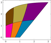
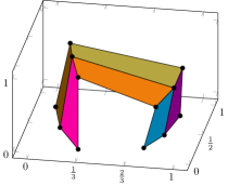
Figure 1: A polynomial membrane in $\mathbb{R}^{2}$ and a piecewise bilinear membrane in $\mathbb{R}^{3}$. The colors correspond to images of rectangles in a uniform partitioning of $[0,1]^{2}$. See Example 3.7 and Figure 3 for a more detailed description.

An implicitization problem.

Our strategy is to view the varieties (3) as solutions to an implicitization problem. To this end, we show that both classes of membranes admit a dictionary membrane (see [41]), i.e. a membrane which yields all other membranes in the class via linear transforms, up to certain terms that vanish under the signature map.

Our first candidate of a dictionary is the $mn$-dimensional moment membrane,

$$\mathsf{Mom}^{m,n}:[0,1]^{2} \to\mathbb{R}^{mn},(s,t)\mapsto(s,s^{2},\dots,s^{m})\otimes(t,t^{2},\dots,t^{n}),$$ (4)

where $\otimes$ is the Kronecker product. If $m=n=2$, then $\mathsf{Mom}^{2,2}(s,t)=(st,st^{2},s^{2}t,s^{2}t^{2})$ has the signature matrix

$$\sigma(\mathsf{Mom}^{2,2})=\begin{pmatrix}\frac{1}{4}&\frac{1}{3}&\frac{1}{3}&\frac{4}{9}\\[4.0pt] \frac{1}{6}&\frac{1}{4}&\frac{2}{9}&\frac{1}{3}\\[4.0pt] \frac{1}{6}&\frac{2}{9}&\frac{1}{4}&\frac{1}{3}\\[4.0pt] \frac{1}{9}&\frac{1}{6}&\frac{1}{6}&\frac{1}{4}\end{pmatrix}=\begin{pmatrix}\frac{1}{2}&\frac{2}{3}\\[4.0pt] \frac{1}{3}&\frac{1}{2}\end{pmatrix}\otimes\begin{pmatrix}\frac{1}{2}&\frac{2}{3}\\[4.0pt] \frac{1}{3}&\frac{1}{2}\end{pmatrix}$$ (5)

with a Kronecker factorization into path signatures (Corollary 3.6). Note that indeed every $d$-dimensional polynomial membrane $X$ with terms of multidegree $\geq(1,1)$ is of the form $X=A\,\mathsf{Mom}^{m,n}$. With equivariance of the signature (Lemma 2.6) we obtain the closed formula,

$$\sigma(X)=A\sigma(\mathsf{Mom}^{m,n})A^{\top},$$ (6)

as a matrix congruence. Hence, continuing with our example (5) and $d=2$, we have

$$X=A\,\mathsf{Mom}^{2,2}=\begin{pmatrix}a_{1,1}st+a_{1,2}st^{2}+a_{1,3}s^{2}t+a_{1,4}s^{2}t^{2}\\ a_{2,1}st+a_{2,2}st^{2}+a_{2,3}s^{2}t+a_{2,4}s^{2}t^{2}\end{pmatrix}$$ (7)

Thus, we obtain the first entry of our signature matrix from (5) and (6): It is the homogeneous polynomial

$$\sigma(X)_{1,1}=\frac{1}{4}a_{1,1}^{2} +\frac{1}{2}a_{1,1}a_{1,2}+\frac{1}{2}a_{1,1}a_{1,3}+\frac{5}{9}a_{1,1}a_{1,4}+\frac{1}{4}a_{1,2}^{2}$$

$$+\frac{4}{9}a_{1,2}a_{1,3}+\frac{1}{2}a_{1,2}a_{1,4}+\frac{1}{4}a_{1,3}^{2}+\frac{1}{2}a_{1,3}a_{1,4}+\frac{1}{4}a_{1,4}^{2}$$

of degree two. The remaining three polynomial entries of $\sigma(X)$ are provided in Example 3.7. We illustrate the polynomial membrane (7) for explicit $A$ in Figure 3.

The axis membrane.

Interpolation is a necessary step to fit discrete data into the framework of iterated integrals. Our second important dictionary, the axis membrane $\mathsf{Axis}^{m,n}$, is inspired by the dictionary for piecewise linear paths [2, 41] (see Definition 3.15). This $mn$-dimensional membrane allows us to interpolate arbitrary $d$-dimensional discrete data on an $m\times n$ grid via a piecewise bilinear membrane. For an illustration of such an interpolation see $Y$ from Figure 3. We provide novel closed-form expressions and computational complexity statements for its signatures (Theorem 3.19).

Main results.

Using our description via dictionaries, we obtain an analogue of [2, Theorem 3.3] for membranes:

Theorem (4.1).

For all $d,m$ and $n$,

$$\mathcal{P}^{\mathsf{pol}}_{d,m,n}=\mathcal{P}^{\mathsf{bil}}_{d,m,n}=:\mathcal{P}_{d,m,n}.$$

In fact, already the defining semi-algebraic sets agree.

These varieties are irreducible (Proposition 4.3) and we obtain a grid

$$\begin{matrix}\mathcal{P}_{d,1,1}&\subseteq&\mathcal{P}_{d,1,2}&\subseteq&\mathcal{P}_{d,1,3}&\subseteq&\dots&\subseteq&\mathcal{P}_{d,1,N}\\ \rotatebox[origin={c}]{270.0}{$\subseteq$}&&\rotatebox[origin={c}]{270.0}{$\subseteq$}&&\rotatebox[origin={c}]{270.0}{$\subseteq$}&&&&\rotatebox[origin={c}]{270.0}{$\subseteq$}\\ \mathcal{P}_{d,2,1}&\subseteq&\mathcal{P}_{d,2,2}&\subseteq&\mathcal{P}_{d,2,3}&\subseteq&\dots&\subseteq&\mathcal{P}_{d,2,N}\\ \rotatebox[origin={c}]{270.0}{$\subseteq$}&&\rotatebox[origin={c}]{270.0}{$\subseteq$}&&\rotatebox[origin={c}]{270.0}{$\subseteq$}&&&&\rotatebox[origin={c}]{270.0}{$\subseteq$}\\ \vdots&&\vdots&&\vdots&&\ddots&&\vdots\\ \rotatebox[origin={c}]{270.0}{$\subseteq$}&&\rotatebox[origin={c}]{270.0}{$\subseteq$}&&\rotatebox[origin={c}]{270.0}{$\subseteq$}&&&&\rotatebox[origin={c}]{270.0}{$\subseteq$}\\ \mathcal{P}_{d,M,1}&\subseteq&\mathcal{P}_{d,M,2}&\subseteq&\mathcal{P}_{d,M,3}&\subseteq&\dots&\subseteq&\mathcal{P}_{d,M,N}\end{matrix}$$ (8)

where we can choose $M,N\in\mathbb{N}$ such that

$$\mathcal{P}_{d,m,1}\subseteq\dots\subseteq\mathcal{P}_{d,m,N-1}\subseteq\mathcal{P}_{d,m,N}=\mathcal{P}_{d,m,N+1} =\dots\quad$$

$$\mathcal{P}_{d,1,n}\subseteq\dots\subseteq\mathcal{P}_{d,M-1,n}\subseteq\mathcal{P}_{d,M,n}=\mathcal{P}_{d,M+1,n} =\dots$$

for all $m,n\in\mathbb{N}$. As $\mathcal{P}_{d,1,m}=\mathcal{P}_{d,m,1}$ agrees with the path varieties studied in [2] (Lemma 4.5), it follows that $\mathcal{P}_{d,1,N}=\mathcal{P}_{d,M,1}$ is the universal path variety. However, in strong contrast to the path case, in general there are no algebraic relations in our two-parameter signature matrices (2) at all:

Theorem (4.7).

The limit variety $\mathcal{P}_{d,M,N}$ in (8) attains the full ambient dimension, i.e. $\mathcal{P}_{d,M,N}=\mathbb{C}^{d^{2}}$.

The varieties become more interesting if $m$ and $n$ are small compared to $d$. Employing the theory of orbits under congruence [45, 30] we were able to find explicit formulas for the dimensions of $\mathcal{P}_{d,m,n}$ whenever $mn\leq d$, generalizing [2, Theorem 3.4]. Note that there are $dmn\leq d^{2}$ parameters involved, so the dimension can be at most $dmn$.

Theorem (4.9).

For $mn\leq d$ the dimension of $\mathcal{P}_{d,m,n}$ is

• $dmn-\frac{1}{2}m^{2}n^{2}+m^{2}(n-1)+(m-1)n^{2}-\frac{7}{2}mn+4(m+n)-4$ for even $m,n$.

• $dmn-\frac{1}{2}m^{2}n^{2}+m^{2}(n-1)+(m-1)n^{2}-\frac{3}{2}mn+m+n$ for even $m$, odd $n$.

• $dmn-\frac{1}{2}m^{2}n^{2}+m^{2}(n-1)+(m-1)n^{2}-\frac{7}{2}mn+3(m+n)-2$ for odd $m,n$.

These results are complemented by some explicit computations using the open-source computer algebra systems Macaulay 2 [28, 19], and OSCAR [40, 13], see e.g. Examples 4.12 and 4.2, Remark 4.13 and Example 4.14.

Related work

The collection of iterated integrals of a path has been used as a tool for classification in various settings since Chen’s seminal 1954 work [8]. After pioneering work by Lyons and collaborators on the use of signatures as features for data streams in the early 2010s [29, 32], there has been a surge in the number of applications, which range from motion recognition [47], finance [4], deep learning [33, 34, 46, 35], oceanography [44], and lately data science for images [48, 31]. We refer the interested reader to the surveys [10, 38].

Since [2, 41, 24] established the initial connection between stochastic analysis and algebraic geometry, the signature has also been applied in various related fields, including the theory of tensor decompositions [3, 22, 25], clustering tasks [11, 39], tropical time series analysis [15, 16] and the geometry of paths [17, 1, 42].

Recently, the signature has been extended to two parameters, generalizing from paths to membranes: the mapping space signature [26] provides a principled two-parameter extension of Chen’s iterated integrals, based on its original use in topology, whereas the two-parameter sums signature [18] characterizes equivalence up to warping in two directions. These two approaches have recently been combined in [14] using mixed partial derivatives. Due to the lack of a two-parameter version of Chen’s identity in all the above references, recent works [9, 37, 36] use higher category theory to find an appropriate generalization of a group that is rich enough to represent the horizontal and vertical concatenation of membranes.

2 Iterated integrals

The iterated-integrals signature $\sigma=\sigma(X)$ of a $d$-dimensional path $X:[0,1]\to\mathbb{R}^{d}$ is an element of the tensor series algebra $T((\mathbb{R}^{d}))\cong\operatorname{Hom}(T(\mathbb{R}^{d}),\mathbb{R})$, defined by

$$\sigma:T(\mathbb{R}^{d}) \to\mathbb{R},$$

$$e_{i_{1}}\otimes\dots\otimes e_{i_{k}} \mapsto\int_{\Delta}\mathrm{d}X_{i_{1}}(t_{1})\dots\mathrm{d}X_{i_{k}}(t_{k}),$$ (9)

where $\Delta$ is the simplex $0<t_{1}<\dots<t_{k}<1$. It is common to write the tensor $e_{i_{1}}\otimes\dots\otimes e_{i_{k}}$ as a word $i_{1}\dots i_{k}$, identifying the tensor algebra with the free associative algebra over the letters 1 to d. However, the tensor algebra viewpoint allows us to consider the signature for paths (and later membranes) in any $\mathbb{R}$-vector space $V$, without choosing a basis, which will be useful in the following. Let us first recall some examples in the (classical, one-parameter) path setting.

Example 2.1.

1. For fixed $u\in\mathbb{R}^{d}$, the $k$-th signature tensor of the linear path $[0,1]\rightarrow\mathbb{R}^{d},t\mapsto ut$ is given by

   $$\sigma^{(k)}_{i_{1},\dots,i_{k}}=\frac{u_{i_{1}}\dots u_{i_{k}}}{k!}$$ (10)

   where $1\leq i_{1},\dots,i_{k}\leq d$.

2. Let $\mathsf{Axis}^{d}:[0,1]\to\mathbb{R}^{d}$ be the canonical axis path from [2, Example 2.1] or [41, eq. (8)] of order $d$, i.e., the unique piecewise linear path with $d$ segments whose graph interpolates the $d+1$ equidistant support points $(\frac{i}{d},\sum_{1\leq j\leq i}e_{j})$ with $0\leq i\leq d$. This path is illustrated in Figure 2 for $d=3$. For all $d$, its signature matrix is the upper triangular matrix

   $$\sigma^{(2)}_{i_{1},i_{2}}=\begin{cases}1&\text{if }i_{1}<i_{2}\\ \frac{1}{2}&\text{if }i_{1}=i_{2}\\ 0&\text{if }i_{1}>i_{2}.\end{cases}$$ (11)

3. We denote by $\mathsf{Mom}^{d}:[0,1]\to\mathbb{R}^{d},t\mapsto(t,\dots,t^{d})$ the moment path of degree $d$. We have the closed formula

   $$\sigma^{(k)}_{i_{1},i_{2},\dots,i_{k}}=\frac{i_{2}i_{3}\dots i_{k}}{(i_{1}+i_{2})(i_{1}+i_{2}+i_{3})\dots(i_{1}+\dots+i_{k})}$$ (12)

   for all $i_{1},\dots,i_{k}$ due to [2, Example 2.2].

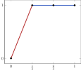
$\mathsf{graph}(\mathsf{Axis}^{3}_{1})$

$\mathsf{graph}(\mathsf{Axis}^{3}_{2})$

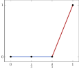
$\mathsf{graph}(\mathsf{Axis}^{3}_{3})$

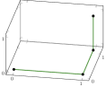
$\mathsf{Im}(\mathsf{Axis}^{3}$)

Figure 2: The $3$ graphs of the coordinate functions $\mathsf{Axis}^{3}_{i}$ with the non-constant part marked in red, and the entire image of the $3$-dimensional path $\mathsf{Axis}^{3}$ on the right. Compare also Figure 4 for the correspondending axis membrane.

In the following we recall the ‘nearest’ extension of the path signature (2) for multiple parameters and comment on its various modifications in Remark 2.3.

Definition 2.2.

Let $V$ be a finite dimensional vector space and $X:[0,1]^{p}\to V$ a Lipschitz continuous map. Let $\partial_{1\dots p}:=\frac{\partial^{p}}{\partial x_{1}\dots\partial x_{p}}$ be the linear partial differential operator. Then, since both the integral and $\partial_{1\dots p}$ are linear operators, the following linear form $\sigma=\sigma(X)\in T(V^{*})^{*}$ is well-defined:

$$\sigma:T(V^{*}) \to\mathbb{R},$$

$$\alpha_{1}\otimes\dots\otimes\alpha_{k} \mapsto\int_{\Delta^{p}}\partial_{1\dots p}(\alpha_{1}\circ X)(t_{11},\dots,t_{1p})\dots\partial_{1\dots p}(\alpha_{k}\circ X)(t_{k1},\dots,t_{kp})\,\mathrm{d}\mathbf{t}$$

where $\mathrm{d}\mathbf{t}=\mathrm{d}t_{11}\dots\mathrm{d}t_{1p}\dots\mathrm{d}t_{k1}\dots\mathrm{d}t_{kp}$ and $\Delta^{p}=\Delta\times\dots\times\Delta$ is the Cartesian product of $p$ simplices. We call $\sigma$ the iterated-integrals signature of $X$. The $k$-th level signature $\sigma^{(k)}(X)$ is the restriction of $\sigma(X)$ along $(V^{*})^{\otimes k}\to T(V^{*})$, in particular it is naturally an element of $V^{\otimes k}$.

Remark 2.3.

1. For the one-parameter framework $p=1$ in $d$-dimensional space $V=\mathbb{R}^{d}$ equipped with standard basis $e_{1},\dots,e_{d}$ we obtain the classical formulation (2) for paths. We refer the interested reader to the text books [23, 21].

2. When ‘replacing’ our square increments $\partial_{1\dots p}$ with Jacobian minors we obtain the $\mathsf{id}$-signature introduced in [26].

3. For membranes, that is $p=2$ parameters and standard basis $e_{1},\dots,e_{d}$ of $V=\mathbb{R}^{d}$, we obtain the $\mathsf{id}$-signature according to [14]. Its level $k$ component can be stored in the $d\times\dots\times d$ array,

   $$\sigma^{(k)}_{i_{1},\dots,i_{k}} :=\sigma(e_{i_{1}}\otimes\dots\otimes e_{i_{k}})$$

   $$=\int\limits_{\begin{subarray}{c}0<s_{1}<\dots<s_{k}<1\\ 0<t_{1}<\dots<t_{k}<1\end{subarray}}\partial_{12}X_{i_{1}}(s_{1},t_{1})\dots\partial_{12}X_{i_{k}}(s_{k},t_{k})\,\mathrm{d}s_{1}\mathrm{d}t_{1}\dots\mathrm{d}s_{k}\mathrm{d}t_{k}.$$

   In particular, for level $k=2$, we obtain our signature matrix $\sigma=\sigma^{(2)}$ from the introduction, (2).

4. When ‘replacing’ integrals by sums, and $\partial_{12}$ by its discrete counterpart, we obtain the two-parameter sums signature [18], evaluated at all diagonal matrix compositions. For this compare also [14, Example 4.16].

Remark 2.4.

It is clear from the definition that the signatures of any two Lipschitz continuous maps $X,Y:[0,1]^{p}\to V$ agree if $\partial_{1...p}(\alpha\circ(X-Y))=0$ for all $\alpha\in V^{*}$. For $p=1$ this is just the translation invariance of the signature, for membranes, i.e. $p=2$, this is invariance under adding terms only depending on one of the variables. In particular, if $X:[0,1]^{2}\to V$ is a membrane, we can always find a membrane $X_{\mathrm{red}}$ which vanishes on $[0,1]\times\{0\}\cup\{0\}\times[0,1]$ and has the same signature as $X$, by letting $X_{\mathrm{red}}(s,t):=X(s,t)-X(0,t)-X(s,0)+X(0,0)$. See also Lemma 3.18 and Figure 4 for an illustration of piecewise bilinear membranes.

We provide some first examples for membranes ($p=2$).

Example 2.5.

1. For fixed $u\in\mathbb{R}^{d}$, the $k$-th signature tensor of the $d$-dimensional bilinear membrane $[0,1]^{2}\rightarrow\mathbb{R}^{d},(s,t)\mapsto ust$ is given by

   $$\sigma^{(k)}_{i_{1},\dots,i_{k}}=\frac{u_{i_{1}}\dots u_{i_{k}}}{(k!)^{2}}$$ (13)

   where $1\leq i_{1},\dots,i_{k}\leq d$. This formula follows from Corollary 3.5 or can be verified by an immediate computation.

2. We recall the $2$-dimensional polynomial membrane $X=A\,\mathsf{Mom}^{2,2}$ from the introduction, (7). With integration over the differentials of the two-parameter moment coordinates,

   $$\int_{0}^{1}\int_{0}^{1}\,\mathrm{d}s\mathrm{d}t=\int_{0}^{1}\int_{0}^{1}2t\,\mathrm{d}s\mathrm{d}t=\int_{0}^{1}\int_{0}^{1}2s\,\mathrm{d}s\mathrm{d}t=\int_{0}^{1}\int_{0}^{1}4st\,\mathrm{d}s\mathrm{d}t=1,$$

   we obtain, together with linearity, the level $1$ signature,

   $$\sigma^{(1)}(X)=\begin{pmatrix}a_{1,1}+a_{1,2}+a_{1,3}+a_{1,4}\\ a_{2,1}+a_{2,2}+a_{2,3}+a_{2,4}\end{pmatrix}\in\mathbb{R}^{2}.$$

   In Example 3.7 and 3.11 we provide closed formulas for its level $2$ and $3$ signature tensors, respectively.

As in the previous example, we can use linearity of the integral to compute level $k$ signatures of transformed functions by corresponding actions on tensors.

Lemma 2.6 (Equivariance).

Let $V,W$ be finite dimensional $\mathbb{R}$-vector spaces, and $X:[0,1]^{p}\to V$ be a Lipschitz continuous map. If $A:V\to W$ is linear, then $\sigma(AX)=\sigma(X)\circ T(A^{*})$.

Proof.

This follows immediately from the definition, since for $w=w_{1}\otimes\dots\otimes w_{k}$ (where $w_{i}\in W^{*}$) we have $w_{i}\circ(A\circ X)=(w_{i}\circ A)\circ X=A^{*}(w_{i})\circ X$. ∎

In particular, Lemma 2.6 implies that $\sigma^{(k)}(AX)=A^{\otimes k}(\sigma^{(k)}(X))$ for all $k$. If $V=\mathbb{R}^{d}$ we can write this in the Tucker format $\sigma^{(k)}(AX)=[\![\sigma^{(k)}(X);A,\dots,A]\!]$. Explicitly, if $k=2$ we have

$$\sigma^{(k)}(AX)=A\sigma^{(k)}(X)A^{\top},$$

as was already mentioned in the introduction (6). The equivariance of signatures is a key property used in [41], allowing the computation of signature tensors for various families of paths from a small collection of dictionaries, also called core tensors. In the following section we introduce such dictionaries for membranes.

3 Product membranes

Some membranes arise from combining paths: given a path $[0,1]\to V$ and another path $[0,1]\to W$ we can consider the Cartesian product $[0,1]^{2}\to V\times W$. Composing this with any suitable function $\phi:V\times W\to Z$ into another vector space $Z$ yields a membrane. The first goal of this section is to show that if $\phi$ is bilinear, then we can express the signature of the resulting membrane in terms of the signatures of the defining paths. This is particularly important for us, as we will see that both polynomial and piecewise bilinear membranes can be obtained in this way. Recalling equivariance of the signature (Lemma 2.6) and that any bilinear map $V\times W\to Z$ factors over a linear map $V\otimes W\to Z$, it suffices to understand the signature of the following type of membrane:

Definition 3.1.

Let $V$ and $W$ be finite dimensional vector spaces. The product membrane of two paths $X:[0,1]\to V$ and $Y:[0,1]\to W$ is the membrane in the tensor product $V\otimes W$ induced by the Cartesian product:

$$X\boxtimes Y:[0,1]^{2}\to V\times W\to V\otimes W.$$

In other words, $X\boxtimes Y(s,t):=X(s)\otimes Y(t)$ for all $(s,t)\in[0,1]^{2}$.

Example 3.2.

1. Consider the path $X$ mapping $s\mapsto(s,s^{2})$ and the path $Y$ mapping $t\mapsto(e^{t},\log(1+t))$. Writing elements of $\mathbb{R}^{2}\otimes\mathbb{R}^{2}$ as matrices, the product membrane $X\boxtimes Y$ is given by

   $$(s,t)\mapsto\begin{pmatrix}se^{t}&s\log(1+t)\\ s^{2}e^{t}&s^{2}\log(1+t)\end{pmatrix}\in\mathbb{R}^{2\times 2}.$$

2. The moment membrane of multidegree $(m,n)$ in the introduction (4) is the product

   $$\mathsf{Mom}^{m,n}=\mathsf{Mom}^{m}\boxtimes\mathsf{Mom}^{n}:[0,1]^{2} \to\mathbb{R}^{m}\otimes\mathbb{R}^{n},$$ (14)

   where the moment path $\mathsf{Mom}^{m}$ is according to Example 2.1. Note that we sometimes omit the last vectorization, i.e., we identity $\mathbb{R}^{m\times n}$ with $\mathbb{R}^{mn}$ whenever the context allows this. For this compare also Corollary 3.6. Note that every $d$-dimensional polynomial membrane $X$ with multidegree $(m,n)$ without terms of degree $\leq(1,1)$ is of the form $X=A\circ\mathsf{Mom}^{m,n}$, where $A$ is a linear map, e.g. our running Example 2.5 with $m=n=d=2$.

3.1 Factorizations into path signatures

We state our main result of this section, Proposition 3.3, showing that the signature is multiplicative with respect to products of paths (Definition 3.1). In Corollary 3.6, we rephrase this for the matrix case $k=2$, with explicit vectorizations and the use of the Kronecker matrix product. We illustrate these results in Examples 3.11 and 3.7, respectively.

Proposition 3.3.

Let $X\boxtimes Y:[0,1]^{2}\to V\otimes W$ be a product membrane. Then, as linear maps,

$$\sigma(X\boxtimes Y)=\sigma(X)\otimes\sigma(Y)$$

in the following sense: the map $\sigma(X\boxtimes Y)$ factors as

$$T((V\otimes W)^{*})\stackrel{{\scriptstyle\sim}}{{\smash{\longleftarrow}\rule{0.0pt}{1.72218pt}}}T(V^{*}\otimes W^{*})\to T(V^{*})\otimes T(W^{*})\to\mathbb{R},$$

where the second map is induced by the universal property of the tensor algebra, and the last map is given by $\sigma(X)\otimes\sigma(Y)$. More explicitly, for all $k\geq 1$, $\alpha_{i}\in V^{*}$, $\beta_{i}\in W^{*}$ we have

$$\left<\sigma(X\boxtimes Y),(\alpha_{1}\otimes\beta_{1})\otimes\dots\otimes(\alpha_{k}\otimes\beta_{k})\right> =$$

$$\left<\sigma(X),\alpha_{1}\otimes\dots\otimes\alpha_{k}\right> \cdot\left<\sigma(Y),\beta_{1}\otimes\dots\otimes\beta_{k}\right>$$

Caveat 3.4.

Note that the tensor product of linear forms $\sigma(X):T(V^{*})\to\mathbb{R}$, $\sigma(Y):T(V^{*})\to\mathbb{R}$ is not the tensor product in the tensor series space $T(V^{*})$; the formula above should not be confused with Chen’s formula for the signature of a concatenation of paths.

Before proving Proposition 3.3, we provide examples and discuss several implications. As a first application, we compute the signature of product membranes where one path is $1$-dimensional, explaining for instance our example (13) using path signatures.

Corollary 3.5.

Let $X:[0,1]\to\mathbb{R}$ be a $1$-dimensional path, and $Y:[0,1]\to W$ be arbitrary. Then $\sigma(X\boxtimes Y)$ is a map $T(\mathbb{R}\otimes W^{*})\to\mathbb{R}$, so we can view it as a map $T(W^{*})\to\mathbb{R}$. Then it sends a simple tensor $w=w_{1}\otimes\dots\otimes w_{\ell}$ to

$$\sigma(X)(e_{1}^{\otimes\ell})\cdot\sigma(Y)(w)=\frac{(X(1)-X(0))^{\ell}}{\ell!}\cdot\sigma(Y)(w).$$

In particular, $\sigma^{(k)}(X\boxtimes Y)=\frac{1}{k!}(X(1)-X(0))^{k}\cdot\sigma^{(k)}(Y)$, so $\sigma^{(k)}(X\boxtimes Y)$ and $\sigma^{(k)}(Y)$ differ only by some scalar for any $k$.

Proof.

Unravel the factorization of $\sigma(X\boxtimes Y)$ in Proposition 3.3. ∎

If $X:[0,1]^{2}\to V\otimes W$ is a product membrane, it can be convenient to use a vectorization $\nu:V\otimes W\cong\mathbb{R}^{\dim V}$, for example to obtain an actual signature matrix. Using Lemma 2.6, we see that $\sigma(\nu X)$ then factors as

$$T(\mathbb{R}^{d})\to T((V\otimes W)^{*})\to T(V^{*})\otimes T(W^{*})\to\mathbb{R}$$

where the first map is $T(\nu^{*})$.

As a special case, we obtain compatibility of the signature with the Kronecker product of paths:

Corollary 3.6.

Let $X:[0,1]\to\mathbb{R}^{m}$ and $Y:[0,1]\to\mathbb{R}^{n}$ be two paths and let $\mathsf{kron}(X,Y):[0,1]^{2}\to\mathbb{R}^{mn}$ denote the membrane that maps $(s,t)$ to the Kronecker product of the column vectors $X(s)$ and $Y(t)$. Then

$$\sigma^{(2)}(\mathsf{kron}(X,Y)) =\sigma^{(2)}(X)\otimes\sigma^{(2)}(Y)$$

where $\otimes$ denotes the Kronecker product of matrices.

Example 3.7.

We return to our running Example 2.5 with $X=A\,\mathsf{Mom}^{2,2}$ and matrix $A=(a_{i,j})_{1\leq i\leq 2,1\leq j\leq 4}$. With Corollary 3.6 and (12) we get the core matrix of the moment membrane,

$$C^{(2)}:=\sigma^{(2)}(\mathsf{vec}\circ\mathsf{Mom}^{2,2})=\sigma^{(2)}(\mathsf{Mom}^{2})\otimes\sigma^{(2)}(\mathsf{Mom}^{2})=\begin{pmatrix}\frac{1}{2}&\frac{2}{3}\\[4.0pt] \frac{1}{3}&\frac{1}{2}\end{pmatrix}\otimes\begin{pmatrix}\frac{1}{2}&\frac{2}{3}\\[4.0pt] \frac{1}{3}&\frac{1}{2}\end{pmatrix}$$

as it is presented in the introduction, (5). With $S^{(2)}:=\sigma^{(2)}(X)=AC^{(2)}A^{\top}$ we provide the three missing homogeneous entries,

$$S^{(2)}_{2,1} =\frac{1}{4}a_{1,1}a_{2,1}+\frac{1}{6}a_{1,1}a_{2,2}+\frac{1}{6}a_{1,1}a_{2,3}+\frac{1}{9}a_{1,1}a_{2,4}+\frac{1}{3}a_{2,1}a_{1,2}+\frac{1}{3}a_{2,1}a_{1,3}$$

$$\quad+\frac{4}{9}a_{2,1}a_{1,4}+\frac{1}{4}a_{1,2}a_{2,2}+\frac{2}{9}a_{1,2}a_{2,3}+\frac{1}{6}a_{1,2}a_{2,4}+\frac{2}{9}a_{2,2}a_{1,3}+\frac{1}{3}a_{2,2}a_{1,4}$$

$$\quad+\frac{1}{4}a_{1,3}a_{2,3}+\frac{1}{6}a_{1,3}a_{2,4}+\frac{1}{3}a_{2,3}a_{1,4}+\frac{1}{4}a_{1,4}a_{2,4}$$

$$S^{(2)}_{1,2} =\frac{1}{4}a_{1,1}a_{2,1}+\frac{1}{3}a_{1,1}a_{2,2}+\frac{1}{3}a_{1,1}a_{2,3}+\frac{4}{9}a_{1,1}a_{2,4}+\frac{1}{6}a_{2,1}a_{1,2}+\frac{1}{6}a_{2,1}a_{1,3}$$

$$\quad+\frac{1}{9}a_{2,1}a_{1,4}+\frac{1}{4}a_{1,2}a_{2,2}+\frac{2}{9}a_{1,2}a_{2,3}+\frac{1}{3}a_{1,2}a_{2,4}+\frac{2}{9}a_{2,2}a_{1,3}+\frac{1}{6}a_{2,2}a_{1,4}$$

$$\quad+\frac{1}{4}a_{1,3}a_{2,3}+\frac{1}{3}a_{1,3}a_{2,4}+\frac{1}{6}a_{2,3}a_{1,4}+\frac{1}{4}a_{1,4}a_{2,4}$$

and

$$S^{(2)}_{2,2} =\frac{1}{4}a_{2,1}^{2}+\frac{1}{2}a_{2,1}a_{2,2}+\frac{1}{2}a_{2,1}a_{2,3}+\frac{5}{9}a_{2,1}a_{2,4}+\frac{1}{4}a_{2,2}^{2}+\frac{4}{9}a_{2,2}a_{2,3}+\frac{1}{2}a_{2,2}a_{2,4}$$

$$\quad+\frac{1}{4}a_{2,3}^{2}+\frac{1}{2}a_{2,3}a_{2,4}+\frac{1}{4}a_{2,4}^{2}$$

using equivariance, Lemma 2.6. The polynomial $S_{1,1}^{(2)}$ is already provided in the introduction.

We illustrate the membrane $X$ in the first row of Figure 3, for $A=\begin{pmatrix}1&-1&1&1\\ 1&1&0&-1\end{pmatrix}$. In particular, we provide the graphs of the coordinate functions $\mathsf{graph}(X_{1})$ and $\mathsf{graph}(X_{2})$, and a plot of the image $\mathsf{Im}(X)$ in $\mathbb{R}^{2}$. Here, the colors correspond to the image of rectangles in a uniform partition of $[0,1]^{2}$, e.g. $X([0,\frac{1}{3}]\times[0,\frac{1}{2}])$ in pink, $X([\frac{1}{3},\frac{2}{3}]\times[0,\frac{1}{2}])$ in orange, or $X([\frac{2}{3},1]\times[\frac{1}{2},1])$ in violet. Note that $X$ maps three sides of the square $[0,1]^{2}$ to the origin. The right-most picture shows an ”untangled” version of the membrane $X$ which has the same signature, cf. Remark 2.4.

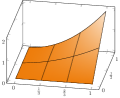
$\mathsf{graph}(X_{1})$

$\mathsf{graph}(X_{2})$

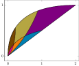
$\mathsf{Im}(X)$

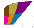
$\mathsf{Im}(X+\begin{pmatrix}s\\ 2t\end{pmatrix})$

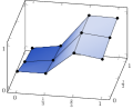
$\mathsf{graph}(Y_{1})$

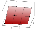
$\mathsf{graph}(Y_{2})$

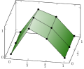
$\mathsf{graph}(Y_{3})$

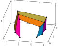
$\mathsf{Im}(Y)$

Figure 3: Plots of the polynomial membrane $X$ in $\mathbb{R}^{2}$ from Example 3.7 and a piecewise bilinear membrane $Y$ interpolating $12$ points in $\mathbb{R}^{3}$, represented by black dots. Let $X_{1},X_{2},Y_{1},Y_{2}$ and $Y_{3}$ denote the coordinate functions of $X$ and $Y$, respectively.

Proof of Corollary 3.6.

Choosing the vectorization $\nu:\mathbb{R}^{m}\otimes\mathbb{R}^{n}\to\mathbb{R}^{mn},e_{i}\otimes e_{j}\mapsto e_{n(i-1)+j}$, we see that $\mathsf{kron}=\nu\circ X\boxtimes Y$. Then we have

$$\left<\sigma(\nu(X\boxtimes Y)),e_{i}\otimes e_{j}\right>=\left<\sigma(X\boxtimes Y),\nu^{*}(e_{i})\otimes\nu^{*}(e_{j})\right>$$

$$=\left<\sigma(X\boxtimes Y),(e_{i_{1}}\otimes e_{i_{2}})\otimes(e_{j_{1}}\otimes e_{j_{2}})\right>=\left<\sigma(X),e_{i_{1}}\otimes e_{j_{1}}\right>\cdot\left<\sigma(Y),e_{i_{2}}\otimes e_{j_{2}}\right>$$

where $i_{1}=\lceil\frac{i}{n}\rceil$, $j_{1}=\lceil\frac{j}{n}\rceil$, $i_{2}=(i-1\text{ mod }n)+1$, $j_{2}=(j-1\text{ mod }n)+1$. In terms of signature matrices, this amounts to the identity

$$\sigma^{(2)}(\nu(X\boxtimes Y))=\sigma^{(2)}(X)\otimes\sigma^{(2)}(Y).$$

∎

As another consequence of Proposition 3.3 and equivariance we obtain the formula from [14, Example 4.2] for the Hadamard product of two paths:

Corollary 3.8.

If $V=W=\mathbb{R}^{d}$ then

$$\sigma(\mu(X\boxtimes Y))=\sigma(X)\cdot\sigma(Y)$$ (15)

as morphisms $T(\mathbb{R}^{d})\to\mathbb{R}$, and where $\mu:\mathbb{R}^{d}\otimes\mathbb{R}^{d}\to\mathbb{R}^{d}$ is the componentwise multiplication map.

Proof.

The dual map $\mu^{*}$ sends $e_{i}$ to $e_{i}\otimes e_{i}$. ∎

We close this section with our omitted proof, followed by an example for higher tensor levels, and an implication for the computational complexity of the signature of a polynomial membrane.

Proof of Proposition 3.3.

The isomorphism $T(V^{*}\otimes W^{*})\to T((V\otimes W)^{*})$ displayed in the statement is induced by the map that sends $\alpha\otimes\beta$ to the form $\alpha\cdot\beta$ on $V\otimes W$. Now, by definition, $\sigma(X)$ maps a simple tensor $\alpha_{1}\cdot\beta_{1}\otimes\dots\otimes\alpha_{k}\cdot\beta_{k}$ to

$$\int_{\Delta}\int_{\Delta}\prod_{i}\partial_{12}z_{i}(s_{i},t_{i})\,\mathrm{d}s_{1}\dots\mathrm{d}s_{k}\mathrm{d}t_{1}\dots\mathrm{d}t_{k}$$

where $z_{i}(s,t):=(\alpha_{i}\circ X)(s)\cdot(\beta_{i}\circ Y)(t)$. Here we reordered the differential forms which is allowed because we are integrating over the product simplex $\Delta^{2}$. In particular, we have $(\partial_{12}z_{i})(s,t)=\partial(\alpha_{i}\circ X)(s)\cdot\partial(\beta_{i}\circ Y)(t)$. By definition,

$$\langle\sigma(X^{(1)}),\alpha_{1}\otimes\dots\otimes\alpha_{k}\rangle=\int_{\Delta}\prod_{i}\partial(\alpha_{i}\circ X)(s_{i})\,\mathrm{d}s_{1}\dots\mathrm{d}s_{k}$$

and similarly for $Y$; thus reordering the integral reveals the claimed equality. ∎

Remark 3.9.

Proposition 3.3 and its proof immediately generalize to higher $p$-parameter patches $[0,1]^{p}\rightarrow\mathbb{R}^{d}$.

In order to provide an explicit computation for higher tensor levels $k\geq 3$, we introduce some further notation.

Remark and Notation 3.10.

If $X:[0,1]\to\mathbb{R}^{m}$ and $Y:[0,1]\to\mathbb{R}^{n}$ are two paths, then by Proposition 3.3 the signature of $X\boxtimes Y$ is a linear form on $T((\mathbb{R}^{m}\otimes\mathbb{R}^{n})^{*})$ which can be identified with the free associative algebra $\mathbb{R}\langle(i,j)\rangle$ over tuples of letters $i\in[m]$ and $j\in[n]$. Thus, in the following we also write $(i_{1},j_{1})\dots(i_{k},j_{k})$ for the tensor $(e_{i_{1}}\otimes e_{j_{1}})^{*}\otimes\dots\otimes(e_{i_{k}}\otimes e_{j_{k}})^{*}$.

Example 3.11.

With Proposition 3.3, our identification in 3.10, and the closed formula for signatures of polynomial paths in Example 2.1, we obtain a closed formula for the level $k$ tensor of the moment membrane $\mathsf{Mom}^{m,n}$ from (14),

$$\langle\sigma(\mathsf{Mom}^{m,n}),(i_{1},j_{1})\dots(i_{k},j_{k})\rangle=\frac{i_{2}\dots i_{k}}{(i_{1}+i_{2})\dots(i_{1}+\dots+i_{k})}\frac{j_{2}\dots j_{k}}{(j_{1}+j_{2})\dots(j_{1}+\dots+j_{k})}$$

where $i_{1},\dots,i_{k}\in[m]$ and $j_{1},\dots,j_{k}\in[n]$. For instance for the $2$-dimensional polynomial membrane from our running example Example 2.5, we obtain the level $k=3$ core tensor

$$C^{(3)}:=\scriptsize\left(\begin{array}[]{cccc|cccc|cccc|cccc}\frac{1}{36}&\frac{1}{36}&\frac{1}{36}&\frac{1}{36}&\frac{1}{24}&\frac{2}{45}&\frac{1}{24}&\frac{2}{45}&\frac{1}{24}&\frac{1}{24}&\frac{2}{45}&\frac{2}{45}&\frac{1}{16}&\frac{1}{15}&\frac{1}{15}&\frac{16}{225}\\[4.0pt] \frac{1}{72}&\frac{1}{60}&\frac{1}{72}&\frac{1}{60}&\frac{1}{45}&\frac{1}{36}&\frac{1}{45}&\frac{1}{36}&\frac{1}{48}&\frac{1}{40}&\frac{1}{45}&\frac{2}{75}&\frac{1}{30}&\frac{1}{24}&\frac{8}{225}&\frac{2}{45}\\[4.0pt] \frac{1}{72}&\frac{1}{72}&\frac{1}{60}&\frac{1}{60}&\frac{1}{48}&\frac{1}{45}&\frac{1}{40}&\frac{2}{75}&\frac{1}{45}&\frac{1}{45}&\frac{1}{36}&\frac{1}{36}&\frac{1}{30}&\frac{8}{225}&\frac{1}{24}&\frac{2}{45}\\[4.0pt] \frac{1}{144}&\frac{1}{120}&\frac{1}{120}&\frac{1}{100}&\frac{1}{90}&\frac{1}{72}&\frac{1}{75}&\frac{1}{60}&\frac{1}{90}&\frac{1}{75}&\frac{1}{72}&\frac{1}{60}&\frac{4}{225}&\frac{1}{45}&\frac{1}{45}&\frac{1}{36}\end{array}\right)$$

of shape $4\times 4\times 4$, and with equivariance (Lemma 2.6), the level $k=3$ signature tensor $\sigma^{(3)}(X)=[\![C^{(3)};A,A,A]\!]$ of shape $2\times 2\times 2$. We provide its first homogeneous entry,

$${\sigma^{(3)}(X)}_{1,1,1} =\frac{1}{36}a_{1,1}^{3}+\frac{1}{12}a_{1,1}^{2}a_{1,2}+\frac{1}{12}a_{1,1}^{2}a_{1,3}+\frac{7}{72}a_{1,1}^{2}a_{1,4}+\frac{1}{12}a_{1,1}a_{1,2}^{2}$$

$$\quad+\frac{11}{72}a_{1,1}a_{1,2}a_{1,3}+\frac{13}{72}a_{1,1}a_{1,2}a_{1,4}+\frac{1}{12}a_{1,1}a_{1,3}^{2}+\frac{13}{72}a_{1,1}a_{1,3}a_{1,4}$$

$$\quad+\frac{89}{900}a_{1,1}a_{1,4}^{2}+\frac{1}{36}a_{1,2}^{3}+\frac{5}{72}a_{1,2}^{2}a_{1,3}+\frac{1}{12}a_{1,2}^{2}a_{1,4}$$

$$\quad+\frac{5}{72}a_{1,2}a_{1,3}^{2}+\frac{34}{225}a_{1,2}a_{1,3}a_{1,4}+\frac{1}{12}a_{1,2}a_{1,4}^{2}+\frac{1}{36}a_{1,3}^{3}$$

$$\quad+\frac{1}{12}a_{1,3}^{2}a_{1,4}+\frac{1}{12}a_{1,3}a_{1,4}^{2}+\frac{1}{36}a_{1,4}^{3}.$$

The other (polynomial) entries of $\sigma^{(3)}(X)$ are similar and are therefore omitted here.

Inspired by [18, Theorem 4.5], we obtain the following computational implication.

Corollary 3.12.

For every $d$-dimensional polynomial membrane $X$ of multi-degree $(m,n)$ we can compute $\sigma^{(k)}(X)$ in $\mathcal{O}(m^{k}n^{k}+kd^{k+1}mn)$ elementary operations.

Proof.

We use the closed formula in Example 3.11 and $\mathsf{vec}^{\otimes k}$ to obtain the core tensor $C^{(k)}$ in $\mathcal{O}(m^{k}n^{k})$. The remaining follows with equivariance. ∎

Remark 3.13.

We can generalize Corollary 3.12 for any class of membranes which are induced via linear transforms of product membranes, e.g., piecewise bilinear membranes from the next section. Note that for the latter we can improve the analogous computational complexity bound by Theorem 3.19.

3.2 Dictionaries for bilinear interpolation

Definition 3.14.

A piecewise bilinear membrane is a membrane $X$ such that there are some $m,n\in\mathbb{N}$ with the property that $X$ is biaffine on all squares $[\frac{i-1}{m},\frac{i}{m}]\times[\frac{j-1}{n},\frac{j}{n}]$ with $i\in[m]$ and $j\in[n]$. We say that $X$ has order $(m,n)$.

Our interest in this class of membranes is threefold: from the path case, examined in [2], we expect a certain relation of this class of membranes to the polynomial membranes in terms of their signatures, e.g. Theorem 4.1. We also know that the recovery problem is solvable for piecewise linear paths of low order from [41, Corollary 6.3], and we would like to obtain a similar result for membranes (5.4). Finally, they form a rather natural class that can be used for the interpolation of discrete data to fit into the frame of iterated integrals, e.g. image data used in [48].

Bilinear interpolation of $d$-dimensional discrete data, arranged on an $(m+1)\times(n+1)$ grid, is a well-known procedure, e.g. in image processing [6, Chapter 3.7.2] or in the field of finite elements [49, Chapters 5.1.3.2 and 6.2.2.1], [20, Chapter 1.3.2]. The approach involves considering the four (unique) nodal bilinear basis functions on the reference rectangle, where each function is $1$ at one corner and $0$ at all others. The nodal basis on any arbitrary rectangle is then obtained through a linear transformation to the reference rectangle. Bilinear interpolation is simply the linear combination of the nodal basis functions, where the coefficients correspond exactly to the function values of the function being interpolated at the four grid points.

As in the polynomial case (14) we provide a product dictionary for piecewise bilinear membranes, so that its signature can be computed via Proposition 3.3. For this, we have already recalled in Example 2.1 the canonical axis path $\mathsf{Axis}^{m}$, which is illustrated in Figure 2 for $m=3$. The resulting axis membrane takes the role of the above mentioned bases for interpolation. It is illustrated for order $(3,2)$ in Figure 4.

Definition 3.15.

The (canonical) axis membrane of order $(m,n)$ is the product

$$\mathsf{Axis}^{m,n}:=\mathsf{Axis}^{m}\boxtimes\mathsf{Axis}^{n}:[0,1]^{2} \to\mathbb{R}^{m}\otimes\mathbb{R}^{n},$$ (16)

according to Definition 3.1.

Any piecewise linear path with $m$ segments starting at the origin can be realized through a suitable linear transformation of $\mathsf{Axis}^{m}$. We want to show that the analogue is true for membranes, i.e., (16) is a suitable dictionary for all piecewise bilinear membranes of order $(m,n)$ which map the coordinate axes $[0,1]\times 0\cup 0\times[0,1]$ to the origin. Let us first describe the axis membrane a bit more explicitly.

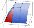
$\mathsf{Axis}^{3,2}_{1,1}$

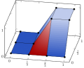
$\mathsf{Axis}^{3,2}_{2,1}$

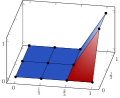
$\mathsf{Axis}^{3,2}_{3,1}$

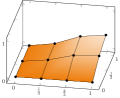
$A\circ\mathsf{Axis}_{3,2}$

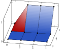
$\mathsf{Axis}^{3,2}_{1,2}$

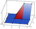
$\mathsf{Axis}^{3,2}_{2,2}$

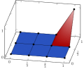
$\mathsf{Axis}^{3,2}_{3,2}$

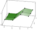
$R$

Figure 4: On the left we have the $6$ graphs of the coordinate functions from the axis membrane $\mathsf{Axis}^{3,2}$, with the non-linear rectangle marked in red, and the equidistant support points from (3.2) in black. On the right we illustrate the decomposition of the $1$-dimensional piecewise bilinear membrane $Y_{1}$ from Figure 3 into the linear transform of the axis membrane $A\circ\mathsf{Axis}^{3,2}$ and the linear part $R$ according to Lemma 3.18.

Lemma 3.16.

We consider the codomain from the axis membrane (16) as a space of matrices, that is $\mathsf{Axis}^{m,n}:[0,1]^{2}\rightarrow\mathbb{R}^{m\times n}$. Then each of its coordinate functions is piecewise bilinear,

$$\mathsf{Axis}^{m,n}_{i,j}(s,t):=\scriptsize\begin{cases}0&s\leq\frac{i-1}{m}\text{ or }t\leq\frac{j-1}{n}\\ mnst+m(1-j)s+n(1-i)t+(i-1)(j-1)&\frac{i-1}{m}<s\leq\frac{i}{m}\text{ and }\frac{j-1}{n}<t\leq\frac{j}{n}\\ nt+1-j&\frac{i}{m}<s\text{ and }\frac{j-1}{n}<t\leq\frac{j}{n}\\ ms+1-i&\frac{i-1}{m}<s\leq\frac{i}{m}\text{ and }\frac{j}{n}<t\\ 1&\frac{i}{m}<s\text{ and }\frac{j}{n}<t,\end{cases}$$

where $i\in[m]$, $j\in[n]$ and $s,t\in[0,1]$.

Proof.

Despite this being well-known we provide a bilinear interpolation in each of the $mn$ dimensions, i.e., we search for coefficients $c\in\mathbb{R}^{4}$ such that

$$\psi_{i,j}:\left[\frac{i-1}{m},\frac{i}{m}\right]\times\left[\frac{j-1}{n},\frac{j}{n}\right] \rightarrow\mathbb{R},(s,t)\mapsto c_{1}st+c_{2}s+c_{3}t+c_{4}$$

satisfies the system

$$\psi_{i,j}\left(\frac{i-1}{m},\frac{j-1}{n}\right) =0,\quad\psi_{i,j}\left(\frac{i}{m},\frac{j-1}{n}\right)=0,$$

$$\psi_{i,j}\left(\frac{i-1}{m},\frac{j}{n}\right) =0,\quad\psi_{i,j}\left(\frac{i}{m},\frac{j}{n}\right)=1.$$ (17)

By solving (3.2) in $c$ we obtain $c=\left(mn,m(1-j),n(1-i),(i-1)(j-1)\right)$ and hence $\psi=\mathsf{Axis}^{m,n}$ when restricted on the square $\left[\frac{i-1}{m},\frac{i}{m}\right]\times\left[\frac{j-1}{n},\frac{j}{n}\right]$. The claim follows with a similar (linear) system for the remaining squares. ∎

With the product structure in (16) we can use Proposition 3.3 to compute its core signature tensor with the help of the core signature tensors of axis paths.

Example 3.17.

From [2, Example 2.1] we know that $\sigma(\mathsf{Axis}^{m})_{i_{1},\dots,i_{k}}$ is zero unless $i_{1}\leq\dots\leq i_{k}$, and $\frac{1}{k!}$ times the number of distinct permutations of the string $i_{1}\dots i_{k}$ otherwise. Explicitly, with (11) the signature matrix is

$$\langle\sigma(\mathsf{Axis}^{m,n}),(i_{1},j_{1})(i_{2},j_{2})\rangle:=\begin{cases}1&i_{1}<i_{2}\text{ and }j_{1}<j_{2}\\ \frac{1}{2}&i_{1}=i_{2}\text{ and }j_{1}<j_{2}\\ \frac{1}{2}&i_{1}<i_{2}\text{ and }j_{1}=j_{2}\\ \frac{1}{4}&i_{1}=i_{2}\text{ and }j_{1}=j_{2}\\ 0&\text{otherwise.}\end{cases}$$

Recall from Remark 2.4 that we can always restrict our computations to membranes which are $0$ on the coordinate axes.

Lemma 3.18.

Every piecewise bilinear membrane $X$ has a (unique) decomposition

$$X=A\circ\mathsf{Axis}^{m,n}+R$$ (18)

where $\mathsf{Axis}^{m,n}$ is according to (16), $A$ is a linear transform, and $R$ is a piecewise linear (not bilinear) membrane in the two arguments $s$ and $t$. Then,

$$\sigma(X)=\sigma(A\circ\mathsf{Axis}^{m,n}).$$

Proof.

Clearly, $\{\mathsf{Axis}^{m,n}_{i,j}\mid i,j\}$ is an $\mathbb{R}$-basis of the space of $1$-dimensional piecewise bilinear membranes which are $0$ on $[0,1]\times 0\cup 0\times[0,1]$. We can extend this basis via $m+n-1$ functions which are piecewise linear in $s$ and constant in $t$, or vice versa. Applying a basis decomposition in each dimension, we obtain $A$ and $R$ in (18) for all $d$ and conclude by Remark 2.4. ∎

The decomposition is illustrated in Figure 4. See also [18, Lemma 2.22] for a similar result applied on discrete data, using two-parameter sums signatures.

Theorem 3.19.

Let $X$ be a piecewise bilinear membrane in $\mathbb{R}^{d}$ of order $(m,n)$ and $w\in T(\mathbb{R}^{d})$ a word of length $k$. Then we can compute $\langle\sigma(X),w\rangle$ in $\mathcal{O}(k^{2}mn^{k})$.

Proof.

With Lemma 3.18 we assume that $X$ is $0$ on $\{0\}\times[0,1]\cup[0,1]\times\{0\}$. Let $\Lambda$ denote the piecewise linear path in $\mathbb{R}^{n}$ of order $n$ with control points $(0,e_{1},\dots,e_{n})$. Then we can write

$$X(s,t)=\sum_{i=0}^{n}X(s,\frac{i}{n})\Lambda_{i}(t)$$

Indeed, the right hand side is clearly piecewise bilinear of order $(m,n)$ and agrees with $X$ on all control points. We can write this as a linear transformation $A$ applied to the product membrane $Y\boxtimes\Lambda$ in $\mathbb{R}^{nd}\otimes\mathbb{R}^{n}$ where

$$Y(s):=\begin{pmatrix}X(s,\frac{1}{n})\\ \vdots\\ X(s,1)\end{pmatrix}$$

is a piecewise linear path of order $m$. The dual of $A$ is given via

$$e_{i}^{*}\mapsto\sum_{j=1}^{n}e_{i+(j-1)d}^{*}\otimes e_{j}^{*}.$$

In particular, we obtain a decomposition of $(A^{*})^{\otimes k}w$ into $n^{k}$ biwords of length $k$. By Proposition 3.3 and Chen’s identity (for paths) we can compute each of the corresponding signatures in $\mathcal{O}(k^{2}m)$. Thus, by Lemma 2.6, we obtain $\langle\sigma(X),w\rangle$ in $\mathcal{O}(k^{2}mn^{k})$. ∎

4 Varieties of two-parameter signature matrices

Our primary interest lies in the image of polynomial resp. piecewise bilinear membranes under the signature map at a specific level $k$. Here, we focus on the special case $k=2$. Following the approach in [2] we restrict to families of $d$-dimensional membranes,

$$\left\{\sigma^{(2)}(X)\;\begin{array}[]{|l}X:[0,1]^{2}\rightarrow{\mathbb{R}}^{d}\text{ polynomial}\\ \text{with multi-degree}\leq(m,n)\end{array}\right\}$$ (19)

and

$$\left\{\sigma^{(2)}(X)\;\begin{array}[]{|l}X:[0,1]^{2}\rightarrow{\mathbb{R}}^{d}\text{ piecewise bilinear}\\ \text{of order }\leq(m,n)\end{array}\right\}$$ (20)

with fixed $m,n\in\mathbb{N}$. By Lemma 2.6 and Lemma 3.18, both (19) and (20) can be considered as the image of a polynomial map of degree two,

$$\sigma^{(2)}:\mathbb{R}^{d\times mn}\rightarrow\mathbb{R}^{d^{2}},A\mapsto ACA^{\top},$$ (21)

where $C\in\mathbb{R}^{mn\times mn}$ is either the signature core matrix $\sigma^{(2)}(\nu\mathsf{Mom}^{m,n})$ (Example 3.11) for polynomial membranes or the axis core matrix $\sigma^{(2)}(\nu\mathsf{Axis}^{m,n})$ for the piecewise bilinear family (Example 3.17) where we choose $\nu:\mathbb{R}^{m}\otimes\mathbb{R}^{n}\to\mathbb{R}^{mn}$ as in the proof of Corollary 3.6. In particular, these signature images are semialgebraic subsets of $\mathbb{R}^{d\times d}$ by the Tarski-Seidenberg theorem ([5, Theorem 2.2.1]). For convenience, we omit $\nu$ from the notation in the following. Using our result on the signature of product membranes, we see that [2, Theorem 3.3] generalizes immediately:

Theorem 4.1.

For all $d,m$ and $n$, the semialgebraic sets (19) and (20) agree.

Proof.

By definition of the two sets, it suffices to find an invertible matrix $A$ such that $\sigma^{(2)}(\mathsf{Mom}^{m,n})=A\sigma^{(2)}(\mathsf{Axis}^{m,n})A^{\top}$. Now by Corollary 3.6, we have $\sigma^{(2)}(\mathsf{Mom}^{m,n})=\sigma^{(2)}(\mathsf{Mom}^{m})\otimes\sigma^{(2)}(\mathsf{Mom}^{n})$ and $\sigma^{(2)}(\mathsf{Axis}^{m,n})=\sigma^{(2)}(\mathsf{Axis}^{m})\otimes\sigma^{(2)}(\mathsf{Axis}^{n})$. Moreover, in the proof of [2, Theorem 3.3] it is shown that for arbitrary $\ell$ there is an invertible $\ell\times\ell$ matrix $H_{\ell}$ such that $\sigma^{(2)}(\mathsf{Mom}_{\ell})(w)=H_{\ell}\sigma^{(2)}(\mathsf{Axis}_{\ell})H_{\ell}^{\top}$. Thus, we can choose $A:=H_{m}\otimes H_{n}$. ∎

We want to study the polynomials that vanish on this set, recorded in the homogeneous prime ideals $P_{d,m,n}$. Equivalently, we examine the tightest outer approximation by an algebraic variety, i.e., we move to $\mathbb{C}$ and consider the Zariski closure $\mathcal{P}_{d,m,n}$ of (19) $=$ (20) with arbitrary $d,m,n\in\mathbb{N}$. For its vanishing ideal we consider the graph of (21), which is an algebraic variety with vanishing ideal

$$I_{d,m,n}:=\langle(ACA^{\top})_{i,j}-s_{i,j}\mid 1\leq i,j\leq d\rangle.$$

The projection to the target of (21) is then cut out by the prime ideal

$$P_{d,m,n}:=I_{d,m,n}\cap\mathbb{C}[s_{i,j}\mid 1\leq i,j\leq d],$$

and agrees with $\mathcal{P}_{d,m,n}$ by construction. Compare Example 4.2 for an step-by-step construction with explicit choices of $d,m$ and $n$. As in the path framework, the level $k=2$ signature matrices of polynomial and piecewise bilinear membranes coincide.

Example 4.2.

For explicit $d,m$ and $n$ we compute $P_{d,m,n}$ with the moment core matrix $C:=\sigma^{(2)}(\mathsf{Mom}^{m})\otimes\sigma^{(2)}(\mathsf{Mom}^{n})$ and with Gröbner bases, applying an elimination of variables procedure. We refer to [12] for an introduction into the latter. If $m=d=2$ and $n=1$, then $ACA^{\top}$ is

$$\begin{bmatrix}\frac{1}{4}a_{1,1}^{2}+\frac{1}{2}a_{1,1}a_{1,2}+\frac{1}{4}a_{1,2}^{2}&\!\!\!\!\frac{1}{4}a_{1,1}a_{2,1}+\frac{1}{3}a_{1,1}a_{2,2}+\frac{1}{6}a_{2,1}a_{1,2}+\frac{1}{4}a_{1,2}a_{2,2}\\ \frac{1}{4}a_{1,1}a_{2,1}+\frac{1}{6}a_{1,1}a_{2,2}+\frac{1}{3}a_{2,1}a_{1,2}+\frac{1}{4}a_{1,2}a_{2,2}&\frac{1}{4}a_{2,1}^{2}+\frac{1}{2}a_{2,1}a_{2,2}+\frac{1}{4}a_{2,2}^{2}\end{bmatrix}$$

and with elimination of variables,

$$P_{2,2,1}=\langle 4s_{1,1}s_{2,2}-s_{2,1}^{2}-2s_{2,1}s_{1,2}-s_{1,2}^{2}\rangle$$ (22)

is generated by the relation [2, eq. (5)] in $\mathbb{C}^{2\times 2}$ (the determinant of the symmetric part of the $2\times 2$-matrix $S$), according to Corollary 3.5. If, on the other hand $m=d=n=2$, then

$$I_{2,2,1}=\langle S^{(2)}_{1,1}-s_{1,1},S^{(2)}_{2,1}-s_{2,1},S^{(2)}_{1,2}-s_{1,2},S^{(2)}_{2,2}-s_{2,2}\rangle$$ (23)

with polynomials $S^{(2)}_{i,j}$ according to Example 3.7. With Gröbner bases we can show that $P_{d,m,n}$ is the zero ideal, thus $\dim(\mathcal{P}_{2,2,2})=4$.

Even for $m=n=2$, the last example illustrates that membranes generate larger varieties than in the path framework [2]. In fact, the dimension of $\mathcal{P}_{2,2,2}$ is maximal, providing an initial illustration of our main result, Theorem 4.7. We now proceed with some technical preparations.

Proposition 4.3.

The variety $\mathcal{P}_{d,m,n}$ is irreducible.

Proof.

By Lemma 2.6, $\mathcal{L}_{d,m,n}$ is the schematic image of $A\mapsto A^{\otimes 2}\sigma^{({2})}(\mathsf{Axis}^{m,n})$ where

$$A\in\mathsf{Lin}(\mathbb{C}^{m}\otimes\mathbb{C}^{n},\mathbb{C}^{d})\cong\mathbb{C}^{mnd}$$

is the variety of linear maps $\mathbb{C}^{m}\otimes\mathbb{C}^{n}\to\mathbb{C}^{d}$. Thus, as $\mathsf{Lin}(\mathbb{C}^{m}\otimes\mathbb{C}^{n},\mathbb{C}^{d})$ is irreducible, so is $\mathcal{P}_{d,m,n}$. ∎

Analogously to the stabilizing chain of varieties from [2, Theorem 5.7], we obtain a stabilizing grid:

Corollary 4.4.

For every $d\in\mathbb{N}$ there is a grid (8) where we can choose $M,N\in\mathbb{N}$ such that all row and column chains stabilize at (or before) $M$ resp. $N$, that is, for all $m,n\in\mathbb{N}$:

$$\mathcal{P}_{d,m,1}\subseteq\dots\subseteq\mathcal{P}_{d,m,N-1}\subseteq\mathcal{P}_{d,m,N}=\mathcal{P}_{d,m,N+1} =\dots\quad$$

$$\mathcal{P}_{d,1,n}\subseteq\dots\subseteq\mathcal{P}_{d,M-1,n}\subseteq\mathcal{P}_{d,M,n}=\mathcal{P}_{d,M+1,n} =\dots$$

Here $M$ and $N$ are constants and depend only on $k$ and $d$. We denote the limit in (8) by $\mathcal{U}_{d}:=\mathcal{P}_{d,M,N}\subseteq\mathbb{C}^{d^{2}}$.

Proof.

Follows with Proposition 4.3 and $\dim(\mathcal{P}_{d,m,n})\leq d^{2}$. ∎

Note that $\mathcal{P}_{d,m,n}=\mathcal{P}_{d,n,m}$ for all $m$ and $n$, since $\mathsf{Axis}^{m,n}$ is transformed into $\mathsf{Axis}^{n,m}$ via the natural isomorphism $\mathbb{R}^{m}\otimes\mathbb{R}^{n}\cong\mathbb{R}^{n}\otimes\mathbb{R}^{m}$.

Taking a product of an $m$-dimensional path with a $1$-dimensional path results in (scaled) path signature tensors. This immediately implies the following:

Lemma 4.5.

$\mathcal{P}_{d,m,1}=\mathcal{P}_{d,m}^{\mathsf{path}}$ where $\mathcal{P}^{\mathsf{path}}_{d,m}$ denotes (the affine cone of) the signature matrix variety considered in [2, Section 3.1].

Proof.

This follows from Corollary 3.5 as we can always identify a map $A:\mathbb{R}\otimes\mathbb{R}^{m}\to\mathbb{R}^{d}$ with a map $A^{\prime}:\mathbb{R}^{m}\to\mathbb{R}^{d}$ such that $A=\mathsf{id}\otimes A^{\prime}$ and thus $A\circ\mathsf{Axis}^{m,1}=\left(A^{\prime}\circ\mathsf{Axis}^{m}\right)\boxtimes\mathsf{Axis}^{1}$. ∎

Corollary 4.6.

For each $d$ there exists an $M\in\mathbb{N}$ such that

$$\mathcal{P}_{d,m,1}=\mathcal{P}_{d,1,m}=\mathcal{U}^{\mathsf{path}}_{d,2}$$

for all $m\geq M$, and where $\mathcal{U}^{\mathsf{path}}_{d,2}$ is the universal path variety at level $2$.

Proof.

This is now immediate from Lemma 4.5 and [2, Theorem 5.6]. ∎

This gives a lower bound on the dimension of $\mathcal{U}_{d}$ because of the grid structure (8); in the next section we show that $\mathcal{U}_{d}$ is actually the whole space.

4.1 The case $m,n\gg d$

Theorem 4.7.

The limit variety $\mathcal{U}_{d}$ attains the full ambient dimension, that is, $\mathcal{U}_{d}=\mathbb{C}^{d^{2}}$.

Proof.

We claim that already $\mathcal{P}_{d,d,2}=\mathbb{C}^{d^{2}}$. For this, write $A=\sigma^{(2)}(\mathsf{Axis}^{d})$ and note that by Lemma 2.6, Proposition 3.3 and Example 3.17, $\mathcal{P}_{d,d,2}$ is the Zariski closure of the image of the map $\phi:\mathbb{C}^{d\times d}\times\mathbb{C}^{d\times d}\to\mathbb{C}^{d\times d}$ sending $(S,T)$ to

$$\begin{pmatrix}S^{\top}&T^{\top}\end{pmatrix}\begin{pmatrix}A&A\\ -A&0\end{pmatrix}\begin{pmatrix}S\\ T\end{pmatrix}=S^{\top}AS+S^{\top}AT-T^{\top}A.$$

Here we used that $\begin{pmatrix}1&1\\ -1&0\end{pmatrix}$ is congruent to $\sigma^{(2)}(\mathsf{Axis}^{2})$. The Jacobian of $\phi$ at $\begin{pmatrix}I_{d}\\ I_{d}\end{pmatrix}$ is the linear map

$$\mathbb{C}^{d\times d}\times\mathbb{C}^{d\times d} \to\mathbb{C}^{d\times d},$$

$$(S,T) \mapsto 2S^{\top}A+AT-T^{\top}A.$$

As $A$ is invertible ($\det(A)=\frac{1}{2^{d}}$ by (11)), we see that the kernel of this map has dimension $d^{2}$ since, if $(S,T)$ lies in the kernel, we can solve for $S$. Thus the Jacobian has rank $d^{2}$ at this point, proving that $\phi$ is smooth in a neighbourhood $U$ of $\begin{pmatrix}I_{d}\\ I_{d}\end{pmatrix}$, [27, Definition 6.14, Proposition 6.15], and thus $\phi|_{U}$ is open by [43, Tag 056G]. This proves the claim since $\mathbb{C}^{d\times d}$ is irreducible. ∎

Remark 4.8.

The same proof idea yields a more general bound: for $e\leq d$, we have $\dim(\mathcal{P}_{d,e,2})\geq 2de-e^{2}$. To see this, one only needs to adapt the matrix formats in the proof above and replace $\begin{pmatrix}I_{d}\\ I_{d}\end{pmatrix}$ by the matrix $\begin{pmatrix}X\\ X\end{pmatrix}$ where $X=\begin{pmatrix}I_{e}&0\end{pmatrix}$. Unfortunately, this bound is not tight in any of our examples, cf. Figure 5 below.

4.2 The case $mn\leq d$

Theorem 4.9.

For $mn\leq d$ the dimension of $\mathcal{P}_{d,m,n}$ is

• $dmn-\frac{1}{2}m^{2}n^{2}+m^{2}(n-1)+(m-1)n^{2}-\frac{7}{2}mn+4(m+n)-4$ for even $m,n$.

• $dmn-\frac{1}{2}m^{2}n^{2}+m^{2}(n-1)+(m-1)n^{2}-\frac{3}{2}mn+m+n$ for even $m$, odd $n$.

• $dmn-\frac{1}{2}m^{2}n^{2}+m^{2}(n-1)+(m-1)n^{2}-\frac{7}{2}mn+3(m+n)-2$ for odd $m,n$.

We omit the case $m$ odd, $n$ even due to symmetry.

Proof.

The variety $\mathcal{P}_{d,m,n}$ is the Zariski closure of the image of the map $\phi:\mathbb{C}^{d\times mn}\to\mathbb{C}^{d\times d},\ S\mapsto SA_{m,n}S^{\top}$ where $A_{m,n}=\sigma^{(2)}(\text{Axis}^{m,n})$. Equivalently, it is the Zariski closure of the $\operatorname{GL}_{d}$-congruence orbit of the $d\times d$-matrix $A^{\prime}_{m,n}$ which is obtained from $A_{m,n}$ by extending with zeroes. This congruence orbit is a differentiable manifold and a semi-algebraic set, in particular the dimension of the manifold agrees with the dimension of its Zariski-closure. The dimension of the manifold agrees with the dimension of the tangent space at $\phi(I_{d})$ (as it is a group orbit). Its codimension is the dimension of the kernel of the Jacobian $J(\phi)$ at $I_{d}$, in other words, the dimension of the solution space to the matrix equation

$$SA^{\prime}_{m,n}+A^{\prime}_{m,n}S^{\top}=0,$$ (24)

cf. [45, Lemma 2]. This dimension remains unchanged when $A^{\prime}_{m,n}$ is replaced by $A_{m,n}$. Thus in the following, we may assume $d=mn$.

In [45, Theorem 2], De Terán and Dopico give a formula for the codimension of the $\operatorname{GL}_{d}$-orbit of $A_{m,n}$ (equivalently, the dimension of the solution space of $\eqref{eq:matrix eq}$) in terms of the blocks in the canonical form for congruence of the matrix $\sigma^{(2)}(\text{Axis}^{m,n})$. In fact, any square complex matrix $A$ is congruent to a direct sum of canonical matrices of the three types $J_{k}(0)$, $\Gamma_{k}$ and $H_{2k}(\mu)$. We refer to [45] for the definition of these matrices. We want to use the following fact which is proven in [30, page 1016]: Let $A$ be a non-singular complex square matrix. Then the blocks in the canonical form for congruence of $A$ are in one-to-one correspondence with the blocks in the Jordan canonical form of the cosquare $A^{-\top}A$ in the following way: the blocks $\Gamma_{k}$ in the canonical form for congruence correspond to the blocks $J_{k}((-1)^{k+1})$ in the Jordan canonical form of $A^{-\top}A$ and the blocks $H_{2k}(\mu)$ correspond to pairs of blocks $J_{k}(\mu)\oplus J_{k}(\mu^{-1})$ (the blocks $J_{k}(0)$ do not appear in the non-singular case).

As $A_{m,n}$ is indeed non-singular (by Example 3.17 we have $\det(A_{m,n})=\frac{1}{4^{mn}}$), our strategy is thus to determine the Jordan canonical form of $A_{m,n}^{-\top}A_{m,n}$. This is simplified significantly by the following observation: if we denote $A_{u}:=\sigma^{(2)}(\mathsf{Axis}^{u})$ then by Proposition 3.3 we have $A_{m,n}=A_{m}\otimes A_{n}$ where $\otimes$ denotes the Kronecker product. In particular

$$A_{m,n}^{-\top}A_{m,n}=(A_{m}\otimes A_{n})^{-\top}(A_{m}\otimes A_{n})=A_{m}^{-\top}A_{m}\otimes A_{n}^{-\top}A_{n}.$$

Moreover, as observed in the proof of [2, Theorem 3.4], the matrix $A_{u}$ is congruent to $N_{u}:=\begin{pmatrix}1&1\\ -1&0\end{pmatrix}\oplus\tau^{\frac{u-2}{2}}$ if $u$ is even, and congruent to $N_{u}:=\begin{pmatrix}1\end{pmatrix}\oplus\tau^{\frac{u-1}{2}}$ if $u$ is odd, where $\tau=\begin{pmatrix}1&-1\\ -1&0\end{pmatrix}$. Thus, we may replace $A_{m,n}$ by $N_{m}\otimes N_{n}$, $A_{m}$ by $N_{m}$ and $A_{n}$ by $N_{n}$. These observations reduce the problem to the following two questions:

1. What are the Jordan canonical forms of $N_{u}^{-\top}N_{u}$?

2. Given the Jordan canonical forms of two matrices, what is the Jordan canonical form of their Kronecker product?

For the first question, note that $\tau^{-\top}\tau=\begin{pmatrix}-1&0\\ 0&-1\end{pmatrix}=J_{1}(-1)$ and

$$\begin{pmatrix}1&1\\ -1&0\end{pmatrix}^{-\top}\begin{pmatrix}1&1\\ -1&0\end{pmatrix}=\begin{pmatrix}-1&0\\ -2&-1\end{pmatrix}$$

whose Jordan canonical form is $\begin{pmatrix}-1&1\\ 0&-1\end{pmatrix}=J_{2}(-1)$. Thus, if $u$ is odd then the canonical form of $N_{u}^{-\top}N_{u}$ is $J_{1}(1)\oplus J_{1}(-1)^{\oplus u-1}$, and if $u$ is even then the canonical form of $N_{u}^{-\top}N_{u}$ is $J_{2}(-1)\oplus J_{1}(-1)^{\oplus u-2}$.

The answer to the second question is [7, Theorem 4.6] from which we obtain: the Jordan canonical form of $A_{m,n}^{-T}A_{m,n}$ is

• $J_{3}(1)\oplus J_{1}(1)\oplus J_{2}(1)^{\oplus m-2+n-2}\oplus J_{1}(1)^{\oplus(m-2)(n-2)}$ if $m,n$ are even,

• $J_{2}(-1)\oplus J_{2}(1)^{\oplus n-1}\oplus J_{1}(-1)^{\oplus m-2}\oplus J_{1}(1)^{\oplus(m-2)(n-1)}$ if $m$ is even, $n$ is odd,

• $J_{1}(1)\oplus J_{1}(-1)^{\oplus m-1+n-1}\oplus J_{1}(1)^{\oplus(m-1)(n-1)}$ if $m,n$ are odd.

Thus the canonical form for congruence of $A_{m,n}$ is

• $\Gamma_{3}\oplus H_{4}(1)^{\oplus\frac{m+n-4}{2}}\oplus\Gamma_{1}^{\oplus(m-2)(n-2)+1}$ if $m,n$ are even,

• $\Gamma_{2}\oplus H_{4}(1)^{\oplus\frac{n-1}{2}}\oplus H_{2}(-1)^{\oplus\frac{m-2}{2}}\oplus\Gamma_{1}^{\oplus(m-2)(n-1)}$ if $m$ is even, $n$ is odd,

• $H_{2}(-1)^{\oplus\frac{m+n-2}{2}}\oplus\Gamma_{1}^{\oplus(m-1)(n-1)+1}$ if $m,n$ are odd.

Finally, we conclude by calculating the codimensions using the recipe given in [45, Theorem 2]. ∎

$\left[\begin{array}[]{cccc}4&7&9&10\\ 7&14&\mathbf{16}&16\\ 9&\mathbf{16}&\mathbf{16}&16\\ 10&16&16&16\end{array}\right]$

$d=4$

$\left[\small\begin{array}[]{ccccc}5&9&12&14&15\\ 9&18&\mathbf{24}&\mathbf{25}&25\\ 12&\mathbf{24}&\mathbf{25}&\mathbf{25}&25\\ 14&\mathbf{25}&\mathbf{25}&\mathbf{25}&25\\ 15&25&25&25&25\end{array}\right]$

$d=5$

$\left[\small\begin{array}[]{cccccc}6&11&15&18&20&21\\ 11&22&31&\mathbf{34}&\mathbf{36}&36\\ 15&31&\mathbf{34}&\mathbf{36}&\mathbf{36}&36\\ 18&\mathbf{34}&\mathbf{36}&\mathbf{36}&\mathbf{36}&36\\ 20&\mathbf{36}&\mathbf{36}&\mathbf{36}&\mathbf{36}&36\\ 21&36&36&36&36&36\end{array}\right]$

$d=6$

$\left[\small\begin{array}[]{ccccccc}7&13&18&22&25&27&28\\ 13&26&37&\mathbf{43}&\mathbf{48}&\mathbf{49}&49\\ 18&37&\mathbf{43}&\mathbf{49}&\mathbf{49}&\mathbf{49}&49\\ 22&\mathbf{43}&\mathbf{49}&\mathbf{49}&\mathbf{49}&\mathbf{49}&49\\ 25&\mathbf{48}&\mathbf{49}&\mathbf{49}&\mathbf{49}&\mathbf{49}&49\\ 27&\mathbf{49}&\mathbf{49}&\mathbf{49}&\mathbf{49}&\mathbf{49}&49\\ 28&49&49&49&49&49&49\end{array}\right]$

$d=7$

$\left[\small\begin{array}[]{cccccccc}8&15&21&26&30&33&35&36\\ 15&30&43&52&\mathbf{60}&\mathbf{62}&\mathbf{64}&64\\ 21&43&\mathbf{52}&\mathbf{63}&\mathbf{63}&\mathbf{64}&\mathbf{64}&64\\ 26&52&\mathbf{63}&\mathbf{63}&\mathbf{64}&\mathbf{64}&\mathbf{64}&64\\ 30&\mathbf{60}&\mathbf{63}&\mathbf{64}&\mathbf{64}&\mathbf{64}&\mathbf{64}&64\\ 33&\mathbf{62}&\mathbf{64}&\mathbf{64}&\mathbf{64}&\mathbf{64}&\mathbf{64}&64\\ 35&\mathbf{64}&\mathbf{64}&\mathbf{64}&\mathbf{64}&\mathbf{64}&\mathbf{64}&64\\ 36&64&64&64&64&64&64&64\\ \end{array}\right]$

$d=8$

Figure 5: The dimensions $\dim(\mathcal{P}_{d,m,n})$ stored in $d\times d$ matrices for varying $d$, where bold numbers are not covered by Theorem 4.7 or Theorem 4.9. We compute these remaining dimensions according to Remark 4.13. Remarkable is the fact that in all examples the full dimension $d^{2}$ is already attained on the antidiagonal $m+n=d+1$ for $m,n\geq 2$, in particular $\mathcal{P}_{d,d-1,2}$ has full dimension, which is not clear from Remark 4.8.

Remark 4.10.

In light of Lemma 4.5, one checks that for $n=1$ the formulas simplify to $md-\binom{m}{2}$, which is indeed the dimension of the affine cone of the path signature matrix varieties considered in [2], cf. Theorem 3.4 in loc. cit..

When rescaling the rows of $\sigma(\mathsf{Mom}^{m})$ we obtain a Cauchy matrix, hence with Corollary 3.6, $\sigma(\mathsf{Mom}^{m,n})$ has full rank for any $m$ and $n$. However, the rank of the symmetric and skew-symmetric part behaves differently as in the path case:

Corollary 4.11.

For $A_{m,n}:=\sigma^{(2)}(\mathsf{Mom}^{m,n})$ let $A_{m,n}^{\mathsf{sym}}$ and $A_{m,n}^{\mathsf{sk}}$ denote its symmetric and skew-symmetric part, respectively. Then

$$\operatorname{rk}(A_{m,n}^{\mathsf{sym}})=\begin{cases}m\cdot n&m,n\text{ even}\\ 1+m(n-1)&m\text{ even},n\text{ odd}\\ 1+(m-1)(n-1)&m,n\text{ odd}\end{cases}$$

(again we omit the case $m$ odd, $n$ even due to symmetry) and

$$\operatorname{rk}(A_{m,n}^{\mathsf{sk}})=\begin{cases}m+n-1&m+n\text{ odd}\\ m+n-2&m+n\text{ even.}\end{cases}$$

Proof.

In the proof of Theorem 4.9, add up the ranks of the symmetric/skew-symmetric parts of the blocks in the canonical form for congruence of $A_{m,n}$. ∎

For $m=1$ or $n=1$ we obtain a rank one symmetric part according to the path framework, [2, eq. (4)].

As the rank of symmetric and skew-symmetric part is preserved under congruence, Corollary 4.11 induces constraints on the congruence orbits. However not all relations on the orbit arise in this way:

Example 4.12.

Consider the case $d=4,m,n=2$. According to Corollary 4.11 the symmetric part of $A:=\sigma^{(2)}(\mathsf{Axis}^{m,n})$ has full rank and the skew-symmetric part has rank $2$. In particular, the Pfaffian $x_{12}x_{34}-x_{13}x_{24}+x_{14}x_{23}$ vanishes on the skew-symmetric part of matrices in the congruence orbit. However, according to Theorem 4.9 the dimension of $\mathcal{P}_{4,2,2}$ is 14, so this can not be the only relation. Indeed, another relation is given by $\det(A)\det(X^{\mathsf{sym}})=\det(X)\det(A^{\mathsf{sym}})$: the ratio $\det(X)/\det(X^{\mathsf{sym}})$ is well-defined and clearly constant on the congruence orbit. Using Macaulay 2 one checks that the variety $\mathcal{P}_{4,2,2}$ is a complete intersection, cut out by those two equations.

Remark 4.13.

Some choices of $m,n,d$ are neither covered by Theorem 4.7 nor by Theorem 4.9. Using Macaulay 2 with NumericalImplicitization, we computed the missing dimensions of $\mathcal{P}_{d,m,n}$ for $m,n\leq d$. We summarize our findings in Figure 5.

Example 4.14.

According to Figure 5, $\mathcal{P}_{5,3,2}$ is a hypersurface in $\mathbb{R}^{5\times 5}$. By numerical computations in Macaulay 2 using the packages NumericalImplicitization and MultigradedImplicitization one observes that this hypersurface is cut out by a single quintic $f$ with $999$ terms. One checks that $f\in\mathsf{minors}(3,X)\cap\mathsf{minors}(4,X^{\mathsf{sk}})\cap\mathsf{minors}(1,X^{\mathsf{sym}})$, where $\mathsf{minors}(i,X)$ denotes the ideal of $i$-minors of $X$.

5 Conclusions and future work

Our notion of signature was introduced by [26, 14] under the name of $\mathsf{id}$-signature, see Remark 2.3 for a detailed discussion. Both references observe that this $\mathsf{id}$-signature is not universal. We prove that in general the signature matrix of a membrane does not satisfy any algebraic relations, so in particular, no shuffle relations. This proof relies on matrix theory and is not generalizable for tensors in an obvious way. We conjecture that our result is true for all signature tensors.

Conjecture 5.1.

Theorem 4.7 holds for arbitrary level $k\geq 3$.

Furthermore, we propose novel closed formulas for signatures of piecewise bilinear and polynomial membranes. These membranes can be used for interpolating arbitrary image data, a necessary step in the iterated-integrals signature method. This should be useful for [48] which, instead of any interpolation, approximates two-parameter integrals via certain two-parameter sums.

Inspired by linear complexity of the two-parameter sums signature on diagonal matrix compositions [18, Theorem 4.5], we would like to improve our computational complexity for interpolated image data, Theorem 3.19.

Question 5.2.

Is there an algorithm with linear time complexity in $m$ and $n$ to compute a level $k$ signature entry of a piecewise bilinear membranes of order $(m,n)$?

Already in the path framework, a signature matrix is not enough to recover the path, see [2, Example 6.8]. In particular, we can not recover a membrane from its signature matrix in general. An important property of the ‘right’ notion of signature is the ability of recovering membranes from all of its signature tensors, as it is done in [8] for paths. It is an open question whether our signature tensors have this property.

Question 5.3.

Can we always recover membranes from their signature tensors?

One can also ask the following more special question:

Question 5.4.

Can piecewise bilinear membranes of low order already be recovered from a finite set of signature tensors?

Again, this is true for paths, see [41].

We also remark that recovery with the two-parameter sums signature is always possible. For this compare [18, Theorem 2.20] and its proof.

Finally, we would like to understand the missing dimensions for membranes of very low order. Computations as shown in Figure 5 inspire the following conjecture:

Conjecture 5.5.

For $m,n\geq 2$, $\mathcal{P}_{d,m,n}$ has full dimension whenever $m+n>d$.

Note that these cases are not covered by Remark 4.8.

Question 5.6.

What are the dimensions of $\mathcal{P}_{d,n,m}$ for $m+n\leq d<mn$?

Acknowledgments

We thank Joscha Diehl for detailed discussions on the various notions of two-parameter signatures, Sven Groß for introducing us to interpolation literature, Ben Hollering for providing Example 4.14, Rosa Preiß for pointing out [14, Example 4.2], and Bernd Sturmfels for his help with Example 4.12. The authors acknowledge seed support for DFG CRC/TRR 388 “Rough Analysis, Stochastic Dynamics and Related Topics”.

References

- [1] C. Améndola, D. Lee, and C. Meroni, Convex hulls of curves: Volumes and signatures, Geometric Science of Information (Cham) (F. Nielsen and F. Barbaresco, eds.), Springer Nature Switzerland, 2023, pp. 455–464.
- [2] C. Améndola, P. Friz, and B. Sturmfels, Varieties of signature tensors, Forum of Mathematics, Sigma 7 (2019).
- [3] C. Améndola, F. Galuppi, Ángel David Ríos Ortiz, P. Santarsiero, and T. Seynnaeve, Decomposing Tensor Spaces via Path Signatures, 2023, arXiv:2308.11571 [math.RT].
- [4] I. P. Arribas, C. Salvi, and L. Szpruch, Sig-sdes model for quantitative finance, Proceedings of the First ACM International Conference on AI in Finance (New York, NY, USA), ICAIF ’20, Association for Computing Machinery, 2021.
- [5] J. Bochnak, M. Coste, and M.-F. Roy, Real algebraic geometry, vol. 36, Springer Science & Business Media, 2013.
- [6] A. C. Bovik, The essential guide to image processing, Academic Press, 2009.
- [7] R. A. Brualdi, Combinatorial verification of the elementary divisors of tensor products, Linear Algebra and its Applications 71 (1985), 31–47.
- [8] K.-T. Chen, Iterated Integrals and Exponential Homomorphisms, Proceedings of The London Mathematical Society (1954), 502–512.
- [9] I. Chevyrev, J. Diehl, K. Ebrahimi-Fard, and N. Tapia, A multiplicative surface signature through its Magnus expansion, 2024, arXiv:2406.16856 [math.RA].
- [10] I. Chevyrev and A. Kormilitzin, A primer on the Signature method in Machine Learning, 2016, arXiv:1603.03788 [stat.ML].
- [11] M. Clausel, J. Diehl, R. Mignot, L. Schmitz, N. Sugiura, and K. Usevich, The barycenter in free nilpotent lie groups and its application to iterated-integrals signatures, SIAM Journal on Applied Algebra and Geometry 8 (2024), no. 3, 519–552.
- [12] D. Cox, J. Little, and D. O’Shea, Ideals, Varieties, and Algorithms. An Introduction to Computational Algebraic Geometry and Commutative Algebra, (2007).
- [13] W. Decker, C. Eder, C. Fieker, M. Horn, and M. Joswig (eds.), The Computer Algebra System OSCAR: Algorithms and Examples, 1 ed., Algorithms and Computation in Mathematics, vol. 32, Springer, 8 2024.
- [14] J. Diehl, K. Ebrahimi-Fard, F. Harang, and S. Tindel, On the signature of an image, 2024, arXiv:2403.00130 [math.CA].
- [15] J. Diehl, K. Ebrahimi-Fard, and N. Tapia, Tropical time series, iterated-sums signatures, and quasisymmetric functions, SIAM Journal on Applied Algebra and Geometry 6 (2022), no. 4, 563–599.
- [16] J. Diehl and R. Krieg, Fruits: Feature extraction using iterated sums for time series classification, 2023, arXiv:2311.14549 [stat.ML].
- [17] J. Diehl and J. Reizenstein, Invariants of multidimensional time series based on their iterated-integral signature, Acta Applicandae Mathematicae 164 (2019), no. 1, 83–122.
- [18] J. Diehl and L. Schmitz, Two-parameter sums signatures and corresponding quasisymmetric functions, 2022, arXiv:2210.14247 [math.CO].
- [19] D. Eisenbud, D. R. Grayson, M. Stillman, and B. Sturmfels, Computations in algebraic geometry with macaulay 2, vol. 8, Springer Science & Business Media, 2001.
- [20] H. Elman, D. Silvester, and A. Wathen, Finite elements and fast iterative solvers: with applications in incompressible fluid dynamics, OUP Oxford, 2014.
- [21] P. K. Friz and M. Hairer, A course on rough paths, Springer, 2020.
- [22] P. K. Friz, T. Lyons, and A. Seigal, Rectifiable paths with polynomial log-signature are straight lines, Bulletin of the London Mathematical Society (2024).
- [23] P. K. Friz and N. B. Victoir, Multidimensional stochastic processes as rough paths: theory and applications, vol. 120, Cambridge University Press, 2010.
- [24] F. Galuppi, The Rough Veronese variety, Linear Algebra and its Applications 583 (2019), 282–299.
- [25] F. Galuppi and P. Santarsiero, Rank and symmetries of signature tensors, 2024, arXiv:2407.20405 [math.AG].
- [26] C. Giusti, D. Lee, V. Nanda, and H. Oberhauser, A topological approach to mapping space signatures, 2022, arXiv:2202.00491 [math.FA].
- [27] U. Görtz and T. Wedhorn, Algebraic Geometry I: Schemes, Springer, 2010.
- [28] D. Grayson and M. Stillman, Macaulay 2, a software system for research in algebraic geometry, https://macaulay2.com, Available online.
- [29] L. G. Gyurkó, T. Lyons, M. Kontkowski, and J. Field, Extracting information from the signature of a financial data stream, 2013, arXiv:1307.7244 [q-fin.ST].
- [30] R. A. Horn and V. V. Sergeichuk, Canonical forms for complex matrix congruence and *congruence, Linear Algebra and its Applications 416 (2006), no. 2, 1010–1032.
- [31] M. R. Ibrahim and T. Lyons, ImageSig: A signature transform for ultra-lightweight image recognition, Proceedings of the IEEE/CVF Conference on Computer Vision and Pattern Recognition, 2022, pp. 3649–3659.
- [32] L. Jin, T. Lyons, H. Ni, and W. Yang, Rotation-free online handwritten character recognition using dyadic path signature features, hanging normalization, and deep neural networks, 23rd International Conference on Pattern Recognition (ICPR), IEEE, 2016.
- [33] P. Kidger, P. Bonnier, I. Perez Arribas, C. Salvi, and T. Lyons, Deep signature transforms, Advances in Neural Information Processing Systems (H. Wallach, H. Larochelle, A. Beygelzimer, F. Alché-Buc, E. Fox, and R. Garnett, eds.), vol. 32, Curran Associates, Inc., 2019.
- [34] P. Kidger, J. Morrill, J. Foster, and T. Lyons, Neural controlled differential equations for irregular time series, Advances in Neural Information Processing Systems (H. Larochelle, M. Ranzato, R. Hadsell, M. Balcan, and H. Lin, eds.), vol. 33, Curran Associates, Inc., 2020, pp. 6696–6707.
- [35] F. J. Király and H. Oberhauser, Kernels for sequentially ordered data, Journal of Machine Learning Research 20 (2019).
- [36] D. Lee, The surface signature and rough surfaces, 2024, arXiv:2406.16857 [math.FA].
- [37] D. Lee and H. Oberhauser, Random surfaces and higher algebra, 2023, arXiv:2311.08366 [math.PR].
- [38] D. McLeod and T. Lyons, Signature methods in Machine Learning, 2022, arXiv:2206.14674 [stat.ML].
- [39] R. Mignot, M. Clausel, and K. Usevich, Principal geodesic analysis for time series encoded with signature features, January 2024.
- [40] OSCAR – Open Source Computer Algebra Research system, version 1.0.0, 2024.
- [41] M. Pfeffer, A. Seigal, and B. Sturmfels, Learning paths from signature tensors, SIAM Journal on Matrix Analysis and Applications (2019).
- [42] R. Preiß, An algebraic geometry of paths via the iterated-integrals signature, 2024, arXiv:2311.17886 [math.RA].
- [43] T. Stacks project authors, The stacks project, https://stacks.math.columbia.edu, 2024.
- [44] N. Sugiura and S. Hosoda, Machine learning technique using the signature method for automated quality control of argo profiles, Earth and Space Science 7 (2020), no. 9, e2019EA001019.
- [45] F. D. Terán and F. M. Dopico, The solution of the equation and its application to the theory of orbits, Linear Algebra and its Applications 434 (2011), no. 1, 44–67.
- [46] C. Tóth, P. Bonnier, and H. Oberhauser, Seq2tens: An efficient representation of sequences by low-rank tensor projections, CoRR abs/2006.07027 (2020).
- [47] W. Yang, T. Lyons, H. Ni, C. Schmid, and L. Jin, Developing the path signature methodology and its application to landmark-based human action recognition, Stochastic Analysis, Filtering, and Stochastic Optimization: A Commemorative Volume to Honor Mark H. A. Davis’s Contributions (G. Yin and T. Zariphopoulou, eds.), Springer International Publishing, Cham, 2022, pp. 431–464.
- [48] S. Zhang, G. Lin, and S. Tindel, Two-dimensional signature of images and texture classification, Proceedings of the Royal Society A 478 (2022), no. 2266, 20220346.
- [49] O. C. Zienkiewicz, R. L. Taylor, and J. Z. Zhu, The finite element method: Its basis and fundamentals, sixth edition, 6 ed., Butterworth-Heinemann, May 2005.