Data-Efficient Quadratic Q-Learning Using LMIs

Abstract

Reinforcement learning (RL) has seen significant research and application results but often requires large amounts of training data. This paper proposes two data-efficient off-policy RL methods that use parametrized Q-learning. In these methods, the Q-function is chosen to be linear in the parameters and quadratic in selected basis functions in the state and control deviations from a base policy. A cost penalizing the $\ell_{1}$-norm of Bellman errors is minimized. We propose two methods: Linear Matrix Inequality Q-Learning (LMI-QL) and its iterative variant (LMI-QLi), which solve the resulting episodic optimization problem through convex optimization. LMI-QL relies on a convex relaxation that yields a semidefinite programming (SDP) problem with linear matrix inequalities (LMIs). LMI-QLi entails solving sequential iterations of an SDP problem. Both methods combine convex optimization with direct Q-function learning, significantly improving learning speed. A numerical case study demonstrates their advantages over existing parametrized Q-learning methods.

I INTRODUCTION

Reinforcement learning (RL) has recently received significant attention due to excellent results in many application domains [1]. The data-driven nature of RL methods enables optimal policy discovery, even without explicit models.

Q-learning, a common RL method, estimates the so-called quality of an action-state pair, representing the expected cumulative reward of choosing an action given a state. This quality learning uses the temporal difference error to update the Q-values iteratively and can be performed online or batch-wise. Q-learning in its most basic form tends to have slow convergence to the optimal policy, due to having to visit every state and action multiple times. Besides, it often requires the discretization of uncountable state and control spaces, which scales poorly as the dimension of the state space increases. To improve convergence speed and circumvent the curse of dimensionality, one can parameterize the Q-function using basis functions [2], [3], [4].

This paper aims to accelerate Q-function convergence through convex optimization. Our approach consists of two key assumptions. First, the Q-function is chosen to be linear in the parameters and quadratic in a set of selected basis functions in the state, as well as quadratic in the control deviations from a given base policy, as detailed in Section III. Second, we find the Q-function parameters by minimizing the $\ell_{1}$-norm of the data-based Bellman errors. We propose two numerical methods to tackle the resulting episodic parameter optimization problem by solving convex subproblems. The first method reformulates the Bellman error minimization problem as a semidefinite programming problem by fixing the optimization variables that appear nonlinearly. We can then solve the resulting convex problem, update the previously fixed variables, and repeat the process iteratively. The second numerical method that we propose relies on a convex relaxation of the temporal difference minimization problem in the form of a semidefinite program including a set of linear matrix inequalities (LMIs). Convex relaxations provide efficient suboptimal solutions for difficult non-convex optimization problems while bounding the original cost function.

Even though both methods employ convex optimization to ensure convergence, the resulting solutions typically differ from the optimal Q-function due to the approximations introduced by coordinate descent and convex relaxations. Nonetheless, practical results demonstrate the effectiveness of the proposed approaches. Importantly, the proposed methods belong to the class of off-policy RL methods, and thus the data used can be generated in any way. We coin the term linear matrix inequality Q-learning (LMI-QL) for the second method and linear matrix inequality Q-learning with iterations (LMI-QLi) for the first.

Our proposed methods share similarities with existing approaches like least-squares temporal difference (LSTD) learning [5], which uses convex least-squares optimization to improve data efficiency. Extensions such as recurrent least-squares temporal difference (RLSTD) offer further improvements. Least squares policy iteration (LSPI) [6] extends the idea of LSTD to the Q-function. In [7], an overview of more least-squares RL methods is presented. Importantly, these methods typically find the expected return under the current policy, while our methods directly target the optimal Q-function, potentially accelerating convergence.

Well-known RL methods like DQN [8], PPO [9], and MPO [10] achieve strong performance by leveraging various other innovations. DQN employs deep networks, which are extremely flexible but yield slow convergence in large spaces. PPO and MPO focus on stabilizing parameter updates rather than directly improving convergence speed. In contrast, our methods leverage structured parametrizations and convex optimization to achieve fast learning, particularly in problems where flexibility is less critical.

Although various results in the literature accelerate Q-learning using parametrization structures, to the best of the authors’ knowledge, none combine two crucial elements

1. Direct learning of the optimal Q-function, which means the parametrized Q-function learning problem can be solved in one step;

2. Fast and guaranteed convergence by exploiting convex optimization.

By combining these two aspects, LMI-QL(i) achieves rapid convergence with minimal data. A numerical case study demonstrates both methods’ effectiveness, comparing LMI-QL(i) to LSPI.

This paper is organized as follows. Section II presents the problem tackled in this paper, as well as provides some preliminaries on parametric Q-function learning. In Section III, the proposed convex Q-learning methods are presented. In Section IV, we present the results of applying the methods to a nonlinear pendulum system. Lastly, Section V gives conclusions and recommendations for future research.

Notation. Let $\mathbb{R}=(-\infty,\infty)$. Let $\mathbb{N}=\{0,1,\ldots\}$ denote the natural numbers. The $i$-th element of a vector $x$ is denoted $x[i]$. The identity matrix of size $n$ is denoted by $I_{n}$. A normal distribution with mean vector $\mu\in\mathbb{R}^{n}$ and covariance matrix $\Sigma\in\mathbb{R}^{n\times n}$ is denoted $\mathcal{N}(\mu,\Sigma)$.

II PROBLEM FORMULATION

The notation in this section is largely taken from [1]. We consider a generic infinite-horizon Markov decision process (MDP) with stochastic state transitions. We denote the system state at discrete-time index $k\in\mathbb{N}$ by $x_{k}\in\mathbb{R}^{n_{x}}$, and the system input (or action) by $u_{k}\in\mathbb{R}^{n_{u}}$. The conditioned probability distribution that defines the state transition is fully characterized by $P:\mathbb{R}^{n_{x}}\times\mathbb{R}^{n_{x}}\times\mathbb{R}^{n_{u}}\to[0,\infty)$ where $\text{Prob}\left[x_{k+1}\in A\mid x_{k}=x,u_{k}=u\right]=\int_{A}P(x^{\prime},x,u)dx^{\prime}$ for $A\subseteq\mathbb{R}^{n_{x}}$, with $\int_{A}P(x^{\prime},x,u)dx^{\prime}=1$, for every $x\in\mathbb{R}^{n_{x}}$, $u\in\mathbb{R}^{n_{u}}$. The reward $r_{k}\in\mathbb{R}$ immediately following the state and input at time index $k\in\mathbb{N}$ is defined as

$$r_{k}=g(x_{k},u_{k})$$ (1)

with $g:\mathbb{R}^{n_{x}}\times\mathbb{R}^{n_{u}}\to\mathbb{R}$ the reward function. We assume that there is one target state-action pair $(x^{e},u^{e})\in\mathbb{R}^{n_{x}}\times\mathbb{R}^{n_{u}}$ that maximizes the reward, i.e., $g(x^{e},u^{e})=\max_{x,u}g(x,u)$, while $g(x,u)<g(x^{e},u^{e})$, if $(x,u)\neq(x^{e},u^{e})$.

The system input is often chosen as a function of the system state according to a so-called policy. We define a deterministic, time-invariant policy $\pi:\mathbb{R}^{n_{x}}\to\mathbb{R}^{n_{u}}$ as

$$u_{k}=\pi(x_{k}),\quad k\in\mathbb{N}$$ (2)

A trajectory of states and inputs can be constructed, given the state transition dynamics characterized by $P$ and the policy (2). From such a trajectory, we can obtain the infinite-horizon discounted return, which is given by

$$G_{k}=\sum_{i=0}^{\infty}\gamma^{i}r_{k+i}$$ (3)

with $\gamma\in(0,1]$ the discount factor. The central problem in RL is to find a policy $\pi^{*}$ that maximizes the expected value of the return. This expected value of the return under a policy $\pi$ starting at state $x_{k}$ is referred to as the value function of that policy, i.e.,

$$V^{\pi}(x_{k}):=\mathbb{E}\left[G_{k}\mid x_{k},\pi\right].$$ (4)

A related notion is the quality function or Q-function, which is defined as

$$Q^{\pi}(x_{k},u_{k}):=\mathbb{E}\left[g(x_{k},u_{k})+V^{\pi}(x_{k+1})\mid x_{k},u_{k},\pi\right].$$ (5)

The quality function can play a key role in finding the optimal policy $\pi^{*}$, as

$$\pi^{*}(x_{k})\in\arg\max_{u}Q^{*}(x_{k},u),$$ (6)

in which $Q^{*}$ is the optimal Q-function, defined by

$$Q^{*}(x_{k},u)=\max_{\pi}Q^{\pi}(x_{k},u).$$ (7)

In this sense, once the optimal Q-function $Q^{*}$ is known, the optimal policy $\pi^{*}$ follows directly via (6).

In this paper, we make use of a parametrized quality function $\tilde{Q}(x_{k},u_{k},\theta)$ with $\theta\in\mathbb{R}^{n_{\theta}}$ a vector of parameters. The problem formulation is, given a batch of data $\mathcal{D}:=\{\mathcal{X},\mathcal{U},\mathcal{R},\mathcal{X}_{+}\}$,

$$\mathcal{X} :=\{x_{0},~{} x_{1},{} \ldots,~{} x_{N}\},$$

$$\mathcal{U} :=\{u_{0},~{} u_{1},{} \ldots,~{} u_{N}\},$$

$$\mathcal{R} :=\{r_{0},~{} r_{1},{} \ldots,~{} r_{N}\},$$    and

$$\mathcal{X}_{+} :=\{x_{1},~{} x_{2},{} \ldots,~{} x_{N+1}\},$$

find the parameters $\theta$ that yield Q-function $\tilde{Q}$, which best fits the data (in an approximated sense) according to the definition of the optimal quality function (7). In this sense, we are minimizing the ‘distance’ between the parametrized Q-function $\tilde{Q}$ and the optimal Q-function $Q^{*}$, given the data. Note that the dataset $\mathcal{D}$ should be sufficiently informative, i.e., persistently exciting (PE) the parametrized quality function. We will later consider how this is achieved for the specific quality function structure proposed in this paper.

III PROPOSED METHOD

In this section, the proposed method is presented. We start by formalizing the problem setup by presenting the proposed cost and Q-function parametrization. Note that the cost discussed in this section refers to the objective function associated with the Q-function parameter optimization problem, rather than the MDP reward function. Afterward, we detail two proposed numerical methods.

III-A Formalisation of the Problem Setup

We propose to capture the objective of the previous section in the optimization problem

$$\min_{\theta}\left\lVert z\right\rVert_{p}$$ (8)

with $z:=\begin{bmatrix}z_{0},z_{1},\ldots,z_{N}\end{bmatrix}^{\top}$, in which

$$z_{k}:=\tilde{Q}(x_{k},u_{k},\theta)-\left(r_{k}+\gamma\max_{u}\tilde{Q}(x_{k+1},u,\theta)\right),$$

for $k\in\{0,1,\ldots,N\}$. Here, $\lVert x\rVert_{p}$ represents the $\ell_{p}$-norm of $x$. The quantity $z_{k}$ is often referred to as the temporal difference or Bellman residual. This optimization problem captures the central problem of parametric Q-learning since the Bellman residuals are zero for the optimal Q-function. Note that in LSPI [6], the $\ell_{2}$-version of this problem is considered. In this paper, we will use the $\ell_{1}$-norm ($p=1$) or absolute value norm. This particular choice is made since an absolute value norm cost admits a (convex) semidefinite programming form, as we will see.

It is assumed we have access to a baseline policy along with an approximation of its value function. The baseline policy is denoted by $\bar{\pi}:\mathbb{R}^{n_{x}}\to\mathbb{R}^{n_{u}}$, while the corresponding value function is denoted by $V^{\bar{\pi}}:\mathbb{R}^{n_{x}}\to\mathbb{R}$. We intend to learn the deviation from this baseline, i.e., $\Delta:\mathbb{R}^{n_{x}}\to\mathbb{R}^{n_{u}}$ in

$$u_{k}=\pi(x_{k})=\bar{\pi}(x_{k})+\Delta(x_{k}).$$ (9)

If no base policy is available, we can assume $\bar{\pi}=V^{\bar{\pi}}=0$ and model the full Q-function with the parametrization that follows.

Given the policy baseline, we propose to parametrize the Q-function as

$$\tilde{Q}(x,u,\theta)= ~{}V^{\bar{\pi}}(x)+T+\begin{bmatrix}\phi(x)\\ u-\bar{\pi}(x)\end{bmatrix}^{\top}R$$ (10)

$$\quad-\begin{bmatrix}\phi(x)\\ u-\bar{\pi}(x)\end{bmatrix}^{\top}S\begin{bmatrix}\phi(x)\\ (u-\bar{\pi}(x))\end{bmatrix},$$

where $\phi:\mathbb{R}^{n_{x}}\to\mathbb{R}^{n_{\phi}}$ is a vector of basis functions in the state variable $x$ and in which $T\in\mathbb{R}$, $R:=\begin{bmatrix}R_{x}\\ R_{u}\end{bmatrix}\in\mathbb{R}^{n_{\phi}+n_{u}}$, and $S:=\begin{bmatrix}S_{xx}&S_{xu}\\ S_{xu}^{\top}&S_{uu}\end{bmatrix}\in\mathbb{R}^{(n_{\phi}+n_{u})\times(n_{\phi}+n_{u})}$ with $S=S^{\top}\succ 0$. The parameter vector $\theta$ contains all the elements of $T$, $R$, and the upper-triangular elements of $S$. Hence, $n_{\theta}=1+n_{\phi}+n_{u}+\frac{(n_{\phi}+n_{u})(n_{\phi}+n_{u}+1)}{2}$.

This particular parametrization allows us to model Q-functions that maximize around the target state-action pair $(x^{e},u^{e})$. If $\phi(x)=x$, then the quality of the states and actions quadratically decreases as we move away from the point $(x^{e},u^{e})$. Note that in the LQR setting (linear dynamics, quadratic reward), we obtain a quadratic quality function, even when the target $(x^{e},u^{e})$ is not the origin.

Given a Q-function parametrization, the corresponding greedy action can be found by setting the partial derivatives with respect to $u$ equal to zero and solving for $u$. For the particular parametrization in (10), we obtain

$$\tilde{\pi}(x)= ~{}\arg\max_{u}\tilde{Q}(x,u,\theta)$$ (11)

$$= ~{}\bar{\pi}(x)+\frac{1}{2}S_{uu}^{-1}R_{u}-S_{uu}^{-1}S_{xu}^{\top}\phi(x).$$

Note that the basis functions $\phi$ appear linearly in this greedy policy. In this sense, $\phi$ allows us to choose an affine feedback parametrization. The choice of $\phi$ also informs the PE requirements on the dataset $\mathcal{D}$, which is explained in the following remark.

Remark 1.

Even though the proposed methods are off-policy, the data-generating policy cannot be selected arbitrarily. We need stochasticity in the policy during the creation of data set $\mathcal{D}$, such that the inputs persistently excite the basis functions $\phi$ through the dynamics. In this case, the PE condition is satisfied if the parameter optimization problem (8) with (10) has a unique solution.

When we substitute (11) into the parametrized Q-function (10), we obtain

$$\small\tilde{Q}(x,\tilde{\pi}(x),\theta)=V^{\bar{\pi}}(x)+T+\begin{bmatrix}\phi(x)\\ 1\end{bmatrix}^{\top}\left(\Omega+\Psi S_{uu}^{-1}\Psi^{\top}\right)\begin{bmatrix}\phi(x)\\ 1\end{bmatrix}$$ (12)

with

$$\Omega:=\begin{bmatrix}-S_{xx}&\frac{1}{2}R_{x}\\ \frac{1}{2}R_{x}^{\top}&0\end{bmatrix},\quad\Psi:=\begin{bmatrix}S_{xu}\\ -\frac{1}{2}R_{u}^{\top}\end{bmatrix},$$

which presents the Q-value that follows from the so-called greedy action. With the chosen cost function and Q-function structure, we can move to solutions to the parameter optimization problem. The next section details a convex numerical method to this effect.

III-B Iterative Convex Method

Optimization problems with $\ell_{1}$-norm cost can be equivalently characterized with linear cost and inequalities containing the original cost vector. If we perform this transformation and substitute (10) and (12) into (8) with $p=1$, we obtain

$$\min_{\theta}{}{} \sum_{k=0}^{N}t_{k},$$ (13)

s.t. $$t_{k}\geq\tilde{z}_{k},\quad k\in\{0,1,\ldots,N\},$$

$$t_{k}\geq-\left(\tilde{z}_{k}\right),\quad k\in\{0,1,\ldots,N\},$$

$$W=\Psi S_{uu}^{-1}\Psi^{\top},$$

$$S\succ 0,$$

where $t_{k}\in\mathbb{R}$ for $k\in\{0,1,\ldots,N\}$ and $W\in\mathbb{R}^{(n_{\phi}+1)\times(n_{\phi}+1)}$ are auxiliary variables, and in which

$$\tilde{z}_{k}:= ~{}\tilde{Q}(x_{k},u_{k},\theta)-\Biggl{(}r_{k}+\gamma\biggl{(}V^{\bar{\pi}}(x_{k+1})+T$$

$$\quad\quad+\begin{bmatrix}\phi(x_{k+1})\\ 1\end{bmatrix}^{\top}\left(\Omega+W\right)\begin{bmatrix}\phi(x_{k+1})\\ 1\end{bmatrix}\biggr{)}\Biggr{)}.$$

This optimization problem has a cost function that is linear in the design variables, linear matrix inequality constraints, along with a single matrix equality constraint $W=\Psi S_{uu}^{-1}\Psi^{\top}$, which is nonlinear in the design variables.

To make the optimization problem convex, we fix the optimization variables that appear nonlinearly in $\eqref{eq:quadratic_Qfunction_cost}$ by setting $W$ to arbitrary feasible values $\hat{\Psi}$, $\hat{S}_{uu}$. Additionally, we propose fixing the variable $\Omega$ to feasible values $\hat{S}_{xx}$ and $\hat{R}_{x}$, even though $\Omega$ appears linearly in the optimization problem. While this step is not required for convexity, empirical results suggest it often leads to improved solutions. After these adjustments, the optimization problem becomes

$$\min_{\theta}{}{} \sum_{k=0}^{N}t_{k},$$ (14)

s.t. $$t_{k}\geq\tilde{z}_{k},\quad k\in\{0,1,\ldots,N\},$$

$$t_{k}\geq-\left(\tilde{z}_{k}\right),\quad k\in\{0,1,\ldots,N\},$$

$$W=\hat{\Psi}\hat{S}_{uu}^{-1}\hat{\Psi}^{\top},$$

$$\Omega=\begin{bmatrix}-\hat{S}_{xx}&\frac{1}{2}\hat{R}_{x}\\ \frac{1}{2}\hat{R}_{x}^{\top}&0\end{bmatrix},$$

$$S\succ 0.$$

This optimization problem is convex, so any local minimizer is also a global minimizer. In fact, since the cost is linear in the design variables and the constraints are LMIs, the optimization problem (14) is a semidefinite programming problem, for which a wide variety of efficient numerical solvers are available. Note that in numerical implementations, e.g., using SDP solvers, strict inequalities are often replaced by non-strict ones. After solving it, we can update $\hat{S}_{xx}$, $\hat{R}_{x}$, $\hat{\Psi}$ and $\hat{S}_{uu}$ using the solution $\theta^{*}$ and repeat the optimization process. This implementation resembles coordinate descent since we optimize over a subset of design variables.

Note that the original problem (13) is recovered if $\hat{S}_{xx}=S_{xx}$, $\hat{R}_{x}=R_{x}$, $\hat{\Psi}=\Psi$ and $\hat{S}_{uu}=S_{uu}$. Despite the fact that there are no guarantees that we satisfy this condition after sufficient iterations, we observe good results in practice.

The next section details an alternative solution to the optimization problem (13) using a convex relaxation.

III-C Convex relaxation

Consider again the optimization problem in (8) with $p=1$ and $\tilde{Q}$ parametrized according to (10). A convex relaxation of this problem is given by the optimization problem

$$\min_{\theta}{}{} \sum_{k=0}^{N}t_{k}$$ (15)

s.t. $$t_{k}\geq\tilde{z}_{k},\quad k\in\{0,1,\ldots,N\},$$

$$t_{k}\geq-\left(\tilde{z}_{k}\right),\quad k\in\{0,1,\ldots,N\},$$

$$\begin{bmatrix}W&\Psi\\ \Psi^{\top}&S_{uu}\end{bmatrix}\succeq 0,$$

$$S\succ 0.$$

We obtain this relaxation by replacing the equality constraint $W=\Psi S_{uu}^{-1}\Psi^{\top}$ by the inequality constraint $W\succeq\Psi S_{uu}^{-1}\Psi^{\top}$. Afterward, since $S\succ 0$ implies that $S_{uu}\succ 0$, we can apply the Schur complement. We obtain the equivalent matrix inequality included as a constraint in (15) which is linear in the design parameters. The resulting relaxed optimization problem (15) is a (convex) semidefinite programming (SDP) problem, as the cost is linear in the design variables and the constraints are LMIs. Furthermore, it is a relaxation of (13) since the cost function is unchanged and the feasible domain is (slightly) expanded.

The convex relaxation provides guaranteed lower and upper bounds on the optimal cost. The lower bound arises because the relaxed optimal cost can never exceed the original, as the relaxation expands the feasible set. Moreover, the relaxed solution for $\theta$ is feasible for the original problem (13) if we set $W=\Psi S_{uu}^{-1}\Psi^{\top}$, allowing us to evaluate an upper bound. If the bounds are tight, then the relaxed solution is also optimal for the original problem.

In order to make the relaxation less conservative, we can add the matrix inequality

$$S_{xx}\succ W_{11},$$ (16)

where $W_{11}\in\mathbb{R}^{n_{\phi}\times n_{\phi}}$ is the top left submatrix of $W$. This matrix inequality follows from the original non-relaxed optimization problem by taking the Schur complement of $S$. The introduction of the matrix inequality (16) constrains $W$ from above, potentially decreasing the gap between $W$ and $\Psi S_{uu}^{-1}\Psi$.

Next, we introduce a penalty term to the cost function, such that the inequality $W\succeq\Psi S_{uu}^{-1}\Psi$ becomes closer to equality. This penalty term can be chosen in many different ways. In this paper, we choose the nuclear norm of $W$, i.e.,

$$\lVert W\rVert_{*}:=\sum_{i=1}^{n_{\phi}+1}\sigma_{i}$$ (17)

where $\sigma_{i}$ are the singular values of $W$. Note that since $W$ is square and positive semidefinite, $\lVert W\rVert_{*}=\text{tr}(W)$.

The choice of the nuclear norm as the penalty function is motivated by several factors. Firstly, the trace operator maintains the convexity of the optimization problem. Secondly, penalizing the nuclear norm — equal to the sum of the eigenvalues of $W$ — directly addresses the gap between $W$ and $\Psi S_{uu}^{-1}\Psi^{\top}$ by discouraging excessively large eigenvalues of $W$. Lastly, in typical applications we see that $n_{u}<n_{\phi}+1$, which results in $\Psi S_{uu}^{-1}\Psi^{\top}$ being rank-deficient. The nuclear norm presents a convexification of matrix rank minimization [11] and can therefore be used to promote rank-deficient $W$.

Together with the previous idea, this leads to the following optimization problem

$$\min_{\theta}{}{} \sum_{k=0}^{N}t_{k}+\lambda~{}\text{tr}(W),$$ (18)

s.t. $$t_{k}\geq\tilde{z}_{k},\quad k\in\{0,1,\ldots,N\},$$

$$t_{k}\geq-\left(\tilde{z}_{k}\right),\quad k\in\{0,1,\ldots,N\},$$

$$\begin{bmatrix}W&\Psi\\ \Psi^{\top}&S_{uu}\end{bmatrix}\succeq 0,$$

$$S\succ 0,$$

$$S_{xx}\succ W_{11},$$

Given a dataset $\mathcal{D}$, we can optimize $\lambda$ using line search. In particular, we find the solution to the penalized optimization problem (18) for a specific value of $\lambda$, which we then substitute into the original non-relaxed cost function (13). We select the next $\lambda$ using line search and repeat until we find the $\lambda$ that gives the lowest cost in (13).

III-D Algorithms

Combining all the ideas presented, we can summarize the LMI-based parametrized Q-learning methods in two pseudocode algorithms. Algorithm 1 details the LMI-based Q-learning method that uses convex relaxation (LMI-QL), while Algorithm 2 details the iterative LMI-based Q-learning method that resembles coordinate descent (LMI-QLi), with $\tau\in\mathbb{N}$ the number of iterations.

Algorithm 1 LMI-QL

1:Choose $\bar{\pi}$ along with an (approximate) value function $V^{\bar{\pi}}$

2:Generate $\mathcal{D}$ using an arbitrary (stochastic) policy

3:repeat

4:     Choose $\lambda$ using line search

5:     Find $\theta^{*}$, the minimizing solution to (18)

6:until the line search stopping condition is reached

Algorithm 2 LMI-QLi

1:Choose $\bar{\pi}$ along with an (approximate) value function $V^{\bar{\pi}}$

2:Choose $\tau\in\mathbb{N}$

3:Generate $\mathcal{D}$ using an arbitrary (stochastic) policy

4:Initialize $\hat{S}_{xx}$, $\hat{R}_{x}$, $\hat{\Psi}$, $\hat{S}_{uu}$

5:repeat

6:     Find $\theta^{*}$, the minimizing solution to (14)

7:     Update $\hat{S}_{xx}$, $\hat{R}_{x}$, $\hat{\Psi}$, $\hat{S}_{uu}$ using $\theta^{*}$

8:     $\tau\leftarrow~{}\tau-1$

9:until $\tau=0$

In the next section, we will demonstrate the merit of the proposed method in a simulation case study.

IV PENDULUM SYSTEM SIMULATION CASE STUDY

We apply the proposed methods to a nonlinear pendulum and learn the deviation from a given baseline policy. The goal is to stabilize the pendulum in the upright position.

IV-A Simulated Setup

The pendulum has mass $m$ and length $l$ and is affected by gravity with gravitation constant $g$. Furthermore, the pendulum is subject to linear damping proportional to the angular velocity with damping constant $d$. The pendulum equations are discretized in time using the forward Euler method with a sample time of $T_{s}=0.01$. The state representation of the pendulum consists of its angle and angular velocity. The dynamical model after discretization is given by

$$x_{k+1}=\begin{bmatrix}\text{mod}\left(x_{k}[1]+T_{s}x_{k}[2]+\pi,2\pi\right)-\pi\\ x_{k}[2]+\frac{T_{s}g}{l}\sin{(x_{k}[1])}-\frac{T_{s}d}{ml^{2}}x_{k}[2]+\frac{T_{s}}{ml^{2}}u_{k}\end{bmatrix}+w_{k},$$ (19)

where $m=0.1,l=1,g=9.81,d=0.1$, and with $w_{k}$ as an independent and identically distributed (i.i.d.) zero-mean Gaussian disturbance with covariance matrix $\Sigma_{w}=2.5\cdot 10^{-5}I_{n_{x}}$. The reward function is quadratic, i.e.,

$$r_{k}=-\begin{bmatrix}x_{k}^{\top}&u_{k}^{\top}\end{bmatrix}M\begin{bmatrix}x_{k}\\ u_{k}\end{bmatrix},$$ (20)

in which $M=M^{\top}\succ 0$. The discount factor in (3) is given by $\gamma=0.98$. We use an exploring policy, namely, $u_{k}\sim\mathcal{N}(0,10^{1}I_{n_{u}})$ at every timestep $k$. The state values in the dataset $\mathcal{D}$ are subjected to i.i.d. zero-mean Gaussian noise with covariance matrix $\Sigma_{v}=10^{-4}I_{n_{x}}$. We choose $\phi(x)=\begin{bmatrix}x\\ \sin(x[1])\end{bmatrix},$ which allows our controller to counteract the nonlinear effects of gravity on the pendulum. The baseline controller $\bar{\pi}$ is an LQR state feedback controller based on a linearization of (19) around the origin, with inaccurate parameters $\bar{m}=0.1m$ and $\bar{l}=0.3l$.

The baseline value function is selected as $V^{\bar{\pi}}(x)=-x^{\top}\bar{P}x$, with $\bar{P}$ the solution to the algebraic Riccati equation for the inaccurate linearized model. We compare the proposed method to a model-based controller consisting of feedback linearization and LQR on the resulting linear model (with accurate model parameters). This method is close to the optimal solution for this system, given the state bases $\phi$. We also compare the proposed method to the learning method least-squares policy iteration (LSPI), which is detailed in the next section.

IV-B Least-Squares Policy Iteration

In LSPI, we perform policy evaluation steps called LSTD-Q, followed by policy improvement steps based on the updated Q-function. The Q-function parametrization in LSPI is linear in the parameters, i.e.,

$$\tilde{Q}^{LSPI}(x,u,\theta)=\psi^{\top}(x,u)\theta^{LSPI},$$ (21)

with $\theta^{LSPI}\in\mathbb{R}^{n_{\theta}}$, and $\psi(x,u):=\begin{bmatrix}\psi_{1}(x,u),&\psi_{2}(x,u),&\ldots,&\psi_{n_{\theta}}(x,u)\end{bmatrix}^{\top}$ a vector of basis functions, with $\psi_{i}:\mathbb{R}^{n_{x}}\times\mathbb{R}^{n_{u}}\to\mathbb{R}$, $i\in\{1,2,\ldots,n_{\theta}\}$. Note that this Q-function parametrization slightly generalizes (10). The linearity of $\tilde{Q}^{LSPI}$ in $\theta^{LSPI}$ allows us to reformulate the policy evaluation step as a convex least-squares problem with a closed-form solution by optimizing the parameters using (8) with $p=2$. Importantly, this requires that we fix the policy at the next timestep. In the simulated case study, we use the same Q-function parametrization for LSPI as in the proposed method, i.e., (10). Note that LSPI cannot include a positive definite constraint on $S$.

IV-C Results

Fig. 1 shows the results of applying LSPI, feedback linearization + LQR, and LMI-QL(i) to the pendulum example. We construct a dataset $\mathcal{D}$ with 500 randomly generated initial states, stochastic inputs, rewards, and next states. The learning methods then learn from zero using progressively larger subsets of $\mathcal{D}$ to assess learning speed. For LSPI and LMI-QLi, we run 20 iterations for each subset. The methods are compared based on cumulative reward over a 100-sample simulation with identical initial conditions and disturbances. To account for variability, we perform 120 Monte Carlo runs. Since the controlled system can become unstable during learning, we exclude cases that result in instability to avoid skewing the results, leading to the exclusion of 0.7%, 0.4%, and 3.6% of data for LMI-QL, LMI-QLi, and LSPI, respectively.

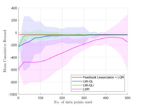
Figure 1: Mean cumulative reward and 95% confidence interval for a 100-sample simulation against the number of data points used. We compare LQR with feedback linearization, LMI-QL, LMI-QLi and LSPI.

In Fig. 1, we can observe that both proposed methods converge close to the cumulative reward that feedback linearization + LQR can achieve. We can furthermore observe that the baseline allows LMI-QL(i) to start ahead of LSPI before any data has been used. The baseline reduces the learning problem by providing a good starting for the Q-function values. Lastly, observe that the proposed methods converge faster than LSPI. This can be explained by the fact that the LSPI solution does not satisfy the $S\succ 0$ constraint at multiple points in Fig. 1, and by the fact that the proposed methods more directly learn the optimal parametrized Q-function.

V CONCLUSIONS

This paper introduces LMI-QL and LMI-QLi, two methods for direct optimal Q-function learning using convex optimization. We show that if the Q-function is parametrized in a quadratic form and if the objective function uses the $\ell_{1}$-norm of the Bellman residuals, we can derive two separate convex optimization problems. In LMI-QLi, we fix a subset of the design variables such that the optimization problem for the remaining variables becomes a semidefinite program. In LMI-QL, we relax the temporal difference minimization problem into a semi-definite program including a set of linear matrix inequalities. Simulated results indicate high data efficiency in comparison to existing methods for a nonlinear example.

Future research avenues include investigating convergence properties of LMI-QLi, and proving that the convex relaxation is exact under certain conditions.

References

- [1] R. S. Sutton and A. G. Barto, Reinforcement Learning: An Introduction, 2nd ed. MIT Press, 2018.
- [2] L. Buşoniu, D. Ernst, B. De Schutter, and R. Babuška, “Approximate reinforcement learning: An overview,” IEEE SSCI 2011: Symposium Series on Computational Intelligence - ADPRL 2011: 2011 IEEE Symposium on Adaptive Dynamic Programming and Reinforcement Learning, pp. 1–8, 2011.
- [3] L. Buşoniu, T. de Bruin, D. Tolić, J. Kober, and I. Palunko, “Reinforcement learning for control: Performance, stability, and deep approximators,” Annual Reviews in Control, vol. 46, pp. 8–28, 2018.
- [4] X. Xu, L. Zuo, and Z. Huang, “Reinforcement learning algorithms with function approximation: Recent advances and applications,” Information Sciences, vol. 261, pp. 1–31, mar 2014.
- [5] S. J. Bradtke and A. G. Barto, “Linear Least-Squares algorithms for temporal difference learning,” Machine Learning, vol. 22, no. 1-3, pp. 33–57, 1996.
- [6] M. G. Lagoudakis and R. Parr, “Least-squares policy iteration,” Journal of Machine Learning Research, vol. 4, no. 6, pp. 1107–1149, 2004.
- [7] M. G. Lagoudakis, “Least-Squares Reinforcement Learning Methods,” in Encyclopedia of Machine Learning and Data Mining. Boston, MA: Springer US, 2014, pp. 1–9.
- [8] M. Riedmiller, “Neural Fitted Q Iteration – First Experiences with a Data Efficient Neural Reinforcement Learning Method,” in Lecture Notes in Computer Science (including subseries Lecture Notes in Artificial Intelligence and Lecture Notes in Bioinformatics), 2005, vol. 3720 LNAI, pp. 317–328.
- [9] J. Schulman, F. Wolski, P. Dhariwal, A. Radford, and O. Klimov, “Proximal Policy Optimization Algorithms,” arXiv preprint arXiv:1707.06347, jul 2017.
- [10] A. Abdolmaleki, J. T. Springenberg, Y. Tassa, R. Munos, N. Heess, and M. Riedmiller, “Maximum a Posteriori Policy Optimisation,” 6th International Conference on Learning Representations, ICLR 2018 - Conference Track Proceedings, jun 2018.
- [11] V. S. Mai, D. Maity, B. Ramasubramanian, and M. C. Rotkowitz, “Convex Methods for Rank-Constrained Optimization Problems,” in 2015 Proceedings of the Conference on Control and its Applications. Philadelphia, PA: Society for Industrial and Applied Mathematics, jul 2015, pp. 123–130.