Spectral clustering of time-evolving networks using the inflated dynamic Laplacian for graphs

Abstract

Complex time-varying networks are prominent models for a wide variety of spatiotemporal phenomena. The functioning of networks depends crucially on their connectivity, yet reliable techniques for determining communities in spacetime networks remain elusive. We adapt successful spectral techniques from continuous-time dynamics on manifolds to the graph setting to fill this gap. We formulate an inflated dynamic Laplacian for graphs and develop a spectral theory to underpin the corresponding algorithmic realisations. We develop spectral clustering approaches for both multiplex and non-multiplex networks, based on the eigenvectors of the inflated dynamic Laplacian and specialised Sparse EigenBasis Approximation (SEBA) post-processing of these eigenvectors. We demonstrate that our approach can outperform the Leiden algorithm applied both in spacetime and layer-by-layer, and we analyse voting data from the US senate (where senators come and go as congresses evolve) to quantify increasing polarisation in time.

1 Introduction

Complex interconnected systems from diverse applications such as biology, economy, physical, political and social sciences can be modelled and analysed by networks [New10, BP16]. The largest impact on the functioning of most networks, by far, is due to their connectivity structure. Community detection is thus a central issue when analysing networks—or their mathematical manifestations, graphs [NG04]. In many situations, this connectivity structure and thus the underlying communities vary over time. For example, one may consider an online social network composed of vertices represented by users, and edges that represent the degree of connection between users (likes, comments, post shares, tags etc.). Communities in such a network may correspond to mutual interests or those formed by friends and family. A temporal evolution of these communities is described by changes in user interaction, essentially strengthening or weakening the edges between users as time passes, see [GDC10, BA15] for examples.

Time-evolving networks have been introduced before in the literature as multilayer networks [KAB⁺14], where the vertex set and edge weights may change over time. A special case of a multilayer network is a multiplex network, where vertices are copied across layers and each vertex maintains temporal connections only with its counterparts one layer forward and backward in time. Multilayer and multiplex networks are used to model time-varying networks where each vertex behaves as a state varying in time, and are thus ubiquitous in literature; see [MHI⁺21, RC18] for reviews on this topic. This study focuses on detecting communities in multiplex networks, as well as multilayer networks where the set of vertices themselves may change over time (see Sec. 6).

Community detection methods of multiplex networks include modularity maximisation adapted to spacetime graphs [MRM⁺10, GDC10], random walk-based approaches [KM15, KDC22], hierarchical clustering [MH19], detect-and-track methods [BA15] and ensemble methods that generalise to multilayer networks [TAG17]. In this work we prioritise the development of novel techniques for Laplacians on undirected spacetime graphs to robustly detect time-evolving spacetime communities, particularly in challenging situations where existing non-spacetime and spacetime methods fail. We do so for several reasons. First, the eigendata from graph Laplacians contain crucial information about the optimal partitioning of a graph, allowing one to relate their spectra and eigenvectors to balanced graph cuts and the resulting Cheeger constants from isoperimetric theory [Chu96a, JM85]. Second, graph Laplacians on multiplex networks, called supra-Laplacians [SRDDK⁺13, RA13, DP17], have structure that we exploit to develop theoretical justifications for the quality of spacetime communities extracted from their eigendata. Third, spectral clustering is a well-studied and robust algorithm for community detection. Spectral partitioning is computationally efficient as the resulting graph Laplacians are sparse and only require the computation of the first few eigenpairs.

Previous works have glossed over establishing results about the spectrum of supra-Laplacians [SRDDK⁺13, RA13, DP17]. We develop such spectral theory, which also justifies the performance of our spatiotemporal spectral partitioning through Cheeger constants. From this new theory we formulate a robust algorithm to detect multiple spatiotemporal clusters; our theory provides a quality guarantee of the partitions across time. Finally, we adapt our spectral partitioning approach to non-multiplex type networks, where vertices may appear and disappear in time. Our constructions to enable spectral clustering to determine several spatiotemporal clusters, as well as multilayer graphs where vertices may come and go, have to our knowledge not been formulated before.

Our constructions are inspired by the dynamic and inflated dynamic Laplacians formulated for continuous-space dynamics on manifolds [Fro15] and spacetime manifolds [FK23, AFK24], respectively. The dynamic Laplacian for graphs was formulated in [FK15]. The supra-Laplacian is the graph analogue of the inflated dynamic Laplacian, where inflation refers to expanding the graph by copying vertices across time. We refer to the supra-Laplacian as the inflated dynamic Laplacian in the sequel, to maintain consistency with similarly established notions.

Our main contributions are as follows:

1. We construct the unnormalised and normalised inflated dynamic Laplacian on graphs and state the corresponding spacetime Cheeger inequalities, which provide worst-case guarantees on clustering quality. In Prop. 2, we also prove an intuitive result concerning the monotonicity of spacetime Cheeger constants in the cardinality of the number of spacetime partition elements.

2. Vertices in individual network layers are typically connected across time with certain strengths, which can be regarded as a type of diffusion across time. We analyse the limit of increasing temporal connectivity strength, and in Thms. 4 and 5 we prove that the spectra of the unnormalised and normalised inflated dynamic Laplacians approach that of the dynamic and normalised temporal Laplacians in a hyperdiffusion limit. As a result, we gain a better understanding of how to select the appropriate diffusion constant for the inflated dynamic Laplacian for graphs, which is important for the spectral partitioning algorithm.

3. We formulate a novel spectral partitioning Algorithm 1 in conjunction with the Sparse Eigenbasis Algorithm (SEBA) [FRS19] for multiplex networks to find several spatiotemporal clusters from several spacetime eigenvectors. We illustrate the efficacy of our approach in the challenging setting of small, slowly varying networks, and demonstrate superior time-varying cluster detection when compared to (i) a spacetime application of the Leiden algorithm [TWvE19] and (ii) Leiden applied on individual time slices.

4. In Algorithm 3 we formulate a spacetime clustering procedure for non-multiplex networks, which are characterised by time-varying edge weights, and vertices that appear and disappear in time. We analyse a real-world network of voting similarities between US senators in the years 1987–2009 [MRM⁺10, WPF⁺09], and show increasing political polarisation over recent decades.

An outline of the paper is as follows. We begin with a simple motivating example of a multiplex network with 5 vertices and 5 time slices in Sec. 1.1 that captures many of the fundamental ideas of our approach. We formulate the main spacetime constructions in Sec. 2. In Sec. 3 we analyse the spectral structure of the inflated dynamic Laplacian and prove spectral results in the hyperdiffusion limit. Our spectral partitioning algorithm is formulated in Sec. 4. In Sec. 5 we demonstrate the algorithm on two model networks. Finally in Sec. 6 we adapt the spectral partitioning algorithm to non-multiplex networks and apply it to detect communities in a real world network of voting similarities in the US Senate. A Julia implementation of the algorithms and the examples presented here can be found at https://github.com/mkalia94/TemporalNetworks.jl.

1.1 Motivating example

The first purpose of this example is to highlight how a spatiotemporal Laplacian construction is able to identify evolving clusters together with the times of their (partial) appearance and disappearance in evolving networks. Its second purpose is to informally introduce the main objects that support our theoretic and algorithmic constructions.

Consider the spacetime network as presented in Fig. 1.

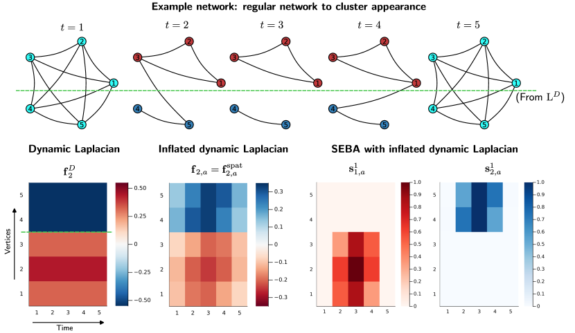
Figure 1: Comparing spectral partitioning methods to discover communities in spacetime graphs. Upper: spacetime graph/ multiplex network composed of 5 time slices with 5 vertices each. As time progresses, a cluster composed of vertices $\{1,2,3\}$ appears from a 4-regular graph before returning to the regular graph. Lower left: The second eigenvector $\mathrm{f}^{D}_{2}=[0.324,0.442,0.324,-0.545,-0.545]^{\top}$ of the dynamic Laplacian (copied across time to create a spacetime vector $\bm{\mathrm{f}}_{2}^{D}$) reveals a partition, demarcated by green dashed line, and is composed of vertices $\{1,2,3\}$ and $\{4,5\}$ respectively. This partition remains the same for all time, and does not reveal the appearing and disappearing of the red and dark blue clusters in the network. Lower right: The SEBA algorithm (Algorithm 1 - step 5) applied to the second eigenvector $\bm{\mathrm{f}}_{2,a}$ (in this case equal to the first spatial eigenvector $\bm{\mathrm{f}}^{\rm spat}_{2,a}$) of the inflated dynamic Laplacian yields two vectors ${\bm{\mathrm{s}}}_{1,a}^{1}$ and ${\bm{\mathrm{s}}}_{2,a}^{1}$ that reveals the emergence of two disjoint clusters at time $t=2$ and their disappearance after $t=4$. Note that the 4-regular graphs at times $t=1$ and $t=5$ are not partitioned because they contain no clusters.

The network is composed of 5 vertices for each of the 5 time slices. Each edge has a weight that switches between zero and one arbitrarily as time progresses. At time $t=3$, a separate community composed of the set of vertices $\{1,2,3\}$ appears, then disappears with the return of the regular graph at $t=5$. The goal is then to discover the community represented by vertices $\{1,2,3\}$ (and thus also vertices $\{4,5\}$) at times $t=2,3,4$. Let $W=\{\mathrm{W}^{(1)},\dots,\mathrm{W}^{(5)}\}$ be the collection of adjacency matrices for each time slice; see the black lines in Fig. 1 (upper).

Persistent communities: In [FK15] the dynamic Laplacian for graphs subjected to vertex permutations was introduced as a method to detect persistent communities in spacetime graphs. Define the average adjacency $\mathrm{W}^{D}:=\frac{1}{5}\sum_{i}\mathrm{W}^{(i)}$. The dynamic Laplacian $\mathrm{L}^{D}$ is the (unnormalised) Laplacian for the weights $\mathrm{W}^{D}$. Spectral partitioning is then performed on $\mathrm{L}^{D}$. The first eigenvector of $\mathrm{L}^{D}$ corresponding to eigenvalue $0$ is simply $\mathrm{f}^{D}_{1}=[1,\dots,1]^{\top}$. Using a zero threshold on the second eigenvector $\mathrm{f}^{D}_{2}=[0.324,\ 0.442,\ 0.324,\ -0.545,\ -0.545]^{\top}$ reveals the underlying partition composed of vertices $\{1,2,3\}$ and $\{4,5\}$, which is indeed the optimal fixed-in-time cut for this spacetime graph (green dashed line in Fig. 1 (lower left)).

Evanescent communities: A fixed-in-time partition cannot reveal the full temporal connectivity information of the spacetime graph. We seek communities that are present for substantial portions of time, but do not necessarily persist through the entire time duration. To capture such transient communities we use the graph Laplacian constructed on a spacetime graph with temporal diffusion along the temporal arcs. In the literature, such a construction has been called a supra-Laplacian [GDGGG⁺13, SRDDK⁺13]. We will call it inflated dynamic Laplacian, because of its strong relations to the dynamic Laplacian, which we discuss in Thm. 4 below.

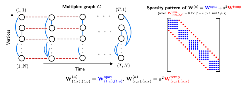
Figure 2: The multiplex network framework. (Left) A spacetime graph $\bm{G}$ with time/layers in the horizontal direction and vertices within each time slice/layer in the vertical direction. The connections form the adjacency $\bm{\mathrm{W}}^{(a)}$ which can be split into blue spatial ($\bm{\mathrm{W}}^{\rm spat}$) and red temporal ($a^{2}\bm{\mathrm{W}}^{\rm temp}$) components respectively. (Right) Sparsity pattern of the matrix representation of $\bm{\mathrm{W}}^{(a)}$ with respect to the ordering (32).

A simple example of temporal diffusion is diffusion to nearest neighbours in time. The corresponding temporal Laplacian is

$$\mathrm{L}^{\mathrm{temp}}=\left[\begin{array}[]{ccccc}1&-1&0&0&0\\ -1&2&-1&0&0\\ 0&-1&2&-1&0\\ 0&0&-1&2&-1\\ 0&0&0&-1&1\\ \end{array}\right].$$ (1)

Defining $\mathrm{L}^{(i)}$ to be the (unnormalised) Laplacian for the weights $\mathrm{W}^{(i)}$, we define by $\bm{\mathrm{L}}^{(a)}$ the inflated dynamic Laplacian of the spacetime graph shown in Fig. 1 (upper), where the boldface indicates the spacetime nature of the matrix. The inflated dynamic Laplacian $\bm{\mathrm{L}}^{(a)}$ is given by

$$\bm{\mathrm{L}}^{(a)}=\mathrm{blockdiag}(\mathrm{L}^{(1)},\ldots,\mathrm{L}^{(5)})+a^{2}(\mathrm{L}^{\rm temp}\otimes\mathrm{I}),$$ (2)

where the parameter $a>0$ weights the contributions of the temporal component relative to the spatial components. Here, $\otimes$ denotes the Kronecker product of matrices (cf. (38)) and $\mathrm{I}$ the identity matrix. With the “space-first” ordering of the multiplex (spacetime) network’s vertices as in Fig. 2 (upper left), the inflated dynamic Laplacian $\bm{\mathrm{L}}^{(a)}$ and its weight matrix $\bm{\mathrm{W}}^{(a)}$ both have the sparsity structure shown in Fig. 2 (upper right). In this example we choose $a=2$ to appropriately scale spatial and temporal components (see Algorithm 1 for details). We now perform spectral partitioning on the inflated dynamic Laplacian. As in the dynamic case, the first eigenvector is simply $\bm{\mathrm{f}}_{1,a}=[1,\dots,1]^{\top}$. The second eigenvector $\bm{\mathrm{f}}_{2,a}$ indicates the spacetime partition. To create the spacetime partition we apply the SEBA algorithm [FRS19] to two vectors constructed from $\bm{\mathrm{f}}_{2,a}$ (see Algorithm 1) which returns two vectors $\smash{\bm{\mathrm{s}}_{(1,2),a}^{1}}$ containing the clusters $\{1,2,3\}$ and $\{4,5\}$ separately, at times $t=2,3,4$, seen in Fig. 1 (lower left). This example shows that appearance and disappearance of communities (in time) can be extracted by spacetime spectral computations.

2 Spacetime graphs

The spectral study of time-evolving networks requires extensive notation. To help the reader navigate this notation we list some typical examples in Table 1. Time-evolving networks have nodes indexed by both space and time. Generally, we distinguish spacetime objects from purely spatial or purely temporal objects by denoting the former by boldface symbols. Further, operators are calligraphic, matrices are upper case upright (roman), functions are italic, vectors are lower case upright, sets are upper case italic, and partitions of sets are fraktur letters. Scalars, indices, nodes in graphs, and other objects have a standard notation that is not synchronised with the previous choices, but their identification should be clear from the context. For instance, $a$ will always be a scalar and never a function.

object type	space or time object	spacetime object
operator	$\mathcal{W},\mathcal{L}$	$\bm{\mathcal{W}},\bm{\mathcal{L}}$
matrix	$\mathrm{W}^{(i)},\mathrm{L}^{D}$	$\bm{\mathrm{L}}^{(a)}$
function	$f^{D}$	$\bm{f}_{2,a}$
vector	$\mathrm{f}^{\mathrm{temp}}$	$\bm{\mathrm{s}}_{1}$
set	$V^{\prime}$	$\bm{X}_{k}$
partition	$\mathfrak{X}$	$\bm{\mathfrak{X}}$
Cheeger ratio/const.	$H_{K}/h_{K}$	$\bm{H}_{K}/\bm{h}_{K}$
eigenvalues	$\lambda_{k}$	$\bm{\lambda}_{k}$

Table 1: Reference table with examples of notation.

We distinguish operators and functions on graphs from matrices and vectors representing them, both to align with existing literature and to draw the line between an intuitive, intrinsic description of objects (in terms of vertices and edges) and their representations for algorithms that use a specific enumeration of the vertices.

2.1 Spacetime graphs and clusters

Let $G=(V,E,\mathcal{W})$ be a general undirected graph with finite sets of vertices $V\subset\mathbb{N}$ and edges $(x,y)\in E$ for vertices $x,y\in V$. The function $\mathcal{W}:V\times V\to\mathbb{R}_{0}^{+}$ assigns weights to the edges such that $\mathcal{W}(x,y)>0$ and is symmetric in arguments. The degree $d(x)$ of a vertex $x$ is given by $d(x)=\sum_{y}\mathcal{W}(x,y)$.

We now extend these definitions to spacetime graphs. Let $V=\{1,\dots,N\}$ denote the spatial vertex set and $V^{\prime}=\{1,\dots,T\}$ be the temporal vertex set for finite $N,T\in\mathbb{N}$. We define the spacetime vertex set $\bm{V}=V^{\prime}\times V$ which gives rise to the spacetime, multiplex graph $\bm{G}$ defined by the tuple $\bm{G}=(\bm{V},\bm{E},\bm{\mathcal{W}}^{(a)})$ where $\bm{E}$ is the edge set connecting vertices $\bm{V}$ defined as follows,

$$\bm{E} =\{((t,x),(s,y))\ |\ (t,x)\sim(s,y)\ \textnormal{in }\bm{G}\}.$$

The notation $(t,x)\sim(s,y)$ denotes a connection between vertices $(t,x)$ and $(s,y)$ in $\bm{G}$. For every graph $\bm{G}$ we associate a weight function $\bm{\mathcal{W}}^{(a)}$ parameterised by $a>0$ such that $\smash{\bm{\mathcal{W}}^{(a)}_{(t,x),(s,y)}\in\mathbb{R}^{+}_{0}}$ is the weight of the edge joining the vertices $(t,x)$ and $(s,y)$. We decompose $\bm{\mathcal{W}}^{(a)}$ into $\bm{\mathcal{W}}^{\rm spat}$ and $a^{2}\bm{\mathcal{W}}^{\rm temp}$, the spatial and temporal components of $\bm{\mathcal{W}}^{(a)}$, so that

$$\bm{\mathcal{W}}^{(a)}=\bm{\mathcal{W}}^{\rm spat}+a^{2}\bm{\mathcal{W}}^{\rm temp},$$ (3)

and

$$\bm{\mathcal{W}}^{\rm spat}_{(t,x),(s,y)} =0,\ t\neq s,$$

$$\bm{\mathcal{W}}^{\rm temp}_{(t,x),(s,y)} =0,\ x\neq y.$$ (4)

We further restrict $\bm{\mathcal{W}}^{\rm temp}$ so that it is space-independent, i.e.,

$$\bm{\mathcal{W}}^{\rm temp}_{(t,x),(s,x)}=\bm{\mathcal{W}}^{\rm temp}_{(t,y),(s,y)}=:\mathcal{W}^{\prime}_{t,s}\textnormal{ for all $t,s,x,y$}.$$ (5)

Clustering spacetime graphs.

Individual clusters are of spacetime type and can thus emerge, split, merge or disappear as time passes. For clarity, we formally define these transitions below. When discussing clustering we will use the notion of packing which is more general than partitioning. A $K$-packing $\bm{\mathfrak{X}}=\{\bm{X}_{1},\ldots,\bm{X}_{K}\}$ of the vertex set $\bm{V}$ is defined by a collection of disjoint subsets $\bm{X}_{i}\subset\bm{V}$, $1\leq i\leq K$. The $K$-packing $\bm{\mathfrak{X}}$ can be one of two possible types: (i) fully clustered, where $\bm{\mathfrak{X}}$ partitions $\bm{V}$ or (ii) partially clustered, where $\bigcup_{k=1}^{K}\bm{X}_{k}\subsetneq\bm{V}$. In this latter case, we denote the unclustered vertices by $\bm{\Omega}=\bm{V}\setminus\bigcup_{k=1}^{K}\bm{X}_{k}$.

Example.

In Fig. 1, we have $\bm{\mathfrak{X}}=\{\bm{\Omega},\bm{X}_{1},\bm{X}_{2}\}$, where

$$\bm{\Omega}=\{(1,1),(1,2),(1,3),(1,4),(1,5),(5,1),(5,2),(5,3),(5,4),(5,5)\},$$

$$\bm{X}_{1}=\{(2,1),(2,2),(2,3),(3,1),(3,2),(3,3),(4,1),(4,2),(4,3)\},$$

$$\mbox{and }\bm{X}_{2}=\{(2,4),(2,5),(3,4),(3,5),(4,4),(4,5)\}.$$

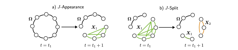
Figure 3: Two typical cluster/partition transitions: a) $J$-appearance (for $J=2$) where cluster $\bm{X}_{1}$ appears from the unclustered set $\bm{\Omega}$ and b) $J$-split (for $J=2$), where a cluster $\bm{X}_{2}$ splits from an existing cluster $\bm{X}_{1}$.

The splitting and appearance of a cluster in our spacetime setting is defined as follows:

1. $J$-split: For $J\geq 2$, a cluster $\bm{X}_{k}$ is said to $J$-split from time $t$ to $t+1$ if there is a collection $\bm{J}\subset\{\bm{X}_{1},\ldots,\bm{X}_{K}\}$ (fully clustered case) or $\bm{J}\subset\{\bm{\Omega},\bm{X}_{1},\dots,\bm{X}_{K}\}$ (partially clustered case) with $|\bm{J}|=J$ and $\bm{X}_{k}\in\bm{J}$ such that

   $$\left\{x\in V\,:\,(t,x)\in\bm{X}_{k}\right\}=\left\{x\in V\,:\,(t+1,x)\in\textstyle{\bigcup_{\bm{X}\in\bm{J}}}\bm{X}\right\}.$$ (6)

   In words, the space nodes in $\bm{X}_{k}$ at time $t$ now lie in the union of $J$ packing elements at time $t+1$. If $\bm{X}_{k}$ undergoes a 2-split from time $t$ to $t+1$ with $\bm{J}=\{\bm{\Omega},\bm{X}_{k}\}$, this corresponds to $\bm{X}_{k}$ shrinking.

2. $J$-appearance:

   1. For $J\geq 1$, a cluster $\bm{X}_{k}$ is said to cause a $J$-appearance from time $t$ to $t+1$ if $\bm{X}_{k}$ fulfils all of the conditions for a $J$-split from time $t$ to $t+1$, except that $\bm{X}_{k}\notin\bm{J}$. In words, the space nodes in $\bm{X}_{k}$ at time $t$ are reassigned to $J$ other clusters at time $t+1$, possibly with an additional unclustered set $\bm{\Omega}$.

   2. For $J\geq 2$, the unclustered set $\bm{\Omega}$ is said to cause a $J$-appearance if $\bm{\Omega}$ undergoes a $J$-splitting from time $t$ to $t+1$, where $\bm{\Omega}$ may or may not be an element of $\bm{J}$. In words, the space nodes in the unclustered set at time $t$ give rise to $J$ clustered sets at time $t+1$, with some space nodes possibly remaining unclustered.

“$J$-merge” and “$J$-disappearance” are defined analogously, by swapping the roles of $t$ and $t+1$.

Example (cont…).

In Fig. 1 the graph undergoes a 2-appearance at $t=1$, where all space nodes $\{1,2,3,4,5\}$ in $\bm{\Omega}$ at $t=1$ are reassigned to space nodes in the clusters $\bm{X}_{1},\bm{X}_{2}$ at time $t=2$. Similarly, the graph in Fig. 1 undergoes a 2-disappearance at $t=4$, where the space nodes in the clusters $\bm{X}_{1},\bm{X}_{2}$ are all reassigned to $\bm{\Omega}$ at time $t=5$. See also the explicit element listings for $\bm{\Omega},\bm{X}_{1},\bm{X}_{2}$ in the Example immediately above.

2.2 Laplacians of spacetime graphs

From [Chu96b], the unnormalised and normalised graph Laplacians for general graphs are defined as follows. The unnormalised graph Laplacian $\mathcal{L}$ acts on functions $f:V\to\mathbb{R}$ and is given by

$$\mathcal{L}f(x)=\sum_{y}\mathcal{W}(x,y)\left(f(x)-f(y)\right).$$ (7)

The corresponding normalised Laplacian $\overline{\mathcal{L}}$ is given by

$$\overline{\mathcal{L}}f(x)=\sum_{y}\mathcal{W}(x,y)\left(\frac{f(x)}{d(x)}-\frac{f(y)}{d(x)^{1/2}d(y)^{1/2}}\right).$$ (8)

We extend these definitions to the spacetime case. First, we define by $\bm{d}^{(a)}$, $\bm{d}^{\rm spat}$ and $\bm{d}^{\rm temp}$ the degree functions over vertices $(t,x)\in\bm{V}$ and subsets of vertices $\bm{X}\subset\bm{V}$. The expressions are as follows:

$$\bm{d}^{(a)}(t,x) =\sum_{(s,y)\in\bm{V}}\bm{\mathcal{W}}^{(a)}_{(t,x),(s,y)}, \bm{d}^{(a)}(\bm{X}) =\sum_{(t,x)\in\bm{X}}\bm{d}^{(a)}(t,x),$$

$$\bm{d}^{\rm spat}(t,x) =\sum_{y\in\bm{V}}\bm{\mathcal{W}}^{\rm spat}_{(t,x),(t,y)}, {\bm{d}^{\rm spat}}(\bm{X}) =\sum_{(t,x)\in\bm{X}}\bm{d}^{\rm spat}(t,x),$$

$$\bm{d}^{\rm temp}(t,x) =\sum_{s\in V^{\prime}}\bm{\mathcal{W}}^{\rm temp}_{(t,x),(s,y)}, {\bm{d}^{\rm temp}}(\bm{X}) =\sum_{(t,x)\in\bm{X}}\bm{d}^{\rm temp}(t,x).$$ (9)

Note that by (5), $\bm{d}^{\rm temp}(t,x)=\sum_{s\in V^{\prime}}\mathcal{W}^{\prime}_{t,s}$ and is therefore independent of $x$. Thus we use $d^{\rm temp}(t)$ in the rest of the paper. On the graph $\bm{G}$ equipped with weights $\bm{\mathcal{W}}^{(a)}$, we define the unnormalised graph inflated dynamic Laplacian $\bm{\mathcal{L}}^{(a)}$ as an operator acting on functions $\bm{f}:\bm{V}\to\mathbb{R}$ as

$$\bm{\mathcal{L}}^{(a)}\bm{f}(t,x):=\sum_{(s,y)\in\bm{V}}\bm{\mathcal{W}}^{(a)}_{(t,x),(s,y)}\left(\bm{f}(t,x)-\bm{f}(s,y)\right).$$ (10)

We define the normalised graph inflated dynamic Laplacian $\overline{\bm{\mathcal{L}}^{(a)}}$ acting on functions $\bm{f}:\bm{V}\to\mathbb{R}$ as

$$\overline{\bm{\mathcal{L}}^{(a)}}\bm{f}(t,x):=\sum_{(s,y)\in\bm{V}}\bm{\mathcal{W}}^{(a)}_{(t,x),(s,y)}\left(\frac{\bm{f}(t,x)}{\bm{d}^{(a)}(t,x)}-\frac{\bm{f}(s,y)}{\bm{d}^{(a)}(t,x)^{1/2}\bm{d}^{(a)}(s,y)^{1/2}}\right).$$ (11)

We note that in the case of the normalised inflated dynamic Laplacian, the corresponding graph $\bm{G}$ should not contain isolated vertices in order to make sure $\bm{d}^{(a)}(t,x)>0$, $\forall(t,x)\in\bm{V}$. As the operator ${\bm{\mathcal{L}}}^{(a)}$ is linear in the argument $\bm{\mathcal{W}}^{(a)}$, we decompose ${\bm{\mathcal{L}}}^{(a)}$ similarly to $\bm{\mathcal{W}}^{(a)}$ in (3) as,

$$\bm{\mathcal{L}}^{(a)}={\bm{\mathcal{L}}}^{\rm spat}+a^{2}{\bm{\mathcal{L}}}^{\rm temp},$$ (12)

where

$${\bm{\mathcal{L}}}^{\rm spat}\bm{f}(t,x) =\sum_{y\in\bm{V}}\bm{\mathcal{W}}^{\rm spat}_{(t,x),(t,y)}\left(\bm{f}(t,x)-\bm{f}(t,y)\right),$$ (13)

$${\bm{\mathcal{L}}}^{\rm temp}\bm{f}(t,x) =\sum_{s\in V^{\prime}}\bm{\mathcal{W}}^{\rm temp}_{(t,x),(s,x)}\left(\bm{f}(t,x)-\bm{f}(s,x)\right).$$

For now it is sufficient to note that by construction all graph Laplacians considered here are self-adjoint (with respect to different inner products), positive semidefinite, and hence have purely real nonnegative spectrum. The standard inner product for real vectors (or equivalently, for functions) $f,g$ will be denoted by $\langle f,g\rangle$. This inner product notation will be used in several scenarios, but to which spaces $f$ and $g$ belong will always be clear from the context.

Definition 1.

For $a\geq 0$ and $k=1,2,\ldots,TN$, we denote the $k$-th eigenpair (in ascending order) of ${\bm{\mathcal{L}}}^{(a)}$ by $({\bm{\lambda}}_{k,a},{\bm{f}}_{k,a})$ and the $k$-th eigenpair of $\smash{\overline{\bm{\mathcal{L}}^{(a)}}}$ by $(\overline{\bm{\lambda}}_{k,a},\overline{\bm{f}}_{k,a})$.

Finally we mention the dynamic Laplacian operator [FK15] $\mathcal{L}^{D}$ acting on functions $f:V\to\mathbb{R}$. It is derived by first averaging the spatial adjacency $\bm{\mathcal{W}}^{\rm spat}$ over the time fibers to obtain $\mathcal{W}^{D}$, indexed as follows:

$$\mathcal{W}^{D}_{x,y}:=\frac{1}{T}\sum_{t\in V^{\prime}}\bm{\mathcal{W}}^{\rm spat}_{(t,x),(s,y)}=\frac{1}{T}\sum_{t\in V^{\prime}}\bm{\mathcal{W}}^{(a)}_{(t,x),(t,y)}.$$ (14)

Consider the graph $G^{D}=(V,E,\mathcal{W}^{D})$ with edges from the set $E$ connecting vertices in $V$ and define the average degree $d^{D}(x)$ by

$${d^{D}}(x):=\frac{1}{T}\sum_{t\in V^{\prime}}\bm{d}^{\rm spat}(t,x).$$ (15)

Then the unnormalised dynamic Laplacian $\mathcal{L}^{D}$ acts over functions $f:V\to\mathbb{R}$ and is given by

$$\mathcal{L}^{D}f(x):=\sum_{y\in V}\mathcal{W}^{D}_{x,y}\left(f(x)-f(y)\right).$$ (16)

2.3 Graph cuts in spacetime

We define the (edge) cut value $\bm{\sigma}(\bm{X})$ between a subset $\bm{X}\subset\bm{V}$ and its complement $\bm{X}^{\complement}\equiv\bm{V}\setminus\bm{X}$ by

$$\bm{\sigma}(\bm{X}):=\sum_{(t,x)\in\bm{X}}\sum_{(s,y)\in\bm{X}^{\complement}}\bm{\mathcal{W}}^{(a)}_{(t,x),(s,y)}\,.$$ (17)

We think of clusters being “good” if their cut values are low. For the graph $\bm{G}=(\bm{V},\bm{E},\bm{\mathcal{W}}^{(a)})$, we are interested in the balanced graph cut problem. We consider a $K$-packing $\bm{\mathfrak{X}}=\{\bm{X}_{1},\dots,\bm{X}_{K}\}$ of the spacetime vertex set $\bm{V}$, such that $\bm{X}_{k}\cap\bm{X}_{l}=\emptyset$, $\forall k\neq l$. The goal is to minimise $\max_{k\in\{1,\dots,K\}}\bm{\sigma}(\bm{X}_{k})$ produced by such a packing while making sure that the node count or degree of each individual $\bm{X}_{k}$ is as large as possible. The standard quantity to minimise over the $K$-packing $\bm{\mathfrak{X}}$ are the unnormalised and normalised Cheeger functions $\bm{H}(\bm{X}_{k})$ and $\overline{\bm{H}}(\bm{X}_{k})$ defined by

$$\bm{H}(\bm{X}):=\frac{\bm{\sigma}(\bm{X})}{|{\bm{X}}|},\quad\overline{\bm{H}}(\bm{X}):=\frac{\bm{\sigma}(\bm{X})}{\bm{d}^{(a)}(\bm{X})}.$$ (18)

Denote $\bm{H}_{K}(\bm{\mathfrak{X}}):=\max_{1\leq k\leq K}\bm{H}(\bm{X}_{k})$. The unnormalised Cheeger constant $\bm{h}_{K}$ is given by

$$\bm{h}_{K}:=\min_{\bm{\mathfrak{X}}\text{ is a $K$-packing of }\bm{V}}\bm{H}_{K}(\bm{\mathfrak{X}}) =\min_{\bm{X}_{1},\dots,\bm{X}_{K}}\max_{1\leq k\leq K}\bm{H}(\bm{X}_{k})$$ (19)

$$=\min_{\bm{X}_{1},\dots,\bm{X}_{K}}\max_{1\leq k\leq K}\frac{\bm{\sigma}(\bm{X}_{k})}{|{\bm{X}_{k}}|}.$$

Similarly, denote $\overline{\bm{H}}_{K}(\bm{\mathfrak{X}}):=\max_{1\leq k\leq K}\overline{\bm{H}}(\bm{X}_{k})$. The normalised Cheeger constant $\overline{\bm{h}}_{K}$ is given by

$$\overline{\bm{h}}_{K}:=\min_{\bm{\mathfrak{X}}\text{ is a $K$-packing of }\bm{V}}\overline{\bm{H}}_{K}(\bm{\mathfrak{X}}) =\min_{\bm{X}_{1},\dots,\bm{X}_{K}}\max_{1\leq k\leq K}\overline{\bm{H}}(\bm{X}_{k})$$ (20)

$$=\min_{\bm{X}_{1},\dots,\bm{X}_{K}}\max_{1\leq k\leq K}\frac{\bm{\sigma}(\bm{X}_{k})}{\bm{d}^{(a)}({\bm{X}_{k}})}.$$

In the case $K=2$ in (20) we have the celebrated Cheeger inequality [Chu96b] relating the normalised Cheeger constant and the spectral gap of the normalised Laplacian:

$$\overline{\bm{h}}_{2}\leq\sqrt{2\overline{\bm{\lambda}}_{2,a}}\,.$$ (21)

We state a result about the monotonicity of $\bm{h}_{K}$ in $K$, which is useful for making comparisons between differently sized packings/partitions produced by clustering algorithms.

Proposition 2.

For $K\in\mathbb{N}$ we have,

$$\overline{\bm{h}}_{K} \leq\overline{\bm{h}}_{K+1},$$ (22)

$${\bm{h}}_{K} \leq{\bm{h}}_{K+1}.$$

Proof.

See Appendix A. ∎

For general $K$, we recall the following result for the $K$-th smallest eigenvalue $\smash{\overline{\bm{\lambda}}_{K,a}}$ of $\smash{\overline{\bm{\mathcal{L}}^{(a)}}}$, which follows directly from [LGT14, Thm. 4.9]. For a graph $G$ and given $\delta\in(0,1)$, there exists a $K^{\prime}$-packing $\{X_{1},\dots,X_{K^{\prime}}\}$, $X_{i}\cap X_{j}=\emptyset$, $\forall i\neq j$ for some $K^{\prime}\geq\lceil(1-\delta)K\rceil$ such that $\smash{\overline{h}_{K^{\prime}}\leq CK^{1/2}\delta^{-3/2}(\overline{\lambda}_{K,a})^{1/2}}$ for some constant $C$ depending on the graph but independent of the packing. By choosing $\delta=1/2K$ we have that $K^{\prime}\geq K$ and using Proposition 2 we obtain

$$\overline{\bm{h}}_{K}\leq\overline{\bm{h}}_{K^{\prime}}\leq 2^{3/2}CK^{2}\sqrt{\overline{\bm{\lambda}}_{K,a}}\,.$$ (23)

For reasons to be discussed in Sec. 3 we will focus on the unnormalised Laplacian $\bm{\mathcal{L}}^{(a)}$ in the following and in particular in the numerical investigations below. However, Cheeger inequalities involving the unnormalised Cheeger constant $\bm{h}_{K}$ and the unnormalised Laplacian $\bm{\mathcal{L}}^{(a)}$ are less developed than their normalised counterparts, which we have just discussed. From [KM16, Thm. 3.1] we know that for a graph $G=(V,E)$ equipped with adjacency $\mathcal{W}$ and an unnormalised Laplacian $\mathcal{L}$ with corresponding $k$-th eigenvalue $\lambda_{k}$ we have the Cheeger inequality $h_{2}\leq\sqrt{2\lambda_{2}\max_{x}d(x)}$ where $d(x)=\sum_{y\in V}\mathcal{W}_{x,y}$. Thus, for $K=2$ we have the following:

$$\bm{h}_{2}\leq\sqrt{2\bm{\lambda}_{2,a}\max_{(t,x)}\bm{d}^{(a)}(t,x)}.$$ (24)

To compare the relative tightness of (24) and (21), let us briefly assume that the degrees are constant, say, $\bm{d}^{(a)}(x,t)\equiv d$. Then we see that $\bm{h}_{K}=d\,\overline{\bm{h}}_{K}$ and $\smash{\bm{\mathcal{L}}^{(a)}=d\,\overline{\bm{\mathcal{L}}^{(a)}}}$, the latter implying $\bm{\lambda}_{a,K}=d\,\overline{\bm{\lambda}}_{a,K}$. The unnormalised Cheeger inequality (24) in this case becomes $\bm{h}_{2}\leq\sqrt{2\bm{\lambda}_{2,a}d}$, which is—by the equations listed in the previous sentence—equivalent to the Cheeger inequality (21) in the normalised case. We thus expect the performance guarantee given by the unnormalised Cheeger inequality to be as strong as the one from the normalised case, as long as the relative variation in degrees is not too large.

3 Eigenvalues of inflated dynamic Laplacians and the hyperdiffusion limit

The graph cuts defined in the previous section critically depend on the eigenvalues of the associated inflated dynamic Laplacians. The eigenvectors of the (un)-normalised inflated dynamic Laplacian are used ahead to perform spectral partitioning of the spacetime graph to detect persistent communities. The inflated dynamic Laplacian depends on the parameter $a$, which scales the contribution of the spatial and temporal components. We show in Thm. 4 that a few of the eigenvalues(vectors) of the corresponding unnormalised inflated dynamic Laplacian $\smash{{\bm{\mathcal{L}}}^{(a)}}$ approach that of the corresponding unnormalised dynamic Laplacian $\smash{{\mathcal{L}^{D}}}$ as $a\to\infty$. For the normalised Laplacian $\smash{\overline{\bm{\mathcal{L}}^{(a)}}}$, the eigenvalues approach that of the normalised temporal Laplacian $\overline{\bm{\mathcal{L}}^{\rm temp}}$ as $a\to\infty$, as shown in Thm. 5.

3.1 The unnormalised Laplacian $\bm{\mathcal{L}}^{(a)}$

Let $G^{\prime}=(V^{\prime},E^{\prime},\mathcal{W}^{\prime})$ be such that $\mathcal{W}^{\prime}$ is defined in (5). The vertices $V^{\prime}=\{1,\ldots,T\}$ and $t\sim s\textnormal{ in }E^{\prime}\iff\mathcal{W}^{\prime}_{t,s}\neq 0$. Let $\mathcal{L}^{\prime}$ be the corresponding graph Laplacian. We denote the $k$-th eigenpair of $\mathcal{L}^{\prime}$ by $(\lambda_{k}^{\rm temp},f_{k}^{\rm temp})$. The $TN$ eigenpairs $\{(\bm{\lambda}_{1,a},\bm{f}_{1,a}),\ldots,(\bm{\lambda}_{TN,a},\bm{f}_{TN,a})\}$ of ${\bm{\mathcal{L}}}^{(a)}$ can be split into two collections: temporal $\{(\bm{\lambda}^{\rm temp}_{2,a},\bm{f}^{\rm temp}_{2,a}),\ldots,(\bm{\lambda}^{\rm temp}_{T,a},\bm{f}^{\rm temp}_{T,a})\}$ and spatial $\smash{\{(\bm{\lambda}^{\rm spat}_{1,a},\bm{f}^{\rm spat}_{1,a}),\ldots,(\bm{\lambda}^{\rm spat}_{TN-T+1,a},\bm{f}^{\rm spat}_{TN-T+1,a})\}}$.

Lemma 3 (Spatial and temporal eigenpairs of ${\bm{\mathcal{L}}}^{(a)}$).

The eigenpairs of ${\bm{\mathcal{L}}}^{(a)}$ are classified as follows:

1. $T-1$ temporal eigenvalues ${\bm{\lambda}}_{k,a}^{\rm temp}$, which satisfy ${\bm{\lambda}}_{k,a}^{\rm temp}=a^{2}\lambda_{k}^{\rm temp}$, $2\leq k\leq T$. Corresponding to these temporal eigenvalues are $T-1$ temporal eigenfunctions $\smash{{\bm{f}}_{k,a}^{\rm temp}}$, which satisfy ${\bm{f}}_{k,a}^{\rm temp}(t,x)=f_{k}^{\rm temp}(t)$, $2\leq k\leq T$.

2. $TN-T+1$ spatial eigenvalues ${\bm{\lambda}}_{k,a}^{\rm spat}$. Corresponding to these spatial eigenvalues are $TN-T+1$ spatial eigenfunctions ${\bm{f}}_{k,a}^{\rm spat}$. For each $1\leq k\leq TN-N+1$, there is a constant $C_{k}$ such that $\sum_{x\in V}{\bm{f}}_{k,a}^{\rm spat}(t,x)=C_{k}$ for all $1\leq t\leq T$.

Proof.

See Appendix B. ∎

By convention we consider $\bm{\lambda}_{1,a}$ to be spatial eigenvalue; this is consistent with Thm. 4 and previous work [FK23]. We now show in Thm. 4 that the first $N$ spatial eigenvalues and eigenvectors approach those of the dynamic Laplacian [FK15] in the hyperdiffusion limit, i.e. as $a\to\infty$. Part 3 of Thm. 4 appeared in [SRDDK⁺13]; we prove the theorem using a variational approach, which in comparison to [SRDDK⁺13] results in a stronger statement about the behaviour of $\bm{\lambda}_{k,a}$ and $\bm{f}_{k,a}$ and generalises to different forms of $\mathcal{W}^{\prime}$. Note that the spectrum $\bm{\sigma}_{a}$ of ${\bm{\mathcal{L}}}^{(a)}$ is given by $\smash{\bm{\sigma}_{a}=\bigcup_{k}{\bm{\lambda}}^{\rm spat}_{k,a}\cup\bigcup_{k}{\bm{\lambda}}^{\rm temp}_{k,a}}$ for spatial eigenvalues ${\bm{\lambda}}^{\rm spat}_{k,a}$ and temporal eigenvalues ${\bm{\lambda}}^{\rm temp}_{k,a}$. Ordering the eigenvalues ${\bm{\lambda}}_{k,a}$ of ${\bm{\mathcal{L}}}^{(a)}$ as ${\bm{\lambda}}_{1,a}\leq{\bm{\lambda}}_{2,a}\leq\dots$, we obtain the trivial inequalities,

$${\bm{\lambda}}_{k,a}\leq{\bm{\lambda}}_{k,a}^{\rm spat}{\mbox{ for $1\leq k\leq TN-N-1$, and }}\ \ {\bm{\lambda}}_{k,a}\leq{\bm{\lambda}}_{k,a}^{\rm temp}{\mbox{ for $2\leq k\leq T$}}.$$ (25)

Theorem 4 (Hyperdiffusion limit of ${\bm{\mathcal{L}}}^{(a)}$).

Let $\bm{G}=(\bm{V},\bm{E},\bm{\mathcal{W}}^{(a)})$ be a spacetime graph and let ${\bm{\lambda}}_{k,a},k=1,\ldots,TN,$ be the eigenvalues of the unnormalised inflated dynamic Laplacian ${\bm{\mathcal{L}}}^{(a)}$. Let ${\lambda}_{k}^{D}$, $k=1,\ldots,N$, denote the eigenvalues of the corresponding dynamic Laplacian ${\mathcal{L}^{D}}$. Then the following statements hold:

1. $\bm{\lambda}_{k,a}\leq\lambda_{k}^{D}$, for $1\leq k\leq N$.

2. $\bm{\lambda}_{k,a}$ is nondecreasing for increasing $a$, for $1\leq k\leq TN$.

3. $\lim_{a\rightarrow\infty}{\bm{\lambda}}_{k,a}={\lambda}_{k}^{D}$, for $1\leq k\leq N$.

4. The accumulation points of the sequence $({\bm{f}}_{k,a}^{\rm spat})_{a>0}$ for $a\to\infty$ are vectors constant in time, for $1\leq k\leq NT-T-1$.

Proof.

See Appendix C. ∎

If we consider the $k^{\rm th}$ eigenvalue of the unnormalised Laplacian as the quality measure for the best $k$-packing, we can then interpret the eigenvalue inequality $\bm{\lambda}_{k,a}\leq\lambda^{D}_{k}$ as “best spacetime packing is always better than best static packing”. Also, the difference between the two is monotonically vanishing as $a\nearrow\infty$, i.e., as we increasingly force similarity between adjacent time slices (statements 2 and 3). Finally, statement 4 says that again in the limit $a\nearrow\infty$, packings extracted from the $\bm{f}_{i,a}^{\rm spat}$ become increasingly fixed in time.

3.2 The normalised Laplacian $\overline{\bm{\mathcal{L}}^{(a)}}$

Now we turn to the normalised inflated dynamic Laplacian $\overline{\bm{\mathcal{L}}^{(a)}}$ and its hyperdiffusion limit. We will show that in this case only temporal information prevails, essentially due to the normalisation by the degrees which are for $a\gg 1$ dominated by the temporal contributions. This strongly reduces the usefulness of $\overline{\bm{\mathcal{L}}^{(a)}}$ for spatiotemporal clustering.

Consider the spacetime graph $\bm{G}^{\rm temp}:=(\bm{V},\bm{E},\bm{\mathcal{W}}^{\rm temp})$. Let the corresponding normalised temporal Laplacian be denoted by $\smash{\overline{\bm{\mathcal{L}}^{\rm temp}}}$ and the normalised Laplacian acting over the node set $V^{\prime}$ by $\overline{\mathcal{L}^{\prime}}$. For functions $f(t)$ and $\bm{f}(t,x)$ defined on $V^{\prime}$ and $\bm{V}$ respectively we have that,

$$\overline{\mathcal{L}^{\prime}}f(t) =\sum_{s}\mathcal{W}^{\prime}_{t,s}\left(\frac{f(t)}{d^{\rm temp}(t)}-\frac{f(s)}{d^{\rm temp}(t)^{1/2}d^{\rm temp}(s)^{1/2}}\right),$$ (26)

$$\overline{\bm{\mathcal{L}}^{\rm temp}}\bm{f}(t,x) =\sum_{s}\bm{\mathcal{W}}^{\rm temp}_{(t,x),(s,x)}\left(\frac{\bm{f}(t,x)}{d^{\rm temp}(t)}-\frac{\bm{f}(s,x)}{d^{\rm temp}(t)^{\frac{1}{2}}d^{\rm temp}(s)^{\frac{1}{2}}}\right).$$ (27)

Let $(\mu_{k},\phi_{k})$, $k=1,\dots,T$ be the corresponding eigenpairs of $\overline{\mathcal{L}^{\prime}}$. Let $\bm{f}_{k}(t,x):=\phi_{k}(t)$ (for all $x$) be the lift of the eigenfunction $\phi_{k}$ in spacetime. Then,

$$\mu_{k}\bm{f}_{k}(t,x) =\mu_{k}\phi_{k}(t)=\overline{\mathcal{L}^{\prime}}\phi_{k}(t)$$ (28)

$$\stackrel{{\scriptstyle\eqref{eq:littlenormL}}}{{=}}\sum_{s}\mathcal{W}^{\prime}_{t,s}\left(\frac{\phi_{k}(t)}{d^{\rm temp}(t)}-\frac{\phi_{k}(s)}{d^{\rm temp}(t)^{\frac{1}{2}}d^{\rm temp}(s)^{\frac{1}{2}}}\right)$$

$$\stackrel{{\scriptstyle\eqref{eq:Wtemp_op}}}{{=}}\sum_{s}\bm{\mathcal{W}}^{\rm temp}_{(t,x),(s,x)}\left(\frac{\bm{f}_{k}(t,x)}{d^{\rm temp}(t)}-\frac{\bm{f}_{k}(s,x)}{d^{\rm temp}(t)^{\frac{1}{2}}d^{\rm temp}(s)^{\frac{1}{2}}}\right)$$

$$\stackrel{{\scriptstyle\eqref{eq:normLtemp}}}{{=}}\overline{\bm{\mathcal{L}}^{\rm temp}}\bm{f}_{k}(t,x).$$

Thus $\bm{f}_{k}(t,x)=\phi_{k}(t)$ is an eigenvector of $\overline{\bm{\mathcal{L}}^{\rm temp}}$ and is independent of $x$. Further, the space $\mathbb{E}_{k}:=\mathrm{span}\{\phi_{k}\}\otimes\mathbb{R}^{N}=\{\bm{f}\,:\,\bm{f}(t,x)=\phi_{k}(t)v(x)\text{ with }v\in\mathbb{R}^{N}\}$ is the $N$-dimensional eigenspace of $\smash{\overline{\bm{\mathcal{L}}^{\rm temp}}}$ corresponding to eigenvalue $\mu_{k}$. We have the following theorem relating $\smash{\overline{\bm{\mathcal{L}}^{\rm temp}}}$ and $\overline{\bm{\mathcal{L}}^{(a)}}$.

Theorem 5 (Hyperdiffusion limit of $\overline{\bm{\mathcal{L}}^{(a)}}$).

Let $\bm{G}=(\bm{V},\bm{E},\bm{\mathcal{W}}^{(a)})$ be a spacetime graph and let $(\overline{\bm{\lambda}}_{k,a},\overline{\bm{f}}_{k,a})$ be an eigenpair of the normalised inflated dynamic Laplacian $\smash{\overline{\bm{\mathcal{L}}^{(a)}}}$, for some $k\in\{1,\ldots,TN\}$. Then in the limit $a\to\infty$ we have that every accumulation point of this eigenpair is of the form $(\mu_{j},\bm{f})$, where $\bm{f}\in\mathbb{E}_{j}$, for some $j\in\{1,\dots,T\}$.

Proof.

See Appendix D. ∎

As a consequence of Thm. 5, the first $N$ eigenvalues of $\overline{\bm{\mathcal{L}}^{(a)}}$ are equal to zero as $a\to\infty$. Moreover, there is no clustering-relevant structure in the corresponding eigenfunctions. For $\bm{\mathcal{L}}^{(a)}$ we obtain more meaningful information as $a\to\infty$. From Thm. 4 we know that as $a\to\infty$, the first $N$ eigenvalues of $\bm{\mathcal{L}}^{(a)}$ recover those of $\mathcal{L}^{D}$ which has only one trivial zero eigenvalue if the graph described by $\mathcal{W}^{D}$ is connected. Moreover, the eigenvectors of $\bm{\mathcal{L}}^{(a)}$ also maintain structure as $a\to\infty$, namely informing us about optimal static clusterings. For these reasons we use the unnormalised Laplacian $\bm{\mathcal{L}}^{(a)}$ for spectral partitioning of spacetime graphs. The use of the unnormalised Laplacian is also justified in [vLBB08, Thm. 21] if the eigenfunctions of $\bm{\mathcal{L}}^{(a)}$ used for spectral clustering have corresponding eigenvalues that lie outside the range $(\min_{t,x}\bm{d}^{(a)}(t,x),\max_{t,x}\bm{d}^{(a)}(t,x))$. This condition is satisfied for all selected eigenfunctions in all examples presented in Secs. 5 and 6.

4 Spectral partitioning in spacetime graphs using the inflated dynamic Laplacian

In the previous sections we discussed how the quality of graph cuts in spacetime graphs depends on the smallest nonzero eigenvalues of the associated inflated dynamic Laplacians. In this section we describe how to perform spectral partitioning with sparse eigenbasis approximation (SEBA) by using the first $R\in\mathbb{N}$ spatial eigenvectors of the unnormalised inflated dynamic Laplacian $\bm{\mathcal{L}}^{(a)}$ to construct approximate minimisers of the Cheeger constant. In particular, we will discuss the choice of the temporal diffusion strength $a$.

We formulate the spectral partitioning Algorithm 1 by defining a matrix representation of $\bm{\mathcal{L}}^{(a)}$ and in Secs. 5 and 6 we demonstrate Algorithm 1 on a few example networks and a network of time-varying US Senate roll call votes, which has been analysed in [MRM⁺10, WPF⁺09].

4.1 Matrix representations

Consider a general graph $G=(V,E,\mathcal{W})$. We denote by $\mathrm{W}$ the matrix form of the adjacency $\mathcal{W}$ and by $\mathrm{L}$ the matrix form of the corresponding unnormalised Laplacian $\mathcal{L}$ with respect to the canonical basis. We further define the degree matrix $\mathrm{D}$ by

$${\mathrm{D}}:={\rm diag}\left(\textstyle{\sum_{y}}\mathrm{W}_{1,y},\dots,\textstyle{\sum_{y}}\mathrm{W}_{N,y}\right).$$ (29)

Then $\mathrm{L}$ can be written as

$${\mathrm{L}}={\mathrm{D}}-{\mathrm{W}}.$$ (30)

We have the following equivalence with $\mathcal{L}$:

$$\mathcal{L}f(i)=(\mathrm{L}\mathrm{g})_{i}\textnormal{ where }\mathrm{g}=[f(1),f(2),\dots,f(N)]^{\top}.$$ (31)

4.1.1 Spacetime matrices

We now extend these ideas to matrix forms of spacetime graph operators. Recall that $\bm{G}$ is a multiplex spacetime graph and that $N$ is the number of vertices at any time and $T$ is the number of time slices. We first define a bijection $\bm{i}:\mathbb{R}^{T}\times\mathbb{R}^{N}\to\mathbb{R}^{TN}$

$$\bm{i}:(t,x)\mapsto N(t-1)+x$$ (32)

on the vertices $(t,x)$ which allows us to define spacetime vectors $\bm{\mathrm{f}}\in\mathbb{R}^{TN}$. Thus, $\bm{i}(\bm{V})=\{1,2,\dots,N,N+1,\dots,TN-1,TN\}$. Next, adjacency and Laplacian matrices are constructed such that the rows and columns are ordered with respect to (32). The matrix form $\bm{\mathrm{W}}^{(a)}$ of $\bm{\mathcal{W}}^{(a)}$ is then given by the $TN\times TN$ matrix

$$\bm{\mathrm{W}}^{(a)}=\begin{bmatrix}\bm{\mathcal{W}}^{(a)}_{(1,1),(1,1)}&\dots&\bm{\mathcal{W}}^{(a)}_{(1,1),(T,N)}\\ \vdots&&\vdots\\ \bm{\mathcal{W}}^{(a)}_{(T,N),(1,1)}&\dots&\bm{\mathcal{W}}^{(a)}_{(T,N),(T,N)}\end{bmatrix}.$$ (33)

From this definition, we can split $\bm{\mathrm{W}}^{(a)}$ into spatial and temporal components, analogously to $\bm{\mathcal{W}}^{(a)}$ in (3). Thus,

$$\bm{\mathrm{W}}^{(a)}:=\bm{\mathrm{W}}^{\rm spat}+a^{2}\bm{\mathrm{W}}^{\rm temp},$$ (34)

where the spatial and temporal matrix forms $\bm{\mathrm{W}}^{\rm spat}$ and $\bm{\mathrm{W}}^{\rm temp}$ are defined below. The matrix form of $\bm{\mathcal{W}}^{\rm spat}$ follows from the above representation as a block diagonal matrix,

$$\bm{\mathrm{W}}^{\rm spat}=\begin{bmatrix}\mathrm{W}^{\rm spat}_{1}&\dots&0\\ \vdots&\ddots&\vdots\\ 0&\dots&\mathrm{W}^{\rm spat}_{T}\end{bmatrix},$$ (35)

where each

$$\mathrm{W}^{\rm spat}_{t}=\left[\bm{\mathrm{W}}^{(a)}_{(t,x),(t,y)}\right]_{x,y},\quad t=1,\ldots,T$$ (36)

is an $N\times N$ matrix. The block diagonal structure of $\bm{\mathrm{W}}^{\rm spat}$ is shown in Fig. 2 (right). Let $\mathrm{W}^{\prime}\in\mathbb{R}^{T\times T}$ be a symmetric matrix representing the operator $\mathcal{W}^{\prime}$ from (5) in the canonical basis. Again using the indexing from (32), the matrix form $\bm{\mathrm{W}}^{\rm temp}$ of $\bm{\mathcal{W}}^{\rm temp}$ is

$$\bm{\mathrm{W}}^{\rm temp}=\mathrm{W}^{\prime}\otimes\mathrm{I}_{N},$$ (37)

where $\mathrm{I}_{N}$ is the $N\times N$ identity matrix and $\otimes$ is the standard Kronecker product given by

$$\mathbb{R}^{N_{1}N_{2}\times M_{1}M_{2}}\text{\reflectbox{$\in$}}\mathrm{A}\otimes\mathrm{B}:=\begin{bmatrix}\mathrm{A}_{1,1}\mathrm{B}&\dots&\mathrm{A}_{1,M_{1}}\mathrm{B}\\ \vdots&\ddots&\vdots\\ \mathrm{A}_{N_{1},1}\mathrm{B}&\dots&\mathrm{A}_{N_{1},M_{1}}\mathrm{B}\\ \end{bmatrix},\ \ \mathrm{A}\in\mathbb{R}^{N_{1}\times M_{1}},\mathrm{B}\in\mathbb{R}^{N_{2}\times M_{2}}.$$ (38)

Recalling the definitions in (9) we define diagonal degree and volume matrices via

$$\bm{\mathrm{D}}^{(a)}_{\bm{i}(t,x),\bm{i}(t,x)} :=\bm{d}^{(a)}(t,x),$$ (39)

$$\bm{\mathrm{D}}^{\rm spat}_{\bm{i}(t,x),\bm{i}(t,x)} :=\bm{d}^{\rm spat}(t,x),$$

$$\bm{\mathrm{D}}^{\rm temp}_{\bm{i}(t,x),\bm{i}(t,x)} :=d^{\rm temp}(t).$$

Note that vertices $(t,x)\in\bm{V}$ along the respective diagonals are ordered as per (32). The matrix form $\bm{\mathrm{L}}^{(a)}$ of the graph Laplacian $\bm{\mathcal{L}}^{(a)}$ is

$$\bm{\mathrm{L}}^{(a)} =\bm{\mathrm{D}}^{(a)}-\bm{\mathrm{W}}^{(a)}$$ (40)

$$=(\bm{\mathrm{D}}^{\rm spat}-\bm{\mathrm{W}}^{\rm spat})+a^{2}(\bm{\mathrm{D}}^{\rm temp}-\bm{\mathrm{W}}^{\rm temp})$$

$$=:\bm{\mathrm{L}}^{\rm spat}+a^{2}\bm{\mathrm{L}}^{\rm temp}.$$

The matrix form $\bm{\mathrm{L}}^{\rm temp}$ of ${\bm{\mathcal{L}}}^{\rm temp}$ from (13) can also be written as

$$\bm{\mathrm{L}}^{\rm temp}=\mathrm{L}^{\prime}\otimes\mathrm{I}_{N},$$ (41)

where $\mathrm{L}^{\prime}$ is the Laplacian created from $\mathrm{W}^{\prime}$. For an eigenfunction $\bm{f}_{k,a}$ of $\bm{\mathcal{L}}^{(a)}$, we define the vector form $\bm{\mathrm{f}}_{k,a}$ by

$$\bm{\mathrm{f}}_{k,a}:=[\bm{f}_{k,a}(1,1),\dots,\bm{f}_{k,a}(1,N),\bm{f}_{k,a}(2,1),\dots,\bm{f}_{k,a}(T,1),\dots,\bm{f}_{k,a}(T,N)]^{\top},$$ (42)

which is the corresponding eigenvector of $\bm{\mathrm{L}}^{(a)}$.

4.2 A spectral partitioning algorithm

To identify clusters in a given spacetime multiplex graph, including their appearance and disappearance through time, we begin by constructing the inflated dynamic Laplacian matrix $\bm{\mathrm{L}}^{(a)}$ from a collection of adjacency matrices $\{\mathrm{W}^{\rm spat}_{t}\}_{t=1,\ldots,T}$ The algorithm that proceeds from the construction of the inflated dynamic Laplacian to obtaining spacetime packings is summarised below. The individual steps in the algorithm are elaborated in the paragraphs that follow.

Input : Number of vertices $N$, number of time slices $T$, graph $\bm{G}$ represented by a collection of spatial weights $\{\mathrm{W}^{\rm spat}_{t}\}_{t=1,\dots,T}$, $\mathrm{W}^{\rm spat}_{t}\in\mathbb{R}^{N\times N}$, and temporal weights $\mathrm{W}^{\prime}\in\mathbb{R}^{T\times T}$.

Output :  $K$-packing $\{\bm{X}_{n_{1}},\ldots,\bm{X}_{n_{K}}\}$.

1 Let $\bm{\mathrm{W}}^{(a)}$ be constructed using $\{\mathrm{W}^{\rm spat}_{t}\}_{t=1,\dots,T}$ as per (34), (35) and (37);

2 Construct $\bm{\mathrm{D}}^{(a)}$ and $\bm{\mathrm{L}}^{(a)}$ using (39) and (40);

3 Identify leading nontrivial spatial and temporal eigenvalues using Lemma 3 and compute $a=a_{c}$ such that $\smash{\bm{\lambda}^{\rm spat}_{2,a_{c}}\lesssim\ \bm{\lambda}^{\rm temp}_{2,a_{c}}}$ (for instance via bisection);

4 Compute $(\bm{\lambda}^{\rm spat}_{k,a},\bm{\mathrm{f}}^{\rm spat}_{k,a})$, the $k$-th spatial eigenpair of $\bm{\mathrm{L}}^{(a)}$, for $k=2,\ldots,R+1$. Select a suitable value for $R$ as described in step 4 in the main text;

5 Construct companion eigenvectors $\tilde{\bm{\mathrm{f}}}_{k,a}$: Define ${\mathrm{f}}_{k,a}:=[\|{\bm{\mathrm{f}}}^{\rm spat}_{k,a}(1,\cdot)\|,\ldots,\|\bm{\mathrm{f}}^{\rm spat}_{k,a}(T,\cdot)\|]\in\mathbb{R}^{T}$, $k=2,\dots,R+1$. Define the spacetime extension $\tilde{\bm{\mathrm{f}}}_{k,a}:={\mathrm{f}}_{k,a}\otimes\mathbbm{1}_{N}$;

6 Isolate spacetime packing elements: Apply the SEBA algorithm [FRS19] to the collection $\{\smash{\bm{\mathrm{f}}^{\rm spat}_{2,a},\tilde{\bm{\mathrm{f}}}_{2,a},\dots,\bm{\mathrm{f}}^{\rm spat}_{R+1,a},\tilde{\bm{\mathrm{f}}}_{R+1,a}}\}$. The output SEBA vectors are denoted $\{\bm{\mathrm{s}}^{R}_{j,a}\}_{j=1,\dots,2R}$;

7 Identify spurious SEBA vectors: If the $j^{th}$ SEBA vector is approximately constant on each index block corresponding to a single time fibre, i.e. if $[\bm{\mathrm{s}}^{R}_{j,a}]_{z}\approx C_{j,t}$ for $z=\bm{i}(t,x)$, $1\leq x\leq N$, $1\leq t\leq T$;

Define packing elements: Let $\{{n_{1}},\ldots,{n_{K}}\}$, $K\leq 2R$ denote indices of the non-spurious SEBA vectors. Define $\bm{X}_{n_{j}}=\{(t,x):[\bm{\mathrm{s}}^{R}_{n_{j},a}]_{z}>0,z=\bm{i}(t,x)\}$ for each $j=1,\ldots,K$. If a single spacetime vertex $(t,x)$ belongs to two or more $\bm{X}_{n_{j}}$, assign it only to the $\bm{X}_{n_{j}}$ with the largest $[\bm{\mathrm{s}}^{R}_{n_{j},a}]_{z}$ value. One may augment the packing with the unclustered set $\smash{\bm{\Omega}=\{(t,x)\,:\,[\bm{\mathrm{s}}^{R}_{n_{j},a}]_{z}=0,z=\bm{i}(t,x)\}}$ to obtain a $K+1$ partition, where $\bm{i}$ is the ordering from (32).

Algorithm 1 Spectral partitioning using the inflated dynamic Laplacian.

Identify spatial and temporal eigenvalues and choose the temporal diffusion strength parameter $a$ (step 3).

We compute eigenpairs of $\bm{\mathrm{L}}^{(a)}$ denoted by $(\bm{\lambda}_{k,a},\bm{\mathrm{f}}_{k,a})$ for $k=1,\dots,TN$. Spatial eigenvalues are identified by locating the corresponding eigenvectors that have constant spatial means as per Lemma 3. That is, eigenvectors $\bm{\mathrm{f}}_{k,a}$ such that $\sum_{x\in V}\bm{\mathrm{f}}_{k,a}(t,x)=C_{k}$, for all $1\leq t\leq T$. This is verified numerically as in [FK23, Sec. 4.2] by computing the variance of the means of the time fibres $\bm{\mathrm{f}}_{k,a}(t,\cdot)$; the eigenvector is spatial if this value is close to zero. We now fix a value of $a$. We do so by finding the smallest value of $a$ for which $\smash{\bm{\lambda}^{\rm spat}_{2,a}\lesssim\bm{\lambda}_{2,a}^{\rm temp}}$. In the case of the unnormalised Laplacian ${\bm{\mathcal{L}}}^{(a)}$, this choice of $a$ is unique as the eigenvalues are monotonic in $a$, spatial eigenvalues $\bm{\lambda}_{k,a}^{\rm spat}$ saturate as $a\to\infty$ by Thm. 4, and the temporal eigenvalues scale with $\mathcal{O}(a^{2})$. A similar heuristic was used in the continuous-time inflated dynamic Laplacian in [FK23, Sec. 4.1]. The non-multiplex case in Sec. 6.1 will be treated in a similar spirit.

Choosing the number of spatial eigenvectors $R$ to input to SEBA (step 4).

To spectrally partition using SEBA, we require the parameter $R$, which is the number of nontrivial spatial eigenvectors of the inflated dynamic Laplacian to be used. The first $R$ spatial eigenvectors and corresponding $R$ companion vectors (step 5, described below) yield $2R$ SEBA vectors. For a selected value of $R$ we then follow the remaining steps 5–8 of Algorithm 1 to construct a $K$-packing of the network, where $K\leq 2R$. We determine a final value for $R$ using a balance of two criteria:

1. Spectral gap: After fixing $a$ as per step 3 of Algorithm 1, we compute eigenvalues ${\bm{\lambda}}_{k,a}^{\rm spat}$ and look for the first significant gap between these values. If the first significant gap arises between eigenvalues ${\bm{\lambda}}_{k,a}^{\rm spat}$ and ${\bm{\lambda}}_{k+1,a}^{\rm spat}$, then $R$ is chosen to be $k-1$. This is based on the spectral gap theorem, see [LGT14, Thm. 4.10].

2. Mean Cheeger ratio $\tilde{\bm{H}}(R)$: For each value of $R\in\mathbb{N}$, we obtain $2R$ SEBA vectors, each with support $\bm{X}_{k}$. We compute the mean Cheeger ratio $\tilde{\bm{H}}(R)=\frac{1}{2R}\sum_{i=1}^{2R}\bm{H}(\bm{X}_{k})$ where $\bm{H}(\bm{X}_{k})$ is defined as per (18). The value of $R$ is then chosen as $R=\arg\min_{R}\tilde{\bm{H}}(R)$.

In the examples presented in sections 5 and 6, we use each of these criteria to fix a choice of $R$. We prioritise the criterion which provides the most clear choice for $R$.

Constructing companion eigenvectors for input to SEBA (step 5).

In the previous paragraph we discussed the choice of number of spatial eigenvectors $R$. Because of the orthogonality relationships between the different eigenvectors, it is possible that the leading nontrivial $R$ spatial eigenvectors encode more than $R$ spatiotemporal clusters. To fully extract all relevant cluster information from $R$ eigenvectors, for each eigenvector $k=2,\ldots,R+1$ we create a companion vector $\tilde{\bm{\mathrm{f}}}_{k,a}$ with $\tilde{\bm{\mathrm{f}}}_{k,a}(t,x):=\|\bm{\mathrm{f}}^{\rm spat}_{k,a}(t,\cdot)\|_{2}$, which is a spacetime vector that is constant on each time slice, with constant value given by the $\ell_{2}$ norm of the eigenvector on each time slice. This procedure regenerates the additional degrees of freedom that are limited by orthogonality of the spatiotemporal eigenvectors, and is explained in greater depth in [AFK24, Secs. 6.3.2 and 7.1.1] in the context of inflated dynamic Laplace operators on Riemannian manifolds with Neumann boundary conditions.

Isolating packing elements using SEBA (step 6).

The Sparse Eigenbasis algorithm (SEBA) was introduced in [FRS19] to disentangle cluster elements from eigenfunctions of Laplacians that represent packing/partitioning of a set. We summarise the algorithm here. Given a set of vectors $\{\mathrm{v}_{1},\dots,\mathrm{v}_{r}\}$, $\mathrm{v}_{i}\in\mathbb{R}^{m}$ for some $m\in\mathbb{N}$, the algorithm computes a basis $S$ (whose elements are sparse vectors) of a subspace that is approximately spanned by the $\mathrm{v}_{i}$, $i=1,\ldots,r$. This is done by computing the ideal rotation matrix $\mathrm{Q}$, which when applied to $\mathrm{V}:=[\mathrm{v}_{1}|\mathrm{v}_{2}|\cdots|\mathrm{v}_{r}]\in\mathbb{R}^{m\times r}$ produces a matrix $\mathrm{S}=[\mathrm{s}_{1}|\mathrm{s}_{2}|\cdots|\mathrm{s}_{r}]\in\mathbb{R}^{m\times r}$ that is sparse and has approximately orthogonal columns which define the SEBA vectors $S=\{\mathrm{s}_{1},\dots,\mathrm{s}_{r}\}$. More precisely, one solves the following nonconvex minimisation problem,

$$\operatorname*{arg\,min}_{\mathrm{S},\mathrm{Q}}\frac{1}{2}\|\mathrm{V}-\mathrm{S}\mathrm{Q}\|_{F}^{2}+\mu\|\mathrm{S}\|_{1},$$ (43)

where $\|\cdot\|_{F}$ is the matrix Frobenius norm, $\|\cdot\|_{1}$ is the matrix 1-norm and $\mu$ is an appropriately chosen regularisation parameter (the standard choice in [FRS19] is $\mu=0.99/\sqrt{m}$). More details can be found in [FRS19] and code is available at github.com/gfroyland/SEBA. We apply the SEBA algorithm to the $R$ leading nontrivial spatial eigenvectors and their corresponding $R$ companion vectors $\{\bm{\mathrm{f}}^{\rm spat}_{2,a},\tilde{\bm{\mathrm{f}}}_{2,a},\dots,\bm{\mathrm{f}}^{\rm spat}_{R+1,a},\tilde{\bm{\mathrm{f}}}_{R+1,a}\}$ constructed in Step 5. SEBA returns a collection of vectors $\smash{\{\bm{\mathrm{s}}_{j,a}^{R}\}_{j=1,\dots,2R}}$ for a fixed choice of $R$ and $a$. The supports of these vectors are individual clusters that form a packing of $\bm{V}$.

Identifying spurious packing elements (step 7).

We observe in our experiments that SEBA can produce spurious vectors ${\bm{\mathrm{s}}}_{j,a}^{R}$ that do not provide meaningful clustering information and correspond to undesirably high cut values $\bm{H}(\bm{X}_{k})$. This occurs when the true number of clusters $K$ lies somewhere strictly between $R$ and $2R$. SEBA outputs $2R$ vectors in total, $K$ of which are useful vectors representing spacetime clusters, and $2R-K$ of which are spurious. These spurious vectors are easily identified because they are constant on time fibres; this is illustrated in [AFK24, Figure 25] in the manifold setting. In the graph setting, these vectors can be identified by being constant on time fibres or having a much larger cut value. The latter is illustrated in Sec. 5.2.

5 Networks with clusters that appear and disappear in time

The spacetime graphs shown in this subsection are generated artificially, see Appendix E for details. We perform a spectral partitioning on the corresponding Laplacian ${\bm{\mathcal{L}}}^{(a)}$ using Algorithm 1. We intentionally chose small graphs having $N=20$ vertices and a smooth, non-abrupt transitioning of their cluster structure to provide non-trivial and challenging benchmark cases. We compare our approach with one of the most established clustering strategies, the Leiden algorithm [TWvE19] (an improvement of the so-called Louvain algorithm [BGLL08]), adapted in two different ways to the evolving nature of the networks. Using both visual comparison and Cheeger ratios as quality measures, we show that both instances of the Leiden algorithm do not capture the spatiotemporal nature and evolution of the clusters.

5.1 Example 1: Appearance of two clusters

The graph and results are shown in Fig. 4. Two clusters gradually appear as the graph changes from a regular graph. Using our spacetime spectral partitioning technique, we expect to find these two clusters when present, and otherwise find the network to be unclustered.

5.1.1 Graph construction

We construct a graph with $N=20$ and $T=21$. At $t=1$, the graph is $11$-regular and slowly transitions to a graph at $t=21$ that contains two clusters that are connected to each other by a single edge. These graphs are represented by a sequence of adjacency matrices $\{\mathrm{W}^{\rm spat}_{t}\}$, $t=1,\dots,21$ such that $\mathrm{[}W^{\rm spat}_{t}]_{ij}\in\{0,1\}$, $\forall i,j,t$.

5.1.2 Cluster detection

We use Algorithm 1 to compute the individual clusters. Using Step 3 of Algorithm 1 we obtain the critical value $a=8.15921$ which is fixed for the rest of the computations. The parameter $R$ tells one how many of the first $R$ nontrivial spatial eigenvectors $\bm{\mathrm{f}}^{\rm spat}_{k,a}$, $k=2,\ldots,R+1$ should be used for spectral partitioning. At $R=1$ there is a significant spectral gap between ${\bm{\lambda}}^{\rm spat}_{2,a}$ and ${\bm{\lambda}}^{\rm spat}_{3,a}$, see Fig. 4 (lower right).

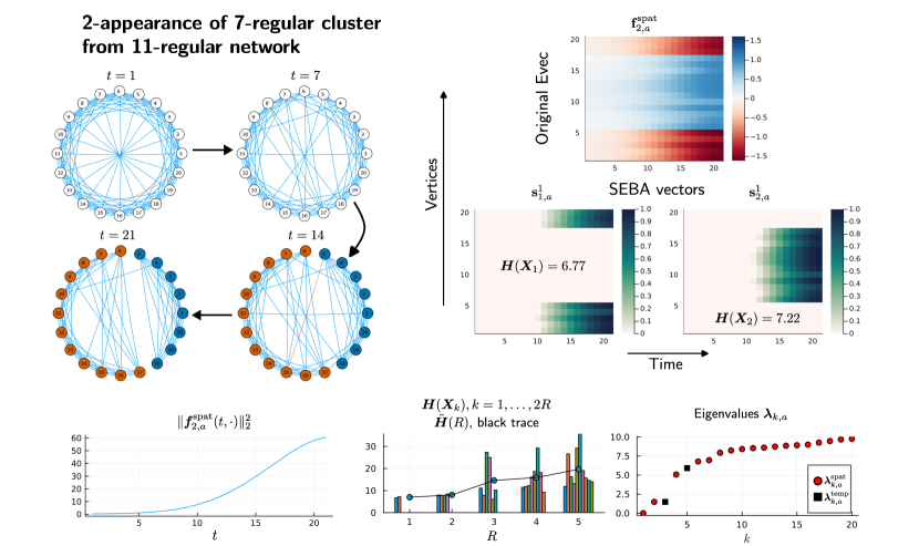
Figure 4: Spectral partitioning of spacetime graphs with the inflated dynamic Laplacian to discover the 2-appearance of clusters discussed in in Sec. 5.1. (Upper left) Multiple time slices of the spacetime graph. The vertices are coloured according to assignments from individual SEBA vectors computed using the unnormalised Laplacian $\bm{\mathrm{L}}^{(a)}$. Red edges indicate edges at time $t$ that are removed at time $t+1$. (Upper right) Cluster detection using spectral partitioning. Using $R=1$, the spatial eigenvector $\bm{\mathrm{f}}^{\rm spat}_{2,a}$ of the inflated dynamic Laplacian $\smash{\bm{\mathrm{L}}^{(a)}}$ and the corresponding two SEBA vectors $\smash{\bm{\mathrm{s}}^{1}_{1,a},\bm{\mathrm{s}}^{1}_{2,a}}$, supporting clusters $\bm{X}_{1},\bm{X}_{2}$ respectively, with Cheeger values computed using (18). The complete lack of support of $\bm{\mathrm{s}}^{1}_{1,a},\bm{\mathrm{s}}^{1}_{2,a}$ during times earlier than $t=10$ indicates the unclustered spacetime nodes $\bm{\Omega}$. (Lower left) Plot of $\smash{\|\bm{\mathrm{f}}_{2,a}^{\rm spat}(t,\cdot)\|_{2}^{2}}$ versus $t$, which demonstrates growing confidence in partitioning as time increases. Also shown are (Lower middle) plots of the cut function $\bm{H}(\bm{X}_{k})$ for $k=1\dots 2R$, vs $R$, where $\bm{X}_{k}$ is the support of SEBA vector $\bm{\mathrm{s}}_{k,a}^{R}$ and the (Lower right) eigenvalues $\bm{\lambda}_{k,a}$, sorted by spatial (red circles) and temporal (black squares).

The mean Cheeger ratios $\smash{\tilde{\bm{H}}(R)}$ in Fig. 4 (lower center) remain low for $R=1$ and $R=2$. We therefore fix $R=1$ because this is a good choice in terms of both spectral gap and low cut values. Algorithm 1 returns the first nontrivial spatial eigenvector ${\bm{\mathrm{f}}}^{\rm spat}_{2,a}$ of ${\bm{\mathrm{L}}}^{(a)}$, the corresponding SEBA vectors $\smash{{\bm{\mathrm{s}}}^{1}_{1,a},{\bm{\mathrm{s}}}^{1}_{2,a}}$, and the associated clusters $\bm{X}_{1},\bm{X}_{2}$ and unclustered set $\bm{\Omega}$.

For comparison, we also perform cluster detection using the Leiden algorithm [TWvE19]. The algorithm is an iterative aggregation-based cluster-identification procedure that maximises modularity. We stop the algorithm when there is no further increase in modularity. The algorithm is applied to our network in two ways: slice-by-slice and on the whole graph. In the slice-by-slice case, Leiden (the shorthand name used for the Leiden algorithm) is used to discover clusters on every time slice. We then use a matching technique to connect the various spatial clusters into spacetime clusters, see Appendix F. Ad hoc matching techniques have been used before to link individual spatial clusters in time, see [MOR20] for example. Our approach solves a maximum weight edge cover problem to maximise intercluster weights and optimise temporal matching. The results are shown in Fig. 5 (upper row). We also report the values of the cut function $\bm{H}(\bm{X}_{k})$ for each of the clusters obtained from our spectral partitioning algorithm and Leiden.

5.1.3 Discussion of clustering

In Fig. 4 we observe that the first nontrivial spatial eigenvector ${\bm{\mathrm{f}}}^{\rm spat}_{2,a}$ gives a clear spacetime partition that separates the two sets of spatial vertices $\{1,\ldots,5,18,\ldots,20\}$ (red, negative values) and $\{6,\ldots,17\}$ (blue, positive values) through time. This can be visualised by the increase in $\|{\bm{\mathrm{f}}}^{\rm spat}_{2,a}(t,\cdot)\|$ as $s$ increases (see Fig. 4, lower left). The SEBA vectors clearly separate the appearing clusters after around $t=10$ and have zero support in the early time interval $t=1$ to $t=9$ where the graphs on individual time slices are close to regular.

We compare these results with those obtained using the Leiden algorithm in Fig. 5 (upper panel). The slice-by-slice Leiden computations show that the network is partitioned into three clusters while the network is still near-regular ($t=1$ to $t=7$). However at later times, the correct two clusters are recovered. Nevertheless, the value $\max_{1\leq k\leq 3}\bm{H}(\bm{X}_{k})=\bm{H}(\bm{X}_{3})=29.7$ for the Leiden slice-by-slice case is very large compared to that of the spectral partitioning method, where $\max_{1\leq k\leq 3}\bm{H}(\bm{X}_{k})=\bm{H}(\bm{X}_{2})=7.22$ (with the identification $\bm{X}_{3}=\bm{\Omega}$). Thus our approach provides a better balanced cut than the Leiden algorithm.

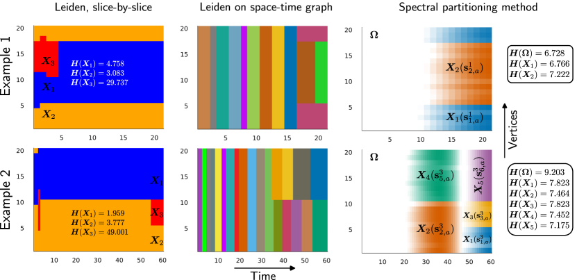
Figure 5: Comparing spectral partitioning with modularity maximisation using the Leiden algorithm [TWvE19] for the two example networks. Leiden is performed for two scenarios of the spacetime graph: slice-by-slice (left column) and on the whole spacetime graph (middle column). Cheeger values are computed using (18), and shown for the slice-by-slice case only. Also shown (right column) are the individual clusters obtained from the spectral partitioning Algorithm 1 presented in Fig. 4 and Fig. 6. In the first example (upper right), SEBA vectors $\bm{\mathrm{s}}^{1}_{j,a}$ for $j=1,2$ and the non-empty unclustered set $\Omega$ are used to create a 3-partition of the network. In the second example (lower right), SEBA vectors $\bm{\mathrm{s}}^{3}_{j,a}$ for $j=1,2,3,5,6$ and the non-empty unclustered set $\bm{\Omega}$ are used to create a 6-partition of the network.

Using Leiden on the spacetime graph (Fig. 5, upper middle) yields a spatial separation of clusters only at the very late times $t=17$ to $t=20$, where the appropriate two clusters $\{1,\ldots,5,18,\ldots,20\}$ and $\{6,\ldots,17\}$ are recovered. At times prior to $t=17$, spurious partitioning of many time slices into its own cluster renders these results unusable. The respective Cheeger function values $\bm{H}(\bm{X}_{k})$ of such clusters are $2a^{2}\approx 133.15$, which is significantly larger than the values for clusters obtained using our spacetime partitioning method.

5.2 Example 2: Appearance of two clusters followed by splitting

We extend the previous example by allowing one of the appearing clusters to split into two clusters. Depending on the cluster labelling, this could be described as either a 2-splitting, or a 2-disappearance, followed by a 1-appearance and a 2-appearance. We expect to resolve the emerging cluster and its splitting using the eigenvectors of the corresponding inflated dynamic Laplacian. The results from the following example are presented in Fig. 6.

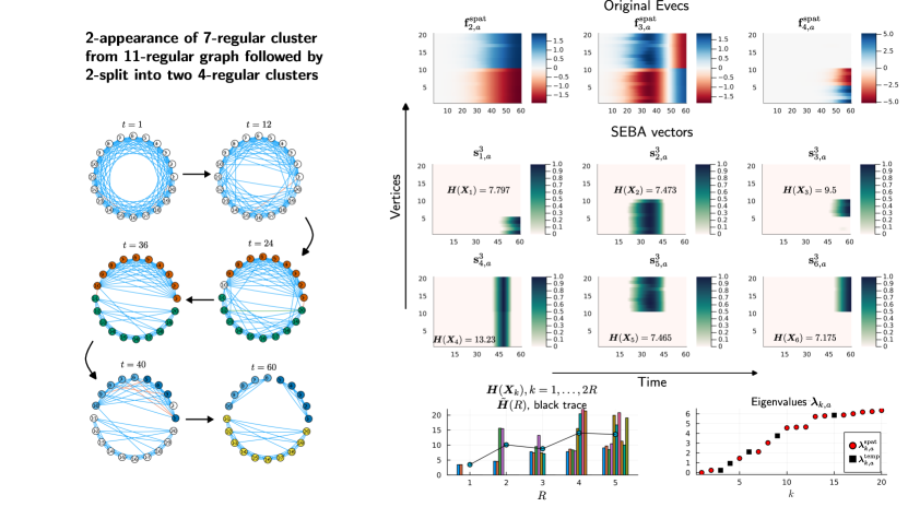
Figure 6: Spectral partitioning of spacetime graphs with the inflated dynamic Laplacian $\bm{\mathrm{L}}^{(a)}$ to discover a 2-appearance followed by a 2-disappearance, immediately followed by a 1-appearance and a 2-appearance. With cluster relabelling, one could more simply say we have a 2-appearance followed by a 2-split. (Left) Multiple time slices of the spacetime graph. The vertices are coloured according to assignments from individual SEBA vectors computed. Red edges indicate edges at time $t$ that are removed at time $t+1$. (Right?) Cluster detection using spectral partitioning. (Upper right) First three spatial eigenvectors $\smash{{\bm{\mathrm{f}}}^{\rm spat}_{(2,3,4),a}}$ of the inflated dynamic Laplacian $\bm{\mathrm{L}}^{(a)}$. (Center right?) Six SEBA vectors ${\bm{\mathrm{s}}}^{3}_{i,a}$ for $i=1,\ldots,6$ computed using the three spatial eigenvectors above with Cheeger values computed using (18). Also shown (Lower right) are plots of the Cheeger values $\bm{H}(\bm{X}_{k})$ for $k=1,\dots,6$, where $\bm{X}_{k}$ is the support of SEBA vector ${\bm{\mathrm{s}}}_{k,a}^{3}$ and the eigenvalues ${\bm{\lambda}}_{k,a}$, sorted by spatial (red circles) and temporal (black squares).

5.2.1 Graph construction

The graph is constructed with $N=20$ and $T=60$. At $t=1$, the graph is $11$-regular as in the previous example and slowly transitions to a graph at $t=36$ that contains two highly intraconnected clusters linked by a single edge. One of these clusters then slowly splits into two separate clusters at $t=60$. The graphs are represented by adjacency matrices $\{\mathrm{W}^{\rm spat}_{t}\}$, $t=1,\dots,60$, such that $\mathrm{[}W^{\rm spat}_{t}]_{ij}\in\{0,1\}$, $\forall i,j,t$. A few snapshots of the network are shown in Fig. 6 (left panel).

5.2.2 Cluster detection

We use Algorithm 1 to compute the individual clusters. Using Step 3 of Algorithm 1 we obtain the critical value $a=9.27364$ which is fixed for the rest of the computations. The parameter $R$ tells one how many of the first $R$ nontrivial spatial eigenvectors $\bm{\mathrm{f}}^{\rm spat}_{k,a}$, $k=2,\ldots,R+1$ should be used for spectral partitioning. At $R=1$ there is a significant spectral gap between ${\bm{\lambda}}^{\rm spat}_{2,a}$ and ${\bm{\lambda}}^{\rm spat}_{3,a}$. There is also a large gap at $R=3$, between ${\bm{\lambda}}^{\rm spat}_{4,a}$ and ${\bm{\lambda}}^{\rm spat}_{5,a}$, see Fig. 6 (lower right). The mean Cheeger ratios $\tilde{\bm{H}}(R)$ plotted in Fig. 6 (lower right, black trace) shows a global minimum at $R=1$ and a local minimum at $R=3$. Therefore, reasonable choices of $R$ would be $R=1$ and $R=3$. The former choice would reveal the 2-splitting we have already discussed in Example 1. We therefore set $R=3$, which provides further information, and will identify additional splittings. Algorithm 1 returns the first three nontrivial spatial eigenvectors ${\bm{\mathrm{f}}}^{\rm spat}_{2,a}$ ${\bm{\mathrm{f}}}^{\rm spat}_{3,a}$, and ${\bm{\mathrm{f}}}^{\rm spat}_{4,a}$ of ${\bm{\mathrm{L}}}^{(a)}$, the corresponding SEBA vectors $\smash{{\bm{\mathrm{s}}}^{3}_{j,a}},j=1,\ldots,6$, and the associated clusters $\bm{X}_{j}$, $j=1,\ldots,6$ and unclustered set $\bm{\Omega}$.

Similar to the previous example we also perform computations using the Leiden algorithm. We compare the results of the spectral partitioning method with those obtained using Leiden in Fig. 5 (lower).

5.2.3 Discussion of clustering

In Fig. 6 (right panel) we show the vectors ${\bm{\mathrm{f}}}^{\rm spat}_{2,a}$ and ${\bm{\mathrm{f}}}^{\rm spat}_{3,a}$ that capture the slowly emerging two clusters at $t=36$ and their persistence until $t=60$. These clusters are represented by vertices $\{1,\dots,10\}$ and $\{11,\ldots,20\}$ respectively. The vector ${\bm{\mathrm{f}}}^{\rm spat}_{4,a}$ resolves the slow splitting of the cluster $\{1,\ldots,10\}$ into the clusters $\{1,\ldots,5\}$ and $\{6,\ldots,10\}$. The corresponding SEBA vectors ${\bm{\mathrm{s}}}^{3}_{j,a}$ successfully capture the $5$ individual clusters except for ${\bm{\mathrm{s}}}^{3}_{4,a}$, which is a spacetime cluster that contains all vertices for the time that it exists. The SEBA vector ${\bm{\mathrm{s}}}^{3}_{4,a}$ is identified as spurious by step 7 of Algorithm 1 and also corresponds to a high Cheeger value $\bm{H}(\bm{X}_{4})=13.23$ compared to the other clusters. We therefore discard it to obtain a $K$-partition with $K=6$ (5 SEBA vectors and the unclustered set $\Omega$). By post-processing the cluster assignment with our optimal matching algorithm described in Appendix F.1, one could relabel $\bm{X}_{5}$ as $\bm{X}_{4}$ and $\bm{X}_{3}$ as $\bm{X}_{2}$, to reduce $K$ from 6 to 3 and further reduce the Cheeger values.

In Fig. 5 (lower panel) we show the slice-by-slice and full spacetime graph computations using the Leiden algorithm. The slice-by-slice clustering is not completely satisfactory in how it captures the emergence of two clusters followed by the splitting. The value $\max_{1\leq k\leq 3}\bm{H}(\bm{X}_{k})=\bm{H}(\bm{X}_{3})=49.001$ is large compared to the clusters detected using the spectral partitioning algorithm ($\max_{1\leq k\leq 6}\bm{H}(\bm{X}_{k})=\bm{H}(\bm{\Omega})=9.203$, with the identification $\bm{X}_{6}=\bm{\Omega}$). Note that from Proposition 2, given a good candidate partition $\bm{\mathfrak{X}}=\{\bm{X}_{1},\ldots,\bm{X}_{K}\}$ we should get higher values of $\max_{k}\bm{H}(\bm{X}_{k})$ for a 6-partition compared to a 3-partition. Yet, we see that the spectral partitioning algorithm even outperforms Leiden, despite the former providing a $6$-partition and the latter providing only a $3$-partition.

6 Networks with vertices that appear and disappear in time

In this section we use spectral partitioning on networks where vertices appear and disappear as time passes. This requires using a non-multiplex form of a spacetime graph. We begin with a demonstration of our spatiotemporal spectral clustering using a toy model that contains vertices that appear and disappear. We then consider a real-world network of voting similarities between senators of the US Senate between the years 1987 and 2009. This network was considered in [WPF⁺09, MRM⁺10] to analyse polarisation in US politics. Our spatiotemporal spectral partitioning technique reveals the onset and magnitude of polarisation as time passes, which to our knowledge has not been shown before.

6.1 A non-multiplex framework

To work with vertices that appear and disappear in time, we propose a non-multiplex framework. Consider a network with $T$ time slices with each slice having a maximum of $N$ vertices that may appear or disappear in time. The network configuration is shown in Fig. 7 (left). Vertices are split into two types: present (red/blue) and absent (white). The entire collection of present spacetime vertices is denoted by $\bm{V}$ with cardinality $N^{\prime}>0$. We create a superset of spatial vertices

$$\hat{V}:=\bigcup_{t=1}^{T}\{x:(t,x)\in\bm{V}\},$$

and identify the vertices in $\hat{V}$ with integers $1,\ldots,N$. For each $t$, denote the vertices on the $t$-th time fibre by $V_{t}:=\{x:(t,x)\in\bm{V}\}\subset\{1,\ldots,N\}$, each with cardinality $N_{t}\leq N$. Thus, $\sum_{t=1}^{T}N_{t}=N^{\prime}$. For each $t=1,\dots,T$, the spatial network on $V_{t}$ is given by a spatial adjacency $\mathrm{W}^{\rm spat}_{t}\in\mathbb{R}^{N_{t}\times N_{t}}$. Note that here $N^{\prime}<TN$ while in the multiplex case $N^{\prime}=TN$. The non-multiplex spacetime weights $\bm{\mathcal{W}}^{(a)}$ on $\bm{V}$ are then defined as

$$\bm{\mathcal{W}}^{(a)}_{(t,x),(t,y)}=\mathrm{[}W^{\rm spat}_{t}]_{xy} \textnormal{ if }x,y\in V_{t}\,,$$ (44)

$$\bm{\mathcal{W}}^{(a)}_{(t,x),(t+1,x)}=a^{2} \textnormal{ if }(t,x),(t+1,x)\in\bm{V}.$$

The resulting spacetime graph is no longer multiplex as not all vertices at a time slice are connected to their neighbours in the adjacent time slices. This is illustrated in Fig. 7 (left).

The matrix forms are defined as follows. First we define the lexicographic ordering $i$ such that

$$\bm{i} :(t,x)\mapsto\sum_{s=1}^{t-1}N_{s}+x,$$ (45)

$$\bm{i} (\bm{V})=\left\{1,\dots,N_{1},N_{1}+1,\dots,\textstyle\sum_{s=1}^{t}N_{s}-1,\sum_{s=1}^{t}N_{s}\right\}.$$

The matrix $\bm{\mathrm{W}}^{(a)}$ is assembled using the above ordering in the rows and columns, similar to (33):

$$\bm{\mathrm{W}}^{(a)}=\begin{bmatrix}\bm{\mathcal{W}}^{(a)}_{(1,1),(1,1)}&\dots&\bm{\mathcal{W}}^{(a)}_{(1,1),(T,N_{t})}\\ \vdots&&\vdots\\ \bm{\mathcal{W}}^{(a)}_{(T,N_{t}),(1,1)}&\dots&\bm{\mathcal{W}}^{(a)}_{(T,N_{t}),(T,N_{t})}\end{bmatrix}.$$ (46)

The inflated dynamic Laplacian matrix $\bm{\mathrm{L}}^{(a)}$ is constructed using (40). We do not split the matrices $\bm{\mathrm{L}}^{(a)}$ and $\bm{\mathrm{W}}^{(a)}$ into its temporal and spatial components, as the simple occupation structure from Fig. 2 is lost in the non-multiplex setting.

Choosing $a$ for the non-multiplex framework.

As we do not have a clear distinction between spatial and temporal eigenvectors of the corresponding inflated dynamic Laplacian $\bm{\mathrm{L}}^{(a)}$, we cannot fix $a$ as in step 3 of Algorithm 1. We use a new heuristic to determine $a$. In Algorithm 1 we balance spatial and temporal diffusion by finding $a$ such that ${\bm{\lambda}}_{2,a}^{\rm spat}={\bm{\lambda}}_{2,a}^{\rm temp}$. We observe numerically that in the multiplex case, this heuristic yields an $a$ that is identical to the $a$ obtained by balancing the spatial and temporal contributions of the Rayleigh quotient corresponding to the spatial eigenvalue. In other words we conjecture that

$$\bm{\lambda}_{2,a}^{\rm spat}=\bm{\lambda}_{2,a}^{\rm temp}\iff\langle\bm{\mathrm{L}}^{\rm spat}\bm{\mathrm{f}}^{\rm spat}_{2,a},\bm{\mathrm{f}}^{\rm spat}_{2,a}\rangle=a^{2}\langle\bm{\mathrm{L}}^{\rm temp}\bm{\mathrm{f}}^{\rm spat}_{2,a},\bm{\mathrm{f}}^{\rm spat}_{2,a}\rangle.$$ (47)

In the multiplex case, there is no notion of $\bm{\lambda}_{2,a}^{\rm temp}$, and we cannot use the left-hand equality in (47) to select $a$. Instead, we compute the value of $a$ for which $\langle\bm{\mathrm{L}}^{\rm spat}\bm{\mathrm{f}}_{2,a},\bm{\mathrm{f}}_{2,a}\rangle=a^{2}\langle\bm{\mathrm{L}}^{\rm temp}\bm{\mathrm{f}}_{2,a},\bm{\mathrm{f}}_{2,a}\rangle$, where $\bm{\mathrm{f}}_{2,a}$ is the second eigenvector of $\bm{\mathrm{L}}^{(a)}$.

Input : Diffusion constant $a$, non-multiplex inflated dynamic Laplacian $\bm{\mathrm{L}}^{(a)}\in\mathbb{R}^{N^{\prime}\times N^{\prime}}$.

Output : Eigenvectors $\{\bm{\mathrm{f}}_{k,a}\}_{k=k_{1},k_{2},\ldots,k_{R}}$ representing “spatial” eigenvectors of the non-multiplex network.

1 Compute eigenvectors $\bm{\mathrm{f}}_{k,a}\in\mathbb{R}^{N^{\prime}}$, $k=1,\ldots,N^{\prime}$. Set $\tilde{\mathrm{f}}_{j}^{\rm temp}$ to be the $j$-th eigenvector of the Laplacian $\mathrm{L}^{\prime}$. Set $\tilde{\bm{\mathrm{f}}}_{j}^{\rm temp}=\tilde{\mathrm{f}}_{j}^{\rm temp}\otimes\mathbbm{1}_{N}\in\mathbb{R}^{TN}$, $j=1,\ldots,T$ using (37) with $N$ vertices and $T$ time slices;

2 For each $k$ compute the inner product $\max_{j=1,\ldots,T}|\langle\mathcal{I}(\bm{\mathrm{f}}_{k,a}),\tilde{\bm{\mathrm{f}}}_{j}^{\rm temp}\rangle|$, where $\mathcal{I}(\cdot):\mathbb{R}^{N^{\prime}}\to\mathbb{R}^{TN}$ is the natural inclusion of present vertices;

Declare $R$ vectors (namely $\{\bm{\mathrm{f}}_{k,a}\}_{k=k_{1},k_{2}\ldots,k_{R}}$) with low inner product values in the previous step as “spatial”.

Algorithm 2 Algorithm to find spatial eigenvectors for the non-multiplex graph Laplacians.

With Algorithm 2, we construct a version of Algorithm 1 that handles the non-multiplex situation.

Input : Superset of of vertices $N$, number of time slices $T$, graph $\bm{G}$ represented by collection of spatial adjacencies $\{\mathrm{W}^{\rm spat}_{t}\}_{t=1,\dots,T}$, $\mathrm{W}^{\rm spat}_{t}\in\mathbb{R}^{N_{t}\times N_{t}}$, $\sum_{t}N_{t}=:N^{\prime}<TN$.

Output : $K$-packing $\{\bm{X}_{n_{1}},\ldots,\bm{X}_{n_{K}}\}$

1 Construct $\bm{\mathrm{W}}^{(a)}$ as described in Sec. 6.1 and consequently the corresponding $\bm{\mathrm{L}}^{(a)}$ using (40);

2 Identify spatial eigenvalues using Algorithm 2 and compute $a=a_{c}$ such that temporal and spatial diffusion is balanced using the heuristic explained in Sec. 6.1;

3 Compute $(\bm{\lambda}_{k,a},\bm{\mathrm{f}}_{k,a})$, the $k$-th eigenpair of $\bm{\mathrm{L}}^{(a)}$ for $k=2,\ldots,R+1$. Select a suitable value for $R$ as described in step 4 of Algorithm 1;

4

5Isolate spacetime packing elements: Apply the SEBA algorithm [FRS19] to the collection $\{\bm{\mathrm{f}}_{k_{1},a},\dots,\bm{\mathrm{f}}_{k_{R},a}\}$. The output SEBA vectors are denoted $\{\bm{\mathrm{s}}^{R}_{j,a}\}_{j=1,\dots,R}$;

6 Identify spurious SEBA vectors: If the $j^{th}$ SEBA vector is approximately constant on each index block corresponding to a single time fibre, i.e. if $[\bm{\mathrm{s}}^{R}_{j,a}]_{z}\approx C_{j,t}$ for $z=\bm{i}(t,x)$, $1\leq x\leq N$, $1\leq t\leq T$, where $\bm{i}$ is defined in (45);

Define packing elements: Let $\{{n_{1}},\ldots,{n_{K}}\}$, $K\leq R$ denote indices of the non-spurious SEBA vectors. Define $\bm{X}_{n_{j}}=\{(t,x)\,:\,[\bm{\mathrm{s}}^{R}_{n_{j},a}]_{z}>0,z=\bm{i}(t,x)\}$ for each $j=1,\ldots,K$. If a single spacetime vertex $(t,x)$ belongs to two or more $\bm{X}_{n_{j}}$, assign it only to the $\bm{X}_{n_{j}}$ with the largest $[\bm{\mathrm{s}}^{R}_{n_{j},a}]_{z}$ value. One may augment the packing with the unclustered set $\bm{\Omega}=\{(t,x)\,:\,\smash{[\bm{\mathrm{s}}^{R}_{n_{j},a}]_{z}}=0,z=\bm{i}(t,x)\}$ to obtain a $K+1$ partition.

Algorithm 3 Spectral partitioning in the non-multiplex case.

6.2 A toy model with appearing/disappearing vertices

We consider a non-multiplex network with spacetime nodes $\bm{V}$ shown as blue or red in Fig. 7 (right).

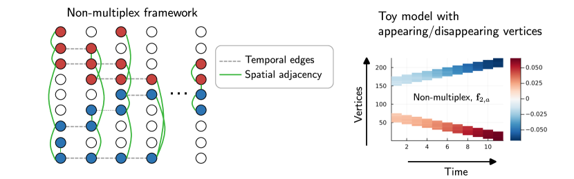
Figure 7: Spectral partitioning on networks with vertices that appear/disappear over time. (Left) Non-multiplex framework, where vertices are connected to their time-analogues only if the vertex is active (red/blue) in the next time slice. (Right) Spectral partitioning on a toy network. A network of 225 vertices and 11 time slices is constructed such that at each time, 5 vertices are exchanged between each cluster and the inactive vertices. The inter-cluster edge weights are set to $i/T$ for $i=1,\dots,T$. The eigenvector ${\bm{\mathrm{f}}}_{2,a}$ corresponding to the unnormalised Laplacian ${\bm{\mathcal{L}}}^{(a)}$ is shown.

The cardinality of $\hat{V}$ is 225 and there are $T=11$ time slices. For each time slice $t$, we assign node weights that clearly define two $16$-regular clusters: $\bm{C}_{1}:=\{51-5(t-1),\ldots,75-5(t-1)\}$ and $\bm{C}_{2}:=\{151-5(t-1),\dots,175-5(t-1)\}$. As $t$ increments to $t+1$, each cluster retains $20$ vertices from the old clusters, loses $5$ vertices that become absent, and gains $5$ newly appearing vertices. The intercluster edges are randomly assigned such that a maximum of $20$% of the total edges assigned to any present vertex is an intercluster edge. The weights $[W^{\rm spat}_{t}]_{x,y}$ for a pair of present vertices $x$ and $y$ at slice $t$ such that

$$[W^{\rm spat}_{t}]_{x,y}=\begin{cases}1,&\mbox{if $x,y\in\bm{C}_{1}$ or $x,y\in\bm{C}_{2}$,}\\ 1/t,&\mbox{otherwise.}\\ \end{cases}$$ (48)

We now implement the non-multiplex framework to formulate the corresponding new adjacency matrix $\bm{\mathrm{W}}^{(a)}$.

For our spectral clustering we first fix $a=5.5844$ using step 2 in Algorithm 3 (implementing the heuristic introduced at the end of Sec. 6.1). Note that the value of $\bm{\lambda}_{2,a}=\bm{\lambda}_{2,a}^{\rm spat}=0.29955$. We use the new Algorithm 3 to perform spectral partitioning. Using step 2 in the Algorithm 2, we find inner products $\smash{\max_{j}|\langle\mathcal{I}(\bm{\mathrm{f}}_{2,a}),\tilde{\bm{\mathrm{f}}}^{\rm temp}_{j}\rangle|=0.00516}$ and $\smash{\max_{j}|\langle\mathcal{I}(\bm{\mathrm{f}}_{3,a}),\tilde{\bm{\mathrm{f}}}^{\rm temp}_{j}\rangle|=0.47044}$ and conclude that $\bm{\mathrm{f}}_{2,a}$ corresponds to the first nontrivial spatial eigenvector. Note that the inner product $\smash{\langle\mathcal{I}(\bm{\mathrm{f}}_{k,a}),\tilde{\bm{\mathrm{f}}}_{j}^{\rm temp}\rangle}$ is equivalent to computing correlation coefficients $\rho(\mathcal{I}(\bm{\mathrm{f}}_{k,a}),\smash{\tilde{\bm{\mathrm{f}}}_{j}^{\rm temp}})\in[-1,1]$ for mean-zero and $\ell_{2}$-normalised vectors.

The first five nontrivial spatial eigenvalues are $\bm{\lambda}_{2,a}=0.3029,\bm{\lambda}_{4,a}=1.3638,\bm{\lambda}_{6,a}=4.1389,\bm{\lambda}_{8,a}=7.7838$ and $\bm{\lambda}_{10,a}=10.0706$. As there is no unambiguous spectral gap, we look at mean Cheeger values $\tilde{\bm{H}}(R)$. For $R=1,2,3$ we have the corresponding values $\tilde{\bm{H}}(R)=0.5969,2.2080,4.8186$. Consequently, we choose $R=1$ – as larger $R$ will create significantly worse Cheeger values – and use $\bm{\mathrm{f}}_{2,a}$ to perform spectral clustering. In Fig. 7 (right), we show the plot of the second eigenvector $\bm{\mathrm{f}}_{2,a}$. The two persistent clusters are recovered. Moreover, the magnitude of $\bm{\mathrm{f}}_{2,a}$ increases with time (represented by darker colours as we move to the right) as the clustering becomes stronger due to the intercluster spatial edges becoming weaker as time increases. This is a vital observation for the following section when we discuss the network of US senators.

6.3 A network of US senators and states to analyse polarisation

In this section we use the dense and non-multiplex approaches on a network of voting similarities in the US Senate between the years 1987 and 2009. The network represents senators as vertices and has edges weighted by a factor in the range $[0,1]$, which describes the voting similarity between two senators (fraction of identical votes). A higher value indicates that the pair of senators had a large share of common votes on the various bills that they legislated on in the Senate. The network is constructed using details on senators and their votes from www.voteview.com. More details on the construction of the network can be found in [WPF⁺09].

6.3.1 A network of senators

Consider a sequence of weight matrices $\{\mathrm{W}^{\rm spat}_{t}\}_{t=1,\dots,T}$, $\mathrm{W}^{\rm spat}_{t}\in\mathbb{R}^{N_{t}\times N_{t}}$ with $N=225$ vertices each and $T=11$ time slices. Each vertex in $V^{\prime}$ represents a unique senator that served between the years 1987 and 2009. This corresponds to the congresses numbered in the interval 100–110. The weights $\mathrm{W}^{\rm spat}_{t}$ on the edges between any two vertices describe the voting similarity between the two corresponding senators in congress $99+t$. The weights $W^{\rm spat}_{t}$ are defined by

$$[\mathrm{W}^{\rm spat}_{t}]_{x,y}=\frac{1}{|\Omega_{xyt}|}\sum_{i\in\Omega_{xyt}}\delta_{b_{ixt},b_{iyt}},$$ (49)

where $\Omega_{xyt}$ is the set of bills voted on by both senators $x$ and $y$ at congress $99+t$ and $\delta$ is the Kronecker delta function such that $\delta_{ij}=1\iff i=j$, $0$ otherwise; thus, the weights $\smash{[\mathrm{W}^{\rm spat}_{t}]_{x,y}\in[0,1]}$. The expression $b_{ixt}$ represents the vote of a senator $x$ for bill $i$ in congress $99+t$; cf. [WPF⁺09]. The vote is assigned a value of $1$ if voted “yes” and assigned $-1$ if voted “no”. The vote is set to $0$ in case of abstention. Next, we construct $\bm{\mathrm{W}}^{(a)}$ using the non-multiplex framework as discussed previously and formulate the unnormalised inflated dynamic Laplacian $\bm{\mathrm{L}}^{(a)}$. We then use the spectral partitioning Algorithm 3 to detect communities in this network.

Clustering using ${\bm{\mathrm{f}}}_{3,a}$ from the non-multiplex senator network.

In Algorithm 2, step 2, we compute the inner products $\max_{j}|\langle\mathcal{I}(\bm{\mathrm{f}}_{2,a}),\smash{\tilde{\bm{\mathrm{f}}}^{\rm temp}_{j}}\rangle|=0.63426$ and $\max_{j}|\langle\mathcal{I}(\bm{\mathrm{f}}_{3,a}),\tilde{\bm{\mathrm{f}}}^{\rm temp}_{j}\rangle|=0.03537$ and thus identify $\bm{\mathrm{f}}_{2,a}$ and $\bm{\mathrm{f}}_{3,a}$ as temporal and spatial eigenvectors respectively. Using Algorithm 3, step 2 we find the value $a=21.51392$ as the critical $a$ for the senator network. Next, in step 3 of Algorithm 3, we compute several leading eigenvectors $\bm{\mathrm{f}}_{k,a}$ of $\bm{\mathrm{L}}^{(a)}$, displayed in Fig. 8 (second column, upper panel). The first five nontrivial spatial eigenvalues are $\bm{\lambda}_{3,a}=33.988,\bm{\lambda}_{7,a}=49.4765,\bm{\lambda}_{9,a}=50.1136,\bm{\lambda}_{10,a}=50.4866$ and $\bm{\lambda}_{11,a}=50.9579$. As there is significant spectral gap between $\bm{\lambda}_{3,a}$ and $\bm{\lambda}_{7,a}$, we choose $R=1$, and use $\bm{\mathrm{f}}_{3,a}$ to perform spectral clustering. The eigenvectors shown in Fig. 8 (first column, centre panel) have a particular senator ordering for convenience. The senators are sorted by their respective temporal means computed from $\bm{\mathrm{f}}_{3,a}$ (i.e. sorted according to average values along horizontal rows in the image). A clear 2-partition is visible, which coincides with the respective party membership of the associated senators, see Fig. 8 (first column, lower panel).

There are two main conclusions one can draw from the plot of the eigenvector $\bm{\mathrm{f}}_{3,a}$ in Fig. 8 (centre left). First, the partitioning of a network based on voting similarities coincides with the partition arising from party memberships shown in Fig. 8 (lower left), which implies that senators are most likely to vote along party lines. Second, the norm of $\bm{\mathrm{f}}_{3,a}$ restricted to the 11 individual congresses increases as time passes. This is seen by a darkening of colours from left to right in Fig. 8 (centre left), and corresponds to a higher confidence of partitioning the individual time slices. This can be explained by the inter-cluster edge weights, which decrease as time passes, similar to the toy model from the previous section. In this way we demonstrate growing polarisation between the years 1987 and 2009 in US politics.

6.3.2 A network of states

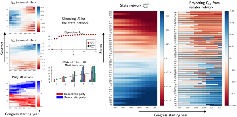
Figure 8: Polarisation in voting patterns of US senators over 11 congresses (numbered 100-110) between the years 1987–2009. First column: Spectral partitioning of the network of senators constructed using the non-multiplex approach. Eigenvectors $\bm{\mathrm{f}}_{2,a}$ (upper) and $\bm{\mathrm{f}}_{3,a}$ (centre) corresponding to the unnormalised Laplacian $\bm{\mathrm{L}}^{(a)}$ are shown. The vertices in the senator network are ordered according to the temporal means of the spatial fibres $\bm{\mathrm{f}}_{k,a}(x,\cdot)$. Also shown are party affiliations corresponding to senators over time (lower): Democrat (blue) and Republican (red). Second column: Plots of eigenvalues $\bm{\lambda}_{k,a}$ (upper) and Cheeger values $\bm{H}(\bm{X}_{k})$ and $\tilde{\bm{H}}(R)$ for various values of $R$ (lower) for the state network. Third column: Spectral partitioning of the network of states discussed in Section 6.3.2. The first spatial eigenvector $\smash{\bm{\mathrm{f}}^{\rm spat}_{2,a}}$ corresponding to the unnormalised Laplacian $\bm{\mathrm{L}}^{(a)}$ is shown. Fourth column: To compare with the third column, we display $\bm{\mathrm{f}}_{3,a}$ from the non-multiplex senator network (first column, centre panel) now re-ordered by state affiliation. There are two senators for each state, which are demarcated between different states by black lines.

We now construct a network with US states as space vertices, and spatial edges between two spacetime vertices at time $t$ weighted by the voting similarity of the two corresponding states over the single congress period $99+t$. From 1987–2009, the US had 50 states, so this network is of multiplex type. The network of states is represented by a sequence of adjacency matrices $\{\mathrm{W}^{\rm spat}_{t}\}_{t=1,\dots,T}$, $\mathrm{W}^{\rm spat}_{t}\in\mathbb{R}^{N\times N}$ with $N=50$ vertices per time slice and $T=11$ time slices. We first define the “aggregate vote” $b^{\rm state}_{ixt}$ made by a state $x$ on bill $i$ in congress $99+t$, using the individual senator votes $b_{i\sigma t}$ as follows (bill $i$, senator $\sigma$, time $t$),

$$b^{\rm state}_{ixt}=\sum_{\sigma\in x}b_{i\sigma t}.$$ (50)

The weights $[\mathrm{W}^{\rm spat}_{t}]_{x,y}$ are then given by

$$[\mathrm{W}^{\rm spat}_{t}]_{x,y}=\frac{1}{|\Omega^{\rm state}_{xyt}|}\sum_{i\in\Omega^{\rm state}_{xyt}}\delta_{b_{ixt}^{\rm state},b_{iyt}^{\rm state}},$$ (51)

where $\Omega_{xyt}^{\rm state}$ is the set of votes jointly voted on by senators $\sigma$ belonging to states $x$ and $y$ in congress $99+t$, and $\delta$ is the Kronecker delta as before. Consequently, $[\mathrm{W}^{\rm spat}_{t}]_{x,y}\in[0,1]$. The sequence $\{\mathrm{W}^{\rm spat}_{t}\}_{t=1,\dots,T}$ is then used for spectral partitioning using Algorithm 1 to detect clusters.

As the network is of multiplex type, we can directly use Algorithm 1, e.g. step 3 to compute $a=8.88452$ and construct $\bm{\mathrm{L}}^{(a)}$, and step 4 to determine $R$, as discussed in Sec. 4.2. Regarding the choice of $R$, in Fig. 8 (second column, upper panel) we see that the main nontrivial gap is between the 2nd and 3rd spatial eigenvalues, suggesting $R=1$. The lower panel of the second column in Fig. 8 shows the plot of the average Cheeger value $\tilde{\bm{H}}(R)$. The average Cheeger values increase consistently with increasing $R$ and there does not seem to be a possibility to form more than two clusters with low Cheeger value. For this reason, and the above spectral gap considerations, we fix $R=1$.

In Fig. 8 (third column) we plot the first nontrivial spatial eigenvector $\bm{\mathrm{f}}^{\rm spat}_{2,a}$ (the second spatial eigenvector) of $\bm{\mathrm{L}}^{(a)}$ computed from the state network. The vertices are labelled with their respective state abbreviations and sorted according to the temporal average of the displayed eigenvector (i.e. sorted according to average values along horizontal rows in the image). We observe a clear 2-partition in the state network (upper vs lower states in the image), a result that is similar to the senator network experiment. We report that this partition coincides with party dynamics, identical to the senator network.This is understood by observing the plots in Fig. 8 (third and fourth column) as follows: the temporal evolution of colours for each state (third column) are identical to that of the corresponding two senators in the projection (fourth column). Moreover, we report that the colours also coincide with the corresponding party affiliations of the senators.

6.3.3 Comparing state and senator networks

To compare the results we have obtained for the senator and state networks, we compute a projection of the crucial eigenvector $\bm{\mathrm{f}}_{3,a}$ from the senator network (in the non-multiplex framework) onto a vector in the state network. This is done as follows. For each state and each congress we find the two senators who contributed the most votes. In Fig. 8 (fourth column) for each (state, congress) pair we plot the 2-senator-averaged corresponding values of eigenvector $\bm{\mathrm{f}}_{3,a}$ from the non-multiplex senator network.

In Fig. 8 (fourth column) we observe that the blue/red partitioning obtained from the senator network and state network is broadly consistent. Both plots show a deepening of colours as time progresses, demonstrating a temporally growing political polarisation between the years 1987 and 2009. In [MRM⁺10], this was studied without a representation of the level of confidence of partitioning. Our spectral partitioning technique allows for unclustered vertices, provides information about the strength of the clusters, and can track evolution of both cluster elements and cluster strength over time, all of which are important to examine growing polarisation.

7 Conclusion

In this work we made several important contributions toward a complete theory and robust algorithms for spectral clustering of time-varying complex networks. Our key construction is the inflated dynamic Laplacian $\bm{\mathcal{L}}^{(a)}$, which balances spatial and temporal diffusion through a scalar diffusion constant $a$. We constructed both unnormalised and normalised inflated dynamic Laplacians on graphs and stated corresponding spacetime Cheeger inequalities. We fully explored the hyperdiffusivity limit $a\to\infty$ in both the unnormalised and normalised cases, proving convergence of of the spectrum and eigenvectors of $\bm{\mathcal{L}}^{(a)}$ and $\smash{\overline{\bm{\mathcal{L}}^{(a)}}}$ to the dynamic Laplacian $\mathcal{L}^{D}$ and normalised temporal Laplacians $\bm{\mathcal{L}}^{\rm temp}$, respectively.

This theory informed the construction of robust spectral clustering algorithms, which automatically identified the eigenvectors that carry cluster-related information, and applied sparse eigenbasis approximation (SEBA) to isolate individual spacetime clusters. Our spectral clustering algorithms are designed for time-varying networks with (i) constant-in-time vertex sets on the network’s layers (multiplex), and (ii) vertex sets that may vary across the network’s layers (non-multiplex). We demonstrated that our novel spectral approach is effective in detecting and tracking several communities at once, as well as their gradual appearance and disappearance, in both multiplex and non-multiplex situations. The algorithms are conveniently implemented in https://github.com/mkalia94/TemporalNetworks.jl.

Appendix

Appendix A Proof of Proposition 2

Proof.

First, we prove the result $\bm{h}_{K}\leq\bm{h}_{K+1}$ by showing that from any $(K+1)$-packing we obtain a $K$-packing with a maximal Cheeger ratio not larger than that of the $(K+1)$-packing we started with. The case for the normalised Cheeger constant $\overline{\bm{h}}_{K}$ follows identically. For a given graph $\bm{G}$, consider the optimal $(K+1)$-packing $\bm{\mathfrak{X}}$ of $\bm{V}$ given by $\bm{\mathfrak{X}}=\{\bm{X}_{1},\ldots,\bm{X}_{K},\bm{X}_{K+1}\}$. Thus the Cheeger constant $\bm{h}_{K+1}$ is given by,

$$\bm{h}_{K+1}=\min_{\begin{subarray}{c}\{\bm{Y}_{1},\ldots,\bm{Y}_{K+1}\}\\ \mbox{ is a packing of }\bm{V}\end{subarray}}\max_{k}\bm{H}(\bm{Y}_{k})=\max_{k=1,\ldots,K+1}\bm{H}(\bm{X}_{k}).$$ (52)

Without loss of generality, let $\max_{k=1,\ldots,K+1}\bm{H}(\bm{X}_{k})=\bm{H}(\bm{X}_{K+1})$. Then we have that

$$\max_{\begin{subarray}{c}k=1,\ldots,K\\ \bm{X}_{k}\in\hat{\bm{\mathfrak{X}}}\end{subarray}}\bm{H}(\bm{X}_{k})\leq\bm{H}(\bm{X}_{K+1}).$$ (53)

Let us define a new $K$-partition $\hat{\bm{\mathfrak{X}}}=\{\bm{X}_{1},\ldots,\bm{X}_{K-1},\linebreak[3]\bm{X}_{K}\cup\bm{X}_{K+1}\}$. We claim that

$$\bm{H}(\bm{X}_{K}\cup\bm{X}_{K+1})\leq\bm{H}(\bm{X}_{K+1}).$$ (54)

Note that $\bm{\sigma}\left(\bm{X}_{K}\cup\bm{X}_{K+1}\right)\leq\bm{\sigma}(\bm{X}_{K})+\bm{\sigma}(\bm{X}_{K+1})$ and that $|\bm{X}_{K}\cup\bm{X}_{K+1}|=|\bm{X}_{K}|+|\bm{X}_{K+1}|$, as $\bm{X}_{K}$ and $\bm{X}_{K+1}$ are disjoint. Thus we have

$$\bm{H}(\bm{X}_{K}\cup\bm{X}_{K+1})\leq\frac{\bm{\sigma}(\bm{X}_{K})+\bm{\sigma}(\bm{X}_{K+1})}{|\bm{X}_{K}|+|\bm{X}_{K+1}|}\leq\frac{\bm{\sigma}(\bm{X}_{K+1})}{|\bm{X}_{K+1}|}=\bm{H}(\bm{X}_{K+1}),$$ (55)

where the second inequality comes from the fact that if $\frac{a}{b}\leq\frac{c}{d}$ then $\frac{a+c}{b+d}\leq\frac{c}{d}$. This proves (54). Now,

$$\bm{h}_{K}=\!\!\!\min_{\begin{subarray}{c}\{\bm{Y}_{1},\ldots,\bm{Y}_{K}\}\\ \mbox{ is a packing of }\mathcal{V}\end{subarray}}\max_{k=1,\dots,K}\bm{H}(\bm{Y}_{k})\leq\max_{\begin{subarray}{c}k=1,\ldots,K\\ \bm{X}_{k}\in\hat{\bm{\mathfrak{X}}}\end{subarray}}\bm{H}(\bm{X}_{k})\overset{\eqref{eq:prop2-3}}{\leq}\bm{H}(\bm{X}_{K+1})=\bm{h}_{K+1}.$$ (56)

To prove the result $\overline{\bm{h}}_{K}\leq\overline{\bm{h}}_{K+1}$, one simply needs to replace node counts $|\cdot|$ by the degree $\bm{d}^{(a)}(\cdot)$ and all preceding arguments hold. ∎

Appendix B Proof of Lemma 3

Proof.

(Part 1) Consider the expression ${\bm{\mathcal{L}}}^{\rm spat}{\bm{f}}_{k,a}^{\rm temp}(t,x)$. Expanding using (13) we get for all $1\leq t\leq T$ and $x\in V$ that

$${\bm{\mathcal{L}}}^{\rm spat}{\bm{f}}_{k,a}^{\rm temp}(t,x) =\sum_{y}\bm{\mathcal{W}}^{\rm spat}_{(t,x),(t,y)}\left({\bm{f}}_{k,a}^{\rm temp}(t,x)-{\bm{f}}_{k,a}^{\rm temp}(t,y)\right)$$

$$=\sum_{y}\bm{\mathcal{W}}^{\rm spat}_{(t,x),(t,y)}\left({f}_{k}^{\rm temp}(t)-{f}_{k}^{\rm temp}(t)\right)=0.$$ (57)

Similarly expanding ${\bm{\mathcal{L}}}^{\rm temp}{\bm{f}}^{\rm temp}_{k,a}(t,x)$ using (13) we get for all $1\leq t\leq T$ and $x\in V$ that

$${\bm{\mathcal{L}}}^{\rm temp}{\bm{f}}^{\rm temp}_{k,a}(t,x) =\sum_{s}\bm{\mathcal{W}}^{\rm temp}_{(t,x),(s,x)}\left({\bm{f}}_{k,a}^{\rm temp}(t,x)-{\bm{f}}_{k,a}^{\rm temp}(s,x)\right)$$

$$\stackrel{{\scriptstyle\eqref{eq:Wtemp_op}}}{{=}}\sum_{s}\mathcal{W}^{\prime}_{t,s}({\bm{f}}_{k,a}^{\rm temp}(t,x)-{\bm{f}}_{k,a}^{\rm temp}(s,x))$$

$$=\sum_{s}\mathcal{W}^{\prime}_{t,s}(f_{k}^{\rm temp}(t)-f_{k}^{\rm temp}(s))$$

$$=\mathcal{L}^{\prime}f_{k}^{\rm temp}(t)$$

$$=\lambda_{k}^{\rm temp}f_{k}^{\rm temp}(t)$$

$$=\lambda_{k}^{\rm temp}{\bm{f}}_{k,a}^{\rm temp}(t,x).$$ (58)

From (57) and (58) we get

$${\bm{\mathcal{L}}}^{(a)}{\bm{f}}_{k,a}^{\rm temp}(t,x)={\bm{\mathcal{L}}}^{\rm spat}{\bm{f}}_{k,a}^{\rm temp}(t,x)+a^{2}{\bm{\mathcal{L}}}^{\rm temp}{\bm{f}}_{k,a}^{\rm temp}(t,x)=\lambda_{k}^{\rm temp}{\bm{f}}_{k,a}^{\rm temp}(t,x).$$ (59)

(Part 2) Consider any nontemporal eigenpair of ${\bm{\mathcal{L}}}^{(a)}$. For its eigenvector ${\bm{f}}_{j,a}(t,x)$ we have due to self-adjointness of ${\bm{\mathcal{L}}}^{(a)}$ that

$$\langle{\bm{f}}_{j,a},{\bm{f}}_{k,a}^{\rm temp}\rangle=0,\quad\text{for all }k\geq 2,$$ (60)

which gives

$$f_{k}^{\rm temp}(1)\sum_{x}{\bm{f}}_{j,a}(1,x)+f_{k}^{\rm temp}(2)\sum_{x}{\bm{f}}_{j,a}(2,x)+\dots+f_{k}^{\rm temp}(T)\sum_{x}{\bm{f}}_{j,a}(T,x)=0.$$ (61)

Consequently, the function $\bar{f}_{j}$ of slicewise sums, $\bar{f}_{j}(t):=\sum_{x}{\bm{f}}_{j,a}(t,x)$, is perpendicular to all temporal functions $f^{\rm temp}_{k}$, $k\geq 2$. As $\mathrm{span}\left\{f^{\rm temp}_{k}\,:\,k\geq 2\right\}=\mathbbm{1}^{\perp}\subset\mathbb{R}^{T}$, we obtain that $\bar{f}_{j}\in\mathrm{span}\{\mathbbm{1}\}$, implying

$$\sum_{x}{\bm{f}}_{j,a}(1,x)=\sum_{x}{\bm{f}}_{j,a}(2,x)=\ldots=\sum_{x}{\bm{f}}_{j,a}(T,x)=C,$$ (62)

for some constant $C$. The eigenfunctions $\bm{f}_{j,a}\equiv\bm{f}^{\rm spat}_{\ell,a}$ are called spatial eigenfunctions, while the possible difference in the indices $j,\ell$ is due to the fact that while $j$ refers to global enumeration of eigenvectors (in ascending order), $\ell$ enumerates only the spatial modes. ∎

Appendix C Proof of Theorem 4

We begin by defining spatial and temporal eigenspaces of the inflated dynamic Laplacian ${\bm{\mathcal{L}}}^{(a)}$.

Definition 6.

(Spatial and temporal eigenspaces of ${\bm{\mathcal{L}}}^{(a)}$) The temporal eigenspace $\mathbb{S}^{\rm temp}$ is defined by

$$\mathbb{S}^{\rm temp}={\rm span}\left\{f_{k}^{\rm temp}\otimes\mathbbm{1}_{N}\,:\,\mathcal{L}^{\prime}f_{k}^{\rm temp}=\lambda_{k}^{\rm temp}f_{k}^{\rm temp},\ k\geq 2\right\}.$$ (63)

The spatial eigenspace $\mathbb{S}^{\rm spat}$ is its orthogonal complement:

$$\mathbb{S}^{\rm spat}=(\mathbb{S}^{\rm temp})^{\perp}.$$ (64)

We also note that it is a standard computation [Gri18, Sec. 2.1] to obtain from the definition

$$\bm{\mathcal{L}}\bm{f}(t,x)=\sum_{s,y}\bm{\mathcal{\mathcal{W}}}_{(t,x),(s,y)}\left(\bm{f}(t,x)-\bm{f}(s,y)\right)$$

of a (spacetime) graph Laplacian $\bm{\mathcal{L}}$ associated with a general weight operator $\bm{\mathcal{\mathcal{W}}}$ the useful “variational” expression (or Green’s formula)

$$\langle\bm{\mathcal{L}}\bm{f},\bm{f}\rangle=\frac{1}{2}\sum_{s,t,x,y}\bm{\mathcal{\mathcal{W}}}_{(t,x),(s,y)}\left(\bm{f}(t,x)-\bm{f}(s,y)\right)^{2}.$$ (65)

Proof of Theorem 4.

Part 1: The arguments presented here are analogous to the proof of [FK23, Theorem 7]. Consider a function $\bm{f}_{i}(t,x)=g_{i}^{D}(x)$ where $g_{i}^{D}(x)$ is the $i$-th eigenfunction of $\mathcal{L}^{D}$. Define $\mathbb{S}^{\prime}:={\rm span}\{\bm{f}_{1},\dots,\bm{f}_{N}\}$ by the span of all such functions $\bm{f}_{i}$. Then $\mathbb{S}^{\prime}\subset\mathbb{S}^{\rm spat}$. Further define $\mathbb{S}_{k}^{\prime}:=\textnormal{span}\{\bm{f}_{1},\dots,\bm{f}_{k}\}$ and $\mathbb{S}^{\rm spat}_{k,a}:={\rm span}\{{\bm{f}}_{1,a}^{\rm spat},\dots,{\bm{f}}_{k,a}^{\rm spat}\}$, where we take all spatial eigenfunctions to have (Euclidean) norm 1. Now, for spatial eigenvalues $\smash{{\bm{\lambda}}_{k,a}^{\rm spat}}$ and $k=1,\dots,N$, the Courant–Fischer minmax principle and (65) with $\bm{\mathcal{L}}={\bm{\mathcal{L}}}^{(a)}={\bm{\mathcal{L}}}^{\rm spat}+a^{2}{\bm{\mathcal{L}}}^{\rm temp}$ give

$${\bm{\lambda}}_{k,a}^{\rm spat} =\min\limits_{\begin{subarray}{c}{\rm dim}\mathbb{S}=k\\ \mathbb{S}\subset\mathbb{S}^{\rm spat}\end{subarray}}\max_{\begin{subarray}{c}\bm{f}\in\mathbb{S}\\ \bm{f}\neq 0\end{subarray}}\ \ \frac{1}{2\sum\limits_{t,x}\bm{f}(t,x)^{2}}\left(\sum\limits_{t,x,y}(\bm{f}(t,x)-\bm{f}(t,y))^{2}\bm{\mathcal{W}}^{\rm spat}_{(t,x),(t,y)}\right.$$ (66)

$$\qquad\qquad+\left.\sum\limits_{s,t,x}a^{2}(\bm{f}(t,x)-\bm{f}(s,x))^{2}\bm{\mathcal{W}}^{\rm temp}_{(t,x),(s,x)}\right)$$ (66)

$$\leq\max\limits_{\bm{f}\in\mathbb{S}_{k}^{\prime}}\ \ \frac{1}{{2\sum\limits_{t,x}\bm{f}(t,x)^{2}}}\left(\sum\sum\limits_{t,x,y}(\bm{f}(t,x)-\bm{f}(t,y))^{2}\bm{\mathcal{W}}^{\rm spat}_{(t,x),(t,y)}\right.$$ (67)

$$\qquad\qquad+\left.\sum\limits_{s,t,x}a^{2}\big{(}\overbrace{\bm{f}(t,x)-\bm{f}(s,x)}^{=0}\big{)}^{2}\,\bm{\mathcal{W}}^{\rm temp}_{(t,x),(s,x)}\right)$$ (68)

$$=\max\limits_{\bm{f}\equiv[g,\dots,g]\in\mathbb{S}_{k}^{\prime}}\frac{\sum\limits_{x,y}(g(x)-g(y))^{2}\sum_{t}\bm{\mathcal{W}}^{\rm spat}_{(t,x),(t,y)}}{2N\sum\limits_{x}g(x)^{2}}$$ (69)

$$=\max\limits_{\bm{f}\equiv[g,\dots,g]\in\mathbb{S}_{k}^{\prime}}\frac{\sum\limits_{x,y}(g(x)-g(y))^{2}\mathcal{W}^{D}_{x,y}}{2\sum\limits_{x}g(x)^{2}}=\lambda_{k}^{D}.$$ (70)

From (25) and (70) we have

$${\bm{\lambda}}_{k,a}\leq\lambda_{k}^{D},\ \forall a.$$ (71)

This proves statement 1.

Part 2: To show that $\smash{a\mapsto{\bm{\lambda}}_{k,a}^{\rm spat}}$ is nondecreasing for $1\leq k\leq TN$, consider again (66), the Courant–Fischer characterisation of $\smash{\bm{\lambda}_{k,a}^{\rm spat}}$. Note that for fixed $\mathbb{S}$ and fixed $\bm{f}\in\mathbb{S}$ the objective function is nondecreasing in $a$. Thus, keeping $\mathbb{S}$ fixed, but maximising over $\bm{f}\in\mathbb{S}$ still gives an expression nondecreasing in $a$. Since this holds for any $\mathbb{S}$, taking finally the minimum over these subspaces yields the claim. As $\bm{\lambda}_{k,a}^{\rm temp}=a^{2}\lambda_{k}^{\rm temp}$ is monotonically increasing with respect to $a$, statement 2 follows.

Part 3: Because $a\mapsto{\bm{\lambda}}_{k,a}^{\rm spat}$ is nondecreasing, we have that

$$\lim_{a\to\infty}{\bm{\lambda}}_{k,a}\leq\lim_{a\to\infty}{\bm{\lambda}}_{k,a}^{\rm spat}\leq\lambda_{k}^{D}$$ (72)

for $1\leq k\leq N$. This also implies $\lim_{a\to\infty}{\bm{\lambda}}_{k,a}=\lim_{a\to\infty}{\bm{\lambda}}_{k,a}^{\rm spat}$, because temporal eigenvalues grow indefinitely with $a$, and thus for sufficiently large $a$ the $k$-th eigenvalue is spatial.

For statement 3, we are left to show that $\smash{\lambda^{D}_{k}\leq\lim_{a\to\infty}{\bm{\lambda}}_{k,a}^{\rm spat}}$. Ahead, we fix $k\in\{1,\dots,N\}$. Consider the set $\bar{\mathbb{S}}_{k}:=\{F\in\mathbb{S}_{k}^{\rm spat}\,:\,\|F\|_{2}=1\}$. As $\bar{\mathbb{S}}_{k}$ is compact in $\mathbb{R}^{NT}$, there is a subsequence $a_{i}\to\infty$ as $i\to\infty$, such that minimisers $\smash{{\bm{f}}_{k,a_{i}}^{\rm spat}}$ of (66) have a limit $\bm{f}_{k}^{*}$, which also lies in $\bar{\mathbb{S}}_{k}$.

We now claim that $\bm{f}_{k}^{*}\in\mathbb{S}^{\prime}$, or, equivalently, that ${\bm{\mathcal{L}}}^{\rm temp}\bm{f}_{k}^{*}(t,x)=0$. To this end we note that because $\|\smash{{\bm{f}}^{\rm spat}_{k,a}}\|_{2}=1$,

$$\infty>\lambda_{k}^{D}\geq\langle{\bm{\mathcal{L}}}^{(a_{i})}{\bm{f}}_{k,a_{i}}^{\rm spat},{\bm{f}}_{k,a_{i}}^{\rm spat}\rangle\geq a^{2}\langle{\bm{\mathcal{L}}}^{\rm temp}\bm{f}_{k,a_{i}}^{\rm spat},\bm{f}_{k,a_{i}}^{\rm spat}\rangle.$$

As $a_{i}\to\infty$, we obtain that

$$\lambda_{k}^{D}\geq\limsup_{i\to\infty}a_{i}^{2}\langle{\bm{\mathcal{L}}}^{\rm temp}\bm{f}_{k,a_{i}}^{\rm spat},\bm{f}_{k,a_{i}}^{\rm spat}\rangle=\limsup_{i\to\infty}a_{i}^{2}\langle{\bm{\mathcal{L}}}^{\rm temp}\bm{f}_{k}^{*},\bm{f}_{k}^{*}\rangle.$$ (73)

Thus $\langle{\bm{\mathcal{L}}}^{\rm temp}\bm{f}_{k}^{*},\bm{f}_{k}^{*}\rangle=0$, implying by (65) with $\bm{\mathcal{L}}={\bm{\mathcal{L}}}^{\rm temp}$ temporal constancy of $\bm{f}_{k}^{*}$, and hence we may write $\bm{f}_{k}^{*}$ in the following canonical form:

$$\bm{f}_{k}^{*}(t,x)=g_{k}^{*}(x),\textnormal{ for some }g_{k}^{*}:V\to\mathbb{R}^{N}.$$ (74)

Recalling that $\|\bm{f}_{k}^{*}\|_{2}=1$, (74) yields $\|g_{k}^{*}\|_{2}^{2}=\frac{1}{T}$.

Let ${\bm{\mathcal{L}}}^{\rm spat}_{t}$ be the operator that acts on a spacetime function $\bm{f}(t,x)$ as

$${\bm{\mathcal{L}}}^{\rm spat}_{t}\bm{f}(t,x)=\sum_{y}\bm{\mathcal{W}}^{\rm spat}_{(t,x),(t,y)}\left(\bm{f}(t,x)-\bm{f}(t,y)\right).$$ (75)

It can be interpreted as the spatial Laplacian at time $t$. Then we have the following property for any spacetime function $\bm{f}(t,x)$ and for any $a$:

$$\langle{\bm{\mathcal{L}}}^{(a)}\bm{f},\bm{f}\rangle=\sum_{t}\langle{\bm{\mathcal{L}}}^{\rm spat}_{t}\bm{f}(t,\cdot),\bm{f}(t,\cdot)\rangle+a^{2}\langle{\bm{\mathcal{L}}}^{\rm temp}\bm{f},\bm{f}\rangle\geq\sum_{t}\langle{\bm{\mathcal{L}}}^{\rm spat}_{t}\bm{f}(t,\cdot),\bm{f}(t,\cdot)\rangle.$$ (76)

Moreover, for an arbitrary sequence of real-valued functions $(h_{n})_{n}$ with pointwise limit $h$ one has

$$\limsup_{n\to\infty}\sup_{z}h_{n}(z)\geq\sup_{z}h(z).$$ (77)

Recalling that $\lim_{i\to\infty}{\bm{f}}^{\rm spat}_{\ell,a_{i}}(t,x)=g^{*}_{\ell}(t,x)$ with $\|g^{*}_{\ell}\|=\frac{1}{T}$, we obtain that

$$\lim_{a\to\infty}{\bm{\lambda}}_{k,a}^{\rm spat} =\limsup_{i\to\infty}{\bm{\lambda}}_{k,a_{i}}^{\rm spat}=\limsup_{i\to\infty}\max_{\begin{subarray}{c}\bm{f}\in{\rm span}\{{\bm{f}}_{1,a_{i}}^{\rm spat}\dots\bm{f}_{k,a_{i}}^{\rm spat}\}\\ \|\bm{f}\|=1\end{subarray}}\langle{\bm{\mathcal{L}}}^{(a_{i})}\bm{f},\bm{f}\rangle$$

$$\stackrel{{\scriptstyle\eqref{eq:split_inner_prod}}}{{\geq}}\limsup_{i\to\infty}\max_{\begin{subarray}{c}\bm{f}\in{\rm span}\{{\bm{f}}_{1,a_{i}}^{\rm spat}\dots\bm{f}_{k,a_{i}}^{\rm spat}\}\\ \|\bm{f}\|=1\end{subarray}}\sum_{t}\langle{\bm{\mathcal{L}}}^{\rm spat}_{t}\bm{f}(t,\cdot),\bm{f}(t,\cdot)\rangle$$

$$=\limsup_{i\to\infty}\max_{\mathrm{c}\in\mathbb{R}^{k},\ \|\mathrm{c}\|=1}\sum_{t}\Big{\langle}{\bm{\mathcal{L}}}^{\rm spat}_{t}\sum_{\ell}\mathrm{c}_{\ell}{\bm{f}}^{\rm spat}_{\ell,a_{i}}(t,\cdot),\sum_{\ell}\mathrm{c}_{\ell}{\bm{f}}^{\rm spat}_{\ell,a_{i}}(t,\cdot)\Big{\rangle}$$

$$\stackrel{{\scriptstyle\eqref{eq:limsup_max_swap}}}{{\geq}}\max_{\mathrm{c}\in\mathbb{R}^{k},\ \|\mathrm{c}\|=1}\sum_{t}\Big{\langle}{\bm{\mathcal{L}}}^{\rm spat}_{t}\sum_{\ell}\mathrm{c}_{\ell}g^{*}_{\ell},\sum_{\ell}\mathrm{c}_{\ell}g^{*}_{\ell}\Big{\rangle}$$

$$=\max_{\mathrm{c}\in\mathbb{R}^{k},\ \|\mathrm{c}\|=1}\Big{\langle}\underbrace{\left(\frac{1}{T}\sum_{t}{\bm{\mathcal{L}}}^{\rm spat}_{t}\right)}_{=\mathcal{L}^{D}}\sum_{\ell}\mathrm{c}_{\ell}\sqrt{T}g^{*}_{\ell},\sum_{\ell}\mathrm{c}_{\ell}\sqrt{T}g^{*}_{\ell}\Big{\rangle}$$

$$\geq\min_{\begin{subarray}{c}S\subset\mathbb{R}^{N}\\ \dim S=k\end{subarray}}\max_{\begin{subarray}{c}g\in S\\ \|g\|=1\end{subarray}}\left\langle\mathcal{L}^{D}g,g\right\rangle=\lambda^{D}_{k},$$

the last equality invoking again the Courant–Fischer minmax principle. This together with (72) implies the claim of statement 3.

Part 4: Finally, to show in statement 4 that the only accumulation points of the sequence $(\bm{f}^{\rm spat}_{k,a})_{a>0}$ for $1\leq k\leq TN-T+1$ as $a\to\infty$ are vectors constant in time, assume the contrary. That is, there is a subsequence $(a_{j})_{j\in\mathbb{N}}$ with $\lim_{j\to\infty}a_{j}=\infty$ such that $\smash{\bm{f}^{\rm spat}_{k,a_{j}}}$ converges to some $\bm{f}_{k}^{**}$ satisfying $\langle{\bm{\mathcal{L}}}^{\rm temp}\bm{f}_{k}^{**},\bm{f}_{k}^{**}\rangle>0$ by (65). This immediately contradicts (73). ∎

Appendix D Proof of Theorem 5

Proof.

Consider the graph $\bm{G}=(\bm{V},\bm{E},\bm{\mathcal{W}}^{(a)})$, the normalised Laplacian $\smash{\overline{\bm{\mathcal{L}}^{(a)}}}$, and define by $\mathcal{H}$ the space of all functions $\bm{f}:\bm{V}\to\mathbb{R}$ acting on vertices $\bm{V}$. We first claim that the operator $\smash{\overline{\bm{\mathcal{L}}^{(a)}}}$ corresponding to the inflated dynamic Laplacian with respect to the graph $\bm{G}$ acts on any arbitrary function $\bm{f}\in\mathcal{H}$ as

$$\lim_{a\to\infty}\overline{\bm{\mathcal{L}}^{(a)}}\bm{f}=\overline{\bm{\mathcal{L}}^{\rm temp}}\bm{f},$$ (78)

where $\overline{\bm{\mathcal{L}}^{\rm temp}}$ is the normalised Laplacian defined with respect to the graph $\bm{G}=(\bm{V},\bm{E},\linebreak[3]\bm{\mathcal{W}}^{\rm temp})$. Let us denote the spatial and temporal components of $\smash{\overline{\bm{\mathcal{L}}^{(a)}}}$ by $\smash{\overline{\bm{\mathcal{L}}}^{\rm spat}}$ and $\smash{\overline{\bm{\mathcal{L}}}^{\rm temp}}$, respectively. Thus,

$$\overline{\bm{\mathcal{L}}^{(a)}}=\overline{\bm{\mathcal{L}}}^{\rm spat}+a^{2}\overline{\bm{\mathcal{L}}}^{\rm temp}.$$ (79)

Using (9), we note that

$$\lim_{a\to\infty}\bm{d}^{(a)}(t,x)=\lim_{a\to\infty}\sum_{y}\bm{\mathcal{W}}^{\rm spat}_{(t,x),(t,y)}+a^{2}\sum_{s}\bm{\mathcal{W}}^{\rm temp}_{(t,x),(s,x)}=\infty.$$ (80)

Consider the expression $\overline{\bm{\mathcal{L}}}^{\rm spat}\bm{f}$. Expanding using (10), we get

$$\overline{\bm{\mathcal{L}}}^{\rm spat}\bm{f} =\sum_{s,y}\bm{\mathcal{W}}^{\rm spat}_{(t,x),(s,y)}\left(\frac{\bm{f}(t,x)}{\bm{d}^{(a)}(t,x)}-\frac{\bm{f}(s,y)}{\bm{d}^{(a)}(t,x)^{\frac{1}{2}}\bm{d}^{(a)}(s,y)^{\frac{1}{2}}}\right)$$

$$\to 0\quad(\textnormal{as }a\to\infty),$$ (81)

which is obtained as $\bm{d}^{(a)}(t,x)\to\infty$ for $a\to\infty$ from (80). Further we note that the limit

$$\lim_{a\to\infty}\frac{a^{2}}{\bm{d}^{(a)}(t,x)} =\lim_{a\to\infty}\frac{a^{2}}{\sum_{s,y}\bm{\mathcal{W}}^{(a)}_{(t,x),(s,y)}}$$

$$=\lim_{a\to\infty}\frac{a^{2}}{\sum_{y}\bm{\mathcal{W}}^{\rm spat}_{(t,x),(t,y)}+a^{2}\sum_{s}\bm{\mathcal{W}}^{\rm temp}_{(t,x),(s,x)}}$$

$$=\lim_{a\to\infty}\frac{1}{\sum_{y}\frac{1}{a^{2}}\bm{\mathcal{W}}^{\rm spat}_{(t,x),(t,y)}+\sum_{s}\bm{\mathcal{W}}^{\rm temp}_{(t,x),(s,x)}}$$

$$=\frac{1}{\sum_{s}\bm{\mathcal{W}}^{\rm temp}_{(t,x),(s,x)}}$$

$$=\frac{1}{\sum_{s}\mathcal{W}^{\prime}_{s,t}}=\frac{1}{d^{\rm temp}(t)}.$$ (82)

Now consider the expression $a^{2}\overline{\bm{\mathcal{L}}}^{\rm temp}\bm{f}.$ Expanding using (10), we get

$$a^{2}\overline{\bm{\mathcal{L}}}^{\rm temp}\bm{f} =\sum_{s,y}a^{2}\bm{\mathcal{W}}^{\rm temp}_{(t,x),(s,y)}\left(\frac{\bm{f}(t,x)}{\bm{d}^{(a)}(t,x)}-\frac{\bm{f}(s,y)}{\bm{d}^{(a)}(t,x)^{\frac{1}{2}}\bm{d}^{(a)}(s,y)^{\frac{1}{2}}}\right)$$

$$\to\sum_{s,y}\bm{\mathcal{W}}^{\rm temp}_{(t,x),(s,y)}\left(\frac{\bm{f}(t,x)}{d^{\rm temp}(t)}-\frac{\bm{f}(s,y)}{d^{\rm temp}(t)^{\frac{1}{2}}d^{\rm temp}(s)^{\frac{1}{2}}}\right) (\textnormal{as }a\to\infty)$$

$$=\overline{\bm{\mathcal{L}}^{\rm temp}}\bm{f},$$ (83)

where the limit is obtained from (82). Now, the claim (78) follows from combining (79) with (81) and (83). As $\mathcal{H}$ is finite-dimensional, from Dini’s theorem we have that

$$\overline{\bm{\mathcal{L}}^{(a)}}\to\overline{\bm{\mathcal{L}}^{\rm temp}}\textnormal{ uniformly as }a\to\infty.$$ (84)

Finally from [Kat95, Thm. II.5.1] we know that an arbitrary continuous perturbation of $\smash{\overline{\bm{\mathcal{L}}^{\rm temp}}}$ (in the uniform topology) yields eigenvalues and eigenspaces that are arbitrarily close to those of $\smash{\overline{\bm{\mathcal{L}}^{\rm temp}}}$. Thus, we have that the eigenvalues $\overline{\bm{\lambda}}_{k,a}$ can only have accumulation points $\mu_{j}$ for some $j=1,\ldots,T$ (and their corresponding eigenspaces accordingly). ∎

Appendix E Graph generation

We lay out an empirical graph generation method that incorporates graph transitions explicitly. We begin with a spacetime graph $\bm{G}$ with $N$ spatial nodes, $T$ time fibers. We define by $\alpha=\{\alpha_{1},\alpha_{2},\dots\}$ and $s=\{s_{1},s_{2},\dots\}$, $s_{j},\alpha_{i}\in\mathbb{R}$ a sequence of states $\alpha_{i}$ that represents the number of communities/partitions we would like to have at times $s_{i}\in[0,T]$ respectively. For instance, $\alpha=\{1,0,1\}$ and $s=\{0,s_{1},T\}$ represents a network with a single cluster at initial time $t=0$ that 2-disappears to a network state with no clear partitions at time $t=s_{1}$, and transitions back to a network state with a single appearing cluster (2-appearance) at time $t=T$. We also require the scalar parameters $\eta,\beta>0$ and $\gamma\in\mathbb{N}$. Their role will be made clear after the procedure is explained.

Given a sequence $\alpha$ and the corresponding times $s$, the network $\bm{G}$ represented by a sequence of adjacencies $\{\mathrm{W}^{(t)}\}_{t=1,\dots,T}$ – which will constitute the spatial weight matrices $\mathrm{W}^{\rm spat}_{t}$ on the individual time slices, having only entries 0 and 1 – is generated as follows:

1. For every $\alpha_{i}\in\alpha$, construct a time slice/network layer as follows:

   1. Generate $\alpha_{i}$ fully connected networks of size $\lfloor N/(\alpha_{i}+\beta)\rfloor$ each, for some $\beta$. These represent clusters. This still leaves nodes in $\{1,\dots,N\}$ that are unclustered.

   2. Take the remaining unclustered nodes and construct a $d$-regular graph, where $d$ is the smaller of the cluster size or the number of remaining nodes.

   3. In case $\alpha_{i}=0$, generate a $d$-regular graph over all nodes where $d=N/\gamma$, for some $\gamma$.

   4. Construct $(1-\eta)\lfloor N/(\alpha_{i}+\beta)\rfloor$ edges between the clusters and the remaining nodes each.

2. Consider two network states $\mathrm{W}^{(s_{i})}$ and $\mathrm{W}^{(s_{i+1})}$ with respect to $(\alpha_{i},s_{i})$ and $(\alpha_{i+1},s_{i+1})$ respectively and edge sets $E_{i}$ and $E_{i+1}$ respectively constructed using step 1. The transient states $\mathrm{W}^{(s_{i}+1)},\dots,\mathrm{W}^{(s_{i+1}-1)}$ are constructed by progressively adding/deleting relevant edges $(E_{i}\cup E_{i+1})\setminus(E_{i}\cap E_{i+1})$.

3. Repeat step 1 and 2 over all pairs of states $(\alpha_{i},s_{i})$ and $(\alpha_{i+1},s_{i+1})$ to generate the network $\{\mathrm{W}^{(t)}\}_{t=1,\dots,T}$.

The role of the parameters $\eta,\gamma$ and $\beta$ are as follows:

• The quality parameter $\eta>0$ is related to an individual cluster and represents the maximal ratio of number of intracluster edges to the total number of edges of cluster.

• The density parameter $\gamma\in\mathbb{N}$ represents the inverse fraction of edges, compared to a complete network, that a $d$-regular network representing the unclustered vertices will have. For higher values of $\gamma$, the regular network has fewer edges between vertices.

• The parameter $\beta>0$ represents the ratio of number of vertices assigned as clustered to those assigned as unclustered. From step 1-a, note also that higher values of $\beta$ result in smaller sized clusters.

Higher values of $\beta$ and $\gamma$ result in fewer constructed edges per regular graph, which results in a good balance between fast and smooth transitions in time. In our experiments in Sec. 5.1 and Sec. 5.2 we chose $\alpha=\{0,1\},s=\{1,21\}$ and $\alpha=\{0,1,2\},s=\{1,40,60\}$ respectively. For both experiments we fix $\beta=1.5$, $\gamma=3$ and $\eta=0.8$.

Appendix F Matching time-slice clusters from Leiden

The application of the Leiden algorithm on each time slice yields a sequence of partitions $\{\mathfrak{X}^{(1)},\ldots,\mathfrak{X}^{(T)}\}$, where the partition on time slice $t$ is $\mathfrak{X}^{(t)}=\{X^{(t)}_{1},\ldots,X^{(t)}_{K_{t}}\}$ and $X^{(t)}_{k}\subset V$, for $t=1,\ldots,T$ and $k=1,\ldots,K_{t}$. We wish to combine these clusters across time to form a single spacetime partition $\bm{\mathfrak{X}}=\{\bm{X}_{1},\ldots,\bm{X}_{K}\}$, where $K=\max_{1\leq t\leq T}K_{t}$. A spacetime partition element $\bm{X}_{k}\subset\bm{V}$, $1\leq k\leq K$ will be of the form $\smash{\bm{X}_{k}=\cup_{t=1}^{T}{\{t\}\times}X^{(t)}_{k}}$, but it is nontrivial to sort the indices of the elements of $\mathfrak{X}^{(t)}$ for each $t=1,\ldots,T$ in such a way that this union creates sensible spacetime clusters $\bm{X}_{k}$ with small spacetime cut values $\bm{\sigma}(\bm{X}_{k})$, defined in (17). This section describes how to correctly perform this reindexing on each time slice in order to link the partitions $\mathfrak{X}^{(t)}$ across time to create a spacetime partition $\bm{\mathfrak{X}}$ with a low total spacetime cut value $\bm{\sigma}(\bm{\mathfrak{X}})=\max_{1\leq k\leq K}\bm{\sigma}(\bm{X}_{k})$.

F.1 Matching clusters between adjacent time slices

Fixing $t$, we consider the partitions $\mathfrak{X}^{(t)}$ and $\mathfrak{X}^{(t+1)}$ and wish to match partition elements at time $t$ to those at $t+1$. Each partition has a given indexing of its elements. Without loss, we suppose that $K_{t}\geq K_{t+1}$ (if not, it will be clear how to match from $t+1$ to $t$). We compute cut values between all pairs of clusters, indexed by $1\leq i\leq K_{t}$ and $1\leq j\leq K_{t+1}$, leading to a $K_{t}\times K_{t+1}$ matrix $\mathrm{C}$ containing these values.

$$\mathrm{C}_{ij}:=-a^{2}\sum_{\begin{subarray}{c}x\in X^{(t)}_{i}\\ y\in X^{(t+1)}_{j}\end{subarray}}\bm{\mathcal{W}}^{\rm temp}_{(t,x),(t+1,y)}.$$ (85)

We consider an auxiliary bipartite graph with two sets of vertices: $\{u_{1},\ldots,u_{K_{t}}\}$ and $\{w_{1},\ldots,w_{K_{t+1}}\}$. The first set of vertices represent the $K_{t}$ clusters at time $t$ and the second set of vertices represent the $K_{t+1}$ clusters at time $t+1$. Linking cluster $i$ at time $t$ with cluster $j$ at time $t+1$ will be indicated by including an edge (in an edge cover, see below) between $u_{i}$ and $w_{j}$. For all pairs $(i,j)$ the edge from $u_{i}$ to $w_{j}$ is given a weight equal to the cut value $\mathrm{C}_{ij}$ given by (85). We wish to find a restricted maximum weighted edge cover for the bipartite graph $G$ with vertices $\{u_{1},\ldots,u_{K_{t}},w_{1},\ldots,w_{K_{t+1}}\}$ and weights $\mathrm{C}_{ij}$, $i=1,\ldots,K_{t}$, $j=1,\ldots,K_{t+1}$. Requiring an edge cover means that all nodes have at least one incident edge. We restrict the cover by insisting that each vertex in $\{u_{1},\ldots,u_{K_{T}}\}$ has exactly one incident edge. If the cover includes an edge linking $u_{i}$ and $w_{j}$ then we will connect the cluster $\smash{X_{i}^{(t)}}$ with the cluster $\smash{X_{j}^{(t+1)}}$; this is elaborated below.

By the above properties we see that each cluster $\smash{X_{i}^{(t)}}$ is linked to one or more clusters $\smash{X_{j}^{(t+1)}}$; if more than one cluster, we merge two or more clusters from time slice $t$ into a single cluster at time slice $t+1$. Note that in the case of appearance/disappearance of clusters we assume that the set of unclustered vertices at time $t$ is contained in $\smash{X_{j}^{(t)}}$ for some $j$.

The maximality of the restricted maximum weight edge covering in (85) means that the total intercluster weight is minimised. We solve a restricted maximum weight edge cover problem (RMWECP) as a binary integer program, with binary variables $\mathrm{A}_{ij}\in\{0,1\}$, $i=1,\ldots,K_{t};j=1,\ldots,K_{t+1}$, and where $\mathrm{A}_{ij}=1$ if an edge in the cover is incident on $u_{i}$ and $w_{j}$ ($\mathrm{A}_{ij}=0$ otherwise):

$$\max_{\mathrm{A}_{ij}} \sum_{i=1}^{K_{t}}\sum_{j=1}^{K_{t+1}}\mathrm{C}_{ij}\mathrm{A}_{ij}$$

subject to $$\sum_{i=1}^{K_{t}}\mathrm{A}_{ij}=1\quad\mbox{for }j=1,\ldots,K_{t+1}$$

$$\sum_{j=1}^{K_{t+1}}\mathrm{A}_{ij}\geq 1\quad\mbox{for }i=1,\ldots,K_{t}$$

$$\mathrm{A}_{ij}\in\{0,1\}\quad\mbox{for }i=1,\ldots,K_{t};j=1,\ldots,K_{t+1}$$

Julia code [BEKS17] to compute the RMWECP for bipartite graphs is given below (using the JuMP modelling language [LDD⁺23] and the HiGHS solver [HH18]).

⬇

using JuMP, HiGHS

"""Computes a restricted maximum-weight edge cover of a bipartite graph.

The ‘(i,j)th‘ entry of the ‘mxn‘ matrix ‘C‘ contains the weight of the edge

joining node ‘i‘ and node ‘j‘. We assume ‘m‘ is not less than ‘n‘ and restrict

to unit node degrees on the ‘m‘ nodes.

A binary ‘mxn‘ array ‘A‘ is output, encoding the cover."""

function bipartite_maximum_weight_edge_cover(C)

# example call

# C = [2.5 2.5 2.5; 0 0 1; 1 1 1; 2 2 0]

# bipartite_maximum_weight_edge_cover(C)

# ensure more rows than columns in C

m, n = size(C)

if m < n

m, n, C = n, m, C’

end

# create model

edgecover = Model(HiGHS.Optimizer)

set_silent(edgecover)

# define binary variable array

@variable(edgecover, A[1:m, 1:n], Bin)

# one cluster from the large group must be assigned to one cluster in the small group

@constraint(edgecover, [i = 1:m], sum(A[i, :]) == 1)

# each cluster in the small group is assigned to at least one cluster in the large group

@constraint(edgecover, [j = 1:n], sum(A[:, j]) >= 1)

# maximise total weight of the cover

@objective(edgecover, Max, sum(C .* A))

optimize!(edgecover)

println("Total cover weight is ", objective_value(edgecover))

return Bool.(value.(A))

end

F.2 Matching clusters across all time slices

Suppose that we have combined the partitions $\mathfrak{X}^{(1)},\ldots,\mathfrak{X}^{(t)}$ into a partial spacetime partition $\bm{\mathfrak{X}}$ (i.e. up to time $t$). For simplicity of exposition, we assume that the indexing for $\bm{\mathfrak{X}}$ matches that of $\mathfrak{X}^{(t)}$. To extend this to time $t+1$ we find a minimum weight edge cover for the graph generated as above using $\mathfrak{X}^{(t)}$ and $\mathfrak{X}^{(t+1)}$. Having found this minimum weight edge cover, we combine $\mathfrak{X}_{i}^{(t)}$ and $\mathfrak{X}_{j}^{(t+1)}$ into a single spacetime partition element if the edge joining $u_{i}$ and $w_{j}$ is in the cover. If $K_{t+1}<K_{t}$ this will mean that some clusters are merged between slice $t$ and slice $t+1$. If $K_{t+1}=K_{t}$, we retain the same number of clusters from $t$ to $t+1$ and index in such a way to naturally evolve the clusters in $\mathfrak{X}^{(t)}$ into those in $\mathfrak{X}^{(t+1)}$. If $K_{t+1}>K_{t}$ we perform the matching after reversing time, which leads to a splitting of one or more clusters from time $t$ to time $t+1$.

References

- [AFK24] J. Atnip, G. Froyland, and P. Koltai. An inflated dynamic Laplacian to track the emergence and disappearance of semi-material coherent sets. arXiv preprint, arXiv:2403.10360, 2024.
- [BA15] S. Y. Bhat and M. Abulaish. Hoctracker: Tracking the evolution of hierarchical and overlapping communities in dynamic social networks. IEEE Transactions on Knowledge and Data Engineering, 27(4):1019–1013, 2015.
- [BEKS17] J. Bezanson, A. Edelman, S. Karpinski, and V. B. Shah. Julia: A fresh approach to numerical computing. SIAM review, 59(1):65–98, 2017.
- [BGLL08] V. D. Blondel, J.-L. Guillaume, R. Lambiotte, and E. Lefebvre. Fast unfolding of communities in large networks. Journal of Statistical Mechanics: Theory and Experiment, 2008(10):P10008, 2008.
- [BP16] A.-L. Barabási and M. Pósfai. Network Science. Cambridge University Press, 2016.
- [Chu96a] F. R. Chung. Laplacians of graphs and Cheeger’s inequalities. Combinatorics, Paul Erdos is Eighty, 2(157-172):13–2, 1996.
- [Chu96b] F. R. Chung. Lectures on spectral graph theory. CBMS Lectures, Fresno, 6(92):17–21, 1996.
- [DP17] D. R. DeFord and S. D. Pauls. A new framework for dynamical models on multiplex networks. Journal of Complex Networks, 6(3):353–381, September 2017.
- [FK15] G. Froyland and E. Kwok. Partitions of networks that are robust to vertex permutation dynamics. Special Matrices, 3, 1 2015.
- [FK23] G. Froyland and P. Koltai. Detecting the birth and death of finite-time coherent sets. Communications on Pure and Applied Mathematics, 76(12):3642–3684, 2023.
- [Fro15] G. Froyland. Dynamic isoperimetry and the geometry of Lagrangian coherent structures. Nonlinearity, 28:3587–3622, 10 2015.
- [FRS19] G. Froyland, C. P. Rock, and K. Sakellariou. Sparse eigenbasis approximation: Multiple feature extraction across spatiotemporal scales with application to coherent set identification. Communications in Nonlinear Science and Numerical Simulation, 77:81–107, October 2019.
- [GDC10] D. Greene, D. Doyle, and P. Cunningham. Tracking the evolution of communities in dynamic social networks. In 2010 International Conference on Advances in Social Networks Analysis and Mining, pages 176–183, 2010.
- [GDGGG+13] S. Gómez, A. Díaz-Guilera, J. Gómez-Gardeñes, C. J. Pérez-Vicente, Y. Moreno, and A. Arenas. Diffusion dynamics on multiplex networks. Physical Review Letters, 110(2), January 2013.
- [Gri18] A. Grigor’yan. Introduction to analysis on graphs, volume 71. American Mathematical Soc., 2018.
- [HH18] Q. Huangfu and J. A. J. Hall. Parallelizing the dual revised simplex method. Mathematical Programming Computation, 10(1):119–142, 2018.
- [JM85] W. N. A. Jr. and T. D. Morley. Eigenvalues of the Laplacian of a graph. Linear and Multilinear Algebra, 18(2):141–145, 1985.
- [KAB+14] M. Kivelä, A. Arenas, M. Barthelemy, J. P. Gleeson, Y. Moreno, and M. A. Porter. Multilayer networks. Journal of Complex Networks, 2(3):203–271, 07 2014.
- [Kat95] T. Kato. Perturbation Theory for Linear Operators. Springer Berlin Heidelberg, 1995.
- [KDC22] S. Klus and N. Djurdjevac Conrad. Koopman-based spectral clustering of directed and time-evolving graphs. Journal of Nonlinear Science, 33(1), November 2022.
- [KM15] Z. Kuncheva and G. Montana. Community detection in multiplex networks using locally adaptive random walks. In Proceedings of the 2015 IEEE/ACM International Conference on Advances in Social Networks Analysis and Mining 2015. ACM, August 2015.
- [KM16] M. Keller and D. Mugnolo. General Cheeger inequalities for -Laplacians on graphs. Nonlinear Analysis: Theory, Methods & Applications, 147:80–95, December 2016.
- [LDD+23] M. Lubin, O. Dowson, J. Dias Garcia, J. Huchette, B. Legat, and J. P. Vielma. JuMP 1.0: Recent improvements to a modeling language for mathematical optimization. Mathematical Programming Computation, 2023.
- [LGT14] J. R. Lee, S. O. Gharan, and L. Trevisan. Multiway spectral partitioning and higher-order Cheeger inequalities. J. ACM, 61(6), dec 2014.
- [MH19] N. Masuda and P. Holme. Detecting sequences of system states in temporal networks. Scientific Reports, 9, 12 2019.
- [MHI+21] M. Magnani, O. Hanteer, R. Interdonato, L. Rossi, and A. Tagarelli. Community detection in multiplex networks. ACM Comput. Surv., 54(3), may 2021.
- [MOR20] T. MacMillan, N. T. Ouellette, and D. H. Richter. Detection of evolving Lagrangian coherent structures: A multiple object tracking approach. Physical Review Fluids, 5(12):124401, 2020.
- [MRM+10] P. J. Mucha, T. Richardson, K. Macon, M. A. Porter, and J.-P. Onnela. Community structure in time-dependent, multiscale, and multiplex networks. Science, 328:876–878, 5 2010.
- [New10] M. Newman. Networks: An Introduction. Oxford University Press, 2010.
- [NG04] M. E. Newman and M. Girvan. Finding and evaluating community structure in networks. Physical Review E, 69(2):026113, 2004.
- [RA13] F. Radicchi and A. Arenas. Abrupt transition in the structural formation of interconnected networks. Nature Physics, 9(11):717–720, September 2013.
- [RC18] G. Rossetti and R. Cazabet. Community discovery in dynamic networks: A survey. ACM Comput. Surv., 51(2), feb 2018.
- [SRDDK+13] A. Sole-Ribalta, M. De Domenico, N. E. Kouvaris, A. Diaz-Guilera, S. Gomez, and A. Arenas. Spectral properties of the Laplacian of multiplex networks. Physical Review E, 88(3):032807, 2013.
- [TAG17] A. Tagarelli, A. Amelio, and F. Gullo. Ensemble-based community detection in multilayer networks. Data Mining and Knowledge Discovery, 31(5):1506–1543, July 2017.
- [TWvE19] V. A. Traag, L. Waltman, and N. J. van Eck. From Louvain to Leiden: guaranteeing well-connected communities. Scientific Reports, 9(1), March 2019.
- [vLBB08] U. von Luxburg, M. Belkin, and O. Bousquet. Consistency of spectral clustering. The Annals of Statistics, 36(2), April 2008.
- [WPF+09] A. S. Waugh, L. Pei, J. H. Fowler, P. J. Mucha, and M. A. Porter. Party polarization in congress: A network science approach. SSRN, Jul 2009.