Abstract

We study an inhomogeneous U(1) Chern-Simons Higgs model with a magnetic impurity in the BPS limit. The potential is sextic with both broken and unbroken phases, but its minimum varies spatially depending on the strength of the impurity. While the system lacks translation symmetry, it admits a supersymmetric extension. Depending on the sign of the impurity term, it has either a BPS sector or an anti-BPS sector (but not both), which satisfies the Bogomolny equations. The vacuum configuration of the broken phase is not simply determined by the the minimum of the potential since it is no longer constant, but it becomes a nontrivial function satisfying the Bogomolny equations. Thus, the energy and angular momentum densities of the vacuum locally have nonzero distributions, although the total energy and angular momentum remain zero. As in the homogeneous case, the theory supports various BPS soliton solutions, including topological and nontopological vortices and Q-balls. The vorticities as well as the U(1) charges are exclusively positive or negative. For a Gaussian type impurity as a specific example, we obtain rotationally symmetric numerical solutions and analyze their detailed properties.

1 Introduction

Inhomogeneities in field theories can appear in various physical contexts, e.g. as external fields, defects/impurities or junctions of heterogeneous systems in the experimental setup, or as theoretical probes to study some properties of the system. Due to the lack of the translation symmetry in inhomogeneous theories, it is usually difficult even classically to analyze the system by analytic means.

This problem can be alleviated if the theory has a BPS sector that saturates a Bogomolny bound, since Bogomolny equations are first-order differential equations [1, 2]. In the usual case without inhomogeneity, such theories allow for supersymmetric extensions [3]. From the supersymmetry algebra, it can be seen that the energy of BPS configurations is proportional to a central charge and the vanishing conditions of unbroken supercharges are identified with the Bogomolny equations [4].

This is also true for inhomogeneous theories, although Poincare symmetry is explicitly broken. For example, Janus Yang-Mills theories with a position-dependent gauge coupling in four dimensions [5] are dual to dilatonic deformations of AdS₅ space and have supersymmetric extensions [6, 7, 8, 9, 10]. In three and four dimensions, mass-deformed ABJM and super Yang-Mills theories can have further inhomogeneous mass deformations, preserving some of the supersymmetries [11, 12, 13, 14]. There are also other supersymmetric theories with impurities in two and three dimensions [15, 16, 17].

Recently, we considered 1+1 dimensional classical supersymmetric inhomogeneous theories with a single scalar field as the simplest example of inhomogeneous theories, where the superpotential is allowed to have a spatial dependence that breaks translation invariance [18]. Half of the supersymmetry in the homogeneous theory is preserved by adding a term which is a derivative of the superpotential with respect to the position. For certain types of inhomogeneities in theories such as sine-Gordon theory and $\phi^{6}$ theory, we have been able to obtain general solutions of the Bogomolny equation, independent of the detailed form of the spatial variation. See also [19] for the relationship between supersymmetric field theories on a curved background metric and supersymmetric inhomogeneous field theories in 1+1 dimensions.

In this paper, we would like to study classically an inhomogeneous version of the self-dual U(1) Chern-Simons Higgs (ICSH) model in 2+1 dimensions. The homogeneous theory [20, 21] has been extensively studied in the context of anyons and fractional statistics [22, 23], and applied to condensed matter physics such as fractional quantum Hall effect [24] or anyon superconductivity [25]. In particular, with a sextic potential having both broken and unbroken degenerate vacua, the system has a BPS sector and can be generalized to have $\mathcal{N}=2$ supersymmetry [26]. It has rich spectrum of soliton solutions [27]: topological vortices, nontopological solitons (Q-balls) and nontopological vortices (Q-vortices), depending on the asymptotic behavior of the scalar field. They all have nonzero spins, which is a characteristic of the Chern-Simons theory.

We can make the system inhomogeneous by deforming the vacuum expectation value $v$ of the scalar field in the broken phase to be a nontrivial function $v(\boldsymbol{x})$ of the position [18]. It explicitly breaks the translation symmetry but the BPS nature can be restored by adding a magnetic impurity term to the Lagrangian. Then it can also be extended to $\mathcal{N}=1$ supersymmetric theory, similar to the abelian Higgs model with impurities [15, 16]. The inhomogeneous model considered here was first introduced in [28] where the existence of topological multivortex solutions was rigorously proved.

Inhomogeneous theories with a BPS sector have in common that the sign of the inhomogeneous term $\Delta\mathscr{L}$ added to the Lagrangian can be either positive or negative. This can be understood naturally in the supersymmetric extension of the theory where half of the supersymmetries of the homogeneous theory are either broken or unbroken, depending on the sign of $\Delta\mathscr{L}$. Therefore, in a certain inhomogeneous theory, there can only be either a BPS or an anti-BPS sector, but not both. In the context of ICSH model, we have BPS vortices with either positive or negative vorticities, but not both.

Since the naive “vacuum expectation value” $v(\boldsymbol{x})$ varies in space, the broken vacuum can no longer be a constant. In fact, it is even not entirely clear whether there exists a broken vacuum solution with vanishing energy. We will show that the broken vacuum is given by a nontrivial configuration which is a solution of the Bogomolny equations and has both vanishing energy and vanishing angular momentum. However, the energy and angular momentum densities turn out to be locally nontrivial thanks to the Chern-Simons gauge field. Since there is still the unbroken vacuum $\phi=0$ in the ICSH model, we have both broken and unbroken degenerate vacua in the theory and hence the same type of solutions as in homogeneous case.

In this paper, we will mostly work with a rotationally symmetric Gaussian impurity centered at the origin and numerically obtain various soliton solutions. It is shown that most of the physical quantities of the solutions, such as energy and angular momentum are identical to those of the homogeneous theories, while the details are rather different due to the presence of the impurity.

The rest of the paper is organized as follows. In section 2, we introduce the ICSH model with a magnetic impurity term and derive Bogomolny equations. We also identify the supersymmetric Lagrangian and construct the supersymmetry algebra. In section 3, we study the vacuum configurations of ICSH model in detail and obtain explicit solutions numerically for Gaussian impurities. In section 4, we obtain various topological as well as nontopological soliton solutions. We conclude in section 5.

2 BPS Limit of Inhomogeneous Chern-Simons Higgs Model

In $(2+1)$ dimensions, abelian Chern-Simons Higgs model is described by the Lagrangian density

$$\mathscr{L}_{\rm CS}=\frac{\kappa}{2}\epsilon^{\mu\nu\rho}A_{\mu}\partial_{\nu}A_{\rho}-\overline{D_{\mu}\phi}D^{\mu}\phi-V(|\phi|),$$ (2.1)

where $\kappa>0$ and $\phi$ is a complex scalar field with covariant derivative $D_{\mu}\phi=(\partial_{\mu}-iA_{\mu})\phi$ . If the potential $V$ is given by

$$V(|\phi|)=\frac{1}{\kappa^{2}}|\phi|^{2}(|\phi|^{2}-v^{2})^{2},$$ (2.2)

which is sextic in $|\phi|$ with a coupling fixed by the Chern-Simons coefficient $\kappa$, the BPS bound is saturated [20, 21] and the theory admits a $\mathcal{N}=2$ supersymmetric extension [26]. Note that the potential allows both symmetric and broken phases. In the former with vanishing vacuum expectation value $\braket{}{\phi}{}=0$, there is no propagating gauge mode, while two massive charged mesons propagate with mass

$$m_{\bar{\phi}}=\frac{v^{2}}{\kappa}=m_{\phi}.$$ (2.3)

In symmetry-broken phase of non-zero vacuum expectation value $\braket{}{\phi}{}=v$, the gauge boson of a single longitudinal degree and a neutral Higgs boson propagate with degenerate mass

$$m_{A_{\mu}}=\frac{2v^{2}}{\kappa}=m_{\rm H}.$$ (2.4)

In this paper we are mainly interested in the case that the parameter $v$ is not a constant but depends on spatial coordinates. We assume that $v$ approaches a constant value $v_{0}$ at spatial infinity,

$$v^{2}(\boldsymbol{x})\longrightarrow v_{0}^{2},\qquad r\equiv|\boldsymbol{x}|\longrightarrow\infty,$$ (2.5)

where $\boldsymbol{x}$ refers the spatial coordinates, i.e., $\boldsymbol{x}=(x_{1},x_{2})$. Then we can write

$$v^{2}(\boldsymbol{x})=v_{0}^{2}+\sigma(\boldsymbol{x}),$$ (2.6)

where $\sigma(\boldsymbol{x})$ vanishes at spatial infinity. One can consider such inhomogeneity to be due to impurities in the system or to be originated from larger theories. Obviously, this explicitly breaks translation symmetry. As seen below, however, the BPS nature can be restored if another inhomogeneous term is added to the Lagrangian,

$$\Delta\mathscr{L}=s\sigma(\boldsymbol{x})B,$$ (2.7)

where $s$ is either $+1$ or $-1$ and $B$ is the magnetic field $B=\epsilon_{ij}\partial_{i}A_{j}$. This magnetic impurity term has been considered in the context of abelian Higgs model as a supersymmetry-preserving impurity [15, 16]. The Lagrangian density considered in the paper is then

$$\mathscr{L}=\frac{\kappa}{2}\epsilon^{\mu\nu\rho}A_{\mu}\partial_{\nu}A_{\rho}-\overline{D_{\mu}\phi}D^{\mu}\phi-\frac{1}{\kappa^{2}}|\phi|^{2}(|\phi|^{2}-v^{2}(\boldsymbol{x}))^{2}+s\sigma(\boldsymbol{x})B,$$ (2.8)

where the last term comes from $\Delta\mathscr{L}$ in (2.7). This theory has been first introduced in [28].

The energy of the theory reads

$$E=\int d^{2}x\Big{[}|D_{0}\phi|^{2}+|D_{i}\phi|^{2}+\frac{1}{\kappa^{2}}|\phi|^{2}(|\phi|^{2}-v^{2}(\boldsymbol{x}))^{2}-s\sigma(\boldsymbol{x})B\Big{]}.$$ (2.9)

Now let us see how $\Delta\mathscr{L}$ helps in applying the Bogomolny trick to the energy. It can be reshuffled to

$$E=\int d^{2}x\,\bigg{\{}\left|D_{0}\phi+i\frac{s}{\kappa}\phi(|\phi|^{2}-v^{2}(\boldsymbol{x}))\right|^{2}+|(D_{1}+isD_{2})\phi|^{2}+sv^{2}(\boldsymbol{x})B-s\sigma(\boldsymbol{x})B\bigg{\}},$$ (2.10)

up to a vanishing surface term. In obtaining this expression, we have used the relation $[D_{1},D_{2}]=-iB$ and Gauss’ law,

$$\kappa B=i(\bar{\phi}D^{0}\phi-\overline{D^{0}\phi}\phi)\equiv j^{0},$$ (2.11)

where we have introduced the U(1) current

$$j^{\mu}=i(\bar{\phi}D^{\mu}\phi-\overline{D^{\mu}\phi}\phi).$$ (2.12)

It is related to the electric field $E_{i}=F_{i0}$ through the equation of motion,

$$E_{i}=-\frac{1}{\kappa}\epsilon_{ik}j^{k}-s\partial_{i}\sigma.$$ (2.13)

Integrating the Gauss’ law (2.11), we can express the U(1) charge $Q_{\textrm{U(1)}}$ in terms of the magnetic flux $\Phi_{B}$,

$$Q_{\textrm{U(1)}}=\kappa\Phi_{B},$$ (2.14)

which is a characteristic feature of the Chern-Simons gauge theory.

Note that the inhomogeneous part in the last two terms in (2.10) are cancelled. Then the energy is bounded from below by the magnetic flux or the U(1) charge,

$$E\geq sv_{0}^{2}\int d^{2}x\,B=sv_{0}^{2}\Phi_{B}=s\frac{v_{0}^{2}}{\kappa}Q_{\textrm{U(1)}}.$$ (2.15)

The bound is saturated if the following Bogomolny equations hold,

$$(D_{1}+isD_{2})\phi =0,$$ (2.16)

$$D_{0}\phi+i\frac{s}{\kappa}\phi(|\phi|^{2}-v^{2}(\boldsymbol{x})) =0.$$ (2.17)

With the help of the Gauss’ law (2.11), (2.17) can also be written as

$$B+\frac{2s}{\kappa^{2}}|\phi|^{2}(|\phi|^{2}-v^{2}(\boldsymbol{x}))=0.$$ (2.18)

It is straightforward to check that every static solution of these equations automatically satisfies the second-order Euler-Lagrange equations.

Once the sign $s$ of the inhomogeneous term (2.7) is fixed, so are the energy bound (2.15) as well as the Bogomolny equations. In the usual homogeneous case where $\sigma(\boldsymbol{x})=0$, both $s=1$ and $s=-1$ are possible when completing the squares in the single theory, leading two separate energy bounds accordingly and hence $E\geq v_{0}^{2}|\Phi_{B}|$. In the present case, however, we have only one energy bound because it is tied to to sign in front of the inhomogeneous term. We will fix $s=1$ from now on without loss of generality. (One can obtain $s=-1$ case under the parity transformation: $x_{2}\rightarrow-x_{2}$ and $A_{2}\rightarrow-A_{2}$.)

It would be illuminating to consider energy-momentum tensor since the translation symmetry is broken. For static configurations, the stress components $T_{ij}$ of symmetrized energy-momentum tensor can be written as

$$T_{ij}= \,\frac{\kappa^{2}}{4|\phi|^{2}}\Big{[}B-\frac{2}{\kappa^{2}}|\phi|^{2}(|\phi|^{2}-v^{2}(\boldsymbol{x}))\Big{]}\Big{[}B+\frac{2}{\kappa^{2}}|\phi|^{2}(|\phi|^{2}-v^{2}(\boldsymbol{x}))\Big{]}\delta_{ij}$$

$$\,+\frac{1}{4}\Big{[}\overline{(D_{i}+i\epsilon_{ik}D_{k})\phi}(D_{j}-i\epsilon_{jl}D_{l})\phi+(D_{i}+i\epsilon_{ik}D_{k})\phi\overline{(D_{j}-i\epsilon_{jl}D_{l})\phi}$$

$$\qquad+\overline{(D_{i}-i\epsilon_{ik}D_{k})\phi}(D_{j}+i\epsilon_{jl}D_{l})\phi+(D_{i}-i\epsilon_{ik}D_{k})\phi\overline{(D_{j}+i\epsilon_{jl}D_{l})\phi}\Big{]},$$ (2.19)

which vanishes on using the Bogomolny equations. Therefore, the pressure density of the solutions vanish even in the presence of the magnetic impurity. The conservation equation for the energy-momentum tensor is modified to

$$\partial_{\mu}T^{\mu\nu}=\left[B+\frac{2}{\kappa^{2}}|\phi|^{2}(|\phi|^{2}-v^{2}(\boldsymbol{x}))\right]\partial^{\nu}\sigma(\boldsymbol{x}).$$ (2.20)

Thus the momentum is not conserved, which is expected since the translation symmetry is broken. Note that the right hand side is nothing but the Bogomolny equation (2.18). It is then zero for solutions of the Bogomolny equations, which is consistent with (2.19) since the solutions are static.

A characteristic feature of Chern-Simons gauge theories is that BPS configurations can carry non-zero spin which is defined by

$$J =\int d^{2}x\,\epsilon^{ij}x_{i}T^{0}_{\ j}$$

$$=-\int d^{2}x\,\epsilon^{ij}x_{i}(\overline{D_{0}\phi}D_{j}\phi+\overline{D_{j}\phi}D_{0}\phi).$$ (2.21)

Let us decompose the scalar field into the amplitude $|\phi|$ and the phase $\Omega$,

$$\phi=e^{i\Omega}|\phi|.$$ (2.22)

For static configurations, we can rewrite $J$ as

$$J =-i\int d^{2}x\,\epsilon^{ij}x_{i}A_{0}(\bar{\phi}D_{j}\phi-\phi\overline{D_{j}\phi})$$

$$=\kappa\int d^{2}x\,\epsilon^{ij}x_{i}\bar{A}_{j}B,$$ (2.23)

where we used the Gauss’ law (2.11) in the second line and

$$\bar{A}_{i}=A_{i}-\partial_{i}\Omega.$$ (2.24)

Now we impose the Bogomolny equation (2.16) (with $s=1$), which can be expressed as

$$\bar{A}_{i}=\epsilon_{ij}\partial^{j}\ln|\phi|.$$ (2.25)

Then the angular momentum becomes

$$J=\frac{1}{\kappa}\int d^{2}x\,(|\phi|^{2}-v^{2}(\boldsymbol{x}))x_{i}\partial_{i}|\phi|^{2},$$ (2.26)

where we used (2.18). These expressions will be used in later sections.

Though the Poincare symmetry is explicitly broken, BPS nature of the theory suggests that it still has a supersymmetric extension. In fact, it is precisely given by the $\mathcal{N}=2$ supersymmetric homogeneous abelian Chern-Simons Higgs model [26] modified by $\Delta\mathscr{L}$ in (2.7) without further correction,

$$\mathscr{L}_{\rm m}= \,\frac{\kappa}{2}\epsilon^{\mu\nu\rho}A_{\mu}\partial_{\nu}A_{\rho}-\overline{D_{\mu}\phi}D^{\mu}\phi+i\bar{\psi}\gamma^{\mu}D_{\mu}\psi-\frac{1}{\kappa^{2}}|\phi|^{2}(|\phi|^{2}-v^{2}(\boldsymbol{x}))^{2}$$

$$\,-\frac{i}{\kappa}(3|\phi|^{2}-v^{2}(\boldsymbol{x}))\bar{\psi}\psi+\sigma(\boldsymbol{x})B.$$ (2.27)

It is invariant up to a total derivative under the following supersymmetric transformation,

$$\delta\phi=i\bar{\eta}\psi,$$

$$\delta\bar{\phi}=i\bar{\psi}\eta,$$

$$\delta\psi=-\gamma^{\mu}\eta D_{\mu}\phi-\frac{1}{\kappa}(|\phi|^{2}-v^{2}(\boldsymbol{x}))\phi\eta,$$

$$\delta\bar{\psi}=\overline{D_{\mu}\phi}\bar{\eta}\gamma^{\mu}-\frac{1}{\kappa}(|\phi|^{2}-v^{2}(\boldsymbol{x}))\bar{\phi}\bar{\eta},$$

$$\delta A_{\mu}=\frac{1}{\kappa}(\bar{\eta}\gamma_{\mu}\psi\bar{\phi}+\phi\bar{\psi}\gamma_{\mu}\eta),$$ (2.28)

provided that the complex parameter $\eta$ satisfies the condition

$$\gamma^{1}\eta=-i\gamma^{2}\eta,$$ (2.29)

where the gamma matrices are given by $\gamma^{\mu}=(i\sigma^{2},\sigma^{1},\sigma^{3})$, $\mu=0,1,2$. Thus the number of supersymmetry is reduced from $\mathcal{N}=2$ to $\mathcal{N}=1$ in inhomogeneous case.

With the condition (2.29), the supersymmetric variation $\delta\psi$ of the fermion field in (2.28) can be written as,

$$\delta\psi=-\gamma^{1}\eta(D_{1}+iD_{2})\phi+i\left[D_{0}\phi+i\frac{1}{\kappa}(|\phi|^{2}-v^{2}(\boldsymbol{x}))\phi\right]\eta.$$ (2.30)

It vanishes if

$$(D_{1}+iD_{2})\phi =0,$$

$$D_{0}\phi+i\frac{1}{\kappa}\phi(|\phi|^{2}-v^{2}(\boldsymbol{x})) =0,$$ (2.31)

which are identical to (2.16) and (2.17), as it should be. The unbroken supercharges of the theory can be obtained by a standard procedure,

$$Q =\int d^{2}x\,\bigg{\{}-i\Big{[}D_{0}\phi+\frac{i}{\kappa}\phi(|\phi|^{2}-v^{2}(\boldsymbol{x}))+(D_{1}+iD_{2})\phi\Big{]}\psi_{1}^{\dagger}$$

$$~{}~{}~{}~{}~{}~{}~{}~{}~{}~{}~{}~{}~{}+\big{[}D_{0}\phi+\frac{i}{\kappa}\phi(|\phi|^{2}-v^{2}(\boldsymbol{x}))-(D_{1}+iD_{2})\phi\big{]}\psi_{2}^{\dagger}\bigg{\}},$$

$$Q^{\dagger} =\int d^{2}x\,\bigg{\{}i\Big{[}\overline{D_{0}\phi}+\frac{i}{\kappa}\bar{\phi}(|\phi|^{2}-v^{2}(\boldsymbol{x}))+\overline{(D_{1}+iD_{2})\phi}\Big{]}\psi_{1}$$

$$~{}~{}~{}~{}~{}~{}~{}~{}~{}~{}~{}~{}~{}+\Big{[}\overline{D_{0}\phi}+\frac{i}{\kappa}\bar{\phi}(|\phi|^{2}-v^{2}(\boldsymbol{x}))-\overline{(D_{1}+iD_{2})\phi}\Big{]}\psi_{2}\bigg{\}}.$$ (2.32)

They satisfy the superalgebra

$$\{Q,Q\} =\{Q^{\dagger},Q^{\dagger}\}=0,$$

$$\{Q,Q^{\dagger}\} =2\int d^{2}x\,\Big{[}|D_{0}\phi+\frac{i}{\kappa}\phi(|\phi|^{2}-v^{2}(\boldsymbol{x}))|^{2}+|(D_{1}+iD_{2})\phi|^{2}\Big{]}$$

$$=2E-2v_{0}^{2}\Phi_{B},$$ (2.33)

reproducing the energy bound (2.10).

Now let us come back to the Bogomolny equations. It is well-known [30] that if $\phi$ is nonvanishing and satisfies (2.16) with $s=1$, then its zeros, if it has any, are isolated and only positive vortex number is possible, i.e., $\Phi_{B}\geq 0$. Therefore, the theory can have BPS solutions only with positive vorticities, in contrast to the homogeneous case where both BPS vortices and BPS antivortices exist. Let $\boldsymbol{x}_{a}$ with $a=1,2,\ldots,n$ be the zeros of $\phi$. Eliminating the gauge field, it is straightforward to combine the two equations (2.16) and (2.18) into a single equation,

$$\nabla^{2}\ln|\phi|^{2}=\frac{4}{\kappa^{2}}|\phi|^{2}[|\phi|^{2}-v^{2}(\boldsymbol{x})]+4\pi\sum_{a=1}^{n}\delta(\boldsymbol{x}-\boldsymbol{x}_{a}).$$ (2.34)

In homogeneous case where $\sigma(\boldsymbol{x})=0$, i.e., $v^{2}(\boldsymbol{x})=v_{0}^{2}$, solving (2.34) is equivalent to solving two Bogomolny equations. Then, the equation (2.34) is known to have topological as well as nontopological soliton solutions with both positive and negative vorticities [27]. For inhomogeneous case with $\sigma(\boldsymbol{x})\neq 0$, however, we have only solutions with positive vorticities as mentioned above. Thus, only half of the solutions to (2.34) are true solutions in this case.

3 Inhomogeneous BPS Vacuum

In usual field theory, the vacuum is given by constant field configurations since any physical variation in spacetime costs energy. If the translation symmetry is broken, however, there is no a priori reason for that. In this section, we will study the vacuum configurations of the inhomogeneous theory (2.8). Recall that in the homogeneous theory with $\sigma=0$, there are two vacua $\phi=0$ and $|\phi|=v$ as discussed in the previous section. It is clear that the symmetric vacuum $\phi=0$ is still a vacuum solution even when $\sigma(\boldsymbol{x})\neq 0$. Now that $v(\boldsymbol{x})$ is position-dependent, however, the field configuration of the broken vacuum cannot be constant. Moreover, naive $\phi=v(\boldsymbol{x})$ configuration would not minimize the energy.

In fact, since the energy is bounded from below by the magnetic flux as in (2.15), any vacuum configuration should also satisfy Bogomolny equations (2.16) and (2.18) with vanishing magnetic flux $\Phi_{B}=0$. Thus to obtain the vacuum configurations, we need to solve them in the $\Phi_{B}=0$ sector. It amounts to solve (2.34) without $\delta$-function terms in the right hand side, i.e.,

$$\nabla^{2}\ln|\phi|^{2}=\frac{4}{\kappa^{2}}|\phi|^{2}[|\phi|^{2}-v^{2}(\boldsymbol{x})].$$ (3.35)

It is evident that $\phi=v(\boldsymbol{x})$ cannot be a solution for any nontrivial $v(\boldsymbol{x})$ on $\mathbb{R}^{2}$ with the boundary condition $v(\boldsymbol{x})\rightarrow v_{0}$ at spatial infinity. Nevertheless, it should be physically clear that there exists a nontrivial vacuum solution satisfying (3.35) at least for a reasonable $v(\boldsymbol{x})$. It can actually be proved that this is indeed the case by the same argument used in [28], details of which is beyond the scope of this paper.

In usual homogeneous theories, the vacuum is necessarily spinless. However, it is unclear whether this is true even for inhomogeneous cases, considering that BPS solutions of Chern-Simons gauge theories can have non-zero spins. Here we show that the vacuum is still spinless for arbitrary $v(\boldsymbol{x})$. First, it is obvious that the unbroken vacuum is spinless since it is still given by the vanishing configuration $\phi=0$. To prove that the broken vacuum with the asymptotic behavior $\phi\rightarrow v_{0}$ remains spinless for any arbitrary inhomogeneous deformation, observe that the phase $\Omega$ in (2.22) should be well-defined and regular everywhere for the broken vacuum. Thus we have $B=\epsilon^{ij}\partial_{i}A_{j}=\epsilon^{ij}\partial_{i}\bar{A}_{j}$. Then, we can write (2.23) as [27, 31]

$$J =\kappa\int d^{2}x\,\partial_{i}\Big{(}\frac{1}{2}x^{i}\bar{A}_{j}\bar{A}^{j}-x_{j}\bar{A}^{i}\bar{A}^{j}\Big{)}+\kappa\int d^{2}x\,x_{i}\bar{A}^{i}\partial_{j}\bar{A}^{j}.$$ (3.36)

But the last term vanishes on using (2.25). Moreover, the first term is a total derivative of a regular function for the broken vacuum solution. Then the first term becomes a boundary integral over spatial infinity. Since $|\phi|$ approaches $v_{0}$ exponentially fast for the broken vacuum solution, (2.25) ensures that the boundary integral should vanish. This completes the proof.

As an explicit example, let us choose a rotationally symmetric $v^{2}(\boldsymbol{x})=v_{0}^{2}+\sigma(\boldsymbol{x})$ with

$$\sigma(\boldsymbol{x})=-\beta v_{0}^{2}e^{-\alpha^{2}m^{2}r^{2}},$$ (3.37)

where

$$m=\frac{2v_{0}^{2}}{\kappa}$$ (3.38)

is the scalar mass (2.4) in $r\rightarrow\infty$ limit. Then, there is a Gaussian dip (or bump) of size $1/\alpha m$ at the origin and its depth is controlled by the parameter $\beta$. Note in particular that, for $\beta=1$, the naive “vacuum expectation value” $v(\boldsymbol{x})$ of the broken vacuum vanishes at the origin. To find the broken vacuum solution of (2.34) deformed from $\phi=v_{0}$, we adopt a rotationally symmetric ansatz $\phi=|\phi(r)|$ without any phase factor. Being a broken vacuum, it should have no zero and the appropriate boundary conditions are

$$\lim_{r\rightarrow\infty}\phi =v_{0},$$

$$\lim_{r\rightarrow 0}\frac{d\phi}{dr} =0.$$ (3.39)

Then (2.34) becomes

$$\frac{d^{2}\ln|\phi|^{2}}{dr^{2}}+\frac{1}{r}\frac{d\ln|\phi|^{2}}{dr}=\frac{4}{\kappa^{2}}|\phi|^{2}[|\phi|^{2}-v_{0}^{2}(1-\beta e^{-\alpha^{2}m^{2}r^{2}})].$$ (3.40)

Solving (3.40) near the origin, we get

$$|\phi| \approx av_{0}\left\{1+\frac{a^{2}}{8}(a^{2}-1+\beta)(mr)^{2}\right.$$

$$\qquad\left.+\frac{a^{2}}{128}\big{[}a^{2}(a^{2}-1)(3a^{2}-2)-(4a^{2}-5a^{4}+4\alpha^{2})\beta+2a^{2}\beta^{2}\big{]}(mr)^{4}+\cdots\right\},$$ (3.41)

where $a$ is a constant. At large distances, the asymptotic behavior of the solution is independent of the inhomogeneous term,

$$|\phi|\approx v_{0}[1-bK_{0}(mr)],$$ (3.42)

where $b$ is some constant. Then there should be some definite value $a=a_{v}$ which allows $|\phi|$ to smoothly connect to (3.42) with some $b$ asymptotically. It is worth noting that if $\beta=0$ in (3), we recover the constant broken vacuum solution $|\phi|=v_{0}$ with $a=1$ in the homogeneous theory. Figure 1 shows typical profiles of the inhomogeneous BPS vacuum configuration $\phi$ and the corresponding energy density $T_{00}$ obtained by numerical works for a fixed $\alpha^{-2}=20$ and various $\beta$. The size of the region where $\phi$ is substantially different from the asymptotic value $v_{0}$ is determined by $\alpha$ and is not much dependent on the mass scale (2.4), since it is due to the inhomogeneous term (2.7) added to the theory.

(a)

(b)

Figure 1: (a) Amplitudes of the scalar field of the inhomogeneous broken vacuum for a Gaussian impurity (3.37) with $\alpha^{-2}=20$ and various $\beta$. (b) Energy densities $T_{00}$ of the vacuum in unit of $\kappa m^{3}$.

As $\beta$ increases, the Gaussian dip at the origin gets deeper and the profile of $\phi$ near the origin moves towards the symmetric vacuum $\phi=0$ away from the asymptotic value ($|\phi|=v_{0}$). For negative $\beta$, the solution starts with a value larger than $v_{0}$ so that it decreases to $v_{0}$ asymptotically.

Note that $v^{2}(0)$ corresponds to zero for $\beta=1$ and $v^{2}(0)$ becomes negative for $\beta>1$. Thus, for $\beta>1$, $|\phi^{2}|=v^{2}(\boldsymbol{x})$ can no longer be a minimum of the potential around the origin. Nevertheless, we see that there is a broken vacuum solution which is completely smooth and well-defined. It is worth mentioning that the energy of the solution is indeed zero in an interesting way. Although the energy density $T_{00}$ near the origin is negative, it becomes positive in the ring-shaped region encircling the negative-energy part so that the total integral of the energy density makes exactly zero, as it should be.

One can obtain a similar behavior for the angular momentum $J$ in (2.23). Namely, the angular momentum density $\mathcal{J}=\epsilon^{ij}x_{i}T^{0j}$ is locally nonzero but its integral over the space is zero, in accordance with what we have shown above. This can be seen from the expression (2.26). Since $|\phi|$ is an increasing function of $r$ for the vacuum solution, the sign of $\mathcal{J}$ is completely determined by the factor $|\phi|^{2}-v^{2}(\boldsymbol{x})$. Thus $\mathcal{J}$ should be positive near the origin but becomes negative for large $r$. In Figure 2, we plot $\mathcal{J}$ for $\alpha^{-2}=20$ and $\beta=1$. At the center $\mathcal{J}$ vanishes. Then, it is surrounded by a ring with positive $\mathcal{J}$, which is, in turn, compensated by negative $\mathcal{J}$ in the outer region, as it should be. Therefore, the vacuum consists of regions rotating in different directions. Comparing with the energy density $T_{00}$ in Figure 1, we see that regions with positive/negative $T_{00}$ do not coinside with those with positive/negative $\mathcal{J}$. Considering that the inhomogeneous source $\sigma(\boldsymbol{x})$ does not directly contribute to $T_{0i}$, it is rather intriguing how the fields conspire to keep the vacuum spinless by locally adjusting the angular momentum density, while maintaining zero energy at the same time. It should be due to a nontrivial role of the Chern-Simons gauge field. In fact this kind of phenomenon does not occur in the inhomogeneous abelian Higgs model [32].

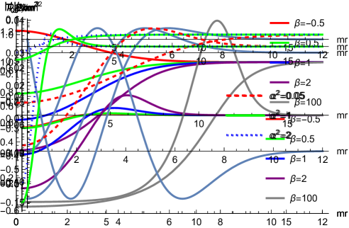
Figure 2: Angular momentum density $\mathcal{J}$ of the inhomogeneous broken vacuum in unit of $\kappa m^{2}$ for a Gaussian impurity (3.37) with $\alpha^{-2}=20$ and $\beta=1$.

The electric and the magnetic fields are also nonvanishing, which can be calculated from (2.13) and (2.11). The electric field has nonvanishing radial component $E_{r}$,

$$E_{r}=\frac{1}{\kappa}\frac{d}{dr}(|\phi|^{2}-v^{2}).$$ (3.43)

Similarly, the magnetic field is nonzero since the vacuum solution is not simply given by $|\phi|^{2}=v(\boldsymbol{x})^{2}$, although the entire magnetic flux $\Phi_{B}$ as well as the charge $Q_{\textrm{U(1)}}$ should be zero for the vacuum solution. We plot the these fields in Figure 3.

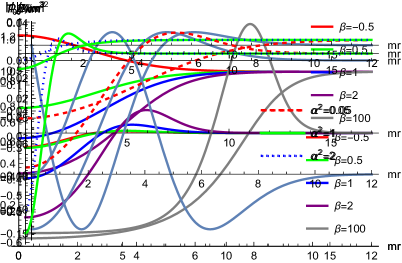
Figure 3: (a) The electric field and (b) the magnetic field of the inhomogeneous broken vacuum in unit of $m^{2}$ for a Gaussian impurity (3.37) with $\alpha^{-2}=20$ and $\beta=1$.

One can obtain a similar result when the size parameter $\alpha$ is changed. See Figure 4.

Figure 4: (a) Amplitudes of the scalar field of the inhomogeneous broken vacuum for a Gaussian impurity (3.37) with $\beta=1$ and various $\alpha$. (b) Energy densities $T_{00}$ of the vacuum in unit of $\kappa m^{3}$.

4 BPS Solitons with Inhomogeneous Mass

We are now going to discuss solutions of Bogomolny equations (2.16) and (2.18) with nonzero energies. Let us first recall the solutions in the usual homogeneous case with $\sigma(\boldsymbol{x})=0$. Thanks to the sextic potential with degenerate vacua $|\phi|=0$ and $|\phi|=v_{0}$, the equations support rich soliton spectrum such as topological vortices, nontopological solitons (Q-balls), and nontopological vortices (Q-vortices) [27, 20, 21]. Since the inhomogeneity considered here is local and does not change the essential vacuum structure as seen in the previous section, we expect that the same type of solitons exist in inhomogeneous theories. In [28], it was argued that topological vortices with positive vorticities exist if the source $\sigma(\boldsymbol{x})$ is square-integrable.

In this section we first study rotationally symmetric solutions with Gaussian-type inhomogeneity (3.37). In particular, we mainly consider the case $\beta=1$ so that $v^{2}(\boldsymbol{x})=0$ at the origin and could affect the behavior of solutions near the origin. Then at the end of the section, we discuss solutions without rotational symmetry.

The relevant ansatz would be

$$\phi =|\phi(r)|e^{in\theta},$$

$$A^{i} =-\epsilon^{ij}x_{j}\frac{A_{\theta}(r)}{r^{2}}.$$ (4.44)

Here $n$ is the vorticity of the solution and should be a nonnegative integer as discussed at the end of Section 2. For regular solutions, we should have $A_{\theta}(0)=0$ and $|\phi(r)|\sim r^{n}$ as $r\rightarrow 0$. This ansatz is suitable for obtaining solutions with $n$ zeros of $\phi$ all located at the origin. Then the Bogomolny equations (2.16) and (2.18) become

$$\frac{d|\phi|}{dr} =\frac{1}{r}(n-A_{\theta})|\phi|,$$ (4.45)

$$\frac{1}{r}\frac{dA_{\theta}}{dr} =\frac{2}{\kappa^{2}}|\phi|^{2}[v_{0}^{2}+\sigma(r)-|\phi|^{2}].$$ (4.46)

Combining the two equations, we can also obtain a single second-order equation (3.40) for $r>0$.

To find finite energy solutions, we need to impose the boundary conditions that $|\phi|$ approaches the vacuum value as $r\rightarrow\infty$,

$$|\phi(r)| \sim v_{0}, A_{\theta}(r)\sim n\qquad$$ (broken phase),

$$|\phi(r)| \sim r^{-\varepsilon}, A_{\theta}(r)\sim n+\varepsilon\qquad$$ (symmetric phase), (4.47)

where $\varepsilon$ is some positive constant and we have used (4.45) to get boundary conditions for $A_{\theta}$. With these ansatz, the magnetic flux $\Phi_{B}$ and the angular momentum $J$ in (3.36) can be determined as

$$\Phi_{B} =2\pi[A_{\theta}(\infty)-A_{\theta}(0)]=2\pi(n+\varepsilon),$$

$$J =\pi\kappa[(n-A_{\theta}(\infty))^{2}-(n-A_{\theta}(0))^{2}]=\pi\kappa(\varepsilon^{2}-n^{2}),$$ (4.48)

where we put $\varepsilon=0$ for broken phase. Note that these values are the same as those of the homogeneous case [27], independent of the details of the inhomogeneity $\sigma(r)$, since they are completely determined by the boundary conditions.

It is convenient to classify the solutions by asymptotic values of $|\phi|$ and also by the vorticity $n$.

1. $|\phi(\infty)|=v_{0}$ and $n=0$: This is nothing but the vacuum solution discussed in section 3.

2. $|\phi(\infty)|=v_{0}$ and $n\neq 0$: These are topological vortex solutions [20, 21, 28] deformed in the inhomogeneous background $\sigma(\boldsymbol{x})$.

3. $|\phi(\infty)|=0$ and $n=0$: Other than the trivial symmetric vacuum $\phi=0$, these are nontopological solitons (Q-balls) [27] deformed by $\sigma(\boldsymbol{x})$.

4. $|\phi(\infty)|=0$ and $n\neq 0$: These solutions are nontopological vortices and are called Q-vortices [27] deformed by $\sigma(\boldsymbol{x})$.

In the following we discuss each solution in detail.

4.1 Topological vortices

As in the homogeneous case $\sigma(\boldsymbol{x})=0$, $|\phi(\infty)|=v_{0}$ and $n\neq 0$ correspond to topological vortex solutions [28]. At large distances, the asymptotic behaviors of the solutions are the same as (3.42). Near the origin, we obtain

$$|\phi| \approx a\,v_{0}\,(mr)^{n}\left[1-\frac{a^{2}(\alpha^{2}-a^{2}\delta_{n1})}{8(n+2)^{2}}(mr)^{2n+4}+\frac{a^{2}(\alpha^{4}+2a^{2}\delta_{n2})}{16(n+3)^{2}}(mr)^{2n+6}+\cdots\right],$$

$$A_{\theta} \approx\frac{a^{2}(\alpha^{2}-a^{2}\delta_{n1})}{4(n+2)}(mr)^{2n+4}-\frac{a^{2}(\alpha^{4}+2a^{2}\delta_{n2})}{8(n+3)}(mr)^{2n+6}+\cdots$$ (4.49)

for some constant $a$ with $\beta=1$. Except the leading term $r^{n}$ in $|\phi|$, the expansion (4.49) is completely different from the homogeneous case [20, 21] which corresponds to $\alpha\rightarrow\infty$ limit. This is because the source term (3.37) with $\beta=1$ cancels $v_{0}$ at the origin so that $v(0)=0$. Nevertheless, topological vortex solutions can be obtained by adjusting the parameters $a$ and $b$. In fact, if the parameter $a$ is chosen too large, $|\phi|$ reaches $v_{0}$ at some finite $r$ and then diverges. If $a$ is chosen too small, $|\phi|$ goes to zero asymptotically. Then, there should be a unique value $a=a_{n}^{v}$ for each vorticity $n$ which satisfies the boundary condition $|\phi(\infty)|=v_{0}$.

In Figure 5, we plot numerical solutions for $n=1,3$ and 6 as illustrations. We also compare them with the vacuum solution discussed in section 3 as well as with $n=1$ solution of the homogeneous theory ($\sigma=0$). We can easily see the effect of $\sigma$ in two $n=1$ solutions. The energy densities $T_{00}$ of the vortex solutions vanish at the origin except $n=1$ case. Apparently, this is the same behavior as in the homogeneous case. Note, however, that $T_{00}<0$ for the vacuum solution. Thus, in this sense, the vortex contribution to energy relative to the vacuum is nonzero positive near the origin, which is to be contrasted with the homogeneous case where $T_{00}=0$ at the origin for both the vacuum and the vortices with $n>1$.

5

Figure 5: (a) Amplitudes of the scalar field of topological vortices for a Gaussian impurity (3.37) with $\alpha^{-2}=20$ and $\beta=1$. As a reference, $n=1$ vortex with $\sigma=0$ is also plotted as a dotted line. (b) Energy densities $T_{00}$ of the topological vortices in unit of $\kappa m^{3}$.

We also plot the magnetic field and the angular momentum density in Figure 6. Although the magnetic fields of the vortices vanish at the origin and appear ring-shaped, the net vortex contributions do not, as the magnetic field of the vacuum is negative near the origin, which is again different from the homogeneous system. Therefore, one may say that the vortices restore the energy and the magnetic field at the impurity position which are depleted and expelled outwards by the impurity $\sigma(\boldsymbol{x})$.

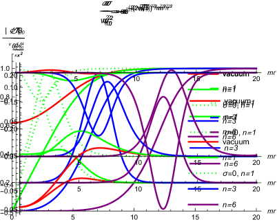
Figure 6: (a) Magnetic fields of topological vortices in unit of $m^{2}$ for a Gaussian impurity (3.37) with $\alpha^{-2}=20$ and $\beta=1$. As a reference, $n=1$ vortex with $\sigma=0$ is also plotted as a dotted line. (b) Angular Momentum densities of topological vortices in unit of $\kappa m^{2}$.

The objects are spinning with negative angular momentum $J=-\pi\kappa n^{2}$. As in section 3, we can understand the sign from $\mathcal{J}$ in (2.26), where the factor $|\phi|^{2}-v^{2}(\boldsymbol{x})$ is always negative for topological vortices while $d|\phi|/dr$ is positive.

4.2 Nontopological solitons

When $|\phi(\infty)|=0$ with $n=0$, an obvious solution is the trivial symmetric vacuum solution $\phi=0$ as discussed in section 3. There exist, however, nontopological soliton solutions characterized by the value of the magnetic flux $\Phi_{B}=2\pi\varepsilon$ as shown in (4). By the Gauss’ law, this object also has a nonzero charge $Q_{\text{U}(1)}=\kappa\Phi_{B}=2\pi\kappa\varepsilon$, and is also called a Q-ball.

Since $|\phi(0)|$ is nonvanishing, the behavior of the solution near the origin is the same as the broken vacuum discussed in section 3, i.e., it is given by (3). The constant $a$, however, should be smaller than $a_{v}$ in this case so that $|\phi|$ decays to zero asymptotically. Any nonzero positive $a$ smaller than $a_{v}$ should yield a Q-ball solution. At large distances, the impurity $\sigma$ decays exponentially and should have no effect on the power-law behavior as $r\rightarrow\infty$. Thus it is identical to the homogeneous case in [27], namely,

$$|\phi| \approx\frac{b}{(mr)^{\varepsilon}}\left[1-\frac{b^{2}}{8(\varepsilon-1)^{2}(mr)^{2\varepsilon-2}}+\cdots\right],$$

$$A_{\theta} \approx\varepsilon-\frac{b^{2}}{4(\varepsilon-1)(mr)^{2\varepsilon-2}}+\cdots,$$ (4.50)

for some constants $b$ and $\varepsilon$ which will be determined by $a$. Recall that the coefficient of the quadratic term in (3) is always positive with $\beta=1$ unlike the homogeneous case where $\beta=0$. Then $|\phi|$ should increase near the origin as a function of $r$ and then decreases to zero as $r$ goes to infinity. Such behaviors are clearly seen in Figure 7 which is obtained numerically.

Figure 7: Amplitudes of the scalar field of nontopological solitons (Q-balls) for various $a$ in (4.49) for a Gaussian impurity (3.37) with $\alpha^{-2}=20$ and $\beta=1$.

In this figure, we can also notice that solutions with large $a$ corresponds to large $\varepsilon$ or large $\Phi_{B}$. We have numerically obtained the relation between $\varepsilon$ and $a$ which is shown in Figure 8.

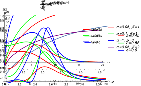
Figure 8: Scalar amplitude at the origin $a$ as a function of the decay exponent $\varepsilon$ for a Gaussian impurity (3.37) with various $\alpha$ and $\beta$. Note that the lower limits of $\varepsilon$ are almost 2 which is the Liouville limit in the homogeneous theory.

In the homogeneous case, it is known [27] that $\varepsilon>2$ with $\varepsilon=2$ being small-$|\phi|$ limit, where the Bogomolny equation (2.34) becomes the Liouville equation since $|\phi|^{2}$ can be neglected in the expression $|\phi|^{2}-v^{2}$ for constant $v$. In the present case, this approximation is no longer valid since $v^{2}(\boldsymbol{x})$ can be smaller than $|\phi|^{2}$ near the origin for $\beta\geq 1$. Nevertheless, it is clear that there should be a lower bound for $\varepsilon$ because $\varepsilon>1$ for the energy to be finite. We tried to obtain the bound numerically for various $\alpha$ and $\beta$, expecting that it would vary as a function of them. We find that, for $\beta>0$, the lower bound does not change much from $\varepsilon=2$ as seen in Figure 8, while it tends to be less than 2 for $\beta<0$. The reason behind this phenomenon is not clear to us at the moment. We leave this issue as a future problem.

The magnetic flux and the angular momentum are given by $\Phi_{B}=2\pi\varepsilon$ and $J=\pi\kappa\varepsilon^{2}$, respectively. Then, they have also the corresponding lower bounds irrespective of $\sigma$. In Figure 9, we plot the magnetic fields and the angular momentum densities for some typical values of $a$ with $\alpha^{-2}=20$ and $\beta=1$. Note that the angular momentum density $\mathcal{J}$ is mostly positive, which can be understood from the expression (2.26) since $|\phi|$ decays to zero for most of the region.

Figure 9: (a) Magnetic fields of nontopological solitons in unit of $m^{2}$ for a Gaussian impurity (3.37) with $\alpha^{-2}=20$ and $\beta=1$. (b) Angular Momentum densities of nontopological solitons in unit of $\kappa m^{2}$.

Since the solutions are in the topologically trivial sector, one has to worry about their stability against decaying into other excitations including perturbative charged particles. From (2.15), we see that the energy is given by

$$E=m_{\phi}|Q_{\text{U}(1)}|,$$ (4.51)

where $m_{\phi}$ is the scalar mass (2.3) in the symmetric phase. Then the energy per unit charge is the same as that of the elementary excitation. It implies that the nontopological soliton is marginally stable, just as in the homogeneous case [27].

4.3 Nontopological vortices

We get nontopological vortices or Q-vortices with asymptotically decaying $n\neq 0$ solutions. They may be considered as hybrids of previous two cases, i.e., nontopological solitons with vortices embedded at the center. The series expansion near the origin is the same as (4.49) where the constant $a$ should now be smaller than $a_{n}^{v}$ for each $n$ which is the value for topological vortices. The asymptotic behavior is again given by (4.2).

In Figure 10, we plot numerical solutions for $n=1,2$ and 3. Double-ring shape of the energy density $T_{00}$ shows that these solutions are hybrids of vortices and Q-balls of magnetic flux $\Phi_{B}=2\pi(n+\varepsilon)$. The solutions are also marginally stable against decaying into elementary excitations with energy (4.51).

Figure 10: (a) Amplitudes of the scalar field of nontopological vortices for a Gaussian impurity (3.37) with $\alpha^{-2}=20$ and $\beta=1$. (b) Energy densities $T_{00}$ of the nontopological vortices in unit of $\kappa m^{3}$.

Numerically we find that if $\beta>0$ the lower bound of $\varepsilon$ does not change much from $n+2$ which is the value obtained in Liouville approximation, as in the case of nontopological solitons discussed above. We plot $\varepsilon$ vs $a$ for $n=1,2$ in Figure 11.

Figure 11: Parameter $a$ in (4.49) as a function of the decay exponent $\varepsilon$ for a Gaussian impurity (3.37) with different $n$ and $\alpha$. The lower limits of $\varepsilon$ are almost $n+2$ which is the Liouville limit in the homogeneous theory.

Nontopological vortices are spinning with angular momentum (4) which manifestly shows that it consists of two parts, namely the vortex contribution $-\pi\kappa^{2}n^{2}$ and the Q-ball contribution $\pi\kappa\varepsilon^{2}$. This can also be seen from the plot of the angular momentum density $\mathcal{J}$ in Figure 12. Note that the inner region (vortex part) and the outer region (Q-ball part) are spinning in different directions but the Q-ball part mostly wins since $\varepsilon>n$.

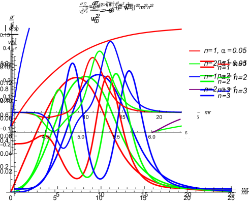
Figure 12: Angular momentum densities of nontopological vortices in unit of $\kappa m^{2}$ for a Gaussian impurity (3.37) with $\alpha^{-2}=20$ and $\beta=1$.

4.4 Solutions without rotational symmetry

So far, we have considered solutions with rotational symmetry. Here we briefly discuss general solutions which need not be rotationally symmetric. For topological vortices, the existence was shown in [28] for square integrable $\sigma(\boldsymbol{x})$. We counted the number of zero modes with the standard procedure [27] and confirmed that there are $2n$ zero modes for topological vortices with vorticity $n$ as in the homogeneous case, which are identified with the $2n$ coordinates of $n$ vortex positions. We also checked that for nontopological solutions the number of zero modes is $2(n+\hat{\varepsilon})$ regardless of the impurity $\sigma$, where $\hat{\varepsilon}$ is the largest integer less than $\varepsilon$. Thus we expect that there exist general multi-vortex solutions with arbitrary vortex points, although index analysis does not completely prove the existence, that awaits further mathematical analysis.

5 Conclusions

In this paper, we have studied the Chern-Simons Higgs model with a magnetic impurity which allows supersymmetric extension with a suitable choice of the impurity term. Compared to the homogeneous theory without an impurity, the number of supersymmetries is reduced from $\mathcal{N}=2$ to $\mathcal{N}=1$. Since the translation symmetry is broken, vacuum solutions need not be constant in this theory. We showed that, in addition to the trivial vacuum $\phi=0$ in the symmetric phase, the vacuum in the broken phase has a nontrivial profile satisfying the Bogomolny equations. It has nontrivial energy density, magnetic field and angular momentum density while its energy, magnetic flux and angular momentum remain all zero. Depending on the sign of the impurity term added to the Lagrangian, the Bogomolny equations only have vortex solutions with either positive vorticities or negative vorticities, but not both.

As an explicit example, we numerically obtained various type of rotationally symmetric soliton solutions such as (non)topological vortices and Q-balls for a Gaussian impurity. Basic properties of the solutions are similar to those in the homogeneous theory and largely independent of the detailed form of the impurity, although there are some peculiarities in nontopological solitons which are not protected by topology as discussed in section 4. It is probably due to the fact that the impurity considered here is local and does not change the essential vacuum structure. It would be interesting to see what would happen if one introduces inhomogeneities which decay more slowly or do not vanish asymptotically. In this regards, we recall that in (1+1)-dimensional supersymmetric inhomogeneous theories there is a rich spectrum of static BPS solutions [18].

In the homogeneous Chern-Simons Higgs model, there are also domain wall solutions [27] which connect the symmetric vacuum and the broken vacuum. We expect that such solutions also exist in inhomogeneous theories as long as the vacuum structure does not change. In this paper, we investigated theories with a U(1) Chern-Simons gauge field. One can consider, instead, theories with a Maxwell term [15, 16, 32] or both. The gauge field can also be nonabelian [12]. We will report the results on these issues in separate publications.

References

- [1] E. B. Bogomolny, Sov. J. Nucl. Phys. 24, 449 (1976) PRINT-76-0543 (LANDAU-INST.).
- [2] M. K. Prasad and C. M. Sommerfield, Phys. Rev. Lett. 35, 760-762 (1975) doi:10.1103/PhysRevLett.35.760
- [3] P. Di Vecchia and S. Ferrara, Nucl. Phys. B 130, 93-104 (1977) doi:10.1016/0550-3213(77)90394-7
- [4] E. Witten and D. I. Olive, Phys. Lett. B 78, 97-101 (1978) doi:10.1016/0370-2693(78)90357-X
- [5] D. Bak, M. Gutperle and S. Hirano, JHEP 05, 072 (2003) doi:10.1088/1126-6708/2003/05/072 [arXiv:hep-th/0304129 [hep-th]].
- [6] A. Clark and A. Karch, JHEP 10, 094 (2005) doi:10.1088/1126-6708/2005/10/094 [arXiv:hep-th/0506265 [hep-th]].
- [7] E. D’Hoker, J. Estes and M. Gutperle, JHEP 06, 021 (2007) doi:10.1088/1126-6708/2007/06/021 [arXiv:0705.0022 [hep-th]].
- [8] E. D’Hoker, J. Estes and M. Gutperle, Nucl. Phys. B 753, 16-41 (2006) doi:10.1016/j.nuclphysb.2006.07.001 [arXiv:hep-th/0603013 [hep-th]].
- [9] C. Kim, E. Koh and K. M. Lee, JHEP 06, 040 (2008) doi:10.1088/1126-6708/2008/06/040 [arXiv:0802.2143 [hep-th]].
- [10] C. Kim, E. Koh and K. M. Lee, Phys. Rev. D 79, 126013 (2009) doi:10.1103/PhysRevD.79.126013 [arXiv:0901.0506 [hep-th]].
- [11] K. K. Kim and O. K. Kwon, JHEP 08, 082 (2018) doi:10.1007/JHEP08(2018)082 [arXiv:1806.06963 [hep-th]].
- [12] K. K. Kim, Y. Kim, O. K. Kwon and C. Kim, JHEP 12, 153 (2019) doi:10.1007/JHEP12(2019)153 [arXiv:1910.05044 [hep-th]].
- [13] I. Arav, K. C. M. Cheung, J. P. Gauntlett, M. M. Roberts and C. Rosen, JHEP 11, 156 (2020) doi:10.1007/JHEP11(2020)156 [arXiv:2007.15095 [hep-th]].
- [14] Y. Kim, O. K. Kwon and D. D. Tolla, JHEP 12, 060 (2020) doi:10.1007/JHEP12(2020)060 [arXiv:2008.00868 [hep-th]].
- [15] A. Hook, S. Kachru and G. Torroba, JHEP 11, 004 (2013) doi:10.1007/JHEP11(2013)004 [arXiv:1308.4416 [hep-th]].
- [16] D. Tong and K. Wong, JHEP 01, 090 (2014) doi:10.1007/JHEP01(2014)090 [arXiv:1309.2644 [hep-th]].
- [17] C. Adam, J. M. Queiruga and A. Wereszczynski, JHEP 07, 164 (2019) doi:10.1007/JHEP07(2019)164 [arXiv:1901.04501 [hep-th]].
- [18] O. K. Kwon, C. Kim and Y. Kim, JHEP 01, 140 (2022) doi:10.1007/JHEP01(2022)140 [arXiv:2110.13393 [hep-th]].
- [19] J. Ho, O. K. Kwon, S. A. Park and S. H. Yi, JHEP 11, 219 (2023) doi:10.1007/JHEP11(2023)219 [arXiv:2211.05699 [hep-th]].
- [20] J. Hong, Y. Kim and P. Y. Pac, Phys. Rev. Lett. 64, 2230 (1990) doi:10.1103/PhysRevLett.64.2230
- [21] R. Jackiw and E. J. Weinberg, Phys. Rev. Lett. 64, 2234 (1990) doi:10.1103/PhysRevLett.64.2234
- [22] F. Wilczek, Phys. Rev. Lett. 48, 1144-1146 (1982) doi:10.1103/PhysRevLett.48.1144
- [23] D. P. Arovas, J. R. Schrieffer, F. Wilczek and A. Zee, Nucl. Phys. B 251, 117-126 (1985) doi:10.1016/0550-3213(85)90252-4
- [24] D. C. Tsui, H. L. Stormer and A. C. Gossard, Phys. Rev. Lett. 48, 1559-1562 (1982) doi:10.1103/PhysRevLett.48.1559
- [25] Y. H. Chen, F. Wilczek, E. Witten and B. I. Halperin, Int. J. Mod. Phys. B 3, 1001 (1989) doi:10.1142/S0217979289000725
- [26] C. Lee, K. Lee and E. J. Weinberg, Phys. Lett. B 243, 105-108 (1990) doi:10.1016/0370-2693(90)90964-8
- [27] R. Jackiw, K. Lee and E. J. Weinberg, Phys. Rev. D 42, 3488-3499 (1990) doi:10.1103/PhysRevD.42.3488
- [28] X. Han and Y. Yang, JHEP 02, 046 (2016) doi:10.1007/JHEP02(2016)046 [arXiv:1510.07077 [hep-th]].
- [29] C. Kim, C. Lee, P. Ko, B. H. Lee and H. Min, Phys. Rev. D 48, 1821-1840 (1993) doi:10.1103/PhysRevD.48.1821 [arXiv:hep-th/9303131 [hep-th]].
- [30] A. M. Jaffe and C. H. Taubes, Vortices and Monopoles: Structure of Static Gauge Theories, Birkhäuser (1980).
- [31] Y. Kim and K. M. Lee, Phys. Rev. D 49, 2041-2054 (1994) doi:10.1103/PhysRevD.49.2041 [arXiv:hep-th/9211035 [hep-th]].
- [32] Y. Kim, S. J. Jeon, O-K. Kwon, H. W. Song and C. Kim, Vacuum and Vortices in Inhomogeneous Abelian Higgs Model, to appear.