Reactive Collision Avoidance for Safe Agile Navigation

Abstract

Reactive collision avoidance is essential for agile robots navigating complex and dynamic environments, enabling real-time obstacle response. However, this task is inherently challenging because it requires a tight integration of perception, planning, and control, which traditional methods often handle separately, resulting in compounded errors and delays. This paper introduces a novel approach that unifies these tasks into a single reactive framework using solely onboard sensing and computing. Our method combines nonlinear model predictive control with adaptive control barrier functions, directly linking perception-driven constraints to real-time planning and control. Constraints are determined by using a neural network to refine noisy RGB-D data, enhancing depth accuracy, and selecting points with the minimum time-to-collision to prioritize the most immediate threats. To maintain a balance between safety and agility, a heuristic dynamically adjusts the optimization process, preventing overconstraints in real time. Extensive experiments with an agile quadrotor demonstrate effective collision avoidance across diverse indoor and outdoor environments, without requiring environment-specific tuning or explicit mapping.

Supplementary Material

Video: https://youtu.be/pUiWym4NsvA

I Introduction

Reactive collision avoidance is essential for robots navigating dynamic and unstructured environments where pre-mapped data is unavailable or unreliable [1]. This capability allows robots to perceive their surroundings and plan and execute collision-free maneuvers using real-time sensory observations, enabling them to adapt swiftly to unexpected changes such as moving obstacles or varying terrains. However, achieving reliable and efficient reactive collision avoidance remains a significant challenge due to the complexities of jointly solving perception, planning, and control [2, 3, 4, 5, 6, 7].

A primary challenge lies in embedding raw perception data into control algorithms. Sensors like RGB-D cameras provide high-dimensional and noisy data, which are computationally expensive to process and often unreliable when directly used in control [8]. Many existing systems attempt to mitigate these issues by simplifying perception inputs or assuming ideal sensor performance [9, 10, 11, 12, 13, 14, 15]. Still, these simplifications often fall short in real-world scenarios where environmental conditions are unpredictable and sensor data is imperfect.

Jointly solving motion planning and control under perception constraints also presents substantial difficulties. Traditional methods often decouple all these tasks [16, 17, 18, 19, 20, 21, 22, 23, 24, 25, 26, 27], resulting in inefficiencies and suboptimal performance in dynamic environments. In contrast, Nonlinear Model Predictive Control (NMPC) addresses these limitations by integrating planning and control into a unified constrained optimization framework. This integration allows NMPC to directly embed safety constraints, such as obstacle avoidance and actuation limits, within its optimization process, making it particularly effective for reactive collision avoidance [28, 29, 30].

Control Barrier Functions (CBFs) have recently emerged as a widely adopted method for enforcing safety constraints in obstacle avoidance [31, 32, 33, 34, 35, 36, 37, 38, 39, 40, 41, 42, 43]. CBFs provide a formal mathematical framework that defines boundaries to prevent a system from entering unsafe states. By establishing a barrier between safe and unsafe regions of the state space, CBFs guide control inputs to maintain safety while achieving the desired task [44]. However, despite their theoretical appeal, state-of-the-art approaches often oversimplify CBFs as safety filters [34], rely on restrictive assumptions of static obstacles [35, 31, 34, 32, 33], and face computational challenges [36, 37, 38], limiting their applicability to real-world settings.

To address these challenges, we present a novel framework that integrates NMPC with dynamically adjusting high-order CBFs to jointly solve the planning and control tasks under real-time perception constraints. Our contributions are: (i) We propose a unified approach that adapts to unknown environments without relying on assumptions about obstacle characteristics or sensor performance. (ii) Our perception pipeline utilizes a monocular depth estimation neural network to enhance noisy RGB-D sensor data and identify high-risk collision points based on minimal time-to-collision. (iii) We introduce dynamically adjusting high-order CBFs that update at every NMPC iteration, allowing the system to continuously adapt its safety constraints. (iv) A heuristic is implemented to dynamically relax the optimization process based on real-time collision risk, balancing safety and performance. Extensive experiments on an agile quadrotor platform demonstrate the efficiency and effectiveness of the proposed framework in both indoor and outdoor environments, proving its real-time feasibility for applications where reactive collision avoidance is critical to ensure safety (Figure LABEL:fig:initial_figure).

II Related Work

Perception and Environment Sensing. Accurate environmental perception is crucial for reactive collision avoidance in autonomous robots, particularly when pre-mapped data is unavailable or unreliable. Traditional sensors like LiDAR and sonar have been widely used due to their precision in depth measurement [45, 46, 47, 48, 49, 50]. Still, their bulky size, high weight, and significant energy consumption make them unsuitable for small, agile platforms such as quadrotors [51]. RGB-D cameras are frequently adopted for onboard sensing as they offer a lightweight and cost-effective alternative with a wide field of view. However, these sensors often produce high-dimensional, noisy, and incomplete data due to inherent sensor limitations, adverse environmental conditions, and the variable reflectivity of different surfaces [8]. These data imperfections pose significant challenges when using perception data for motion planning and control directly.

To mitigate these challenges, recent research has increasingly focused on deep learning methods for enhancing depth perception. Techniques such as monocular depth estimation utilize visual cues including shading, texture gradients, and object boundaries, achieving strong generalization across diverse environments [52, 53, 54]. Nonetheless, these methods predominantly estimate relative depth and often struggle to accurately infer absolute depth, which is essential for precise obstacle avoidance [55]. Efforts to improve absolute depth accuracy through scale correction and environment-specific priors have been explored [56, 57, 58, 59], but these solutions often come at the cost of increased computational complexity and reduced adaptability to new environments.

Collision-Free Planning and Control. Traditional collision avoidance methods often separate planning and control, where the planner generates a collision-free path, and the controller is tasked to follow it. Common methods include potential fields [16, 17, 18], sampling-based [19, 20], motion primitives [21], and graph-search methods [22, 23]. This separation has limitations, as it ignores disturbances during the control phase and can result in paths the controller cannot feasibly execute. Additionally, decoupling leads to delays, reducing responsiveness in rapidly changing environments.

Optimization-based methods such as NMPC address these limitations by merging planning and control into a single process. NMPC predicts future states and optimizes control inputs in real-time, embedding constraints directly into the control loop, offering a well-suited framework for obstacle avoidance [9, 10, 11, 12, 13, 14]. Among the various safety constraints that can be integrated into NMPC, CBFs are particularly effective due to their formal mathematical guarantees of safety [34, 35, 36]. High-order CBFs further enhance adaptability by allowing dynamic adjustment of safety boundaries in response to changes in robot and obstacle dynamics [44]. This integrated approach, using CBFs or other safety constraints within NMPC, has demonstrated success in applications such as robotic manipulation [37], coordinated quadrotor swarms [31], and high-speed autonomous vehicles [32, 33].

Despite these advances, real-world implementation remains challenging, as many studies assume perfect sensing and known obstacle locations. Extending NMPC with safety constraints like CBFs to handle unknown, dynamic environments is essential. Integrating perception, planning, and control in a unified framework enables systems to adapt control strategies in real-time, maintaining safety without compromising performance, even with imperfect data.

Recent research has investigated learning-based methods for obstacle avoidance, focusing on approaches that either learn end-to-end policies [60, 61, 62, 63] or optimize specific components within the NMPC framework [29]. Despite their potential, these methods often struggle with challenges such as interpretability, safety compliance, high data requirements, and computational overhead, which limit their real-time applicability. Integrating learning-based techniques with NMPC and robust safety constraints offers a promising path to improve adaptability and performance, particularly in dynamic and unpredictable environments.

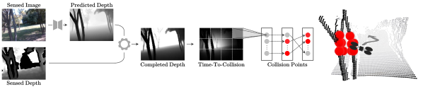
Figure 1: The proposed reactive collision avoidance framework. The perception pipeline completes sensory data by combining the sensed depth map with a predicted depth map generated from a monocular depth estimation neural network. This map is processed to compute a time-to-collision map, identifying high-risk collision points based on the robot’s velocity. The points with the highest risk of collision (highlighted in red) are identified through pooling and sorting. These high-risk points dynamically define safety constraints within the NMPC framework through CBFs, enabling safe collision-free navigation.

III Proposed Methodology

The goal is to enable an agile aerial vehicle with an RGB-D sensor to navigate safely from start to goal in unknown, dynamic environments. We do not assume prior knowledge of the environment, including obstacle shape or quantity. The robot must perceive its surroundings in real time and make decisions to avoid collisions while reaching its goal.

Figure 1 illustrates the proposed framework. The perception module processes RGB-D data to generate a depth map, which is then converted into a time-to-collision map to identify the $K$ highest-risk collision points. These points are integrated into the NMPC optimization via CBFs, allowing the controller to enforce safety constraints during flight.

III-A Depth Completion Using Monocular Depth Estimation

RGB-D sensors provide RGB images $\mathbf{I}^{t}\in\mathbb{R}^{H\times W\times 3}$ and absolute depth maps $\mathbf{D}^{t}_{\text{abs}}\in\mathbb{R}^{H\times W}$ at each time $t$. However, these depth maps often suffer from noise, incompleteness, and inaccuracies due to sensor limitations.

To address these limitations and extend the perception range beyond the baseline of the stereo camera, we employ a monocular depth estimation network $\mathcal{N}_{\text{mde}}(\mathbf{I}^{t})$ that generates a relative depth map $\mathbf{D}^{t}_{\text{rel}}\in\mathbb{R}^{H\times W}$. The observed depth map is refined by aligning it with the predicted depth using a second-order polynomial fitted to valid pixels identified by a binary mask $\mathbf{M}^{t}\in{0,1}^{H\times W}$

$$\min_{a,b,c}\sum_{(i,j)\in\mathcal{M}}\left[\mathbf{D}^{t}_{\text{abs}}(i,j)-\left(a\mathbf{D}^{t}_{\text{rel}}(i,j)^{2}+b\mathbf{D}^{t}_{\text{rel}}(i,j)+c\right)\right]^{2},$$ (1)

where $\mathcal{M}$ denotes the set of valid pixel indices defined by the mask. Our empirical analysis demonstrates that the second-order polynomial provides the most accurate fit for capturing this relationship (Section V-C).

The fitted polynomial coefficients $(a,b,c)$ allow us to compute the completed depth map

$$\mathbf{D}^{t}_{\text{com}}=a\cdot(\mathbf{D}^{t}_{\text{rel}})^{2}+b\cdot\mathbf{D}^{t}_{\text{rel}}+c\cdot\mathbf{1},$$ (2)

which minimizes noise, fills missing values, and corrects inaccuracies, providing a reliable environment representation.

III-B Fast Identification of High-Risk Collision Points

The completed depth map $\mathbf{D}^{t}_{\text{com}}$ is used to compute the time-to-collision (TTC) map $\mathbf{T}^{t}\in\mathbb{R}^{H\times W}$, which estimates collision likelihood based on the robot’s velocity vector $\mathbf{v}^{t}$. The TTC map is calculated as

$$\mathbf{T}^{t}=\frac{\mathbf{D}^{t}_{\text{com}}}{\|\mathbf{v}^{t}\cdot\mathbf{R}^{t}\|},$$ (3)

where $\mathbf{R}^{t}\in\mathbb{R}^{H\times W\times 3}$ contains the 3D ray directions from the camera through each coordinate.

TTC represents the relative distance to collision coordinates in temporal units without requiring camera calibration or specific knowledge of the environment’s structure, obstacle size, or shape [64]. This approach allows fast computation, providing the basis for quick reactive avoidance maneuvers. Despite its efficiency, the TTC map is dense, including $H\times W$ coordinates (potentially hundreds of thousands in standard camera image sizes).

To retain only the most critical coordinates, the TTC map is partitioned into non-overlapping grid cells $\mathcal{P}_{u,v}=\{(i,j)\mid uP\leq i<uP+P,\,vP\leq j<vP+P\}$ of size $P\times P$. For each cell, a min-pooling operator selects the coordinate corresponding to the smallest TTC value, effectively filtering out redundant points and retaining the most critical ones that are spatially distinct rather than overly clustered. This process forms a set of high-risk coordinates

$$\mathcal{S}^{t}_{\text{ttc}}=\left\{(i,j)\in\mathbf{T}^{t}\mid(i,j)=\operatorname*{arg\,min}_{(i,j)\in\mathcal{P}_{u,v}}\mathbf{T}^{t}(i,j),\;\forall\,u,v\right\}.$$ (4)

Next, these coordinates are filtered to retain only those representing real collision threats by comparing each pooled coordinate against the robot’s projected dimensions at the corresponding depth

$$\mathcal{S}^{t}_{\text{filt}}=\left\{(i,j)\in\mathcal{S}^{t}_{\text{ttc}}\;\middle|\;\begin{aligned} &\left|i-c_{x}\right|\leq Q_{x}f_{x}/[2\mathbf{D}^{t}_{\text{com}}(i,j)],\\ &\left|j-c_{y}\right|\leq Q_{y}f_{y}/[2\mathbf{D}^{t}_{\text{com}}(i,j)]\end{aligned}\right\},$$ (5)

where $(Q_{x},Q_{y})$ are the robot’s dimensions, $(f_{x},f_{y})$ and $(c_{x},c_{y})$ are the camera’s focal lengths and principal point.

Finally, the top-$K$ coordinates with the lowest TTC values are selected from the refined set $\mathcal{S}^{t}_{\text{filt}}$, prioritizing the highest-risk coordinates for reactive control

$$\mathcal{S}^{t}_{\text{top-}K}=\operatorname*{arg\,min}_{\begin{subarray}{c}\mathcal{S^{\prime}}^{t}_{\text{filt}}\subseteq\mathcal{S}^{t}_{\text{filt}},|\mathcal{S^{\prime}}^{t}_{\text{filt}}|=K\end{subarray}}\sum_{(i,j)\in\mathcal{S^{\prime}}^{t}_{\text{filt}}}\mathbf{T}^{t}(i,j),$$ (6)

where $\mathcal{S^{\prime}}^{t}_{\text{filt}}$ is any subset of $\mathcal{S}^{t}_{\text{filt}}$ containing $K$ coordinates. The pixel coordinates are then transformed into 3D points in the camera frame $\mathcal{C}$

$$\mathcal{S}^{t}_{\mathcal{C}}=\left\{\left(\frac{(i-c_{x})z}{f_{x}},\frac{(j-c_{y})z}{f_{y}},z\right)\;\middle|\;\begin{aligned} &z=\mathbf{D}^{t}_{\text{com}}(i,j),\\ &(i,j)\in\mathcal{S}^{t}_{\text{top-}K}\end{aligned}\right\}.$$ (7)

These 3D points are finally converted from the camera frame $\mathcal{C}$ to the body $\mathcal{B}$ and world $\mathcal{W}$ frames:

$$\mathcal{S}^{t}_{\text{W}}=\left\{\mathbf{R}_{\mathcal{WB}}\cdot\left(\mathbf{R}_{\mathcal{BC}}\cdot\mathbf{s}_{\mathcal{C}}+\mathbf{t}_{\mathcal{BC}}\right)+\mathbf{t}_{\mathcal{WB}}\;\middle|\;\mathbf{s}_{\mathcal{C}}\in\mathcal{S}^{t}_{\mathcal{C}}\right\},$$ (8)

where $\mathbf{R}_{\mathcal{BC}}$ and $\mathbf{t}_{\mathcal{BC}}$ are the rotation matrix and translation vector from the camera frame to the body frame, $\mathbf{R}_{\mathcal{WB}}$ and $\mathbf{t}_{\mathcal{WB}}$ are the rotation matrix and translation vector from the body frame to the world frame.

III-C Motion Planning and Control with Safety Constraints

The NMPC framework computes optimal control inputs that minimize trajectory deviations while ensuring collision avoidance. The state vector is defined as

$$\mathbf{x}=\begin{bmatrix}\mathbf{p}^{\top}_{\mathcal{W}}&\mathbf{v}^{\top}_{\mathcal{W}}&\mathbf{R}^{\top}_{\mathcal{BW}}&\bm{\omega}^{\top}_{\mathcal{B}}\end{bmatrix}^{\top},$$

where $\mathbf{p}$ is the system’s position in $\mathcal{W}$, $\mathbf{v}$ the linear velocity in $\mathcal{W}$, $\mathbf{R}$ the orientation from $\mathcal{B}$ to $\mathcal{W}$, and $\bm{\omega}$ the angular velocity in $\mathcal{B}$. This state forms a flexible representation for general aerial robots. The control input vector, denoted by $\mathbf{u}$, is used to influence the system’s dynamics $\mathbf{x}^{t+1}=f(\mathbf{x}^{t},\mathbf{u}^{t})$.

To ensure safety, we employ second-order CBFs for each high-risk point $\mathbf{q}^{t}_{\mathcal{W}}\in\mathcal{S}^{t}_{\mathcal{W}}$ identified from perception data. These CBFs constrain the robot to maintain a safe distance from the obstacles. Each safety constraint is defined as

$$h_{k}(\mathbf{x}^{t})=\|\mathbf{q}^{t}_{\mathcal{W}}-\mathbf{p}^{t}_{\mathcal{W}}\|^{2}-r_{\text{safe}}^{2},$$ (9)

where $r_{\text{safe}}=\max\{Q_{x},Q_{y}\}+\psi$ combines the maximum dimension of the robot and a tolerance $\psi$ to accommodate estimation uncertainties. This formulation ensures that the safety set remains forward-invariant, providing a boundary that responds dynamically to both position and velocity.

The second-order CBF constraint is expressed as

$$\ddot{h}_{k}(\mathbf{x}^{t},\mathbf{u}^{t})+2\lambda\dot{h}_{k}(\mathbf{x}^{t})+\lambda^{2}h_{k}(\mathbf{x}^{t})\geq 0,$$ (10)

where the parameter $\lambda>0$ modulates the aggressiveness of the constraint enforcement, $\dot{h}_{k}(\mathbf{x}^{t})$ captures the approach rate to the safety boundary

$$\dot{h}_{k}(\mathbf{x}^{t})=2(\mathbf{q}^{t}_{\mathcal{W}}-\mathbf{p}^{t}_{\mathcal{W}})^{\top}\mathbf{v}^{t}_{\mathcal{W}},$$ (11)

and $\ddot{h}_{k}(\mathbf{x}^{t},\mathbf{u}^{t})$ reflects the influence of control inputs on the acceleration towards the boundary

$$\ddot{h}_{k}(\mathbf{x}^{t},\mathbf{u}^{t})=2\mathbf{v}^{t\top}_{\mathcal{W}}\mathbf{v}^{t}_{\mathcal{W}}+2(\mathbf{q}^{t}_{\mathcal{W}}-\mathbf{p}^{t}_{\mathcal{W}})^{\top}\dot{\mathbf{v}}_{\mathcal{W}}(\mathbf{u}),$$ (12)

with $\dot{\mathbf{v}}_{\mathcal{W}}(\mathbf{u})$ as the robot’s acceleration driven by $\mathbf{u}$.

Integrating these CBF constraints into the NMPC scheme, the optimization problem is formulated as follows

$$\min_{\begin{subarray}{c}\mathbf{x}^{t},\dots,\mathbf{x}^{t+N}\\ \mathbf{u}^{t},\dots,\mathbf{u}^{t+N-1}\end{subarray}}\sum_{j=0}^{N}\tilde{\mathbf{x}}^{t+j\top}\mathbf{Q}_{\mathbf{x}}^{t}\tilde{\mathbf{x}}^{t+j}+\sum_{j=0}^{N-1}\tilde{\mathbf{u}}^{t+j\top}\mathbf{Q}_{\mathbf{u}}^{t}\tilde{\mathbf{u}}^{t+j},$$ (13)

where $\tilde{\mathbf{x}}^{t+j}=\mathbf{x}_{\mathrm{des}}^{t+j}-\mathbf{x}^{t+j}$ and $\tilde{\mathbf{u}}^{t+j}=\mathbf{u}_{\mathrm{des}}^{t+j}-\mathbf{u}^{t+j}$ represent the deviations between desired and actual states and inputs. The constraints applied $\forall j\in[0,N]$ and $\forall k\in[0,K)$ are

$$\mathbf{x}^{t}=\hat{\mathbf{x}}^{t},$$ (14a)

$$\mathbf{x}^{t+1+j}=f(\mathbf{x}^{t+j},\mathbf{u}^{t+j}),$$ (14b)

$$\mathbf{x}_{\min}\leq\mathbf{x}^{t+j}\leq\mathbf{x}_{\max},$$ (14c)

$$\mathbf{u}_{\min}\leq\mathbf{u}^{t+j}\leq\mathbf{u}_{\max},$$ (14d)

$$\ddot{h}_{k}(\mathbf{x}^{t+j},\mathbf{u}^{t+j})+2\lambda\dot{h}_{k}(\mathbf{x}^{t+j})+\lambda^{2}h_{k}(\mathbf{x}^{t+j})\geq 0,$$ (14e)

where $\mathbf{Q}^{t}_{\mathbf{x}}$ and $\mathbf{Q}^{t}_{\mathbf{u}}$ are positive semi-definite weight matrices, and $\hat{\mathbf{x}}^{t}$ is the current state estimate. Importantly, the CBFs are dynamically adjusted at each NMPC iteration, allowing the robot to adapt its trajectory to avoid obstacles and maintain safety even when there are drifts in state estimation.

When $K$ is large, the optimization problem may become overconstrained, forcing the NMPC to incur high costs to maintain reference tracking while satisfying all safety constraints. To prioritize safety, it is crucial to relax the tracking requirements, allowing a greater margin of error in trajectory performance. To address this challenge, we propose a heuristic that dynamically adjusts the NMPC cost function. First, we identify the point with the lowest TTC

$$(i^{*},j^{*})=\operatorname*{arg\,min}_{(i,j)\in\mathcal{S}^{t}_{\text{ttc}}}\mathbf{T}^{t}(i,j).$$ (15)

Next, the TTC is normalized using a sigmoid function to modulate its impact on the control objectives

$$\nu^{t}=(1+\exp\{-a(\mathbf{T}^{t}(i^{*},j^{*})-b)\})^{-1},$$ (16)

where the parameters $a$ and $b$ adjust the sigmoid’s sensitivity, balancing collision avoidance with control performance.

Finally, we adjust the NMPC weight matrices as follows

$$\mathbf{Q}_{\mathbf{x}}^{t} =\bar{\mathbf{Q}}_{\mathbf{x}}\cdot\nu^{t}\leavevmode\nobreak\ \leavevmode\nobreak\ \leavevmode\nobreak\ \text{and}\leavevmode\nobreak\ \leavevmode\nobreak\ \leavevmode\nobreak\ \mathbf{Q}_{\mathbf{u}}^{t} =\bar{\mathbf{Q}}_{\mathbf{u}},$$ (17)

where $\bar{\mathbf{Q}}_{\mathbf{x}}$ and $\bar{\mathbf{Q}}_{\mathbf{u}}$ are the traditional fixed weight matrices in NMPC tuned for trajectory tracking [65].

Figure 2: Experimental results demonstrating reactive collision avoidance in unknown and cluttered indoor environments. (Top row): A composite image showing the quadrotor navigating various indoor settings with unknown obstacles. (Middle row): Top-down views illustrating the reference paths and the actual collision-free paths tracked by the quadrotor. High-risk points identified during navigation are highlighted, showing the system’s responsiveness to potential collisions. (Bottom row): Graphs of the minimum values of collision-avoidance CBFs over time. The non-negative values indicate successful enforcement of safety constraints, ensuring obstacle avoidance throughout the experiment.

IV Experimental Setup and Implementation

System. Our quadrotor weighs $1.2\leavevmode\nobreak\ $\mathrm{k}\mathrm{g}$$ with a thrust-to-weight ratio of $4$ and a motor span of $25\leavevmode\nobreak\ $\mathrm{c}\mathrm{m}$$. Powered by NVIDIA Jetson Orin NX, it processes tasks onboard. A forward-facing Intel RealSense D435i captures $320\times 240$ frames. The NMPC module runs at $200\leavevmode\nobreak\ $\mathrm{H}\mathrm{z}$$ per state estimation, and CBFs update at $60\leavevmode\nobreak\ $\mathrm{H}\mathrm{z}$$ after each RGB-D frame.

Facility. Experiments took place in the ARPL indoor lab at New York University and in outdoor fields in New York State. The indoor space ($10\times 6\times 3\leavevmode\nobreak\ $\mathrm{m}^{3}$$) featured controlled lighting and static obstacles like poles and bars. Outdoor tests included natural (trees) and artificial (soccer goals) obstacles under varying weather and light conditions to test robustness.

Localization. Indoor localization used a Vicon motion capture system, providing sub-millimeter accuracy at $200\leavevmode\nobreak\ $\mathrm{H}\mathrm{z}$$. Outdoor experiments relied on a GPS u-Blox Neo-M9N module fused with IMU data via an Extended Kalman Filter (EKF), providing position updates at $100\leavevmode\nobreak\ $\mathrm{H}\mathrm{z}$$.

Perception. Depth data was acquired with the Intel RealSense D435i using the HighAccuracy setting [8], though the sensor produced incomplete data around edges and reflective surfaces. Monocular depth estimation used DepthAnythingV2 [59] with a Vision Transformer (ViT-S) backbone, optimized for NVIDIA Jetson using TensorRT, reducing inference time to $19\leavevmode\nobreak\ $\mathrm{m}\mathrm{s}$/\text{frame}$. Collision points were identified using a pooling kernel of size $P=17$, downsampling depth data to highlight the top $K=10$ high-risk coordinates. These were projected into 3D, transformed into the world frame, and modeled as CBF constraints with a safety gain $\lambda=2$ (selected empirically following [34]).

Planning and Control. The NMPC framework employs $10$ shooting steps over a $1\leavevmode\nobreak\ $\mathrm{s}$$ prediction horizon, solved using sequential quadratic programming via acados[66], with a Gauss-Newton Hessian approximation and stabilization through Levenberg-Marquardt regularization. The control input vector $\mathbf{u}$ consists of the $4$ motor thrusts, governed by a dynamic model detailed in previous works[67, 68, 69]. The planned trajectory is generated using a min-jerk trajectory planner to ensure smooth transitions, while the desired control actions are derived through differential flatness principles. State and input weights are meticulously tuned for precise trajectory tracking. The NMPC operates efficiently with $10$ active CBF constraints—empirically validated as sufficient for our experiments—achieving average computation times of $2\leavevmode\nobreak\ $\mathrm{m}\mathrm{s}$$ per iteration.

V Results and Performance Evaluation

We evaluate the proposed approach through experiments in cluttered indoor and outdoor environments. In indoor tests, the system is exposed to diverse obstacle configurations, including varying shapes, sizes, and densities, demonstrating its ability to generalize and maintain real-time performance with adjusting CBFs, ensuring safe navigation without prior knowledge of the environment. Outdoor experiments focus on agile reactive collision avoidance to maneuver the robot through trees and around the poles of a soccer goal. For further visual insights, please refer to the video.

Additionally, we analyze the effects of different polynomial orders for depth completion and the computational complexity for different camera resolutions and number of constraints.

V-A Real-Time Performance in Cluttered Indoor Environments

We evaluate the system’s performance in various cluttered indoor settings with diverse obstacle configurations, including styrofoam cuboids, mats with contrasting and ground-matching textures, room dividers, and mannequins. To further assess the robustness of the perception pipeline, we conduct tests also under low-light conditions. Detailed results and environment setups are depicted in Figure 2.

The quadrotor successfully navigates these complex scenarios without pre-tuning or prior adjustments to the perception, planning, or control modules, demonstrating the effectiveness and adaptability of the integrated NMPC with dynamically adjusting CBFs. Throughout all tests, CBF values consistently stayed above the safety thresholds, confirming the system’s ability to maintain safety constraints even in dense and low-visibility environments.

V-B Agile Safe Navigation in Outdoor Settings

We evaluate the system’s performance in outdoor environments when navigating through forest obstacles and maneuvering around the poles of a soccer goal. These setups test the system’s reactive collision avoidance capabilities, with the forest scenario presenting a cluttered environment and the soccer goal involving narrow passages and sudden obstacles. Results are shown in Figure LABEL:fig:initial_figure and Figure 3.

The quadrotor demonstrates agile safe flight with speeds up to $7.2\leavevmode\nobreak\ $\mathrm{m}\mathrm{/}\mathrm{s}$$, highlighting the system’s robustness and adaptability in complex outdoor settings. Testing outdoors introduces challenges such as variable lighting, dynamic elements like wind, and inconsistent terrain that impact sensor performance and reliability. A critical aspect of these experiments is addressing the perception limitations of the Intel RealSense D435i, which measures depth up to $3\leavevmode\nobreak\ $\mathrm{m}$$. By enhancing raw depth data with a monocular depth estimation network, the system extends its perception range, allowing for earlier obstacle detection and improved responsiveness.

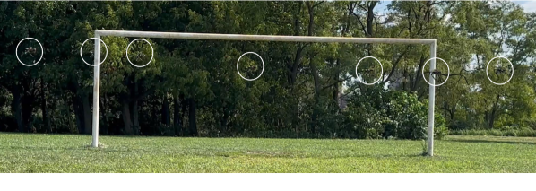
Figure 3: Safe navigation through soccer goal’s poles. The quadrotor successfully navigates through narrow passages of a soccer goal, demonstrating its reactive collision avoidance capabilities in a real-world outdoor experiment.

V-C Analysis: Polynomial Order for Depth Completion

We evaluate the impact of polynomial order on depth completion accuracy using NYUv2 [70] for indoor and KITTI [71] for outdoor data. The ground truth depth maps serve as sensed depth, and different polynomial orders are fitted to the monocular depth estimates and ground truth to determine the optimal degree for our experiments. Key metrics include Root Mean Square Error (RMSE), which highlights larger depth discrepancies, and Absolute Relative Error (AbsRel), reflecting proportional accuracy.

The results in Table I indicate that the quadratic model achieves the lowest errors on both datasets, outperforming the linear model, which fails to capture non-linear variations, and the cubic model, which tends to overfit.

V-D Analysis: Computational Complexity

We analyze the computational complexity of our system by examining the trade-offs between image resolution and network inference speed, as well as the impact of the number of CBFs on NMPC run-time. The evaluation considers the mean performance across $10$ runs.

Figure 4 highlights two critical findings. The left plot shows that increasing image resolution from $160\times 120$ to $640\times 480$ dramatically increases inference time, from $7.3\leavevmode\nobreak\ $\mathrm{m}\mathrm{s}$$ to $185.1\leavevmode\nobreak\ $\mathrm{m}\mathrm{s}$$. The steep rise in computation time between $320\times 240$ and $640\times 480$ led us to choose the former resolution for our system, balancing depth estimation accuracy and real-time performance. The right plot demonstrates that the NMPC run-time scales efficiently with the number of CBFs. As the number of constraints increases from $1$ to $100$, the run-time only grows from $1.8\leavevmode\nobreak\ $\mathrm{m}\mathrm{s}$$ to $7.0\leavevmode\nobreak\ $\mathrm{m}\mathrm{s}$$, indicating that the CBFs do not significantly impact computation time. This confirms the feasibility and real-time applicability of our approach, even with multiple constraints.

Table I: Analysis on polynomial order for depth completion. Performance of different polynomial orders (linear, quadratic, and cubic) used for depth completion on the NYUv2 and KITTI datasets. The quadratic model consistently outperforms the others, achieving the best accuracy across various metrics and datasets.

Polyn.	Polyn.	NYUv2 [70]			KITTI [71]
Order	Equation	RMSE	AbsRel		RMSE	AbsRel
Linear	$y=aX+b$	2.43	0.73		5.11	0.13
Quadratic	$y=aX^{2}+bX+c$	0.39	0.08		5.25	0.13
Cubic	$y=aX^{3}+bX^{2}+cX+d$	3.01	0.81		5.37	0.13

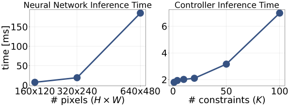
Figure 4: Analysis on computational complexity. The left plot shows increased inference time with higher image resolution, highlighting the trade-off between speed and detail. The right plot demonstrates a moderate rise in controller run-time with more CBFs, maintaining feasibility.

VI Conclusion and Future Directions

This paper presented a new obstacle avoidance framework that integrates perception constraints directly into an NMPC, enabling agile and safe navigation for autonomous robots. By jointly addressing perception, planning, and control, the proposed approach effectively navigated complex environments in real-time, as demonstrated through extensive indoor and outdoor experiments. The system’s ability to dynamically adjust control barrier functions ensured robust performance without reliance on specific environmental knowledge, making it suitable for various applications, including target tracking and autonomous exploration.

While our current work primarily focused on navigating cluttered environments with significant noise and environmental disturbances, future work will extend the system to handle dynamic obstacles by integrating obstacle kinematics prediction into the NMPC. We also plan to transition to vision-based navigation, allowing the quadrotor to rely solely on camera inputs, which will simplify the hardware and expand its applicability to compact and lightweight scenarios.

References

- [1] S. Huang, R. S. H. Teo, and K. K. Tan, “Collision avoidance of multi unmanned aerial vehicles: A review,” Annual Reviews in Control, vol. 48, pp. 147–164, 2019.
- [2] D. Falanga, P. Foehn, P. Lu, and D. Scaramuzza, “Pampc: Perception-aware model predictive control for quadrotors,” in IEEE/RSJ International Conference on Intelligent Robots and Systems (IROS), 2018, pp. 1–8.
- [3] D. Falanga, S. Kim, and D. Scaramuzza, “How fast is too fast? the role of perception latency in high-speed sense and avoid,” IEEE Robotics and Automation Letters, vol. 4, no. 2, pp. 1884–1891, 2019.
- [4] Y. Song, A. Romero, M. Müller, V. Koltun, and D. Scaramuzza, “Reaching the limit in autonomous racing: Optimal control versus reinforcement learning,” Science Robotics, vol. 8, no. 82, p. eadg1462, 2023.
- [5] A. Saviolo, P. Rao, V. Radhakrishnan, J. Xiao, and G. Loianno, “Unifying foundation models with quadrotor control for visual tracking beyond object categories,” in IEEE International Conference on Robotics and Automation (ICRA), 2024, pp. 7389–7396.
- [6] A. Nagabandi, K. Konolige, S. Levine, and V. Kumar, “Deep dynamics models for learning dexterous manipulation,” in Conference on Robot Learning. PMLR, 2020, pp. 1101–1112.
- [7] N. J. Sanket, C. D. Singh, C. Fermüller, and Y. Aloimonos, “Ajna: Generalized deep uncertainty for minimal perception on parsimonious robots,” Science Robotics, vol. 8, no. 81, p. eadd5139, 2023.
- [8] A. Grunnet-Jepsen, J. N. Sweetser, and J. Woodfill, “Best-known-methods for tuning intel® realsense™ d400 depth cameras for best performance,” Intel Corporation: Satan Clara, CA, USA, vol. 1, 2018.
- [9] X. Zhang, A. Liniger, and F. Borrelli, “Optimization-based collision avoidance,” IEEE Transactions on Control Systems Technology, vol. 29, no. 3, pp. 972–983, 2020.
- [10] B. Lindqvist, S. S. Mansouri, A.-a. Agha-mohammadi, and G. Nikolakopoulos, “Nonlinear mpc for collision avoidance and control of uavs with dynamic obstacles,” IEEE Robotics and Automation Letters, vol. 5, no. 4, pp. 6001–6008, 2020.
- [11] S. L. Herbert, M. Chen, S. Han, S. Bansal, J. F. Fisac, and C. J. Tomlin, “Fastrack: A modular framework for fast and guaranteed safe motion planning,” in IEEE 56th Annual Conference on Decision and Control (CDC), 2017, pp. 1517–1522.
- [12] J. Schulman, Y. Duan, J. Ho, A. Lee, I. Awwal, H. Bradlow, J. Pan, S. Patil, K. Goldberg, and P. Abbeel, “Motion planning with sequential convex optimization and convex collision checking,” The International Journal of Robotics Research, vol. 33, no. 9, pp. 1251–1270, 2014.
- [13] J. V. Frasch, A. Gray, M. Zanon, H. J. Ferreau, S. Sager, F. Borrelli, and M. Diehl, “An auto-generated nonlinear mpc algorithm for real-time obstacle avoidance of ground vehicles,” in European Control Conference (ECC), 2013, pp. 4136–4141.
- [14] T. Schoels, L. Palmieri, K. O. Arras, and M. Diehl, “An nmpc approach using convex inner approximations for online motion planning with guaranteed collision avoidance,” in IEEE International Conference on Robotics and Automation (ICRA), 2020, pp. 3574–3580.
- [15] V. K. Adajania, S. Zhou, A. K. Singh, and A. P. Schoellig, “Amswarm: An alternating minimization approach for safe motion planning of quadrotor swarms in cluttered environments,” in IEEE International Conference on Robotics and Automation (ICRA), 2023, pp. 1421–1427.
- [16] D. Droeschel, M. Nieuwenhuisen, M. Beul, D. Holz, J. Stückler, and S. Behnke, “Multilayered mapping and navigation for autonomous micro aerial vehicles,” Journal of Field Robotics, vol. 33, no. 4, pp. 451–475, 2016.
- [17] C. Kanellakis, S. S. Mansouri, G. Georgoulas, and G. Nikolakopoulos, “Towards autonomous surveying of underground mine using mavs,” in International Conference on Robotics in Alpe-Adria Danube Region. Springer, 2018, pp. 173–180.
- [18] J. Goricanec, A. Milas, L. Markovic, and S. Bogdan, “Collision-free trajectory following with augmented artificial potential field using uavs,” IEEE access, 2023.
- [19] S. M. LaValle and J. J. Kuffner Jr, “Randomized kinodynamic planning,” The international journal of robotics research, vol. 20, no. 5, pp. 378–400, 2001.
- [20] L. E. Kavraki, P. Svestka, J.-C. Latombe, and M. H. Overmars, “Probabilistic roadmaps for path planning in high-dimensional configuration spaces,” IEEE transactions on Robotics and Automation, vol. 12, no. 4, pp. 566–580, 1996.
- [21] M. Ginesi, D. Meli, A. Calanca, D. Dall’Alba, N. Sansonetto, and P. Fiorini, “Dynamic movement primitives: Volumetric obstacle avoidance,” in 19th International Conference on Advanced Robotics (ICAR), 2019, pp. 234–239.
- [22] L. Heng, L. Meier, P. Tanskanen, F. Fraundorfer, and M. Pollefeys, “Autonomous obstacle avoidance and maneuvering on a vision-guided mav using on-board processing,” in IEEE International Conference on Robotics and Automation (ICRA), 2011, pp. 2472–2477.
- [23] P. E. Hart, N. J. Nilsson, and B. Raphael, “A formal basis for the heuristic determination of minimum cost paths,” IEEE transactions on Systems Science and Cybernetics, vol. 4, no. 2, pp. 100–107, 1968.
- [24] G. Zhao, T. Wu, Y. Chen, and F. Gao, “Learning agility adaptation for flight in clutter,” arXiv preprint arXiv:2403.04586, 2024.
- [25] T. Marcucci, M. Petersen, D. von Wrangel, and R. Tedrake, “Motion planning around obstacles with convex optimization,” Science robotics, vol. 8, no. 84, p. eadf7843, 2023.
- [26] I. Meijer, M. Pantic, H. Oleynikova, and R. Siegwart, “Pushing the limits of reactive planning: Learning to escape local minima,” arXiv preprint arXiv:2407.13530, 2024.
- [27] J. Tordesillas, B. T. Lopez, J. Carter, J. Ware, and J. P. How, “Real-time planning with multi-fidelity models for agile flights in unknown environments,” in IEEE International Conference on Robotics and Automation (ICRA), 2019, pp. 725–731.
- [28] J. Lin, H. Zhu, and J. Alonso-Mora, “Robust vision-based obstacle avoidance for micro aerial vehicles in dynamic environments,” in IEEE International Conference on Robotics and Automation (ICRA), 2020, pp. 2682–2688.
- [29] M. Jacquet and K. Alexis, “N-mpc for deep neural network-based collision avoidance exploiting depth images,” arXiv preprint arXiv:2402.13038, 2024.
- [30] M. Krinner, A. Romero, L. Bauersfeld, M. Zeilinger, A. Carron, and D. Scaramuzza, “MPCC++: Model Predictive Contouring Control for Time-Optimal Flight with Safety Constraints,” in Proceedings of Robotics: Science and Systems, Delft, Netherlands, July 2024.
- [31] S. Wang, Y. Wang, Z. Miao, X. Wang, and W. He, “Dual model predictive control of multiple quadrotors with formation maintenance and collision avoidance,” IEEE Transactions on Industrial Electronics, 2024.
- [32] J. Zeng, B. Zhang, and K. Sreenath, “Safety-critical model predictive control with discrete-time control barrier function,” in American Control Conference (ACC), 2021, pp. 3882–3889.
- [33] T. D. Son and Q. Nguyen, “Safety-critical control for non-affine nonlinear systems with application on autonomous vehicle,” in 2019 IEEE 58th Conference on Decision and Control (CDC), 2019, pp. 7623–7628.
- [34] M. de Sa, P. Kotaru, and K. Sreenath, “Point cloud-based control barrier function regression for safe and efficient vision-based control,” in IEEE International Conference on Robotics and Automation, 2024.
- [35] R. K. Cosner, I. D. J. Rodriguez, T. G. Molnar, W. Ubellacker, Y. Yue, A. D. Ames, and K. L. Bouman, “Self-supervised online learning for safety-critical control using stereo vision,” in IEEE International Conference on Robotics and Automation (ICRA), 2022, pp. 11 487–11 493.
- [36] M. Tong, C. Dawson, and C. Fan, “Enforcing safety for vision-based controllers via control barrier functions and neural radiance fields,” in IEEE International Conference on Robotics and Automation (ICRA), 2023, pp. 10 511–10 517.
- [37] J. Liu, J. Yang, J. Mao, T. Zhu, Q. Xie, Y. Li, X. Wang, and S. Li, “Flexible active safety motion control for robotic obstacle avoidance: A cbf-guided mpc approach,” arXiv preprint arXiv:2405.12408, 2024.
- [38] M. Khan, M. Zafar, and A. Chatterjee, “Barrier functions in cascaded controller: Safe quadrotor control,” in American Control Conference (ACC), 2020, pp. 1737–1742.
- [39] B. Dai, R. Khorrambakht, P. Krishnamurthy, and F. Khorrami, “Sailing through point clouds: Safe navigation using point cloud based control barrier functions,” IEEE Robotics and Automation Letters, vol. 9, no. 9, pp. 7731–7738, 2024.
- [40] G. Niu, Q. Yang, Y. Gao, and M.-O. Pun, “Vision-based autonomous landing for unmanned aerial and ground vehicles cooperative systems,” IEEE Robotics and Automation Letters, vol. 7, no. 3, pp. 6234–6241, 2021.
- [41] M. Tayal, B. G. Goswami, K. Rajgopal, R. Singh, T. Rao, J. Keshavan, P. Jagtap, and S. Kolathaya, “A collision cone approach for control barrier functions,” arXiv preprint arXiv:2403.07043, 2024.
- [42] I. Jang and H. J. Kim, “Safe control for navigation in cluttered space using multiple lyapunov-based control barrier functions,” IEEE Robotics and Automation Letters, vol. 9, no. 3, pp. 2056–2063, 2024.
- [43] B. Dai, R. Khorrambakht, P. Krishnamurthy, V. Gonçalves, A. Tzes, and F. Khorrami, “Safe navigation and obstacle avoidance using differentiable optimization based control barrier functions,” IEEE Robotics and Automation Letters, vol. 8, no. 9, pp. 5376–5383, 2023.
- [44] A. D. Ames, S. Coogan, M. Egerstedt, G. Notomista, K. Sreenath, and P. Tabuada, “Control barrier functions: Theory and applications,” in 18th European control conference (ECC), 2019, pp. 3420–3431.
- [45] M. Harms, M. Kulkarni, N. Khedekar, M. Jacquet, and K. Alexis, “Neural control barrier functions for safe navigation,” arXiv preprint arXiv:2407.19907, 2024.
- [46] H. Ahn, J. Park, H. Bang, and Y. Kim, “Model predictive control-based multirotor three-dimensional motion planning with point cloud obstacle,” Journal of Aerospace Information Systems, vol. 19, no. 3, pp. 179–193, 2022.
- [47] K. Ebadi, L. Bernreiter, H. Biggie, G. Catt, Y. Chang, A. Chatterjee, C. E. Denniston, S.-P. Deschênes, K. Harlow, S. Khattak, L. Nogueira, M. Palieri, P. Petráček, M. Petrlík, A. Reinke, V. Krátký, S. Zhao, A.-a. Agha-mohammadi, K. Alexis, C. Heckman, K. Khosoussi, N. Kottege, B. Morrell, M. Hutter, F. Pauling, F. Pomerleau, M. Saska, S. Scherer, R. Siegwart, J. L. Williams, and L. Carlone, “Present and future of slam in extreme environments: The darpa subt challenge,” IEEE Transactions on Robotics, vol. 40, pp. 936–959, 2024.
- [48] C. S. Gadde, M. S. Gadde, N. Mohanty, and S. Sundaram, “Fast obstacle avoidance motion in small quadcopter operation in a cluttered environment,” in IEEE International Conference on Electronics, Computing and Communication Technologies (CONECCT), 2021, pp. 1–6.
- [49] S. Keyumarsi, M. W. S. Atman, and A. Gusrialdi, “Lidar-based online control barrier function synthesis for safe navigation in unknown environments,” IEEE Robotics and Automation Letters, 2023.
- [50] M. Pantic, I. Meijer, R. Bähnemann, N. Alatur, O. Andersson, C. Cadena, R. Siegwart, and L. Ott, “Obstacle avoidance using raycasting and riemannian motion policies at khz rates for mavs,” in IEEE International Conference on Robotics and Automation (ICRA), 2023, pp. 1666–1672.
- [51] J. Park and N. Cho, “Collision avoidance of hexacopter uav based on lidar data in dynamic environment,” Remote Sensing, vol. 12, no. 6, p. 975, 2020.
- [52] R. Birkl, D. Wofk, and M. Müller, “Midas v3. 1–a model zoo for robust monocular relative depth estimation,” arXiv preprint arXiv:2307.14460, 2023.
- [53] R. Ranftl, A. Bochkovskiy, and V. Koltun, “Vision transformers for dense prediction,” in Proceedings of the IEEE/CVF international conference on computer vision, 2021, pp. 12 179–12 188.
- [54] S. Wang, V. Leroy, Y. Cabon, B. Chidlovskii, and J. Revaud, “Dust3r: Geometric 3d vision made easy,” in Proceedings of the IEEE/CVF Conference on Computer Vision and Pattern Recognition, 2024, pp. 20 697–20 709.
- [55] L. Piccinelli, Y.-H. Yang, C. Sakaridis, M. Segu, S. Li, L. Van Gool, and F. Yu, “Unidepth: Universal monocular metric depth estimation,” in Proceedings of the IEEE/CVF Conference on Computer Vision and Pattern Recognition, 2024, pp. 10 106–10 116.
- [56] D. Wofk, F. Ma, T.-J. Yang, S. Karaman, and V. Sze, “Fastdepth: Fast monocular depth estimation on embedded systems,” in IEEE International Conference on Robotics and Automation (ICRA), 2019, pp. 6101–6108.
- [57] S. F. Bhat, R. Birkl, D. Wofk, P. Wonka, and M. Müller, “Zoedepth: Zero-shot transfer by combining relative and metric depth,” arXiv preprint arXiv:2302.12288, 2023.
- [58] M. Hu, W. Yin, C. Zhang, Z. Cai, X. Long, H. Chen, K. Wang, G. Yu, C. Shen, and S. Shen, “Metric3d v2: A versatile monocular geometric foundation model for zero-shot metric depth and surface normal estimation,” IEEE Transactions on Pattern Analysis and Machine Intelligence, pp. 1–18, 2024.
- [59] L. Yang, B. Kang, Z. Huang, Z. Zhao, X. Xu, J. Feng, and H. Zhao, “Depth anything v2,” arXiv preprint arXiv:2406.09414, 2024.
- [60] M. Kulkarni and K. Alexis, “Reinforcement learning for collision-free flight exploiting deep collision encoding,” in IEEE International Conference on Robotics and Automation (ICRA), 2024, pp. 15 781–15 788.
- [61] K. Hatch, J. M. Mern, and M. J. Kochenderfer, “Obstacle avoidance using a monocular camera,” in AIAA Scitech 2021 Forum, 2021, p. 0269.
- [62] J. Lu, B. Tian, H. Shen, X. Zhang, and Y. Hui, “Lpnet: A reaction-based local planner for autonomous collision avoidance using imitation learning,” IEEE Robotics and Automation Letters, 2023.
- [63] R. Brilli, M. Legittimo, F. Crocetti, M. Leomanni, M. L. Fravolini, and G. Costante, “Monocular reactive collision avoidance for mav teleoperation with deep reinforcement learning,” in IEEE International Conference on Robotics and Automation (ICRA), 2023, pp. 12 535–12 541.
- [64] G. Alenya, A. Nègre, and J. L. Crowley, “A comparison of three methods for measure of time to contact,” in IEEE/RSJ International Conference on Intelligent Robots and Systems (IROS), 2009, pp. 4565–4570.
- [65] A. Loquercio, A. Saviolo, and D. Scaramuzza, “Autotune: Controller tuning for high-speed flight,” IEEE Robotics and Automation Letters, vol. 7, no. 2, pp. 4432–4439, 2022.
- [66] R. Verschueren, G. Frison, D. Kouzoupis, J. Frey, N. van Duijkeren, A. Zanelli, B. Novoselnik, T. Albin, R. Quirynen, and M. Diehl, “acados – a modular open-source framework for fast embedded optimal control,” Mathematical Programming Computation, 2021.
- [67] A. Saviolo, G. Li, and G. Loianno, “Physics-inspired temporal learning of quadrotor dynamics for accurate model predictive trajectory tracking,” IEEE Robotics and Automation Letters, 2022.
- [68] A. Saviolo, J. Frey, A. Rathod, M. Diehl, and G. Loianno, “Active learning of discrete-time dynamics for uncertainty-aware model predictive control,” IEEE Transactions on Robotics, 2023.
- [69] A. Saviolo and G. Loianno, “Learning quadrotor dynamics for precise, safe, and agile flight control,” Annual Reviews in Control, 2023.
- [70] P. K. Nathan Silberman, Derek Hoiem and R. Fergus, “Indoor segmentation and support inference from rgbd images,” in ECCV, 2012.
- [71] A. Geiger, P. Lenz, C. Stiller, and R. Urtasun, “Vision meets robotics: The kitti dataset,” The International Journal of Robotics Research, vol. 32, no. 11, pp. 1231–1237, 2013.