Application of a Fourier-Type Series Approach based on Triangles of Constant Width to Letterforms

Abstract

In this work, we present a novel approach to type design by using Fourier-type series to generate letterforms. We construct a Fourier-type series for functions in $L^{2}(S^{1},\mathbb{C})$ based on triangles of constant width instead of circles to model the curves and shapes that define individual characters. In order to compute the coefficients of the series, we construct an isomorphism $\mathcal{R}:L^{2}(S^{1},\mathbb{C})\to L^{2}(S^{1},\mathbb{C})$ and study its application to letterforms, thus presenting an alternative to the common use of Bézier curves. The proposed method demonstrates potential for creative experimentation in modern type design.

1   Introduction

Modern type design is based on Bézier curves, which are named after Pierre Bézier (see [Bez86, BEZ77, Hos92, VTNP92, MAH⁺20, FPPM14]) although already Pierre de Casteljau worked on investigations of these curves [dC59]. Bézier curves are linear combinations of Bernstein polynomials [Ber]: A plane Bézier curve of degree $n$ is uniquely defined by $n+1$ control points $p_{0},\ldots,p_{n}\in\mathbb{R}^{2}$ and is given by the image of the map

$$t\mapsto\sum_{k=0}^{n}\binom{n}{k}t^{k}(1-t)^{n-k}p_{k},$$

where $t\in[0,1]$. These curves have therefore desirable properties since they are easy to scale or rotate and they need little computer memory. Although it is not possible to obtain all possible shapes by means of Bézier curves – it is for instance impossible to realize a circle – it can be shown that Bézier curves are dense in the space of continuous curves so that in principle, any shape can be uniformly approximated by a collection of Bézier curves (see e.g. [Nat64]).

Nowadays, the use of Bézier curves has become a standard in digital type design. TrueType fonts use piecewise quadratic Bézier curves, where as other tools such as Metafont use piecewise cubic Bézier curves [Big20].

A common criticism among type designers is that the use of Bézier curves leads typesetters to create similar fonts and symbols which are too clean. Indeed, some typeface softwares suggest improvements to the type designer – for instance, FontLab and Glyphs have features which highlight certain control points of the Bézier curve indicating “mistakes” such as high curvature or lines which are not perfectly horizontal or vertical. This leads the type designer to produce clean and similar shapes.

In another direction, Adrian Frutiger compared stems of characters to trees which are narrower on top thus describing an effect which is observed in hand-writing [Fru06]. Reproducing effects like the one mentioned with Bézier curves is much more difficult than creating e.g. a capital sans serif I which can be realized as a rectangle consisting of four straight segments and thus needing four control points only.

In this article, we investigate an approach to letterforms which is based on functional analysis and it is to our best knowledge the first instance of such an approach in the literature:

Contours of letters can be thought of one or multiple closed curves, which are homeomorphic to $S^{1}$. For simplicity we will focus on letters whose contours are topologically equivalent to $S^{1}$, making them amenable to Fourier analysis (if the contour of a letter consists of more than one connected component, each component can be treated separately). If we additionally impose that the contour of the letter is the image of a Hölder-continuous map $\mathrm{L}:S^{1}\to\mathbb{C}$, then by a theorem of Jackson [C31], it can be represented by the image the uniformly convergent series

$$\mathrm{L}(t)=\sum_{k\in\mathbb{Z}}c_{k}\mathrm{e}^{\mathrm{i}kt},$$

which, geometrically, is a sum of suitable circles. In this way, a letter can be approximated by its truncated Fourier series. As an example we have computed the Fourier series of a letter S from the Romain 20 font designed by Alice Savoie and visualized its truncated series, see Fig. 1:

$$\mathrm{L}_{m}(t)=\sum_{k\in\mathbb{Z}\atop|k|\leqslant m}c_{k}\mathrm{e}^{\mathrm{i}kt}$$

Figure 1: Truncated S for the choices $m=4,10,25$ and $m=100$.

In this paper, we will consider a series representation

$$\mathrm{L}(t)=\sum_{k\in\mathbb{Z}}\widetilde{c_{k}}\gamma(kt),$$ (1.1)

where $\gamma(t)=\mathrm{e}^{\mathrm{i}t}\left(1+a\cos(3t)-3\mathrm{i}a\sin(3t)\right)$ and $a\in[0,\frac{1}{3})$. We will show that the set $\mathcal{B}=\{\gamma(kt)\}_{k\in\mathbb{Z}}$ is a Schauder basis for $L^{2}(S^{1},\mathbb{C})$ and geometrically, (1.1) is a sum of triangles of constant width as long as $a\in(0,\frac{1}{8}]$. In order to obtain this representation, we will construct an isomorphism $\mathcal{R}:L^{2}(S^{1},\mathbb{C})\to L^{2}(S^{1},\mathbb{C})$ such that the coefficients $\widetilde{c}_{k}$ in (1.1) are precisely the Fourier-coefficients of $\mathcal{R}(\mathrm{L})$. As we will show below (Theorem 3.3), the map $\mathcal{R}$ restricts to a map $C^{k}(S^{1},\mathbb{C})\to C^{k}(S^{1},\mathbb{C})$ provided $a<1/(2^{k}(2^{k}+2))$ and the result is sharp in the sense that if $a\geqslant 1/(2^{k}(2^{k}+2))$, then the image of a $C^{k}$ function under $\mathcal{R}$ won’t be $C^{k}$ in general. This will lead to a certain roughness in the letter contours, see Section 4.

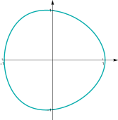
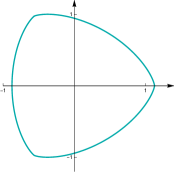
Figure 2: The images of $\gamma$ for the choices $a=\frac{1}{24}$ and $a=\frac{1}{8}$ as subsets of $\mathbb{R}^{2}\cong\mathbb{C}$

We will use the identification $S^{1}\cong\mathbb{R}/2\pi\mathbb{Z}$ throughout this article and the standard inner product of $L^{2}(S^{1},\mathbb{C})$ will be given by

$$\langle f,g\rangle=\frac{1}{2\pi}\int_{0}^{2\pi}\!\!f(t)\overline{g(t)}\,\mathrm{d}t$$

so that $\{t\mapsto\mathrm{e}^{\mathrm{i}kt}\}_{k\in\mathbb{Z}}$ is a Hilbert basis of $L^{2}(S^{1},\mathbb{C})$ with respect to $\langle\cdot{,}\cdot\rangle$ and the induced norm $\|f\|_{L^{2}}:=\sqrt{\langle f,f\rangle}$.

For $z,w\in\mathbb{C}$, we will denote by $[z,w]:=\{z(1-t)+tw,t\in[0,1]\}$ the line segment between $z$ and $w$. Similarly, we denote by $(z,w):=\{z(1-t)+tw,t\in(0,1)\}$ the corresponding line segment wihout endpoints. Recall that a set $K\subset\mathbb{C}$ is called convex, if it contains $[z,w]$ for any two points $z,w\in K$. If its interior contains $(z,w)$ for any two points $z,w\in K$, it is called strictly convex. If $\partial K$ admits a parametrization by a closed curve $\Gamma\in C^{2}(S^{1},\mathbb{C})$ with non-vanishing curvature, then $K$ is called strongly convex.

2   Parametrizations of Triangles of Constant Width

2.1   Support Functions

Boundaries of strictly convex sets admit parametrizations by so-called support functions (see [AHW21]).

If $K\subset\mathbb{C}$ is strongly convex and $\partial K$ is of class $C^{k}$, $k\geqslant 2$, then there exists a support function $p\in C^{k}(S^{1})$ such that $\partial K$ is parametrized by $t\mapsto p(t)u(t)+p^{\prime}(t)u^{\prime}(t),$ where $u(t)=\mathrm{e}^{\mathrm{i}t}$ (see [AHW21, Lemma 2.1]).

If the boundary $\partial K$ of a strictly convex set $K\subset\mathbb{C}$ is parametrized by $\Gamma:S^{1}\to\mathbb{C}$, $\Gamma(t)=p(t)u(t)+p^{\prime}(t)u^{\prime}(t)$, where $p$ is of class $C^{2}$, then we have the following elementary facts ([AHW21, p. 86]):

1. The radius of curvature is given by $\rho=p+p^{\prime\prime}$. Note that this is not trivial since a priori, $\Gamma$ is only of class $C^{1}$, see [AHW21, Corollary 2.2] for a proof of this result.
   

2. If $\rho\geqslant 0$ and $p(t+\pi)+p(t)\equiv d>0$, then $K$ is a body of constant width $d$.
   

3. The area of $K$ is given by $\displaystyle\frac{1}{2}\int_{0}^{2\pi}\!\!\left(p^{2}(t)-p^{\prime}(t)^{2}\right)\,\mathrm{d}t.\\$

4. The perimeter of $K$ (the length of $\partial K$) is given by $\displaystyle\int_{0}^{2\pi}\!\!\!\!p(t)\,\mathrm{d}t.$

2.2   Triangles of Constant Width

Let $p(t)=1+a\cos(3t)$, where $a\geqslant 0$ and $\gamma(t)=p(t)u(t)+p^{\prime}(t)u^{\prime}(t)$. For $\gamma$ to bound a strictly convex set, we need its curvature radius $\rho$ to be non-negative while being zero only in isolated points. The condition on non-negativity is given by

$$\rho(t)=p(t)+p^{\prime\prime}(t)=1-8a\cos(3t)\geqslant 0,$$

which implies $a\leqslant\frac{1}{8}$. Note that if $a<\frac{1}{8}$, then $\gamma$ bounds a strongly convex set and if $a=\frac{1}{8}$, then $\rho$ has zeros in $0,\frac{2\pi}{3}$ and $\frac{4\pi}{3}$ within $[0,2\pi)$ so that $\gamma$ bounds a strictly convex set in this case.

Since for all choices $a\in[0,\frac{1}{8}]$ we have $p(t)+p(t+\pi)\equiv 2$, the curve $\gamma$ bounds a body of constant width $2$ (see elementary fact 2)).

We will later focus on the specific choice $a=\frac{1}{8}$ for the following reason: The isoperimetric ratio of the convex body which is bounded by $\gamma$ equals

$$\frac{4\pi^{2}}{\pi(1-4a^{2})}=\frac{4\pi}{1-4a^{2}},$$

which is maximal if $a=\frac{1}{8}$. In that sense, among all the convex bodies obtained in this way, the case $a=\frac{1}{8}$ provides us with the one which is farthest from a circle with respect to its isoperimetric ratio.

3   An Isomorphism of $L^{2}(S^{1},\mathbb{C})$ based on Triangles of Constant Width

We introduce the notation $f_{k}(t)=f(kt)$ for any $f\in L^{2}(S^{1},\mathbb{C})$ and $k\in\mathbb{Z}$. Then the Fourier-series of $\gamma_{k}$ is given by

$$\gamma_{k}=u_{k}+2au_{-2k}-au_{4k}$$

which provides us with a bounded linear operator $\mathcal{T}:L^{2}(S^{1},\mathbb{C})\to L^{2}(S^{1},\mathbb{C})$ given by

$$\mathcal{T}(f)=f+2af_{-2}-af_{4}.$$ (3.1)

Indeed, if $f\in L^{2}(S^{1},\mathbb{C})$ then $\|\mathcal{T}(f)\|_{L^{2}}\leqslant(1+3a)\|f\|_{L^{2}}$. We will show that $\mathcal{T}$ admits an inverse, provided $0\leqslant a<\frac{1}{3}$:

If $a=0$, then $\mathcal{T}=\mathrm{id}_{L^{2}(S^{1},\mathbb{C})}$ and there is nothing to show. Let therefore $a>0$. If $\mathcal{T}(f)=y$ it holds that

$$f =y-2af_{-2}+af_{4}.$$ (3.2)

Since

$$f_{k}=y_{k}-af_{-2k}+2af_{4k}$$ (3.3)

for all $k\in\mathbb{Z}$ we can, using (3.3), replace $f_{-2}$ in (3.2) and obtain

$$f=y-2ay_{-2}+2a^{2}f_{-4}-2a^{2}f_{8}.$$ (3.4)

Next, $f_{-4}$ in (3.4) can be replaced using (3.3) so that proceeding inductively in this way, $f$ can eventually be expressed as a formal series

$$f(t)=\sum_{\ell=0}^{\infty}(-1)^{\ell}j_{\ell}\,y\left((-1)^{\ell}2^{\ell}t\right),$$ (3.5)

where the coefficients $j_{\ell}$ can be checked to verify a Jacobsthal-type recurrence (see for instance [Hor, Djo10, Das14, FH99]): It holds that $j_{0}=1,j_{1}=2a$ and

$$j_{n}=a(2j_{n-1}+j_{n-2})\text{ for }n\geqslant 2.$$ (3.6)

Lemma 3.1

If $a>0$, the sequence $(j_{n})_{n\in\mathbb{N}}$ with $j_{0}=1,j_{1}=2a$ verifying (3.6) admits an explicit representation

$$j_{n}=\frac{\left(a+\sqrt{a^{2}+a}\right)^{n+1}-\left(a-\sqrt{a^{2}+a}\right)^{n+1}}{2\sqrt{a^{2}+a}}$$

Proof. The real vector space $V$ of sequences $(z_{n})_{n\in\mathbb{N}}$ that solve ${z_{n}=a(2z_{n-1}+z_{n-2})}$ for all $n\geqslant 2$ admits a basis consisting of exponential functions: Let $z_{n}:=b^{n}$, where $b\neq 0$. The reccurence relation implies

$$b^{2}=a(2b+1)\Longleftrightarrow b=a\pm\sqrt{a^{2}+a}.$$

Letting $z^{\pm}_{n}=(a\pm\sqrt{a^{2}+a})^{n}$, it is straightforward to check that $\{(z^{+}_{n})_{n\in\mathbb{N}},(z^{-}_{n})_{n\in\mathbb{N}}\}$ forms a basis of $V$. Therefore, $j_{n}$ will be a linear combination of $(a+\sqrt{a^{2}+a})^{n}$ and $(a-\sqrt{a^{2}+a})^{n}$ and using $j_{0}=1$, $j_{1}=a$, we obtain the desired result. ∎

According to (3.5), the inverse of $\mathcal{T}$ is given by the formal series $\mathcal{T}^{-1}=\mathcal{R}$:

$$\mathcal{R}(y)(t)=\sum_{\ell=0}^{\infty}(-1)^{\ell}j_{\ell}\,y\left((-1)^{\ell}2^{\ell}t\right)$$

If $y\in L^{2}(S^{1},\mathbb{C})$, then $\left\|\mathcal{R}(y)\right\|_{L^{2}}\leqslant\|y\|_{L^{2}}\sum_{\ell=0}^{\infty}j_{\ell}$ so that this expression is finite if the series $\sum_{\ell=0}^{\infty}j_{\ell}$ converges. Since

$$\lim_{n\to\infty}\frac{j_{n+1}}{j_{n}}=a+\sqrt{a^{2}+a},$$

this series converges according to the ratio test if $a<\frac{1}{3}$. Replacing the $L^{2}$-norm in the above computation by the $C^{0}$-norm, it is immediate that $\mathcal{R}$ restricts to a map $C^{0}(S^{1},\mathbb{C})\to C^{0}(S^{1},\mathbb{C})$ provided $a<\frac{1}{3}$.

Summarizing we arrive at

Theorem 3.2

Let $a\in[0,\frac{1}{3})$ and let $\mathcal{T}$ be defined by equation (3.1). Then $\mathcal{T}$ is an isomorphism and its inverse $\mathcal{R}:L^{2}(S^{1},\mathbb{C})\to L^{2}(S^{1},\mathbb{C})$ is given by

$$\mathcal{R}(y)(t)=\sum_{\ell=0}^{\infty}(-1)^{\ell}\frac{\left(a+\sqrt{a^{2}+a}\right)^{\ell+1}-\left(a-\sqrt{a^{2}+a}\right)^{\ell+1}}{2\sqrt{a^{2}+a}}y\left((-1)^{\ell}2^{\ell}t\right),$$

if $a\neq 0$ and by the identity mapping on $L^{2}(S^{1},\mathbb{C})$ if $a=0$.

We will now further study under which conditions the map $\mathcal{R}$ restricts to a map $C^{k}(S^{1},\mathbb{C})\to C^{k}(S^{1},\mathbb{C})$: To this end, suppose that $y\in C^{k}(S^{1},\mathbb{C})$, then the $k$-th derivative (taken termwise) of $\mathcal{R}(y)$ is formally given by

$$\sum_{\ell=0}^{\infty}(-1)^{(k+1)\ell}2^{k\ell}j_{\ell}y^{(k)}((-1)^{\ell}2^{\ell}\,\cdot\,)$$ (3.7)

and its $C^{0}$ norm will be bounded by $\|y^{(k)}\|_{C^{0}}\sum_{\ell=0}^{\infty}2^{k\ell}j_{\ell}.$ This time, the ratio test yields

$$\lim_{n\to\infty}\frac{2^{k(n+1)}j_{n+1}}{2^{kn}j_{n}}=2^{k}\left(a+\sqrt{a^{2}+a}\right),$$

which is smaller than $1$ provided $a<\frac{1}{2^{k}(2^{k}+2)}$, so that in this case the series (3.7) converges uniformly and hence $\mathcal{R}$ restricts to $C^{k}(S^{1},\mathbb{C})\to C^{k}(S^{1},\mathbb{C})$. Summarizing we obtain

Theorem 3.3

Let $a\in[0,\frac{1}{3})$. If $a<\frac{1}{2^{k}(2^{k}+2)}$, then $\mathcal{R}$ restricts to a map $C^{k}(S^{1},\mathbb{C})\to C^{k}(S^{1},\mathbb{C})$.

This result is sharp in the following sense: According to the previous theorem, $\mathcal{R}$ restricts to a map $C^{1}(S^{1},\mathbb{R})\to C^{1}(S^{1},\mathbb{C})$ if $a<\frac{1}{8}$. If $a=\frac{1}{8}$, then the image of a $C^{1}$ function $S^{1}\to\mathbb{C}$ is not $C^{1}$ in general:

Proposition 3.4

If $y(t)=\sin(t)$ and $a=\frac{1}{8}$, then $f=\mathcal{R}(y):S^{1}\to\mathbb{C}$ is not differentiable in $t=0$.

Proof. Let $a=\frac{1}{8}$ and $y(t)=\sin(t)$, then

$$f(t)=\mathcal{R}(y)(t)=\frac{1}{3}\sum_{\ell=0}^{\infty}\frac{2^{\ell+1}+(-1)^{\ell}}{4^{\ell}}\sin\left(2^{\ell}t\right)$$

We will show that if $t_{n}=\frac{\pi}{2^{n}}$, then the sequence

$$\frac{f(t_{n})-f(0)}{t_{n}-0}=\frac{f(t_{n})}{t_{n}}$$

will diverge as $n\to\infty$.

We will use the inequality

$$\frac{2^{\ell+1}+(-1)^{\ell}}{4^{\ell}}\geqslant\frac{1}{2^{\ell}}$$

for all $\ell\in\mathbb{N}$. Since $\sin(2^{\ell}t_{n})=\sin\left(2^{\ell-n}\pi\right)$, this quantity vanishes if $\ell\geqslant n$. If $\ell<n$ we can use the inequality $\sin(x)\geqslant\frac{2}{\pi}x$ that holds on $[0,\frac{\pi}{2}]$ in order to obtain

$$f(t_{n}) \geqslant\frac{1}{3}\sum_{\ell=0}^{n-1}\frac{1}{2^{\ell}}\frac{2}{\pi}2^{\ell-n}\pi=\frac{2n}{3\cdot 2^{n}}.$$

Therefore we have

$$\frac{f(t_{n})}{t_{n}}\geqslant\frac{2^{n}}{\pi}\cdot\frac{2n}{3\cdot 2^{n}}=\frac{2n}{3\pi}\stackrel{{\scriptstyle n\to\infty}}{{\longrightarrow}}\infty.$$

∎

Remark

This previous result can be adapted in order to show that if $a=\frac{1}{2^{k}(2^{k}+2)}$, then the image under $\mathcal{R}$ of a $C^{k}$ function is not $C^{k}$ in general.

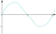
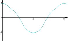
Figure 3: The graphs of $\mathcal{R}(\sin)$ and $\mathcal{R}(\cos)$ as real-valued functions if $a=\frac{1}{24}$.

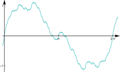
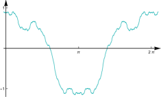
Figure 4: The graphs of $\mathcal{R}(\sin)$ and $\mathcal{R}(\cos)$ as real-valued functions if $a=\frac{1}{8}$.

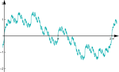
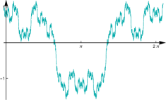
Figure 5: The graphs of $\mathcal{R}(\sin)$ and $\mathcal{R}(\cos)$ as real-valued functions if $a=\frac{1}{5}$.

Note that by construction, if $a\in[0,\frac{1}{3})$, then $\mathcal{R}(\gamma_{k})=u_{k}$ so that the we arrive at:

Proposition 3.5

If $a\in[0,\frac{1}{3})$, then set $\mathcal{B}=\{\gamma_{k}\}_{k\in\mathbb{Z}}$ is a Hilbert basis for the space $L^{2}(S^{1},\mathbb{C})$ equipped with the inner product $\mathcal{R}^{*}\langle\cdot{,}\cdot\rangle=\langle\!\langle\cdot{,}\cdot\rangle\!\rangle$.

The inner product $\langle\!\langle\cdot{,}\cdot\rangle\!\rangle$ is explicitly given by

$$\langle\!\langle f,g\rangle\!\rangle=\frac{1}{2\pi}\int_{0}^{2\pi}\mathcal{R}(f)(t)\overline{\mathcal{R}(g)(t)}\,\mathrm{d}t$$

so that a periodic function $f\in L^{2}(S^{1},\mathbb{C})$ can be represented by

$$\sum_{k\in\mathbb{Z}}\langle\!\langle f,\gamma_{k}\rangle\!\rangle\gamma_{k}.$$

Since

$$\langle\!\langle f,\gamma_{k}\rangle\!\rangle =\frac{1}{2\pi}\int_{0}^{2\pi}\mathcal{R}(f)(t)\,\overline{\mathcal{R}(\gamma_{k})(t)}\,\mathrm{d}t$$

$$=\frac{1}{2\pi}\int_{0}^{2\pi}\mathcal{R}(f)(t)\,\overline{u_{k}(t)}\,\mathrm{d}t,$$

the coefficients of $\langle\!\langle f,\gamma_{k}\rangle\!\rangle$ are precisely the Fourier-coefficients of $\mathcal{R}(f)$.

This can be restated as follows: If one defines

$$\mathcal{C}_{k}(\mathcal{F}):L^{2}(S^{1},\mathbb{C}) \to\mathbb{C}$$

$$f \mapsto\langle f,u_{k}\rangle$$

$$\mathcal{C}_{k}(\mathcal{R}):L^{2}(S^{1},\mathbb{C}) \to\mathbb{C}$$

$$f \mapsto\langle\!\langle f,\gamma_{k}\rangle\!\rangle,$$

for all $k\in\mathbb{Z}$, then the following diagram commutes:

Remark

The map $\gamma$ yields a parametrization of a closed curve in $\mathbb{C}$ for any value of $a$. It follows from Proposition 3.5, that a Fourier-type series with the unit circle replaced by $\gamma$ is available if $a<\frac{1}{3}$. We therefore also consider curves $\gamma$, where $a\in\left(\frac{1}{8},\frac{1}{3}\right)$. For $a$ in this range, $\gamma$ is no longer the boundary of a convex body but a curve with self-intersections. The image of $\gamma$ whenever $a=\frac{1}{5}$ is shown below in Fig. 6.

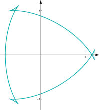
Figure 6: Image of $\gamma$ if $a=\frac{1}{5}$

4   Application to Letterforms

As long as $a\in\left[0,\frac{1}{3}\right)$, we have that $\mathcal{T}\circ\mathcal{R}=\operatorname{id}_{L^{2}(S^{1},\mathbb{C})}$. We will now introduce a truncated version of $\mathcal{R}$:

$$\mathcal{R}_{n}:L^{2}(S^{1},\mathbb{C}) \to L^{2}(S^{1},\mathbb{C})$$

$$y\mapsto\mathcal{R}_{n}(y):t \mapsto\sum_{\ell=0}^{n}(-1)^{\ell}\frac{\left(a+\sqrt{a^{2}+a}\right)^{\ell+1}-\left(a-\sqrt{a^{2}+a}\right)^{\ell+1}}{2\sqrt{a^{2}+a}}y((-1)^{\ell}2^{\ell}t)$$

The way we will use $\mathcal{R}_{n}$ in order to modify letterforms of which we think as Hölder-continuous elements $\mathrm{L}\in L^{2}(S^{1},\mathbb{C})$ is best summarized in terms of the following commutative diagram:

In this way, $(\mathcal{R}_{n}\circ\mathcal{T})(\mathrm{L})\approx\mathrm{L}$, where the approximation becomes exact as $n\to\infty$. We obtain thus different approximations as we choose different values for $a\in(0,\frac{1}{3})$ and $n\in\mathbb{N}$.

As a case study, we will choose the values $a=\frac{1}{24}$, $a=\frac{1}{8}$ and $a=\frac{1}{5}$ for different values of $n$. Note that if $a=\frac{1}{2^{k}(2^{k}+2)}$, then the coefficients in the series defining $\mathcal{R}$ take a particularly nice form, since in this case

$$\sqrt{a^{2}+a}=\frac{2^{k}+1}{2^{k}(2^{k}+2)}\in\mathbb{Q}.$$

This occurs for $a=\frac{1}{24}$ and $a=\frac{1}{8}$, which correspond to the choices $k=2$ and $k=1$.

4.1   Approximation with $a=\frac{1}{24}$

Recall that if $a=\frac{1}{24}$, then $\mathcal{R}$ restricts to a map $C^{1}(S^{1},\mathbb{C})\to C^{1}(S^{1},\mathbb{C})$ which does not in general preserve $C^{2}$ regularity according to Theorem 3.3. Here,

$$\mathcal{R}(y)(t)=\lim_{n\to\infty}\underbrace{\frac{1}{5}\sum_{\ell=0}^{n}\frac{(-\frac{1}{2})^{\ell}3^{\ell+1}+2}{6^{\ell}}\,y\left((-1)^{\ell}2^{\ell}t\right)}_{=:\mathcal{R}_{n}(y)(t)}.$$

Appliying $\mathcal{R}_{n}\circ\mathcal{T}$ to the letter S from the Romain 20 font yields the pictures in Fig. 7.

Figure 7: Application of $\mathcal{R}_{n}\circ\mathcal{T}$ to the letter S for the values $n=0,1,2,3$ if $a=\frac{1}{24}$

Even though the curve $\gamma$ for $a=\frac{1}{24}$ is relatively close to being a circle (see the left image in Fig. 2), the application of $\mathcal{R}_{n}\circ\mathcal{T}$ to the letter S produces noticeably different curves, compare to Fig. 1.

4.2   Approximation with $a=\frac{1}{8}$

If $a=\frac{1}{8}$, $\gamma$ corresponds to the triangle of constant width which is furthest from the circle with respect to its isoperimetric ratio (see Subsection 2.2) and $\mathcal{R}$ restricts to a map $C^{0}(S^{1},\mathbb{C})\to C^{0}(S^{1},\mathbb{C})$ which does not in general preserve $C^{1}$ regularity. Here,

$$\mathcal{R}(y)(t)=\lim_{n\to\infty}\underbrace{\frac{1}{3}\sum_{\ell=0}^{n}\frac{(-1)^{\ell}2^{\ell+1}+1}{4^{\ell}}\,y\left((-1)^{\ell}2^{\ell}t\right)}_{=:\mathcal{R}_{n}(y)(t)}.$$

In our case we obtain the pictures in Fig 8.

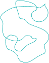
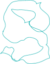
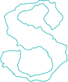
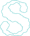
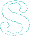
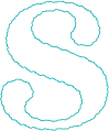
Figure 8: Application of $\mathcal{R}_{n}\circ\mathcal{T}$ to the letter S for the values $n=0,\ldots,6$ if $a=\frac{1}{8}$

It is an artefact of the regularity that the curves have angular points which give the letterforms a certain roughness like a vibrating, fuzzy object – an effect which would barely be obtainable by the use of Bézier curves.

4.3   Approximation with $a=\frac{1}{5}$

Recall that if $\frac{1}{8}<a<\frac{1}{3}$, then the image of $\gamma$ is no longer the boundary of a convex body, but $\gamma$ has self-intersections (see Figure 6). Nonetheless, $\mathcal{R}$ is still an isomorphism and preserves the continuity of mappings. If $a=\frac{1}{5}$, one obtains the following images applying $\mathcal{R}_{n}\circ\mathcal{T}$ to the letter S in Fig. 9. Here, the curves admit self-intersections and this produces a fractal-like decorative effect.

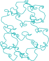
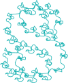
Figure 9: Application of $\mathcal{R}_{n}\circ\mathcal{T}$ to the letter S for the values $n=3,4,5,6$ if $a=\frac{1}{5}$

4.4   Conclusion

The approach to the creation of letterforms presented in this paper shows an alternative to Bézier curves. Although we do not claim that the letters we have created in this way can be used in an unmodified way nor how such an approach could be incorporated in a type design software, it shows that a functional-analytical approach, which changes letters globally and not locally, takes into account the common criticism that Bézier letters tend to be too clean. For our choice of triangles of constant width, the resulting map $\mathcal{R}$ reveals non-trivial regularity phenomena, which allow to create letterforms with self-intersections, or letters which do not have tangents in general, creating non-clean, wobbly effects. In addition, the approach provides a wealth of exploration possibilities, because other basis functions than the ones we have chosen are imaginable – for example, non-differentiable curves such as regular $n$-gons might be used as a geometric basis object.

References

- [AHW21] Jonas Allemann, Norbert Hungerbühler, and Micha Wasem. Equilibria of Plane Convex Bodies. Journal of nonlinear science, 31(5), 2021. Place: New York Publisher: Springer US.
- [Ber] S Bernstein. Proof of the theorem of Weierstrass based on the calculus of probabilities.
- [BEZ77] Pierre BEZIER. Essai de definition numerique des courbes et des surfaces experimentales: contribution a l’etude des proprietes des courbes et des surfaces parametriques polynomiales a coefficients vectoriels. s.n., S.l., 1977. OCLC: 490592464.
- [Bez86] Pierre Bezier. The Mathematical Basis of the UNISURF CAD System. Butterworth-Heinemann, USA, 1986.
- [Big20] Charles Bigelow. The Font Wars, Part 1. IEEE Annals of the History of Computing, 42(1):7–24, January 2020. Conference Name: IEEE Annals of the History of Computing.
- [C31] E. T. C. The Theory of Approximation. By Dunham Jackson. (American Mathematical Colloquium Publications, Volume XI.) Pp. viii + 178. Price not stated. 1930. (American Mathematical Society, New York.). The Mathematical Gazette, 15(216):506–507, December 1931.
- [Das14] Ahmet Dasdemir. A study on the Jacobsthal and Jacobsthal-Lucas numbers. Dicle Üniversitesi Fen Bilimleri Enstitüsü Dergisi, 3:13–18, June 2014.
- [dC59] P de Casteljau. Outillages methodes calcul. Technical report, 1959.
- [Djo10] Gospava B. Djordjević. Some Generalizations of the Jacobsthal Numbers. Filomat, 24(2):143–151, 2010. Publisher: University of Nis, Faculty of Sciences and Mathematics.
- [FH99] Piero Filipponi and Alwyn F. Horadam. Integration Sequences of Jacobsthal and Jacobsthal-Lucas Polynomials. In Fredric T. Howard, editor, Applications of Fibonacci Numbers: Volume 8, pages 129–139. Springer Netherlands, Dordrecht, 1999.
- [FPPM14] Hetal N. Fitter, Akash B. Pandey, Divyang D. Patel, and Jitendra M. Mistry. A Review on Approaches for Handling Bezier Curves in CAD for Manufacturing. Procedia Engineering, 97:1155–1166, January 2014.
- [Fru06] Adrian Frutiger. Der Mensch und seine Zeichen. Marix Verlag, 2006. Google-Books-ID: g6pDPgAACAAJ.
- [Hor] A F Horadam. JACOBSTHAL REPRESENTATION NUMBERS.
- [Hos92] Mamoru Hosaka. Bézier Curves and Control Points. In Mamoru Hosaka, editor, Modeling of Curves and Surfaces in CAD/CAM, pages 117–139. Springer, Berlin, Heidelberg, 1992.
- [MAH+20] Sidra Maqsood, Muhammad Abbas, Gang Hu, Ahmad Lutfi Amri Ramli, and Kenjiro T. Miura. A Novel Generalization of Trigonometric Bézier Curve and Surface with Shape Parameters and Its Applications. Mathematical Problems in Engineering, 2020:e4036434, May 2020. Publisher: Hindawi.
- [Nat64] I. P. Natanson. Constructive function theory. Vol. I: Uniform approximation. Translated by Alexis N. Obolensky, 1964. Published: New York: Frederick Ungar Publishing Co. IX, 232 p. (1964).
- [VTNP92] Tang Van To and Huynh Ngoc Phien. Development of Bézier-based curves. Computers in Industry, 20(1):109–115, January 1992.