Spin amplification in realistic systems

Abstract

Spin amplification is the process that ideally increases the number of excited spins if there was one excited spin to begin with. Using optimal control techniques to find classical drive pulse shapes, we show that spin amplification can be done in the previously unexplored regime with amplification times comparable to the timescale set by the interaction terms in the Hamiltonian. This is an order of magnitude faster than the previous protocols and makes spin amplification possible even with significant decoherence and inhomogeneity in the spin system. The initial spin excitation can be delocalized over the entire ensemble, which is a more typical situation when a photon is collectively absorbed by the spins. We focus on the superconducting persistent-current artificial atoms as spins, but this approach can be applied to other kinds of strongly-interacting spins, including the Rydberg atoms.

I Introduction

Control of ever larger quantum systems is essential for quantum simulation [1, 2, 3, 4], quantum sensing [5, 6, 7, 8] and error-corrected quantum computing [9, 10, 11]. Such quantum systems could be viewed as collections of spins encoded in real or artificial atoms. Instead of aiming to deliver a separate driving field for each spin, experimental complexity could be decreased by using a global drive for the entire spin ensemble [12, 13, 14, 15, 16, 17, 18, 19, 20, 21, 22]. Addressing the individual spins or spin groups could then be done by frequency or polarization selectivity and engineering of the spin-spin interactions.

One of the operations that is useful for quantum sensing is spin amplification [23, 24], which can be implemented with a global drive [17, 18, 19]. The idealized version of this operation amplifies a single excited spin into many excited spins, while keeping the ensemble with zero excited spins unchanged [see Fig. 1(a)]. This can be realized using the transverse-field Ising model with nearest-neighbor interactions. A continuous-wave weak classical field is applied such that it is off-resonant with the frequency of the spins. One excited spin shifts the frequency of the neighboring spins into resonance with the drive, making a domain wall propagate in such a way that the number of the excited spins is increased [17, 18, 19, 25].

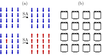
Figure 1: (a) The idealized spin amplification (SA) operation. If all spins are in the ground state initially, there is no change (top). If one spin is excited initially, all spins become excited (bottom). We consider an equal superposition of all the single excitation states instead of a particular excited spin position as shown in the figure. (b) The considered experimental platform: a 2D array of persistent-current artificial atoms [26] as the spin ensemble. The artificial atoms consist of a superconducting loops interrupted by $3$ Josephson junctions (crosses) where one of the junctions is smaller than the other two. The superconducting loops have linear inductance (inductors at the bottom of the loops), and the interactions between the spins are due the mutual inductance between the loops. The interactions are all-to-all in nature.

The transverse-field Ising model can be implemented on general-purpose quantum computers [4], but this requires individual drives for the spins. In contrast, ensembles of Rydberg atoms for instance, implement this model while utilizing a global drive [2, 3]. An implementation of the transverse-field Ising model can also be achieved by the ensembles of superconducting persistent-current artificial atoms [26, 27], which is what we focus on in the following. Compared to other superconducting artificial atoms with much better coherence properties [28, 29, 30], the primary advantage of the persistent-current artificial atoms is the small size that permits fabrication of thousands of spins on a compact chip [31]. Their large anharmonicity makes it possible to treat them as two-level systems even with strong drives, although large anharmonicities could also be obtained with for instance fluxonium [30] at the cost of a larger footprint. Due to being related to the persistent-current artificial atom, fluxonium can also have native $ZZ$-interactions [32]. This allows a fluxonium ensemble to be another possible implementation of the transverse-field Ising model.

Realistic spin systems have imperfections, such as long-range interactions, finite lifetimes, and inhomogeneous broadening [31, 2, 3, 33]. The position of the initial single excitation could be delocalized over the entire ensemble due to spins collectively absorbing a photon [34, 35]. Designing a protocol to amplify such delocalized states using imperfect spins is difficult to do manually. Therefore, we turn to optimal control [36] to replace the weak continuous-wave drive field with a time-dependent one that could be much stronger at its maximum.

The rest of the article is organized as follows. Our theoretical model and parameters are described in Sec. II with the results are presented in Sec. III. The implications of the results are discussed in Sec. IV with a conclusion also provided.

II Setup

We focus on the 2D layout of the spins (depicted schematically in Fig. 1(b)) due to it being easily transferrable to the experiments [31]. The spins are encoded in persistent-current artificial atoms, and the Hamiltonian of the ensemble is

$$\begin{gathered}H=-\hbar\sum_{j}\left(\frac{\Delta_{j}}{2}\hat{\sigma}_{z,j}+\Omega\hat{\sigma}_{+,j}+\Omega^{*}\hat{\sigma}_{-,j}\right)\\ +\hbar\sum_{\begin{subarray}{c}j,k\\ j\neq k\end{subarray}}J_{z,jk}\hat{\sigma}_{z,j}\hat{\sigma}_{z,k}+\hbar\sum_{\begin{subarray}{c}j,k\\ j\neq k\end{subarray}}J_{\pm,jk}\hat{\sigma}_{+,j}\hat{\sigma}_{-,k},\end{gathered}$$ (3)

where $\hat{\sigma}_{z,j}$ is the Pauli-$Z$ operator, $\hat{\sigma}_{\pm,j}$ is the raising/lowering operator, $\Delta_{j}=\omega_{\text{d}}-\omega_{01,j}$ is the detuning between the transition frequency $\omega_{01,j}$ for each spin $j$ and the carrier frequency of the drive $\omega_{\text{d}}$. The detunings can be written $\Delta_{j}=\Delta_{\text{avg}}+\omega_{{01},\text{avg}}-\omega_{01,j}$, where $\omega_{01,\text{avg}}$ is the average frequency (with averaging both over the spins in the ensemble and inhomogeneity realizations of the ensemble), and $\Delta_{\text{avg}}=\omega_{\text{d}}-\omega_{{01},\text{avg}}$. The Rabi frequency $\Omega$ can be time-dependent. The Hamiltonian is in the interaction picture with respect to $\omega_{\text{d}}$ and uses the rotating wave approximation. The transverse-field Ising model of Refs. [17, 19] is obtained when couplings are such that $J_{\pm,jk}=0$, and only the nearest-neighbor $J_{z,jk}$ are non-zero. We do not make such assumptions, and have $J_{z,jk},J_{\pm,jk}>0$ for all $j$ and $k$.

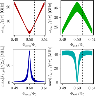
Figure 2: The parameters of the Hamiltonian (3) for the persistent-current artificial atoms [26] as spins: the transition frequencies between the ground and excited state $\omega_{01,j}$, the transition frequencies between the first and second excited states $\omega_{12,j}$, and the maximal (nearest-neighbor) values of the coupling strengths $J_{\pm,jk}$ and $J_{z,jk}$. Values for a range of bias fluxes $\Phi_{\text{ext}}/\Phi_{0}$ are shown, where $\Phi_{0}$ is the magnetic flux quantum. The curves are calculated by performing circuit quantization of the persistent-current artificial atoms with the Josephson junction area error of $2\%$ for $10^{4}$ different realizations of a square $4\times 4$ ensemble. The difference in the shown values between using $3\times 3$ and $4\times 4$ ensembles for averaging is small. The thickness of the curves shows the standard deviation of the parameters. To minimize the standard deviation of $\omega_{01,j}$, we choose a particular $\Phi_{\text{ext}}/\Phi_{0}=0.5034$ shown by the black dotted vertical line. The parameters of the persistent-current artificial atoms are close to Ref. [37]: $E_{J}/h=300\text{ GHz}$, $E_{J}/E_{C}=75$, $\alpha=0.7$ (relative area of the smaller junction). The model is extended to include the linear inductance, and the persistent-current artificial atoms are assumed to be square loops of size $3\text{ }\mu\text{m}\times 3\text{ }\mu\text{m}$ and use $0.2\text{ }\mu\text{m}\times 0.1\text{ }\mu\text{m}$ traces (width$\times$ height). The loops are spaced $1\text{ }\mu\text{m}$ apart.

Non-negligible $J_{\pm,jk}$ is caused by choosing the flux bias $\Phi_{\text{ext}}=0.5034\cdot\Phi_{0}$ for the persistent-current artificial atoms, where $\Phi_{0}$ is the magnetic flux quantum, that minimizes the inhomogeneous broadening [37]. This is illustrated in Fig. 2, where the parameters were calculated using circuit quantization [cf. App. A] with the Josephson junction area error of $2\%$ [38], and the other parameters are stated in the caption of the figure. For $\Phi_{\text{ext}}=0.5034\cdot\Phi_{0}$, we have the following parameters: the transition frequency between the ground state and the first excited state is $\omega_{01,j}/(2\pi)=7.9\pm 0.1\text{ GHz}$, the transition frequency between the first and second excited states is $\omega_{12,j}/(2\pi)=32.2\pm 2.1\text{ GHz}$, the maximal couplings $\text{max}|J_{\pm,jk}|/(2\pi)=5.7\pm 2.9\text{ MHz}$ and $\text{max}|J_{z,jk}|/(2\pi)=40.1\pm 4.0\text{ MHz}$. The transition frequency $\omega_{12,j}$ is only calculated to show that the anharmonicity is so large that the artificial atoms can be treated as two-level systems, and is not used in the Hamiltonian (3). Only the maximal couplings $|J_{\pm,jk}|$ and $|J_{z,jk}|$ are shown Fig. 2, which are the nearest-neighbor values, but coupling strengths for all $j$ and $k$ are calculated based on the mutual inductance between the superconducting loops and then used in the simulations. While performing circuit quantization, small additional inhomogeneous broadening of $\Delta_{j}$ appears due to the long-range couplings, even in the absence of fabrication imperfections.

We consider two different initial states: the zero-excitation state

$$|\psi_{0}\rangle=\bigotimes_{j}|0_{j}\rangle,$$ (4)

and the superposition of the single-excitation states

$$|\psi_{1}\rangle=\frac{1}{\sqrt{N}}\sum_{j}\hat{\sigma}_{+,j}|\psi_{0}\rangle$$ (5)

that could be a result of spins collectively absorbing a photon [34, 35]. The measurement operator for the population (total number) of the excited spins is $\hat{M}=\sum_{j}\hat{\sigma}_{+,j}\hat{\sigma}_{-,j}$. Writing the spin amplification operation as a superoperator $\mathcal{U}$, we thus maximize the expectation value

$$P_{1}-P_{0}=\operatorname{tr}[\hat{M}\mathcal{U}(|\psi_{1}\rangle\langle\psi_{1}|)]-\operatorname{tr}[\hat{M}\mathcal{U}(|\psi_{0}\rangle\langle\psi_{0}|)].$$ (6)

For the optimal control, one of the parametrizations of the Rabi frequency $\Omega$ in the Hamiltonian (3) is the Fourier series [39]

$$\text{Re}[\Omega](t)=\sqrt{\frac{2}{t_{\text{f}}}}\sum_{p=1}^{N_{\text{c}}}a_{p}\sin(\omega_{p}t),$$ (7a)

$$\text{Im}[\Omega](t)=\sqrt{\frac{2}{t_{\text{f}}}}\sum_{p=1}^{N_{\text{c}}}b_{p}\sin(\omega_{p}t),$$ (7b)

where $N_{\text{c}}$ is the number of the Fourier components, and $\omega_{p}=p\pi/t_{\text{f}}$. The Rabi frequency is zero for the initial time $t=0$ and the final time $t=t_{\text{f}}$. We set $N_{\text{c}}=100$ so that it is large enough to parametrize pulses with bandwidth of several GHz for amplification times below $10$ ns.

The parametrization (7) is only used to check the theoretical bounds, as it does not prevent the instantaneous amplitude of the Rabi frequency from becoming arbitrarily large. While it is possible to apply a nonlinear function, such as $\tanh$, to the right hand sides of Eqs. (7) to constrain the extremal values, this requires additional filtering (applying $\tanh$ increases the bandwidth) and defeats the purpose of limiting the bandwidth by truncating the Fourier series. We found it easier to constrain both the bandwidth and extremal values with the filtered piecewise-constant parametrization [40]. There, applying tanh to the coefficients suffices, resulting in

$$\begin{aligned} \text{Re}[\Omega_{\text{constrained}}](t)=\frac{\Omega_{\text{max}}}{\sqrt{2\pi}\sigma}\int_{-\infty}^{\infty}\exp\mathopen{}\left(-\frac{(t-t^{\prime})^{2}}{2\sigma^{2}}\right)\\ \times\sum_{p=1}^{N_{\text{c}}}\text{tanh}(a_{p})\mathbf{1}_{[(t_{\text{f}}/N_{\text{c}})(p-1),(t_{\text{f}}/N_{\text{c}})p]}(t^{\prime})\operatorname{d\!}t^{\prime},\end{aligned}$$ (8a)

$$\begin{aligned} \text{Im}[\Omega_{\text{constrained}}](t)=\frac{\Omega_{\text{max}}}{\sqrt{2\pi}\sigma}\int_{-\infty}^{\infty}\exp\mathopen{}\left(-\frac{(t-t^{\prime})^{2}}{2\sigma^{2}}\right)\\ \times\sum_{p=1}^{N_{\text{c}}}\text{tanh}(b_{p})\mathbf{1}_{[(t_{\text{f}}/N_{\text{c}})(p-1),(t_{\text{f}}/N_{\text{c}})p]}(t^{\prime})\operatorname{d\!}t^{\prime},\end{aligned}$$ (8b)

where $\Omega_{\text{max}}$ is the maximum Rabi frequency, and $\mathbf{1}_{[a,b]}$ is the indicator function defined as

$$\mathbf{1}_{[a,b]}(t)=\begin{cases}1~{}&\text{ if }t\in[a,b],\\ 0~{}&\text{ if }t\notin[a,b].\end{cases}$$ (9)

The integrals in Eqs. (8) can be evaluated analytically in terms of the error functions [40]. We assume the sampling rate of $10$ GS/s [41] (that determines $N_{\text{c}}$ in Eqs. (8)), and $1/\sigma=4\text{ GHz}$. To ensure that $\Omega_{\text{constrained}}$ is close to zero for $t=0$ and $t=t_{\text{f}}$, we set $a_{p}=0$ and $b_{p}=0$ with $p-1$ below $4\sigma N_{\text{c}}/t_{\text{f}}+1$ and above $N_{\text{c}}-4\sigma N_{\text{c}}/t_{\text{f}}-1$. This results in $|\Omega_{\text{constrained}}|<1$ kHz for $t=0$ and $t=t_{\text{f}}$ in the plots below.

The initial states are propagated in time with either the Schrödinger or master equation using the 4th order Runge-Kutta method. Ensembles with $N=16$ spins in the continuous-wave spin amplification are simulated using the quantum trajectory method [42], as it is faster than evolving the master equation. In all cases, the full Hilbert space with the basis size $2^{N}$ is used, necessitating significant computational power already for modestly large ensembles. We optimize the simulations by adopting a reduced-storage approach where only the states (state vectors or density matrices) are explicitly stored, while the operators and superoperators (the Hamiltonian and the dissipators of the master equation) are realized by calculating their action on the states [cf. App. B].

The detuning $\Delta_{\text{avg}}$ from the average spin frequency is optimized together with the pulse shape parameters $a_{p}$ and $b_{p}$. Our optimal control approach is similar to Ref. [43], where the gradient of the final population difference (6) with respect to the pulse parameters is found using the reverse-mode automatic differentiation [cf. App. C] and then used in a gradient-based optimization algorithm LBFGS [44]. In our implementation, the total memory requirements for the optimal control are around $14.5$ ($18.5$) times the size of the density matrix (state vector). The difference between the multiples for the density matrix and the state vector, is that some auxiliary vectors have a fixed size equal to the state vector, and hence are negligible in size compared to the density matrix. Importantly, the memory requirements are independent of the number of the optimal control parameters and simulation time steps. The latter is achieved by propagating the states backward in time during the gradient calculation [45, 46]. This makes it possible to simulate and optimize the control pulse shapes for ensembles of up to $N=16$ spins.

Since the persistent-current artificial atoms are operated away from the degeneracy point, their coherence is expected to be limited. We assume pure dephasing time $T_{\phi}=100\text{ }\text{ns}$ and decay time $T_{1}=1\text{ }\mu\text{s}$ [47]. To perform the spin amplification approximately coherently, the amplification time needs to be chosen much smaller than $T_{\phi}$, and we set it to be $t_{\text{f}}=6.5\text{ ns}$. This is close to the time scale set by the interaction $1/\text{max}|J_{z,jk}|\approx 4\text{ ns}$. This is in contrast with the previous spin amplification protocols [17, 18, 19] that used a small constant Rabi frequency $|\Omega|\ll\text{max}|J_{z,jk}|$ that resulted in amplification times much longer than $1/\text{max}|J_{z,jk}|$. This approach only works for long $T_{1}$ and $T_{\phi}$. Finite $T_{\phi}$ makes the spin amplification slower [19] and also introduces erroneous excitations in the initial zero-excitation case as explained in App. D. Finite $T_{1}$ limits the total achievable excitation number in the single-excitation case. While choosing a larger $|\Omega|$ could partially compensate for this, this also increases the zero-excitation error due to the finite $T_{\phi}$.

III Results

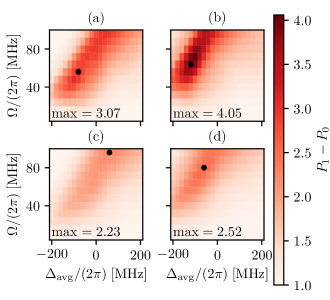
Figure 3: Maximal difference of the populations $P_{1}-P_{0}$ within a time window of $6.5$ ns for the continuous-wave spin amplification as a function of the Rabi frequency $\Omega$ and the detuning $\Delta_{\text{d}}$ of the drive from the average spin frequency. The overall maximum for the considered range of $\Omega$ and $\Delta_{\text{d}}$ is written in the bottom left corner of each subplot. The black dots show the parameters for which the maxima are obtained. (a) $N=9$ spins without inhomogeneity, (b) $N=16$ without inhomogeneity, (c) $N=9$ with inhomogeneity, (d) $N=16$ with inhomogeneity. For $N=9$, the master equation is used, while $N=16$ is calculated using the quantum trajectory method with $500$ trajectories. The influence of the inhomogeneity is evaluated in the $N=9$ case by propagating the master equation $100$ times with different ensemble realizations, and averaging the results. In the $N=16$ case, the averaging over the inhomogeneity and the different quantum trajectories of the decay and dephasing is done simultaneously for efficiency. Therefore, a different inhomogeneity realization is chosen for every trajectory.

To show that optimal control pulses are needed for the considered system, we first show the performance of the continuous-wave spin amplification in Fig. 3. The maximal achievable population differences $P_{1}-P_{0}$ are calculated for different Rabi frequencies $\Omega$ and detunings $\Delta_{\text{avg}}=\omega_{\text{d}}-\omega_{01,\text{avg}}$ from the average spin frequency. The amplification time is chosen such that $P_{1}-P_{0}$ is maximal within the first $6.5$ ns after the drive is applied. The simulations without inhomogeneity use the average values of $\Delta_{j}$, $J_{\pm,jk}$, and $J_{z,jk}$ in the Hamiltonian (3) that were calculated as if the Josephson junction area error were $2\%$, but without including the variations due to different inhomogeneity realizations. This is done to match more closely the average values between the inhomogeneous and homogeneous cases. The averaging is not done over the different couplings within the ensemble, so that the more distant spins still have weaker couplings compared to the the nearest neighbors. Choosing the optimal $\Omega$ and $\Delta_{\text{avg}}$, $P_{1}-P_{0}=3.07$ is achieved for $N=9$ and $P_{1}-P_{0}=4.05$ is achieved for $N=16$. Inhomogeneity reduces the maximal population differences to $P_{1}-P_{0}=2.23$ for $N=9$ and $P_{1}-P_{0}=2.52$ for $N=16$. In all cases, the optimal $\Omega/(2\pi)$ is larger than $\text{max}|J_{z,jk}|/(2\pi)\approx 40$ MHz, and hence outside of the parameter regime that was considered in Refs. [17, 18, 19].

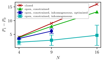
Figure 4: Difference of the final populations $P_{1}-P_{0}$ for the spin amplification with time-dependent drives found using optimal control as a function of the number of spins $N$. The closed system results using the pulse parametrization (7) (red crosses) lie very close to the line $P_{1}-P_{0}=N$. For the open systems, the constrained parametrization (8) is used. The pulse shapes for the inhomogeneous open systems are either optimized (blue circles) or taken to be the same (cyan squares) as the corresponding homogeneous open systems (green triangles). The inhomogeneity is modeled by averaging over $100$ realizations, and the error bars show the standard deviation of this averaging.

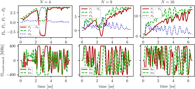
Figure 5: Populations as functions of time for the open system without inhomogeneity (top) and pulse shapes (bottom) for the different ensemble sizes $N=4,9,16$. The final $P_{1}-P_{0}$ values correspond to the green triangles in Fig. 4. Pulse shapes are parametrized such that the extremal values of $\text{Re}[\Omega_{\text{constrained}}]$ and $\text{Im}[\Omega_{\text{constrained}}]$ [cf. Eqs. (8)] are at $\pm 400$ MHz, and the filtering bandwidth is $1/\sigma=4\text{ GHz}$.

We also evaluate the performance of a two-frequency continuous-wave drive [19]. The Rabi frequency becomes time-dependent with the parametrization

$$\Omega(t)=\Omega_{1}+\Omega_{2}\exp(i(\Delta_{\text{avg},1}-\Delta_{\text{avg},2})t),$$ (10)

where the detuning $\Delta_{\text{avg},1}=\omega_{\text{d},1}-\omega_{01,\text{avg}}$ of the first frequency component is included in $\Delta_{j}=\Delta_{\text{avg},1}+\omega_{{01},\text{avg}}-\omega_{01,j}$ in the Hamiltonian (3). A global optimization with the algorithm DIRECT [48, 49] over $\Omega_{l}$ and $\Delta_{\text{avg},l}$ for $l=1,2$ inside the bounds $\Omega_{l}\in[0.1,2.4]\cdot 40\text{MHz}$, $\Delta_{\text{avg},l}\in[-5,5]\cdot 40\text{MHz}$ (where $40\text{MHz}\approx\text{max}|J_{z,jk}|/(2\pi)$) did not yield much improvement over the single-frequency case. For $N=9$ without inhomogeneity, $P_{1}-P_{0}=3.19$ is obtained, and for $N=16$, $P_{1}-P_{0}=4.10$ is obtained. Having verified that even a two-frequency continuous-wave drive is insufficient to reach good spin amplification performance, we proceed to explore a more general broadband drive with an optimal control algorithm to find the pulse shape.

The overview of the results of the optimally-controlled spin amplification is shown in Fig. 4 as a function of the number of spins $N$. In all cases, the pulse shapes are initialized randomly with $\Delta_{\text{avg}}/(40\text{ MHz})$ and each $a_{p}$ and $b_{p}$ sampled from the standard normal distribution (with mean $0$ and standard deviation $1$). We take $10$ such realizations and pick the best optimized pulse shape as the result. This is done because the optimization has a tendency to converge to the local optima.

To establish a baseline, we perform the calculations using the pulse shape parametrization (7) in a closed system without the decay and dephasing ($T_{1}\rightarrow\infty$ and $T_{\phi}\rightarrow\infty$) and without inhomogeneity. The long-range interactions are still fully accounted for. These results (red crosses) lie very close to the line $P_{1}-P_{0}=N$ and show that it is in principle possible to saturate the bound set by the maximal number of spins. For the open system results (green triangles), the constrained parametrization (8) is used. The constrained pulses were optimized for the closed system first, and then the optimal pulse shapes were used as the initial values for the open system optimizations. This significantly reduces the optimization time for $N=16$. In this case, a single iteration for the open system takes around $86$ hours while running on $2$ cluster nodes, each having dual AMD Epyc 7702 CPUs ($128$ cores in total). The nodes calculate the values and gradients of $P_{0}$ and $P_{1}$ in parallel. The optimized pulse shapes are shown in Fig. 5.

Optimizing the pulse shapes for the inhomogeneous ensembles is slow due to having to evaluate many realizations at each iteration. This is why we only go up to $N=9$ (blue circles). We found that it is better to optimize the inhomogeneous case from scratch instead of starting with the optimal pulse shapes from the homogeneous ensemble. The optimized pulse shapes for $N=9$ are shown in Fig. 6. To see the trend up to $N=16$ for the inhomogeneous ensembles, the pulse shapes for the homogeneous ensembles are used without further optimization (cyan squares). The performance is significantly decreased (lower average $P_{1}-P_{0}$ and larger standard deviation) compared to the case where the pulses were optimized for the inhomogeneity, but the total population difference is still seen to increase with the ensemble size. Thus, a similar trend is expected for the inhomogeneous ensemble with $N=16$ driven by optimized pulse shapes, but with a larger average value $P_{1}-P_{0}$ and smaller standard deviation.

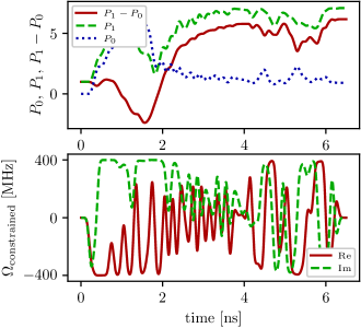
Figure 6: Average populations as functions of time for the open system with inhomogeneity (top) and optimized pulse shapes (bottom) for $N=9$ spins.

IV Discussion and conclusion

Spin amplification is both useful in itself for quantum sensing or measurement, and as a step on the way to the universal quantum computation with a global driving field. For the quantum measurement of a single spin excitation with a global drive, spin amplification could be used before the global excitation is measured. In the above, we have considered persistent-current artificial atoms operated away from the degeneracy point as spins. In this case, the two spin states are associated with different magnetic fields that can be distinguished by a magnetometer. A superconducting quantum interference device (SQUID) fabricated on the same chip such that it encloses the entire ensemble, could be used as such a magnetometer [50]. The single excitation that is amplified could be a result of an absorption of a single photon. In this case, spin amplification can be viewed as having the same function as the internal dynamics of the single-photon avalanche detectors [51].

Universal quantum computation with globally driven spin ensembles is also possible [13, 14, 16, 21, 22]. The techniques that we have developed for the analysis of spin amplification, could be used to better understand which other operations can be performed with such setups even in the presence of imperfections.

It is possible to have ensembles with much larger numbers of spins [2, 3, 31] than we have considered. To find pulse shapes for such ensembles theoretically, the direct simulation of the exponentially-large Hilbert space is impossible. Alternative approaches, such as the matrix-product states [2, 3, 52] or semiclassical methods [52], will be required. Experimentally, the pulses could also be found by optimizing the setup directly [53].

To conclude, our calculations show that spin amplification is possible in noisy spin ensemble consisting of superconducting persistent-current artificial atoms. This is done by employing optimal control techniques to find classical drive pulse shapes. Thereby the time of the spin amplification is significantly shortened compared to the previous protocols that use weak continuous-wave drives. We expect that using the same approach will make it possible to implement spin amplification in other kinds of spins, such as the Rydberg atoms.

Appendix A Persistent-current artificial atoms

In this appendix, we show how the spin Hamiltonian (3) can be derived from the circuit quantization of the persistent-current artificial atoms [26]. We need to include the self-inductance terms in the artificial atom Hamiltonian [54, 55, 56, 57], because they significantly modify the transition frequencies and are needed to introduce the couplings that are caused by the mutual inductance. The inductance matrix $\mathbf{L}$ that combines both the self-inductances (diagonal elements) and the mutual inductances (off-diagonal elements) is calculated using a version of FASTHENRY [58] that includes the kinetic inductance due to superconductivity [59]. For the calculation of the kinetic inductance, we set the London penetration depth $\lambda=0.2\text{ }\mu\text{m}$ as an order-of-magnitude estimate, in line with the measurements of the aluminum thin films [60]. For our parameters [see caption of Fig. 2], we get self-inductance $L=37.4$ pH, and the mutual inductance of the nearest neighbors $M=-0.2$ pH.

Before the Hamiltonian can be found, a classical Lagrangian $\mathcal{L}_{j}$ for the persistent-current artificial atom $j$ is determined from the flux variables shown in Fig. 7. The index $j$ is omitted on the flux variables for brevity. The fluxes are time integrals of voltages $\Phi_{C}(t)=\int_{-\infty}^{t}V_{C}(t^{\prime})\operatorname{d\!}t^{\prime}$, and the voltages are electric field line integrals $V_{C}=\int_{C}\vec{E}\cdot\operatorname{d\!}\vec{l}$ [61, 62] along the different contours $C$ that are segments of the loop, as shown in Fig. 7. There is gauge freedom [61, 62] in the sense that different choices of the contours $C$ are possible [55, 56, 57], but they all lead to the same quantum energy levels. The total inductive energy in the ensemble is $\vec{\Phi}_{L}^{\text{T}}\mathbf{L}^{-1}\vec{\Phi}_{L}$ [62], where $\vec{\Phi}_{L}$ is a vector with $N$ elements for the fluxes that correspond to the linear inductance in each artificial atom, and $\mathbf{L}^{-1}$ is the inverse of the inductance matrix. We include the diagonal terms of this expression that are proportional to $(\mathbf{L}^{-1})_{jj}$ in the potential energies of each artificial atom. The off-diagonal terms are subsequently projected onto the eigenstates to give the couplings between the artificial atoms.

We have $\mathcal{L}_{j}=T_{j}-U_{j}$, where the kinetic energy is

$$T_{j}=\frac{\alpha_{1}C_{\text{J}}}{2}\left(\dot{\Phi}_{1}-\dot{\Phi}_{2}\right)^{2}+\frac{\alpha_{2}C_{\text{J}}}{2}\left(\dot{\Phi}_{2}-\dot{\Phi}_{3}\right)^{2}+\frac{\alpha_{3}C_{\text{J}}}{2}\dot{\Phi}_{3}^{2},$$ (11)

the potential energy is

$$\begin{aligned} &U_{j}=(\mathbf{L}^{-1})_{jj}\frac{\Phi_{L}^{2}}{2}-\alpha_{1}E_{\text{J}}\cos\left(\frac{2\pi}{\Phi_{0}}(\Phi_{1}-\Phi_{2})\right)\\ &-\alpha_{2}E_{J}\cos\left(\frac{2\pi}{\Phi_{0}}(\Phi_{2}-\Phi_{3})\right)-\alpha_{3}E_{J}\cos\left(\frac{2\pi}{\Phi_{0}}\Phi_{3}\right),\end{aligned}$$ (12)

and ${\Phi_{0}=h/(2e)\approx 2.068\times 10^{-15}}$ Wb is the magnetic flux quantum. The Josephson junction energies $E_{J}$ and capacitances $C_{J}$ are proportional to the Josephson junction area and are scaled by the dimensionless parameters $\alpha_{l}$. In the ideal case, $\alpha_{1}=\alpha_{3}=1$ and $\alpha_{2}=\alpha=0.7$, but due to fabrication imperfections the actual values deviate from the ideal ones. For the calculations with inhomogeneity, the values of $\alpha_{l}$ are sampled from a Gaussian distribution with the average value $\mu$ equal to the ideal one, and the standard deviation $\sigma=0.02$.

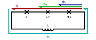
Figure 7: Flux variable definitions. The integration contours that correspond to the flux variables are displaced out of the circuit for clarity, since some of them overlap.

The flux variables are not independent, as there is a constraint on the total flux through the loop given by

$$\Phi_{\text{ext}}=\int_{-\infty}^{t}\oint\vec{E}(t^{\prime})\cdot\operatorname{d\!}\vec{l}\operatorname{d\!}t^{\prime}=\Phi_{1}+\Phi_{L}.$$ (13)

The flux variable $\Phi_{1}$ can be eliminated using the constraint above. Assuming external flux that is constant in time, $\dot{\Phi}_{\text{ext}}=0$, the kinetic energy is

$$T_{j}=\frac{\alpha_{1}C_{\text{J}}}{2}\left(\dot{\Phi}_{L}+\dot{\Phi}_{2}\right)^{2}+\frac{\alpha_{2}C_{\text{J}}}{2}\left(\dot{\Phi}_{2}-\dot{\Phi}_{3}\right)^{2}+\frac{\alpha_{3}C_{\text{J}}}{2}\dot{\Phi}_{3}^{2},$$ (14)

and the potential energy is

$$\begin{aligned} &U_{j}=(\mathbf{L}^{-1})_{jj}\frac{\Phi_{L}^{2}}{2}-\alpha_{1}E_{\text{J}}\cos\left(\frac{2\pi}{\Phi_{0}}(\Phi_{\text{ext}}-\Phi_{L}-\Phi_{2})\right)\\ &-\alpha_{2}E_{J}\cos\left(\frac{2\pi}{\Phi_{0}}(\Phi_{2}-\Phi_{3})\right)-\alpha_{3}E_{J}\cos\left(\frac{2\pi}{\Phi_{0}}\Phi_{3}\right).\end{aligned}$$ (15)

The kinetic energy can be written in terms of the capacitance matrix

$$\hat{C}=C_{J}\begin{pmatrix}\alpha_{2}+\alpha_{3}&-\alpha_{2}&\alpha_{1}\\ -\alpha_{2}&\alpha_{1}+\alpha_{2}&0\\ \alpha_{1}&0&\alpha_{1}\end{pmatrix}$$ (16)

as $T_{j}=(1/2)\dot{\vec{\Phi}}^{\text{T}}\hat{C}\dot{\vec{\Phi}}$, where $\vec{\Phi}^{\text{T}}=(\Phi_{2},\Phi_{3},\Phi_{L})$ is the transpose of $\vec{\Phi}$.

The next step is to perform the Legendre transformation and thereby find the classical Hamiltonian. For the Legendre transformation, the vector of the canonical momenta is determined as

$$\vec{Q}=\dfrac{\partial{}L}{\partial{\dot{\vec{\Phi}}}}=\hat{C}\dot{\vec{\Phi}}.$$ (17)

The classical Hamiltonian is then

$$H_{j}=\vec{Q}^{\text{T}}\dot{\vec{\Phi}}-\mathcal{L}_{j}=2T_{j}-\mathcal{L}_{j}=T_{j}+U_{j},$$ (18)

where the kinetic energy written in terms of the canonical momenta is $T_{j}=(1/2)\vec{Q}^{\text{T}}\hat{C}^{-1}\vec{Q}$.

Performing the canonical quantization, the Poisson bracket $\{\Phi_{l},Q_{m}\}=\delta_{l,m}$ is replaced with the commutator $[\hat{\Phi}_{l},\hat{Q}_{m}]=i\hbar\delta_{l,m}$. Defining the dimensionless external flux $f=\Phi_{\text{ext}}/\Phi_{0}$ and operators

$$\hat{n}_{l}=\frac{1}{2e}\hat{Q}_{l}, \hat{\varphi}_{l}=\frac{2\pi}{\Phi_{0}}\hat{\Phi}_{l},$$ (19)

with the commutator $[\hat{\varphi}_{l},\hat{n}_{m}]=i\delta_{l,m}$, the kinetic energy can be written $\hat{T}_{j}=4E_{C}\vec{n}^{\text{T}}\hat{C}^{-1}\vec{n}$ with $E_{C}=e^{2}/(2C_{J})$. The Hamiltonian is

$$\begin{aligned} \hat{H}_{j}=&\;\hat{T}_{j}+\frac{1}{2}E_{L}\hat{\varphi}_{L}^{2}-\alpha_{1}E_{\text{J}}\cos\left(2\pi f-\hat{\varphi}_{L}-\hat{\varphi}_{2}\right)\\ &-\alpha_{2}E_{J}\cos\left(\hat{\varphi}_{2}-\hat{\varphi}_{3}\right)-\alpha_{3}E_{J}\cos\left(\hat{\varphi}_{3}\right),\end{aligned}$$ (20)

where $E_{L}=(\mathbf{L}^{-1})_{jj}(\Phi_{0}/(2\pi))^{2}$.

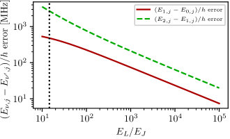
Figure 8: The error in calculating the transition frequencies $(E_{1,j}-E_{0,j})/h$ and $(E_{2,j}-E_{1,j})/h$ for a persistent-current artificial atom $j$ using the zero-self-inductance Hamiltonian (21), compared to the Hamiltonian (20) that accounts for the finite self-inductance. The error is plotted as a function of the ratio of the inductive energy $E_{L}$ and Josephson energy $E_{J}$. For the the Hamiltonian (20), the ideal values $\alpha_{1}=\alpha_{3}=1$ and $\alpha_{2}=\alpha$ are used. The bias flux is $f=\Phi_{\text{ext}}/\Phi_{0}=0.5034$ in both cases. Other parameters are stated in the caption of Fig. 2, but the Josephson junction area error is not included. Assuming that the artificial atom is isolated, i.e., the inductance matrix $\mathbf{L}$ has only one element $L=37.4$ pH, we have $E_{L}/E_{J}=14.5$, which is shown by the black dotted vertical line.

In the limit $L\rightarrow 0$ ($E_{L}\rightarrow\infty$), the constraint $\hat{\varphi}_{L}=0$ is imposed. Replacing $\hat{\varphi}_{2}\rightarrow\hat{\varphi}_{2}-\hat{\varphi}_{1}$ and $\hat{\varphi}_{3}\rightarrow-\hat{\varphi}_{1}$, and using the ideal $\alpha_{1}=\alpha_{3}=1$ and $\alpha_{2}=\alpha$, the Hamiltonian reduces to the one considered in Ref. [26]:

$$\begin{aligned} \hat{H}_{j,0}=&\;T_{j,0}-\big{(}E_{J}\cos(\hat{\varphi}_{1})+E_{J}\cos(\hat{\varphi}_{2})\\ &+\alpha E_{J}\cos(2\pi f+\hat{\varphi}_{1}-\hat{\varphi}_{2})\big{)}.\end{aligned}$$ (21)

The end result of the Hamiltonian diagonalization can be written as $\hat{H}_{j}=\sum_{\nu=0}^{\infty}E_{\nu,j}|\nu_{j}\rangle\langle\nu_{j}|$ in terms of the eigenenergies $E_{\nu,j}$ and the eigenvectors $|\nu_{j}\rangle$. For a finite $L$, there is a significant difference in the spectrum between the Hamiltonians $\hat{H}_{j,0}$ and $\hat{H}_{j}$, as shown in Fig. 8. Our parameters approximately correspond to $E_{L}/E_{J}=14.5$ (ignoring the mutual inductance), and for this value the Hamiltonian (20) gives $(E_{1,j}-E_{0,j})/h=7.9$ GHz, while the Hamiltonian (21) gives $(E_{1,j}-E_{0,j})/h=8.4$ GHz.

For the case of finite but small $L$ that we consider, the term $(1/2)E_{L}\hat{\varphi}_{L}^{2}$ is dominant in the Hamiltonian (20). To reduce the total number of the basis states required to diagonalize the entire Hamiltonian (20), a harmonic oscillator basis is chosen where the quadratic part

$$\hat{H}_{L}=A\hat{n}_{L}^{2}+B\hat{\varphi}_{L}^{2}$$ (22)

is already diagonal. In Eq. (22), $A$ is proportional to the element of the inverse capacitance matrix $\hat{C}^{-1}$ corresponding to $\hat{\varphi}_{L}$, and $B=(1/2)E_{L}$. The operators are written $\hat{\varphi}_{L}=\frac{1}{C_{L}}\frac{1}{\sqrt{2}}(\hat{a}+\hat{a}^{\dagger})$, and $\hat{n}_{L}=-iC_{L}\frac{1}{\sqrt{2}}(\hat{a}-\hat{a}^{\dagger})$, where the creation operator $\hat{a}^{\dagger}$ and the annihilation operator $\hat{a}$ are defined by their actions on the Fock states $|n_{L}\rangle$. We have $\hat{a}^{\dagger}|n_{L}\rangle=\sqrt{n_{L}+1}|n_{L}+1\rangle$ and $\hat{a}|n_{L}\rangle=\sqrt{n_{L}}|n_{L}-1\rangle$. The commutator $[\hat{\varphi}_{L},\hat{n}_{L}]=i$ is satisfied for any choice of the constant $C_{L}$, but to diagonalize Eq. (22), a particular $C_{L}=(B/A)^{1/4}$ is chosen, resulting in $\hat{H}_{L}=2\sqrt{AB}\mathinner{\left(\hat{a}^{\dagger}\hat{a}+\frac{1}{2}\right)}$.

For the representation of the Josephson-junction operators in (phases $\hat{\varphi}_{2}$ and $\hat{\varphi}_{3}$, and the corresponding charge numbers $\hat{n}_{2}$ and $\hat{n}_{3}$ in Eq. (20)), the charge basis is used. In this basis, the eigenstates are $|n_{l}\rangle$ where $l=2,3$; and the operators can be written $\hat{n}_{l}=\sum_{n_{l}=-\infty}^{\infty}n_{l}|n_{l}\rangle\langle n_{l}|$, and $e^{-i\hat{\varphi}_{l}}=\sum_{n_{l}=-\infty}^{\infty}|n_{l}\rangle\langle n_{l}-1|$. In the harmonic oscillator basis, $e^{-i\hat{\varphi}_{L}}$ is computed using matrix exponentiation. The Hilbert spaces of the Josephson junctions are truncated to $21$ charge states each, and the harmonic oscillator basis to $8$ Fock states.

For the numerical diagonalization of Eq. (20), the matrix exponentials are decomposed using tensor products. E.g., the expression $e^{i\hat{\varphi}_{2}-i\hat{\varphi}_{3}}$ in Eq. (20) is actually

$$\begin{aligned} &\exp\mathopen{}\mathinner{\left(i\hat{\varphi}_{2}\otimes\hat{I}_{3}\otimes\hat{I}_{L}-i\hat{I}_{2}\otimes\hat{\varphi}_{3}\otimes\hat{I}_{L}\right)}\\ &=\exp\mathopen{}\mathinner{\left(i\hat{\varphi}_{2}\right)}\otimes\exp\mathopen{}\mathinner{\left(-i\hat{\varphi}_{3}\right)}\otimes\hat{I}_{L}\end{aligned}$$ (23)

where $\hat{I}_{2}$, $\hat{I}_{3}$ and $\hat{I}_{L}$ are the identity operators on the respective Hilbert spaces. In Eq. (23), we have used the fact that $e^{\hat{A}+\hat{B}}=e^{\hat{A}}e^{\hat{B}}$ for commuting matrices $\hat{A}$ and $\hat{B}$, and that

$$\exp(\hat{A}\otimes\hat{I})=\exp(\hat{A})\otimes\hat{I}.$$

Similarly, the other operators in Eq. (20) are rewritten with the identity operators appearing explicitly. E.g., $\hat{Q}_{2}^{2}$ becomes $\hat{Q}_{2}^{2}\otimes\hat{I}_{3}\otimes\hat{I}_{L}$. It is the latter types of expressions that are used to assemble the matrix for the numerical diagonalization.

Coupling between the artificial atoms with Hamiltonians $\hat{H}_{j}$ is due to the off-diagonal elements of the inverse inductance matrix $\mathbf{L}^{-1}$. The Hamiltonian for the entire ensemble can be written

$$\hat{H}_{\text{ensemble}}=\sum_{j}\hat{H}_{j}+\sum_{\begin{subarray}{c}j,k\\ j\neq k\end{subarray}}(\mathbf{L}^{-1})_{jk}\hat{\Phi}_{L,j}\hat{\Phi}_{L,k}.$$ (24)

Making the two-level approximation, the operators $\hat{\Phi}_{L,j}$ are projected onto the subspace spanned by the eigenvectors $|0_{j}\rangle$ and $|1_{j}\rangle$ of $\hat{H}_{j}$ and hence can be written as the Hermitian $2\times 2$ matrices

$$\hat{\Phi}_{L,j}=\begin{pmatrix}\langle 0_{j}|\hat{\Phi}_{L,j}|0_{j}\rangle&\langle 0_{j}|\hat{\Phi}_{L,j}|1_{j}\rangle\\ \langle 1_{j}|\hat{\Phi}_{L,j}|0_{j}\rangle&\langle 1_{j}|\hat{\Phi}_{L,j}|1_{j}\rangle\end{pmatrix}.$$ (25)

Such matrices can be decomposed into linear combinations of Pauli matrices and the identity matrix $\hat{I}_{j}$. Thus,

$$\hat{\Phi}_{L,j}=P_{\hat{I}_{j}}+P_{\hat{\sigma}_{x,j}}\hat{\sigma}_{x,j}+P_{\hat{\sigma}_{y,j}}\hat{\sigma}_{y,j}+P_{\hat{\sigma}_{z,j}}\hat{\sigma}_{z,j},$$ (26)

where $P_{\hat{O}_{j}}$ for $\hat{O}_{j}\in\{\hat{I}_{j},\hat{\sigma}_{x,j},\hat{\sigma}_{y,j},\hat{\sigma}_{z,j}\}$ are real coefficients found via the Hilbert-Schmidt inner product

$$P_{\hat{O}_{j}}=\frac{1}{2}\text{tr}\left[\hat{\Phi}_{L,j}\hat{O}_{j}\right].$$ (27)

The eigenvectors are defined up to a phase, and the relative phases of the lowest-energy states $|0_{j}\rangle$ and $|1_{j}\rangle$ are chosen such that $\langle 0_{j}|\hat{\Phi}_{L,j}|1_{j}\rangle$ is real. This results in $P_{\hat{\sigma}_{y,j}}=0$, but we still keep it in the expressions for generality.

Inserting Eq. (26) into Eq. (24), applying the rotating wave approximation, and removing constants, we get

$$\begin{aligned} \hat{H}_{\text{ensemble}}&=\hbar\sum_{j}\frac{\omega_{j}}{2}\hat{\sigma}_{z,j}+\hbar\sum_{\begin{subarray}{c}j,k\\ j\neq k\end{subarray}}J_{z,jk}\hat{\sigma}_{z,j}\hat{\sigma}_{z,k}\\ &+\hbar\sum_{\begin{subarray}{c}j,k\\ j\neq k\end{subarray}}J_{\pm,jk}\hat{\sigma}_{+,j}\hat{\sigma}_{-,k}\end{aligned}$$ (28)

with

$$\omega_{j}=\frac{E_{1,j}-E_{0,j}}{\hbar}+4\sum_{\begin{subarray}{c}k\\ k\neq j\end{subarray}}\frac{(\mathbf{L}^{-1})_{jk}}{\hbar}P_{\hat{\sigma}_{z,j}}P_{\hat{I}_{k}},$$ (29)

$$J_{z,jk}=\frac{(\mathbf{L}^{-1})_{jk}}{\hbar}P_{\hat{\sigma}_{z,j}}P_{\hat{\sigma}_{z,k}},$$ (30)

$$J_{\pm,jk}=2\frac{(\mathbf{L}^{-1})_{jk}}{\hbar}(P_{\hat{\sigma}_{x,j}}-iP_{\hat{\sigma}_{y,j}})(P_{\hat{\sigma}_{x,k}}+iP_{\hat{\sigma}_{y,k}}).$$ (31)

The coupling $J_{\pm,jk}$ is real because of $P_{\hat{\sigma}_{y,j}}=0$. Adding the driving terms and going into the rotating frame with respect to $\hat{H}_{0}=(\hbar\omega_{\text{d}}/2)\sum_{j}\hat{\sigma}_{z,j}$ results in the Hamiltonian (3) of the main text. Note that Eq. (29) shows that even without fabrication imperfections, there is a small inhomogeneous broadening in the renormalized spin frequencies due to the fact that spins experience different sum of mutual inductances between them and the neighbors.

Appendix B Reduced-storage operators

In this appendix, we show how the action of the quantum mechanical operators and superoperators can be calculated with reduced storage requirements. The state vectors $\psi$ of the closed systems are propagated in time using the Schrödinger equation

$$\dot{\psi}=-\frac{i}{\hbar}\hat{H}\psi,$$ (32)

where the Hamiltonian $\hat{H}$ is given by Eq. (3), and the ket notation on the state vectors is omitted. The density matrices $\rho$ of the open systems are propagated in time using the Markovian zero-temperature master equation

$$\dot{\rho}=-\frac{i}{\hbar}[\hat{H},\rho]+\gamma\sum_{j}\mathcal{D}[\hat{\sigma}_{-,j}]\rho+\gamma_{\text{d}}\sum_{j}\mathcal{D}[\hat{\sigma}_{z,j}]\rho,$$ (33)

where $\mathcal{D}[\hat{o}]\rho=\frac{1}{2}(2\hat{o}\rho\hat{o}^{\dagger}-\rho\hat{o}^{\dagger}\hat{o}-\hat{o}^{\dagger}\hat{o}\rho)$.

For an ensemble of two-level systems, there is a direct mapping between binary numbers and basis states. The zero-excitation state $\psi_{0}$ [Eq. (4)] is mapped to the binary number $0$. A basis state $\hat{\sigma}_{+,j}\hat{\sigma}_{+,k}\psi_{0}$ that has spins $j$ and $k$ up and all other spins down, is mapped to the binary number where bits $j$ and $k$ are set (equal to $1$), and all the other bits are reset (equal to $0$). Interpreted as an integer, this number has value $2^{j}+2^{k}$ (if $j$ and $k$ are zero-based indices), but exponentiation is not needed to calculate it—only bitwise operations that directly set the corresponding bits. The amplitudes of the state vector $\psi$ are stored in an array with the positions corresponding to the binary numbers obtained by the above mapping. For the density matrix $\rho$, both the row and the column of an element are determined by this mapping. Thus, given a basis state specification (i.e., which spins are up and which are down), it allows to quickly determine the position of the corresponding state vector amplitude or density matrix element in the stored arrays. This leads to an efficient calculation of the action of operators both in the Schrödinger equation (32) and the master equation (33).

The commutator term on the right-hand side of master equation (33) can be written

$$-\frac{i}{\hbar}[\hat{H},\rho]=-\frac{i}{\hbar}\hat{H}\rho+\left(-\frac{i}{\hbar}\hat{H}\rho\right)^{\dagger},$$ (34)

where we have used the fact $\hat{H}$ and $\rho$ are Hermitian, i.e., $\hat{H}^{\dagger}=\hat{H}$ and $\rho^{\dagger}=\rho$. Writing the commutator term like this, shows that only $-\frac{i}{\hbar}\hat{H}\rho$ needs to be calculated by applying $-\frac{i}{\hbar}\hat{H}$ to each column of $\rho$ just like in a Schrödinger equation (32), and then the adjoint of the resulting matrix can be added to itself to obtain $-\frac{i}{\hbar}[\hat{H},\rho]$. Hence, we first need to be able to calculate the action of $\hat{H}$ on a state vector $\psi$.

The operators $-\sum_{j}\frac{\Delta_{j}}{2}\hat{\sigma}_{z,j}$ and $\sum_{j\neq k}J_{z,jk}\hat{\sigma}_{z,j}\hat{\sigma}_{z,k}$ in the Hamiltonian (3) are diagonal, and therefore their storage requirements are the same as for the state vector $\psi$ itself. Even though the action of these operators could be calculating on the fly, we find that storing the diagonal of the matrix and multiplying it onto $\psi$ is faster. It is possible, however, to adapt the below code that calculates the diagonal to immediately multiply each element with a corresponding element of a vector instead of storing it. Thereby the computation could be performed in a completely matrix-free way.

Operator	Description
<<	bitwise shift
&	bitwise AND
|	bitwise OR
~	bitwise NOT
&&	logical AND
||	logical OR
!	logical NOT

Table 1: Logical and bitwise operators used in the pseudo-code examples.

We will explain both this and the other computations in terms of the pseudo-code, where the bitwise and logical operators follow the conventions of C and C++ languages. The operators are listed in Table 1. The loops in the pseudo-code are written in terms of zero-based indices. E.g., n is an index of the basis for which it holds that $0\leq\verb+n+\leq 2^{N}-1$; and j,k are indices of the spins for which it holds that $0\leq\verb+j+,\verb+k+\leq N-1$. The basis size is written compactly using the bitwise shift operator as 1 << N, which is equal to $2^{N}$. The variables are set using =, so that n = n + 1 means that $1$ is added to n.

Assume that the detunings $\Delta_{j}$ are stored in an array Delta, with the elements $\verb+Delta[j]+=\Delta_{j}$. To calculate the diagonal d (an array of size $2^{N}$ with elements d[n]) of the operator $-\sum_{j}\frac{\Delta_{j}}{2}\hat{\sigma}_{z,j}$, the following pseudo-code could be used:

for n = 0 to (1 << N) - 1
    d[n] = 0
    for j = 0 to N - 1
        if n & (1 << j) then
            d[n] = d[n] - 0.5*Delta[j]
        else
            d[n] = d[n] + 0.5*Delta[j]
        end if
    end for
end for

In the above, the diagonal element d[n] is initialized with the value zero. Then, iterating over the spin index j, the expression n & (1 << j) is used to test whether bit j is set in the basis state index n. Depending on the result of this test, 0.5*Delta[j] is either subtracted from or added to d[n].

To add the contribution of the term $\sum_{j\neq k}J_{z,jk}\hat{\sigma}_{z,j}\hat{\sigma}_{z,k}$ to the diagonal d, assume that the shifts $J_{z,jk}$ are stored in a matrix J_z with the elements $\verb+J_z[j][k]+=J_{z,jk}$ if $j\neq k$ and $\verb+J_z[j][k]+=0$ if $j=k$. Then the following pseudo-code could be used:

for n = 0 to (1 << N) - 1
    for j = 0 to N - 1
        for k = 0 to N - 1
            nj = n & (1 << j)
            nk = n & (1 << k)
            if (nj && nk) || (!nj && !nk)
            then
                d[n] = d[n] + J_z[j][k]
            else
                d[n] = d[n] - J_z[j][k]
            end if
        end for
    end for
end for

In the above, (ni && nj) || (!ni && !nj) evaluates to logical TRUE if both bits j and k are set or both bits are reset. In this case J_z[j][k] is added to d[n]. Otherwise, J_z[j][k] is subtracted.

The detunings are written $\Delta_{j}=\Delta_{\text{avg}}+\omega_{{01},\text{avg}}-\omega_{01,j}$, where the detuning from the average frequency $\Delta_{\text{avg}}$ is also being optimized together with the pulse parameters $a_{p}$ and $b_{p}$. Thus, to avoid recomputation of the diagonal d for every new value of $\Delta_{\text{avg}}$, we actually store only $\omega_{{01},\text{avg}}-\omega_{01,j}$ in the array Delta. The operator $-\frac{\Delta_{\text{d}}}{2}\sum_{j}\hat{\sigma}_{z,j}$ is applied separately without additional storage. This is accomplished with the instruction popcount (population count) that counts the number of set bits in a binary number. Assuming that the variable Delta_d holds the value of $\Delta_{\text{d}}$, the state vector $\psi$ is stored in the array psi, and the result $r=-\sum_{j}\frac{\Delta_{j}}{2}\hat{\sigma}_{z,j}\psi$ is stored in the array res, the following pseudo-code can be used:

for n = 0 to (1 << N) - 1
    s = -0.5*Delta_d*(2*popcount(n) - N)
    res[n] = (s + d[n])*psi[n]
end for

The rest of the operators in the Hamiltonian (3) are non-diagonal. The driving terms $-\sum_{j}\left(\Omega\hat{\sigma}_{+,j}+\Omega^{*}\hat{\sigma}_{-,j}\right)$ can be implemented by iterating over the set or reset bits in a binary number. Modern CPUs provide fast instructions to accomplish this. One such instruction is ctz (count trailing zeros). Counting the number of the trailing zeros is the same as determining the position of the last set bit. Once the position of the last set bit in a binary number b is determined, it can be reset by assigning b = b & (b - 1). This can also be reduced to a single instruction (blsr) on modern CPUs. By repeatedly finding and then resetting the last set bit, it is possible to efficiently iterate over all the set bits in the binary number b.

The instructions popcount and ctz can be used in some C/C++ compilers with __builtin_popcount and __builtin_ctz, respectively. This keeps the code portable, as the compiler will either use the native instructions or generate (slower) code that accomplishes the same operation, depending on the particular CPU.

Using the above, the action of the operator $-\Omega\sum_{j}\hat{\sigma}_{+,j}$ on the state vector $\psi$ can be implemented with the following pseudo-code:

for n = 0 to (1 << N) - 1
    sum1 = 0
    b = n
    while b != 0
        sb = ctz(b)
        sum1 = sum1 + psi[n & ~(1 << sb)]
        b = b & (b - 1)
    end while
    res[n] = res[n] - Omega * sum1
end for

Iterating over the set bits of n, the expression n & ~(1 << sb) resets the bit at the position sb (the currently found set bit in n), and the element of psi that has this new index is added to sum1. This sum is multiplied by the variable Omega that holds the value of $\Omega$.

Adding the contribution of the operator $-\Omega^{*}\hat{\sigma}_{-,j}$ can be implemented with

for n = 0 to (1 << N) - 1
    sum2 = 0
    b = ~n & ((1 << N) - 1)
    while b != 0
        sb = ctz(b)
        sum2 = sum2 + psi[n | (1 << sb)]
        b = b & (b - 1)
    end while
    res[n] = res[n] - conj(Omega) * sum2
end for

Instead of iterating over the set bits, this loop iterates over the reset bits, by using the bitwise NOT to transform the binary number b compared to the previous loop. When using fixed-size integers for n and b, the bits above the maximum number of spins are unphysical. However, ~n has these bits set, and to prevent them from interfering with the subsequent loop that should only iterate over the physically meaningful bits, they are reset by performing the bitwise AND with (1 << N) - 1. Inside this loop, the expression n | (1 << sb) sets the bit at the position sb, and the element of psi that has this new index is added to sum2. This sum is multiplied by conj(Omega), which gives the value of $\Omega^{*}$.

The term $\sum_{j\neq k}J_{\pm,jk}\hat{\sigma}_{+,j}\hat{\sigma}_{-,k}$ in the Hamiltonian (3) can also be implemented by iterating over the set and reset bits. Assuming that the matrix J_pm has elements $\verb+J_pm[j][k]+=J_{\pm,jk}$, the following pseudo-code can be used:

for n = 0 to (1 << N) - 1
    sum = 0
    b = ~n & ((1 << N) - 1)
    while b != 0
        sb = ctz(b)
        c = n
        while c != 0
            sc = ctz(c)
            ns = (n & ~(1 << sc)) | (1 << sb)
            sum = sum + J_pm[sc][sb]*psi[ns]
            c = c & (c - 1)
        end while
        b = b & (b - 1)
    end while
    res[n] = res[n] + sum
end for

The code above describes the reduced-storage multiplication of a Hamiltonian $\hat{H}$ onto a state vector $\psi$. For the master equation (33), the code needs to operate on each column of the density matrix $\rho$. Additionally, the reduced-storage action of the dissipators is needed. In the sum of the terms $\gamma\sum_{j}\mathcal{D}[\hat{\sigma}_{-,j}]\rho+\gamma_{\text{d}}\sum_{j}\mathcal{D}[\hat{\sigma}_{z,j}]\rho$ in the master equation (33), only the term $\sum_{j}\hat{\sigma}_{-,j}\rho\hat{\sigma}_{+,j}$ involves a non-diagonal superoperator acting on $\rho$. The diagonal terms can be written

$$\begin{aligned} &\gamma\sum_{j}\mathcal{D}[\hat{\sigma}_{-,j}]\rho+\gamma_{\text{d}}\sum_{j}\mathcal{D}[\hat{\sigma}_{z,j}]\rho-\gamma\sum_{j}\hat{\sigma}_{-,j}\rho\hat{\sigma}_{+,j}\\ &=-\frac{\gamma}{2}\sum_{j}(\rho\hat{\sigma}_{11,j}+\hat{\sigma}_{11,j}\rho)-\gamma_{\text{d}}\sum_{j}(\rho-\hat{\sigma}_{z,j}\rho\hat{\sigma}_{z,j})\\ &=D\odot\rho\end{aligned}$$ (35)

where $\odot$ is the elementwise (Hadamard) matrix product, $\hat{\sigma}_{11,j}=\hat{\sigma}_{+,j}\hat{\sigma}_{-,j}$, and we have used that $\hat{\sigma}_{z,j}\hat{\sigma}_{z,j}$ is the identity matrix. Since $\hat{\sigma}_{11,j}$ and $\hat{\sigma}_{z,j}$ are diagonal matrices, we denote their diagonal elements by $\sigma_{11,j,m}$ and $\sigma_{z,j,m}$, respectively. Then the elements of the matrix $D$ are

$$\begin{aligned} &D_{mn}=-\frac{\gamma}{2}\sum_{j}(\hat{\sigma}_{11,j,m}+\hat{\sigma}_{11,j,n})\\ &-\gamma_{\text{d}}\left(N-\left(\sum_{j}\hat{\sigma}_{z,j,m}\hat{\sigma}_{z,j,n}\right)\right)\end{aligned}$$ (36)

The non-diagonal superoperator $\sum_{j}\hat{\sigma}_{-,j}\rho\hat{\sigma}_{+,j}$ can be realized by considering its elements

$$\sum_{j}\langle m|\hat{\sigma}_{-,j}\rho\hat{\sigma}_{+,j}|n\rangle.$$ (37)

This sum has non-zero terms when for each spin $j$, both of the basis states $|m\rangle$ and $|n\rangle$ have this spin in state $|0\rangle$. Assuming that the binary number m corresponds to the basis state $|m\rangle$, and the binary number n corresponds to the basis state $|n\rangle$, the non-zero elements of Eq. 37 can be found by iterating over the reset bits of the binary number m | n. This is equivalent to iterating over the set bits of the binary number ~m & ~n & ((1 << N) - 1), where we have used the equivalence

$$\text{NOT}(A\text{ OR }B)=(\text{NOT }A)\text{ AND }(\text{NOT }B)$$ (38)

and masked off the unphysical bits by the bitwise AND with (1 << N) - 1.

If we define the variable gamma that has the value of $\gamma$, the matrix mul with the elements $\verb+mul[m][n]+=D_{mn}$, and the matrix rho that holds the elements of $\rho$, the result of the expression $\gamma\sum_{j}\mathcal{D}[\hat{\sigma}_{-,j}]\rho+\gamma_{\text{d}}\sum_{j}\mathcal{D}[\hat{\sigma}_{z,j}]\rho$ added to the matrix res can be found using the following pseudo-code:

for n = 0 to (1 << N) - 1
    for m = 0 to n
        sum = 0
        b = ~m & ~n & ((1 << N) - 1)
        while b != 0
            sb = ctz(b)
            ms = m | (1 << sb)
            ns = n | (1 << sb)
            sum = sum + rho[ms][ns]
            b = b & (b - 1)
        end while
        res[m][n] = res[m][n]
                    + gamma*sum
                    + rho[m][n]*mul[m][n]
    end for
end for

Since $\rho$ is a Hermitian matrix, its lower triangular part is not stored explicitly. Therefore, the variable m (row index) in the above code is iterated over from $0$ to n (instead of (1 << N) - 1). Omitting the lower triangular part of $\rho$ does not introduce complexity in this code, since both the variables ms and ns are obtained from m and n, respectively, by setting the same bit sb. This effectively adds the same constant to both. Hence, it holds that $\verb+ms+\leq\verb+ns+$. However, special handling is required for the lower triangular part of $\rho$ when calculating $\hat{H}\rho$. There, $\rho$ gets temporarily uncompressed and then compressed again when evaluating Eq. (34).

Appendix C Calculation of the gradient

In this appendix, we describe the calculation of the gradient used in the optimal control. The approach is described in detail the appendix of Ref. [43], and here we only discuss the differences. One of them is reducing the storage requirement of the operators and superoperators using App. B. Another difference is that both the Schrödinger equation and master equation are used to evolve the initial states and optimize the pulse shapes. For both equations, the detuning $\Delta_{\text{d}}$ from the average spin frequency is also being optimized together with the pulse shape parameters $a_{p}$ and $b_{p}$.

We discuss the master equation case first, as this is what Ref. [43] considered. In the analysis, the density matrix $\rho$ was rewritten as a vector $\vec{\rho}$, so that the master equation (33) is rewritten as

$$\dot{\vec{\rho}}=\hat{L}\vec{\rho},$$ (39)

where $\hat{L}$ is a matrix. While such rewriting is useful conceptually, it can make the computations less efficient. Taken literally, it can, for instance, significantly increase the storage requirements. If $\vec{\rho}$ is in the row-major form ($\rho_{l,l^{\prime}}=(\vec{\rho})_{l2^{N}+l^{\prime}}$), then $-\frac{i}{\hbar}[\hat{H},\rho]$ in the master equation (33) is rewritten as $-\frac{i}{\hbar}(\hat{H}\otimes\hat{I}-\hat{I}\otimes\hat{H}^{T})$, where $\hat{I}$ is the identity operator, for the corresponding term in the vector master equation (39). The tensor products $\hat{H}\otimes\hat{I}$ are $2^{N}$ copies of the Hamiltonian $\hat{H}$ and therefore have equal or larger storage requirements than the density matrix $\rho$. Since $\hat{H}$ is usually a sparse matrix, it has lower storage requirements than $\rho$, and calculating $-\frac{i}{\hbar}[\hat{H},\rho]$ through Eq. (34) avoids unnecessary storage. Additionally, as App. B has showed, neither $\hat{H}$ nor the dissipators $\mathcal{D}$ need to be stored to find their action on $\rho$, but we store their diagonals as an optimization.

For the master equation, the calculation of the gradient of Eq. (6) reduces to calculation of the gradients

$$\begin{aligned} \mathinner{\dfrac{\partial{}P}{\partial{a_{p}}}}=\vec{M}^{\dagger}\mathinner{\dfrac{\partial{}\vec{\rho}_{N_{t}}}{\partial{a_{p}}}},&&\mathinner{\dfrac{\partial{}P}{\partial{b_{p}}}}=\vec{M}^{\dagger}\mathinner{\dfrac{\partial{}\vec{\rho}_{N_{t}}}{\partial{b_{p}}}},\end{aligned}$$ (40)

where $\vec{M}$ is the measurement operator $\hat{M}$ in Eq. (6) written as a vector, $N_{t}$ is the number of time steps, and $\vec{\rho}$ is defined on the discrete times $t_{n}=n(\Delta t)$ with $\Delta t=t_{\text{f}}/N_{t}$ such that $\vec{\rho}_{n}=\vec{\rho}(t_{n})$. The gradients in Ref. [43] are of the same form as Eqs. (40). The calculations are written in terms of $\hat{L}_{1,n}=\hat{L}(t_{n})\Delta t$, $\hat{L}_{2,n}=\hat{L}(t_{n}+(\Delta t)/2)\Delta t$, $\hat{L}_{3,n}=\hat{L}(t_{n+1})\Delta t$,

$$T_{\text{Re}}=-\frac{i}{\hbar}(\Delta t)(\tilde{H}_{\text{d,Re}}\otimes\hat{I}-\hat{I}\otimes\tilde{H}_{\text{d,Re}}^{T}),$$ (41a)

$$T_{\text{Im}}=-\frac{i}{\hbar}(\Delta t)(\tilde{H}_{\text{d,Im}}\otimes\hat{I}-\hat{I}\otimes\tilde{H}_{\text{d,Im}}^{T}),$$ (41b)

where $\tilde{H}_{\text{d,Re}}=-\hbar\sum_{j}(\hat{\sigma}_{+,j}+\hat{\sigma}_{-,j})$ and $\tilde{H}_{\text{d,Im}}=-i\hbar\sum_{j}(\hat{\sigma}_{+,j}-\hat{\sigma}_{-,j})$ for the Hamiltonian (3). As an extension, we also calculate $\dfrac{\partial{}P}{\partial{\Delta_{\text{p}}}}$, for which, instead of $T_{\text{Re}}$ or $T_{\text{Im}}$,

$$T_{\Delta_{\text{d}}}=-\frac{i}{\hbar}(\Delta t)(\tilde{H}_{\Delta_{\text{d}}}\otimes\hat{I}-\hat{I}\otimes\tilde{H}_{\Delta_{\text{d}}}^{T})$$ (42)

is used with $\tilde{H}_{\Delta_{\text{d}}}=-(\hbar/2)\sum_{j}\hat{\sigma}_{z,j}$. The action of $T_{\text{Re}}$, $T_{\text{Im}}$, $T_{\Delta_{\text{d}}}$, and $\hat{L}$ on $\vec{\rho}$ is calculated using Eq. (34) instead of storing the tensor product matrices.

The Schrödinger equation is of the same form as Eq. (39) with the replacements $\vec{\rho}\rightarrow\psi$ and $\hat{L}\rightarrow-i\hat{H}/\hbar$. The expression for $P_{1}-P_{0}$ has a slightly different form, however. The spin amplification superoperator $\mathcal{U}$ in Eq. (6) can be written as $\mathcal{U}(\rho)=\hat{U}\rho\hat{U}^{\dagger}$ with unitary operator $\hat{U}$. Hence, Eq. (6) becomes

$$P_{1}-P_{0}=\psi_{1}^{\dagger}\hat{U}^{\dagger}\hat{M}\hat{U}\psi_{1}-\psi_{0}^{\dagger}\hat{U}^{\dagger}\hat{M}\hat{U}\psi_{0}.$$ (43)

Instead of Eqs. (40), the gradient is calculated by evaluating

$$\mathinner{\dfrac{\partial{}P}{\partial{a_{p}}}}=2\text{Re}\left[\psi_{N_{t}}^{\dagger}\hat{M}\mathinner{\dfrac{\partial{}\psi_{N_{t}}}{\partial{a_{p}}}}\right],$$ (44a)

$$\mathinner{\dfrac{\partial{}P}{\partial{b_{p}}}}=2\text{Re}\left[\psi_{N_{t}}^{\dagger}\hat{M}\mathinner{\dfrac{\partial{}\psi_{N_{t}}}{\partial{b_{p}}}}\right].$$ (44b)

The subexpressions

$$\begin{aligned} \psi_{N_{t}}^{\dagger}\hat{M}\mathinner{\dfrac{\partial{}\psi_{N_{t}}}{\partial{a_{p}}}},&&\psi_{N_{t}}^{\dagger}\hat{M}\mathinner{\dfrac{\partial{}\psi_{N_{t}}}{\partial{b_{p}}}},\end{aligned}$$ (45)

are of the same form as Eqs. (40), and hence can be calculated in the similar way. Setting $\hat{L}_{1,n}=-i\hat{H}(t_{n})\Delta t/\hbar$, $\hat{L}_{2,n}=-i\hat{H}(t_{n}+(\Delta t)/2)\Delta t/\hbar$, $\hat{L}_{3,n}=-iH(t_{n+1})\Delta t/\hbar$,

$$T_{\text{Re}}=-\frac{i}{\hbar}(\Delta t)\tilde{H}_{\text{d,Re}},$$ (46a)

$$T_{\text{Im}}=-\frac{i}{\hbar}(\Delta t)\tilde{H}_{\text{d,Im}},$$ (46b)

makes is possible to reuse the derivations of Ref. [43] to evaluate Eqs. (45). Similar to the master equation, $\dfrac{\partial{}P}{\partial{\Delta_{\text{p}}}}$ can be calculated by replacing $T_{\text{Re}}$ or $T_{\text{Im}}$ with

$$T_{\Delta_{\text{d}}}=-\frac{i}{\hbar}(\Delta t)\tilde{H}_{\Delta_{\text{d}}}.$$ (47)

Appendix D Continuous-wave drive spin amplification in realistic systems

In this appendix, we show that the imperfections commonly found in realistic spin ensembles, make the protocols described in Refs. [17, 18, 19] perform suboptimally. To show the effect of each imperfection separately, the detailed model for the persistent-current artificial atoms is not used in this appendix. The ensemble is chosen to be a 1D array of $16$ spins. For the idealized nearest-neighbor transverse-field Ising model, we use the Hamiltonian (3) with $J_{\pm,jk}=0$, $J_{z,jk}=J_{z}$, $J_{z}>0$ when $i$ and $j$ are nearest neighbors, $J_{z,jk}=0$ otherwise. The drive has a constant Rabi frequency $\Omega/J_{z}=0.1$ and detunings $\Delta_{j}=0$, where all spins have the same transition frequency.

In 1D, the simple explanation of the spin amplification is as follows [17, 18, 19]. The interaction term $J_{z}\hat{\sigma}_{z,j}\hat{\sigma}_{z,k}$ (for the nearest-neighbor $j$ and $k$) in the Hamiltonian (3) causes effective detunings. When each spin is in the ground state $|0_{j}\rangle$, the drive is effectively off-resonant with the detuning $2J_{z}$ in the bulk and with $J_{z}$ for the end spins. As soon as one spin is excited to the state $|1_{j}\rangle$, the detuning on the neighboring spins due to the interaction term vanishes, and hence a resonant drive can create further excitations. The additional excitations are created due to a propagating domain wall around the initial one.

Figure 9: (a) The differences of the excited spin populations $P_{1}$ and $P_{0}$ as functions of time. The 1D ensemble of $16$ spins is described by the Hamiltonian (3) with $J_{\pm,jk}=0$, nearest-neighbor $J_{z,jk}=J_{z}$, $J_{z}>0$, $\Omega/J_{z}=0.1$, and $\Delta_{j}=0$. For $P_{1}$, the initial state is with a single excitation in the end spin. (b,c) Populations $P_{0}$ with the initial zero-excitation state as functions of time. The parameters are the same as in (a), except for $\Omega$. (b) Closed system ($\gamma_{\text{d}}=\gamma=0$). Rapid oscillations make the curves appear to change thickness. (c) Open system with $\gamma_{\text{d}}/J_{z}=0.02$ and $\gamma/J_{z}=0.004$. The curves the with non-zero $\gamma_{\text{d}}$ or $\gamma$ have discontinuities due to using the quantum trajectory method with $500$ trajectories instead of the master equation for the numerical calculations. (d) Closed-system $P_{1}-P_{0}$ where the Hamiltonian is modified to either have a long-range $J_{z,jk}=J_{z}|j-k|^{-3}$ (dashed green) or $J_{x}/J_{z}=0.14$ (dotted blue). The dash-dotted cyan curve shows the effect of using the equal superposition state (5) as the initial one for $P_{1}$.

This is reflected in the numerical simulations. As shown by the solid red curve in Fig. 9(a), putting a single excitation in the end spin, the number of excited spins increases. The amplification is stopped and then reversed due the propagating domain wall being reflected at the other end of the ensemble. The dashed green curve in Fig. 9(a) shows the effect of added pure dephasing, i.e., with $\gamma_{\text{d}}/J_{z}=0.02$ and $\gamma=0$ in the master equation (33). The dash-dotted blue curve in Fig. 9(a) uses $\gamma_{\text{d}}/J_{z}=0.02$ and $\gamma/J_{z}=0.004$, i.e., both pure dephasing and population decay. The decay rates are chosen to approximately match $T_{1}$ and $T_{\phi}$ used for the persistent-current artificial atoms in the main text. Assuming $J_{z}=2\pi\cdot 40\text{ MHz}$, $T_{1}=1\text{ }\mu\text{s}$, and $T_{\phi}=100\text{ }\text{ns}$, we have $\gamma/J_{z}=1/(T_{1}J_{z})\approx 0.004$ and $\gamma_{\text{d}}/J_{z}=1/(2T_{\phi}J_{z})\approx 0.02$.

For the initial zero-excitation state, the closed-system state evolution results in off-resonant Rabi oscillations where all the spins precess close to the state $|0_{j}\rangle$. This is shown in Fig. 9(b), where the additional complexity in the dynamics stems from including the spin-spin interactions. Importantly, the total excitation number is bounded for a given constant $\Omega$. When the dephasing is added, it can be viewed as a continuous measurement of the spin state by the environment, and therefore even a small amplitude of the state $|1_{j}\rangle$ can lead to a steady accumulation of the number of excited spins. This accumulation happens faster for stronger drives, as they make the spins acquire a larger amplitude of the state $|1_{j}\rangle$. This is shown in Fig. 9(c) where in the contrast to the closed-system case, the populations are increasing over time. Despite this, a larger $\Omega$ can improve $P_{1}-P_{0}$. Doing the same sweep over $\Omega$ and $\Delta_{\text{d}}$ as in Fig. 3 of the main text, we find maximum $P_{1}-P_{0}=8.35$ for $\Omega/J=0.4$ and $\Delta_{\text{d}}=0$.

Even without decay and decoherence, deviations of the Hamiltonian from the nearest-neighbor Ising model also reduce the quality of the spin amplification. This is illustrated in Fig. 9(d). The most detrimental is the long-range interaction of the form $J_{z,jk}=J_{z}|j-k|^{-3}$ (dashed green) that completely shuts down spin amplification for the weak drive $\Omega/J_{z}=0.1$. This is due to the fact that the next-nearest-neighbor $|J_{z,jk}|=J_{z}/8$ is larger than $\Omega$, and hence tuning of the drive into resonance due to an excited spin does not happen. It is still possible to achieve some spin amplification by choosing a larger $\Omega$ [18]. Another imperfection of the Hamiltonian shown in Fig. 9(d) is the non-zero $J_{x}/J_{z}=0.14$, which is approximately equal to the ratio calculated from the full model of the persistent-current artificial atoms for the chosen parameters. This leads to a minor decrease in spin amplification. Finally, even if the Hamiltonian is the ideal nearest-neighbor Ising model, but the initial single-excitation state is a superposition of all the possible positions in the ensemble instead of being localized in the end spin, the continuous-wave drive spin amplification also becomes significantly worse.

Figure 10: Maximal difference of the populations $P_{1}-P_{0}$ within a time window of $201/J_{z}$ for the two-frequency continuous-wave drive spin amplification as a function of the detunings of the two frequency components $\Delta_{\text{avg},1}$ and $\Delta_{\text{avg},2}$. The 2D ensemble of $16$ spins is described by the Hamiltonian (3) with $J_{\pm,jk}=0$, nearest-neighbor $J_{z,jk}=J_{z}$, $J_{z}>0$, $\Omega/J_{z}=0.1$, and $\Delta_{j}=0$.

We are unable to reproduce the idealized continuous-wave drive spin amplification in 2D described by Ref. [19]. This could be due to the fact that we simulate the full nearest-neighbor transverse-field Ising model with the exponential basis size of the Hilbert space instead of approximating it by an effective tunneling model with a reduced basis [19].

It was argued [19] that the same intuition from the 1D case (described in the beginning of this appendix) should also apply in 2D. In 2D, when all spins are in the ground state, the corner spins are effectively detuned by $2J_{z}$, the edge spins by $3J_{z}$, and the bulk spins by $4J_{z}$. This is due to the different number of the nearest neighbors that the spins in the different locations have. Setting the corner spin to the excited state makes the neighboring edge spins be detuned by only $J_{z}$. Thus, introducing another drive with this detuning should make the edge spins become excited. Once they are, the neighboring bulk spins should see their detuning effectively vanish, and hence the same resonant drive as for the 1D case should be enough to excite them. Thus, a two-frequency continuous-wave drive is expected to be sufficient to perform spin amplification in an idealized 2D ensemble.

To check this intuition for the finite-sized ensembles, we perform numerical simulations of $16$ spins arranged in 2D with the nearest-neighbor interactions. The drive has a time-dependent Rabi frequency given by Eq. (10) of the main text. The detunings $\Delta_{1}$ and $\Delta_{2}$ of both frequency components were varied across a range of values in the intervals $\Delta_{1}\in[-20,20]\cdot J_{z}$, $\Delta_{2}\in[-20,20]\cdot J_{z}$. The Rabi frequencies of the individual frequency components were set to $\Omega_{1}=\Omega_{2}=0.1\cdot J_{z}$, i.e., still being weak just as in the 1D case. The state was evolved for the same time as in Fig. 9, and the largest $P_{1}-P_{0}$ was selected in this time interval. The results are shown in Fig. 10. There are some combinations of $\Delta_{1}$ and $\Delta_{2}$ that result in an imperfect spin amplification, but this happens for relatively large values ($\Delta_{1}/J_{z}=-15.5$ and $\Delta_{2}/J_{z}=-8.5$ for the maximal $P_{1}-P_{0}=5.23$), and not for $\Delta_{1},\Delta_{2}=0,J_{z}$ as expected from the above intuition. For the region with $|\Delta_{1}|/J_{z},|\Delta_{2}|/J_{z}\leq 6$, almost no spin amplification occurs with the maximum of $P_{1}-P_{0}=1.04$.