Analysis of a Mathematical Model for Fluid Transport
in Poroelastic Materials in 2D Space

R. Cherniha a, V. Davydovych b, J. Stachowska-Pietka c, and J. Waniewski c

a  School of Mathematical Sciences, University of Nottingham,
University Park, Nottingham NG7 2RD, UK
b Institute of Mathematics, NAS of Ukraine, 3, Tereshchenkivs’ka Street, 01004 Kyiv, Ukraine
c Institute of Biocybernetics and Biomedical Engineering, PAS,
Ks. Trojdena 4, 02 796 Warsaw, Poland

Abstract

A mathematical model for the poroelastic materials (PEM) with the variable volume is developed in multidimensional case. Governing equations of the model are constructed using the continuity equations, which reflect the well-known physical laws. The deformation vector is specified using the Terzaghi effective stress tensor. In the two-dimensional space case, the model is studied by analytical methods. Using the classical Lie method, it is proved that the relevant nonlinear system of the (1+2)-dimensional governing equations admits highly nontrivial Lie symmetries leading to an infinite-dimensional Lie algebra. The radially-symmetric case is studied in details. It is shown how correct boundary conditions in the case of PEM in the form of a ring and an annulus are constructed. As a result, boundary-value problems with a moving boundary describing the ring (annulus) deformation are constructed. The relevant nonlinear boundary-value problems are analytically solved in the stationary case. In particular, the analytical formulae for unknown deformations and an unknown radius of the annulus are presented.

Keywords: poroelastic material; continuity equations; nonlinear PDE; Lie symmetry; exact solution; steady-state solution.

1 Introduction

The modern poroelastic theory is well presented in literature and can be found, for example, in the books [1, 2, 3, 4, 5]. Mathematical models that were created on the basis of this theory are widely applied in geology for the description of penetration of water or oil across soil or cracked rock (see, e.g., the recent studies [6, 7, 8]). There are many applications of the poroelastic theory also in biology, medicine and biomedical engineering for the description of a wide range of processes (see, e.g., [9, 10, 11, 2, 12, 13, 14, 15]).

The poroelastic theory considers the system formed by a solid, elastic matrix with pores that can be penetrated by a fluid and dissolved solutes (e.g., water with high concentration of salts). The poroelastic material is considered as the superposition of two continious media: the matrix (skeleton) and the system of pores saturated by a fluid. The deformation of the system under the fluid pressure is described by a deformation vector, and the dynamics of the deformation under the forces needs in general to be described by second order tensors. The relationship between stress and strain is usually assumed to be linear. The flux of fluid depends on the hydrostatic pressure and fluid (solute, oil) gradients (called osmotic pressure). The diffusive and convective transport mechanisms should be taking into account as well.

The general three-dimensional theory describing fluid transport in poroelastic materials (PEM) is very complex because relevant mathematical models involve 3D nonlinear partial differential equations (PDEs). Moreover if one takes into account time-dependence then 4D PDEs should be used. As a result, its reduction to two- or one-dimensional version is often discussed [17, 18, 13, 14, 15, 16]. In particular, the relevant mathematical models can be solved analytically in some cases (at least under some assumptions). In contrast to the above cited papers, here a multidimensional model is developed and some analytical results are derived in the 2D space case. It should be stressed that analytical results help to understand the role of different parameters and are useful for estimating the accuracy of numerical simulations.

This work is organized as follows. In Section 2, a mathematical model for the poroelastic materials (PEM) with the variable volume is developed in multidimensional case. Governing equations of the model are constructed using the continuity equations, which reflect the well-known physical laws. The deformation vector is specified using the Terzaghi effective stress tensor (see, e.g., [2, 5, 19]). In Section 3, the model is studied in the 2D space approximation. Using the classical Lie method [20, 21, 22], we prove that the governing equations, which form a six-component system of nonlinear $(1+2)$-dimensional PDEs, admit highly nontrivial Lie symmetries leading to infinite-dimensional Lie algebra. In Section 4, the radially-symmetric case is studied. It is shown how correct boundary conditions are constructed in the case of PEM in the form of a ring that is shrinking. As a result, the boundary-value problem (BVP) with a moving boundary describing the ring (annulus) deformation is constructed. In Section 5, the nonlinear BVP obtained in the previous section is analytically solved in the stationary case. It is shown how deformation and an unknown radius of PEM after shrinking can be calculated. Finally, we discuss the results obtained and present some conclusions in the last section.

2 A model for fluid and solute transport in PEM

The mathematical model for the poroelastic materials (PEM) with the variable volume is developed under the following assumptions:

  1. 1.

    PEM consists of pores and matrix;

  2. 2.

    no internal sources/sinks;

  3. 3.

    deformation is described by a linear stress tensor;

  4. 4.

    incompressible fluid;

  5. 5.

    isothermal conditions for transport in PEM.

The governing equations of the model consist of continuity equations.
Let us consider an infinitesimal element $dV$ of PEM without division on two phases. The volume balance is

$$\frac{1}{{dV}}\frac{{\partial(dV)}}{{\partial t}}=\frac{{\partial e}}{{\partial t}}=\frac{\partial\nabla\cdot\bar{u}}{\partial t}=-\nabla\cdot{\bar{j}_{V}}.$$ (1)

Here the deformation vector $u$ is defined as:

$$u(\bar{x},t;\bar{X})=\bar{x}(t)-\bar{X},\,\bar{X}=\bar{x}\left(0\right),\quad e=\nabla\cdot\bar{u},$$ (2)

${\bar{j}_{V}}$ is the volumetric flux across the PEM (will be determined later), $\bar{X}=(X_{1},\dots,X_{n})$ is the initial position within PEM, $\bar{x}(t)=(x_{1}(t),\dots,x_{n}(t))$ the position at time $t$, i.e.,  after displacement (deformation).

Consider the mass $\rho dV$ of the infinitesimal element $dV$. The mass conservation law gives the continuity equation

$$\frac{1}{{dV}}\frac{{\partial\left({\rho dV}\right)}}{{\partial t}}=\frac{{\partial\rho}}{{\partial t}}+\rho\frac{{\partial e}}{{\partial t}}=-\nabla\cdot{\bar{j}_{\rho}}.$$

Thus

$$\frac{{\partial\rho}}{{\partial t}}=-\nabla\cdot{\bar{j}_{\rho}}+\rho\nabla\cdot{\bar{j}_{V}},$$ (3)

where $\bar{j}_{\rho}$ is the flux of mass through the PEM (will be determined later).

On the other hand, one may consider the infinitesimal element $dV$ as a PEM element consisting of the fluid phase $F$ with the fractional volume (porosity) ${\theta_{F}}$ and the density $\rho_{F}$, and the solid (matrix) phase $M$ with the fractional volume ${\theta_{M}}$ and the density $\rho_{M}$. Obviously

$$\rho={\rho_{F}}{\theta_{F}}+{\rho_{M}}{\theta_{M}},\quad{\theta_{F}}+{\theta_{M}}=1,$$ (4)

with $\rho_{F}=\rho_{F}^{0}=const$ (incompressibility).

The volume balance equations are

$$\frac{1}{{dV}}\frac{{\partial\left({{\theta_{F}}dV}\right)}}{{\partial t}}=\frac{{\partial{\theta_{F}}}}{{\partial t}}+{\theta_{F}}\frac{{\partial e}}{{\partial t}}=-\nabla\cdot\bar{j}_{VF},$$ (5)
$$\frac{1}{{dV}}\frac{{\partial\left({{\theta_{M}}dV}\right)}}{{\partial t}}=\frac{{\partial{\theta_{M}}}}{{\partial t}}+{\theta_{M}}\frac{{\partial e}}{{\partial t}}=-\nabla\cdot\bar{j}_{VM},$$ (6)

so that

$$\frac{{\partial{\theta_{F}}}}{{\partial t}}=-\nabla\cdot{\bar{j}_{VF}}+{\theta_{F}}\nabla\cdot{\bar{j}_{V}},$$ (7)
$$\frac{{\partial{\theta_{M}}}}{{\partial t}}=-\nabla\cdot{\bar{j}_{VM}}+{\theta_{M}}\nabla\cdot{\bar{j}_{V}},$$ (8)

where $\bar{j}_{VF}$ is the volumetric flux in the fluid phase (will be determined later), $\bar{j}_{VM}$ is the volumetric flux in the matrix phase (will be determined later).

The mass conservation law gives the following equations for each phase

$$\frac{1}{{dV}}\frac{{\partial\left({{\rho_{F}}{\theta_{F}}dV}\right)}}{{\partial t}}=\frac{{\partial\left({{\rho_{F}}{\theta_{F}}}\right)}}{{\partial t}}+{\rho_{F}}{\theta_{F}}\frac{{\partial e}}{{\partial t}}=-\nabla\cdot\left({{\rho_{F}}{{\bar{j}}_{VF}}}\right),$$ (9)
$$\frac{1}{{dV}}\frac{{\partial\left({{\rho_{M}}{\theta_{M}}dV}\right)}}{{\partial t}}=\frac{{\partial\left({{\rho_{M}}{\theta_{M}}}\right)}}{{\partial t}}+{\rho_{M}}{\theta_{M}}\frac{{\partial e}}{{\partial t}}=-\nabla\cdot\left({{\rho_{M}}{{\bar{j}}_{VM}}}\right).$$ (10)

Since we assume that the fluid phase is a solute (not pure water) with the concentration $c(t,x)$ (e.g., glucose molecules), the corresponding continuity equation can be written as

$$\frac{1}{{dV}}\frac{{\partial\left({c{\theta_{F}}dV}\right)}}{{\partial t}}=\frac{{\partial\left({c{\theta_{F}}}\right)}}{{\partial t}}+c{\theta_{F}}\frac{{\partial e}}{{\partial t}}=-\nabla\cdot{\bar{j}_{S}},$$ (11)

where $\bar{j}_{S}$ is the solute flux across the PEM.

Because PEM is deformed with time, the dynamics of the PEM element of the mass $\rho dV$ with the velocity $\frac{\partial u}{\partial t}$ can be described by the Newton law:

$$\frac{1}{{dV}}\frac{{\partial\left({\rho\frac{{\partial u}}{{\partial t}}dV}\right)}}{{\partial t}}=\rho\frac{{{\partial^{2}}u}}{{\partial{t^{2}}}}+\frac{{\partial u}}{{\partial t}}\left({\frac{{\partial\rho}}{{\partial t}}+\rho\frac{{\partial e}}{{\partial t}}}\right)=\nabla\cdot{\tilde{\tau}},$$ (12)

where ${\tilde{\tau}}$ is an effective stress tensor. In the general case, ${\tilde{\tau}}$ should be the Cauchy effective stress tensor with possible nonlinear terms w.r.t. the dilatation $e=\nabla\cdot{\bar{u}}$ [5]. However, if we restrict ourselves to the linear poroelastic theory for isotropic materials, it is the Terzaghi effective stress tensor (see, e.g., [2, 5, 19])

$${\tilde{\tau}_{t}}=-p^{*}I+E\varepsilon=-p^{*}I+\lambda Tr\varepsilon I+2\mu\varepsilon.$$ (13)

Here $p^{*}=p-\sigma_{1}c$ is the effective pressure given by the difference between hydrostatic pressure and osmotic pressure, $\sigma_{1}$ is a constant parameter (see below for more details), $\lambda$ and $\mu$ are the Lame coefficients, and $\varepsilon$ represents the strain tensor in the form of the symmetric matrix $n\times n$

$$\varepsilon=\frac{1}{2}\left(\bar{u}+\bar{u}^{T}\right).$$ (14)
Remark 1

In the case of anisotropic materials, the matrix $E$ has a more complicated structure and its structure can be found, e.g., in [2].

In order to obtain a closed system of PDEs for finding unknown functions, one needs to specify the fluxes across the PEM.

In the fluid phase, we have the flux:

$${\bar{j}_{VF}}={\theta_{F}}\frac{{\partial\bar{u}}}{{\partial t}}-k\nabla\cdot p^{*}\equiv{\theta_{F}}\frac{{\partial\bar{u}}}{{\partial t}}-k({\nabla p-\sigma_{1}\nabla c}).$$ (15)

Here the first term means the deformation contribution, the second is the volumetric fluid flux relative to the matrix calculated according to the extended Darcy’s law with hydraulic conductivity $k$.

The volumetric flux in the solid phase (matrix):

$${\bar{j}_{VM}}={\theta_{M}}\frac{\partial\bar{u}}{\partial t}.$$ (16)

In contrast to the fluxes defined above, the solute flux through the PEM includes the diffusive term reflecting Fick’s law, and the convective term:

$${\bar{j}_{S}}=-D\nabla c+Sc\bar{j}_{VF},$$ (17)

i.e.

$$\bar{j}_{S}=-D\nabla c-Skc(\nabla p-\sigma_{1}\nabla c)+{\theta_{F}}c\frac{{\partial\bar{u}}}{\partial t},$$ (18)

where $D$ is the solute diffusivity, $S<1$ is the so-called sieving coefficient of the solute in the PEM. In the case of homogeneous membranes, which can be considered as PEM, the coefficient $S=1-\sigma$, where $\sigma<1$ is the reflection coefficient (see, e.g., [23]). The latter is related to the osmotic pressure and it can be identified that $\sigma_{1}=\sigma RT$ being $R$ the gas constant and $T$ a given temperature.

Finally, if you go back to the first continuity Eqs. (1) and (3), the fluxes ${\bar{j}_{V}}$ and ${\bar{j}_{\rho}}$ should be related to the above defined fluxes as follows

$${\bar{j}_{V}}={\bar{j}_{VF}}+{\bar{j}_{VM}}=-k({\nabla p-\sigma_{1}\nabla c})+\frac{{\partial u}}{{\partial t}},$$ (19)
$${\bar{j}_{\rho}}={\rho_{F}}{\bar{j}_{VF}}+{\rho_{M}}{\bar{j}_{VM}}=-k{\rho_{F}}({\nabla p-\sigma_{1}\nabla c})+\rho\frac{{\partial u}}{{\partial t}}.$$ (20)

Now one realizes that Eqs. (1) and (3) are algebraic consequences of Eqs. (7)–(10) written down for each phase of PEM, therefore those can be skipped.

Thus, inserting the fluxes defined above into the governing Eqs. (7)–(12) and making the relevant transformations and calculations, one arrives at a system of $n+4$ partial differential equations for unknown functions $\bar{u}=(u_{1},\dots,u_{n})$,  ${\theta_{F}}$,  ${\rho}$,   $c$ and $p$. Two other unknown functions ${\rho_{M}}$ and ${\theta_{M}}$ are defined by the algebraic Eqs. (4).

In the case of the 1D approximation ($n=1$), the system obtained was studied in [13, 15]. The rest of this study is devoted to the case $n=2$.

3 The 2D model and its Lie symmetry

In the 2D space approximation, the governing equations of the model possess the following form:

$$2\nabla\cdot\bar{u}_{t}=k\Delta p^{*},$$ (21)
$$\rho u^{1}_{tt}+u^{1}_{t}(\rho_{t}+\rho\nabla\cdot\bar{u}_{t})=\lambda^{*}u^{1}_{xx}+\mu u^{1}_{yy}+(\lambda^{*}-\mu)u^{2}_{xy}-p^{*}_{x},$$ (22)
$$\rho u^{2}_{tt}+u^{2}_{t}(\rho_{t}+\rho\nabla\cdot\bar{u}_{t})=\lambda^{*}u^{2}_{yy}+\mu u^{2}_{xx}+(\lambda^{*}-\mu)u^{1}_{xy}-p^{*}_{y},$$ (23)
$$\rho_{t}+\bar{u}_{t}\nabla\rho=k(\rho^{0}_{F}-\rho)\Delta p^{*},$$ (24)
$${\theta_{F}}_{t}+\bar{u}_{t}\nabla{\theta_{F}}=k(1-\theta_{F})\Delta p^{*},$$ (25)
$$\left(c\theta_{F}\right)_{t}+\bar{u}_{t}\cdot\nabla(c\theta_{F})=D\Delta c+k(S-\theta_{F})c\Delta p^{*}+kS\nabla c\cdot\nabla p^{*},$$ (26)

where $p^{*}=p-\sigma_{1}c$,  $\lambda^{*}=\lambda+2\mu$, $\Delta$ is the Laplace operator, $\nabla\cdot\bar{f}\equiv f^{1}_{x}+f^{2}_{y}$ and the lower subscripts $t$ and $x$ denote differentiation with respect to these variables. Natural restrictions on the parameters arising above are

$$k>0,\ D>0,\ \rho^{0}_{F}>0,\ 0<S<1,\ \lambda>0,\ \mu>0.$$ (27)
Remark 2

Generally speaking, some limiting cases may occur when some parameters vanish. For example $D\simeq 0$ when very large molecules (e.g., albumin) are dissolved in the fluid. Here we do not consider such limiting cases.

We remind the reader that the above equations were derived under assumption that PEM is an isotropic material. If this assumption is removed then the Terzaghi effective stress tensor (13) is more complicated and reads as

$${\tilde{\tau}_{ter}}=-p^{*}I+E\epsilon,$$ (28)

with the symmetric matrix [2]

$$E=\Bigg{(}\begin{array}[]{l}E_{11}\qquad E_{12}\qquad\sqrt{2}E_{13}\\ E_{12}\qquad E_{22}\qquad\sqrt{2}E_{23}\\ \sqrt{2}E_{13}\ \sqrt{2}E_{23}\qquad 2E_{33}\end{array}\Bigg{)}$$ (29)

and the strain tensor

$$\epsilon=\frac{1}{2}(\nabla\bar{u}+\nabla\bar{u}^{T})\Leftrightarrow\Big{(}u^{1}_{x},u^{2}_{y},\frac{\sqrt{2}}{2}(u^{1}_{y}+u^{2}_{x})\Big{)}^{T}.$$ (30)

Here $E_{ii}>0,\ E_{ij}\geq 0,i\neq j$.

Remark 3

In the case of isotropic materials, the above matrix essentilly simplifies because

$$E_{13}=E_{23}=0,\ E_{33}=\mu,\ E_{11}=E_{22}=\lambda+2\mu,\ E_{12}=E_{22}-2E_{33}=\lambda,$$ (31)

where $\lambda$ and $\mu$ are the Lame coefficients.

Thus, making a similar routine as it was done above in the isotropic case, the governing equations for the for fluid and solute transport in PEM can be derived in the anisotropic case:

$$\begin{array}[]{l}u^{1}_{tx}+u^{2}_{ty}=\frac{k}{2}\Delta p^{*},\vskip 6.0pt plus 2.0pt minus 2.0pt\\ (\rho_{t}+\rho(u^{1}_{tx}+u^{2}_{ty}))u^{1}_{t}+\rho u^{1}_{tt}=\vskip 6.0pt plus 2.0pt minus 2.0pt\\ \hskip 28.45274pt-p^{*}_{x}+E_{11}u^{1}_{xx}+E_{33}u^{1}_{yy}+E_{13}u^{2}_{xx}+E_{23}u^{2}_{yy}+2E_{13}u^{1}_{xy}+(E_{12}+E_{33})u^{2}_{xy},\vskip 6.0pt plus 2.0pt minus 2.0pt\\ (\rho_{t}+\rho(u^{1}_{tx}+u^{2}_{ty}))u^{2}_{t}+\rho u^{2}_{tt}=\vskip 6.0pt plus 2.0pt minus 2.0pt\\ \hskip 28.45274pt-p^{*}_{y}+E_{22}u^{2}_{yy}+E_{33}u^{2}_{xx}+E_{13}u^{1}_{xx}+E_{23}u^{1}_{yy}+2E_{23}u^{2}_{xy}+(E_{12}+E_{33})u^{1}_{xy},\vskip 6.0pt plus 2.0pt minus 2.0pt\\ \rho_{t}+\rho_{x}u^{1}_{t}+\rho_{y}u^{2}_{t}=k(\rho^{0}_{F}-\rho)\Delta p^{*}\\ {\theta_{F}}_{t}+{\theta_{F}}_{x}u^{1}_{t}+{\theta_{F}}_{y}u^{2}_{t}=k\left(1-\theta_{F}\right)\Delta p^{*},\vskip 6.0pt plus 2.0pt minus 2.0pt\\ \left(c\theta_{F}\right)_{t}+\left(c\theta_{F}\right)_{x}u^{1}_{t}+\left(c\theta_{F}\right)_{y}u^{2}_{t}=D\Delta c+k(S-\theta_{F})c\Delta p^{*}+kS\nabla c\cdot\nabla p^{*}.\end{array}$$ (32)

In the case of isotropic PEM, the governing Eqs. (32) coincide with the PDE system (21)–(26).

Theorem 1

The nonlinear PDE system (32) is invariant w.r.t. an infinitely-dimensional Lie algebra. Assuming that all parameters are arbitrary, the Lie algebra is generated by the Lie symmetry operators:

$$\begin{array}[]{l}\frac{\partial}{\partial t},\ \frac{\partial}{\partial x},\ \frac{\partial}{\partial y},\ c\frac{\partial}{\partial c},\vskip 6.0pt plus 2.0pt minus 2.0pt\\ g(t)\frac{\partial}{\partial p^{*}},\ G^{1}(x,y)\frac{\partial}{\partial u^{1}}+G^{2}(x,y)\frac{\partial}{\partial u^{2}}.\end{array}$$ (33)

Here $g(t)$ is an arbitrary function, while the functions $G^{i},\ i=1,2$ form an arbitrary solution of the linear PDE system

$$\begin{array}[]{l}E_{11}G^{1}_{xx}+E_{33}G^{1}_{yy}+E_{13}G^{2}_{xx}+E_{23}G^{2}_{yy}+2E_{13}G^{1}_{xy}+(E_{12}+E_{33})G^{2}_{xy}=0,\vskip 6.0pt plus 2.0pt minus 2.0pt\\ E_{22}G^{2}_{yy}+E_{33}G^{2}_{xx}+E_{13}G^{1}_{xx}+E_{23}G^{1}_{yy}+2E_{23}G^{2}_{xy}+(E_{12}+E_{33})G^{1}_{xy}=0.\end{array}$$ (34)

Depending on the parameters $E_{ij}$ there is only a single extension of the principal algebra (34). In turns out, the extension occurs only under the conditions (31), i.e. in the case of isotropic PEM.

Theorem 2

The nonlinear PDE system (21)–(26) is invariant w.r.t. an infinitely-dimensional Lie algebra. Assuming that all parameters are arbitrary, the Lie algebra is generated by the Lie symmetry operators:

$$\begin{array}[]{l}\frac{\partial}{\partial t},\ \frac{\partial}{\partial x},\ \frac{\partial}{\partial y},\ c\frac{\partial}{\partial c},\vskip 6.0pt plus 2.0pt minus 2.0pt\\ g(t)\frac{\partial}{\partial p^{*}},\ G^{1}(x,y)\frac{\partial}{\partial u^{1}}+G^{2}(x,y)\frac{\partial}{\partial u^{2}},\vskip 6.0pt plus 2.0pt minus 2.0pt\\ y\frac{\partial}{\partial x}-x\frac{\partial}{\partial y}+u^{2}\frac{\partial}{\partial u^{1}}-u^{1}\frac{\partial}{\partial u^{2}}.\end{array}$$ (35)

Here the functions $G^{i},\ i=1,2$ form an arbitrary solution of the linear PDE system

$$\begin{array}[]{l}\lambda^{*}G^{1}_{xx}+\mu G^{1}_{yy}+(\lambda^{*}-\mu)G^{2}_{xy}=0,\vskip 6.0pt plus 2.0pt minus 2.0pt\\ \mu G^{2}_{xx}+\lambda^{*}G^{2}_{yy}+(\lambda^{*}-\mu)G^{1}_{xy}=0.\end{array}$$ (36)

Sketch of the proof of Theorems 1 and 2. The proof is based on the Lie infinitesimal invariance criterion (see, e.g., Section 1.2.5 [20]). Since the PDE system (32) contains only constant parameters, i.e. one does not involve arbitrary functions, the problem of Lie symmetry classification is mostly technical routine. It mainly involves cumbersome calculations due to the detailed examination of the determining equations under restrictions (27) and $E_{ii}>0,\ E_{ij}\geq 0,i\neq j$. The process requires careful attention to the restrictions and the step-by-step calculation of all possible symmetries. These calculations are omitted here. Notably, the computer algebra package Maple was unable to calculate Lie symmetries of the PDE systems (32) and (21)–(26). $\blacksquare$

Remark 4

The PDE system (36) is reducible to the system of the first-order PDEs

$$\begin{array}[]{l}\lambda^{*}F^{1}_{x}-\mu F^{2}_{y}=0,\vskip 6.0pt plus 2.0pt minus 2.0pt\\ \lambda^{*}F^{1}_{y}+\mu F^{2}_{x}=0,\end{array}$$ (37)

by the substitution

$$F^{1}(x,y)=G^{1}_{x}+G^{2}_{y},\ F^{2}(t,x)=G^{2}_{x}-G^{1}_{y}.$$ (38)

System (37) has the general solution

$$F^{1}=\mu\left(f_{1}(x+iy)+if_{2}(x-iy)\right),\ F^{2}=-\lambda^{*}\left(if_{1}(x+iy)+f_{2}(x-iy)\right),$$

where $f_{1}$ and $f_{2}$ are arbitrary functions, $i=\sqrt{-1}.$ Notably, (37) is nothing else but the well-known Cauchy–Riemann system.

According to the Lie continuous groups theory, the Lie symmetry operator

$$y\frac{\partial}{\partial x}-x\frac{\partial}{\partial y}+u^{2}\frac{\partial}{\partial u^{1}}-u^{1}\frac{\partial}{\partial u^{2}}$$ (39)

generates the one-parameter Lie group

$$(x^{\prime},y^{\prime})^{T}=A(x,y)^{T},\quad((u^{1})^{\prime},(u^{2})^{\prime})^{T}=A(u^{1},u^{2})^{T},$$ (40)

where $A=\Big{(}\begin{array}[]{l}\cos\phi\quad-\sin\phi\\ \sin\phi\quad\cos\phi\end{array}\Big{)}$ is a rotation matrix, $\phi$ is a group parameter. Thus, the above Lie symmetry reflects invariance of the system w.r.t. rotations. Interestingly, the Lie symmetry (39) has the same form as for the classical Navier–Stokes equations (in 2D approximation) [24] and a tumour growth model that was studied in [25].

4 The radially-symmetric case

Here we are looking for solutions with radial symmetry of the governing Eqs. (21)–(26), which are predicted by the Lie symmetry (39). Thus, one can rewrite the system in polar coordinates, using the transformations

$$\begin{array}[]{l}x=r\cos\phi,\ y=r\sin\phi,\vskip 6.0pt plus 2.0pt minus 2.0pt\\ u^{1}=w^{1}\cos\phi-w^{2}\sin\phi,\ w^{2}=w^{1}\sin\phi+w^{2}\cos\phi,\vskip 6.0pt plus 2.0pt minus 2.0pt\\ p=P(t,r,\phi),\ \rho=\varrho(t,r,\phi),\ \theta_{F}=\Theta(t,r,\phi),\ c=C(t,r,\phi),\end{array}$$ (41)

which are typically used for the displacement vector $(u^{1},u^{2})$ (see, e.g., [2]).

Applying transformation (41) the governing Eqs. (21)–(26), we arrive at the system

$$\begin{array}[]{l}\left(\left(rw^{1}\right)_{r}+w^{2}_{\phi}\right)_{t}=\frac{k}{2r}\,P_{\phi\phi}+\frac{k}{2}\,\left(rP_{r}\right)_{r},\vskip 6.0pt plus 2.0pt minus 2.0pt\\ w^{1}_{t}\left(\varrho_{t}+\varrho w^{1}_{tr}+\frac{1}{r}\varrho w^{1}_{t}+\frac{1}{r}\varrho w^{2}_{t\phi}\right)+\varrho w^{1}_{tt}=-P_{r}+\lambda^{*}w^{1}_{rr}+\frac{\lambda^{*}}{r}\,w^{1}_{r}-\frac{\lambda^{*}}{r^{2}}\,w^{1}+\vskip 6.0pt plus 2.0pt minus 2.0pt\\ \hskip 56.9055pt\frac{1}{r^{2}}\left((\lambda^{*}-\mu)rw^{2}_{r\phi}+\mu w^{1}_{\phi\phi}-(\lambda^{*}+\mu)w^{2}_{\phi}\right),\vskip 6.0pt plus 2.0pt minus 2.0pt\\ w^{2}_{t}\left(\varrho_{t}+\varrho w^{1}_{tr}+\frac{1}{r}\varrho w^{1}_{t}+\frac{1}{r}\varrho w^{2}_{t\phi}\right)+\varrho w^{2}_{tt}=-\frac{1}{r}P_{\phi}+\mu w^{2}_{rr}+\frac{\mu}{r}\,w^{2}_{r}-\frac{\mu}{r^{2}}\,w^{2}+\vskip 6.0pt plus 2.0pt minus 2.0pt\\ \hskip 56.9055pt\frac{1}{r^{2}}\left((\lambda^{*}-\mu)rw^{1}_{r\phi}+\lambda^{*}w^{2}_{\phi\phi}+(\lambda^{*}+\mu)w^{1}_{\phi}\right),\vskip 6.0pt plus 2.0pt minus 2.0pt\\ r\varrho_{t}+r\varrho_{r}w^{1}_{t}+\varrho_{\phi}w^{2}_{t}=k(\rho^{0}_{F}-\varrho)\left(\frac{P_{\phi\phi}}{r}+\left(rP_{r}\right)_{r}\right),\vskip 6.0pt plus 2.0pt minus 2.0pt\\ r\Theta_{t}+r\Theta_{r}w^{1}_{t}+\Theta_{\phi}w^{2}_{t}=k(1-\Theta)\left(\frac{P_{\phi\phi}}{r}+\left(rP_{r}\right)_{r}\right),\vskip 6.0pt plus 2.0pt minus 2.0pt\\ r\left(C\Theta\right)_{t}+r\left(C\Theta\right)_{r}w^{1}_{t}+\left(C\Theta\right)_{\phi}w^{2}_{t}=\vskip 6.0pt plus 2.0pt minus 2.0pt\\ \hskip 56.9055ptD\left(\frac{C_{\phi\phi}}{r}+\left(rC_{r}\right)_{r}\right)+k(S-\Theta)C\left(\frac{P_{\phi\phi}}{r}+\left(rP_{r}\right)_{r}\right)+\frac{kS}{r}\left(C_{\phi}P_{\phi}+r^{2}C_{r}P_{r}\right).\end{array}$$ (42)

Simultaneously the Lie symmetry (39) takes the essentially simpler form

$$J=-\partial_{\phi}.$$ (43)

The relevant ansatz generated by the operator (43) leads to exact solutions with radial symmetry and has the form

$$\begin{array}[]{l}w^{1}=w^{1}(t,r),\ w^{2}=w^{2}(t,r),\ P=P(t,r),\\ \varrho=\varrho(t,r),\ \Theta=\Theta(t,r),\ C=C(t,r).\end{array}$$ (44)

Substituting ansatz (44) into (42), one obtains the system of (1+1)-dimensional equations

$$\begin{array}[]{l}\left(rw^{1}\right)_{rt}=\frac{k}{2}\,\left(rP_{r}\right)_{r},\vskip 6.0pt plus 2.0pt minus 2.0pt\\ w^{1}_{t}\left(\varrho_{t}+\varrho w^{1}_{tr}+\frac{1}{r}\varrho w^{1}_{t}\right)+\varrho w^{1}_{tt}=-P_{r}+\lambda^{*}w^{1}_{rr}+\frac{\lambda^{*}}{r}\,w^{1}_{r}-\frac{\lambda^{*}}{r^{2}}\,w^{1}\vskip 6.0pt plus 2.0pt minus 2.0pt\\ w^{2}_{t}\left(\varrho_{t}+\varrho w^{1}_{tr}+\frac{1}{r}\varrho w^{1}_{t}\right)+\varrho w^{2}_{tt}=\mu w^{2}_{rr}+\frac{\mu}{r}\,w^{2}_{r}-\frac{\mu}{r^{2}}\,w^{2}\vskip 6.0pt plus 2.0pt minus 2.0pt\\ r\varrho_{t}+r\varrho_{r}w^{1}_{t}=k(\rho^{0}_{F}-\varrho)\left(rP_{r}\right)_{r},\vskip 6.0pt plus 2.0pt minus 2.0pt\\ r\Theta_{t}+r\Theta_{r}w^{1}_{t}=k(1-\Theta)\left(rP_{r}\right)_{r},\vskip 6.0pt plus 2.0pt minus 2.0pt\\ r\left(C\Theta\right)_{t}+r\left(C\Theta\right)_{r}w^{1}_{t}=D\left(rC_{r}\right)_{r}+k(S-\Theta)C\left(rP_{r}\right)_{r}+kS\,rC_{r}P_{r}.\end{array}$$ (45)

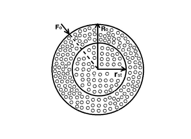
Example. Let us consider PEM in the form of a circle (ring) with a radius $R_{0}$ (see Fig. 1). We assume that all pores in the circle are connected by capillaries/fibers (this is not shown on the picture), saturated by water and the system is in steady-state (the gravity force is not taken into account). At the time moment $t=0$, a load $F_{0}$ begins to shrink (squeeze) the circle in the radially-symmetric direction. As a result, the boundary of the circle starts to move and simultaneously one expects a water outflow throughout the moving boundary. In the porous circle, the diffusion process of the water towards the boundary takes place. At the time moment $t=T$, the load stops to act. Finally, one obtains new porous circle with a radius $r_{st}<R_{0}$. In new steady-state, the porosity of the circle will be smaller because we assume a constant pressure $p_{a}$ at the ring surface all time, however, the matrix volume (actually it is the square) is still the same as at the moment $t=0$.

Refer to caption

Figure 1: Poroelastic material in the form of a circle (ring) with the initial radius $R_{0}$ and the radius $r_{st}$ after deformation caused by the load $F_{0}$.

Refer to caption

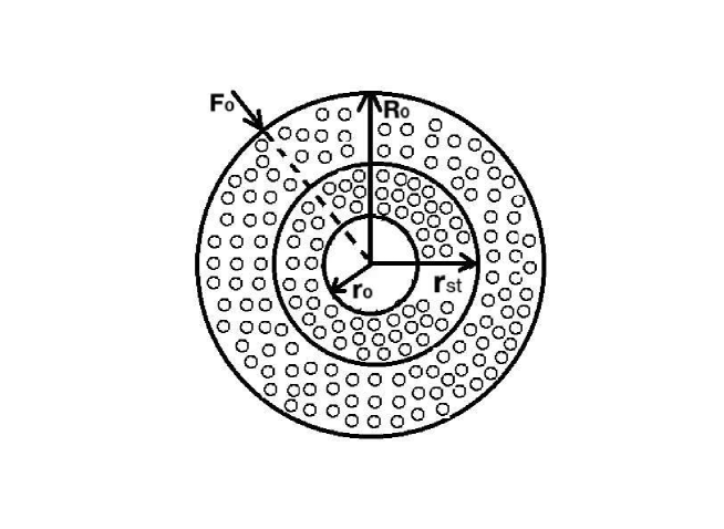
Figure 2: Poroelastic material in the form of an annulus with the initial outer radius $R_{0}$ and the radius $r_{st}$ after deformation caused by the load $F_{0}$.

The process described above allow us to simplify the governing Eqs. (42). In fact, deformation will take place only in the radially-symmetric direction, while the tangential deformation is zero (or negligibly small), therefore one may set $w^{2}=0$, i.e. the third equation in (45) vanishes. Moreover, we consider pure water, i.e. there is no solute transport, therefore the last equation can be skipped because one may set $C=0$. As a result, the mathematical model describing the deformation of PEM in the form of the circle consists of the following governing equations

$$\begin{array}[]{l}w_{tr}+\frac{1}{r}w_{t}=\frac{k}{2}\left(P_{rr}+\frac{1}{r}\,P_{r}\right),\vskip 6.0pt plus 2.0pt minus 2.0pt\\ w_{t}\Big{(}\varrho_{t}+\varrho w_{tr}+\frac{1}{r}\varrho w_{t}\Big{)}+\varrho w_{tt}=-P_{r}+\lambda^{*}w_{rr}+\frac{\lambda^{*}}{r}\,w_{r}-\frac{\lambda^{*}}{r^{2}}w,\vskip 6.0pt plus 2.0pt minus 2.0pt\\ \varrho_{t}+\varrho_{r}w_{t}=k(\rho^{0}_{F}-\varrho)\left(P_{rr}+\frac{1}{r}\,P_{r}\right)\vskip 6.0pt plus 2.0pt minus 2.0pt\\ \Theta_{t}+\Theta_{r}w_{t}=k\left(1-\Theta\right)\left(P_{rr}+\frac{1}{r}\,P_{r}\right),\end{array}$$ (46)

where the notation $w=w^{1}$ is used.

In order to complete the mathematical model, one needs to specify boundary conditions and initial profiles.

The boundary conditions:

$$\begin{array}[]{l}r=0:\quad\frac{\partial P}{\partial r}=0,\ \frac{\partial\varrho}{\partial r}=0,\ \frac{\partial\Theta}{\partial r}=0,\ w=0,\\ \vskip 6.0pt plus 2.0pt minus 2.0pt\\ r=S(t):\quad P=p_{a},\ w=S(t)-R_{0},\end{array}$$ (47)

where $S(t)$ is an unknown function that depends essentially on the load $F_{0}$ and has the specified values $S(0)=R_{0}$ and $S(T)=r_{st}.$

The initial conditions:

$$t=0:\quad P=p_{a},\ \varrho=\varrho_{0}(r),\ \Theta=\Theta_{0}(r),\ w=0,$$ (48)

and the condition for the final displacement of the surface is

$$t=T:\quad w=r_{st}-R_{0},$$ (49)

where $\varrho_{0}(r)$ and $\Theta_{0}(r)<1$ are given positive functions and $R_{0}$ and $r_{st}$ are known positive constants.

In order to take into account the load (force per a unit volume) $F_{0}$ (generally speaking, it can be a function of time) acting on the moving boundary, we need to specify the Terzaghi effective stress tensor in the radially-symmetric case. Taking into account the assumption about radial symmetry and the the strain tensor matrix presented in [1] (see Appendix A) in the cylindrical coordinates, the matrix $\varepsilon$ (see (30)) is equivalent to the vector

$$\Big{(}\frac{\partial w}{\partial r},\frac{w}{r},0\Big{)}^{T}.$$ (50)

So, using formulae (28), (29) and (31), the Terzaghi effective stress tensor can be derived in the form

$$\Big{(}-P+\lambda^{*}\frac{\partial w}{\partial r}+\frac{\lambda}{r}w,-P+\lambda\frac{\partial w}{\partial r}+\frac{\lambda^{*}}{r}w,0\Big{)}^{T}.$$ (51)

It means that the tensor matrix $\tilde{\tau}_{ter}$ is a diagonal matrix with the nonzero elements

$$\tau_{11}=-P+\lambda^{*}\frac{\partial w}{\partial r}+\frac{\lambda}{r}w,\quad\tau_{22}=-P+\lambda\frac{\partial w}{\partial r}+\frac{\lambda^{*}}{r}w.$$

Because the load $F_{0}$ pushes the boundary only along the radius $r$, one readily obtains the condition $\tilde{\tau}_{ter}\bar{n}=-F_{0}$, where $\bar{n}=(1,0)$ is the normal to the boundary. So, we arrive at the additional boundary condition

$$r=S(t):\quad\lambda^{*}\frac{\partial w}{\partial r}+\frac{\lambda}{r}w=p_{a}-F_{0}.$$ (52)

Thus, we obtain the BVP with moving boundary that consists of the governing Eqs. (46), the boundary conditions (47), (52) and the initial conditions (48)–(49).

The above example can be generalized by replacing the circle by the annulus

$$\Omega=\{(r,\phi):\ r_{0}<r<R_{0};0\leq\phi<2\pi\}.$$

In this case, we may assume the Dirichlet conditions on the interior boundary of the annulus:

$$r=r_{0}:\quad P=p_{a},\ \varrho=\varrho_{0},\ \Theta=\Theta_{0},\ w=0.$$ (53)

The last condition in (53) means that the interior of the annulus is fixed, i.e. zero displacement at $r=r_{0}$.

Remark 5

A simpler example for a water-saturated soil layer is studied in [5] (see Chapter 5). The bone deformation was studied in [17] using the bone layer in the form of circle, however the authors have not presented the mathematical model in detail.

5 Stationary exact solution

Exact solving of the nonlinear BVP that was formulated above is a highly nontrivial problem. Here we consider the stationary case that can be treated in a straightforward way. In the stationary case, i.e. all unknown functions do not depend on the time variable, the nonlinear system (46) reduces to two linear second-order ODEs with the general solution

$$P=P_{0}+C_{0}\ln r,\quad w=\frac{C_{0}}{2\lambda^{*}}r\ln r+C_{1}r+C_{-1}r^{-1},$$ (54)

while $\varrho(r)$ and $\Theta(r)$ are arbitrary smooth function ($P_{0}$ and $C$ with indices are arbitrary constants).

Let us consider the above example for PEM in the form of the annulus $\Omega$. The stationary solution satisfies the boundary conditions (53) if :

$$\begin{array}[]{l}p_{a}=P_{0}+C_{0}\ln r_{0}\ \Leftrightarrow\ C_{0}=\frac{p_{a}-P_{0}}{\ln r_{0}},\\ \frac{p_{a}-P_{0}}{2\lambda^{*}}\,r_{0}+C_{1}r_{0}+C_{-1}\,r_{0}^{-1}=0\ \Leftrightarrow\ C_{-1}=\left(\frac{P_{0}-p_{a}}{2\lambda^{*}}-C_{1}\right)r_{0}^{2}.\end{array}$$

Let us assume that we have a steady-state (stationary) position of the annulus with the boundary conditions

$$r=r_{st}\,:\ P=p_{st},\ w=r_{st}-R_{0}.$$ (55)

Thus, using the above boundary conditions, we specify $P_{0}$ and $C_{1}$ as follows:

$$P_{0}+\frac{p_{a}-P_{0}}{\ln r_{0}}\,\ln r_{st}=p_{st}\ \Leftrightarrow\ P_{0}=\frac{p_{st}\ln r_{0}-p_{a}\ln r_{st}}{\ln r_{0}-\ln r_{st}},\ r_{st}\not=r_{0}.$$

In the case $r_{st}=r_{0}$, the condition $p_{st}=p_{a}$ takes place. From the second condition in (55)

$$\frac{p_{a}-P_{0}}{2\lambda^{*}\ln r_{0}}\,r_{st}\ln r_{st}-\frac{(P_{0}-p_{a})r_{0}^{2}}{2\lambda^{*}r_{st}}+C_{1}r_{st}+\left(\frac{P_{0}-p_{a}}{2\lambda^{*}}-C_{1}\right)\frac{r_{0}^{2}}{r_{st}}=r_{st}-R_{0},$$

one defines

$$C_{1}=\left(\frac{P_{0}-p_{a}}{2\lambda^{*}\ln r_{0}}\,r_{st}\ln r_{st}-\frac{P_{0}-p_{a}}{2\lambda^{*}}\frac{r_{0}^{2}}{r_{st}}+r_{st}-R_{0}\right)\frac{r_{st}}{r_{st}^{2}-r_{0}^{2}},$$

where $r_{st}\neq r_{0}$.

If $r_{st}=r_{0}$ then $r_{st}=R_{0}$ and $C_{1}$ is an arbitrary constant, therefore we arrive an unrealistic situation $r_{st}=R_{0}=r_{0}$, i.e. the annulus degenerates into a circle.

Thus:

$$\begin{array}[]{l}P=P_{0}+(p_{a}-P_{0})\frac{\ln r}{\ln r_{0}},\vskip 6.0pt plus 2.0pt minus 2.0pt\\ w=\frac{p_{a}-P_{0}}{2\lambda^{*}}\,r\frac{\ln r}{\ln r_{0}}+C_{1}r+\left(\frac{P_{0}-p_{a}}{2\lambda^{*}}-C_{1}\right)\frac{r_{0}^{2}}{r},\end{array}$$ (56)

where

$$P_{0}=\frac{p_{st}\ln r_{0}-p_{a}\ln r_{st}}{\ln r_{0}-\ln r_{st}}=p_{a}+\frac{p_{st}-p_{a}}{1-\frac{\ln r_{st}}{\ln r_{0}}},$$ (57)
$$C_{1}=\left(\frac{p_{st}-p_{a}}{2\lambda^{*}(\ln r_{0}-\ln r_{st})}\,\Big{(}r_{st}\ln r_{st}-\frac{r_{0}^{2}\ln r_{0}}{r_{st}}\Big{)}+r_{st}-R_{0}\right)\frac{r_{st}}{r_{st}^{2}-r_{0}^{2}}.$$

Substituting (57) into (56), we arrive at

$$\begin{array}[]{l}P=\frac{p_{st}\ln r_{0}-p_{a}\ln r_{st}}{\ln r_{0}-\ln r_{st}}-\frac{p_{st}-p_{a}}{\ln r_{0}-\ln r_{st}}\ln r,\\ w=\frac{1}{2\lambda^{*}}\frac{p_{st}-p_{a}}{\ln r_{0}-\ln r_{st}}\left(\frac{r_{0}^{2}}{r}\ln r_{0}-r\ln r\right)+C_{1}\left(r-\frac{r_{0}^{2}}{r}\right),\end{array}$$ (58)

where $r_{st}\neq r_{0}.$

Finally, we need to determine the parameter $r_{st}$ that is an analogue of the unknown function $S(t)$ in the nonstationary case. This can be done using a modification of the boundary condition (52) in the form

$$r=r_{st}:\quad\lambda^{*}\frac{\partial w}{\partial r}+\frac{\lambda}{r}w=-\frac{F_{0}(r)}{2\pi r}.$$ (59)

Substituting the function $w$ from (58) into (59), one obtains a cumbersome transcendent equation for finding $r_{st}$ that is omitted here.

A simpler situation occurs, if one applies the boundary conditions involving the Neumann condition (zero flux) for the pressure $P$:

$$r=r_{0}:\ \frac{\partial P}{\partial r}=0,\ w=0.$$

The above conditions immediately produce

$$\frac{\partial P}{\partial r}\Bigg{|}_{r=r_{0}}=\frac{C_{0}}{r_{0}}=0\ \Rightarrow\ C_{0}=0,$$
$$w\big{|}_{r=r_{0}}=C_{1}r_{0}+C_{-1}r_{0}^{-1}=0\ \Rightarrow\ C_{-1}=-C_{1}r_{0}^{2}.$$

Moreover, the boundary conditions (55) lead to

$$P_{0}=p_{st},\ C_{1}\left(r_{st}-r_{0}^{2}r_{st}^{-1}\right)=r_{st}-R_{0},$$

therefore we arrive at the exact solution

$$P=p_{st},\ w=\frac{r_{st}\left(r_{st}-R_{0}\right)}{r_{st}^{2}-r_{0}^{2}}\left(r-\frac{r_{0}^{2}}{r}\right),\quad r_{st}\neq r_{0}.$$ (60)

In order determine the parameter $r_{st}$, we use Eq. (59). In the case of the above function $w$, condition (59) reduces to the algebraic equation

$$2(\lambda+\mu)\frac{r_{st}\left(r_{st}-R_{0}\right)}{r_{st}^{2}-r_{0}^{2}}+2\mu\frac{r_{0}^{2}\left(r_{st}-R_{0}\right)}{r_{st}(r_{st}^{2}-r_{0}^{2})}=-\frac{F_{0}(r_{st})}{2\pi r_{st}}.$$

In the simplest case, $F_{0}=const$, the above equations reduces to the cubic polynomial

$$(\lambda+\mu)r_{st}^{3}+\Big{(}\frac{F_{0}}{4\pi}-(\lambda+\mu)R_{0}\Big{)}r_{st}^{2}+\mu r_{0}^{2}r_{st}-\Big{(}\frac{F_{0}}{4\pi}+\mu R_{0}\Big{)}r_{0}^{2}=0.$$ (61)

So, depending on coefficients, the above equation have one, two or three real roots. Notably, $r_{st}=R_{0}$ if $F_{0}=0$, i.e. there is no deformation because nothing is acting on the annulus.

The simplest nontrivial case occurs when $F_{0}=4\pi(\lambda+\mu)R_{0}$. In this case, it can be easily proved that there exists a unique positive root $r_{st}=r_{*}$ belonging to the interval $(r_{0},R_{0})$. Thus, one may claim that the annulus was shrinking before steady-state has arrived.

If $F_{0}>4\pi(\lambda+\mu)R_{0}$ then $r_{*}\in(r_{0},R_{0})$ as well. Let us prove this. Left-hand-side of (61) is the third-order polynomial $P(r_{st})$ with critical points satisfying the quadratic equation

$$3(\lambda+\mu)r_{st}^{2}+2\kappa r_{st}+\mu r_{0}^{2}=0,$$

where $\kappa=\frac{F_{0}}{4\pi}-(\lambda+\mu)R_{0}>0$. Solving the above equation, one obtains

$${r_{st}}_{+,-}=\frac{1}{3(\lambda+\mu)}\Big{(}-\kappa\pm\sqrt{\kappa^{2}-3(\lambda+\mu)\mu r_{0}^{2}}\Big{)}.$$

Now one realizes that real parts of both critical points are negative. The point ${r_{st}}_{-}$ is the point of a local maximum and ${r_{st}}_{+}$ is the point of a local minimum provided $\kappa^{2}-3(\lambda+\mu)\mu r_{0}^{2}>0$. So, the polynomial is a strictly increasing function for all ${r_{st}}>{r_{st}}_{+}$. In the case of complex values of ${r_{st}}_{\pm}$, the polynomial $P(r_{st})$ is a strictly increasing function on any interval. In both cases, the polynomial must have a real root $r_{*}$. Moreover, $r_{*}>{r_{st}}_{+}$ if ${r_{st}}_{+}$ is a real number and $r_{*}$ is a unique real root if ${r_{st}}_{+}$ is complex.

Finally, we simply calculate $P(r_{0})=r_{0}^{2}((\lambda+\mu)(r_{0}-R_{0})-\mu R_{0})<0$ and $P(R_{0})=\frac{F_{0}}{4\pi}(R_{0}^{2}-r_{0}^{2})>0$, therefore $r_{*}\in(r_{0},R_{0})$. Thus, the annulus was shrinking before steady-state has arrived.

6 Conclusions

A mathematical model for the poroelastic materials (PEM) with the variable volume is developed in multidimensional case. Governing equations of the model are constructed using the continuity equations, which reflect the well-known physical laws. The deformation vector is specified using the Terzaghi effective stress tensor. As a result, the model is based on a system of $n+4$ partial differential equations for unknown functions $\bar{u}=(u_{1},\dots,u_{n})$ (deformation vector),  ${\theta_{F}}$ (porosity),  ${\rho}$ (density),   $c$ (concentration) and $p$ (hydrostatic pressure) is constructed.

The model is studied in the $2D$ space approximation by analytical methods. Using the classical Lie method, it is proved that the governing equations, which form a nonlinear six-component system, admit highly nontrivial Lie symmetries leading to an infinite-dimensional Lie algebra. It is shown that the infinite-dimensional Lie algebra admits an extension in the case of PEM formed by isotropic material. Interestingly that the additional Lie symmetry has the same form as for the classical Navier–Stokes equations (in the $2D$ approximation).

The radially-symmetric case is studied in details. It is shown how correct boundary conditions are constructed in the case of PEM in the form of a ring that is shrinking (expanding). As a result, the BVP with a moving boundary describing the ring deformation is constructed. The relevant BVP for the annulus deformation is presented as well. The nonlinear problems obtained are analytically solved in the stationary case, using the standard method for solving ODEs. In particular, the analytical formulae for unknown deformations and an unknown radius of the annulus are calculated.

7 Acknowledgements

R.Ch. is grateful to John R.King and Kostas Soldatos (both from the University of Nottingham) for useful comments. R.Ch. acknowledges that this research was funded by the British Academy (Leverhulme Researchers at Risk Research Support Grant LTRSF-100025). V.D. acknowledges that his research was supported by a grant from the Simons Foundation (1290607).

References

  • [1] L. A. Taber, Nonlinear Theory of Elasticity. Applications in Biomechanics, World Scientific, New Jersey, 2004.
  • [2] B. Loret, F. M. F. Simoes, Biomechanical Aspects of Soft Tissue, CRC Press, Boca Raton, 2017.
  • [3] E. Detournay, A. H-D. Cheng. Fundamentals of Poroelasticity, in: Analysis and Design Methods, ed. C. Fairhust, Pergamon Press, Oxford, 1993.
  • [4] O. Coussy, Mechanics of Porous Continua, Wiley & Sons Ltd., 1995.
  • [5] O. Coussy, Mechanics and Physics of Porous Solids, Wiley & Sons Ltd., 2010.
  • [6] U. Lacis, G. A. Zampogna, S. Bagheri, A computational continuum model of poroelastic beds, in: Proceedings of the Royal Society A – Mathematical Physical and Engineering Sciences 473 (2017) 20160932.
  • [7] J. I. Siddique, et al., A Review of mixture theory for deformable porous media and applications, Appl. Sci. 7(9) (2017) 917.
  • [8] V. Guerriero, S. Mazzoli, Theory of effective stress in soil and rock and implications for fracturing processes: A review, Geosciences 11(3) (2021) 119.
  • [9] S. Speziale, S. Sivaloganathan, Poroelastic theory of transcapillary flow: Effects of endothelial glycocalyx deterioration, Microvasc. Res. 78(3) (2009) 432–441.
  • [10] S. Speziale, G. Tenti, S. Sivaloganathan, A poroelastic model of transcapillary flow in normal tissue, Microvasc. Res. 75(2) (2008) 285–295.
  • [11] F. Travascio, R. Serpieri. S. Asfour, Articular cartilage biomechanics modeled via an intrinsically compressible biphasic model: implications and deviations from an incompressible biphasic approach, in: Summer Bioengineering Conference 55614 (2013) V01BT55A004.
  • [12] D. R. Sowinski, et al., Poroelasticity as a model of soft tissue structure: Hydraulic permeability reconstruction for magnetic resonance elastography in silico, Front. Phys. 8 (2020) 617582.
  • [13] R. Cherniha, J. Stachowska-Pietka, J. Waniewski, A mathematical model for transport in poroelastic materials with variable volume: derivation, lie symmetry analysis, and examples, Symmetry 12 (2020) 396. https://doi.org/10.3390/sym12030396
  • [14] R. Cherniha, V. Davydovych, J. Stachowska-Pietka, J. Waniewski, A mathematical Mmodel for transport in poroelastic materials with variable volume: derivation, Lie symmetry analysis and examples. Part 2, Symmetry 14 (2022) 109. https://doi.org/10.3390/sym14010109
  • [15] R. Cherniha, J. Stachowska-Pietka, J. Waniewski, A mathematical model for two solutes transport in a poroelastic material and its applications, Commun. Nonlinear Sci. Numer. Simulat. 132 (2024) 107905 https://doi.org/10.1016/j.cnsns.2024.107905
  • [16] R. Cherniha, V. Davydovych, A. Vorobyova, New Lie symmetries and exact solutions of a mathematical model describing solute transport in poroelastic materials, Math. Comp. Appl. 29(3) (2024) 43.
  • [17] D. A. Narmoneva, J. Y. Wang, L. A. Setton, A noncontacting method for material property determination for articular cartilage from osmotic loading, Biophys. J. 81 (2001) 3066–3076.
  • [18] P. Li, M. Schanz, Wave propagation in a 1-D partially saturated poroelastic column, Geophys. J. Int. 184(3) (2011) 1341–1353.
  • [19] K. Terzaghi, Relation between soil mechanics and foundation engineering, in: Proceedings of the International Conference on Soil Mechanics and Foundation Engineering, Boston, 1936, 13–18.
  • [20] Bluman GW, Cheviakov AF and Anco SC. Applications of symmetry methods to partial differential equations. New York: Springer; 2010.
  • [21] Arrigo DJ. Symmetry analysis of differential equations. Hoboken, NJ: John Wiley & Sons, Inc; 2015.
  • [22] Cherniha R, Serov M, Pliukhin O. Nonlinear reaction-diffusion-convection equations: Lie and conditional symmetry, exact solutions and their applications. Boca Raton: CRC Press; 2018.
  • [23] R. Cherniha, J. Stachowska-Pietka, J. Waniewski, A mathematical model for fluid-glucose-albumin transport in peritoneal dialysis, Int. J. Appl. Math. Comput. Sci. 24(4) (2014) 837–851.
  • [24] S.P. Lloyd, The infinitesimal group of the Navier–Stokes equations, Acta Mech. 38 (1981) 83–98.
  • [25] R. Cherniha, V. Davydovych, Lie symmetries, reduction and exact solutions of the $(1+2)$-dimensional nonlinear problem modeling the solid tumour growth, Commun. Nonlinear Sci. Numer. Simulat. 80 (2020) 104980. https://doi.org/10.1016/j.cnsns.2019.104980