Accurate simulations of reionization using the reduced speed of light approximation

Abstract

The reduced speed of light approximation has been employed to speed up radiative transfer simulations of reionization by a factor of $\gtrsim 5-10$. However, it has been shown to cause significant errors in the HI-ionizing background near reionization’s end in simulations of representative cosmological volumes. This can bias inferences on the galaxy ionizing emissivity required to match observables, such as the Ly$\alpha$ forest. In this work, we show that using a reduced speed of light is, to a good approximation, equivalent to re-scaling the global ionizing emissivity in a redshift-dependent way. We derive this re-scaling and show that it can be used to “correct” the emissivity in reduced speed of light simulations. This approach of re-scaling the emissivity after the simulation has been run is useful in contexts where the emissivity is a free parameter. We test our method by running full speed of light simulations using these re-scaled emissivities and comparing them with their reduced speed of light counterparts. We find that for reduced speeds of light $\tilde{c}\geq 0.2$, the 21 cm power spectrum at $0.1\leq k/[h{\rm Mpc}^{-1}]\leq 0.2$ and key Ly$\alpha$ forest observables agree to within $20\%$ throughout reionization, and often better than $10\%$. Position-dependent time-delay effects cause inaccuracies in reionization’s morphology on large scales that produce errors up to a factor of $2$ for $\tilde{c}\leq 0.1$. Our method enables a factor of $5$ speedup of radiative transfer simulations of reionization in situations where the emissivity can be treated as a free parameter.

1 Introduction

Radiative transfer (RT) simulations are a crucial tool for studying the Epoch of Reionization (EoR). During this period, the first generation of hydrogen ionizing sources drove ionization fronts (I-fronts) into the neutral intergalactic medium (IGM), which later overlapped and produced a fully ionized IGM by $z=5-6$ [1, 2, 3]. RT simulations can self-consistently track the growth and overlap of ionized regions during reionization, and model in detail the physical conditions in the intergalactic medium (IGM) during the process [4, 5, 6, 7]. They also allow the physics of galaxies to be directly linked to IGM conditions, enabling observables that probe reionization to constrain the physics of high-redshift galaxies.

Despite being the most physically accurate method available to study reionization, RT simulations are also the most computationally expensive. Formally, the RT equation is a $7$-dimensional problem - three spatial, two angular, one frequency, and one time. Moreover, representative cosmological volumes ($\gtrsim[100{\rm Mpc}]^{3}$) typically contain millions of ionizing sources, further increasing the cost of RT. Several methods, including moment-based RT [8, 9, 10] and adaptive ray tracing [11, 12] have been developed to speed up the angular component of the problem and eliminate the direct scaling of computation time with the number of sources. For many applications, only one to a few frequency bins are required to accurately model IGM conditions [e.g. 13, 6, 14]. Sub-grid treatments of the clumping of the IGM on $\sim$ kpc scales [e.g. 15, 16] can allow for simulations to be run at relatively coarse spatial resolution, which helps to counter the computational scaling with number of spatial dimensions.

An common trick used to speed up the time-dependence of the RT equation is the reduced speed of light approximation (RSLA). The time step required to resolve the transfer of radiation on an Eulerian grid is

$$t_{\rm rad}\leq\frac{\Delta x_{\rm cell}}{c}$$ (1.1)

where $\Delta x_{\rm cell}$ is the cell width and $c$ is the speed of light. Often, $t_{\rm rad}$ is much smaller than any other timescale (such as hydro-dynamical or chemical timescales), meaning that it could be much larger without affecting the treatment of these other processes. Indeed, if the RT is done in post-processing (as in many applications), the only relevant timescales are those associated with the RT equation itself. In addition to $t_{\rm rad}$, these are (1) the cell-crossing time of ionization fronts (I-fronts) and (2) the timescale over which the source population and underlying density field evolve. The typical speed of I-fronts ($v_{\rm IF}$) is $1-2$ orders of magnitude lower than $c$ [17], and the galaxy population evolves on timescales of $10s-100s$ of Myr, much longer than typical values of $t_{\rm rad}$ ($\lesssim 1$ Myr).

The RSLA introduces a smaller speed of light, $\tilde{c}<c$, chosen as small as possible so that $t_{\rm rad}$ remains the smallest timescale in the problem. Because the number of time-steps is inversely proportional to $t_{\rm rad}$, this gives a direct computational speedup by a factor of $c/\tilde{c}$. The RSLA has been used in a number of contexts to dramatically increase computational efficiency of reionization RT simulations at various spatial scales [18, 19].

However, several recent works [20, 21, 22, 23] have noted that the RSLA fails in certain important regimes of reionization modeling. Ref. [20] argued that the RSLA should be used only to model local fluctuations in the ionizing background during reionization, but never the mean ionizing background itself. Supporting this point, Ref. [22] found that using the RSLA leads to an under-estimate of the ionizing background close to and after the end of reionization by as much as a factor of $\tilde{c}/c$. Most recently, Ref. [23] found that reionization models calibrated to reproduce recent Ly$\alpha$ forest observations at $5<z<6$(from Ref. [24]) using the RSLA yielded biased results for the galaxy ionizing emissivity required to match these measurements. In this work, we seek to understand the reasons for these issues and find a way to account for them.

The findings of Ref. [23] hint at a possible pathway to a solution. They found that in simulations with different values of $\tilde{c}$, the global ionizing emissivity $\dot{N}_{\rm em}(z)$ could be calibrated to reproduce measurements of the Ly$\alpha$ forest transmission at $z\leq 6$ (their Fig. 10). This suggests that perhaps the RSLA is, at least approximately, equivalent to a redshift-dependent re-scaling of $\dot{N}_{\rm em}$. In this work, we will show that this is indeed the case, and we will provide a formula for this re-scaling that can be applied to $\dot{N}_{\rm em}$ for any simulation that uses the RSLA. In situations where $\dot{N}_{\rm em}$ is being set by hand (as in Ref. [23]), or is a function of some set of free parameters, this re-scaling can be applied to $\dot{N}_{\rm em}$ in “post-processing”. Then, the simulation can be treated as if it had used the full speed of light and the re-scaled $\dot{N}_{\rm em}$.

This work is organized as follows: in §2, we use a simple analytic model to understand why the RSLA fails in certain situations, and derive the aforementioned re-scaling of $\dot{N}_{\rm em}$. In §3, we briefly describe our numerical methods for running RT simulations of reionization. In §4-5 we use simulations to test how well our approach works, and we conclude in §6. Throughout, we assume the following cosmological parameters: $\Omega_{m}=0.305$, $\Omega_{\Lambda}=1-\Omega_{m}$, $\Omega_{b}=0.048$, $h=0.68$, $n_{s}=0.9667$ and $\sigma_{8}=0.82$, consistent with Ref. [25] results. All distances are quoted in co-moving units unless otherwise specified. Throughout, we will work in units in which the speed of light is unity ($c=1$).

2 The Method

2.1 When and why does the RSLA fail?

We will first build intuition for when and why the RSLA fails using a simple analytic argument. In the early stages of reionization, the universe contains a collection of ionized “bubbles” surrounding isolated clusters of ionizing sources, and is otherwise fully neutral. The mean photo-ionization rate, $\Gamma_{\rm HI}$, inside one of these bubbles is

$$\Gamma_{\rm HI}=N_{\gamma}c\sigma_{\rm HI}$$ (2.1)

where $N_{\gamma}$ is the mean number density of ionizing photons inside the bubble, $c$ is the speed of light, and $\sigma_{\rm HI}$ is the HI-ionizing cross-section averaged over the ionizing spectrum. At some time $t$ after reionization starts, $N_{\gamma}$ is given by

$$N_{\gamma}(t)=\int_{0}^{t}dt^{\prime}[\dot{N}_{\rm em}(t^{\prime})-\dot{N}_{\rm abs}(t^{\prime})]$$ (2.2)

where $\dot{N}_{\rm em}$ is the emission rate of photons inside the bubble by sources and $\dot{N}_{\rm abs}$ is the absorption rate. The latter can be written as two terms,

$$\dot{N}_{\rm abs}=\dot{N}_{\rm abs}^{\rm ion}+\dot{N}_{\rm abs}^{\rm rec}$$ (2.3)

where $\dot{N}_{\rm abs}^{\rm ion}$ is the absorption rate by neutral gas at the edges of the bubble, and $\dot{N}_{\rm abs}^{\rm rec}$ is due to recombinations within the bubble.

We will first consider the limit where the absorption rate is dominated by ionizations of neutral H atoms, such that $\dot{N}_{\rm abs}^{\rm ion}>>\dot{N}_{\rm abs}^{\rm rec}$. This limit is a good approximation early in reionization when the ionized bubbles are much smaller than their recombination-limited Stromgren volumes and most ionized regions have not yet overlapped. The absorption rate can then be written as

$$\dot{N}_{\rm abs}(t)=\dot{N}_{\rm abs}^{\rm ion}(t)\approx\dot{N}_{\rm em}(t-R/c)$$ (2.4)

where we have approximated the ionized region as a spherical bubble with radius $R$. The quantity $t-R/c$ is the so-called “retarded time” at the boundary of the ionized region (the ionization front or I-front) relative to the sources near the bubble’s center. That is, photons emitted at time $t-R/c$ will reach the bubble’s edge and be absorbed at time $t$.

We next assume that $R/c$ is sufficiently small that both $\dot{N}_{\rm em}$ and $R$ can be approximated as constant across this length of time. In this limit, Eq. 2.2 evaluates to

$$N_{\gamma}=\dot{N}_{\rm em}\times(t-[t-R/c])=\dot{N}_{\rm em}\frac{R}{c}$$ (2.5)

Putting this into Eq. 2.1, we get

$$\Gamma_{\rm HI}=\dot{N}_{\rm em}\frac{R}{c}c\sigma_{\rm HI}=\dot{N}_{\rm em}R\sigma_{\rm HI}$$ (2.6)

In this limit, $\Gamma_{\rm HI}$ is independent of the speed of light, and we can get the right $\Gamma_{\rm HI}$ inside the bubble using the RSLA. Indeed, replacing $R$ in Eq. 2.6 with the mean free path to ionizing photons, $\lambda$, reveals that we have reproduced the so-called “local source approximation” with its well-known relationship between $\Gamma_{\rm HI}$, $\lambda$, and $\dot{N}_{\rm em}$ [e.g. Ref. 26].

Next, we consider the opposite limit, in which $\dot{N}_{\rm abs}^{\rm ion}=0$. In this case, either the bubble has reached its limiting Stromgren volume (in which case $\dot{N}_{\rm abs}^{\rm rec}\approx\dot{N}_{\rm em}$), or the universe is entirely ionized. Either way, the right-hand side of Eq. 2.2 will be independent of the speed of light, since neither $\dot{N}_{\rm em}$ nor $\dot{N}_{\rm abs}^{\rm rec}$ depend on it. Thus, $N_{\gamma}$ is independent of $c$, and we have

$$\Gamma_{\rm HI}\propto c$$ (2.7)

Thus, using the RSLA in this limit would result in $\Gamma_{\rm HI}$ being incorrect by the same factor by which $c$ is reduced.

The first approximation - that $\dot{N}_{\rm abs}^{\rm ion}$ dominates the absorption rate - is valid near the beginning of reionization, as we mentioned earlier. The reason $\Gamma_{\rm HI}$ is independent of $c$ in this limit is that the time required for photons to reach neutral gas is proportional to $1/c$, such that $N_{\gamma}$ inside the bubble(s) is also proportional to this factor. This cancels the factor of $c$ in Eq. 2.1, which gives the correct $\Gamma_{\rm HI}$ if a reduced $c$ is used, even though $N_{\gamma}$ is incorrect. In the other limit, the fact that $N_{\gamma}$ is independent of $c$ means that it will still be correct when a reduced $c$ is used, causing $\Gamma_{\rm HI}$ to be incorrect. The first limit is expected to apply near the beginning of reionization, and the second near and after its end. The limiting behavior described here is exactly what was found in Ref. [22] (see also Ref. [21]).

2.2 Fixing the problem

In this section, we will show that, to a good approximation, the use of the RSLA equivalent to a redshift-dependent re-scaling of $\dot{N}_{\rm em}$. Consider two simulations, one using the full speed of light $\tilde{c}=c=1$ and the other a reduced speed of light $\tilde{c}<1$. Let these simulations have global ionizing emissivities $\dot{N}_{\rm em}^{c}$ and $\dot{N}_{\rm em}^{\tilde{c}}$, respectively. Our goal is to find a relationship between these four quantities such that these two simulations have identical physical properties - including reionization history, net absorption rate, $\Gamma_{\rm HI}$, etc. In particular, if they have the same absorption rate (that is, $\dot{N}_{\rm abs}^{c}=\dot{N}_{\rm abs}^{\tilde{c}}$), then from Eq. 2.2, we have

$$N_{\gamma}^{c}(t)-\int_{0}^{t}dt^{\prime}\dot{N}_{\rm em}^{c}(t^{\prime})=N_{\gamma}^{\tilde{c}}(t)-\int_{0}^{t}dt^{\prime}\dot{N}_{\rm em}^{\tilde{c}}(t^{\prime})$$ (2.8)

where we have used the same speed-of-light notation for $N_{\gamma}$ that we did for $\dot{N}_{\rm em}$. If we also assume that both simulations have the same mean $\Gamma_{\rm HI}$, then from Eq. 2.1 we have

$$N_{\gamma}^{c}c\sigma_{\rm HI}=N_{\gamma}^{\tilde{c}}\tilde{c}\sigma_{\rm HI}\rightarrow N_{\gamma}^{c}=N_{\gamma}^{\tilde{c}}\frac{\tilde{c}}{c}$$ (2.9)

Provided Eq. 2.9 holds at all times, we can differentiate both sides with respect to time to get

$$\dot{N}_{\gamma}^{c}=\dot{N}_{\gamma}^{\tilde{c}}\frac{\tilde{c}}{c}$$ (2.10)

Differentiating both sides of Eq. 2.8 with respect to time and substituting for $N_{\gamma}^{c}$ using Eq. 2.10 yields the main result of this paper,

$$\boxed{\dot{N}_{\rm em}^{c}(t)=\dot{N}_{\rm em}^{\tilde{c}}(t)-\dot{N}_{\gamma}^{\tilde{c}}(t)\left(1-\frac{\tilde{c}}{c}\right)}$$ (2.11)

We have explicitly written the time dependence to emphasize that Eq. 2.11 holds at all times.

Eq. 2.11 expresses the emissivity in the simulation with the full speed of light in terms of $c$, $\tilde{c}$, $N_{\rm em}^{\tilde{c}}$, and $\dot{N}_{\gamma}^{\tilde{c}}$. The first two of these are just numbers, and the other two are known after the simulation with the reduced speed of light has been run. This allows us to calculate $\dot{N}_{\rm em}^{c}$ without running any simulations with the full speed of light. Again, $\dot{N}_{\rm em}^{c}$ is the emissivity would produce (approximately) the same ionization history, $\Gamma_{\rm HI}$, etc. as the reduced speed of light run, had the full speed of light been used. Of course, since we had to assume that this relationship exists in order to derive Eq. 2.11, we have not yet proven that this statement is true. We will do so using RT simulations in §4-5.

The usefulness of Eq. 2.11 is found in situations where $\dot{N}_{\rm em}$ is being treated as a “free parameter”, which can be “corrected” after the simulation has been run. Indeed, in works such as Refs. [3, 6, 16], $\dot{N}_{\rm em}$ is a “free function” of redshift that is set by hand to match some set of observables - in those works, the mean transmission of Ly$\alpha$ forest at $z\leq 6$. In many semi-numerical frameworks [e.g. 21cmFAST, Refs. 29, 30], $\dot{N}_{\rm em}$ is uniquely determined by a set of free parameters that are being constrained using a set of observations. In this case, a re-scaling of $\dot{N}_{\rm em}$ corresponds to changing the mapping between these parameters and $\dot{N}_{\rm em}$ in a way that can be quantified. We emphasize the Eq. 2.11 does not constitute a correction to the RSLA simulation results themselves, but rather simply a re-scaling of the global emissivity after the simulation has been run. As such, it is unfortunately not directly applicable in situations where $\dot{N}_{\rm em}$ is a self-consistent prediction of e.g. an underlying galaxy model [5, 19, 7]. In this situation, one would require a method to correct the simulation quantities themselves, which is beyond the scope of this work.

3 Numerical Methods

Our simulations are run with the adaptive ray-tracing RT code FlexRT, first described in [16, 31] and tested in Ref. [32]. Here, we will briefly discuss the relevant features of the code, referring the reader to these works for details. FlexRT solves the RT equation in post-processing on a time-series of cosmological density fields. We model the ionizing sources in a simple manner by extracting halos from an N-body simulation with the same large-scale structure as the density field and assigning them ionizing emissivities (see below). The RT equation itself is solved using an adaptive ray tracing method similar to the one described in Ref. [11] and employed in the code of Ref. [12]. Sub-resolved ionization fronts are tracked using the “moving-screen” approximation, and the temperature behind them ($T_{\rm reion}$) is estimated using the flux-based method described in Ref. [17]. FlexRT solves for the opacity of the ionized IGM to ionizing photons using a novel sub-grid model based on high-resolution hydro/RT simulations of IGM gas dynamics similar to those described in Refs. [18, 27]. Recent improvements to this model, and details about forward-modeled observables are detailed in Ref. [23].

In §4, we will use the “Reference” setup in Ref. [23], which assumes a fully dynamically relaxed IGM and mono-chromatic RT. The physical properties of this model are summarized in their Fig. 2 and associated text. Throughout in §4, the only parameters we will change relative to their Reference model are $\dot{N}_{\rm em}$ and $\tilde{c}$. We will generalize and test Eq. 2.11 in the context of multi-frequency RT simulations in §5. Our simulations have a box size of $L=200$ $h^{-1}$Mpc with $N_{\rm RT}=200^{3}$ RT cells. Ly$\alpha$ forest properties are calculated (following §3.7 of Ref. [23]) on a high-resolution ($N=2048^{3}$) hydrodynamics simulation with the same large-scale initial conditions used for the N-body simulation from which we get the halos. In this work, we will consider reduced speeds of light of $\tilde{c}=0.05$, $0.1$, $0.2$, $0.3$, and $0.5$, alongside simulations that use the full speed of light ($\tilde{c}=c=1$).

4 Testing the Method

4.1 Strategy & Terminology

The claim of Eq. 2.11 can be summarized as follows: Given an RT simulation run with a reduced speed of light $\tilde{c}$ and emissivity $\dot{N}_{\rm em}^{\tilde{c}}(z)$ that has a mean photon number density $N_{\gamma}^{\tilde{c}}(z)$, a simulation using the full speed of light and emissivity $\dot{N}_{\rm em}^{c}(z)$ should have the same reionization history, ionization morphology, IGM transmission properties, etc. as the original simulation. We can verify whether this claim is true by comparing two types of simulations. We first run simulations using the RSLA, with $\tilde{c}<1$. We refer to these simply as reduced-$c$ runs, with emissivity $\dot{N}_{\rm em}^{\tilde{c}}$. Next, we apply the re-scaling in Eq. 2.11 to $\dot{N}_{\rm em}^{\tilde{c}}$ to obtain $\dot{N}_{\rm em}^{c}$, and run another simulation with the full speed of light using $\dot{N}_{\rm em}^{c}$. We refer to these as full-$c$, re-scaled $\dot{N}_{\rm em}$ runs. Eq. 2.11 is accurate to the extent that the properties of these two types of simulations agree with each other. Lastly, for purposes of comparison, we will also include a third type of simulation, in which we use the full speed of light but do not apply any re-scaling to $\dot{N}_{\rm em}^{\tilde{c}}$. We refer to these as full-$c$, un-scaled $\dot{N}_{\rm em}$ runs. We summarize the properties of these three types of simulations in Table 1.

Name	Emissivity	Speed of Light	Description
			Simulation using reduced
Reduced-$c$	$\dot{N}_{\rm em}^{\tilde{c}}$	$\tilde{c}<1$	speed of light using
			un-scaled emissivity
			Full speed of light
full-$c$, re-scaled $\dot{N}_{\rm em}$	$\dot{N}_{\rm em}^{c}$ (Eq. 2.11)	$\tilde{c}=c=1$	simulation with $\dot{N}_{\rm em}$
			re-scaled using Eq. 2.11
			Full speed of light
			simulation, but using
full-$c$, un-scaled $\dot{N}_{\rm em}$	$\dot{N}_{\rm em}^{\tilde{c}}$	$\tilde{c}=c=1$	$\dot{N}_{\rm em}$ from the
			Reduced-$c$ run without
			any re-scaling applied

Table 1: Summary of different kinds of simulations referred to in this work, and the names used for each (left-most column). The second column from left gives the emissivity used in that simulation, and the third column the speed of light. The right-most column briefly describes each type of simulation.

4.2 Ionization history and morphology

We begin by studying how well the reionization history and morphology (shapes and sizes) of ionized regions match in the reduced-$c$ and full-$c$, re-scaled $\dot{N}_{\rm em}$ runs. For this section, we scale up $\dot{N}_{\rm em}$ from the reference model of Ref. [23] until reionization ends at $z\approx 6$ when $c=1$. This is our full-$c$, un-scaled $\dot{N}_{\rm em}$ run. Next, we use the same $\dot{N}_{\rm em}$ to run a series of reduced-$c$ runs with $\tilde{c}=0.05$, $0.1$, $0.2$, $0.3$, and $0.5$. Lastly, we evaluate Eq. 2.11 for each of these and then run a set of full-$c$, re-scaled $\dot{N}_{\rm em}$ simulations. Again, the degree to which the reduced-$c$ and corresponding full-$c$, re-scaled $\dot{N}_{\rm em}$ runs agree with each other determines how accurate is Eq. 2.11.

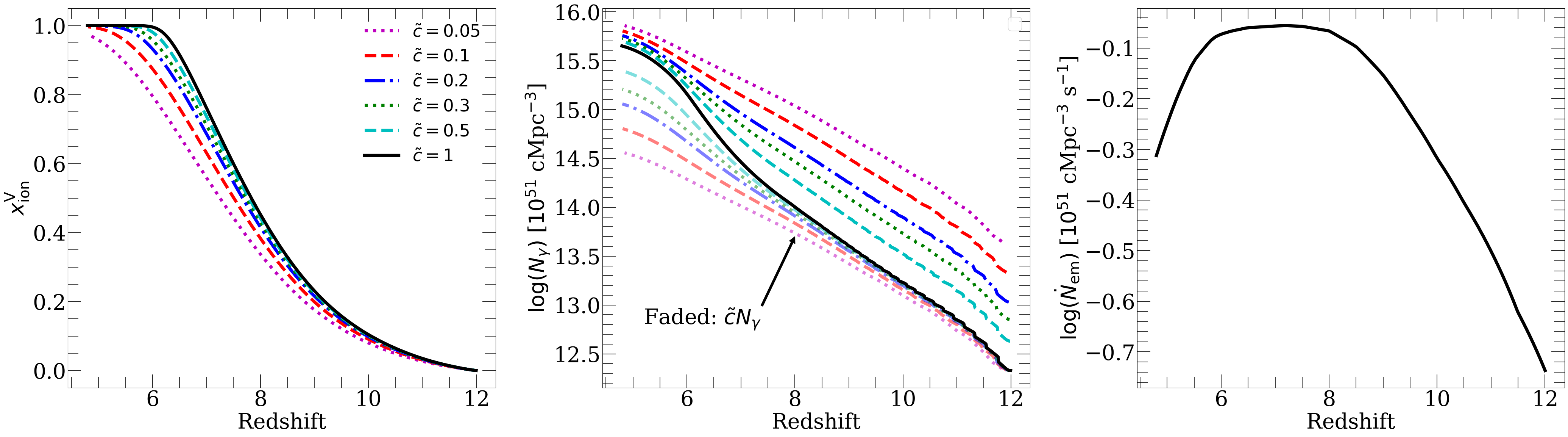
Figure 1: Summary of full-$c$, un-scaled $\dot{N}_{\rm em}$ and reduced-$c$ simulations used to study how well Eq. 2.11 works with respect to the reionization history and morphology. Left: the reionization history for each value of $\tilde{c}$, using a scaled-up version of $\dot{N}_{\rm em}$ from the reference model from Ref. [23], which ends reionization at $z=6$ for $\tilde{c}=c=1$ (black solid curve, the full-$c$, un-scaled $\dot{N}_{\rm em}$ run). Reducing $\tilde{c}$ pushes the end of reionization later, such that it has not finished by $z=4.8$ for $\tilde{c}=0.05$. Middle: number density of ionizing photons, $N_{\gamma}$. The thick lines denote the actual values, while the faded lines show $\tilde{c}N_{\gamma}$. Consistent with our analytic argument in §2.1, at the beginning of reionization $\dot{N}_{\gamma}$ is a factor of $1/\tilde{c}$ higher in the reduced-$c$ runs than in the full-$c$, un-scaled $\dot{N}_{\rm em}$ case (Eq. 2.5). Near reionization’s end, they approach similar values. Right: Ionizing emissivity used in all these simulations ($\dot{N}_{\rm em}^{\tilde{c}}$).

4.2.1 Ionization history

In Figure 1, we show the volume-averaged ionized fraction $x_{\rm ion}^{\rm V}$ (left), the ionizing photon number density $\dot{N}_{\gamma}$ (middle), and the ionizing emissivity $\dot{N}_{\rm em}$ (right) for our full-$c$, un-scaled $\dot{N}_{\rm em}$ run (black solid curve) and our reduced-$c$ runs (colored curves, see legend). In the left panel, we see that the reionization histories are initially similar, but start to diverge as reionization enters its later stages. The end of reionization is delayed by $\Delta z\approx 1.5$ in the $\tilde{c}=0.05$ simulation relative to the $\tilde{c}=1$ case. The bold curves in the middle panel show $\dot{N}_{\gamma}$ for each simulation, while the faded curves show $\tilde{c}N_{\gamma}$. Early in reionization, $\dot{N}_{\gamma}$ scales linearly with $1/\tilde{c}$, consistent with the early reionization limit described by Eq. 2.5. However, as reionization ends, $\dot{N}_{\gamma}$ for all simulations approaches the same value, reflecting the behavior expected near reionization’s end in §2.1. The right-most panel shows $\dot{N}_{\rm em}^{\tilde{c}}$, which is the same for all the simulations shown here.

In the left panels Figure 2, we compare each of our reduced-$c$ runs to their full-$c$, re-scaled $\dot{N}_{\rm em}$ counterparts. We show the former as bold curves and the latter as faded curves, with the color and line style identifying the value of $\tilde{c}$. The upper left panel shows $x_{\rm ion}^{\rm V}$, zoomed in on the second half of the reionization history for clarity. We find excellent agreement between the two even for our lowest value of $\tilde{c}=0.05$, such that the different sets of curves are difficult to see on the plot. The bottom left panel shows the linear differences of $x_{\rm ion}^{\rm V}$ in the reduced-$c$ and full-$c$, re-scaled $\dot{N}_{\rm em}$ runs over the entire reionization history. For all but the $\tilde{c}=0.05$ case, the difference is always $\lesssim 0.01$, and for $\tilde{c}\geq 0.3$ it is $<0.005$.

In the upper right panel, we show $\dot{N}_{\rm em}^{c}$ calculated using Eq. 2.11, and the bottom right panel shows the ratio with $\dot{N}_{\rm em}^{\tilde{c}}$ (the black solid curve). This ratio differs from unity the most at the end of reionization, dropping to $\approx 0.5$ ($0.8$) by $z=5$ for $\tilde{c}=0.05$ ($0.5$). The fact that the reduced-$c$ and full-$c$, re-scaled $\dot{N}_{\rm em}$ runs have such different $\dot{N}_{\rm em}$ but similar reionization histories validates Eq. 2.11. As we will see, the small differences in reionization history arise because Eq. 2.11 applies to globally averaged quantities, and does not account for spatial fluctuations in the distribution of photons in the IGM.

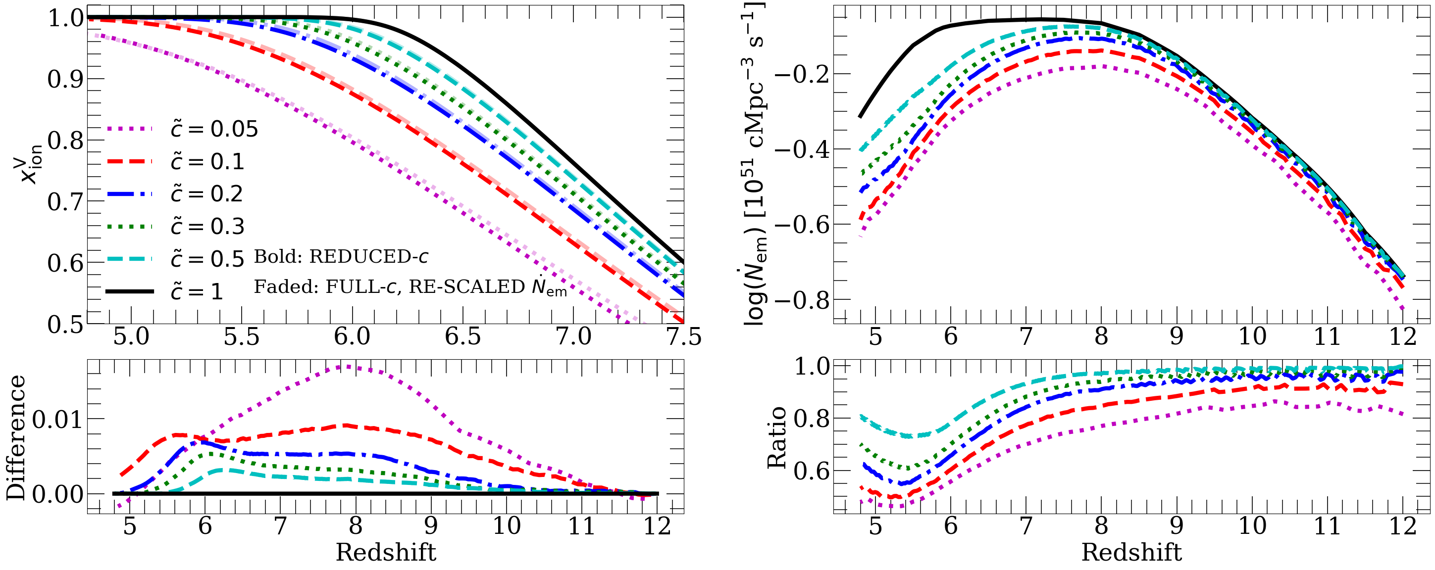
Figure 2: Comparison of the reionization history and emissivity in our reduced-$c$ and full-$c$, re-scaled $\dot{N}_{\rm em}$ simulations. Upper Left: the same reionization histories (again), but zoomed in on the last half of reionization and including the full-$c$, re-scaled $\dot{N}_{\rm em}$ results for each value of $\tilde{c}$ (faded curves). The bold and faded curves agree very well for all values of $\tilde{c}$, such that they are difficult to tell apart on the plot. Lower Left: the linear differences between $x_{\rm ion}^{\rm V}$ for the reduced-$c$ and corresponding full-$c$, re-scaled $\dot{N}_{\rm em}$ runs. This is less than $0.01$ for all except $\tilde{c}=0.05$. Upper Right: emissivities for each of the full-$c$, re-scaled $\dot{N}_{\rm em}$ runs ($\dot{N}_{\rm em}^{c}$ from Eq. 2.11, colored curves) compared to $\dot{N}_{\rm em}^{\tilde{c}}$ (black solid curve). Bottom Right: ratio of $\dot{N}_{\rm em}^{c}$ and $\dot{N}_{\rm em}^{\tilde{c}}$ for each $\tilde{c}$. The ratio is smallest at the end of reionization, dropping to $0.5$ ($0.8$) for $\tilde{c}=0.05$ ($0.5$).

These results show that, at least with respect to the global ionization history, the claim of Eq. 2.11 is reasonably accurate. Namely, that using the RSLA is equivalent to a redshift-dependent re-scaling of $\dot{N}_{\rm em}$. We emphasize again that Eq. 2.11 does not prescribe a way to directly correct the reduced-$c$ simulation results for the effects of the RSLA. Put another way, we do not prescribe a way to convert the reduced-$c$ results into those of the full-$c$, un-scaled $\dot{N}_{\rm em}$ results. As such, our method is not directly applicable when $\dot{N}_{\rm em}$ is a prediction of e.g. some underlying galaxy model.

4.2.2 Ionization morphology

Next, we apply the same analysis to the morphology of ionized and neutral regions, and statistics that depend on it. Figure 3 shows maps of the ionization field when the universe is $80\%$ ionized for reduced-$c$ (top row) and full-$c$, un-scaled $\dot{N}_{\rm em}$ runs (middle row). Dark regions are neutral and white ones are ionized. The bottom row shows the difference maps for the top and middle rows. Red (blue) denotes regions that are more neutral (ionized) in the reduced-$c$ simulations.

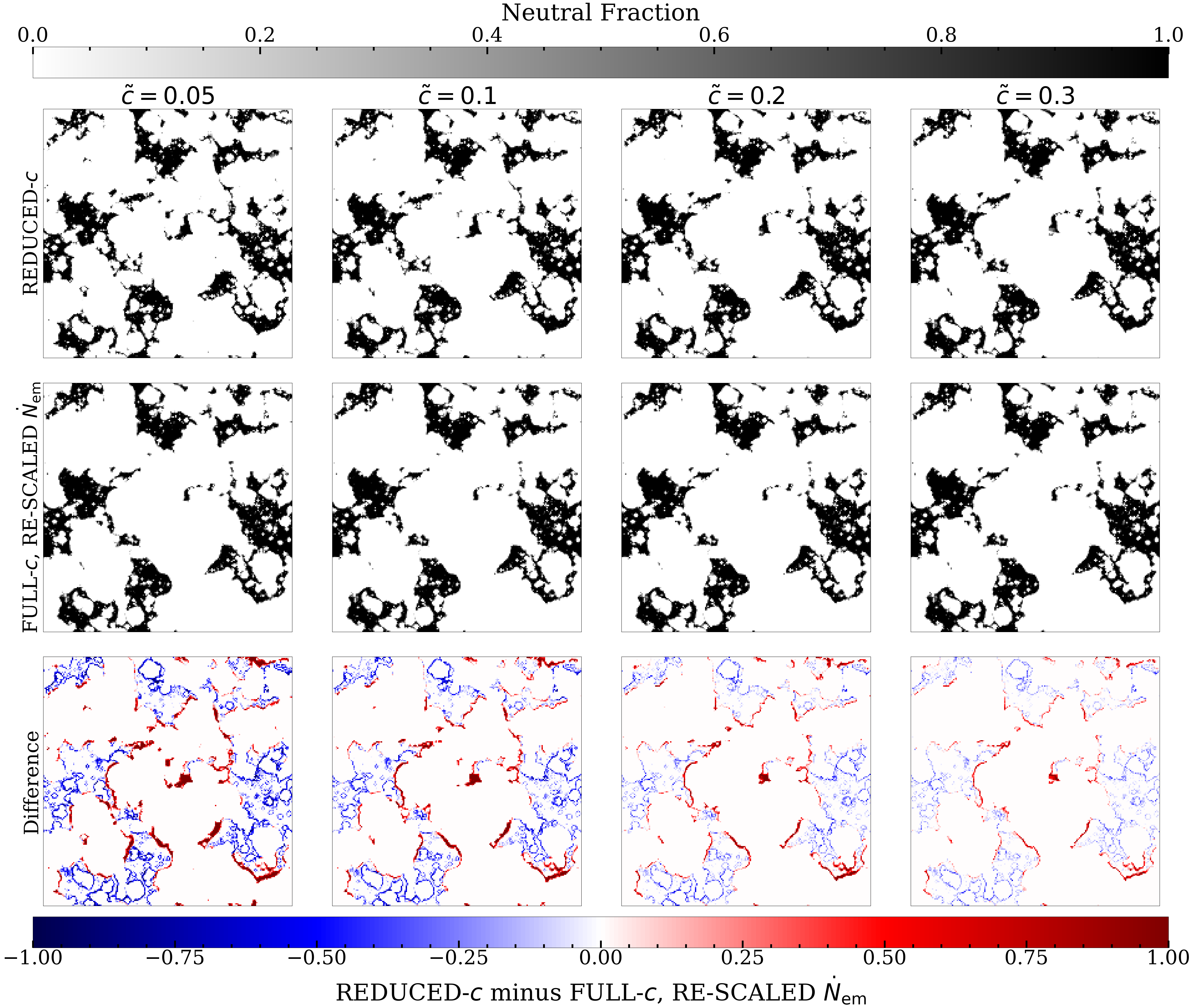
Figure 3: Visualization of the ionization field at $80\%$ ionized in reduced-$c$ (top row) and full-$c$, re-scaled $\dot{N}_{\rm em}$ runs (middle row) for $\tilde{c}=0.05$, $0.1$, $0.2$, and $0.3$ (left to right). We show the difference maps for each value of $\tilde{c}$ in the bottom row. We see in the top row that as $\tilde{c}$ decreases (right to left), the neutral regions (islands) become more extended and porous at fixed ionized fraction. We do not see this in the middle row, indicating that it is not due to differences in the reionization history between reduced-$c$ runs. Instead, it is because the RSLA induces a longer delay between emission and absorption for photons emitted in large vs. small ionized bubbles. The re-scaling in Eq. 2.11 corrects for the delay only on average, and does not account for position dependence. The result is that the morphologies in the reduced-$c$ and full-$c$, re-scaled $\dot{N}_{\rm em}$ runs diverge as $\tilde{c}$ decreases.

From right to left (decreasing $\tilde{c}$) in the top row, the neutral regions (islands) grow slightly more extended and porous. Equivalently, the smallest ionized bubbles grow larger, and the largest ones smaller, when $\tilde{c}$ decreases. We see no such trend, however, in the middle row. From this, we deduce that the morphological differences in the top row are not due to the reduced-$c$ runs having different reionization histories, since such differences would appear for the full-$c$, re-scaled $\dot{N}_{\rm em}$ also. They are instead a position-dependent artifact of the RSLA. Photons emitted in large ionized regions experience a longer delay between emission and absorption than do those emitted in small bubbles. Eq. 2.11 accounts for this time-delay only on average, and thus misses the differences between photons emitted in different regions. As a result, the largest (smallest) bubbles are too small (large) in the reduced-$c$ runs. We can most clearly see this effect in the difference maps, where it is clearly visible even for $\tilde{c}=0.3$. In this work, we do not attempt to correct for this position-dependent effect, since doing so would be complicated by the non-locality of the ionizing radiation field. As we will see, this effect will set the minimum value of $\tilde{c}$ for which Eq. 2.11 can be used.

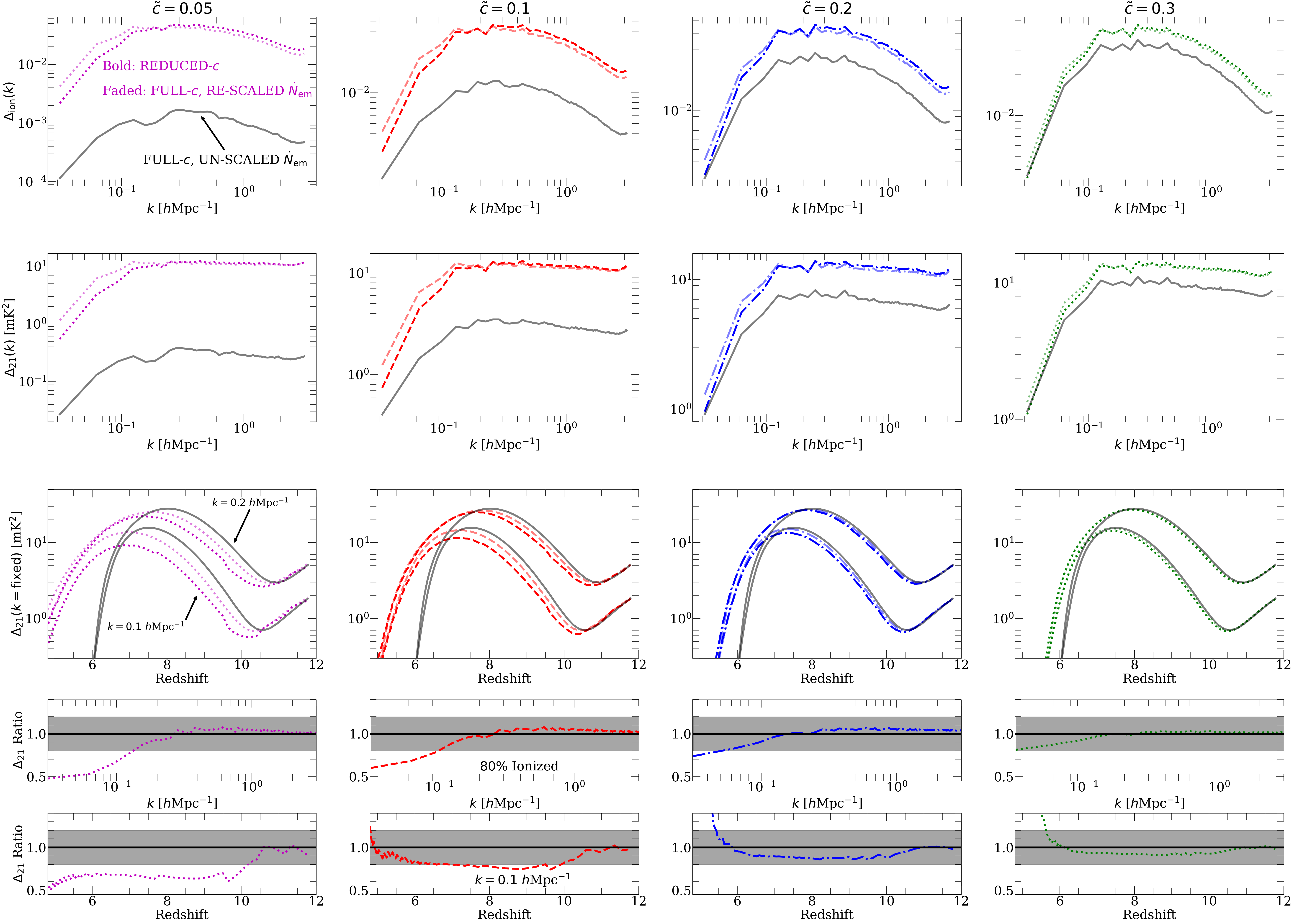
Figure 4: Power spectrum of the ionization field and 21 cm signal for simulations with $\tilde{c}=0.05$, $0.1$, $0.2$, and $0.3$ (columns from left to right). Top Row: power spectrum of the ionization field, $\Delta_{\rm ion}$, vs. wavenumber $k$ at an ionized fraction of $80\%$. The bold colored curves show results for the reduced-$c$ simulations, and the faded colored curves the full-$c$ re-scaled runs. The faded gray curves shows (at fixed redshift) the full-$c$, un-scaled $\dot{N}_{\rm em}$ runs. 2nd Row: the same, but for the 21 cm power spectrum, $\Delta_{21}$. The full-$c$, un-scaled $\dot{N}_{\rm em}$ results differ dramatically from the other two, reflecting its lower neutral fraction at fixed redshift. However, the reduced-$c$ and full-$c$, re-scaled $\dot{N}_{\rm em}$ runs differ in their shape: the former has significantly less power on large scales (small $k$) and slightly more on small-scales (large $k$). 3rd Row: $\Delta_{21}$ vs redshift at $k=0.2$ and $0.1$ $h$Mpc^-1 (top and bottom set of curves, respectively). The bold colored curves are noticeably below the faded ones, reflecting the deficit in large-scale power in the reduced-$c$ runs. 4th & 5th Rows: ratios of the reduced-$c$ and full-$c$ re-scaled results in the 2nd and 3rd rows, respectively. The shaded regions denote $\pm 20\%$ from unity. In the bottom row, we show the ratio for $k=0.1$ $h$Mpc^-1. Decreasing $\tilde{c}$ increases differences at low $k$, so that for $\tilde{c}=0.1$ the difference is $\approx 20\%$ at all redshifts at $k=0.1$ $h$Mpc^-1. At $\tilde{c}\geq 0.2$, we find $\lesssim 15\%$ differences at $k=0.1$ $h$Mpc^-1, which get smaller at larger $k$.

Figure 4 quantitatively compares the large-scale fluctuations in the ionization field in all three types of simulations. In the top row, we show the dimensionless ionization power spectrum $\Delta_{\rm ion}(k)$ at $80\%$ ionized for $\tilde{c}=0.05$, $0.1$, $0.2$, and $0.3$ (left to right). The bold colored lines, faded colored lines, and faded gray lines indicate results for reduced-$c$, full-$c$, re-scaled $\dot{N}_{\rm em}$, and full-$c$, un-scaled $\dot{N}_{\rm em}$ runs, respectively. The second row is the same thing, but instead showing the 21 cm power spectrum, calculated using the tools21cm package of Ref. [33].

The power in the full-$c$, un-scaled $\dot{N}_{\rm em}$ run is much lower than the others - increasingly so at lower $\tilde{c}$. This reflects the fact that the reduced-$c$ runs are more delayed relative to the full-$c$, un-scaled $\dot{N}_{\rm em}$ case the smaller $\tilde{c}$ is. So, at a fixed neutral fraction in the former, the neutral fraction in the latter decreases for smaller $\tilde{c}$. The full-$c$, re-scaled $\dot{N}_{\rm em}$ sims are much closer to the reduced-$c$ results, but differ noticeably in their shape. The latter have significantly less power at large scales (small $k$), and slightly more power at small scales (large $k$). This is a direct result of the morphological errors shown in Figure 3, with the reduced sizes of the largest bubbles driving the decrease in small-$k$ power. In the third row, we show $\Delta_{21}$ vs. redshift at fixed $k=0.2$ and $0.1$ $h$Mpc^-1 (top and bottom set of curves, respectively), key targets for experiments such as HERA [34, 35, 36]. The suppression in power is consistent across the entire reionization history, indicating that even early in reionization the RSLA can cause significant errors in ionization morphology.

The fourth row shows the ratio of the bold and faded colored curves in the second row, with the shaded region denoting $\pm 20\%$. For $\tilde{c}=0.3$, the differences between the reduced-$c$ and full-$c$ re-scaled runs never exceeds $20\%$ even at the largest scales at $80\%$ ionized. For lower $\tilde{c}$, the drop in power at small $k$ increases, reaching a factor of $\approx 2$ at the box scale for $\tilde{c}=0.05$. For $\tilde{c}=0.2$ the deviation is still only $\sim 10\%$ at $k=0.1$ $h$Mpc^-1, but at $\tilde{c}=0.1$ this increases to $20\%$, and to $30\%$ for $\tilde{c}=0.05$. The bottom row shows the ratio of the $k=0.1$ $h$Mpc^-1 curves in the third row. Here we see that for $\tilde{c}=0.2$, the differences are never larger than $15\%$ at any redshift. For $\tilde{c}=0.1$, the difference exceeds $20\%$ at $z\sim 9$, and for $\tilde{c}=0.05$, it reaches nearly a factor of $2$.

We see that the utility of Eq. 2.11 is limited by the fact that it does not account for the spatial fluctuations in the delay between emission and ionization of ionizing photons in the reduced-$c$ simulations. To summarize, $\Delta_{21}$ at $k\leq 0.1$ $h$Mpc^-1 can deviate by $20\%$ between the reduced-$c$ and full-$c$, re-scaled $\dot{N}_{\rm em}$ runs for $\tilde{c}=0.1$, and by up to $40\%$ for $\tilde{c}=0.05$. These differences drop to $\leq 15\%$ for $\tilde{c}=0.2$ and $\leq 10\%$ for $\tilde{c}=0.3$. As such, we caution against applying our method for $\tilde{c}<0.2$ in contexts where the large-scale reionization morphology is important.

4.3 QSO observations at $z\leq 6$

In this section, we apply the same kind of test to observables derived from high-redshift quasar absorption spectra at $z\leq 6$. These include the Ly$\alpha$ forest, which has recently yielded detailed insights into the tail end of reionization at $5<z<6$ [3, 6, 37, 30, 24], and the ionizing photon mean free path [38, 39, 40, 41]. These observables are sensitive not only to ionization morphology, but also to the large-scale spatial fluctuations in the ionizing background $\Gamma_{\rm HI}$ and the IGM temperature, which are affected by the RSLA.

4.3.1 Global Observables

The evolution of the mean transmission of the Ly$\alpha$ forest is a tight boundary condition on the end of reionization. Several studies [3, 42, 23, 14] have “calibrated” their reionization simulations to agree by construction with this observable, then asked whether other observables predicted by the simulation agree well with observations. Here, we will follow this procedure and assess how applicable Eq. 2.11 is in the context of forest-anchored studies. We first run a set of reduced-$c$ simulations with $\dot{N}_{\rm em}^{\tilde{c}}(z)$ calibrated so that the mean transmission of the Ly$\alpha$ forest matches the recent observations of Ref. [24]. Note that unlike in the previous section, this procedure yields a different $\dot{N}_{\rm em}^{\tilde{c}}$ for each value of $\tilde{c}$, since we are requiring all reduced-$c$ runs to match the same observable. For each $\tilde{c}$, we apply Eq. 2.11 to $\dot{N}_{\rm em}^{\tilde{c}}$ and run full-$c$, re-scaled $\dot{N}_{\rm em}$ simulations using $c=1$. In some plots, we will also include results from full-$c$, un-scaled $\dot{N}_{\rm em}$ runs. We will judge the accuracy of Eq. 2.11 in the same way as in the previous section - by how well the reduced-$c$ and full-$c$, re-scaled $\dot{N}_{\rm em}$ runs agree with each other.

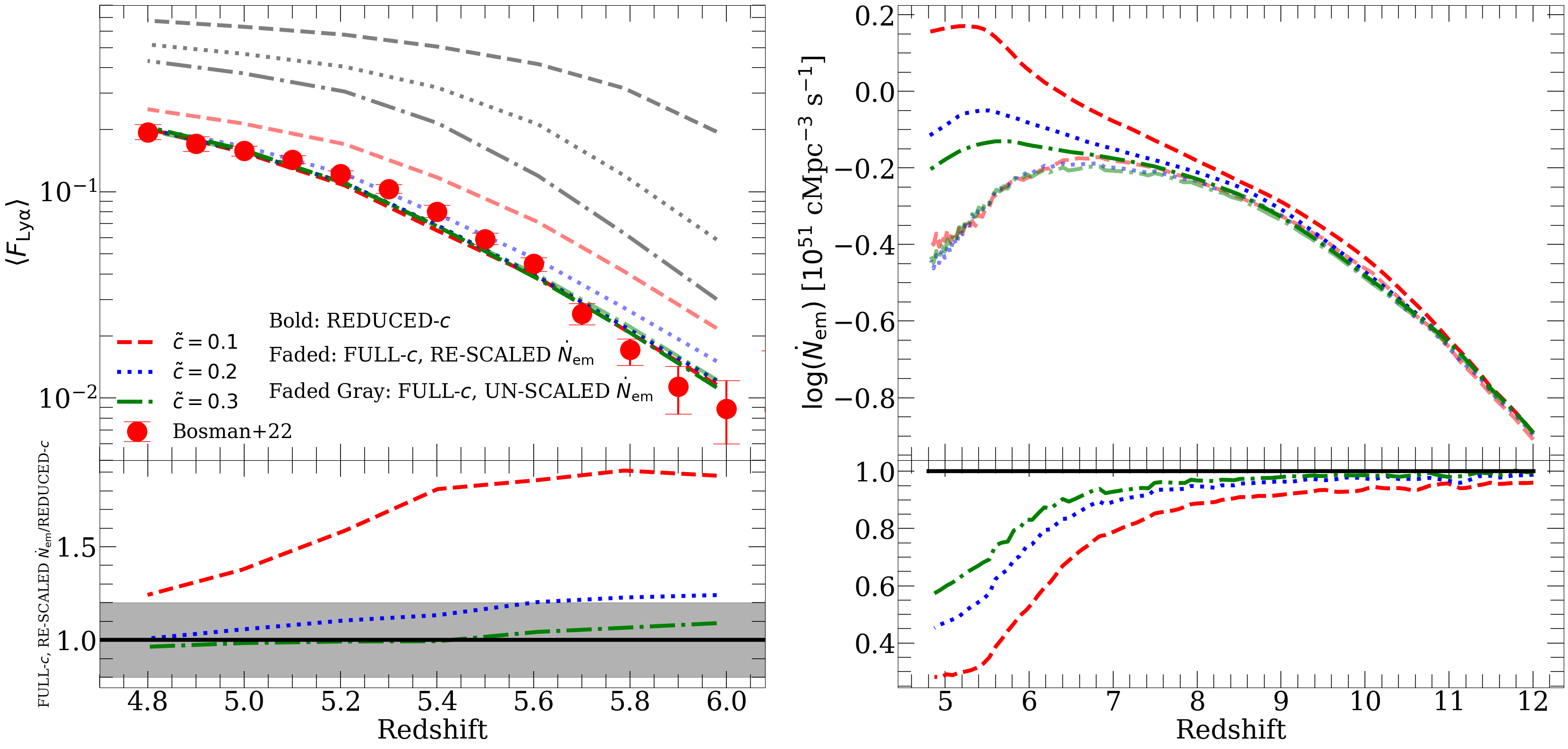
Figure 5: Tests with simulations calibrated to match the Ly$\alpha$ forest at $z=6$. Upper Left: $\langle F_{\rm Ly\alpha}\rangle$ vs. redshift for all three types of simulations described in Table 1 for $\tilde{c}=0.1$, $0.2$, and $0.3$. The formatting of the curves is the same used in Figure 4 (see text and legend). By construction, all the reduced-$c$ results agree with each other and the measurements from Ref. [24]. The full-$c$, re-scaled $\dot{N}_{\rm em}$, $\tilde{c}=0.3$ run is indistinguishable from these. The $\tilde{c}=0.2$ run is slightly above the others, but still in reasonable agreement with the measurements. However, the $\tilde{c}=0.1$ run diverges significantly from the measurements. All the full-$c$, un-scaled $\dot{N}_{\rm em}$ have too much transmission, since they end reionization earlier than the reduced-$c$ runs. Bottom Left: ratio of $\langle F_{\rm Ly\alpha}\rangle$ in the full-$c$, re-scaled $\dot{N}_{\rm em}$ and reduced-$c$ runs, with the shaded region denoting $\pm 20\%$. We find $\lesssim 5\%$ agreement for $\tilde{c}=0.3$ and $\lesssim 20\%$ agreement for $\tilde{c}=0.2$, but for $\tilde{c}=0.1$, the simulations disagree by a factor of $1.3-2$. Upper Right: $\dot{N}_{\rm em}$ for the reduced-$c$ (bold curves) and full-$c$, re-scaled $\dot{N}_{\rm em}$ (faded curves) simulations. As previously mentioned, the reduced-$c$ runs have different $\dot{N}_{\rm em}$ since they are all separately calibrated to match the forest. The full-$c$, re-scaled $\dot{N}_{\rm em}$ runs have similar $\dot{N}_{\rm em}$, which is expected since they use the full speed of light and are supposed to match the same observable, $\langle F_{\rm Ly\alpha}\rangle$. Bottom Right: ratio of $\dot{N}_{\rm em}$ in the full-$c$, re-scaled $\dot{N}_{\rm em}$ and reduced-$c$ runs. They are similar early in reionization but diverge by up to a factor of $3$ by its end.

We first compare the mean transmission of the Ly$\alpha$ forest, $\langle F_{\rm Ly\alpha}\rangle$, with measurements from Ref. [24] in the top left panel of Figure 5. The bold colored lines show reduced-$c$ runs for $\tilde{c}=0.1$, $0.2$, and $0.3$. Faded colored lines (with matching line styles) show the full-$c$, re-scaled $\dot{N}_{\rm em}$ results, and faded gray lines (again, with matching line styles) show the full-$c$, un-scaled $\dot{N}_{\rm em}$ results. The bottom panel shows the ratios of the full-$c$, re-scaled $\dot{N}_{\rm em}$ and reduced-$c$ results (with the shaded line again denoting $\pm 20\%$ from unity). All the reduced-$c$ results agree well with the measurements and each other by construction. The full-$c$, re-scaled $\dot{N}_{\rm em}$ run with $\tilde{c}=0.3$ is indistinguishable from its reduced-$c$ counterpart. For $\tilde{c}=0.2$, $\langle F_{\rm Ly\alpha}\rangle$ for the full-$c$, re-scaled $\dot{N}_{\rm em}$ run slightly above the measurements, but is still within at most $25\%$ of its reduced-$c$ counterpart. However, for $\tilde{c}=0.1$, the full-$c$, re-scaled $\dot{N}_{\rm em}$ run diverges by as much as a factor of $2$. All three of the full-$c$, un-scaled $\dot{N}_{\rm em}$ lie well above the measurements, since their reionization histories end too early.

In the upper right panel, we show the emissivities for the reduced-$c$ and full-$c$, re-scaled $\dot{N}_{\rm em}$ runs ($\dot{N}_{\rm em}^{\tilde{c}}$ and $\dot{N}_{\rm em}^{c}$, respectively). The bottom panel shows their ratio. We see that $\dot{N}_{\rm em}^{\tilde{c}}$ is quite different for different values of $\tilde{c}$, since all runs were calibrated to agree with the same observable. On the other hand, $\dot{N}_{\rm em}^{c}$ is quite similar between the different values of $\tilde{c}$. This is indeed to be expected if Eq. 2.11 is accurate, since each $\dot{N}_{\rm em}^{c}$ is supposed to match the same observable, $\langle F_{\rm Ly\alpha}\rangle$, with the full speed of light. In the lower right panel, we see that the $\dot{N}_{\rm em}^{c}$ and $\dot{N}_{\rm em}^{\tilde{c}}$ are similar early in reionization, but differ by a factor of $2-3$ by its end.

In Figure 6, we make the same comparison for the lyman limit mean free path ($\lambda_{912}^{\rm mfp}$, MFP, left) and the IGM temperature at mean density $T_{0}$ (right). To avoid cluttering the plot, we omit results from the full-$c$, un-scaled $\dot{N}_{\rm em}$ runs. We also include several sets of observations for comparison (see references in caption). For $\tilde{c}=0.2$ and $0.3$, the reduced-$c$ and full-$c$, re-scaled $\dot{N}_{\rm em}$ agree to within a few percent in both $\lambda_{\rm mfp}^{912}$ and $T_{0}$, as the bottom panels show. For $\tilde{c}=0.1$, the disagreement is much larger - up to $35\%$ for $\lambda_{\rm mfp}^{912}$ and $\approx 6\%$ for $T_{0}$. Thus, the trend here is qualitatively similar to that observed in Figures 4 and 5 - namely, that Eq. 2.11 gives a reasonable match between reduced-$c$ and full-$c$, re-scaled $\dot{N}_{\rm em}$ simulations for $\tilde{c}=0.2$, but not for $\tilde{c}=0.1$. This further confirms that our approach can only be reliably used down to $\tilde{c}=0.2$.

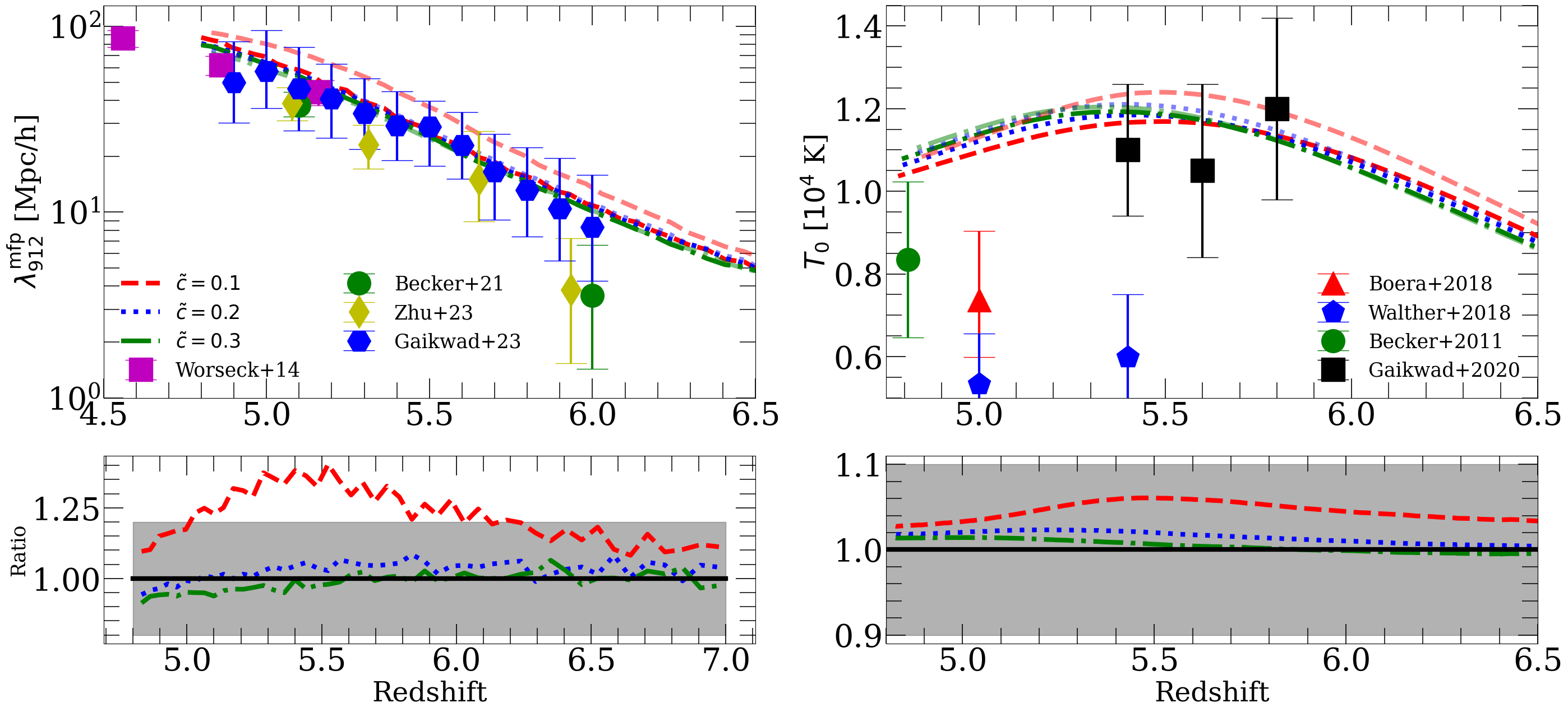
Figure 6: The same as Figure 5, but showing $\lambda_{\rm mfp}^{912}$ (left) and $T_{0}$ (right). To avoid cluttering the plot, we omit the full-$c$, un-scaled $\dot{N}_{\rm em}$ results. For both $\tilde{c}=0.3$ and $0.2$, we see agreement to within a few percent in both quantities between the reduced-$c$ and full-$c$, re-scaled $\dot{N}_{\rm em}$ runs. However, for $\tilde{c}=0.1$, two diverge by up to $\approx 35\%$ for $\lambda_{\rm mfp}^{912}$ and $\approx 6\%$ for $T_{0}$. These results further confirm our earlier observations that our method should only be applied for $\tilde{c}\geq 0.2$.

4.3.2 Large-scale fluctuations

We saw in §4.2.2 and §4.3.1 that the applicability of Eq. 2.11 is likely limited to $\tilde{c}\gtrsim 0.2$ by spatially-varying time-delay effects caused by the RSLA on large scales. In this section, we study this effect in more detail in the context of the Ly$\alpha$ forest. At the end of reionization, large-scale fluctuations in forest properties are set by three quantities that the RSLA affects: the ionization morphology [3], large-scale fluctuations in $\Gamma_{\rm HI}$ [44], and fluctuations in temperature [45]. We will focus on the latter two in this section.

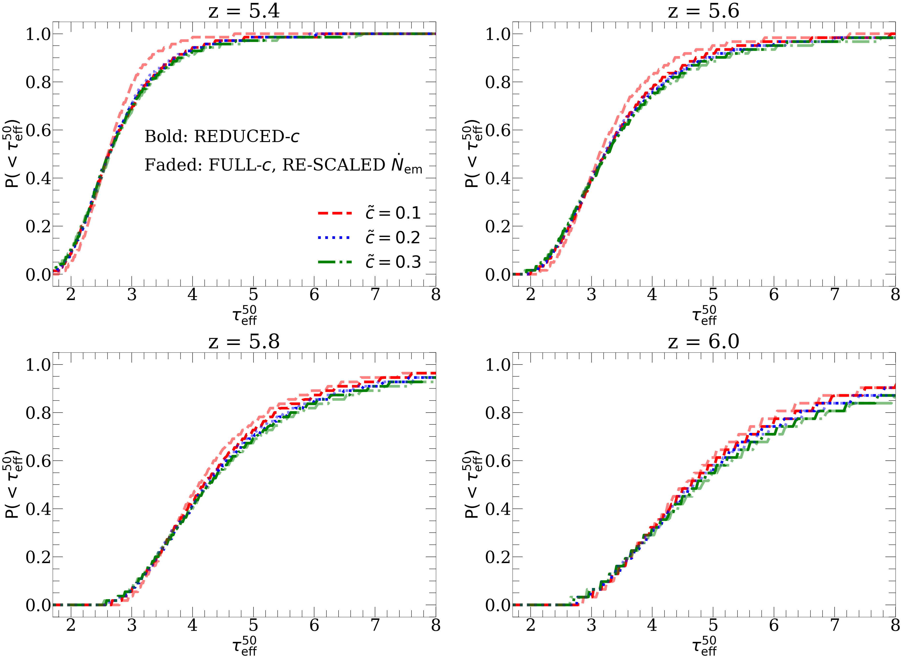
Figure 7: Distribution of Ly$\alpha$ forest effective optical depths over $50$ $h^{-1}$Mpc segments of the forest, $P(<\tau_{\rm eff}^{50})$, at $z=5.4$, $5.6$, $5.8$, and $6.0$. The line styles and colors have the same meanings as in Figure 6. At $z=5.8$ and $6$, when the neutral fraction is $>10\%$, the reduced-$c$ results differ from each other at the few percent level. This is unsurprising since, as we showed earlier, they differ in large-scale ionization morphology. The $\tilde{c}=0.2$ and $0.3$ full-$c$, re-scaled $\dot{N}_{\rm em}$ agree with their reduced-$c$ counterparts to within a few percent, but this deviation grows noticeably larger for $\tilde{c}=0.1$, especially at $z=5.4$ and $5.6$. This suggests that the effect of the RSLA on fluctuations in $\Gamma_{\rm HI}$ and $T$ may be affecting these differences when the neutral fraction is $<10\%$.

In Figure 7, we show the cumulative distribution function (CDF) of $\tau_{\rm eff}^{50}$, $P(<\tau_{\rm eff}^{50})$, the effective optical depth over $50$ $h^{-1}$Mpc segments of the forest, at $z=5.4$, $5.6$, and $5.8$, and $6.0$. This statistic has been used in a number of works to argue that reionization must have ended later than $z=6$ [3, 6, 42, 37, 46, 30]. The format of the curves is the same as that in Figure 6. All the reduced-$c$ runs, and the full-$c$, re-scaled $\dot{N}_{\rm em}$ runs with $\tilde{c}=0.2$ and $0.3$ (faded blue-dotted and green dot-dashed curves) mutually agree to within a few percent at all redshifts. We do see few-percent level differences between different reduced-$c$ runs at $z=6$ and $5.8$, which get smaller at $z=5.6$ and $5.4$. This is unsurprising, since we have already shown that the reduced-$c$ runs differ from each other in large-scale ionization morphology (Figures 3-4), which also affects the $\tau_{\rm eff}^{50}$ CDF when the IGM is still partially neutral. We also see that the full-$c$, re-scaled $\dot{N}_{\rm em}$ $\tilde{c}=0.1$ run differs significantly from the others, especially at $z=5.6$ and $5.4$, when the neutral fraction is $<10\%$. This suggests that the effect of the RSLA on large-scale fluctuations in $\Gamma_{\rm HI}$ and/or $T$ may also play a significant role in driving these differences.

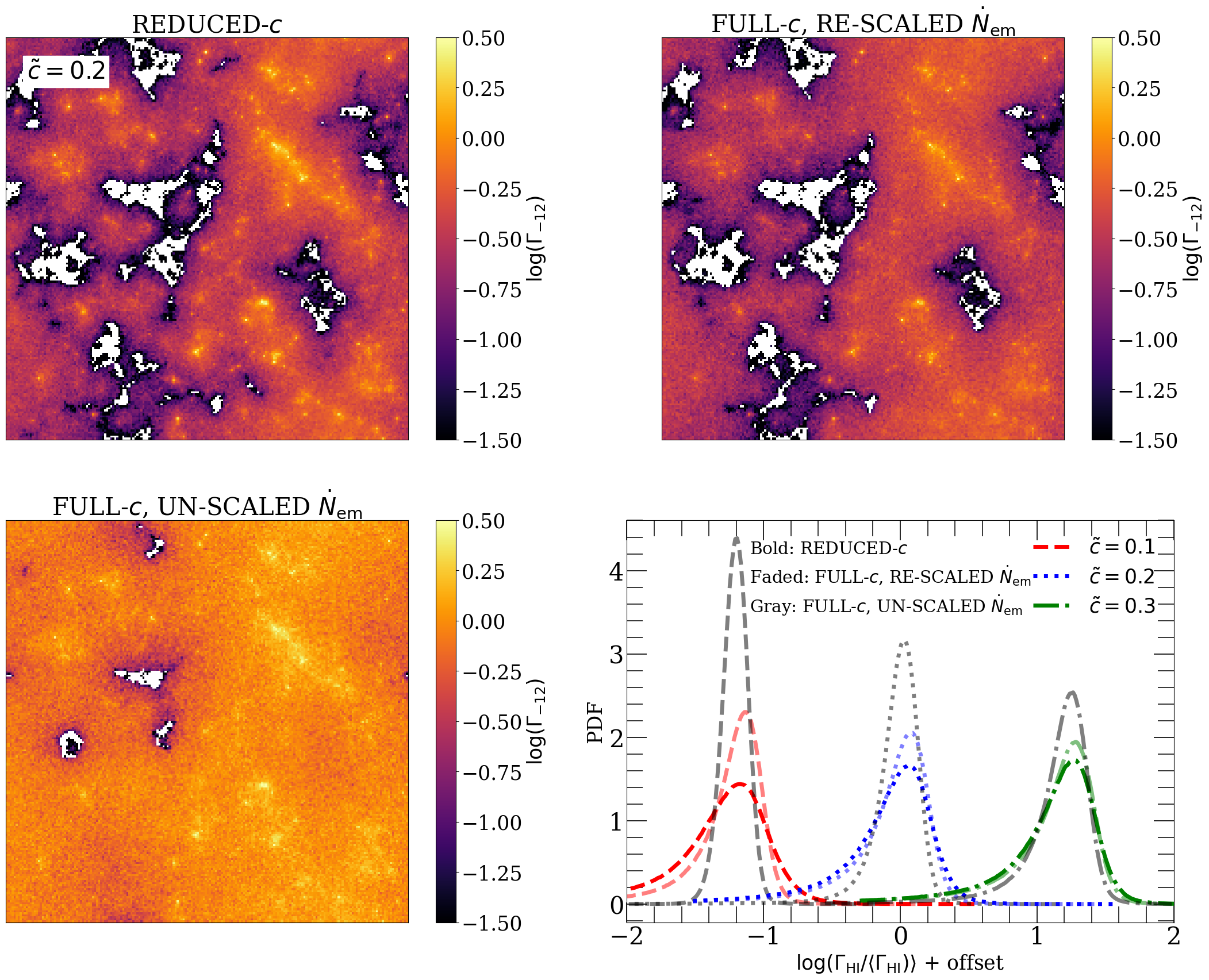
Figure 8: Visualization of the effect of the RSLA on large-scale fluctuations in $\Gamma_{\rm HI}$ (in units of $10^{-12}$ s^-1). We show maps of the reduced-$c$, full-$c$, re-scaled $\dot{N}_{\rm em}$, and full-$c$, un-scaled $\dot{N}_{\rm em}$ runs in the upper left, upper right, and lower left panels, respectively, for $\tilde{c}=0.2$. The full-$c$, un-scaled $\dot{N}_{\rm em}$ run has a higher mean $\Gamma_{\rm HI}$, fewer neutral islands (white regions), and weaker spatial fluctuations in $\Gamma_{\rm HI}$, since reionization ends earlier in that run than in the others. The reduced-$c$ and full-$c$, re-scaled $\dot{N}_{\rm em}$ runs are in reasonably good visual agreement. However, the former has noticeably larger $\Gamma_{\rm HI}$ fluctuations, with the bright (faint) regions being brighter (fainter) than in the full-$c$, re-scaled $\dot{N}_{\rm em}$ run. In the lower right, we plot log-space PDFs of $\Gamma_{\rm HI}$ normalized by its mean. We show results for all three values of $\tilde{c}$, with the same line styles and colors used in Figure 5. We have offset the $\tilde{c}=0.1$ ($0.3$) PDFs by $1.2$ dex to the left (right) for clarity. In all three cases, the PDFs are much narrower in the full-$c$, un-scaled $\dot{N}_{\rm em}$ runs than in the others. As $\tilde{c}$ decreases, the PDFs in the reduced-$c$ become grow wider than their full-$c$, re-scaled $\dot{N}_{\rm em}$ counterparts, owing to time-delay effects (see text).

We visualize the effect of the RSLA on large-scale fluctuations in $\Gamma_{\rm HI}$ in Figure 8. We show maps of $\Gamma_{\rm HI}$ (in units of $10^{-12}$ s^-1) at $z=5.65$, when the universe is $\approx 10\%$ neutral in the reduced-$c$ and full-$c$, re-scaled $\dot{N}_{\rm em}$ runs. The top left, top right, and lower left panels show maps for the reduced-$c$, full-$c$, re-scaled $\dot{N}_{\rm em}$, and full-$c$, un-scaled $\dot{N}_{\rm em}$ runs, respectively, for $\tilde{c}=0.2$. We see that the full-$c$, un-scaled $\dot{N}_{\rm em}$ run has a much higher mean $\Gamma_{\rm HI}$ and weaker $\Gamma_{\rm HI}$ fluctuations than the other two, owing to its earlier end to reionization. Compared to this run, the reduced-$c$ and full-$c$, re-scaled $\dot{N}_{\rm em}$ runs are in relatively good agreement. However, the spatial fluctuations in $\Gamma_{\rm HI}$ are noticeably stronger in the reduced-$c$ run. Once again, this is due to time-delay effects caused by the RSLA. Because photons are delayed longest in reaching the edges of the largest ionized regions, the differences in $N_{\gamma}$ between them and the smaller bubbles are amplified. In addition, photons far from sources were emitted at a retarded time $t_{\rm ret}=R/\tilde{c}$, where $R$ is the ionized bubble size. Again, these effects are accounted for only on average by the re-scaling of Eq. 2.11, which results in larger spatial $\Gamma_{\rm HI}$ fluctuations in the reduced-$c$ runs than in their full-$c$, re-scaled $\dot{N}_{\rm em}$ counterparts.

In the lower right panel, we show the PDFs of $\Gamma_{\rm HI}$, normalized by its mean (in log space). Here, we show results for all three values of $\tilde{c}$, using the same color and line style convention adopted in Figure 5. To make the plot readable, we have offset the $\tilde{c}=0.1$ ($0.3$) PDFs to the left (right) by $1.2$ dex. In all cases, the gray curves are much narrower than the others, reflecting the reduced $\Gamma_{\rm HI}$ fluctuations in the full-$c$, un-scaled $\dot{N}_{\rm em}$ runs. As $\tilde{c}$ decreases, the PDFs of the reduced-$c$ runs grow noticeably wider than those of their full-$c$, re-scaled $\dot{N}_{\rm em}$ counterparts, with the difference becoming very significant for $\tilde{c}=0.1$. These differences contribute to those in $P(<\tau_{\rm eff}^{50})$ seen in Figure 7.

Figure 9 shows the same thing as Figure 8, but for IGM temperature. In the lower right panel, we offset the $\tilde{c}=0.1$ and $0.3$ results by $\pm 30000$ K for clarity. The voids, which have ionized most recently, are hottest in the full-$c$, un-scaled $\dot{N}_{\rm em}$ run, which ends reionization the earliest and most rapidly. The reduced-$c$ run displays the smallest such $T$ enhancements. The fastest I-fronts around the largest ionized regions, which produce the largest $T_{\rm reion}$ [17, 47], grow move more slowly than they should in the reduced-$c$ runs for aforementioned reasons. We see in the lower right panel that the difference between the reduced-$c$ and full-$c$, re-scaled $\dot{N}_{\rm em}$ in the high-$T$ tail of the PDF becomes significant for $\tilde{c}=0.1$, explaining the corresponding differences in $T_{0}$ in Figure 6.

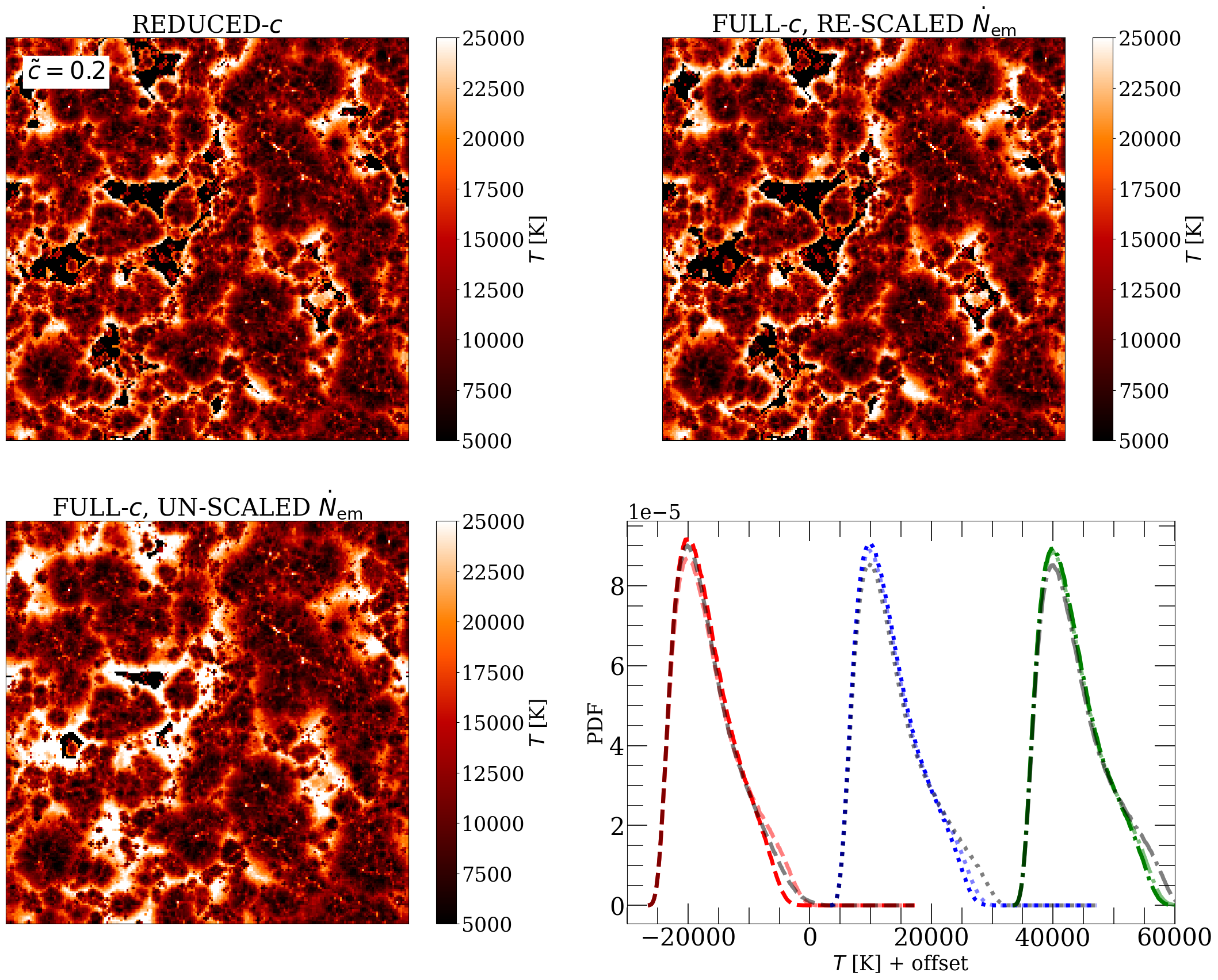
Figure 9: The same as Figure 8, but for the IGM gas temperature. The main difference between the three maps is the strength of the temperature enhancements near neutral islands, where gas has been recently reionized and is hottest. The full-$c$, un-scaled $\dot{N}_{\rm em}$ run has the hottest temperatures in the voids, since reionization ends earliest and most rapidly. The reduced-$c$ run, by contrast, has the weakest $T$ fluctuations. This is because the slowed growth of the largest ionized regions (see §4.2.2) reduces the speed of the fastest I-fronts, which lowers $T_{\rm reion}$ around the largest bubbles. In the lower right panel, we see a significant difference between reduced-$c$ and full-$c$, re-scaled $\dot{N}_{\rm em}$ runs for $\tilde{c}=0.1$ at the high-$T$ end of the PDF, which explains the differences in $T_{0}$ seen in Figure 6.

We have repeated the tests in this section, in whole or in part, for several variations of the properties of the ionized sources and the IGM assumed in this work. We have first varied the clustering of ionizing sources assumed in our fiducial scenario, which assumes that the ionizing emissivity of halos scales with their UV luminosity. We have tested models wherein the bulk of the ionizing photons are emitted by the only the least massive (least clustered) and most massive (most clustered) halos. We have also applied our method to multi-frequency RT simulations, for which we show results in the next section. Lastly, we tested models that assume more sub-grid recombinations than the Reference model of Ref. [23], and we have varied the reionization history. We find that our results remain essentially the same for all of these variations of our fiducial scenario - namely, that Eq. 2.11 is accurate (to $20\%$ or better) for $\tilde{c}=0.2$, but that using $\tilde{c}=0.1$ leads to much larger errors.

These results further corroborate our conclusions from §4.2. We find that, for $\tilde{c}\geq 0.2$, reduced-$c$ simulations calibrated to match the Ly$\alpha$ forest match well the properties of their full-$c$, re-scaled $\dot{N}_{\rm em}$ counterparts. This confirms that Eq. 2.11 can be applied to simulations using the RSLA with $\tilde{c}\geq 0.2$. However, for $\tilde{c}=0.1$, we see significant differences between the reduced-$c$ and full-$c$, re-scaled $\dot{N}_{\rm em}$ runs. These can largely be attributed to position-dependent time-delay effects that arise from using a reduced speed of light, for which Eq. 2.11 does not account. As such, for applications in which the morphology of reionization and/or quasar-based observables at $z\leq 6$ are important, we caution against applying our re-scaling method for $\tilde{c}$ smaller than $0.2$.

5 Generalization to multi-frequency simulations

In the previous section, we tested Eq. 2.11 in mono-chromatic simulations. Here, we will generalize Eq. 2.11 to apply to multi-frequency simulations and demonstrate that the method works just as well in this case, but with one key additional caveat. For our purposes, the main effect of including multi-frequency RT is to change the temperature and ionizing background in the ionized IGM [23], but not the morphology of ionized regions. As such, we will only show our Ly$\alpha$ forest-focused tests (§4.3) in this section.

A straightforward multi-frequency generalization of Eq. 2.11 is to simply apply the arguments of §2.2 in each frequency bin separately. Then we have

$$\dot{N}_{\rm em}^{c}(t,\nu)=\dot{N}_{\rm em}^{\tilde{c}}(t,\nu)-\dot{N}_{\gamma}^{\tilde{c}}(t,\nu)\left(1-\frac{\tilde{c}}{c}\right)$$ (5.1)

A subtlety of Eq. 5.1 is that in general, $\dot{N}_{\rm em}^{\tilde{c}}(t,\nu)$ and $\dot{N}_{\gamma}^{\tilde{c}}(t,\nu)$ do not share the same shape in frequency space. Indeed, this is the case during reionization because the absorption cross-section of HI is frequency-dependent, which results in hardening of the radiation field by the IGM. As such $\dot{N}_{\rm em}^{c}(t,\nu)$ will have a softer ionizing spectrum than $\dot{N}_{\rm em}^{\tilde{c}}(t,\nu)$, since $\dot{N}_{\gamma}^{\tilde{c}}(t,\nu)$ has a harder spectrum. This complicates somewhat the physical interpretation of the re-scaling.

In this section, we use the same setup used for multi-frequency RT simulations described in Ref. [23], assuming that the intrinsic spectrum of ionizing sources is a power law of the form $J_{\nu}\propto\nu^{-\alpha}$ with $\alpha=1.5$. We use $5$ frequency bins, with central frequencies chosen such that (initially) all bins contain an equal fraction of the emitted ionizing photons. The condition for choosing the frequency bins is that the average HI-ionizing cross-section, $\overline{\sigma_{\rm HI}}$, should be the same as that of an $\alpha=1.5$ power law. As in the previous section, we ran reduced-$c$ simulations with $\tilde{c}=0.1$, $0.2$, and $0.3$, and we apply Eq. 5.1 to run their full-$c$, re-scaled $\dot{N}_{\rm em}$ counterparts. In Figure 10, we show $\langle F_{\rm Ly\alpha}\rangle$ in the same format as Figure 5 for our multi-frequency tests, except that we omit the full-$c$, un-scaled $\dot{N}_{\rm em}$ results. We find results very similar to those in Figure 5. The mean flux in the reduced-$c$ and full-$c$, re-scaled $\dot{N}_{\rm em}$ runs remains within $10\%$ for $\tilde{c}=0.3$, and within $30\%$ or better for $\tilde{c}=0.2$. For $\tilde{c}=0.1$, we again find differences as large as a factor of $2$ in $\langle F_{\rm Ly\alpha}\rangle$. In the right column, we see that $\dot{N}_{\rm em}^{\tilde{c}}$ and $\dot{N}_{\rm em}^{c}$, and the relationship between them, are very similar in the multi-frequency runs as in the mono-chromatic case. This shows that our method works just as well when applied to multi-frequency simulations with respect to the mean Ly$\alpha$ forest transmission.

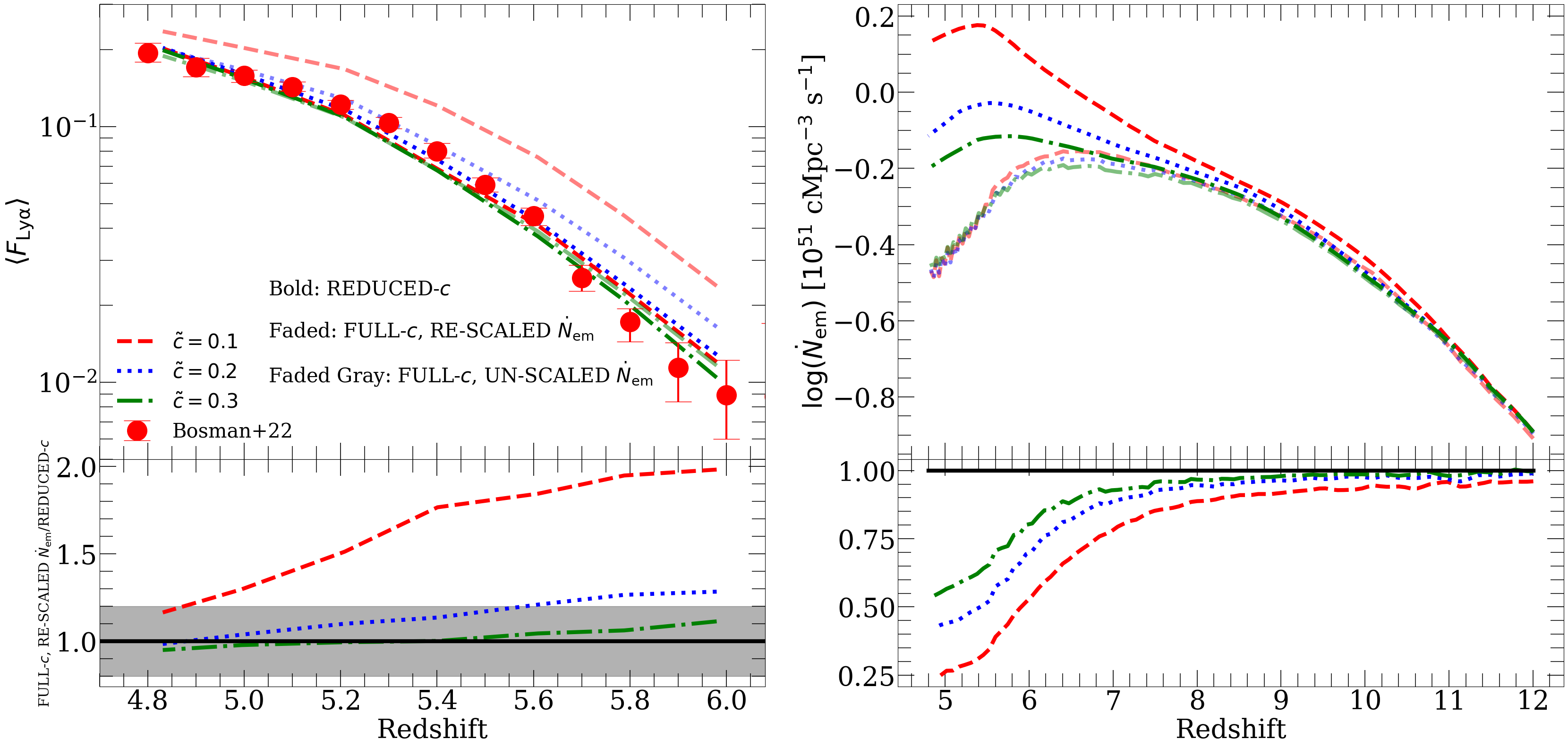
Figure 10: Same as Figure 5, but showing results for our tests with multi-frequency RT, using Eq. 5.1 to re-scale the emissivity. We find very similar results in all panels to those in Figure 5, showing that our method works nearly as well for multi-frequency RT simulations as for single-frequency ones. See text for details.

In Figure 11, we show $P(<\tau_{\rm eff}^{50})$, in the same format as Figure 7, for our multi-frequency tests. Again, we see results very similar to those in Figure 7. The differences between the bold and faded red curves are slightly larger than they are in Figure 7, suggesting that spatial fluctuations in the spectrum of the ionizing background may be slightly worsening the time-delay effects discussed in §4.3.2. However, this effect is not significant enough to change the level of accuracy obtained with $\tilde{c}=0.2$ and $0.3$, further validating that for these values of $\tilde{c}$, our method can safely be applied to simulations with multi-frequency RT.

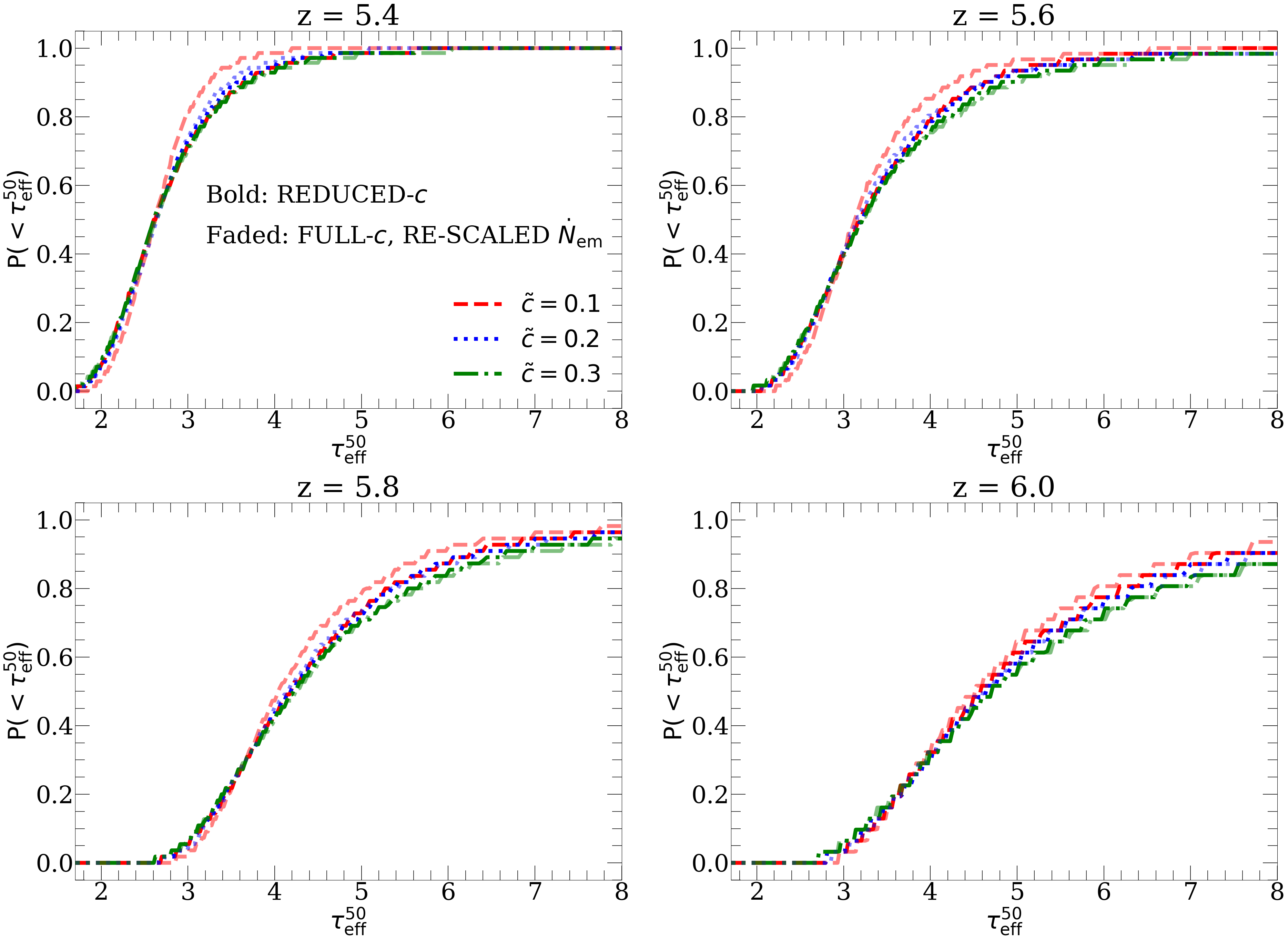
Figure 11: Same as Figure 7, but showing $P(<\tau_{\rm eff}^{50})$ for our multi-frequency RT tests. We find results very similar to those of the mono-chromatic runs, showing that our re-scaling procedure works well in the multi-frequency case. See text for details.

As mentioned, applying Eq. 5.1 in each frequency bin results in $\dot{N}_{\rm em}^{c}(\nu)$ having a different spectral shape than $\dot{N}_{\rm em}^{\tilde{c}}(\nu)$, in a way that depends on redshift. We illustrate this in Figure 12, where we quantify the spectral shape of $\dot{N}_{\rm em}$ before and after the re-scaling. The black solid curve in the left panel shows the fraction of the total emissivity in each bin in our multi-frequency reduced-$c$ run with $\tilde{c}=0.2$ (recall that all bins share the same fraction of the photons in this case). In the right panel, the black dotted curve shows $\frac{1}{N_{\rm freq}}\dot{N}_{\rm em}^{c}$, the fraction that would be in each bin if $\dot{N}_{\rm em}^{c}$ and $\dot{N}_{\rm em}^{\tilde{c}}$ shared the same frequency dependence. The colored dot-dashed lines show $\dot{N}_{\rm em}^{c}(\nu)$ for each bin, with redder (bluer) colors denoting lower (higher) photon energies (see annotations). The re-scaling removes significantly more photons at higher energies, causing $\dot{N}_{\rm em}^{c}(\nu)$ to get softer with decreasing redshift.

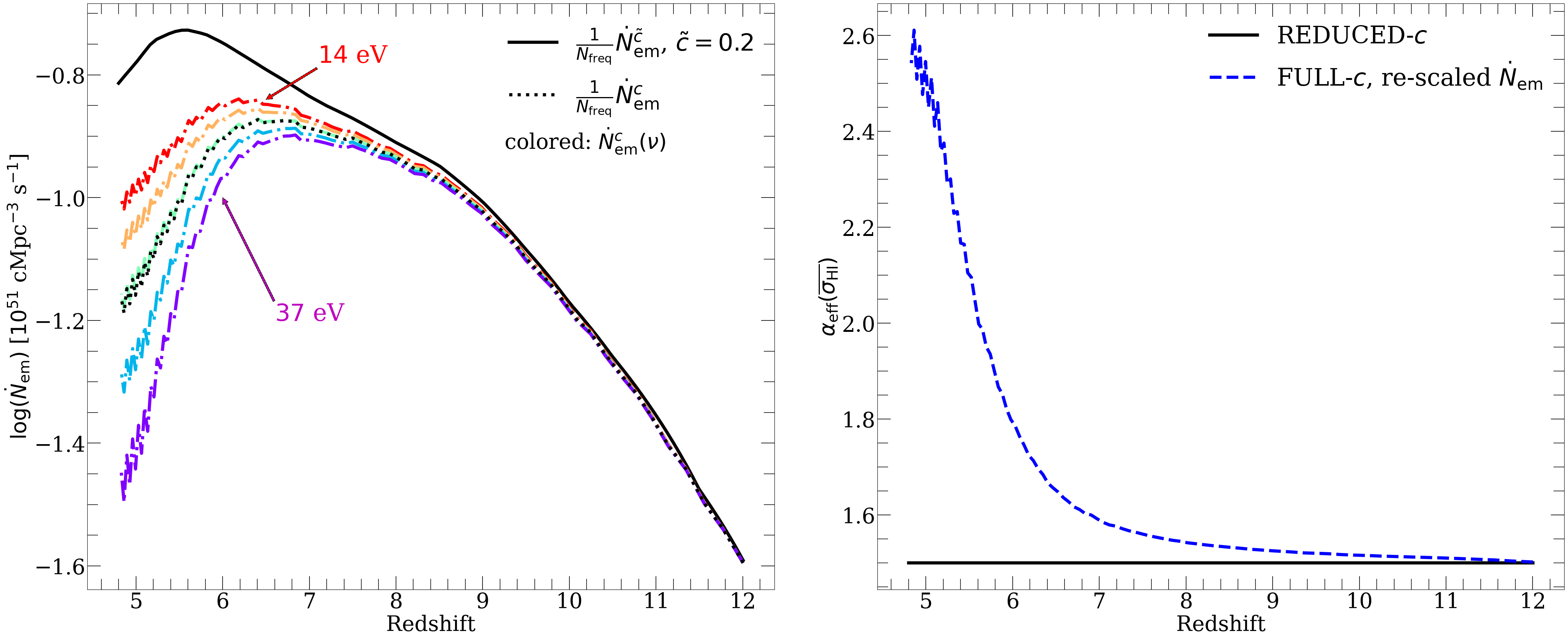
Figure 12: Illustration of how our re-scaling procedure changes the intrinsic spectrum of the sources when applied to multi-frequency RT simulations. Left: Ionizing emissivity in each bin in the reduced-$c$ run (black solid) compared to the spectrum in the full-$c$, re-scaled $\dot{N}_{\rm em}$ run. The black dotted line shows the average fraction of photons in each bin in the latter, while the colored dot-dashed lines show the actual fraction in each of the $5$ frequency bins after re-scaling. Redder (bluer) lines indicate lower (higher) photon energies, as the annotations indicate. The re-scaling removes more high-energy photons from $\dot{N}_{\rm em}^{c}$ due to IGM filtering. Right: effective spectral index $\alpha_{\rm eff}$ (see text) for the multi-frequency reduced-$c$ and full-$c$, re-scaled $\dot{N}_{\rm em}$ simulations. The latter has a softer spectrum (larger $\alpha_{\rm eff}$) which gets softer with time, reaching $2.5$ by $z=5$.

In the right panel, we calculate the “effective” power law index, $\alpha_{\rm eff}$, for each case vs. redshift. We define $\alpha_{\rm eff}$ such that a power law spectrum with that index would have the same $\overline{\sigma_{\rm HI}}$ as the source spectrum in the simulation. For the reduced-$c$ run, this is trivially $1.5$, but for the full-$c$, re-scaled $\dot{N}_{\rm em}$ run, $\alpha_{\rm eff}$ increases with time, reaching $\approx 2.5$ by $z=5$. Note that this effect arises from the fact that the IGM absorbs (filters) low-energy photons more readily than high-energy ones, such that $\dot{N}_{\gamma}$ has a harder spectrum than $\dot{N}_{\rm em}$. This effect will thus be less significant in simulations with less filtering. We showed in Appendix B of Ref. [23] that our simulations are likely predict levels of filtering on the high end of expectations, so the effect may be somewhat exaggerated here. Still, it represents a complication to applying Eq. 5.1 to multi-frequency simulations that should be carefully considered and quantified in any studies that use this approach.

6 Conclusions

In this work, we have studied the effect of the reduced speed of light approximation (RSLA) on radiative transfer simulations of reionization. We used a simple analytic model to show (1) when and why the RSLA produces inaccurate results, especially near reionization’s end, and (2) that using the RSLA is, to a good approximation, equivalent to a redshift-dependent re-scaling of the global ionizing emissivity of reionization’s sources (Eq. 2.11). We have run simulations with the reduced speed of light (reduced-$c$ runs) and with the full speed of light after applying the re-scaling prescribed by Eq. 2.11 (full-$c$, re-scaled $\dot{N}_{\rm em}$ runs). We have assessed how accurate Eq. 2.11 is by comparing these two sets of simulations in a number of different physical properties and observables. Our main findings are summarized below:

• For $\tilde{c}$ as small as $0.05$, our reduced-$c$ and full-$c$, re-scaled $\dot{N}_{\rm em}$ simulations agree in the global reionization history within a linear difference of $\lesssim 0.01$ at all redshifts. This confirms that that the re-scaling of $\dot{N}_{\rm em}$ prescribed by Eq. 2.11 is equivalent to using the RSLA with respect to the global reionization history.

• We have compared the morphology of ionized regions and the 21 cm power spectrum in our reduced-$c$ and full-$c$, re-scaled $\dot{N}_{\rm em}$ runs. We find that the sizes of the largest ionized regions are suppressed in the reduced-$c$ runs relative to their full-$c$, re-scaled $\dot{N}_{\rm em}$ counterparts. This is caused by position-dependent time-delay effects caused by the RSLA for which Eq. 2.11 does not account. The net effect is to suppress ionization power in the reduced-$c$ simulations. We find that differences in the 21 cm power spectrum at $k=0.1$ $h$Mpc^-1 is at most $15\%$ ($10\%$) for $\tilde{c}=0.2$ ($0.3$), but can exceed $20\%$ for $\tilde{c}=0.1$ and $30\%$ for $\tilde{c}=0.05$. As such, we recommend applying Eq. 2.11 only for $\tilde{c}\geq 0.2$ when ionization morphology is important.

• We have made the same comparison with respect to observables derived from high-redshift quasar spectra, with a focus on the Ly$\alpha$ forest at $z\leq 6$. We find that when $\dot{N}_{\rm em}$ is calibrated to reproduce the mean transmission of the Ly$\alpha$ forest at $z\leq 6$, the resulting $\dot{N}_{\rm em}$ histories are very different for different $\tilde{c}$. For reduced-$c$ runs calibrated in this way with $\tilde{c}=0.2$, and $0.3$, we find that their full-$c$, re-scaled $\dot{N}_{\rm em}$ agree in the mean transmission to $20\%$ or better. However, for $\tilde{c}=0.1$ the difference can be as large as a factor of $2$. We find qualitatively similar results for the ionizing photon mean free path and the IGM temperature at mean density. Both agree to within $\leq 5\%$ for $\tilde{c}=0.2$ and $0.3$, but differ by up to $35\%$ and $6\%$, respectively, for $\tilde{c}=0.1$.

• We looked at the large-scale fluctuations in the Ly$\alpha$ forest opacity in our two sets of simulations. For $\tilde{c}\geq 0.2$, the distribution of effective optical depths over $50$ $h^{-1}$Mpc segments of the forest agrees to within a few percent between reduced-$c$ and full-$c$, re-scaled $\dot{N}_{\rm em}$ simulations. Once again, we find that these differences are considerably larger for $\tilde{c}=0.1$. We explored this result in more depth by looking at the large-scale fluctuations in $\Gamma_{\rm HI}$ and $T$ during the end stages of reionization. reduced-$c$ simulations over-produce large-scale fluctuations in $\Gamma_{\rm HI}$ relative to their full-$c$, re-scaled $\dot{N}_{\rm em}$ counterparts thanks to the same position-dependent time-delay effects responsible for affecting the ionization morphology. In addition, reduced-$c$ simulations slightly under-estimate the temperatures of recently ionized, hot voids near reionization’s end, owing to their lower mean I-front speeds.

• Lastly, we generalized our method to apply to multi-frequency RT simulations. We found that with respect to the Ly$\alpha$ forest, the method works just as well with multi-frequency simulations as with single-frequency ones. However, because of IGM filtering effects, $\dot{N}_{\rm em}^{c}$ ends up having a softer spectrum than $\dot{N}_{\rm em}^{\tilde{c}}$, complicating the physical interpretation of the re-scaling procedure. We caution that when applying our method to multi-frequency simulations, this effect should be quantified and its implications carefully considered.

The approach described in this work is potentially useful in the following situations: either (1) when $\dot{N}_{\rm em}$ is entirely a free function of redshift that is calibrated to match some observable (as in Refs. [23, 14]) or (2) when $\dot{N}_{\rm em}$ is uniquely determined by some set of free parameters that are being marginalized over, as in Ref. [30]. In the first case, $\dot{N}_{\rm em}$ can be calibrated using the RSLA at a reduced computational cost, and Eq. 2.11 can be applied to the end result to recover the “true” $\dot{N}_{\rm em}$. In the second case, the re-scaling prescribed by Eq. 2.11 would be equivalent to changing the mapping between $\dot{N}_{\rm em}$ and the free parameters that determine it in a quantifiable way. Unfortunately, our method is not directly applicable for situations where $\dot{N}_{\rm em}$ cannot simply be re-scaled after the simulation has been run. This is the case if $\dot{N}_{\rm em}$ is a self-consistent prediction a model that has no or very few free parameters, such as the THESAN [19, 7], CoDa [13, 5], or SPHINX [48, 49] simulations. Our results further suggest that for the first two applications, the RSLA should only be used (in conjunction with Eq. 2.11/5.1) for $\tilde{c}\geq 0.2$, to ensure that the effects of the RSLA on large-scale fluctuations in the ionization and radiation fields are minimized. This corresponds to a speed-up factor of up to $5$, which will help enable considerably faster searches of the reionization parameter space using RT simulations.

References

- [1] X. Fan, M.A. Strauss, R.H. Becker, R.L. White, J.E. Gunn, G.R. Knapp et al., Constraining the Evolution of the Ionizing Background and the Epoch of Reionization with z~6 Quasars. II. A Sample of 19 Quasars, The Astronomical Journal 132 (2006) 117 [astro-ph/0512082].
- [2] B.E. Robertson, R.S. Ellis, S.R. Furlanetto and J.S. Dunlop, Cosmic Reionization and Early Star-forming Galaxies: A Joint Analysis of New Constraints from Planck and the Hubble Space Telescope, The Astrophysical Journal Letters 802 (2015) L19 [1502.02024].
- [3] G. Kulkarni, L.C. Keating, M.G. Haehnelt, S.E.I. Bosman, E. Puchwein, J. Chardin et al., Large Ly opacity fluctuations and low CMB in models of late reionization with large islands of neutral hydrogen extending to z < 5.5, Monthly Notices of the Royal Astronomical Society 485 (2019) L24 [1809.06374].
- [4] N.Y. Gnedin, Cosmic Reionization on Computers. I. Design and Calibration of Simulations, The Astrophysical Journal 793 (2014) 29 [1403.4245].
- [5] P. Ocvirk, D. Aubert, J.G. Sorce, P.R. Shapiro, N. Deparis, T. Dawoodbhoy et al., Cosmic Dawn II (CoDa II): a new radiation-hydrodynamics simulation of the self-consistent coupling of galaxy formation and reionization, Monthly Notices of the Royal Astronomical Society 496 (2020) 4087 [1811.11192].
- [6] L.C. Keating, L.H. Weinberger, G. Kulkarni, M.G. Haehnelt, J. Chardin and D. Aubert, Long troughs in the Lyman- forest below redshift 6 due to islands of neutral hydrogen, Monthly Notices of the Royal Astronomical Society 491 (2020) 1736 [1905.12640].
- [7] E. Garaldi, R. Kannan, A. Smith, V. Springel, R. Pakmor, M. Vogelsberger et al., The THESAN project: properties of the intergalactic medium and its connection to reionization-era galaxies, Monthly Notices of the Royal Astronomical Society (2022) [2110.01628].
- [8] N.Y. Gnedin and T. Abel, Multi-dimensional cosmological radiative transfer with a Variable Eddington Tensor formalism, New Astronomy 6 (2001) 437 [astro-ph/0106278].
- [9] D. Aubert and R. Teyssier, A radiative transfer scheme for cosmological reionization based on a local Eddington tensor, Monthly Notices of the Royal Astronomical Society 387 (2008) 295 [0709.1544].
- [10] X. Wu, M. McQuinn and D. Eisenstein, On the accuracy of common moment-based radiative transfer methods for simulating reionization, Journal of Cosmology and Astroparticle Physics 2021 (2021) 042 [2009.07278].
- [11] T. Abel and B.D. Wandelt, Adaptive ray tracing for radiative transfer around point sources, Monthly Notices of the Royal Astronomical Society 330 (2002) L53 [astro-ph/0111033].
- [12] H. Trac and R. Cen, Radiative transfer simulations of cosmic reionization. i. methodology and initial results, The Astrophysical Journal 671 (2007) 1.
- [13] P. Ocvirk, N. Gillet, P.R. Shapiro, D. Aubert, I.T. Iliev, R. Teyssier et al., Cosmic Dawn (CoDa): the First Radiation-Hydrodynamics Simulation of Reionization and Galaxy Formation in the Local Universe, Monthly Notices of the Royal Astronomical Society 463 (2016) 1462 [1511.00011].
- [14] S. Asthana, M.G. Haehnelt, G. Kulkarni, D. Aubert, J.S. Bolton and L.C. Keating, Late-end reionization with ATON-HE: towards constraints from Ly emitters observed with JWST, Monthly Notices of the Royal Astronomical Society 533 (2024) 2843 [2404.06548].
- [15] Y. Mao, J. Koda, P.R. Shapiro, I.T. Iliev, G. Mellema, H. Park et al., The impact of inhomogeneous subgrid clumping on cosmic reionization, Monthly Notices of the Royal Astronomical Society 491 (2020) 1600 [1906.02476].
- [16] C. Cain, A. D’Aloisio, N. Gangolli and G.D. Becker, A Short Mean Free Path at z = 6 Favors Late and Rapid Reionization by Faint Galaxies, The Astrophysical Journal Letters 917 (2021) L37 [2105.10511].
- [17] A. D’Aloisio, M. McQuinn, O. Maupin, F.B. Davies, H. Trac, S. Fuller et al., Heating of the Intergalactic Medium by Hydrogen Reionization, The Astrophysical Journal 874 (2019) 154 [1807.09282].
- [18] A. D’Aloisio, M. McQuinn, H. Trac, C. Cain and A. Mesinger, Hydrodynamic response of the intergalactic medium to reionization, The Astrophysical Journal 898 (2020) 149.
- [19] R. Kannan, E. Garaldi, A. Smith, R. Pakmor, V. Springel, M. Vogelsberger et al., Introducing the THESAN project: radiation-magnetohydrodynamic simulations of the epoch of reionization, Monthly Notices of the Royal Astronomical Society 511 (2022) 4005 [2110.00584].
- [20] N.Y. Gnedin, On the Proper Use of the Reduced Speed of Light Approximation, The Astrophysical Journal 833 (2016) 66 [1607.07869].
- [21] N. Deparis, D. Aubert, P. Ocvirk, J. Chardin and J. Lewis, Impact of the reduced speed of light approximation on ionization front velocities in cosmological simulations of the epoch of reionization, Astronomy and Astrophysics 622 (2019) A142 [1803.01634].
- [22] P. Ocvirk, D. Aubert, J. Chardin, N. Deparis and J. Lewis, Impact of the reduced speed of light approximation on the post-overlap neutral hydrogen fraction in numerical simulations of the epoch of reionization, Astronomy and Astrophysics 626 (2019) A77 [1803.02434].
- [23] C. Cain, A. D’Aloisio, G. Lopez, N. Gangolli and J.T. Roth, On the rise and fall of galactic ionizing output at the end of reionization, Monthly Notices of the Royal Astronomical Society 531 (2024) 1951 [2311.13638].
- [24] S.E.I. Bosman, F.B. Davies, G.D. Becker, L.C. Keating, R.L. Davies, Y. Zhu et al., Hydrogen reionization ends by z = 5.3: Lyman- optical depth measured by the XQR-30 sample, Monthly Notices of the Royal Astronomical Society 514 (2022) 55 [2108.03699].
- [25] Planck Collaboration, N. Aghanim, Y. Akrami, M. Ashdown, J. Aumont, C. Baccigalupi et al., Planck 2018 results. VI. Cosmological parameters, Astronomy and Astrophysics 641 (2020) A6 [1807.06209].
- [26] G.D. Becker and J.S. Bolton, New measurements of the ionizing ultraviolet background over 2 < z < 5 and implications for hydrogen reionization, Monthly Notices of the Royal Astronomical Society 436 (2013) 1023 [1307.2259].
- [27] F. Nasir, C. Cain, A. D’Aloisio, N. Gangolli and M. McQuinn, Hydrodynamic Response of the Intergalactic Medium to Reionization. II. Physical Characteristics and Dynamics of Ionizing Photon Sinks, The Astrophysical Journal 923 (2021) 161 [2108.04837].
- [28] T. Theuns and T.K. Chan, A halo model for cosmological Lyman-limit systems, Monthly Notices of the Royal Astronomical Society 527 (2024) 689 [2310.09228].
- [29] A. Mesinger and S. Furlanetto, Efficient Simulations of Early Structure Formation and Reionization, The Astrophysical Journal 669 (2007) 663 [0704.0946].
- [30] Y. Qin, A. Mesinger, S.E.I. Bosman and M. Viel, Reionization and galaxy inference from the high-redshift Ly forest, Monthly Notices of the Royal Astronomical Society 506 (2021) 2390 [https://academic.oup.com/mnras/article-pdf/506/2/2390/39136191/stab1833.pdf].
- [31] C. Cain, A. D’Aloisio, N. Gangolli and M. McQuinn, The morphology of reionization in a dynamically clumpy universe, Monthly Notices of the Royal Astronomical Society 522 (2023) 2047 [2207.11266].
- [32] C. Cain and A. D’Aloisio, FlexRT – A fast and flexible cosmological radiative transfer code for reionization studies I: Code validation, arXiv e-prints (2024) arXiv:2409.04521 [2409.04521].
- [33] S.K. Giri, G. Mellema and R. Ghara, Optimal identification of H II regions during reionization in 21-cm observations, Monthly Notices of the Royal Astronomical Society 479 (2018) 5596 [1801.06550].
- [34] Z. Abdurashidova, J.E. Aguirre, P. Alexander, Z.S. Ali, Y. Balfour, A.P. Beardsley et al., First Results from HERA Phase I: Upper Limits on the Epoch of Reionization 21 cm Power Spectrum, The Astrophysical Journal 925 (2022) 221 [2108.02263].
- [35] Z. Abdurashidova, J.E. Aguirre, P. Alexander, Z.S. Ali, Y. Balfour, R. Barkana et al., HERA Phase I Limits on the Cosmic 21 cm Signal: Constraints on Astrophysics and Cosmology during the Epoch of Reionization, The Astrophysical Journal 924 (2022) 51 [2108.07282].
- [36] L.M. Berkhout, D.C. Jacobs, Z. Abdurashidova, T. Adams, J.E. Aguirre, P. Alexander et al., Hydrogen Epoch of Reionization Array (HERA) Phase II Deployment and Commissioning, Publications of the ASP 136 (2024) 045002 [2401.04304].
- [37] F. Nasir and A. D’Aloisio, Observing the tail of reionization: neutral islands in the z = 5.5 lyman- forest, Monthly Notices of the Royal Astronomical Society 494 (2020) 3080–3094.
- [38] G. Worseck, J.X. Prochaska, J.M. O’Meara, G.D. Becker, S.L. Ellison, S. Lopez et al., The Giant Gemini GMOS survey of zem > 4.4 quasars - I. Measuring the mean free path across cosmic time, Monthly Notices of the Royal Astronomical Society 445 (2014) 1745 [1402.4154].
- [39] G.D. Becker, A. D’Aloisio, H.M. Christenson, Y. Zhu, G. Worseck and J.S. Bolton, The mean free path of ionizing photons at 5 < z < 6: evidence for rapid evolution near reionization, Monthly Notices of the Royal Astronomical Society 508 (2021) 1853 [2103.16610].
- [40] Y. Zhu, G.D. Becker, H.M. Christenson, A. D’Aloisio, S.E.I. Bosman, T. Bakx et al., Probing Ultralate Reionization: Direct Measurements of the Mean Free Path over 5 < z < 6, The Astrophysical Journal 955 (2023) 115 [2308.04614].
- [41] P. Gaikwad, M.G. Haehnelt, F.B. Davies, S.E.I. Bosman, M. Molaro, G. Kulkarni et al., Measuring the photo-ionization rate, neutral fraction and mean free path of HI ionizing photons at from a large sample of XShooter and ESI spectra, arXiv e-prints (2023) arXiv:2304.02038 [2304.02038].
- [42] L.C. Keating, G. Kulkarni, M.G. Haehnelt, J. Chardin and D. Aubert, Constraining the second half of reionization with the Ly forest, Monthly Notices of the Royal Astronomical Society 497 (2020) 906 [1912.05582].
- [43] J. Chardin, M.G. Haehnelt, D. Aubert and E. Puchwein, Calibrating cosmological radiative transfer simulations with Ly forest data: evidence for large spatial UV background fluctuations at z 5.6-5.8 due to rare bright sources, Monthly Notices of the Royal Astronomical Society 453 (2015) 2943 [1505.01853].
- [44] F.B. Davies and S.R. Furlanetto, Large fluctuations in the hydrogen-ionizing background and mean free path following the epoch of reionization, Monthly Notices of the Royal Astronomical Society 460 (2016) 1328 [1509.07131].
- [45] A. D’Aloisio, M. McQuinn and H. Trac, LARGE OPACITY VARIATIONS IN THE HIGH-REDSHIFT LYFOREST: THE SIGNATURE OF RELIC TEMPERATURE FLUCTUATIONS FROM PATCHY REIONIZATION, The Astrophysical Journal 813 (2015) L38.
- [46] T.R. Choudhury, A. Paranjape and S.E.I. Bosman, Studying the Lyman optical depth fluctuations at z 5.5 using fast semi-numerical methods, Monthly Notices of the Royal Astronomical Society 501 (2021) 5782 [2003.08958].
- [47] C. Zeng and C.M. Hirata, Nonequilibrium Temperature Evolution of Ionization Fronts during the Epoch of Reionization, The Astrophysical Journal 906 (2021) 124 [2007.02940].
- [48] J. Rosdahl, H. Katz, J. Blaizot, T. Kimm, L. Michel-Dansac, T. Garel et al., The SPHINX cosmological simulations of the first billion years: the impact of binary stars on reionization, Monthly Notices of the Royal Astronomical Society 479 (2018) 994 [1801.07259].
- [49] H. Katz, S. Martin-Alvarez, J. Rosdahl, T. Kimm, J. Blaizot, M.G. Haehnelt et al., Introducing SPHINX-MHD: the impact of primordial magnetic fields on the first galaxies, reionization, and the global 21-cm signal, Monthly Notices of the Royal Astronomical Society 507 (2021) 1254 [2101.11624].