History of a Particle Bounded to the Cosmological LTB Black Hole Surrounded by the Quintom Field

Abstract

In this paper, we provide a complete set of analytic time-varying geodesic equations of the LTB black hole surrounded by the Quintom field. Indeed, we probe the evolution of the effective potential of such a black hole and possible photon orbits on cosmic epochs. We deduce that passing time in the accelerated universe from the early to late time epochs causes the peak of effective potential to decrease and shift to small radii, while the possibility of forming a stable orbit increases. Besides, four situations including: terminating bound orbit, stable orbit, scattering flyby orbit, and terminating escape orbit have been illustrated in some cosmic time slices. Moreover, changing orbits with time from the early universe to the late time epochs have been investigated. Furthermore, the stability of orbits and ISCO have been analyzed.

Keywords: Cosmological Black Hole, Dark Energy, Quintom Field, LTB Black Hole, Geodesics Structure.

I Introduction

After discovering both the stationary black hole and the accelerated universe, the issue was raised about considering a black hole in this accelerated universe. Therefore, the subject of cosmological black holes was introduced with this content. The first suggestion for a black hole in the accelerating Friedmann-Robertson-Walker (FRW) universe can be found in McVitie’s research 33McV . Later, other famous solutions have been suggested by Einstein and Strauss 45Ein , Vaidya 77Vai , and Lemaître-Tolman-Bondi (LTB) 34Tol ; 47Bon ; 97Lem . The obvious characteristic of all these solutions is the dynamical component existence such as time in the black hole metric. Therefore, in all solutions, the basic definitions of stationary black holes such as mass, surface gravity, event horizon, etc., have been redefined based on the existence of black holes in a dynamical background 94Hay ; 02Ash ; 14Far . In addition, we notice that each solution answers part of the relevant questions and leaves some ambiguity; in Ref. 15Far , one can find a helpful review on the cosmological black hole. In this research, we pay specific attention to the LTB solution which has been probed in the various research like Refs. 10Fir ; 11Gao ; 11Chak ; 22Kok ; 23Sch . In Ref. 10Fir , authors have introduced the LTB black hole as a collapsing over-dense region extending to an expanding closed, open, or flat asymptotically FRW universe. In Ref. 11Gao , the metric of LTB black hole has been generalized to the LTB black hole in the several backgrounds of a spatially flat, dark matter, dark matter plus dark energy, or dark energy dominated universe. In Ref. 11Chak , three laws of thermodynamics for the inhomogeneous spherically symmetric LTB model has been analyzed. Besides, in Ref. 22Kok , light-rays propagating through the LTB geometrical structure has been investigated. Also, in the newest research in Ref. 23Sch , the evolution of spherical symmetric inhomogeneities of $\Lambda$LTB model has been compared with inhomogeneous cosmological models based on $f(R)$ modified gravity theories.

The most remarkable aspect of the accelerated universe is how the acceleration has been created. On the one hand, the answer of particle physics to this question is the existence of some fields like Quintessence 13Tsu , Phantom 02Cal , K-essence 01Arm , and Tachyon 02Sen as a Dark Energy. On the other hand, observational data illustrate the transition for the value of the equation of state from $w>-1$ at the prior epochs to $w<-1$ at the late epochs of the cosmic time. Therefore, it is undeniable that we pay special attention to the field that expects this transition. It can be considered the combination of two field components like Quintessence and Phantom such that the evolution of kinetic energy of those two fields describes $w$ crosses $-1$. Such a field is named Quintom which has been considered in recent research 04Eliz ; 05Fen ; 08Noz ; 10Set ; 16Noz . Also, Ref. 08Eli provides a helpful demonstration of the universe’s history by comparing single or multiple scalar field theories. Therefore, we can interpret that there are cosmological LTB black holes surrounded by the field that accelerates the universe. Likewise, Refs. 11Gao ; 08Gao ; 17Lei ; 23Far can be mentioned as instance research in this issue. Moreover, we are also interested in other aspects of the massive objects in the accelerated universe such as the geodesics of spacetime which can provide a perfect understanding of the motion of light rays in all time cosmic epochs. Indeed, attention to the geodesics equation of a gravitational field is an essential feature for predicting observational effects like gravitational time delay, light deflection, and perihelion shift. In this regard, we have provided a comprehensive investigation of the geodesics and possible orbits in Refs. 15Sor ; 16Sor ; 22Sor . Especially, in Ref. 16Sor , we have probed in the geodesics of the Kerr-Newman-AdS spacetime numerically. As well, in Ref. 22Sor , we have done the analytical research on the black hole immersed in dust, radiation, cosmological constant, and Phantom field, separately. Besides, it has been investigated in Refs. 14Nol ; 16Ant for the McVitie black hole as a cosmological black hole. Also, in Ref. 02Bak , applying the Lemaître-Schwarzschild solution, the author has achieved domains of attraction for some local structures like the Milky Way or Virgo Cluster. In addition, authors in Ref. 04Nes have done interesting numerical research about bound systems like the Milky Way in the universes with accelerating expansion either increases with time for phantom cosmologies or decreases with time for quintessence.

In this paper, we review the cosmological LTB black hole surrounded by the Quintom field in Section II. Afterward, we investigate the effective potential and photon orbit for a particle bounded to such a black hole in the accelerated universe with Quintom content in section III. We provide discussion and conclusion in final section.

II Outlook on the Cosmological LTB Black Hole with the Quintom field as a Content of the Universe

Cosmological LTB black hole was introduced by Lemaître, then it was investigated by Tolman and Bondi. So, such a black hole in the FRW universe has formed entitled LTB black hole 00Cel with the line element as the form below

$$ds^{2}=-dt^{2}+\frac{R^{\prime 2}(r,t)}{1+2E(r)}dr^{2}+R^{2}(r,t)(d\theta^{2}+\sin^{2}\theta d\varphi^{2}).$$ (1)

In this metric, $R(r,t)$ is a physical radius and,

$$E(r)=\frac{1}{2}\dot{R}^{2}(r,t)-\frac{M(R)}{R(r,t)},$$ (2)

is the interpretation of the total energy per unit mass, where $M(R)$ could be Misner-Sharp mass as follows

$$M_{M-Sh}=M+\frac{4\pi}{3}\rho R^{3}.$$ (3)

Also, we notice that hereafter overdot and prime denote differentiation with respect to $t$ and $r$, respectively. Afterwards, one can considers a perfect fluid like Quintom as a content of the universe with the energy-momentum tensor as follows

$$T_{\mu\nu}=(\rho+p)u_{\mu}u_{\nu}+pg_{\mu\nu},$$ (4)

where $\rho$ and $p$ are density and pressure of the Quintom field, respectively; and $u^{\mu}=(1,0,0,0)$ is the four-velocity. The Quintom field has been made of these two field compositions 05Fen ; 10Set . So that, the equation of state has been written as follows

$$w_{q}=\frac{\frac{1}{2}\dot{\delta}^{2}-V_{\delta}(\delta)-\frac{1}{2}\dot{\sigma}^{2}-V_{\sigma}(\sigma)}{\frac{1}{2}\dot{\delta}^{2}+V_{\delta}(\delta)-\frac{1}{2}\dot{\sigma}^{2}+V_{\sigma}(\sigma)},$$ (5)

where $V_{\delta}(\delta)$ and $V_{\sigma}(\sigma)$ are the potentials for the canonical Quintessence and the Phantom field, respectively. Therefore, it is easy to conclude that the equation of state for the Quintom field crosses $-1$ in the near past because the difference in kinetic energy between the two fields evolves. Afterward, to reconstruct the LTB black hole surrounded by the Quintom field, we take on the general line element as the form

$$ds^{2}=-dt^{2}+e^{\bar{\phi}(t,r)}dr^{2}+e^{\phi(t,r)}(d\theta^{2}+\sin^{2}\theta\leavevmode\nobreak\ d\varphi^{2}),$$ (6)

where $t$ is a cosmic time parameter and $(r,\theta,\varphi)$ are co-moving coordinates. The co-moving observer finds a spatially homogeneous pressure since the source is a single perfect fluid and the background is spatially flat 11Gao . Therefore, the pressure has been assumed spatially homogeneous in the form

$$p=-\frac{p_{0}}{(t_{BR}-t)^{2}},$$ (7)

while $p_{0}$ is a positive constant, and $t_{BR}$ is recognized as the Big Rip singularity time. Based on the investigation and calculation of Ref. 11Gao , the Einstein’s field equations would be

$$R(r,t)\equiv x\equiv e^{\phi/2}=\bigg{[}r^{\frac{3}{2}}\leavevmode\nobreak\ \tau^{\frac{1-k}{2}}-\bigg{(}\frac{3}{2}\sqrt{2M}+\sqrt{6\pi\rho_{0}}r^{\frac{3}{2}}\bigg{)}\leavevmode\nobreak\ \tau^{\frac{1+k}{2}}\bigg{]}^{\frac{2}{3}}.$$ (8)

while $\tau=t_{BR}-t$, and $k\equiv\sqrt{1+24\pi p_{0}}$ is a constant. Also,

$$e^{\bar{\phi}}=\frac{\phi^{\prime 2}}{4}e^{\phi}.$$ (9)

has been gained from the Einstein equations.

If we ignore the Quintom role in this metric and put $p_{0}=0$, the metric solution describes a black hole in the dust-dominated universe with $\rho_{0}=\rho_{d}a^{3}$; while, $\rho_{d}$ and $a$ are dust density and scale factor of the universe, respectively. Hence, considering $p_{0}=0$ and $\rho_{d}=0$, the Schwarzschild solution has been recovered. In Ref. 23Es , we investigate some dynamical features, thermodynamics, and tunneling processes from the trapping horizon of this black hole. Final noticeable point is the time evolution of the cosmological and black hole apparent horizons of the LTB black hole in the Quintom universe [11Gao , 23Es ]. So that, two coincident apparent horizons of the black hole are created in the past, they evolve away from each other and before the Big Rip singularity, due to the existence of the Quintom component, they shrink and coincide again. We benefit from this point to the exhibition of the cosmological apparent horizon in the geodesics plots. In the next section, we aim to calculate the geodesics and the effective potential of a mass-less particle bounded to the LTB black hole immersed in the Quintom universe.

III The History of a Particle Bound to the LTB Black Hole in the Quintom Universe

III.1 Effective Potential

First, we consider the mass-less particle bound to a cosmological black hole surrounded by the Quintom field and calculate the effective potential. Afterward, we probe the particles’ total energy and effective potential on the different cosmic epochs. Thus, in the first step, we consider the general Geodesic equation as the form 93Pee

$$\Big{(}\frac{ds}{dt}\Big{)}\frac{d}{dt}\Big{[}g_{ki}\Big{(}\frac{ds}{dt}\Big{)}^{-1}\dot{x}^{i}\Big{]}=\frac{1}{2}g_{ij,k}\frac{dx^{i}}{dt}\frac{dx^{j}}{dt}.$$ (10)

Then, based on the generic line element has been introduced in Eq.(III.2), we are able to obtain three geodesic equations as follows

$$\mathcal{A}\>e^{\bar{\phi}}\>\dot{r}+\dot{\bar{\phi}}\>e^{\bar{\phi}}\>\dot{r}+e^{\bar{\phi}}\>\ddot{r}=\bar{\phi}^{\prime}e^{\bar{\phi}}\>\dot{r}^{2}+\phi^{\prime}\>e^{\phi}\>(\dot{\theta}^{2}+\sin^{2}\theta\>\dot{\varphi}^{2}),$$ (11)

$$\mathcal{A}\>e^{\phi}\>\dot{\theta}+\frac{d}{dt}(e^{\phi}\ \dot{\theta})=e^{\phi}\sin\theta\cos\theta\ \dot{\varphi}^{2},$$ (12)

$$\Big{(}\frac{ds}{dt}\Big{)}\frac{d}{dt}\Big{[}e^{\phi}\sin^{2}\theta\>\Big{(}\frac{ds}{dt}\Big{)}^{-1}\>\dot{\varphi}\Big{]}=0.$$ (13)

In this equation, $\mathcal{A}$ is

$$\mathcal{A}=\Big{(}\frac{ds}{dt}\Big{)}\frac{d}{dt}\Big{[}\Big{(}\frac{ds}{dt}\Big{)}^{-1}\Big{]}=-\frac{1}{2}\>\Big{(}\dot{\bar{\phi}}e^{\bar{\phi}}\>\dot{r}^{2}+\dot{\phi}e^{\phi}\>\dot{\varphi}^{2}\Big{)}.$$ (14)

Paying attention to particles moving in the equatorial plane which given by considering $\theta=\frac{\pi}{2}$, from Eq. (13) we have

$$L=e^{\phi}\dot{\varphi}\>\Big{(}\frac{ds}{dt}\Big{)}^{-1},$$ (15)

where $L$ interpreting angular momentum of the particle while we deal with time dependent metric. Therefore, referring Eq. (III.2), we have

$$\dot{\varphi}^{2}=\frac{L^{2}e^{-2\phi}(e^{\bar{\phi}}\>\dot{r}^{2}-1)}{1-L^{2}\>e^{-\phi}}.$$ (16)

Finally, according to Eq. (11), we calculate the $\ddot{r}$ as follows

$$\ddot{r}=-(2\bar{\phi}^{\prime}+\bar{\phi}^{\prime}\dot{r})\dot{r}+\dot{r}\dot{\bar{\phi}}e^{2\bar{\phi}}\dot{r}^{2}+\Big{(}\frac{\dot{r}\dot{\phi}e^{\phi}}{2}+\frac{2}{\phi^{\prime}}\Big{)}\Big{(}\frac{L^{2}e^{-2\phi}(e^{\bar{\phi}}\>\dot{r}^{2}-1)}{1-L^{2}\>e^{-\phi}}\Big{)}.$$ (17)

Now, based on Eq. (8) we have both $r=r(x,t)$ and $\dot{x}=(\dot{\phi}+\phi^{\prime}\dot{r})x$. Then, we rearrange the Eq. (17) as follows

$$\ddot{x} =\Big{[}\frac{\ddot{\phi}}{2}+\frac{\dot{\phi}^{2}}{4}\Big{]}\>x+\frac{L^{2}}{x^{3}}+\bigg{[}\frac{2\dot{\phi}^{\prime}+\dot{\phi}\phi^{\prime}}{4\phi^{\prime}}\bigg{]}(2\dot{x}-x\dot{\phi})^{3}$$

$$+\frac{L^{2}}{x(1+\frac{L^{2}}{x^{2}})}\bigg{[}\frac{\dot{\phi}}{4x}(2\dot{x}-x\dot{\phi})-\Big{(}\frac{2\dot{x}-x\dot{\phi}}{x}\Big{)}^{2}-\frac{\dot{\phi}(2\dot{x}-x\dot{\phi})^{3}}{4x}-\frac{L^{2}}{x^{4}}\bigg{]}.$$ (18)

Eventually, we calculate the effective potential as follows

$$V_{eff} =\frac{1}{4}\bigg{[}x^{2}\ddot{\phi}+\frac{x^{2}\dot{\phi}^{2}}{2}-6L^{2}x\dot{x}\dot{\phi}^{3}+\frac{1}{2}L^{2}x^{2}\dot{\phi}^{4}$$

$$+\frac{(2\dot{x}-x\dot{\phi})^{4}(-2\dot{\phi}^{\prime}-\dot{\phi}\dot{\phi}^{\prime})}{4\dot{\phi}\beta^{\prime}}+\frac{2}{L}\Big{[}9L^{2}\dot{x}\dot{\phi}-4L^{2}\dot{x}^{3}\dot{\phi}+3L^{4}\dot{x}\dot{\phi}^{3}\Big{]}\arctan\Big{[}\frac{x}{L}\Big{]}$$

$$+4(1-4\dot{x}^{2})\log[x]-\frac{1}{2}(4-16\dot{x}^{2}+5L^{2}\dot{\phi}^{2}-12L^{2}\dot{x}^{2}\dot{\phi}^{2}+L^{4}\dot{\phi}^{4})\log[L^{2}+x^{2}]\bigg{]}.$$ (19)

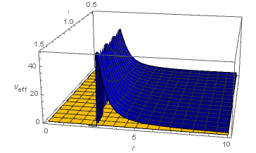
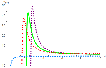
Figure 1: The left-hand plot shows the behavior of the effective potential versus distance and cosmic time while the Right-hand plot shows the effective potential versus distance in some cosmic time. Plots have been depicted with different proper times: $\tau=1.4$ for the dashed-purple plot, $\tau=1$ for the green plot, and $\tau=0.6$ for red-dotted-dashed plot; Blue-Dashed plot has been shown the Schwarzschild case. Furthermore, other numerical considerations are the mass of the black hole, $M=1$, the initial angular momentum of the massless particle, $L=3$, $\rho_{0}=0.0002$, $p_{0}=0.001$, and $t_{BR}=1$.

In the following, we analyze the effective potential in some cosmic epochs with numerical methods. So, as a second step, we fix the black hole’s mass and the particle’s initial angular momentum. About the proper time, we have to notice that we pay attention to some numerical time after forming the black hole horizons while the Big Rip time is equal to 1, $t_{BR}=1$. Therefore, based on our prior research in Ref. 23Es , these numerical times are considered from $t_{1}=-0.4$ until $t_{2}=0.4$. To be precise, two horizons of the LTB black hole have been established before $\tau=1-t_{1}$, and with passing time these two horizons merge and disappear after $\tau=1-t_{2}$. Afterward, we illustrate the effective potential of the cosmological LTB black hole surrounded by a Quintom field in Fig. 1. On the left-hand plot, we show the behavior of an effective potential versus distance and lifetime of the LTB black hole. Also, on the Right-hand plot of Fig. 1, we show the behavior of an effective potential versus distance in some time slices. First of all, we remember that the extremum of an effective potential can indicate the possible location of circular orbits so that the minimum displays the stable orbit while the maximum displays an unstable orbit 03Har . Therefore, based on the illustration of Fig. 1, we conclude that passing time causes: 1. The peak of potential decreases and shifts to fewer radii. 2. The possibility of forming a stable orbit increases.

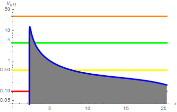
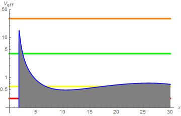
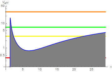
Figure 2: The effective potential of the LTB black hole versus distance in three slices of cosmic epochs. Plots have been depicted left to right by $\tau=1.4,1,0.6$ from early to late time cosmic epochs. Horizontal lines show possible energy for the particle. Other numerical considerations are the mass of the black hole, $M=1$, the initial angular momentum of the massless particle, $L=3$, $\rho_{0}=0.0002$, $p_{0}=0.001$, and $t_{BR}=1$.

For a more detailed explanation, we illustrate the possible energy for the particles in the potential plot in Fig. 2. Plots left to right, demonstrate the passing of time from the early universe to late time epochs. Also, the horizontal lines represent the possible energy for the particles based on Eqs. (2), (3) and, (8). In this figure, we pay attention to there are in general two possible initial positions for the particles: They could come from far away, the horizontal lines on the left side of effective potential- or near the black hole, the horizontal line on the left side of effective potential. Based on the energy and the initial positions of the particle, there are four general situations:

• 1. The red line shows that low-energy particles only can come from near the black hole, are affected by black hole potential, and fall into it. In this situation, the particle follows a Terminating Bound Orbit (See the first row plots in Fig. 3).

• 2. As the particles’ energy increases, it can equal to the minimum of an effective potential. So, the particle falls into the trap of a black hole and goes around it in a Stable circular Orbit. Whereas in the early universe, there is no chance of forming a stable orbit, the possibility has been increased when time passes toward late time epochs. Therefore, if there are more energetic photons, the yellow lines, for the particles which come from far away, two possibilities are expected. In the early universe, particles’ direction changes under the black hole attraction and the particle lies on the kind of a scattering Flyby Orbit (See the left second-row plot in Fig. 3). However, at the late time epochs, the particle moves around the black hole between two turning points and it lies on the Bound Orbit (See middle and right second-row plot in Fig. 3). It is good to mention that the turning points are denoted by crossing the potential curve and yellow line in the middle and right plots in Fig. 2. We emphasize the possibility of this kind of the Bound Orbit is more likely to occur at the late time epochs. Besides, there is another situation for the particle that comes from near the black hole would be, the same item 1, the Terminating Bound Orbit.

• 3. The green line for a particle coming from far away also represents a Flyby Orbit (See third row plots in Fig. 3). To be precise, the flyby orbit describes the situation when a particle comes from far away, its direction changes affected by the black hole’s potential, and finally moves out to infinity again. At this stage, deflection angle could be important for observational research. We will discuss it in the next section. Also like the previous two items, it will be predicted the Terminating Bound Orbit for the particle that comes from near the black hole.

• 4. The energy of a particle can increase again until it exactly reaches the peak of a effective potential so that it goes around the central mass at the unstable orbit. Suppose the particles’ energy is more than the maximum of a effective potential. In the case, an orange line, the particle comes from far away, follows a Terminating Escape Orbit and falls into the black hole.

III.2 Shape of the Orbits

To imagine the shape of orbits, we have to continue with numerical methods. So, first of all, we fix time on the metric and we gain

$$\Big{[}\frac{dr}{d\varphi}\Big{]}^{2}=\frac{e^{2\phi}}{L^{2}}\Bigg{[}\frac{1}{e^{\bar{\phi}}}E^{2}-\frac{e^{\phi}}{e^{\bar{\phi}}}\Big{(}\frac{L}{e^{\phi}}\Big{)}^{2}\Bigg{]}\equiv\chi,$$ (20)

where $E=(\frac{dt}{ds})^{2}$, and $L=e^{\phi}\Big{[}\frac{d\varphi}{ds}\Big{]}^{2}$. We substitute Eqs. (8) and (9) in Eq. (20), and we obtain a differential equation in terms of $r,\varphi,L,$ and $E$ as the following form

$$d\varphi=\frac{dr}{\sqrt{\chi}},$$ (21)

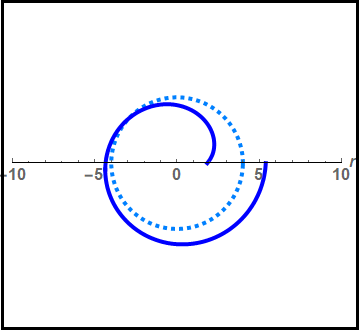
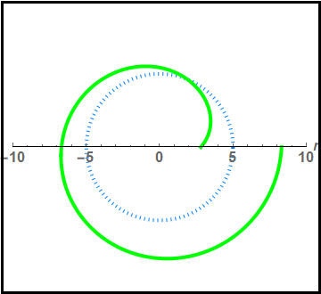
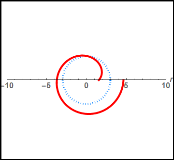
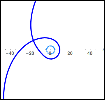
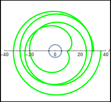
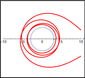
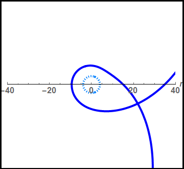
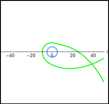
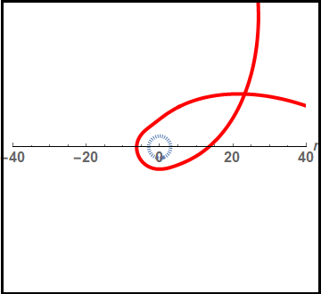
Figure 3: Illustration of the possible orbits around the cosmological black hole in some cosmic epochs. From left to right, time evolves from far away towards near the Big Rip singularity. From top to bottom, the energy of the photon increases. The first row illustrates the terminating bound orbit for a low energy photon moves from near the black hole. If the energy of a photon increases, at the second raw, in the early universe the only possibility is the scattering flyby orbit; While, by moving forward to late time epochs, the possibility of forming the stable bound orbit increases. In this situation, a photon can come from far away and go around the black hole between two turning points. If the energy increases more, a flyby orbit has been expected for all cosmic epochs. Finally, if the photons’ energy is more than the peak of the effective potential, there are figures like the first row except this time a particle comes from far away; It falls into the black hole on the terminating escape orbit. Note that dotted blue circle in the center of each plot shows the cosmological horizon of the black hole.

Next, we put $\tau=1.4,1,0.6$ separately in Eq. (21) and gain three equations. Afterward, substituting $M=1$, $L=3$, $\rho_{0}=0.0002$, $p_{0}=0.001$ we have three numerical differential equations. Finally, Based on Fig. 2, we consider different energy for photons and illustrate the photon’s trajectory in Fig. 3.

If there is a low energy particle in near of the black hole (showed by the red line in Fig. 2), in all cosmic epochs, it falls into the black hole through the terminating bound orbit as we show them in the first row in Fig. 3. Also, this fate are expected for the more energetic particles that we can see at the left side of the effective potential plots as the yellow and green lines. As increasing the energy from red line to yellow line in Fig.2), there is no chance to the formation of stable orbit around the black hole at the early cosmic epochs. Therefore, as expected, we illustrate the scattering flyby orbit at the left second row plot in Fig. 3. As the passing time toward late time epochs, the possibility of a stable orbit formation increases. Therefore, we illustrate a stable orbit for the particle that comes from far away at two remain plots on the second row of Fig. 3. As the energy increases, black hole only can change the trajectory direction and form the flyby orbit for the particle as we illustrate in the third row of Fig. 3. Final possibility is the terminating escape orbit for the particles that have energy more than peak of effective potential at all comic epochs. The trajectory is the same first row of Fig. 3 except the particle comes from far away and get absorbed by the black hole. At all plots in Fig. 3, dotted blue circle shows the largest horizon of the black hole, a cosmological horizon. As mentioned in section 2, we notice that it evolves at size because of the Quintom field existence as the universe content.

III.3 Stability of the Orbits

As we mentioned before, the minimum point of the potential curve indicates the possibility of forming a circular orbit around the black hole. Our investigations in the previous section illustrated that after the formation of this circular orbit in the near past, the radius increases as the black hole moves in the accelerated universe towards the Big Rip singularity. This section aims to investigate some aspects of the stable orbits in a certain cosmic epoch near the Big Rip singularity. Therefore, we fix time to $\tau=0.6$ and find out with the numerical analysis of Eq. III.1, there is the specified range for $1\leq L<4$ in which the behavior of potential is preserved. Moreover, as we illustrate in Fig. 4 the radius of an Innermost Stable Circular Orbit (ISCO) increases while $L$ increases. In other words, whenever $L$ becomes greater, two extremum of the potential shift to the larger radii. Furthermore, by increasing $L$, more energetic photons can be attracted by a black hole in the circle or general bound orbit. Besides, approaching two extremes to each other, the possibility of the bound orbit formation decreases, and the probability of deviation in the photon direction as a flyby orbit increases.

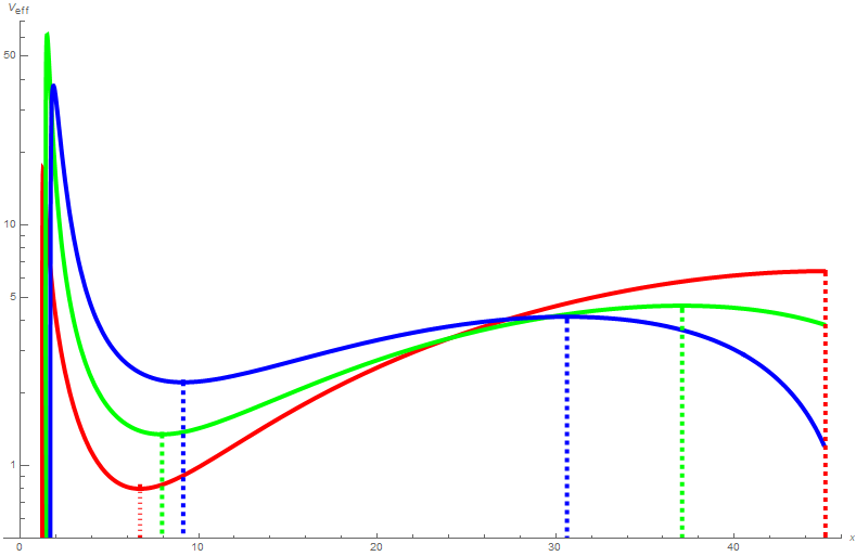
Figure 4: The behavior of the Effective Potential versus distance. Plots have been depicted with $L=1,1.8,3$ left to right and, fixed mass $M=1$, while $\rho_{0}=0.0002$, $p_{0}=0.001$, and $\tau=0.6$.

III.4 Outlook

In this research, we have demonstrated evidence of the orbit evolution around a black hole in the accelerated universe from the early toward late time epochs. As a forward step, based on our previous in-depth research in Refs. 16Sor , we are interested in numerically investigating the Kerr-Newman black hole in the accelerated universe. In particular, studies about the orbit stability and deflection angle could be important for observing early galaxies and x-ray resources.

IV Discussion and Conclusion

In this paper, we have considered the LTB black hole as a kind of cosmological black hole in the accelerated universe filled by the Quintom field. Indeed, as well the Quintom field provided a fine description for crossing -1 of the equation of state, the LTB black hole describes the black hole in the accelerated universe. After an introduction to the metric of such a black hole, we have gained the explicit equation for the effective potential of the massless particle around the LTB black hole surrounded by the Quintom field. As we emphasized, the characterized feature of the cosmological black hole is time evolution. Therefore, we have probed in the time evolution of an effective potential for the LTB black hole in the accelerated universe with Quintom content. Moreover, we conclude that whenever we consider passing time from the early universe until the late time cosmic epochs, the peak of the black hole’s potential decreases and shifts to the smaller radii. Also, when we get closer to the late time epochs, the possibility of forming a minimum in the potential and therefore founding of the stable orbit for the particle increases. In the following, we have investigated the type of the particles’ orbit based on their energy and distance from the LTB black hole in some slices of cosmic epochs. We have concluded that in the different cosmic epochs, we face variant situations for black hole geodesics, which indicates that the particles’ orbits, and subsequently predicting observational effects like light deflection, and perihelion shift can also be different. In all cosmic epochs, four situations can exist: 1. The near-located particle of an LTB black hole can follow the Terminating Bound Orbit and fall into the black hole. 2. Moving forward from the early universe towards late time epochs, there is a specific range of particles’ energy and distance from the black hole in which the Stable or Bound Orbit have been formed. To be precise, the possibility of forming a circular orbit around the LTB black hole in the accelerated universe increases as time evolves toward late time epochs. 3. A highly energetic particle far from the LTB black hole can be affected by the gravitational field, change its direction by following the Flyby Orbit, then escape to infinity. 4. A far from particle with higher energy from the potential’s peak could follow the Terminating escape orbit, and fall into the black hole. In the final step, we have also examined the role of angular momentum on the orbital stability in a certain cosmic time slice, and have shown that increasing it causes approach two extremes of the effective potential and decreasing the possibility of a Bound Orbit formation.

Acknowledgment

We would like to appreciate Kourosh Nozari for helpful discussion and insightful comments on the original draft of this manuscript.

References

- (1) G. C. McVittie, “The Mass-Particle in an Expanding Universe”, Mon. Not. R. Astron. Soc. 93, 325 (1933), [10.1093/mnras/93.5.325].
- (2) A. Einstein, E. G. Straus, “The Influence of the Expansion of Space on the Gravitation Fields Surrounding the Individual Stars”, Rev. Mod. Phys. 17, 120 (1945), [10.1103/RevModPhys.17.120].
- (3) P. C. Vaidya, “The Kerr metric in cosmological background”, Pramana 8, 512 (1977), [10.1007/BF02872099].
- (4) R. C. Tolman, “Effect of Inhomogeneity on Cosmological Models”, Proc. Nat. Acad. Sci. 20, 169 (1934), [10.1073/pnas.20.3.169].
- (5) H. Bondi, “Spherically Symmetrical Models in General Relativity”, M. Not. of the R. A. Soc. 107, 410 (1947), [10.1093/mnras/107.5-6.410].
- (6) G. Lemaître, “The expanding universe”, Gen. Rel. Grav. 29, 641 (1997), [10.1023/A:1018855621348].
- (7) S. A. Hayward, “General Laws of Black-Hole Dynamics”, Phys. Rev. D 49, 6467 (1994), [10.1103/PhysRevD.49.6467].
- (8) A. Ashtekar, B. Krishnan, “Dynamical Horizons: Energy, Angular Momentum, Fluxes and Balance Laws”, Phys. Rev. Lett. 89, 261101 (2002), [10.1103/PhysRevLett.89.261101].
- (9) V. Faraoni, V. Vitagliano, “Horizon thermodynamics and spacetime mappings”, Phys. Rev. D 89, 064015 (2014), [10.1103/PhysRevD.89.064015].
- (10) V. Faraoni, “Cosmological and Black Hole Apparent Horizons”, Lect.Notes Phys. 907, 1 (2015), [10.1007/978-3-319-19240-6].
- (11) J. T. Firouzjaee, R. Mansouri,, “Asymptotically FRW black holes”, Gen. Rel. Grav. 42, 2431 (2010), [10.1007/s10714-010-0991-7].
- (12) Ch. Gao, X. Chen, Y. G. Shen, V. Faraoni, “Black Holes in the Universe: Generalized Lemaître-Tolman-Bondi Solutions”, Phys. Rev. D 84, 104047 (2011), [10.1103/PhysRevD.84.104047].
- (13) N. Chakraborty, B. Subenoy, and R. Mazumder, “Thermodynamics of Lemaître-Tolman-Bondi Model”, Gen. Rel. Grav. 43, 1827 (2011), [10.1007/s10714-011-1160-3].
- (14) S. M. Koksbang, A. Heinesen,“Redshift drift in a universe with structure: Lemaître-Tolman-Bondi structures with arbitrary angle of entry of light,” Phys. Rev. D 106 043501 (2022), [10.1103/PhysRevD.106.043501].
- (15) T. Schiavone, G. Montani,“Signature of f(R) gravity via Lemaître-Tolman-Bondi inhomogeneous perturbations,” Eur. Phys. J. C 84, 490 (2024), [10.1140/epjc/s10052-024-12842-2].
- (16) Sh. Tsujikawa, “Quintessence: A Review”, Class. Quant. Grav. 30, 214003 (2013) , [10.1088/0264-9381/30/21/214003].
- (17) R. R. Caldwell, “A Phantom Menace? Cosmological consequences of a dark energy component with super-negative equation of state”, Phys. Lett. B 545, 23 (2002) , [10.1016/S0370-2693(02)02589-3].
- (18) C. Armendariz-Picon, V. Mukhanov, P. J. Steinhardt, “Essentials of k-essence”, Phys. Rev. D 63, 103510 (2001) , [10.1103/PhysRevD.63.103510].
- (19) A. Sen, “Tachyon Matter”, JHEP 0207, 065 (2002) , [10.1088/1126-6708/2002/07/065].
- (20) E. Elizalde, S. Nojiri, S. D. Odintsov, “Late-time cosmology in (phantom) scalar-tensor theory: Dark energy and the cosmic speed-up,” Phys. Rev. D 70, 043539 (2004), [10.1103/PhysRevD.70.043539].
- (21) B. Feng, X. L. Wang, X. M. Zhang , “Dark energy constraints from the cosmic age and supernova”, Phys. Lett. B 607, 35 (2005), [10.1016/j.physletb.2004.12.071].
- (22) K. Nozari, M. R. Setare, T. Azizi and N. Behrouz, “A Non-minimally Coupled Quintom Dark Energy Model on the Warped DGP Brane”, Phys. Scripta 80, 025901 (2009), [10.1088/0031-8949/80/02/025901].
- (23) Y. F. Cai, E. N. Saridakis, M. R. Setare, J. Q. Xia , “Quintom Cosmology: Theoretical implications and observations”, Phys. Rept. 493, 1 (2010), [10.1016/j.physrep.2010.04.001].
- (24) K. Nozari and N. Behrouz, “An Interacting Dark Energy Model with Nonminimal Derivative Coupling”, Phys. Dark Univ. 13, 92-110 (2016), [10.1016/j.dark.2016.04.004].
- (25) E. Elizalde, S. Nojiri, S. D. Odintsov, D. Saez-Gomez and V. Faraoni,“Reconstructing the universe history, from inflation to acceleration, with phantom and canonical scalar fields,” Phys. Rev. D 77, 106005 (2008), [10.1103/PhysRevD.77.106005].
- (26) C. Gao, X. Chen, V. Faraoni and Y. G. Shen,“Does the mass of a black hole decrease due to the accretion of phantom energy,”, Phys. Rev. D 78, 024008 (2008), [10.1103/PhysRevD.78.024008].
- (27) A. Leithes,“Perturbations in Lemaitre-Tolman-Bondi and Assisted Coupled Quintessence Cosmologies”, [1704.08975 [astro-ph.CO]].
- (28) D. Farrah, K. S. Croker, G. Tarlé, V. Faraoni, S. Petty, J. Afonso, N. Fernandez, K. A. Nishimura, C. Pearson and L. Wang, et al. “Observational Evidence for Cosmological Coupling of Black Holes and its Implications for an Astrophysical Source of Dark Energy”, Astrophys. J. Lett. 944 L31 (2023), [10.3847/2041-8213/acb704].
- (29) S. Soroushfar, R. Saffari, J. Kunz and C. Lämmerzahl,“Analytical solutions of the geodesic equation in the spacetime of a black hole in f(R) gravity”, Phys. Rev. D 92, 044010 (2015), [10.1103/PhysRevD.92.044010].
- (30) S. Soroushfar, R. Saffari, S. Kazempour, S. Grunau and J. Kunz, “Detailed study of geodesics in the Kerr-Newman-(A)dS spacetime and the rotating charged black hole spacetime in gravity”, Phys. Rev. D 94, 024052 (2016), [10.1103/PhysRevD.94.024052].
- (31) S. Soroushfar and M. Afrooz,“Analytical solutions of the geodesic equation in the space-time of a black hole surrounded by perfect fluid in Rastall theory”, Indian J. Phys. 96, 593 (2022), [10.1007/s12648-020-01971-5].
- (32) B. C. Nolan,“Particle and photon orbits in McVittie spacetimes”, Class. Quant. Grav. 31, 235008 (2014), [10.1088/0264-9381/31/23/235008].
- (33) I. Antoniou, L. Perivolaropoulos,“Geodesics of McVittie Spacetime with a Phantom Cosmological Background”, Phys. Rev. D 93, 123520 (2016), [10.1103/PhysRevD.93.123520].
- (34) G. A. Baker, Jr.,“Effects on the structure of the universe of an accelerating expansion”, Gen. Rel. and Grav. 34 767 (2002), [10.1023/A:1016371629024].
- (35) S. Nesseris and L. Perivolaropoulos,“The Fate of bound systems in phantom and quintessence cosmologies”, Phys. Rev. D 70, 123529 (2004), [10.1103/PhysRevD.70.123529].
- (36) M. -N. Celerier, “Do we really see a cosmological constant in the supernovae data?”, Astron. Astrophys. 353, 63 (2000), [10.48550/arXiv.astro-ph/9907206].
- (37) S. Eslamzadeh, K. Nozari, J. T. Firouzjaee, “Cosmological LTB Black Hole in a Quintom Universe”, Eur. Phys. J. C 83, 1057 (2023), [10.1140/epjc/s10052-023-12215-1].
- (38) P. J. E. Peebles, “Principles of Physical Cosmology”, Princeton University Press, Princeton NJ (1993), [ 9780691209814].
- (39) J. B. Hartle,“Gravity: An introduction to Einstein’s general relativity”, Addison-Wesley Pub. Co., Boston (2003), [9780805386622].