Constrained Learning for Decentralized Multi-Objective Coverage Control

Abstract

The multi-objective coverage control problem requires a robot swarm to collaboratively provide sensor coverage to multiple heterogeneous importance density fields (IDFs) simultaneously. We pose this as an optimization problem with constraints and study two different formulations: (1) Fair coverage, where we minimize the maximum coverage cost for any field, promoting equitable resource distribution among all fields; and (2) Constrained coverage, where each field must be covered below a certain cost threshold, ensuring that critical areas receive adequate coverage according to predefined importance levels. We study the decentralized setting where robots have limited communication and local sensing capabilities, making the system more realistic, scalable, and robust. Given the complexity, we propose a novel decentralized constrained learning approach that combines primal-dual optimization with a Learnable Perception-Action-Communication (LPAC) neural network architecture. We show that the Lagrangian of the dual problem can be reformulated as a linear combination of the IDFs, enabling the LPAC policy to serve as a primal solver. We empirically demonstrate that the proposed method (i) significantly outperforms existing state-of-the-art decentralized controllers by 30% on average in terms of coverage cost, (ii) transfers well to larger environments with more robots and (iii) is scalable in the number of fields and robots in the swarm.

I Introduction

In a multi-objective coverage control problem, an environment is characterized by importance density fields representing the relative significance of different regions, each capturing a distinct environmental aspect from various information sources. Depending on the requirements, one may use a fair coverage strategy for equitable resource distribution across all fields or a constrained coverage strategy to satisfy specific constraints associated with individual fields.

Fair coverage minimizes the maximum coverage cost for any field, promoting equal resource allocation. For instance, in a flooding scenario, a swarm of robots is deployed to provide sensor coverage over a large urban area. While the central city region is critical, the outskirts also need monitoring. A single importance field might cause robots to cluster in the city, neglecting other areas. A fair coverage strategy ensures robots are distributed across the entire region, providing adequate coverage to all areas, which is crucial in humanitarian applications where resources must be fairly allocated [1].

Constrained coverage requires each field to be covered below a certain cost threshold, ensuring critical areas receive coverage according to predefined importance levels. In wildfire monitoring, defining a single field for all relevant information is challenging. Instead, multiple importance fields—such as vegetation density, proximity to habitation, and historical data—provide a comprehensive environmental view. Setting a cost threshold for each field ensures minimum information acquisition for each aspect, guaranteeing critical areas are appropriately monitored.

To address these optimization problems, we develop a novel decentralized constrained learning approach that combines primal-dual optimization with a Learnable Perception-Action Communication (LPAC) neural network architecture [2]. Specifically, we employ a primal-dual algorithm utilizing the Lagrangian dual, which periodically updates the dual variables, and the LPAC policy serves as the primal solver. The LPAC architecture uses convolutional neural networks (CNNs) to extract features from the robots’ local perceptions, graph neural networks (GNNs) to model inter-robot communication, and a shallow multilayer perceptron (MLP) to output robot actions in terms of velocities. The GNN is the primary collaborative component in LPAC as it decides what information to communicate and how to use received information with its own perception. This design enables robots to make informed decisions based on local information and limited communication, ensuring scalability and efficiency in decentralized settings.

Contributions:

1. We present a novel method that combines primal-dual optimization with the LPAC architecture to solve decentralized multi-objective coverage problems for fair and constrained coverage with limited communication and sensing capabilities of robots.

2. The Lagrangian of the dual problem is reformulated as a linear combination of fields, allowing the multi-objective coverage control problem to be recast as a dynamically re-weighted single-objective problem.

3. Extensive empirical studies demonstrate the effectiveness of the proposed method compared to existing centroidal Voronoi tessellation methods. Our approach achieves an average improvement of $30\%$ in coverage cost, with peak improvements of up to 100%.

4. We establish the scalability and transferability of the proposed method in terms of (a) the number of robots, (b) the size of the environment, and (c) the number of importance fields.

I-A Related Work

Coverage Control is widely studied in robotics with applications in mobile networking [3], surveillance [4], and target tracking [5]. The foundations of decentralized control algorithms for robots with limited sensing and communication capabilities were given by Cortés et al. [6]. The algorithms iteratively perform (i) a centroidal Voronoi tessellation (CVT) [7, 8] of the environment and assigns each robot to their respective Voronoi cell, and (ii) computes the centroid of each cell and moves the robot towards it. The algorithms are also referred to as variants of the Lloyd’s algorithm [9] from quantization theory. However, there has been a limited study on coverage control with multiple importance fields.

Socially fair coverage control in the context of multiple importance density fields arising from population groups was studied by Malencia et al. [1]. They use a relaxation of the min-max problem by using LogSumExp approximation, and design a control law based on this relaxation.

Our approach tackles multi-objective coverage problems in a principled way through duality, recasting them as a single objective coverage control and therefore allowing any coverage control policy to generalize to the multi-objective case without the need for retraining or redesigning controllers.

Graph Neural Networks are cascaded architectures composed of layers of graph convolutions and pointwise non-linearities [10]. GNNs have shown impressive results in problems like weather prediction [11], recommendation systems [12], and physics [13]. Given their graph convolutional structure, GNNs can be used for decentralized problems and have been proven useful in various robotics applications such as multi-robot active information acquisition [14], coverage control [15, 2], and path planning [16, 17, 18]. Given their theoretical properties, GNNs are well-suited for robotic applications; GNNs are stable to perturbations on the graph [19, 20], are transferable to larger scale graphs [21], and generalize to unseen graphs [22].

Constrained learning is a machine learning technique that tackles problems in which more than one objective needs to be satisfied jointly [23, 24]. Notable applications of constrained learning range from federated learning [25], passing through robustness [26] and smoothness [27], to active learning [28]. Constrained learning has found applications in GNNs for improving their stability [29], and robustness [30]. In terms of robotics, constrained learning has found applications in safe reinforcement learning [31, 32, 33] and legged robot locomotion [34].

II Decentralized Multi-Objective Coverage

We consider a $d$-dimensional environment ${\mathcal{W}}\subset{\mathbb{R}}^{2}$, and a homogeneous set of $N$ robots ${\mathcal{V}}=\{1,\dots,N\}$. The position of the robot at time $t$ is denoted by $\mathbf{p}_{i}(t)\in{\mathcal{W}}$. Robots take control actions $\mathbf{u}_{i}(t)\in{\mathbb{R}}^{2}$ to move in the environment and follow a single integrator dynamics, i.e.,

$$\mathbf{p}_{i}(t+\Delta t)=\mathbf{p}_{i}(t)+\Delta t\mathbf{u}_{i}(t),$$ (1)

where $\Delta t$ is the time step.

In a decentralized setting, each agent makes observations of its local environment and communicates with nearby robots to exchange information. We define a communication graph graph ${\mathcal{G}}=({\mathcal{V}},{\mathcal{E}})$, where ${\mathcal{V}}$ is the set of robots, and ${\mathcal{E}}$ is the set of edges that represents a communication link between the robots. The communication link $(i,j)\in{\mathcal{E}}$ exists if the distance between the robots $i$ and $j$ is less than the communication radius $r_{c}$, i.e. $\|\mathbf{p}_{i}-\mathbf{p}_{j}\|\leq r_{c}$. We assume the communication to flow both ways and, therefore, the graph to be undirected. A robot may communicate an abstract representation of its state with its neighbors, and the communication graph is used to determine the neighborhood of each robot. Decentralized policies are executed by each robot independently, and do not require a centralized server thus alleviating the communication and scalability issues.

In coverage control, the objective is to provide sensor coverage based on the relative importance of each point in the environment. We define an importance density field (IDF) $\Phi:{\mathcal{W}}\to{\mathbb{R}}^{+}$, which represents the importance of each point in the environment. The cost function ${\mathcal{J}}$ is thus defined as,

$${\mathcal{J}}({\mathbf{X}}(t))=\int_{{\mathbf{q}}\in{\mathcal{W}}}\min_{i\in{\mathcal{V}}}f(||{\mathbf{p}}_{i}-{\mathbf{q}}||)\Phi({\mathbf{q}})d({\mathbf{q}}),$$ (2)

where $f$ is a non-decreasing function, and a common choice is $f(x)=x^{2}$. The state of the system is given by ${\mathbf{X}}(t)=\{{\mathbf{p}}_{i}(t)\}_{i\in{\mathcal{V}}}$. Assuming that two robots cannot occupy the same point, we can assign each robot a distinct portion of the environment to cover based on the Voronoi partitions [35], and the cost function can be rewritten as,

$$\mathcal{J}\left(\mathbf{X}(t)\right)=\sum_{i=1}^{N}\int_{\mathbf{q}\in P_{i}}f(\|\mathbf{p}_{i}(t)-\mathbf{q}\|)\Phi(\mathbf{q})\,d\mathbf{q},$$ (3)

where $P_{i}$ is the Voronoi partition of robot $i$.

II-A Multi-Objective Coverage

In multi-objective coverage, we are given $M$ IDFs $\Phi_{m}:{\mathcal{W}}\to{\mathbb{R}}^{+}$, and we formulate two problems. The first problem, fair coverage, aims to minimize the maximum coverage cost of any IDF. The second problem, constrained coverage, aims to minimize the cost function of one IDF while ensuring that the cost functions of the other IDFs are below a certain threshold.

Fair Coverage: Given a team of $N$ robots operating in an environment with $M$ IDFs, the Fair Multi-Objective Coverage Problem (FMCP) is defined as,

$$P_{f}=\min_{{\mathbf{X}}(t),\rho}\quad \rho$$ (FMCP)

subject to $${\mathcal{J}}_{m}({\mathbf{X}}(t))\leq\rho\quad\forall\,m=1,\dots,M$$

In the FMCP, all coverage functions need to be below $\rho$. This is typically called an epigraph problem [36].

Constrained Coverage: Given a team of $N$ robots operating in an environment with $M$ IDFs, the Constrained Multi-Robot Coverage Problem (CMCP) is defined as,

$$P_{c}=\min_{{\mathbf{X}}(t)}\quad {\mathcal{J}}_{0}({\mathbf{X}}(t))$$ (CMCP)

subject to $${\mathcal{J}}_{m}({\mathbf{X}}(t))\leq\alpha_{m}\quad\forall\,m=1,\dots,M$$

Note that in the CMCP, there are $M+1$ objectives that need to be covered. The $0$-th one needs to be minimized while the other $M$ of them need to be covered up to their corresponding $\alpha_{m}$. Note that the $0$-th objective is not necessary, and the formulation can be used to obtain feasible solutions that satisfy the constraints.

III Primal-Dual Algorithm for Multi-Objective Coverage

To solve the multi-objective coverage control problem, we resort to the dual domain. To this end, we introduce the dual variables $\lambda_{i}\geq 0,i\in[0,M],\boldsymbol{\lambda}=[\lambda_{1},\dots,\lambda_{M}]$, and define the constrained ${\mathcal{L}}_{c}$ and fair ${\mathcal{L}}_{f}$ Lagrangians as,

$${\mathcal{L}}_{f}({\mathbf{X}}(t),\boldsymbol{\lambda}) :=\sum_{m=1}^{M}\lambda_{m}{\mathcal{J}}_{m}({\mathbf{X}}(t)),\text{s.t.}\sum_{i=1}^{M}\lambda_{i}=1,$$ (4)

$${\mathcal{L}}_{c}({\mathbf{X}}(t),\boldsymbol{\lambda}) :=\sum_{t=0}^{T}{\mathcal{J}}_{0}({\mathbf{X}}(t))+\sum_{m=1}^{M}\lambda_{m}({\mathcal{J}}_{m}({\mathbf{X}}(t))-\alpha_{m})$$ (5)

Note that the variable $\rho$ disappears from the Lagrangian ${\mathcal{L}}_{f}$, as it is a property of the solution (see [27, Appendix A ]).

To obtain the optimal values of the dual variables $\boldsymbol{\lambda}$, we return to the Lagrangian ${\mathcal{L}}_{*},*\in\{f,c\}$, we can express the dual function as

$$d_{*}(\boldsymbol{\lambda}):=\min_{{\mathbf{X}}(t)}{\mathcal{L}}_{*}({\mathbf{X}}(t),\boldsymbol{\lambda}).$$ (6)

Note that the dual function is a concave function of $\boldsymbol{\lambda}$ [36], and we can therefore take the maximum thus defining the dual problem as,

$$D_{*}=\max_{\boldsymbol{\lambda}}d_{*}(\boldsymbol{\lambda}).$$ (7)

Through duality, we can solve the primal problem $P_{f}$ (FMCP) or $P_{c}$ (CMCP) by its dual counterpart $D_{*}$ (cf. (7)). This is useful because while the primal problem is a constrained optimization problem for whom even finding a feasible solution is non-trivial, the dual problem $D_{*}$ is a linear combination of optimization problems that can be solved in practice. To solve dual problem (7), we need to realize the fact that it is equivalent to a single IDF coverage control problem.

Proposition 1.

Given a set of scalars $\lambda_{m}\geq 0,m=1,\dots,M$, the linear combination of coverage control problems $\sum_{m=1}^{M}\lambda_{i}{\mathcal{J}}_{\phi_{m}}({\mathbf{X}}(t))$, is equivalent to a coverage control problem on the linear combinations of IDFs, i.e. ${\mathcal{J}}_{\phi_{\lambda}}({\mathbf{X}}(t))$, with $\phi_{\lambda}(x)=\sum_{m=1}^{M}\lambda_{i}\phi_{m}(x).$

Proof.

We can start with the definition of ${\mathcal{J}}$, and by linearity of integration,

$$\sum_{m=1}^{M}\lambda_{m}{\mathcal{J}}_{m}({\mathbf{X}}(t)) =\sum_{m=1}^{M}\lambda_{m}\int_{{\mathbf{q}}\in{\mathcal{W}}}f(||{\mathbf{p}}_{i}(t)-{\mathbf{q}}||)\phi_{m}({\mathbf{q}})d{\mathbf{q}}$$

$$=\int_{{\mathbf{q}}\in{\mathcal{W}}}f(||{\mathbf{p}}_{i}(t)-{\mathbf{q}}||)\sum_{m=1}^{M}\lambda_{m}\phi_{m}({\mathbf{q}})d{\mathbf{q}}.$$

Note that $\sum_{m=1}^{M}\lambda_{m}\phi_{m}(x)$ is a valid IDF as $\lambda\geq 0$. By defining $\phi_{\lambda}(x)=\sum_{m=1}^{M}\lambda_{m}\phi_{m}(x)$, we obtain the result. ∎

Proposition 1 states that a linear combination of coverage control problems is equivalent to a coverage control problem on the linear combinations of IDFs. Although simple, this result opens the door to solving the multi-objective coverage control as a single coverage control problem on the linear combination of IDFs.

Corollary 2.

The dual function (6) associated with Lagrangian ${\mathcal{L}}_{f}({\mathbf{X}}(t),\boldsymbol{\lambda})$ of the fair coverage control problem and Lagrangian ${\mathcal{L}}_{c}({\mathbf{X}}(t),\boldsymbol{\lambda})$ are equivalent to a single objective unconstrained coverage control problem with $\phi_{\boldsymbol{\lambda}}({\mathbf{q}})=\sum_{m=1}^{M}\lambda_{m}\phi_{m}({\mathbf{q}})$.

Proof.

We can apply Proposition 1 to the Lagrangians ${\mathcal{L}}_{f}$ and ${\mathcal{L}}_{c}$. By defining $\phi_{\boldsymbol{\lambda}}({\mathbf{q}})=\sum_{m=1}^{M}\lambda_{m}\phi_{m}({\mathbf{q}})$, and noting that this is a valid IDF given that $\lambda\geq 0$, we complete the proof. It should be noted that for the constrained Lagrangian ${\mathcal{L}}_{c}$, the term $\sum_{m=1}^{M}\lambda_{m}\alpha_{m}$ is a constant and does not take part in the minimization. ∎

Corollary 2 is important because it allows us to simplify the multi-objective coverage control problem by recasting it as a single objective, thus utilizing a policy $\pi$ for a single coverage control. The case with constraints ${\mathcal{L}}_{c}$, is equivalent for the minimization problem. Under mild assumptions, and both for convex as well as non-convex losses, it can be shown that the constrained optimization problem $P_{*}$, and the dual counterpart $D_{*}$ are close [24, 23, 37].

III-A Primal-Dual Algorithm For Multi-Objective Coverage

To obtain the optimal dual variables and solve the dual problem 7, we will resort to a primal-dual algorithm. There are two time frames, the primal and the dual time frame, the dual being slower than the primal, i.e., the value of $\lambda$ remains constant over a $T$ period, upon which it is modified.

In the primal update, at time step $k$, given dual variables $\boldsymbol{\lambda}_{k}$, the objective is to find the action such that the objective ${\mathcal{J}}_{\boldsymbol{\lambda}_{k}}({\mathbf{X}}(t))$ is minimized. After $T$ steps, the dual variables get updates according to the following rules:

$$\tilde{\lambda}_{k+1}^{i}=[\lambda_{k}^{i}+\eta s(k)^{i}]_{+}\text{ (dual update),}$$ (8)

$$\boldsymbol{\lambda}_{k+1}^{i}={\mathcal{P}}[\tilde{\lambda}_{k+1}^{i}]\text{ (dual projection),}$$ (9)

where $s^{i}$ represents the slackness (or constraint satisfaction) of the $i$-th constraint, and ${\mathcal{P}}$ is a projection. In the case of constrained multi-objective coverage (CMCP), takes the form

$$s^{i}_{c}(k)=\frac{1}{T}\sum_{t=kT}^{(k+1)T}({\mathcal{J}}_{i}\left({\mathbf{X}}(t)\right)-\alpha_{i},$$ (10)

and there is no projection, i.e. $\tilde{\boldsymbol{\lambda}}=\boldsymbol{\lambda}$. In the case of fair coverage (FMCP), the dual update takes the form,

$$s^{i}_{f}(k)=\frac{1}{T}\sum_{t=kT}^{(k+1)T}{\mathcal{J}}_{i}\left({\mathbf{X}}(t)\right)$$ (11)

and the projection is

$$\boldsymbol{\lambda}= \operatorname*{arg\,min}_{\boldsymbol{\lambda}}||\boldsymbol{\lambda}-\tilde{\boldsymbol{\lambda}}||_{2}\text{ s.t. }\sum_{m=1}^{M}\lambda_{m}=1.$$ (12)

This projection is required to satisfy the constraint added to the Lagrangian, (cf. equation (4)). A succinct explanation of the primal-dual steps can be found in Algorithm 1.

  Input: Policy $\pi$, initial dual variables $\boldsymbol{\lambda}$, dual period $T$, dual stepsize $\eta$, total number of dual steps $K$

  for $k=1$ to $K$ do

     for $t=1$ to $T$ do

        Obtain action for current state ${\mathbf{U}}(t)\leftarrow\pi({\mathbf{X}}(t),\phi_{\boldsymbol{\lambda}})$.

        Perform control actions ${\mathbf{U}}(t)$.

     end for

     Update dual variables according to (8).

     Project dual variables according to (9).

  end for

Algorithm 1 Primal Dual Algorithm For Multi-Objective Coverage

IV Perception Action Communication Loops

Intelligent collaborative and decentralized robotic systems require each robot to independently perceive the environment, communicate information with nearby neighbors, and take appropriate actions by using all the received and sensed information. This leads to a Perception-Action-Communication (PAC) loop. In a Learnable PAC (LPAC) architecture [2], we have a neural network for each of the three modules: a Convolutional Neural Network (CNN) for perception, a Graph Neural Network (GNN) for communication, and a Multi-Layer Perceptron (MLP) for action. We train the LPAC architecture using imitation learning, where we use a centralized clairvoyant CVT-based controller is used to generate target actions for the robots.

Environment setup: Robots are initialized uniformly at random in a square environment with side length $1024\,\text{m}$ and a resolution of $1\,\text{m}$ per pixel. For each importance density field (IDF), we generate a fixed number of 2D Gaussian distributions, where the mean is uniformly sampled in the environment, and the variance is sampled from $[40,60]$ with a limit of $3$ standard deviations to avoid detection from afar. Each such distribution is scaled by a random factor sampled from $[0.05,1.00]$ to have a wide range of importance values.

As robots move, they maintain an importance map for each IDF to store observations and a boundary map to store perceived boundaries. The observations are limited to a $64\times 64$ window around the robot. The robots follow a single integrator dynamics with a maximum speed of $1\,\text{m}\cdot{}\text{s}^{-1}$.

We now describe the three modules of the architecture.

The perception module comprises a CNN that takes as input a four-channel image representing the importance field, the boundary, and the $x$ and $y$ coordinates of the nearby robots. A local region of $256\times 256$ pixels is extracted from the importance maps and the boundary map, and they are scaled down to $32\times 32$ pixels; this forms the first two channels of the input. The $x$ and $y$ relative coordinates of the neighboring robots are scaled by the communication range and are added as the third and fourth channels, respectively.

The CNN consists of three sequences, each comprising a convolutional layer followed by batch normalization [38] and a leaky ReLU activation function. Each convolutional layer uses a $3\times 3$ kernel with a stride of one and zero padding, producing 32 output channels. The output of the final sequence is flattened and passed through a linear layer with a leaky ReLU activation to generate a 32-dimensional feature vector. This feature vector is then sent to the communication module for further processing.

The communication module receives the feature vector from the perception module and propagates it through the communication graph using a Graph Neural Network (GNN). The GNN computes a message for each robot that needs to be communicated to other agents. Furthermore, the GNN aggregates the received messages and combines them with the local feature vector to generate the final output, which is passed to the action module.

Our GNN architecture is a composition of $5$ graph convolution filters [39] with ReLU as the pointwise nonlinearity. Each convolution is parameterized by $k=3$ hops, and each layer has $512$ hidden units. The shift operator $S$ is the normalized adjacency matrix of the communication graph,

$$\mathbf{S}=\mathbf{D}^{-1/2}\mathbf{A}\mathbf{D}^{-1/2},$$ (13)

$\mathbf{A}$ is the adjacency matrix, and $\mathbf{D}$ is the diagonal degree matrix. Each layer is given by:

$$\mathbf{Z}_{l}=\sum_{k=0}^{K}(\mathbf{S})^{k}\mathbf{X}_{l-1}\mathbf{H}_{lk},\quad\mathbf{X}_{l}=\sigma(\mathbf{Z}_{l}).$$ (14)

Here $\mathbf{X}_{l}$ is the output of the $l$-th layer, $\mathbf{H}_{lk}$ is the weight matrix of the $k$-th filter in the $l$-th layer, and $\sigma$ is the ReLU activation function.

The action module is the last link of the chain and is in charge of generating the local velocity control action for the robot. The MLP has two layers with 32 units each, and the final output of the MLP is processed by a linear layer to generate the $x$ and $y$ components of the velocity action.

IV-A Imitation Learning

We use imitation learning to train the LPAC architecture to mimic the behavior of the clairvoyant algorithm. The training is performed using the Adam optimizer [40] in Python using PyTorch [41] and PyTorch Geometric [42]. We use a batch size of 100 and train the network for 100 epochs, with a learning rate of $10^{-4}$ and a weight decay of $10^{-3}$. We use the mean squared error (MSE) loss as the loss function, where the target is the output of the clairvoyant algorithm, and the prediction is the output of the LPAC architecture. The model with the lowest validation loss is selected as the final model.

V Experiments

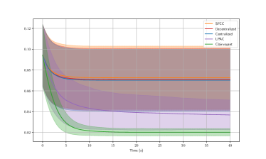
Figure 1: Fair multi-objective coverage control problem with $32$ robots and $4$ IDFs in a $1024\times 1024$ $\,\text{m}^{2}$ environment. The coverage cost increase in comparison to the clairvoyant is $81\%$, $246\%$, $250\%$, and $258\%$ for LPAC, Centralized, Decentralized, and SFCC [1] respectively.

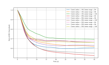
Figure 2: Fair coverage control with the LPAC controller normalized by the CVT controller for various communication radius and sensor sizes.

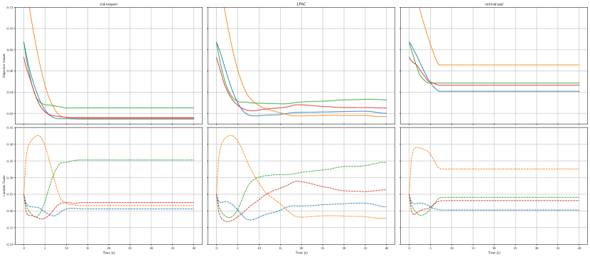
Figure 3: Case study: Correlation of maximum coverage cost (top row) and dual variables (bottom row) per IDF for a specific environment. Each color represents a different IDF. The columns are clairvoyant, LPAC, and centralized controllers in order.

TABLE I: Fair Coverage: Varying Number of Robots

# Robots	# Best Environments		Average Max Objective
	Centralized CVT	LPAC	Centralized CVT	LPAC
8	32	68	2.839	2.763
16	15	85	2.680	2.191
24	4	96	2.559	1.687
32	6	94	2.251	1.386
40	2	98	2.167	1.191
48	6	94	1.842	1.163
56	3	97	1.744	0.981
64	3	97	1.608	0.983

TABLE II: Fair Coverage: Varying Number of IDFs

# IDFs	# Best Environments		Average Max Objective
	Centralized CVT	LPAC	Centralized CVT	LPAC
4	6	94	2.251	1.386
5	6	94	3.137	1.979
6	5	95	4.144	2.486
7	4	96	5.072	3.214
8	4	96	6.144	3.792
9	1	99	7.060	4.667
10	0	100	8.104	5.037

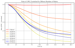
(a) Robot ablation. The performance ratio between LPAC and Centralized as a function of time for the fair coverage control problem. We vary the number of robots by steps of $8$, from $8$ to $64$ with $1024\times 1024$ environment.

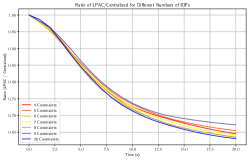
(b) Constraint Ablation. The performance ratio between LPAC and Centralized as a function of time for the fair coverage control problem. We vary the number of IDFs/constraints, from $4$ to $10$ IDFs with $1024\times 1024$ environment.

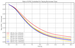
(c) Problem scale ablation. The performance ratio between LPAC and Centralized as a function of time in the fair coverage control problem. We vary the size of the environment and the number of robots, while maintaining the robot density.

Figure 4: Comparison of LPAC and Centralized performance under different experimental setups in the fair coverage control problem: robot ablation, feature ablation, and problem scale ablation.

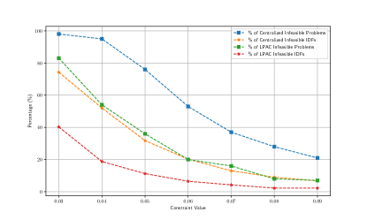
Figure 5: Contraint coverage control with varying constraint levels. We plot the IDF infeasibility and problem infeasibility (i.e. at least one IDF is infeasible) percentage.

In this section, we empirically study the two problems fair coverage and constrained coverage. The goals are to establish that the approach is: (i) an efficient solver for the multi-objective coverage control problem, (ii) generalization to a wide range of robot parameters, (iii) generalization to unseen domains, (iv) scales with number of robots, number of IDFs, and environment size.

We compare our method against four baseline controllers: decentralized and centralized CVT, SFCC [1], and the clairvoyant algorithm. The decentralized and centralized CVT algorithms operate on the partial information about the IDF gathered by the robots throughout the trajectory and utilize the combination of IDFs (see [2, Section V.A]). SFCC [1] is a centralized gradient-based algorithm that operates on the LogSumExp of the IDFs. The clairvoyant algorithm has perfect knowledge of all the IDFs and the positions of the robots and can, therefore, compute near-optimal actions for each robot. It is important to highlight that LPAC possesses the same local information as the decentralized CVT algorithm.

We begin by considering the fair coverage control problem (FMCP). Figure 1 presents the maximum coverage cost across all IDFs averaged over $100$ randomly generated environments. The LPAC outperforms centralized and decentralized CVT by $50\%$. Moreover, considering the standard deviation bands around each mean, we see that the centralized and LPAC fall outside the mean curve. The result illustrates the benefits of using GNNs for multi-objective coverage control, even when accessing partially decentralized information.

Figure 2 shows the performance of the LPAC algorithm with respect to the centralized solver as the communication radius and the sensor size of the robots are varied. The centralized algorithm is agnostic to the communication radius, and its performance increases with sensor size. The LPAC algorithm, on the other hand, is sensitive to the communication radius and the sensor size, and yet it consistently outperforms the centralized algorithm for all configurations.

In Figure 3, we plot the trajectories of the IDFs and the dual variables on the upper and lower rows, respectively. The upper row shows how the performance across IDFs improves as time progresses. The case of clairvoyant and LPAC present a switch on the most difficult IDF, from orange to green, at around $15$ time steps. In the case of the CVT algorithm, it struggles throughout all the trajectories with IDF orange. The value of the dual variable is proportional to the difficulty of satisfying the constraint, which, in this case, translates into minimizing that IDF. Therefore, the switch in the objective value also manifests as a switch in the maximum dual variable $\lambda$.

In terms of scalability, we run an ablation study on the number of robots from $8$ robots to $64$ in steps of $8$. Figure 4a shows the ablation study on the number of robots, in this case, we look at the ratio of the centralized controller by LPAC. We run $100$ experiments per number of robots and confirm that values are smaller than $1$ given that LPAC outperforms centralized CVT. We can see that when the number of robots is larger than $32$ (number of robots used for training), LPAC outperforms centralized CVT by more than $30\%$. Additionally, in Table I we show the number of times that each controller attains the best performance. Here the LPAC becomes even more useful given that LPAC performs better than centralized CVT at least $94\%$ of the time.

In Figure 4b run an ablation study on the number of IDFs or constraints, starting at $4$ and ending at $10$. In this case, we show the scalability in terms of the number of constraints, and we confirm that LPAC outperforms centralized CVT by at least $35\%$ in all cases. Thus showcasing the ability of LPAC to operate under a larger number of constraints.

In Figure 4c we scale the problem in the size of the environment and robots jointly. Once again, LPAC outperforms the centralized CVT algorithm by at least $35\%$, thus showing that LPAC scales in the coverage control problem size.

Constraint Coverage Control. We consider the constrained coverage control problem (CMCP). In this case, we compared the centralized CVT against our formulation of LPAC. Note that to the best of our knowledge, there does not exist another algorithm to compare against for the multi-objective coverage control problem. We considered the feasibility problem, i.e. $\phi_{0}=0$, and sampled the constraints $\alpha_{m}$ according to ${\mathcal{N}}(\mu,0.1)$, for $\mu\in\{0.3,\dots,0.9\}$, and considered $M=4$ IDFs.

In Figure 5 we plot the results, both in terms of the percentage of infeasible IDFs, as well as infeasible problems (at least one of the four IDFs is infeasible). As can be seen, the percentage of infeasible IDFs in LPAC is always less than half that in Centralized CVT. In terms of the problems, LPAC achieves an average of $25\%$ less infeasible problems across all $\mu$s. This showcases the benefits of our proposed approach for constrained multi-objective coverage control.

VI Conclusions

In this paper, we reformulate the multi-objective coverage control with constraints as a coverage control problem with a single objective. Our method relies on utilizing a dynamically re-weighted combination of maps using a dual algorithm. We showcased the benefits of our method by utilizing a decentralized learning technique based on Graph Neural Networks that abstracts the perceptions and learns the communications and actions to be taken by each robot based solely on local perception and communications. Empirically, we implemented a wide variety of experiments showcasing that our method is scalable—both in the number of importance fields, as well as in the number of robots in the swarm—and improves upon both centralized and decentralized CVT algorithms by an average of $30\%$. Future work involves real-world experiments in decentralized settings.

References

- [1] M. Malencia, G. Pappas, and V. Kumar, “Socially fair coverage control,” in 2023 IEEE International Conference on Robotics and Automation (ICRA), 2023, pp. 7656–7662.
- [2] S. Agarwal, R. Muthukrishnan, W. Gosrich, A. Ribeiro, and V. Kumar, “LPAC: Learnable perception-action-communication loops with applications to coverage control,” arXiv preprint arXiv:2401.04855, 2024.
- [3] B. Hexsel, N. Chakraborty, and K. Sycara, “Coverage control for mobile anisotropic sensor networks,” in IEEE International Conference on Robotics and Automation, 2011, pp. 2878–2885.
- [4] L. Doitsidis, S. Weiss, A. Renzaglia, M. W. Achtelik, E. Kosmatopoulos, R. Siegwart, and D. Scaramuzza, “Optimal surveillance coverage for teams of micro aerial vehicles in gps-denied environments using onboard vision,” Autonomous Robots, vol. 33, pp. 173–188, 2012.
- [5] L. C. Pimenta, M. Schwager, Q. Lindsey, V. Kumar, D. Rus, R. C. Mesquita, and G. A. Pereira, “Simultaneous coverage and tracking (scat) of moving targets with robot networks,” in Algorithmic Foundation of Robotics VIII: Selected Contributions of the Eight International Workshop on the Algorithmic Foundations of Robotics. Springer, 2010, pp. 85–99.
- [6] Cortés, Jorge, Martínez, Sonia, and Bullo, Francesco, “Spatially-distributed coverage optimization and control with limited-range interactions,” ESAIM: COCV, vol. 11, no. 4, pp. 691–719, 2005.
- [7] Q. Du, V. Faber, and M. Gunzburger, “Centroidal Voronoi Tessellations: Applications and Algorithms,” SIAM Review, vol. 41, no. 4, pp. 637–676, 1999.
- [8] H. Edelsbrunner and R. Seidel, “Voronoi diagrams and arrangements,” in Proceedings of the First Annual Symposium on Computational Geometry, ser. SCG ’85. New York, NY, USA: Association for Computing Machinery, 1985, p. 251–262.
- [9] S. Lloyd, “Least squares quantization in pcm,” IEEE Transactions on Information Theory, vol. 28, no. 2, pp. 129–137, 1982.
- [10] F. Gama, A. G. Marques, G. Leus, and A. Ribeiro, “Convolutional neural network architectures for signals supported on graphs,” IEEE Transactions on Signal Processing, vol. 67, no. 4, pp. 1034–1049, 2019.
- [11] R. Lam, A. Sanchez-Gonzalez, M. Willson, P. Wirnsberger, M. Fortunato, F. Alet, S. Ravuri, T. Ewalds, Z. Eaton-Rosen, W. Hu et al., “Graphcast: Learning skillful medium-range global weather forecasting,” arXiv preprint arXiv:2212.12794, 2022.
- [12] X. He, K. Deng, X. Wang, Y. Li, Y. Zhang, and M. Wang, “Lightgcn: Simplifying and powering graph convolution network for recommendation,” in Proceedings of the 43rd International ACM SIGIR conference on research and development in Information Retrieval, 2020, pp. 639–648.
- [13] A. Sanchez-Gonzalez, J. Godwin, T. Pfaff, R. Ying, J. Leskovec, and P. Battaglia, “Learning to simulate complex physics with graph networks,” in International conference on machine learning. PMLR, 2020, pp. 8459–8468.
- [14] M. Tzes, N. Bousias, E. Chatzipantazis, and G. J. Pappas, “Graph neural networks for multi-robot active information acquisition,” in 2023 IEEE International Conference on Robotics and Automation (ICRA). IEEE, 2023, pp. 3497–3503.
- [15] W. Gosrich, S. Mayya, R. Li, J. Paulos, M. Yim, A. Ribeiro, and V. Kumar, “Coverage control in multi-robot systems via graph neural networks,” in 2022 International Conference on Robotics and Automation (ICRA). IEEE, 2022, pp. 8787–8793.
- [16] E. Tolstaya, F. Gama, J. Paulos, G. Pappas, V. Kumar, and A. Ribeiro, “Learning decentralized controllers for robot swarms with graph neural networks,” in Conference on robot learning. PMLR, 2020, pp. 671–682.
- [17] Q. Li, F. Gama, A. Ribeiro, and A. Prorok, “Graph neural networks for decentralized multi-robot path planning,” in 2020 IEEE/RSJ international conference on intelligent robots and systems (IROS). IEEE, 2020, pp. 11 785–11 792.
- [18] Q. Li, W. Lin, Z. Liu, and A. Prorok, “Message-aware graph attention networks for large-scale multi-robot path planning,” IEEE Robotics and Automation Letters, vol. 6, no. 3, pp. 5533–5540, 2021.
- [19] Z. Wang, J. Cervino, and A. Ribeiro, “Generalization of graph neural networks is robust to model mismatch,” arXiv preprint arXiv:2408.13878, 2024.
- [20] F. Gama, J. Bruna, and A. Ribeiro, “Stability properties of graph neural networks,” IEEE Transactions on Signal Processing, vol. 68, pp. 5680–5695, 2020.
- [21] L. Ruiz, L. Chamon, and A. Ribeiro, “Graphon neural networks and the transferability of graph neural networks,” Advances in Neural Information Processing Systems, vol. 33, pp. 1702–1712, 2020.
- [22] Z. Wang, J. Cervino, and A. Ribeiro, “A manifold perspective on the statistical generalization of graph neural networks,” arXiv preprint arXiv:2406.05225, 2024.
- [23] L. F. Chamon, S. Paternain, M. Calvo-Fullana, and A. Ribeiro, “Constrained learning with non-convex losses,” IEEE Transactions on Information Theory, vol. 69, no. 3, pp. 1739–1760, 2022.
- [24] L. Chamon and A. Ribeiro, “Probably approximately correct constrained learning,” Advances in Neural Information Processing Systems, vol. 33, pp. 16 722–16 735, 2020.
- [25] Z. Shen, J. Cervino, H. Hassani, and A. Ribeiro, “An agnostic approach to federated learning with class imbalance,” in International Conference on Learning Representations, 2021.
- [26] A. Robey, L. Chamon, G. J. Pappas, H. Hassani, and A. Ribeiro, “Adversarial robustness with semi-infinite constrained learning,” Advances in Neural Information Processing Systems, vol. 34, pp. 6198–6215, 2021.
- [27] J. Cervino, L. F. Chamon, B. D. Haeffele, R. Vidal, and A. Ribeiro, “Learning globally smooth functions on manifolds,” in International Conference on Machine Learning. PMLR, 2023, pp. 3815–3854.
- [28] J. Elenter, N. NaderiAlizadeh, and A. Ribeiro, “A lagrangian duality approach to active learning,” Advances in Neural Information Processing Systems, vol. 35, pp. 37 575–37 589, 2022.
- [29] J. Cerviño, L. Ruiz, and A. Ribeiro, “Training stable graph neural networks through constrained learning,” in ICASSP 2022-2022 IEEE International Conference on Acoustics, Speech and Signal Processing (ICASSP). IEEE, 2022, pp. 4223–4227.
- [30] R. Arghal, E. Lei, and S. S. Bidokhti, “Robust graph neural networks via probabilistic lipschitz constraints,” in Learning for Dynamics and Control Conference. PMLR, 2022, pp. 1073–1085.
- [31] S. Paternain, M. Calvo-Fullana, L. F. Chamon, and A. Ribeiro, “Safe policies for reinforcement learning via primal-dual methods,” IEEE Transactions on Automatic Control, vol. 68, no. 3, pp. 1321–1336, 2022.
- [32] A. Castellano, H. Min, E. Mallada, and J. A. Bazerque, “Reinforcement learning with almost sure constraints,” in Learning for Dynamics and Control Conference. PMLR, 2022, pp. 559–570.
- [33] S. Rozada, D. Ding, A. G. Marques, and A. Ribeiro, “Deterministic policy gradient primal-dual methods for continuous-space constrained mdps,” arXiv preprint arXiv:2408.10015, 2024.
- [34] Y. Kim, H. Oh, J. Lee, J. Choi, G. Ji, M. Jung, D. Youm, and J. Hwangbo, “Not only rewards but also constraints: Applications on legged robot locomotion,” IEEE Transactions on Robotics, 2024.
- [35] M. De Berg, Computational geometry: algorithms and applications. Springer Science & Business Media, 2000.
- [36] S. Boyd and L. Vandenberghe, Convex optimization. Cambridge university press, 2004.
- [37] J. Elenter, L. F. Chamon, and A. Ribeiro, “Near-optimal solutions of constrained learning problems,” in The Twelfth International Conference on Learning Representations, 2024.
- [38] S. Ioffe and C. Szegedy, “Batch normalization: Accelerating deep network training by reducing internal covariate shift,” in Proceedings of the 32nd International Conference on International Conference on Machine Learning - Volume 37, ser. ICML’15. JMLR.org, 2015, p. 448–456.
- [39] L. Ruiz, F. Gama, and A. Ribeiro, “Graph neural networks: Architectures, stability, and transferability,” Proceedings of the IEEE, vol. 109, no. 5, pp. 660–682, 2021.
- [40] D. Kingma and J. Ba, “Adam: A method for stochastic optimization,” in International Conference on Learning Representations (ICLR), San Diega, CA, USA, 2015.
- [41] A. Paszke, S. Gross, F. Massa, A. Lerer, J. Bradbury, G. Chanan, T. Killeen, Z. Lin, N. Gimelshein, L. Antiga, A. Desmaison, A. Kopf, E. Yang, Z. DeVito, M. Raison, A. Tejani, S. Chilamkurthy, B. Steiner, L. Fang, J. Bai, and S. Chintala, “PyTorch: An Imperative Style, High-Performance Deep Learning Library,” in Advances in Neural Information Processing Systems 32, H. Wallach, H. Larochelle, A. Beygelzimer, F. d’Alché Buc, E. Fox, and R. Garnett, Eds. Curran Associates, Inc., 2019, pp. 8024–8035.
- [42] M. Fey and J. E. Lenssen. (2019, May) Fast Graph Representation Learning with PyTorch Geometric.