An Extended Variational Method for the Resistive Wall Mode in Toroidal Plasma Confinement Devices
Abstract
The external-kink stability of a toroidal plasma surrounded by a rigid resistive wall is investigated. The well-known analysis of Haney & Freidberg is rigorously extended to allow for a wall that is sufficiently thick that the thin-shell approximation does not necessarily hold. A generalized Haney-Freidberg formula for the growth-rate of the resistive wall mode is obtained. Thick-wall effects do not change the marginal stability point of the mode, but introduce an interesting asymmetry between growing and decaying modes. Growing modes have growth-rates that exceed those predicted by the original Haney-Freidberg formula. On the other hand, decaying modes have decay-rates that are less than those predicted by the original formula.
The well-known Hu-Betti formula for the rotational stabilization of the resistive wall mode is also generalized to take thick-wall effects into account. Increasing wall thickness facilitates the rotational stabilization of the mode, because it decreases the critical toroidal electromagnetic torque that the wall must exert on the plasma. On the other hand, the real frequency of the mode at the marginal stability point increases with increasing wall thickness.
I Introduction
According to standard ideal-magnetohydrodynamical (ideal-MHD) stability theory, a fusion plasma confined on a set of toroidally nested magnetic flux-surfaces can be rendered completely stable to ideal external-kink modes by means of a perfectly conducting, rigid wall that is located sufficiently close to the plasma boundary.ek1 ; ek2 ; ek3 Of course, a practical metal wall possesses a finite electrical conductivity, and can, therefore, only act as a perfect conductor on timescales that are much less than its characteristic L/R time. Given that the L/R time of any conceivable wall ( s) is considerably smaller than the desired confinement time of a fusion plasma ( s),tok ; fit it is clear that the finite conductivity of the wall must be taken into account in the stability analysis. When the finite wall conductivity is taken into consideration, ideal external-kink modes that would be stabilized by the wall, were it perfectly conducting, are found to grow on the L/R time of the wall.rwm1 ; rwm2 Such comparatively slowly growing modes [compared to ideal external-kink modes, which grow on the extremely short ( s) Alfvén time] bern ; freid ; freid1 ; goed are known as resistive wall modes. In 1989, Haney & Freidberg hf derived a very general formula for the growth-rate of a resistive wall mode that makes use of the “thin-shell approximation”, according to which the skin depth in the wall material is assumed to be much larger than the wall thickness. The aim of this paper is to generalize the Haney-Freidberg formula to allow for thicker walls in which the thin-shell approximation breaks down.thick0 ; thick01 ; chap ; thick1 ; thick2 ; thick3 ; thick4 A secondary aim of the paper is to elucidate some subtleties in resistive wall mode theory.
II Ideal External-Kink Mode Stability
II.1 Introduction
This section summarizes some well-known background material.
II.2 Scenrario
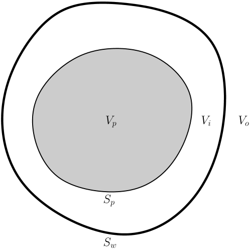
Consider a fusion plasma that is confined on a set of toroidally-nested magnetic flux-surfaces. Let represent the toroidal volume occupied by the plasma, and let be the volume’s bounding surface. Suppose that the plasma is surrounded by a rigid, conducting wall whose uniform thickness, , is small compared to its effective minor radius, . Let the wall occupy the toroidal surface . Let represent the vacuum region lying between the plasma boundary and the wall. Finally, let represent the vacuum region that lies outside the wall, and extends to infinity. See Fig. 1.
II.3 Plasma Equilibrium
Let , , , and represent the equilibrium plasma mass density, scalar pressure, magnetic field, and electric current density, respectively. It follows that , and . Let be a unit, outward directed normal vector to . We have
| (1) |
on , because must correspond to a magnetic flux-surface. We also expect the rapid transport of particles and energy along magnetic field-lines to ensure that fit
| (2) |
on . Hence, we deduce from the equilibrium force balance equation that
| (3) |
on . Finally, equilibrium force balance across yields
| (4) |
on , which implies that
| (5) |
on . Here, is the equilibrium magnetic field in the vacuum region.
II.4 Plasma Perturbation
Assuming an time dependence of all perturbed quantities, and neglecting equilibrium plasma flows, the perturbed, linearized plasma equation of motion takes the form bern ; freid ; freid1 ; goed
| (6) |
where
| (7) |
and
| (8) |
Here, is the plasma displacement, the ratio of specific heats, and the divergence-free perturbed magnetic field in the plasma. Moreover, is known as the force operator. The divergence-free perturbed magnetic field in the vacuum region is written , where
| (9) |
Now, must be square integrable at the magnetic axis, otherwise the potential energy, [see Eq. (19)], of the perturbation would be infinite. Furthermore,freid ; freid1 ; goed
| (10) | ||||
| (11) |
on . Equation (10) ensures that the perturbed plasma boundary remains a magnetic flux-surface, whereas Eq. (11) is an expression of perturbed pressure balance across the boundary. Finally, if the wall is perfectly conducting then
| (12) |
on , where is a unit, outward directed normal vector to . On the other hand, if the wall is absent then
| (13) |
at infinity. Equation (12) ensures that the perturbed magnetic field cannot penetrate the perfectly conducting wall, whereas Eq. (13) ensures that the potential energy of the perturbation remains finite. The boundary conditions (10), (12), and (13), as well as the constraint that be square integrable at the magnetic axis, and the constraint that be square integrable at infinity, are conventionally termed essential boundary conditions, whereas the boundary condition (12) is termed a natural boundary condition.freid ; freid1 ; goed An essential boundary condition is one that must be satisfied by all prospective solution pairs, [, ]. On the other hand, a natural boundary condition is one that must be satisfied by physical solution pairs, but, as we shall see, can be violated by trial solution pairs.
II.5 Self-Adjoint Property of Force Operator
Let [, ] and [, ] be two independent prospective solution pairs that satisfy both the essential and the natural boundary conditions. It is easily demonstrated that goed
| (14) |
where , and use has been made of Eqs. (1)–(3). The surface integral can be expressed as
| (15) |
where use has been made of Eqs. (5), (10), and (11). However, the boundary conditions (12) and (13) allow us to write
| (16) |
where use has been made of Eq. (9). Here, denotes the appropriate vacuum region: i.e., for the case of a perfectly conducting wall, and for the case of no wall. The previous three equations yield
| (17) |
The well-known self-adjoint property of the force operator,bern ; freid ; freid1 ; goed
| (18) |
immediately follows from the invariance of Eq. (II.5) under the transformation , , , , , respectively.
II.6 Ideal-MHD Energy Principle
The potential energy of the perturbation characterized by the solution pair [, ] takes the form bern ; freid ; freid1 ; goed
| (19) |
It follows from Eq. (II.5) that
| (20) |
where
| (21) | ||||
| (22) | ||||
| (23) |
Clearly, , , and respectively represent the contributions from the bulk plasma, from equilibrium surface currents flowing on the plasma boundary, and from the vacuum, to the overall potential energy of the perturbation.
The ideal-MHD energy principle bern ; freid ; freid1 ; goed states that if any solution pair that satisfies the boundary conditions makes then the plasma is ideally unstable. In other words, at least one eigenmode with exists, where is of order the inverse Alfvén time. On the other hand, if no valid solution pair can be found such that then the plasma is ideally stable. In other words, all eigenmodes are characterized by .
Clearly, in order to utilize the ideal-MHD principle, we need to minimize with respect to , and then determine whether the minimum value is positive or negative. In the former case, the plasma is ideally stable. In the latter case, it is ideally unstable. We can write
| (24) |
where use has been made of the self-adjoint property of the force operator, (18). It is easily demonstrated that
| (25) | ||||
| (26) | ||||
| (27) |
Here, use has been made of the boundary conditions (10), (12), and (13), which are assumed to apply to and . Thus, setting , we get
| (28) |
Because the previous equation must hold for arbitrary and , we deduce that the trial solution pair that minimizes satisfies the force-balance equation,
| (29) |
in , satisfies Eq. (9) in , and also ought to satisfy the pressure balance matching condition, (11), at the plasma boundary.
II.7 Perfect-Wall and No-Wall Stability
Suppose that the wall is perfectly conducting. In this case, the previous analysis suggests that the minimum value of the perturbed potential energy can be written
| (30) |
where and are calculated from a particular solution of Eq. (29) that is well-behaved at the magnetic axis, and
| (31) |
Here, the superscript implies that the perfectly conducting wall is present at effective minor radius . Moreover, is a solution of Eq. (9) that satisfies the boundary conditions
| (32) |
on [see Eq. (10)], and
| (33) |
on . [See Eq. (12).] We can be sure that if then the ideal external-kink mode in question is stabilized by the wall.
Suppose that there is no wall. In this case, the previous analysis suggests that the minimum value of the perturbed potential energy can be written
| (34) |
where and are calculated from the same solution of Eq. (29) as that used to calculate , and
| (35) |
Here, the superscript implies that the perfectly conducting wall is absent, which is equivalent to it being placed at infinity. Moreover, is a solution of Eq. (9) that satisfies the boundary conditions
| (36) |
on [see Eq. (10)], and
| (37) |
at infinity. [See Eq. (13).] We can be sure that if then the ideal external-kink mode in question is unstable in the absence of the wall. Of course, the situation in which a kink mode is unstable in the absence of the wall, and stable in the presence of perfectly conducting wall, is exactly that which pertains to the resistive wall mode.
II.8 Discussion
The reason that we have reproduced the very standard theory outlined in Sects. II.3–II.7 is to make an important observation. Namely, the solution pairs, [, ] and [, ], conventionally used to calculate and , respectively, do not satisfy the pressure balance matching condition, (11), at the plasma boundary. One way of seeing this is to note that if in then, according to Eq. (19), . However, if we assume that the pressure balance matching condition is not satisfied then Eq. (20) generalizes to
| (38) |
where
| (39) |
Here, the surface energy is directly related to the failure to satisfy the pressure balance matching condition at the plasma boundary. Thus, it is clear that
| (40) | ||||
| (41) |
In other words, the only reason that and can take non-zero values at all is because the pressure balance matching condition is not satisfied. See Sect. IV.12.
The fact that the the solution pairs, [, ] and [, ], do not satisfy the pressure balance matching condition, (11), at the plasma boundary is not problematic within the context of ideal-MHD theory. The ideal-MHD energy principle guarantees that if then we can find a solution of Eq. (6) inside the plasma, and Eq. (9) outside the plasma, which satisfies all of the boundary conditions in the absence of a wall, and is such that . Likewise, if then we can find a solution of Eq. (6) inside the plasma, and Eq. (9) outside the plasma, which satisfies all of the boundary conditions in the presence of a perfectly conducting wall, and is such that . In both cases, the undetermined Alfvénic growth-rate of the instability, , provides the additional degree of freedom that allow the pressure balance matching condition, (11), to be satisfied at the plasma boundary. However, the analysis of Haney-Freidberg constructs the resistive wall mode solution from a linear combination of [, ] and [, ]. Moreover, such a solution must satisfy all of the boundary conditions, including Eq. (11). Thus, it is important to demonstrate that this is actually possible.
III Resistive Wall Mode Physics
III.1 Resistive Wall Physics
Let be the vector potential in . Let be the vector potential in . Finally, let be the vector potential inside the wall. Choosing the Coulomb gauge within the wall,jackson the electric field in the wall takes the form
| (42) |
whereas the magnetic field is given by
| (43) |
Ohm’s law inside the wall yields
| (44) |
where is the uniform electrical conductivity of the wall material, and is the density of the electrical current flowing in the wall. Finally,
| (45) |
The previous four equations can be combined to give
| (46) |
Let and be the uniform thickness and effective minor radius of the wall, respectively. Now, we are assuming that the wall is physically thin: i.e., . Following Haney & Freidberg,hf the position vector of a point lying within the wall is written
| (47) |
where is the position vector of a point on the inner surface of the wall. The normalized length represents perpendicular distance measured outward from the inner surface of the wall. Thus, and correspond to the inner and outer surface of the wall, respectively. We deduce that the gradient operator within the wall can be written
| (48) |
where only involves derivatives tangent to the surface of the wall.
To lowest order in , Eqs. (46) and (48) yield
| (49) |
where
| (50) |
Let
| (51) |
The neglect of tangential derivates with respect to perpendicular derivatives in Eq. (49) is valid as long as
| (52) |
which we shall assume to be the case. Note that
| (53) |
where
| (54) |
is the skin depth in the wall material.jackson The so-called thin-shell limit correspond to the situation in which the skin depth is much greater than the wall thickness: i.e., . On the other hand, the thick-shell limit corresponds to the situation in which the skin depth is greater than or comparable to the wall thickness: i.e., . Note that it is possible for the wall to be physically thin (i.e., ) but still be in the thick-shell limit.
Equation (49) yields
| (55) |
The solution is
| (56) |
where is an arbitrary constant. Here, we have made the simplifying assumption that does not change direction across the wall: i.e., as varies from 0 to 1. This assumption is certainly valid in the thin-shell limit, and we shall assume that it is also valid in the thick-shell limit. To lowest order in ,
| (57) |
The boundary conditions that must be satisfied at the inner and outer surfaces of the wall are continuity of the tangential component of the electric field,jackson and continuity of the tangential component of the magnetic field. The latter boundary condition follows because we are assuming that there are no sheet currents flowing on the inner or the outer surface of the wall.hf Thus, we obtain
| (58) | ||||
| (59) | ||||
| (60) | ||||
| (61) |
where use has been made of Eqs. (51), (56), and (57). Here, and are evaluated on the inner and outer surfaces of the wall, respectively.
Let
| (62) |
Note that must be a scalar in order to satisfy Eq. (61). Now, we expect to decay monotonically to zero as we move from the outer surface of the wall to infinity. Moreover, we expect the decay length to be of order . It follows that .
Equations (61) and (62) can be combined to give
| (63) |
It follows that chap
| (64) |
To lowest order in , Eqs. (59), (60), and (62) yield
| (65) | ||||
| (66) |
The previous equation gives
| (67) |
Equations (65) and (66) [or, alternatively, Eq. (67)] are the two matching conditions that must be satisfied at the wall. According to Eq. (65), in the thin-shell limit.hf On the other hand, in the thick-shell limit, due to the shielding of the outer vacuum region, , from the inner vacuum region, , by eddy currents excited in the wall. Finally, Eqs. (65) and (67) can be combined to produce
| (68) |
III.2 Timescale Ordering
In order for the left-hand side of Eq. (6) to compete with the right-hand side, we need , where s. Here, is the minor radius of the plasma. However, the growth-rate of a resistive wall mode is of order s.rwm1 ; rwm2 ; hf Hence, it is clear that, for the case of a resistive wall mode, the left-hand side of Eq. (6) is negligible. In other words, plasma inertia is negligible. Consequently, the plasma displacement associated with the resistive wall mode satisfies the force balance equation, (29), within the plasma. Note that we are saying that the actual physical solution, as opposed to a trial solution, must satisfy Eq. (29) within the plasma.
III.3 Self-Adjoint Property of Force Operator
We wish to prove that the force operator remains self-adjoint in the presence of a resistive wall. The proof follows along the lines of that outlined in Sect. II.5, except that
| (69) |
where use has been made of Eq. (9). However, Eq. (68) can easily be generalized to give
| (70) |
Moreover,
| (71) |
where use has been made of Eqs. (9) and (13). Hence, we deduce that
| (72) |
Thus, in the presence of a resistive wall, Eq. (II.5) generalizes to give
| (73) |
The self-adjoint property of the force operator, (18), immediately follows from the symmetric nature of the previous equation. Thus, we conclude that the force operator remains self-adjoint in the presence of a resistive wall, even when the wall lies in the thick-shell limit.
III.4 Variational Principle
Making use of the previous equation, the perturbed potential energy of the resistive wall mode can be written
| (74) |
where
| (75) | ||||
| (76) | ||||
| (77) |
Clearly, is the potential energy associated with the vacuum region interior to the wall, is the potential energy associated with the vacuum region exterior to the wall, and is the potential energy associated with eddy currents excited in the wall. In fact, it is easily demonstrated that
| (78) |
where represents the volume occupied by the wall. In deriving the previous formula, we have assumed that in , which implies that the eddy currents excited in the wall flow predominately in directions tangental to the wall surface (because ). Incidentally, it is easily demonstrated that the magnetic energy of the wall, , is negligible.
Given that Eq. (29) holds within the plasma, it is clear that from Eq. (19) that
| (79) |
for a resistive wall mode. This is not a surprising result, because a resistive wall mode is essentially a marginally stable ideal mode (given that ), which corresponds to a mode with .
Consider
| (80) |
where use has been made of the self-adjoint property of the force operator, (18). Now, and are again given by Eqs. (II.6) and (26), respectively. Moreover,
| (81) |
where use has been made of the essential boundary condition (10). Furthermore,
| (82) |
where use has been made of the essential boundary condition (13), as well as Eq. (65). Finally,
| (83) |
Thus, setting to zero, we obtain
| (84) |
However, the previous equation must hold for arbitrary and . Hence, we deduce that the solution pair, [, , that minimizes the specified in Eq. (75) satisfies Eq. (29) in , satisfies Eq. (9) in and , satisfies the pressure balance matching condition, (11), at the plasma boundary, and satisfies the matching condition (67) at the wall. In other words, the solution pair solves the resistive wall mode problem.
Note that the wall matching condition (65) is clearly an essential boundary condition, whereas the matching condition (66) [or, alternatively, (67)] plays the role of a natural boundary condition.freid1
We might ask why we believe that the solution pair that minimizes the specified in Eq. (75) will satisfy the pressure balance matching condition, (11), at the plasma boundary, when the solution pair that minimizes the specified in Eq. (20) failed to do this. The answer is that the unspecified growth-rate of the resistive wall mode, , introduces an additional degree of freedom into the system that allows us to simultaneously satisfy all of the boundary conditions.
III.5 Generalized Haney-Freidberg Formula
Following Haney & Freidberg,hf let us write
| (85) | ||||
| (86) |
where , , and are constants that must be determined by the essential boundary conditions and the minimization process. Now, the essential boundary condition (10) implies that
| (87) |
on . Combining this relation with Eqs. (32), (36), and (85), we deduce that
| (88) |
Next, the essential boundary condition (65) can be combined with Eqs. (33), (85), and (86) to give
| (89) |
Note that the essential boundary condition (13) is automatically satisfied because of Eq. (37).
The following results are easily demonstrated:
| (90) | ||||
| (91) | ||||
| (92) | ||||
| (93) |
and
| (94) |
where use has been made of Eqs. (9), (10), (12), (13), (32), (33), (36), (37), (85), and (86). It is helpful to define
| (95) |
Here, represents the contribution of the region to the no-wall vacuum energy. The previous eight equations can be combined to the give the following expression for the vacuum energy:
| (96) |
Now, the ratio of the first term to the second term appearing in square brackets in the previous equation is
| (97) |
Thus, in the thin-shell limit, , the ratio is , which is very large. On the other hand, in the thick-shell limit, , the ratio is [see Eq. (51)], which is also very large. Hence, we deduce that we can neglect the second term. Thus, the previous equation simplifies to give
| (98) |
where
| (99) |
According to the variational principle proved in Sect. III.4, we can determine the true vacuum energy by minimizing with respect to variations in . This procedure yields
| (100) | ||||
| (101) |
Following Haney & Freidberg,hf we can define the effective minor radius of the wall as
| (102) |
| (103) |
where
| (104) | ||||
| (105) | ||||
| (106) |
Here, is the effective L/R time of the wall, whereas measures the relative wall thickness.
According to Eqs. (75), (III.5), and (103), the total potential energy of the perturbation is
| (107) |
where use has been made of Eqs. (30) and (34). Finally, Eq. (79) mandates that for a resistive wall mode, so we obtain the following generalized Haney-Freidberg formula:
| (108) |
for the case , in which the resistive wall mode is unstable, and
| (109) |
for the case , in which the resistive wall mode is stable. The formula does not apply to the case in which the plasma is ideally unstable in the presence of the wall, because the neglect of plasma inertia is not tenable in this situation. The derivation of the generalized Haney-Freidberg formula is valid provided
| (110) |
In the thin-shell limit, , Eqs. (108)–(109) reduce to the original Haney-Freidberg formula:
| (111) |
Equations (79), (88), (100), and (107) yield
| (112) | ||||
| (113) |
Moreover, given that the gereralized Haney-Freidberg dispersion relation sets , a comparison of Eqs. (38) and (107) reveals that , where is defined in Eq. (II.8). Thus, it is plausible that the linear combination of solutions, (85), with and given by the previous two equations, ensures that the pressure balance matching condition, (11), is satisfied at the plasma boundary. Later on, in Sect. IV.14, we shall show this explicitly.
III.6 Resistive Wall Mode Growth-Rate
Figure 2 shows the growth-rate of the resistive wall mode predicted by the generalized Haney-Freidberg formula, (108)–(109). For a thin wall characterized by , we reproduce the characteristic linear relationship between and predicted by the original Haney-Freidberg formula. The mode grows or decays on the characteristic L/R timescale, , and the marginal stability point, , is the same as that for an ideal-kink mode in the absence of a wall. Thick-wall effects, which manifest themselves when , do not change the marginal stability point, but introduce an interesting asymmetry between growing and decaying modes. Growing modes have growth-rates that exceed those predicted by the original Haney-Freidberg formula. (Here, we are comparing thick and thin walls with the same values.) On the other hand, decaying modes have decay-rates that are less than those predicted by the original formula. Note that there are actually multiple branches of decaying solutions, and we have plotted the most slowly decaying branch in Fig. 2.
For a very rapidly growing resistive wall mode, such that , which corresponds to the complete breakdown of the thin-shell approximation, Eq. (108) reduces to thick0 ; thick2
| (114) |
In this limit, the mode is almost completely shielded from the vacuum region outside the wall. [See Eq. (65).] According to Eq. (109), a very rapidly decaying resistive wall mode (on the slowest decaying solution branch) cannot decay faster than
| (115) |
Interestingly, rapidly growing resistive wall modes only partially penetrate the wall (in other words, the skin-depth in the wall material is much less than the wall thickness), whereas rapidly decaying modes always penetrate the wall (in other words, the skin-depth in the wall material is of order the wall thickness).
III.7 Further Generalization of Haney-Freidberg Formula
Our analysis has assumed that the thickness, , and conductivity, , of the wall are uniform. However, if we redo the previous analysis without making this assumption then very similar arguments reveal that
| (116) |
where both and , which appear inside the expressions for and [see Eqs. (105) and (106)], are now allowed to vary around the wall.
IV Axisymmetric Quasi-Cylindrical Equilibrium
IV.1 Introduction
In order to further illustrate some of the arguments presented in this paper, let us calculate the resistive wall stability of an axisymmetric toroidal plasma of major radius that is modeled as a periodic cylinder. Let , , be right-handed cylindrical coordinates. Let the magnetic axis of the plasma corresponds to , and let the cylinder be periodic in the -direction, with periodicity length .
IV.2 Plasma Equilibrium
The plasma equilibrium is such that and . Force balance within the plasma yields
| (117) |
where . Force balance across the plasma boundary, which lies at , demands that
| (118) |
at . In the vacuum region, , we have and .
IV.3 Perturbation
Let us assume that all perturbed quantities vary with and as , where is the poloidal mode number of the instability, , and is the toroidal mode number. The plasma displacement is written
| (119) |
where , and . Here, is assumed to be real, whereas and turn out to be imaginary. Note that , , and form a right-handed set of mutually orthogonal unit vectors.
IV.4 Plasma Potential Energy
The perturbed plasma potential energy can be written freid ; freid1 ; goed
| (120) |
where , , and the factor comes from averaging . After a great deal of standard analysis, we arrive at
| (121) |
where
| (122) |
and
| (123) | ||||
| (124) | ||||
| (125) | ||||
| (126) | ||||
| (127) | ||||
| (128) |
Because and only appear in Eq. (IV.4) inside positive-definite terms, we can minimize by choosing and in such a manner as to set these terms to zero. After doing this, and after integrating by parts, we arrive at freid ; freid1 ; goed ; new
| (129) |
where
| (130) | ||||
| (131) |
IV.5 Surface Potential Energy
The perturbed potential energy associated with equilibrium surface currents can easily be shown to take the form
| (132) |
IV.6 Vacuum Region
We shall write the divergence- and curl-free perturbed magnetic field in the vacuum region as
| (133) |
Here, , where is assumed to be real. Now, the wall matching condition (65) implies that . Hence, we deduce that
| (134) | ||||
| (135) | ||||
| (136) |
IV.7 Matching Conditions at Plasma Boundary
IV.8 Matching Conditions at Wall
The wall is assumed to be uniform, and located at minor radius . Given that , the essential boundary condition (65) gives
| (139) |
Moreover, the natural boundary condition (66) reduces to
| (140) |
Here, and denote the inner and outer wall radii, respectively, where it is assumed that the wall is radially thin. Furthermore, .
IV.9 Vacuum Potential Energy
The contribution of the vacuum region lying internal to the wall to the overall potential energy of the perturbation can be shown to be [see Eqs. (75) and (133)]
| (141) |
where use has been made of the essential boundary condition (137). Similarly, the contribution of the vacuum region lying outside the wall is [see Eqs. (76) and (133)]
| (142) |
IV.10 Wall Potential Energy
IV.11 Variation Principle
The total potential energy of the perturbation is
| (144) |
Here, use has been made of the essential boundary condition (139). If we minimize the potential energy, making use of the previously demonstrated self-adjoint property of the overall expression, then we get
| (145) |
Given that the previous expression must hold for arbitrary and , we deduce that the perturbation that minimizes satisfies Newcomb’s equation,new
| (146) |
in the plasma, satisfies
| (147) |
in the vacuum, and satisfies the natural boundary conditions (138) and (140) at the plasma boundary and at the wall, respectively.
IV.12 No-Wall and Perfect-Wall Energies
The independent solutions of Eq. (147) are and , where and are modified Bessel functions. The vacuum scalar potential associated with the no-wall solution must satisfy
| (148) |
at the plasma boundary [see Eq. (137)], and
| (149) |
at infinity. [See Eq. (37).] It follows that
| (150) |
Here, ′ denotes differentiation with respect to argument. The vacuum potential energy associated with the no-wall solution is
| (151) |
where use has been made of Eqs. (75), (133), (137), (147), and (149).
The vacuum scalar potential associated with the perfect-wall solution must satisfy
| (152) |
at the plasma boundary [see Eq. (137)], and
| (153) |
at the wall. [See Eq. (33).] It follows that
| (154) |
The vacuum potential energy associated with the perfect-wall solution is
| (155) |
where use has been made of Eqs. (75), (133), (137), (147), and (153).
Now, integrating by parts, and making use of Eq. (146), the expression, (129), for the plasma potential energy becomes
| (156) |
Thus, the total potential energy of the no-wall ideal external-kink mode takes the form
| (157) |
Likewise, the total potential energy of the perfect-wall ideal external-kink mode can be written
| (158) |
In accordance with the discussion in Sect. II.8, we can see that the only reason that the energies and can take non-zero values is because the solution pairs, , , from which they are constructed, do not satisfy the pressure balance matching condition, (138), at the plasma boundary.
IV.13 Effective Wall Radius
IV.14 Pressure Balance Matching Condition
Let
| (162) |
According to Eqs. (112), (113), (IV.12), and (IV.12),
| (163) | ||||
| (164) |
Thus, the linear combination of solutions that satisfies the resistive wall mode problem is characterized by [see Eq. (85)]
| (165) |
However, the pressure balance matching condition at the plasma boundary, (138), can be written
| (166) |
Thus, it is clear that the matching condition is satisfied when the growth-rate of the resistive wall mode takes the correct value, which is specified by [see Eqs. (105), (106), (108), and (109)],
| (167) |
Here, is the true time-constant of the wall, and is a measure of its true thickness.
IV.15 Force-Free Reversed-Field Pinch Equilibrium
Consider a reversed-field pinch freid1 plasma equilibrium. Let us assume, for the sake of simplicity, that the equilibrium pressure is negligible. In this case, the equilibrium magnetic field, both in the plasma and in the vacuum, satisfies slinky
| (168) | ||||
| (169) |
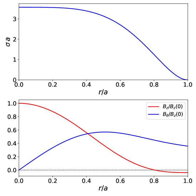
where . Let us adopt the following model profile,slinky
| (170) |
where , . Note that , which implies that there is no equilibrium current sheet flowing around the plasma boundary.
The resistive wall mode perturbation can be specified, both in the plasma and in the vacuum, in terms of the perturbed poloidal flux, ,fit where
| (171) |
The matching condition (137) becomes
| (172) |
whereas the pressure balance matching condition, (138), reduces to
| (173) |
Note that a failure to satisfy the pressure balance matching condition is associated with a gradient discontinuity in at the plasma boundary. Such a discontinuity implies the existence of a perturbed current sheet flowing on the boundary.
Inside the plasma, Newcomb’s equation, (146), can be re-expressed in the form slinky
| (174) |
where
| (175) | ||||
| (176) |
Note that Eq. (174) is singular at any equilibrium magnetic flux-surface, , lying within the plasma, that satisfies . An ideal solution (which is unable to reconnect magnetic field-lines) must satisfy at such a surface.freid1 ; fit It is helpful to define
| (177) |
where is a solution of Eq. (174) that is well-behaved at , satisfies at any singular surfaces within the plasma, and is such that . Thus, the solution in the region becomes
| (178) |
where , which is the value of the perturbed poloidal magnetic flux at the plasma boundary, is undetermined.
Outside the plasma, in the region , we can write
| (179) |
where , and . [See Eqs. (186) and (187).] This automatically satisfies the matching condition (174). Here,
| (180) | ||||
| (181) |
Note that , in accordance with Eqs. (149) and (153). Furthermore, it is understood that . It is helpful to define
| (182) | ||||
| (183) |
It is easily demonstrated that
| (184) | ||||
| (185) |
Furthermore,
| (186) | ||||
| (187) |
Note that .
IV.16 Example Calculation
Let us adopt the following equilibrium parameters: , , , and . The resulting generic reversed-field pinch equilibrium is shown in Fig. 3. The characteristic pinch and reversal parameters freid1 are and , respectively. As is well-known, it is necessary to place the wall relatively close to a reversed-field pinch plasma in order to stabilize all possible ideal external-kink modes.freid1 In the present case, we choose . The thickness of the wall is , which is the largest value that we could adopt and plausibly argue that .
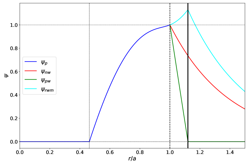
Consider the resistive wall mode. This is a mode that possesses a resonant surface in the plasma located at . The no-wall and perfect-wall energies of the mode are and , respectively. The fact that both energies are positive indicates that the mode is stable. In fact, the decay-rate of the mode is . If the wall were in the thin-shell limit, but had the same value, then the decay-rate would have been . Thus, the finite thickness of the wall has decreased the decay-rate of mode, in accordance with the discussion in Sect. III.6. However, despite the comparatively large wall thickness, the reduction is extremely modest.
Figure 4 shows the eigenfunctions of the resistive wall mode. The no-wall ideal external-kink mode has the eigenfunction , , where the first function corresponds to the plasma, whereas the second corresponds to the vacuum. It can be seen that this eigenfunction has a gradient discontinuity at the plasma boundary, indicating that it does not satisfy the pressure balance matching condition. The perfect-wall ideal external-kink mode has the eigenfunction , . Again, this eigenfunction has a gradient discontinuity at the plasma boundary, indicating that it does not satisfy the pressure balance matching condition. Finally, the resistive wall mode has the eigenfunction , . Note that this eigenfunction is completely continuous across the plasma boundary, indicating that it does satisfy the pressure balance matching condition.
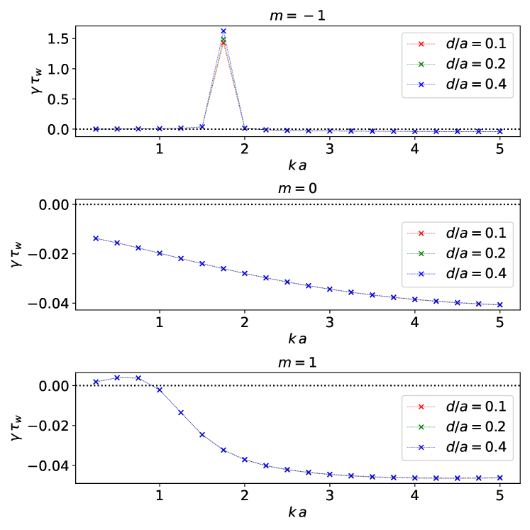
Figure 5 shows the growth-rates of the , , and resistive wall modes, calculated for in the range 1 to 20, and for various values of the wall thickness. It can be seen that the varying wall thickness makes no discernible difference to the growth-rates of the modes, with the exception of the mode. It turns out that the ideal external-kink mode is barely stabilized by a perfectly-conducting wall located at . Consequently, the corresponding resistive wall mode has a comparatively large growth-rate. In fact, in this case, it can be seen that increasing wall thickness (at fixed ) leads to a noticeable increase in the growth-rate, in accordance with the discussion in Sect. III.6. Thus, we conclude that thick-wall effects are only important for resistive wall modes that lie fairly close to the perfect-wall ideal stability boundary.
V Rotational Stabilization of Resistive Wall Mode
V.1 Generalized Hu-Betti Formula
So far, the analysis presented this paper suggests that the marginal stability point for the resistive wall mode is the same as that for the no-wall ideal external-kink mode: that is, . In other words, a close-fitting resistive wall is capable of transforming a rapidly growing ideal external-kink mode into a slowly growing resistive wall mode, but is unable to completely stabilize the mode.freid1 This conclusion is ultimately a consequence of the fact that the plasma potential energy, , is a real quantity. However, it turns out that resonances within the plasma, in combination with toroidal plasma rotation, allow to acquire an imaginary component.res1 The resonances in question include resonances with the sound wave continuum,res2 resonances with the shear-Alfvén wave continuum,res3 and resonances with trapped and circulating particles.res4 ; res5 Furthermore, above a critical plasma rotation rate, the resistive wall mode is stabilized by the imaginary component of .bond
Let us write
| (190) |
where and are the real and imaginary components of , respectively. We can then make the following redefinitions:
| (191) | ||||
| (192) |
Incidentally, it is obvious, from their definitions, that , , and are all real quantities. Note that the real part of the resonant contribution to has been incorporated into . Generally speaking, we expect to be proportional to the toroidal plasma rotation at the resonant point within the plasma.res2
In the presence of resonances, our generalized Haney-Freidberg formula, (108), generalizes further to give
| (193) |
where . Here, and are the real growth-rate and real frequency of the resistive wall mode, respectively. The previous formula is a generalization of a formula that first appeared in a paper by Hu & Betti in 2004.res4
Note, incidentally, that it is not obvious that the force operator, , remains self-adjoint in the presence of an imaginary resonant contribution to . Given that the proof of the variation principle, upon which Eq. (108) is based, is itself based on the self-adjoint nature of the force operator, this calls into question the validity of the Hu & Betti formula, and the previous generalization. However, in the following, we shall assume that these formulae are correct.
V.2 Marginal Stability Point
Let us assume that the resistive wall mode is unstable in the absence of an imaginary resonant contribution to , which implies that and . Let us search for a marginal stability point at which . If we define
| (194) | ||||
| (195) | ||||
| (196) |
, , , , , , and
| (197) | ||||
| (198) |
then Eq. (193) yields
| (199) | ||||
| (200) |
Here, we are assuming, without loss of generality, that and . This assumption simply implies an arbitrary choice of the direction of plasma rotation. The previous two equations can be combined to give
| (201) |
Once has been determined, by finding the root of the previous equation, is given by
| (202) |
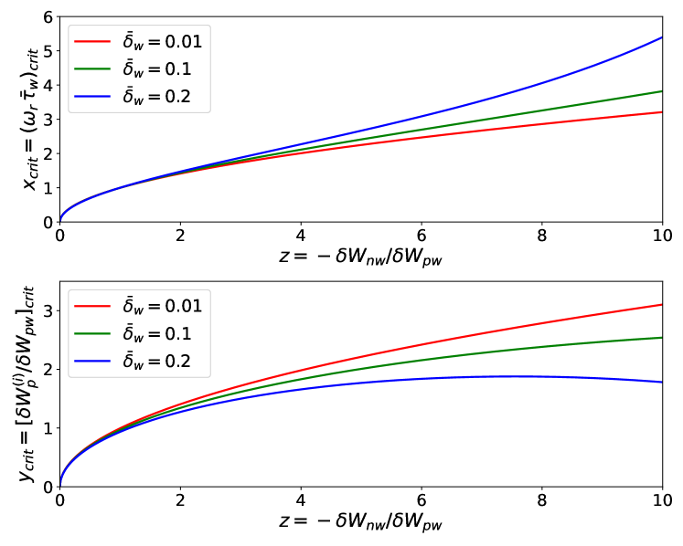
Figure 6 shows the critical real frequency, , and the critical imaginary part of the plasma potential energy, , needed to stabilize the resistive wall mode, according to the generalized Hu-Betti formula, (193). It can be seen that increasing wall thickness (at fixed ) facilitates the stabilization of the resistive wall mode, because it decreases the critical value of , which corresponds to a decreased critical plasma rotational rate. On the other hand, the real frequency of the mode at the marginal stability point increases with increasing wall thickness. Note, finally, that the thick-wall stabilization criterion only differs substantially from the thin-wall stabilization criterion, which is
| (203) |
when , which implies that the corresponding external-kink mode lies fairly close to the perfect-wall stability boundary.
V.3 Toroidal Electromagnetic Torque
As pointed out by J.-K. Park,park there is an intimate connection between the imaginary component of the plasma potential energy, , and the net toroidal electromagnetic torque exerted by the resistive wall on the plasma. Let us investigate this connection.
Employing the cylindrical analysis of Sect. IV, the net outward flux of toroidal angular momentum across a magnetic flux-surface of minor radius , lying outside the plasma, is tj
| (204) |
Given that in a vacuum region, we deduce that
| (205) |
where the additional factor of comes from averaging , and is the toroidal mode number. However, it is clear from Eq. (147) that
| (206) |
Hence, we conclude that
| (207) |
in any vacuum region.t3
Now, in the vacuum region beyond the wall,
| (208) |
[see Eq. (86)] where is the value of the perturbed poloidal magnetic flux at the plasma boundary, and
| (209) |
[See Eq. (150).] However, it is obvious from Eqs. (205) and (208) that
| (210) |
In other words, the net flux of toroidal angular momentum from the plasma-wall system is zero.
Now, in the vacuum region between the plasma and the wall,
| (211) |
[see Eq. (85)], where . [See Eq. (88).] Here,
| (212) |
[See Eq. (154).] Note that
| (213) |
It follows from Eqs. (205) and (211) that
| (214) |
Thus, if possesses an imaginary component then there is a constant flux of toroidal electromagnetic angular momentum between the plasma and the wall. This flux is associated with a toroidal electromagnetic torque exerted on the plasma, and an equal and opposite torque exerted on the wall.
Now, according to Eqs. (132), (151), (156), (162), and (163),
| (215) |
which implies that
| (216) |
Here, we have made use of the fact that and are obviously real quantities. Hence, we deduce from Eq. (214) that park
| (217) |
Here, is the toroidal electromagnetic torque acting on the plasma. It follows that the variable , appearing in the analysis of Sect. V.2, represents a normalized electromagnetic torque exerted by the wall on the plasma. In fact,
| (218) |
Thus, we can reinterpret Fig. 6 as stating, firstly, that the rotational stabilization of the resistive wall mode requires the assistance of such a torque, and, secondly, that the critical torque needed to stabilize the mode decreases with increasing wall thickness (at constant ).
VI Summary
This paper investigates the external-kink stability of a toroidal plasma surrounded by a rigid resistive wall. The main aim of this paper is to extend the well-known analysis of Haney & Freidberg hf to allow for a wall that is sufficiently thick that the thin-shell approximation does not necessarily hold. First, in Sect. III.3, we demonstrate that the MHD force operator remains self-adjoint in the presence of a thick resistive wall. Next, in Sect. III.4, making use of the self-adjoint property, we modify the variational principle of Haney & Freidberg to allow for a thick wall. Finally, in Sect. III.5, we minimize the plasma potential energy to obtain a generalized Haney-Freidberg formula, (108) and (109), for the growth-rate of the resistive wall mode that allows the wall to lie either in the thin-shell regime, the thick-shell regime, or somewhere in between. We find that thick-wall effects do not change the marginal stability point of the mode, but introduce an interesting asymmetry between growing and decaying modes. Growing modes have growth-rates that exceed those predicted by the original Haney-Freidberg formula. (Here, we are comparing walls with differing thicknesses but the same L/R time.) On the other hand, decaying modes have decay-rates that are less than those predicted by the original formula. We can even generalize the Haney-Freidberg formula to allow for walls with varying thickness and electrical conductivity. [See Eq. (116).]
We also show, during the course of our investigation, that the eigenfunctions conventionally used to calculate the no-wall and the perfect-wall plasma potential energies of ideal external-kink mode that feature in the Haney-Freidberg formula do not satisfy the pressure balance matching condition at the plasma boundary. We then explain why this is not problematic. In particular, the resistive wall mode eigenfunction is found to satisfy the pressure balance matching condition.
In Sect. IV, we perform a cylindrical calculation for a generic force-free reversed-field pinch plasma equilibrium that reveals that thick-wall effects have no noticeable effect on the growth-rates of the various resistive wall modes to which the plasma is subject, except when the mode is question lies quite close to the perfect-wall stability boundary. For such a comparatively rapidly growing mode, thick-wall effects perceptibly increase the growth-rate.
Finally, in Sect. V, we generalize the well-known Hu-Betti formula res4 for the rotational stabilization of the resistive wall mode to take thick-wall effects into account. We find that increasing wall thickness (at fixed L/R time) facilitates the rotational stabilization of the resistive wall mode, because it decreases the critical toroidal electromagnetic torque that the wall must exert on the plasma. On the other hand, the real frequency of the mode at the marginal stability point increases with increasing wall thickness.
Acknowledgements
This research was directly funded by the U.S. Department of Energy, Office of Science, Office of Fusion Energy Sciences, under contract DE-SC0021156.
Data Availability Statement
The digital data used in the figures in this paper can be obtained from the author upon reasonable request.
References
References
- (1) G. Laval, R. Pellat and J.S. Soule, Phys. Fluids 17, 815 (1974).
- (2) R.L. Dewar, R.C. Grimm, J.L. Johnson, E.A. Frieman, J.M. Greene and P.H. Rutherford, Phys. Fluids 17, 930 (1974).
- (3) F.A. Haas, Nucl. Fusion 15, 407 (1975).
- (4) J.A. Wesson, Tokamaks, 4th Ed. (Oxford University Press, Oxford UK, 2011).
- (5) R. Fitzpatrick, Tearing Mode Dynamics in Tokamak Plasmas. (IOP, Bristol UK, 2023).
- (6) D. Pfirsch and H. Tasso, Nucl. Fusion 11, 259 (1971).
- (7) J.P. Goedbloed, D. Pfirsch and H. Tasso, Nucl. Fusion 12, 649 (1972).
- (8) I.B. Bernstein, E.A. Frieman, M.D. Kruskal and R.M. Kulsrud, Proc. R. Soc. London, Ser. A 244, 17 (1958).
- (9) J.P. Freidberg, Rev. Mod. Phys. 54, 801 (1982).
- (10) J.P. Freidberg, Ideal Magnetohydrodynamics. (Plenum, New York NY, 1987).
- (11) J.P. Goedbloed and S. Poedts, Principles of Magnetohydrodynamics. (Cambridge University Press, Cambridge UK, 2004).
- (12) S.W. Haney and J.P. Freidberg, Phys. Fluids B 1, 1637 (1989).
- (13) C.G. Gimblett, Nucl. Fusion 26, 617 (1986).
- (14) R. Fitzpatrick, S.C. Guo, D.J. Den Hartog and C.C. Hegna, Phys. Plasmas 6, 3878 (1999).
- (15) B.E. Chapman, R. Fitzpatrick, D. Craig, P. Martin and G. Spizzo, Phys. Plasmas 11, 2156 (2004).
- (16) L.-J. Zheng and M.T. Kotschenreuther, Phys. Plasmas 12, 072504 (2005).
- (17) V.D. Pustovitov, Phys. Plasmas 19, 062503 (2012).
- (18) R. Fitzpatrick, Phys. Plasmas 20, 012504 (2013).
- (19) N.D. Lepikhin and V.D. Pustovitov, Phys. Plasmas 21, 042504 (2014).
- (20) R. Fitzpatrick, Phys. Plasmas 31, 042510 (2024).
- (21) J.D. Jackson, Classical Electrodynamics, 3rd Ed. (Wiley & Sons, Hoboken NJ, 1998).
- (22) W.A. Newcomb, Ann. Phys. (NY) 10, 232 (1960).
- (23) R. Fitzpatrick, Phys. Plasmas 6, 1168 (1999).
- (24) J.W. Berkery, R. Betti, Y.Q. Liu and S.A. Sabbagh, Phys. Plasmas 30, 120901 (2023).
- (25) R. Betti and J.P. Freidberg, Phys. Rev. Lett. 74, 2949 (1995).
- (26) L.J. Zheng, M. Kotschenreuther and M.S. Chu, Phys. Rev. Lett. 95, 255003 (2005).
- (27) B. Hu and R. Betti, Phys. Rev. Lett. 93, 105002 (2004).
- (28) B. Hu, R. Betti and J. Manickam, Phys. Plasmas 12, 057301 (2005).
- (29) A. Bondeson and D. Ward, Phys. Rev. Lett. 72, 2709 (1994).
- (30) J.-K. Park, Phys. Plasmas 18, 110702 (2011).
- (31) R. Fitzpatrick, Calculation of Tearing Mode Stability in an Inverse Aspect-Ratio Expanded Tokamak Plasma Equilibrium, submitted to Physics of Plasmas (2024).
- (32) R. Fitzpatrick, R.J. Hastie, T.J. Martin and C.M. Roach, Nucl. Fusion 33, 1533 (1993).