Crosscap states and duality of Ising field theory in two dimensions
Yueshui Zhang
Physics Department and Arnold Sommerfeld Center for Theoretical Physics, Ludwig-Maximilians-Universität München, 80333 Munich, Germany
Ying-Hai Wu
School of Physics and Wuhan National High Magnetic Field Center, Huazhong University of Science and Technology, Wuhan 430074, China
Lei Wang
Institute of Physics, Chinese Academy of Sciences, Beijing 100190, China
Songshan Lake Materials Laboratory, Dongguan, Guangdong 523808, China
Hong-Hao Tu
h.tu@lmu.de
Physics Department and Arnold Sommerfeld Center for Theoretical Physics, Ludwig-Maximilians-Universität München, 80333 Munich, Germany
Abstract
We propose two distinct crosscap states for the two-dimensional (2D) Ising field theory. These two crosscap states, identifying Ising spins or dual spins (domain walls) at antipodal points, are shown to be related via the Kramers-Wannier duality transformation. We derive their Majorana free field representations and extend bosonization techniques to calculate correlation functions of the 2D Ising conformal field theory (CFT) with different crosscap boundaries. We further develop a conformal perturbation theory to calculate the Klein bottle entropy as a universal scaling function [Phys. Rev. Lett. 130, 151602 (2023) ] in the 2D Ising field theory. The formalism developed in this work is applicable to many other 2D CFTs perturbed by relevant operators.
Although the two-dimensional (2D) classical Ising model was invented one century ago [1 , 2 ] , studies on this model continue to deepen our understanding of critical phenomena at the present time. In the absence of external fields, Kramers-Wannier duality [3 ] and the exact solution [4 , 5 , 6 , 7 , 8 ] reveal a second-order phase transition at a critical temperature. At this critical point, scale invariance is promoted to conformal invariance [9 , 10 , 11 ] , identifying the critical theory as the simplest conformal field theory (CFT) in two dimensions, known as the 2D Ising CFT [12 ] . In the vicinity of the critical point, the correlation length is much larger than the lattice spacing, so low-energy physics can be captured using a continuous field theory description. Considering the two relevant perturbations (thermal and magnetic perturbations, driven by temperature and external field, respectively), the scaling limit of the 2D classical Ising model is described by the 2D Ising field theory [13 , 14 ] , which has attracted considerable interest [15 , 16 , 17 , 18 , 19 , 20 ] .
There have been significant advances in the study of 2D CFTs on non-orientable manifolds [21 , 22 , 23 , 24 , 25 , 26 , 27 ] , such as the Klein bottle and the real projective plane (ℝ ℙ 2 ℝ superscript ℙ 2 \mathbb{RP}^{2} [28 , 29 , 30 , 31 ] . In general, crosscap boundary states (and the associated crosscap coefficients) are crucial information for understanding the properties of 2D CFTs on non-orientable manifolds. For the 2D Ising CFT, the crosscap coefficients and certain two-point correlation functions on the ℝ ℙ 2 ℝ superscript ℙ 2 \mathbb{RP}^{2} [32 , 33 ] .
In this Letter, we demonstrate that there are at least two distinct crosscap states for the 2D Ising field theory, both at and away from criticality. We begin with a lattice formulation (quantum Ising chain) and propose two physically motivated crosscap states on the lattice. These lattice crosscap states identify Ising spins and dual spins (domain walls) at antipodal points, respectively, and are related to each other through the Kramers-Wannier duality. Remarkably, the overlaps between the lattice crosscap states and the eigenstates of the critical Ising chain are universal (without finite-size corrections), enabling us to derive Majorana free field representations of the crosscap states in the continuum limit. In the context of the 2D Ising CFT, one of these crosscap states is already known [22 ] but the other has not been discussed in the literature to the best of our knowledge. Away from criticality, we develop a conformal perturbation theory to calculate the overlap of crosscap states with perturbed ground states, which we call crosscap overlap . This formalism is applicable to any 2D CFT perturbed by relevant operators, thus providing a systematic method to calculate the Klein bottle entropy [34 , 35 , 36 , 37 , 38 , 39 ] (norm-square of the crosscap overlap) as a universal scaling function of dimensionless coupling strengths [40 ] . For the 2D Ising field theory, the leading-order expansions of the Klein bottle entropy derived from the conformal perturbation theory are verified in lattice models by numerical simulations. Our findings open up new avenues for exploring many other 2D field theories on non-orientable manifolds.
Ising crosscap states — We start with the Hamiltonian formulation of the 2D Ising field theory [14 ]
H = H 0 − g 1 ∫ 0 L d x ε ( x ) − g 2 ∫ 0 L d x σ ( x ) , 𝐻 subscript 𝐻 0 subscript 𝑔 1 superscript subscript 0 𝐿 differential-d 𝑥 𝜀 𝑥 subscript 𝑔 2 superscript subscript 0 𝐿 differential-d 𝑥 𝜎 𝑥 \displaystyle H=H_{0}-g_{1}\int_{0}^{L}\mathrm{d}x\,\varepsilon(x)-g_{2}\int_{0}^{L}\mathrm{d}x\,\sigma(x)\,, (1)
where H 0 subscript 𝐻 0 H_{0} c = 1 / 2 𝑐 1 2 c=1/2 ε 𝜀 \varepsilon σ 𝜎 \sigma ( 1 / 2 , 1 / 2 ) 1 2 1 2 (1/2,1/2) ( 1 / 16 , 1 / 16 ) 1 16 1 16 (1/16,1/16) g 1 subscript 𝑔 1 g_{1} g 2 subscript 𝑔 2 g_{2} 1 L 𝐿 L
To reveal different crosscap states, we first focus on the critical point (g 1 = g 2 = 0 subscript 𝑔 1 subscript 𝑔 2 0 g_{1}=g_{2}=0
H latt = − ∑ j = 1 N σ j x σ j + 1 x − ∑ j = 1 N σ j z , subscript 𝐻 latt superscript subscript 𝑗 1 𝑁 subscript superscript 𝜎 𝑥 𝑗 subscript superscript 𝜎 𝑥 𝑗 1 superscript subscript 𝑗 1 𝑁 subscript superscript 𝜎 𝑧 𝑗 \displaystyle H_{\mathrm{latt}}=-\sum_{j=1}^{N}\sigma^{x}_{j}\sigma^{x}_{j+1}-\sum_{j=1}^{N}\sigma^{z}_{j}\,, (2)
where σ j α subscript superscript 𝜎 𝛼 𝑗 \sigma^{\alpha}_{j} α = x , z 𝛼 𝑥 𝑧
\alpha=x,z j 𝑗 j N 𝑁 N N 𝑁 N σ N + 1 α = σ 1 α superscript subscript 𝜎 𝑁 1 𝛼 superscript subscript 𝜎 1 𝛼 \sigma_{N+1}^{\alpha}=\sigma_{1}^{\alpha} 1 H latt ′ = ( 1 − h z ) ∑ j = 1 N σ j z − h x ∑ j = 1 N σ j x subscript superscript 𝐻 ′ latt 1 subscript ℎ 𝑧 superscript subscript 𝑗 1 𝑁 superscript subscript 𝜎 𝑗 𝑧 subscript ℎ 𝑥 superscript subscript 𝑗 1 𝑁 superscript subscript 𝜎 𝑗 𝑥 H^{\prime}_{\mathrm{latt}}=(1-h_{z})\sum_{j=1}^{N}\sigma_{j}^{z}-h_{x}\sum_{j=1}^{N}\sigma_{j}^{x} ε ( x ) 𝜀 𝑥 \varepsilon(x) σ ( x ) 𝜎 𝑥 \sigma(x) − σ j z superscript subscript 𝜎 𝑗 𝑧 -\sigma_{j}^{z} σ j x subscript superscript 𝜎 𝑥 𝑗 \sigma^{x}_{j} g 1 ∼ 1 − h z similar-to subscript 𝑔 1 1 subscript ℎ 𝑧 g_{1}\sim 1-h_{z} g 2 ∼ h x similar-to subscript 𝑔 2 subscript ℎ 𝑥 g_{2}\sim h_{x}
The Ising chain in Eq. (2 ℤ 2 subscript ℤ 2 \mathbb{Z}_{2} [ H latt , Q ] = 0 subscript 𝐻 latt 𝑄 0 [H_{\mathrm{latt}},Q]=0 Q = ∏ j = 1 N σ j z 𝑄 superscript subscript product 𝑗 1 𝑁 superscript subscript 𝜎 𝑗 𝑧 Q=\prod_{j=1}^{N}\sigma_{j}^{z} Q 𝑄 Q ℤ 2 subscript ℤ 2 \mathbb{Z}_{2} Q = 1 𝑄 1 Q=1 ℤ 2 subscript ℤ 2 \mathbb{Z}_{2} Q = − 1 𝑄 1 Q=-1 [12 ] , are called Neveu-Schwarz (NS) and Ramond (R) sectors, respectively. If we restrict ourselves to the NS sector, the critical Ising chain (2 U KW = e i π 4 N ∏ j = 1 N − 1 ( e − i π 4 σ j z e − i π 4 σ j x σ j + 1 x ) e − i π 4 σ N z subscript 𝑈 KW superscript 𝑒 𝑖 𝜋 4 𝑁 superscript subscript product 𝑗 1 𝑁 1 superscript 𝑒 𝑖 𝜋 4 superscript subscript 𝜎 𝑗 𝑧 superscript 𝑒 𝑖 𝜋 4 subscript superscript 𝜎 𝑥 𝑗 subscript superscript 𝜎 𝑥 𝑗 1 superscript 𝑒 𝑖 𝜋 4 superscript subscript 𝜎 𝑁 𝑧 U_{\mathrm{KW}}=e^{i\frac{\pi}{4}N}\prod_{j=1}^{N-1}(e^{-i\frac{\pi}{4}\sigma_{j}^{z}}e^{-i\frac{\pi}{4}\sigma^{x}_{j}\sigma^{x}_{j+1}})e^{-i\frac{\pi}{4}\sigma_{N}^{z}} [41 , 42 , 43 ] , which acts on lattice operators as U KW σ j z U KW † = σ j x σ j + 1 x subscript 𝑈 KW superscript subscript 𝜎 𝑗 𝑧 subscript superscript 𝑈 † KW superscript subscript 𝜎 𝑗 𝑥 superscript subscript 𝜎 𝑗 1 𝑥 U_{\mathrm{KW}}\sigma_{j}^{z}U^{{\dagger}}_{\mathrm{KW}}=\sigma_{j}^{x}\sigma_{j+1}^{x} U KW σ j x U KW † = σ 1 y ∏ l = 2 j σ l z subscript 𝑈 KW superscript subscript 𝜎 𝑗 𝑥 subscript superscript 𝑈 † KW superscript subscript 𝜎 1 𝑦 superscript subscript product 𝑙 2 𝑗 superscript subscript 𝜎 𝑙 𝑧 U_{\mathrm{KW}}\sigma_{j}^{x}U^{{\dagger}}_{\mathrm{KW}}=\sigma_{1}^{y}\prod_{l=2}^{j}\sigma_{l}^{z}
We propose one of the two lattice crosscap states as follows:
| 𝒞 latt + ⟩ = ∏ j = 1 N / 2 ( 1 + σ j x σ j + N / 2 x ) | ⇑ ⟩ , ket subscript superscript 𝒞 latt superscript subscript product 𝑗 1 𝑁 2 1 subscript superscript 𝜎 𝑥 𝑗 subscript superscript 𝜎 𝑥 𝑗 𝑁 2 ket ⇑ \displaystyle|\mathcal{C}^{+}_{\mathrm{latt}}\rangle=\prod_{j=1}^{N/2}(1+\sigma^{x}_{j}\sigma^{x}_{j+N/2})|\Uparrow\rangle\,, (3)
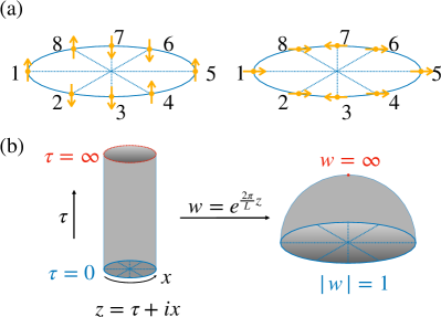
where | ⇑ ⟩ ≡ | ↑ 1 ↑ 2 ⋯ ↑ N ⟩ |\Uparrow\rangle\equiv|\uparrow_{1}\uparrow_{2}\cdots\uparrow_{N}\rangle σ z superscript 𝜎 𝑧 \sigma^{z} | 𝒞 latt + ⟩ ket subscript superscript 𝒞 latt |\mathcal{C}^{+}_{\mathrm{latt}}\rangle | ↑ ↑ ⟩ + | ↓ ↓ ⟩ |\uparrow\uparrow\rangle+|\downarrow\downarrow\rangle j 𝑗 j j + N / 2 𝑗 𝑁 2 j+N/2 [44 , 45 , 46 , 47 , 48 , 49 ] , as depicted in Fig. 1
The other crosscap state is obtained by applying the Kramers-Wannier duality transformation to | 𝒞 latt + ⟩ ket subscript superscript 𝒞 latt |\mathcal{C}^{+}_{\mathrm{latt}}\rangle
| 𝒞 latt − ⟩ ket subscript superscript 𝒞 latt \displaystyle|\mathcal{C}^{-}_{\mathrm{latt}}\rangle ≡ U KW | 𝒞 latt + ⟩ absent subscript 𝑈 KW ket subscript superscript 𝒞 latt \displaystyle\equiv U_{\mathrm{KW}}|\mathcal{C}^{+}_{\mathrm{latt}}\rangle
= ∏ j = 1 N / 2 ( 1 + μ j μ j + N / 2 ) 1 2 ( | ⇒ ⟩ + | ⇐ ⟩ ) , absent superscript subscript product 𝑗 1 𝑁 2 1 subscript 𝜇 𝑗 subscript 𝜇 𝑗 𝑁 2 1 2 ket ⇒ ket ⇐ \displaystyle=\prod_{j=1}^{N/2}\left(1+\mu_{j}\mu_{j+N/2}\right)\tfrac{1}{\sqrt{2}}(|\Rightarrow\rangle+|\Leftarrow\rangle)\,, (4)
where μ j = ∏ l = 1 j σ l z subscript 𝜇 𝑗 superscript subscript product 𝑙 1 𝑗 superscript subscript 𝜎 𝑙 𝑧 \mu_{j}=\prod_{l=1}^{j}\sigma_{l}^{z} | ⇒ ⟩ ≡ | → 1 → 2 ⋯ → N ⟩ |\Rightarrow\rangle\equiv|\rightarrow_{1}\rightarrow_{2}\cdots\rightarrow_{N}\rangle | ⇐ ⟩ ≡ | ← 1 ← 2 ⋯ ← N ⟩ |\Leftarrow\rangle\equiv|\leftarrow_{1}\leftarrow_{2}\cdots\leftarrow_{N}\rangle σ x superscript 𝜎 𝑥 \sigma^{x} | → ⟩ = 1 2 ( | ↑ ⟩ + | ↓ ⟩ ) ket → 1 2 ket ↑ ket ↓ |\rightarrow\rangle=\frac{1}{\sqrt{2}}(|\uparrow\rangle+|\downarrow\rangle) | ← ⟩ = 1 2 ( | ↑ ⟩ − | ↓ ⟩ ) ket ← 1 2 ket ↑ ket ↓ |\leftarrow\rangle=\frac{1}{\sqrt{2}}(|\uparrow\rangle-|\downarrow\rangle) σ z superscript 𝜎 𝑧 \sigma^{z} σ x superscript 𝜎 𝑥 \sigma^{x} μ j μ j + N / 2 subscript 𝜇 𝑗 subscript 𝜇 𝑗 𝑁 2 \mu_{j}\mu_{j+N/2} domain walls at antipodal positions on top of | ⇒ ⟩ ket ⇒ |\Rightarrow\rangle | ⇐ ⟩ ket ⇐ |\Leftarrow\rangle 1 | 𝒞 latt − ⟩ ket subscript superscript 𝒞 latt |\mathcal{C}^{-}_{\mathrm{latt}}\rangle dual spins (domain walls) at the antipodal sites.
Figure 1: Schematics of (a) typical configurations from lattice crosscap states | 𝒞 latt + ⟩ ket subscript superscript 𝒞 latt |\mathcal{C}^{+}_{\mathrm{latt}}\rangle | 𝒞 latt − ⟩ ket subscript superscript 𝒞 latt |\mathcal{C}^{-}_{\mathrm{latt}}\rangle ℝ ℙ 2 ℝ superscript ℙ 2 \mathbb{RP}^{2}
With the lattice crosscap state proposals in hand, our next task is to identify their field theory counterparts in the continuum limit. To this end, we adopt the strategy of computing the overlaps of | 𝒞 latt ± ⟩ ket superscript subscript 𝒞 latt plus-or-minus |\mathcal{C}_{\mathrm{latt}}^{\pm}\rangle 2
To compute the overlaps, we solve the critical Ising chain (2 [50 ] , σ j x = ( c j † + c j ) ∏ l = 1 j − 1 e i π c l † c l superscript subscript 𝜎 𝑗 𝑥 superscript subscript 𝑐 𝑗 † subscript 𝑐 𝑗 superscript subscript product 𝑙 1 𝑗 1 superscript 𝑒 𝑖 𝜋 superscript subscript 𝑐 𝑙 † subscript 𝑐 𝑙 \sigma_{j}^{x}=(c_{j}^{\dagger}+c_{j})\prod_{l=1}^{j-1}e^{i\pi c_{l}^{\dagger}c_{l}} σ j z = 2 c j † c j − 1 subscript superscript 𝜎 𝑧 𝑗 2 subscript superscript 𝑐 † 𝑗 subscript 𝑐 𝑗 1 \sigma^{z}_{j}=2c^{\dagger}_{j}c_{j}-1 Q | 𝒞 latt ± ⟩ = | 𝒞 latt ± ⟩ 𝑄 ket superscript subscript 𝒞 latt plus-or-minus ket superscript subscript 𝒞 latt plus-or-minus Q|\mathcal{C}_{\mathrm{latt}}^{\pm}\rangle=|\mathcal{C}_{\mathrm{latt}}^{\pm}\rangle 2 c j = 1 N ∑ k ∈ NS e i k j c k subscript 𝑐 𝑗 1 𝑁 subscript 𝑘 NS superscript 𝑒 𝑖 𝑘 𝑗 subscript 𝑐 𝑘 c_{j}=\frac{1}{\sqrt{N}}\sum_{k\in\mathrm{NS}}e^{ikj}c_{k}
H latt NS = ∑ k ∈ NS 4 cos k 2 ( d k † d k − 1 2 ) , subscript superscript 𝐻 NS latt subscript 𝑘 NS 4 𝑘 2 superscript subscript 𝑑 𝑘 † subscript 𝑑 𝑘 1 2 \displaystyle H^{\mathrm{NS}}_{\mathrm{latt}}=\sum_{k\in\mathrm{NS}}4\cos\frac{k}{2}\left(d_{k}^{\dagger}d_{k}-\frac{1}{2}\right), (5)
where d k = e i π / 4 sin k 4 c k + e − i π / 4 cos k 4 c − k † subscript 𝑑 𝑘 superscript 𝑒 𝑖 𝜋 4 𝑘 4 subscript 𝑐 𝑘 superscript 𝑒 𝑖 𝜋 4 𝑘 4 superscript subscript 𝑐 𝑘 † d_{k}=e^{i\pi/4}\sin\frac{k}{4}c_{k}+e^{-i\pi/4}\cos\frac{k}{4}c_{-k}^{\dagger} k ∈ NS 𝑘 NS k\in\mathrm{NS} k = ± [ π − 2 π N ( n k − 1 2 ) ] 𝑘 plus-or-minus delimited-[] 𝜋 2 𝜋 𝑁 subscript 𝑛 𝑘 1 2 k=\pm[\pi-\frac{2\pi}{N}(n_{k}-\frac{1}{2})] n k = 1 , 2 , … , N / 2 subscript 𝑛 𝑘 1 2 … 𝑁 2
n_{k}=1,2,\ldots,N/2 n k ∈ ℤ + subscript 𝑛 𝑘 superscript ℤ n_{k}\in\mathbb{Z}^{+} 5 d k subscript 𝑑 𝑘 d_{k}
| 0 ⟩ d = ∏ k > 0 ( sin k 4 + i cos k 4 c k † c − k † ) | 0 ⟩ c , subscript ket 0 𝑑 subscript product 𝑘 0 𝑘 4 𝑖 𝑘 4 superscript subscript 𝑐 𝑘 † superscript subscript 𝑐 𝑘 † subscript ket 0 𝑐 \displaystyle|0\rangle_{d}=\prod_{k>0}\left(\sin\frac{k}{4}+i\cos\frac{k}{4}c_{k}^{\dagger}c_{-k}^{\dagger}\right)|0\rangle_{c}\,, (6)
where | 0 ⟩ c subscript ket 0 𝑐 |0\rangle_{c} c j | 0 ⟩ c = 0 ∀ j subscript 𝑐 𝑗 subscript ket 0 𝑐 0 for-all 𝑗 c_{j}|0\rangle_{c}=0\;\forall j | 0 ⟩ c subscript ket 0 𝑐 |0\rangle_{c} | ⇓ ⟩ ≡ | ↓ 1 ↓ 2 ⋯ ↓ N ⟩ |\Downarrow\rangle\equiv|\downarrow_{1}\downarrow_{2}\cdots\downarrow_{N}\rangle 5 d k † subscript superscript 𝑑 † 𝑘 d^{{\dagger}}_{k} | 0 ⟩ d subscript ket 0 𝑑 |0\rangle_{d}
A key observation which enables the overlap computation is
| 𝒞 latt + ⟩ ket subscript superscript 𝒞 latt \displaystyle|\mathcal{C}^{+}_{\mathrm{latt}}\rangle = 1 − i 2 ∏ j = 1 N / 2 ( 1 + i c j † c j + N / 2 † ) | 0 ⟩ c absent 1 𝑖 2 superscript subscript product 𝑗 1 𝑁 2 1 𝑖 superscript subscript 𝑐 𝑗 † superscript subscript 𝑐 𝑗 𝑁 2 † subscript ket 0 𝑐 \displaystyle=\frac{1-i}{2}\prod_{j=1}^{N/2}(1+ic_{j}^{\dagger}c_{j+N/2}^{\dagger})|0\rangle_{c}
+ 1 + i 2 ∏ j = 1 N / 2 ( 1 − i c j † c j + N / 2 † ) | 0 ⟩ c , 1 𝑖 2 superscript subscript product 𝑗 1 𝑁 2 1 𝑖 superscript subscript 𝑐 𝑗 † superscript subscript 𝑐 𝑗 𝑁 2 † subscript ket 0 𝑐 \displaystyle\phantom{=}\;+\frac{1+i}{2}\prod_{j=1}^{N/2}(1-ic_{j}^{\dagger}c_{j+N/2}^{\dagger})|0\rangle_{c}\,, (7)
where | 𝒞 latt + ⟩ ket subscript superscript 𝒞 latt |\mathcal{C}^{+}_{\mathrm{latt}}\rangle 7 5 | ψ k 1 ⋯ k M ⟩ = ∏ α = 1 M ( i d − k α † d k α † ) | 0 ⟩ d ket subscript 𝜓 subscript 𝑘 1 ⋯ subscript 𝑘 𝑀 superscript subscript product 𝛼 1 𝑀 𝑖 superscript subscript 𝑑 subscript 𝑘 𝛼 † superscript subscript 𝑑 subscript 𝑘 𝛼 † subscript ket 0 𝑑 |\psi_{k_{1}\cdots k_{M}}\rangle=\prod_{\alpha=1}^{M}(id_{-k_{\alpha}}^{\dagger}d_{k_{\alpha}}^{\dagger})|0\rangle_{d} 0 < k 1 < ⋯ < k M < π 0 subscript 𝑘 1 ⋯ subscript 𝑘 𝑀 𝜋 0<k_{1}<\cdots<k_{M}<\pi | 𝒞 latt + ⟩ ket subscript superscript 𝒞 latt |\mathcal{C}^{+}_{\mathrm{latt}}\rangle [43 ] :
⟨ ψ k 1 ⋯ k M | 𝒞 latt + ⟩ = { ( − 1 ) ∑ α = 1 M n k α 2 + 2 2 M even i ( − 1 ) ∑ α = 1 M n k α 2 − 2 2 M odd . inner-product subscript 𝜓 subscript 𝑘 1 ⋯ subscript 𝑘 𝑀 subscript superscript 𝒞 latt cases superscript 1 superscript subscript 𝛼 1 𝑀 subscript 𝑛 subscript 𝑘 𝛼 2 2 2 𝑀 even 𝑖 superscript 1 superscript subscript 𝛼 1 𝑀 subscript 𝑛 subscript 𝑘 𝛼 2 2 2 𝑀 odd \displaystyle\langle\psi_{k_{1}\cdots k_{M}}|\mathcal{C}^{+}_{\mathrm{latt}}\rangle=\begin{cases}(-1)^{\sum_{\alpha=1}^{M}n_{k_{\alpha}}}\sqrt{\frac{2+\sqrt{2}}{2}}&M\;\mathrm{even}\\
i(-1)^{\sum_{\alpha=1}^{M}n_{k_{\alpha}}}\sqrt{\frac{2-\sqrt{2}}{2}}&M\;\mathrm{odd}\\
\end{cases}\,. (8)
Most remarkably, the overlaps in Eq. (8 N ≥ 4 𝑁 4 N\geq 4
For the other lattice crosscap state | 𝒞 latt − ⟩ ket subscript superscript 𝒞 latt |\mathcal{C}^{-}_{\mathrm{latt}}\rangle 5 U KW d k † U KW † = i e − i k / 2 d k † subscript 𝑈 KW superscript subscript 𝑑 𝑘 † superscript subscript 𝑈 KW † 𝑖 superscript 𝑒 𝑖 𝑘 2 superscript subscript 𝑑 𝑘 † U_{\mathrm{KW}}d_{k}^{\dagger}U_{\mathrm{KW}}^{\dagger}=ie^{-ik/2}d_{k}^{\dagger} U KW | 0 ⟩ d = | 0 ⟩ d subscript 𝑈 KW subscript ket 0 𝑑 subscript ket 0 𝑑 U_{\mathrm{KW}}|0\rangle_{d}=|0\rangle_{d} [43 ] , we obtain ⟨ ψ k 1 ⋯ k M | 𝒞 latt − ⟩ = ( − 1 ) M ⟨ ψ k 1 ⋯ k M | 𝒞 latt + ⟩ inner-product subscript 𝜓 subscript 𝑘 1 ⋯ subscript 𝑘 𝑀 subscript superscript 𝒞 latt superscript 1 𝑀 inner-product subscript 𝜓 subscript 𝑘 1 ⋯ subscript 𝑘 𝑀 subscript superscript 𝒞 latt \langle\psi_{k_{1}\cdots k_{M}}|\mathcal{C}^{-}_{\mathrm{latt}}\rangle=(-1)^{M}\langle\psi_{k_{1}\cdots k_{M}}|\mathcal{C}^{+}_{\mathrm{latt}}\rangle
In the continuum limit, the low-energy effective Hamiltonian for the lattice model (5 [12 ]
H 0 NS = 2 π L [ ∑ n = 1 ∞ ( n − 1 2 ) ( b n − 1 2 † b n − 1 2 + b ¯ n − 1 2 † b ¯ n − 1 2 ) − c 12 ] subscript superscript 𝐻 NS 0 2 𝜋 𝐿 delimited-[] superscript subscript 𝑛 1 𝑛 1 2 subscript superscript 𝑏 † 𝑛 1 2 subscript 𝑏 𝑛 1 2 subscript superscript ¯ 𝑏 † 𝑛 1 2 subscript ¯ 𝑏 𝑛 1 2 𝑐 12 \displaystyle H^{\mathrm{NS}}_{0}=\frac{2\pi}{L}\left[\sum_{n=1}^{\infty}(n-\frac{1}{2})\left(b^{{\dagger}}_{n-\frac{1}{2}}b_{n-\frac{1}{2}}+\bar{b}^{{\dagger}}_{n-\frac{1}{2}}\bar{b}_{n-\frac{1}{2}}\right)-\frac{c}{12}\right] (9)
with b n − 1 2 † subscript superscript 𝑏 † 𝑛 1 2 b^{{\dagger}}_{n-\frac{1}{2}} b n − 1 2 subscript 𝑏 𝑛 1 2 b_{n-\frac{1}{2}} 9 5 ( d k , d k † ) ⇔ ( b n k − 1 2 , b n k − 1 2 † ) ⇔ subscript 𝑑 𝑘 superscript subscript 𝑑 𝑘 † subscript 𝑏 subscript 𝑛 𝑘 1 2 subscript superscript 𝑏 † subscript 𝑛 𝑘 1 2 (d_{k},d_{k}^{\dagger})\Leftrightarrow(b_{n_{k}-\frac{1}{2}},b^{{\dagger}}_{n_{k}-\frac{1}{2}}) ( i d − k , − i d − k † ) ⇔ ( b ¯ n k − 1 2 , b ¯ n k − 1 2 † ) ⇔ 𝑖 subscript 𝑑 𝑘 𝑖 superscript subscript 𝑑 𝑘 † subscript ¯ 𝑏 subscript 𝑛 𝑘 1 2 subscript superscript ¯ 𝑏 † subscript 𝑛 𝑘 1 2 (id_{-k},-id_{-k}^{\dagger})\Leftrightarrow(\bar{b}_{n_{k}-\frac{1}{2}},\bar{b}^{{\dagger}}_{n_{k}-\frac{1}{2}}) k 𝑘 k ± π plus-or-minus 𝜋 \pm\pi 5 9 U KW b n − 1 2 U KW † = b n − 1 2 subscript 𝑈 KW subscript 𝑏 𝑛 1 2 subscript superscript 𝑈 † KW subscript 𝑏 𝑛 1 2 U_{\mathrm{KW}}b_{n-\frac{1}{2}}U^{{\dagger}}_{\mathrm{KW}}=b_{n-\frac{1}{2}} U KW b ¯ n − 1 2 U KW † = − b ¯ n − 1 2 subscript 𝑈 KW subscript ¯ 𝑏 𝑛 1 2 subscript superscript 𝑈 † KW subscript ¯ 𝑏 𝑛 1 2 U_{\mathrm{KW}}\bar{b}_{n-\frac{1}{2}}U^{{\dagger}}_{\mathrm{KW}}=-\bar{b}_{n-\frac{1}{2}}
In the continuum limit, the eigenstates | ψ k 1 ⋯ k M ⟩ ket subscript 𝜓 subscript 𝑘 1 ⋯ subscript 𝑘 𝑀 |\psi_{k_{1}\cdots k_{M}}\rangle 8 ∏ α = 1 M b n k α − 1 2 † b ¯ n k α − 1 2 † | 0 ⟩ NS superscript subscript product 𝛼 1 𝑀 subscript superscript 𝑏 † subscript 𝑛 subscript 𝑘 𝛼 1 2 subscript superscript ¯ 𝑏 † subscript 𝑛 subscript 𝑘 𝛼 1 2 subscript ket 0 NS \prod_{\alpha=1}^{M}b^{{\dagger}}_{n_{k_{\alpha}}-\frac{1}{2}}\bar{b}^{{\dagger}}_{n_{k_{\alpha}}-\frac{1}{2}}|0\rangle_{\mathrm{NS}} | 0 ⟩ NS subscript ket 0 NS |0\rangle_{\mathrm{NS}} 8
| 𝒞 ± ⟩ ket subscript 𝒞 plus-or-minus \displaystyle|\mathcal{C}_{\pm}\rangle = e i π / 8 2 exp [ ± ∑ n = 1 ∞ ( − 1 ) n b n − 1 2 † b ¯ n − 1 2 † ] | 0 ⟩ NS absent superscript 𝑒 𝑖 𝜋 8 2 plus-or-minus superscript subscript 𝑛 1 superscript 1 𝑛 subscript superscript 𝑏 † 𝑛 1 2 subscript superscript ¯ 𝑏 † 𝑛 1 2 subscript ket 0 NS \displaystyle=\frac{e^{i\pi/8}}{\sqrt{2}}\exp\left[\pm\sum_{n=1}^{\infty}(-1)^{n}b^{{\dagger}}_{n-\frac{1}{2}}\bar{b}^{{\dagger}}_{n-\frac{1}{2}}\right]|0\rangle_{\mathrm{NS}}
+ e − i π / 8 2 exp [ ∓ ∑ n = 1 ∞ ( − 1 ) n b n − 1 2 † b ¯ n − 1 2 † ] | 0 ⟩ NS . superscript 𝑒 𝑖 𝜋 8 2 minus-or-plus superscript subscript 𝑛 1 superscript 1 𝑛 subscript superscript 𝑏 † 𝑛 1 2 subscript superscript ¯ 𝑏 † 𝑛 1 2 subscript ket 0 NS \displaystyle\phantom{=}+\frac{e^{-i\pi/8}}{\sqrt{2}}\exp\left[\mp\sum_{n=1}^{\infty}(-1)^{n}b^{{\dagger}}_{n-\frac{1}{2}}\bar{b}^{{\dagger}}_{n-\frac{1}{2}}\right]|0\rangle_{\mathrm{NS}}\,. (10)
The crosscap Ishibashi states of the 2D Ising CFT are labeled by the primary fields as | a ⟩ ⟩ 𝒞 |a\rangle\rangle_{\mathcal{C}} a = 𝟙 , σ , ε 𝑎 1 𝜎 𝜀
a=\mathbbm{1},\sigma,\varepsilon [21 , 22 ] . The crosscap states | 𝒞 ± ⟩ ket subscript 𝒞 plus-or-minus |\mathcal{C}_{\pm}\rangle 10
| 𝒞 ± ⟩ = 2 + 2 2 | 𝟙 ⟩ ⟩ 𝒞 ± 2 − 2 2 | ε ⟩ ⟩ 𝒞 , \displaystyle|\mathcal{C}_{\pm}\rangle=\sqrt{\frac{2+\sqrt{2}}{2}}|\mathbbm{1}\rangle\rangle_{\mathcal{C}}\pm\sqrt{\frac{2-\sqrt{2}}{2}}|\varepsilon\rangle\rangle_{\mathcal{C}}\,, (11)
where | 𝒞 + ⟩ ket subscript 𝒞 |\mathcal{C}_{+}\rangle [22 ] while | 𝒞 − ⟩ ket subscript 𝒞 |\mathcal{C}_{-}\rangle | 𝟙 ⟩ ⟩ 𝒞 ↔ | 𝟙 ⟩ ⟩ 𝒞 |\mathbbm{1}\rangle\rangle_{\mathcal{C}}\leftrightarrow|\mathbbm{1}\rangle\rangle_{\mathcal{C}} | ε ⟩ ⟩ 𝒞 ↔ − | ε ⟩ ⟩ 𝒞 |\varepsilon\rangle\rangle_{\mathcal{C}}\leftrightarrow-|\varepsilon\rangle\rangle_{\mathcal{C}} 3 4 10 11
Crosscap correlators — The two crosscap states | 𝒞 ± ⟩ ket subscript 𝒞 plus-or-minus |\mathcal{C}_{\pm}\rangle ⟨ 𝒞 + | e − β H 0 | 𝒞 + ⟩ = ⟨ 𝒞 − | e − β H 0 | 𝒞 − ⟩ quantum-operator-product subscript 𝒞 superscript 𝑒 𝛽 subscript 𝐻 0 subscript 𝒞 quantum-operator-product subscript 𝒞 superscript 𝑒 𝛽 subscript 𝐻 0 subscript 𝒞 \langle\mathcal{C}_{+}|e^{-\beta H_{0}}|\mathcal{C}_{+}\rangle=\langle\mathcal{C}_{-}|e^{-\beta H_{0}}|\mathcal{C}_{-}\rangle z = τ + i x 𝑧 𝜏 𝑖 𝑥 z=\tau+ix τ ∈ [ 0 , ∞ ) 𝜏 0 \tau\in[0,\infty) x ∈ [ 0 , L ) 𝑥 0 𝐿 x\in[0,L) w = e 2 π z L 𝑤 superscript 𝑒 2 𝜋 𝑧 𝐿 w=e^{\frac{2\pi z}{L}} ℝ ℙ 2 ℝ superscript ℙ 2 \mathbb{RP}^{2} 1
We extend bosonization techniques [52 , 12 ] to the Ising CFT with crosscap boundaries. In this approach, the Ising crosscap correlators can be expressed in terms of those of the ℤ 2 subscript ℤ 2 \mathbb{Z}_{2}
⟨ 0 | σ ( w 1 , w ¯ 1 ) σ ( w 2 , w ¯ 2 ) | 𝒞 ± ⟩ NS = 2 + 2 2 G ± ( η ) | w 1 − w 2 | 1 4 \displaystyle{}_{\mathrm{NS}}\langle 0|\sigma(w_{1},\bar{w}_{1})\sigma(w_{2},\bar{w}_{2})|\mathcal{C}_{\pm}\rangle=\sqrt{\frac{2+\sqrt{2}}{2}}\frac{G_{\pm}(\eta)}{|w_{1}-w_{2}|^{\frac{1}{4}}} (12)
with
G ± ( η ) = 2 2 1 + 1 − η ± 2 − 2 2 1 − 1 − η ( 1 − η ) 1 8 , subscript 𝐺 plus-or-minus 𝜂 plus-or-minus 2 2 1 1 𝜂 2 2 2 1 1 𝜂 superscript 1 𝜂 1 8 \displaystyle G_{\pm}(\eta)=\frac{\frac{\sqrt{2}}{2}\sqrt{1+\sqrt{1-\eta}}\pm\frac{2-\sqrt{2}}{2}\sqrt{1-\sqrt{1-\eta}}}{(1-\eta)^{\frac{1}{8}}}\,, (13)
where w 1 subscript 𝑤 1 w_{1} w 2 subscript 𝑤 2 w_{2} ℝ ℙ 2 ℝ superscript ℙ 2 \mathbb{RP}^{2} η = | w 1 − w 2 | 2 ( 1 + | w 1 | 2 ) ( 1 + | w 2 | 2 ) 𝜂 superscript subscript 𝑤 1 subscript 𝑤 2 2 1 superscript subscript 𝑤 1 2 1 superscript subscript 𝑤 2 2 \eta=\frac{|w_{1}-w_{2}|^{2}}{(1+|w_{1}|^{2})(1+|w_{2}|^{2})} | 𝒞 + ⟩ ket subscript 𝒞 |\mathcal{C}_{+}\rangle [22 ] and the conformal partial wave decomposition [32 , 33 ] . Within the bosonization framework, we also obtain multi-point crosscap correlators for the 2D Ising CFT (see Ref. [43 ] ).
Certain crosscap correlators with two different crosscap states | 𝒞 ± ⟩ ket subscript 𝒞 plus-or-minus |\mathcal{C}_{\pm}\rangle U KW subscript 𝑈 KW U_{\mathrm{KW}} ε ↔ − ε ↔ 𝜀 𝜀 \varepsilon\leftrightarrow-\varepsilon σ ↔ μ ↔ 𝜎 𝜇 \sigma\leftrightarrow\mu μ 𝜇 \mu U KW | 0 ⟩ NS = | 0 ⟩ NS subscript 𝑈 KW subscript ket 0 NS subscript ket 0 NS U_{\mathrm{KW}}|0\rangle_{\mathrm{NS}}=|0\rangle_{\mathrm{NS}} ⟨ 0 | σ ( w 1 , w ¯ 1 ) σ ( w 2 , w ¯ 2 ) | 𝒞 ± ⟩ NS = ⟨ 0 | μ ( w 1 , w ¯ 1 ) μ ( w 2 , w ¯ 2 ) | 𝒞 ∓ ⟩ NS {}_{\mathrm{NS}}\langle 0|\sigma(w_{1},\bar{w}_{1})\sigma(w_{2},\bar{w}_{2})|\mathcal{C}_{\pm}\rangle={}_{\mathrm{NS}}\langle 0|\mu(w_{1},\bar{w}_{1})\mu(w_{2},\bar{w}_{2})|\mathcal{C}_{\mp}\rangle 12 ⟨ 0 | σ ( w 1 , w ¯ 1 ) σ ( w 2 , w ¯ 2 ) | 𝒞 ± ⟩ NS ≠ ⟨ 0 | μ ( w 1 , w ¯ 1 ) μ ( w 2 , w ¯ 2 ) | 𝒞 ± ⟩ NS {}_{\mathrm{NS}}\langle 0|\sigma(w_{1},\bar{w}_{1})\sigma(w_{2},\bar{w}_{2})|\mathcal{C}_{\pm}\rangle\neq{}_{\mathrm{NS}}\langle 0|\mu(w_{1},\bar{w}_{1})\mu(w_{2},\bar{w}_{2})|\mathcal{C}_{\pm}\rangle ℝ ℙ 2 ℝ superscript ℙ 2 \mathbb{RP}^{2}
Universal scaling functions — Although expanded in the Ising CFT basis, the validity of Ising crosscap states in Eq. (10 [40 ] . Despite the great potential of this universal scaling function (e.g., identifying critical theoreis in numerics [53 ] ), there was no systematic method to compute it analytically. We now take the first step and put forward a conformal perturbation theory below for computing the crosscap overlap expanded as coupling constants, which is applicable to general 2D CFTs with relevant perturbations.
We consider the Hamiltonian H = H 0 + H 1 𝐻 subscript 𝐻 0 subscript 𝐻 1 H=H_{0}+H_{1} H 0 subscript 𝐻 0 H_{0} L 𝐿 L H 1 = − g ∫ 0 L d x φ ( x ) subscript 𝐻 1 𝑔 superscript subscript 0 𝐿 differential-d 𝑥 𝜑 𝑥 H_{1}=-g\int_{0}^{L}\mathrm{d}x\,\varphi(x) φ 𝜑 \varphi ( h , h ¯ ) ℎ ¯ ℎ (h,\bar{h}) h = h ¯ ℎ ¯ ℎ h=\bar{h} h < 1 ℎ 1 h<1 lim x → ∞ lim L → ∞ x 4 h ⟨ φ ( 0 ) φ ( x ) ⟩ = 1 subscript → 𝑥 subscript → 𝐿 superscript 𝑥 4 ℎ delimited-⟨⟩ 𝜑 0 𝜑 𝑥 1 \lim_{x\rightarrow\infty}\lim_{L\rightarrow\infty}x^{4h}\langle\varphi(0)\varphi(x)\rangle=1 | ψ 0 ( s ) ⟩ ket subscript 𝜓 0 𝑠 |\psi_{0}(s)\rangle s = g L 2 − 2 h 𝑠 𝑔 superscript 𝐿 2 2 ℎ s=gL^{2-2h} [54 ] . Denoting the crosscap state as | 𝒞 ⟩ ket 𝒞 |\mathcal{C}\rangle ⟨ ψ 0 ( s ) | 𝒞 ⟩ inner-product subscript 𝜓 0 𝑠 𝒞 \langle\psi_{0}(s)|\mathcal{C}\rangle s 𝑠 s [40 ] .
To perform a perturbative analysis, we factorize the crosscap overlap into two parts:
⟨ ψ 0 ( s ) | 𝒞 ⟩ = Z ( s ) exp [ 1 2 W ( s ) ] inner-product subscript 𝜓 0 𝑠 𝒞 𝑍 𝑠 1 2 𝑊 𝑠 \displaystyle\langle\psi_{0}(s)|\mathcal{C}\rangle=Z(s)\,\exp\left[\frac{1}{2}W(s)\right] (14)
with Z ( s ) = ⟨ ψ 0 ( s ) | 𝒞 ⟩ / ⟨ ψ 0 ( s ) | ψ 0 ( 0 ) ⟩ 𝑍 𝑠 inner-product subscript 𝜓 0 𝑠 𝒞 inner-product subscript 𝜓 0 𝑠 subscript 𝜓 0 0 Z(s)=\langle\psi_{0}(s)|\mathcal{C}\rangle/\langle\psi_{0}(s)|\psi_{0}(0)\rangle exp [ 1 2 W ( s ) ] = ⟨ ψ 0 ( s ) | ψ 0 ( 0 ) ⟩ 1 2 𝑊 𝑠 inner-product subscript 𝜓 0 𝑠 subscript 𝜓 0 0 \exp[\frac{1}{2}W(s)]=\langle\psi_{0}(s)|\psi_{0}(0)\rangle Z ( s ) 𝑍 𝑠 Z(s) W ( s ) 𝑊 𝑠 W(s)
Z ( s ) 𝑍 𝑠 \displaystyle Z(s) = lim β → ∞ ⟨ ψ 0 ( 0 ) | 𝒯 e − ∫ 0 β d τ H 1 ( τ ) | 𝒞 ⟩ ⟨ ψ 0 ( 0 ) | 𝒯 e − ∫ 0 β d τ H 1 ( τ ) | ψ 0 ( 0 ) ⟩ , absent subscript → 𝛽 quantum-operator-product subscript 𝜓 0 0 𝒯 superscript 𝑒 superscript subscript 0 𝛽 differential-d 𝜏 subscript 𝐻 1 𝜏 𝒞 quantum-operator-product subscript 𝜓 0 0 𝒯 superscript 𝑒 superscript subscript 0 𝛽 differential-d 𝜏 subscript 𝐻 1 𝜏 subscript 𝜓 0 0 \displaystyle=\lim_{\beta\to\infty}\frac{\langle\psi_{0}(0)|\mathcal{T}e^{-\int_{0}^{\beta}\mathrm{d}\tau\,H_{1}(\tau)}|\mathcal{C}\rangle}{\langle\psi_{0}(0)|\mathcal{T}e^{-\int_{0}^{\beta}\mathrm{d}\tau\,H_{1}(\tau)}|\psi_{0}(0)\rangle}\,,
W ( s ) 𝑊 𝑠 \displaystyle W(s) = lim β → ∞ [ ⟨ 𝒯 e − ∫ 0 β d τ H 1 ( τ ) ⟩ c − π β 6 L δ c ( s ) ] , absent subscript → 𝛽 delimited-[] subscript delimited-⟨⟩ 𝒯 superscript 𝑒 superscript subscript 0 𝛽 differential-d 𝜏 subscript 𝐻 1 𝜏 c 𝜋 𝛽 6 𝐿 𝛿 𝑐 𝑠 \displaystyle=\lim_{\beta\to\infty}\left[\left\langle\mathcal{T}e^{-\int_{0}^{\beta}\mathrm{d}\tau\,H_{1}(\tau)}\right\rangle_{\mathrm{c}}-\frac{\pi\beta}{6L}\delta c(s)\right]\,, (15)
where 𝒯 𝒯 \mathcal{T} H 1 ( τ ) subscript 𝐻 1 𝜏 H_{1}(\tau) ⟨ 𝒯 e − ∫ 0 β d τ H 1 ( τ ) ⟩ c subscript delimited-⟨⟩ 𝒯 superscript 𝑒 superscript subscript 0 𝛽 differential-d 𝜏 subscript 𝐻 1 𝜏 c \langle\mathcal{T}e^{-\int_{0}^{\beta}\mathrm{d}\tau\,H_{1}(\tau)}\rangle_{\mathrm{c}} connected contribution of ⟨ ψ 0 ( 0 ) | 𝒯 e − ∫ 0 β d τ H 1 ( τ ) | ψ 0 ( 0 ) ⟩ quantum-operator-product subscript 𝜓 0 0 𝒯 superscript 𝑒 superscript subscript 0 𝛽 differential-d 𝜏 subscript 𝐻 1 𝜏 subscript 𝜓 0 0 \langle\psi_{0}(0)|\mathcal{T}e^{-\int_{0}^{\beta}\mathrm{d}\tau\,H_{1}(\tau)}|\psi_{0}(0)\rangle δ c ( s ) = lim β → ∞ 6 L π β ⟨ 𝒯 e − ∫ 0 β d τ H 1 ( τ ) ⟩ c 𝛿 𝑐 𝑠 subscript → 𝛽 6 𝐿 𝜋 𝛽 subscript delimited-⟨⟩ 𝒯 superscript 𝑒 superscript subscript 0 𝛽 differential-d 𝜏 subscript 𝐻 1 𝜏 c \delta c(s)=\lim_{\beta\to\infty}\frac{6L}{\pi\beta}\langle\mathcal{T}e^{-\int_{0}^{\beta}\mathrm{d}\tau\,H_{1}(\tau)}\rangle_{\mathrm{c}} c ( s ) ≡ δ c ( s ) + c 𝑐 𝑠 𝛿 𝑐 𝑠 𝑐 c(s)\equiv\delta c(s)+c ℝ ℙ 2 ℝ superscript ℙ 2 \mathbb{RP}^{2} 𝒯 e − ∫ 0 β d τ H 1 ( τ ) 𝒯 superscript 𝑒 superscript subscript 0 𝛽 differential-d 𝜏 subscript 𝐻 1 𝜏 \mathcal{T}e^{-\int_{0}^{\beta}\mathrm{d}\tau\,H_{1}(\tau)} g 𝑔 g rational CFTs with relevant perturbations, we have obtained a general result for the first-order correction (if nonvanishing) to the crosscap overlap [43 ] .
The perturbation strategy outlined above is certainly applicable to the Ising field theory. Below we first discuss the crosscap overlaps with | 𝒞 + ⟩ ket subscript 𝒞 |\mathcal{C}_{+}\rangle | 𝒞 − ⟩ ket subscript 𝒞 |\mathcal{C}_{-}\rangle
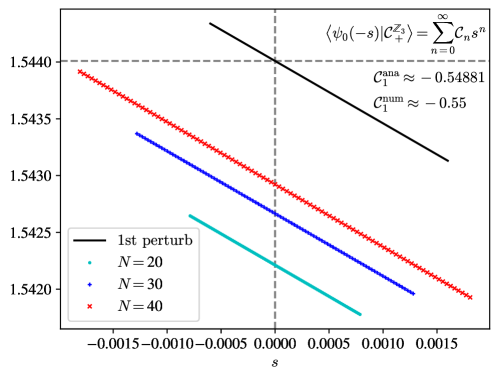
(i) For the thermal perturbation [g 1 ≠ 0 subscript 𝑔 1 0 g_{1}\neq 0 g 2 = 0 subscript 𝑔 2 0 g_{2}=0 1 ⟨ ψ 0 ( s 1 ) | 𝒞 + ⟩ inner-product subscript 𝜓 0 subscript 𝑠 1 subscript 𝒞 \langle\psi_{0}(s_{1})|\mathcal{C}_{+}\rangle s 1 = g 1 L subscript 𝑠 1 subscript 𝑔 1 𝐿 s_{1}=g_{1}L [40 ] . Our perturbative expansion agrees with the non-perturbative result order by order [43 ] .
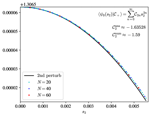
(ii) For the magnetic perturbation [g 1 = 0 subscript 𝑔 1 0 g_{1}=0 g 2 ≠ 0 subscript 𝑔 2 0 g_{2}\neq 0 1 ⟨ ψ 0 ( s 2 ) | 𝒞 + ⟩ = ∑ n = 0 ∞ 𝒞 2 n s 2 2 n inner-product subscript 𝜓 0 subscript 𝑠 2 subscript 𝒞 superscript subscript 𝑛 0 subscript 𝒞 2 𝑛 superscript subscript 𝑠 2 2 𝑛 \langle\psi_{0}(s_{2})|\mathcal{C}_{+}\rangle=\sum_{n=0}^{\infty}\mathcal{C}_{2n}s_{2}^{2n} s 2 = g 2 L 15 / 8 subscript 𝑠 2 subscript 𝑔 2 superscript 𝐿 15 8 s_{2}=g_{2}L^{15/8} σ 𝜎 \sigma 12 𝒞 2 ≈ − 1.63528 subscript 𝒞 2 1.63528 \mathcal{C}_{2}\approx-1.63528 𝒞 2 ≈ − 1.59 subscript 𝒞 2 1.59 \mathcal{C}_{2}\approx-1.59 [43 ] .
The dual crosscap overlap ⟨ ψ 0 ( s α ) | 𝒞 − ⟩ inner-product subscript 𝜓 0 subscript 𝑠 𝛼 subscript 𝒞 \langle\psi_{0}(s_{\alpha})|\mathcal{C}_{-}\rangle ⟨ ψ 0 ( s α ) | 𝒞 + ⟩ inner-product subscript 𝜓 0 subscript 𝑠 𝛼 subscript 𝒞 \langle\psi_{0}(s_{\alpha})|\mathcal{C}_{+}\rangle α = 1 , 2 𝛼 1 2
\alpha=1,2 ⟨ ψ 0 ( s α ) | 𝒞 − ⟩ = ⟨ ψ ~ 0 ( s α ) | 𝒞 + ⟩ inner-product subscript 𝜓 0 subscript 𝑠 𝛼 subscript 𝒞 inner-product subscript ~ 𝜓 0 subscript 𝑠 𝛼 subscript 𝒞 \langle\psi_{0}(s_{\alpha})|\mathcal{C}_{-}\rangle=\langle\tilde{\psi}_{0}(s_{\alpha})|\mathcal{C}_{+}\rangle | ψ ~ 0 ( s α ) ⟩ ≡ U KW | ψ 0 ( s α ) ⟩ ket subscript ~ 𝜓 0 subscript 𝑠 𝛼 subscript 𝑈 KW ket subscript 𝜓 0 subscript 𝑠 𝛼 |\tilde{\psi}_{0}(s_{\alpha})\rangle\equiv U_{\mathrm{KW}}|\psi_{0}(s_{\alpha})\rangle dual operator. For the thermal perturbation, ε ↔ − ε ↔ 𝜀 𝜀 \varepsilon\leftrightarrow-\varepsilon ⟨ ψ 0 ( s 1 ) | 𝒞 − ⟩ = ⟨ ψ 0 ( − s 1 ) | 𝒞 + ⟩ inner-product subscript 𝜓 0 subscript 𝑠 1 subscript 𝒞 inner-product subscript 𝜓 0 subscript 𝑠 1 subscript 𝒞 \langle\psi_{0}(s_{1})|\mathcal{C}_{-}\rangle=\langle\psi_{0}(-s_{1})|\mathcal{C}_{+}\rangle ⟨ ψ 0 ( s 2 ) | 𝒞 − ⟩ inner-product subscript 𝜓 0 subscript 𝑠 2 subscript 𝒞 \langle\psi_{0}(s_{2})|\mathcal{C}_{-}\rangle ⟨ ψ 0 ( s 2 ) | 𝒞 + ⟩ inner-product subscript 𝜓 0 subscript 𝑠 2 subscript 𝒞 \langle\psi_{0}(s_{2})|\mathcal{C}_{+}\rangle σ 𝜎 \sigma μ 𝜇 \mu
The overlap of the crosscap states | 𝒞 ± ⟩ ket subscript 𝒞 plus-or-minus |\mathcal{C}_{\pm}\rangle excited states should be a universal scaling function, too. Specifically, for perturbed states that are deformed from primary states, e.g., | σ , σ ¯ ⟩ ket 𝜎 ¯ 𝜎
|\sigma,\bar{\sigma}\rangle | ε , ε ¯ ⟩ ket 𝜀 ¯ 𝜀
|\varepsilon,\bar{\varepsilon}\rangle 15 τ = ∞ 𝜏 \tau=\infty [55 ] . A concrete example confirming that excited-state crosscap overlaps are also universal scaling functions is the 2D Ising CFT with thermal perturbation. As the thermal perturbation takes a quadratic form in the fermionic representation, we find the following universal overlaps between | 𝒞 ± ⟩ ket subscript 𝒞 plus-or-minus |\mathcal{C}_{\pm}\rangle 10 perturbed eigenstates [43 ] :
| ⟨ ψ n 1 ⋯ n M ( s 1 ) | 𝒞 ± ⟩ | 2 = 1 + ( − 1 ) M 1 + e ∓ 2 π s 1 , superscript inner-product subscript 𝜓 subscript 𝑛 1 ⋯ subscript 𝑛 𝑀 subscript 𝑠 1 subscript 𝒞 plus-or-minus 2 1 superscript 1 𝑀 1 superscript 𝑒 minus-or-plus 2 𝜋 subscript 𝑠 1 \displaystyle|\langle\psi_{n_{1}\cdots n_{M}}(s_{1})|\mathcal{C}_{\pm}\rangle|^{2}=1+\frac{(-1)^{M}}{\sqrt{1+e^{\mp 2\pi s_{1}}}}\,, (16)
where | ψ n 1 ⋯ n M ( s 1 ) ⟩ ket subscript 𝜓 subscript 𝑛 1 ⋯ subscript 𝑛 𝑀 subscript 𝑠 1 |\psi_{n_{1}\cdots n_{M}}(s_{1})\rangle | ψ n 1 ⋯ n M ( 0 ) ⟩ ≡ ∏ α = 1 M b n α − 1 / 2 † b ¯ n α − 1 / 2 † | 0 ⟩ NS ket subscript 𝜓 subscript 𝑛 1 ⋯ subscript 𝑛 𝑀 0 superscript subscript product 𝛼 1 𝑀 subscript superscript 𝑏 † subscript 𝑛 𝛼 1 2 subscript superscript ¯ 𝑏 † subscript 𝑛 𝛼 1 2 subscript ket 0 NS |\psi_{n_{1}\cdots n_{M}}(0)\rangle\equiv\prod_{\alpha=1}^{M}b^{\dagger}_{n_{\alpha}-1/2}\bar{b}^{\dagger}_{n_{\alpha}-1/2}|0\rangle_{\mathrm{NS}}
Summary and outlook — In conclusion, two distinct crosscap states in the 2D Ising field theory that are connected to each other via the Kramers-Wannier duality have been thoroughly investigated. The Majorana free field representation of these crosscap states are established and the bosonization approach is extended to calculate the crosscap correlators, i.e., correlation functions on the real projective plane (ℝ ℙ 2 ℝ superscript ℙ 2 \mathbb{RP}^{2} [56 ] ).
Apart from the 2D Ising field theory, duality has also been uncovered in many other field theories (e.g., ℤ N subscript ℤ 𝑁 \mathbb{Z}_{N} [57 ] ). It would be interesting to explore new crosscap states enriched by duality. This may shed light on a conjectured link between the Klein bottle entropy and the renormalization group flow [40 ] , in analogous to the c 𝑐 c [58 ] for central charge and the g 𝑔 g [59 , 60 ] for Affleck-Ludwig boundary entropy. Moreover, crosscap overlaps on lattices provide a promising route for extracting crosscap coefficients of 3D CFTs, which would complement the bootstrap approach where only ratios of crosscap coefficients were obtained [32 ] .
Acknowledgments — We are grateful to Meng Cheng, Davide Fioravanti, Anton Hulsch, Dong-Hee Kim, Jicheol Kim, Shota Komatsu, Wei Tang, and Hua-Chen Zhang for stimulating discussions. H.-H.T. extends his gratitude to Thomas Quella for many inspiring discussions and hospitality during a research visit to School of Mathematics and Statistics at the University of Melbourne, where this work is completed. Y.S.Z. is supported by the Sino-German (CSC-DAAD) Postdoc Scholarship Program. Y.H.W. is supported by the National Natural Science Foundation of China under Grant No. 12174130. L.W. is supported by National Natural Science Foundation of China under Grant No. T2225018.
References
Ising [1925]
E. Ising, Z. Phys. 31 , 253 (1925) .
McCoy and Wu [1973]
B. M. McCoy and T. T. Wu, The Two-Dimensional Ising Model
Kramers and Wannier [1941]
H. A. Kramers and G. H. Wannier, Phys. Rev. 60 , 252 (1941) .
Onsager [1944]
L. Onsager, Phys. Rev. 65 , 117 (1944) .
Kaufman [1949]
B. Kaufman, Phys. Rev. 76 , 1232 (1949) .
Kaufman and Onsager [1949]
B. Kaufman and L. Onsager, Phys. Rev. 76 , 1244 (1949) .
Yang [1952]
C. N. Yang, Phys. Rev. 85 , 808 (1952) .
Schultz et al. [1964]
T. D. Schultz, D. C. Mattis, and E. H. Lieb, Rev. Mod. Phys. 36 , 856 (1964) .
Polyakov [1970]
A. M. Polyakov, JETP Lett. 12 , 381 (1970) .
Belavin et al. [1984]
A. A. Belavin, A. M. Polyakov, and A. B. Zamolodchikov, Nucl. Phys. B 241 , 333 (1984) .
Smirnov [2010]
S. Smirnov, Ann. Math. 172 , 1435 (2010) .
Francesco et al. [1997]
P. D. Francesco, P. Mathieu, and D. Sénéchal, Conformal Field Theory
Zamolodchikov [1989]
A. B. Zamolodchikov, Int. J. Mod. Phys. A 4 , 4235 (1989) .
Fonseca and Zamolodchikov [2002]
P. Fonseca and A. B. Zamolodchikov, J. Stat. Phys. 110 , 527 (2002) .
Delfino [2004]
G. Delfino, J. Phys. A: Math. Gen. 37 , R45 (2004) .
Rutkevich [2005]
S. B. Rutkevich, Phys. Rev. Lett. 95 , 250601 (2005) .
Delfino et al. [2006]
G. Delfino, P. Grinza, and G. Mussardo, Nucl. Phys. B 737 , 291 (2006) .
Konechny [2017]
A. Konechny, J. Phys. A: Math. Theor. 50 , 145403 (2017) .
Gabai and Yin [2022]
B. Gabai and X. Yin, J. High Energ. Phys. 2022 , 168 (2022) .
[20]
H.-L. Xu, arXiv:2405.09091 .
Ishibashi [1989]
N. Ishibashi, Mod. Phys. Lett. A 04 , 251 (1989) .
Fioravanti et al. [1994]
D. Fioravanti, G. Pradisi, and A. Sagnotti, Phys. Lett. B 321 , 349 (1994) .
Pradisi et al. [1995]
G. Pradisi, A. Sagnotti, and Y. Stanev, Phys. Lett. B 354 , 279 (1995) .
Pradisi et al. [1996]
G. Pradisi, A. Sagnotti, and Y. S. Stanev, Phys. Lett. B 381 , 97 (1996) .
Fuchs et al. [2000]
J. Fuchs, L. Huiszoon, A. Schellekens, C. Schweigert, and J. Walcher, Phys. Lett. B 495 , 427 (2000) .
Brunner and Hori [2004]
I. Brunner and K. Hori, J. High Energy Phys. 2004 , 023 (2004) .
Blumenhagen and Plauschinn [2009]
R. Blumenhagen and E. Plauschinn, Introduction to Conformal Field Theory
Lu and Wu [2001]
W. T. Lu and F. Y. Wu, Phys. Rev. E 63 , 026107 (2001) .
Chui and Pearce [2002]
C. H. O. Chui and P. A. Pearce, J. Stat. Phys. 107 , 1167 (2002) .
Cimasoni [2023]
D. Cimasoni, Ann. Inst. Henri Poincaré Comb. Phys. Interact. 11 , 503 (2023) .
[31]
H. Shimizu and A. Ueda, arXiv:2402.15507 .
Nakayama [2016]
Y. Nakayama, Phys. Rev. Lett. 116 , 141602 (2016) .
Nakayama and Ooguri [2016]
Y. Nakayama and H. Ooguri, J. High Energy Phys. 2016 , 085 (2016) .
Tu [2017]
H.-H. Tu, Phys. Rev. Lett. 119 , 261603 (2017) .
Tang et al. [2017]
W. Tang, L. Chen, W. Li, X. C. Xie, H.-H. Tu, and L. Wang, Phys. Rev. B 96 , 115136 (2017) .
Chen et al. [2017]
L. Chen, H.-X. Wang, L. Wang, and W. Li, Phys. Rev. B 96 , 174429 (2017) .
Wang et al. [2018]
H.-X. Wang, L. Chen, H. Lin, and W. Li, Phys. Rev. B 97 , 220407 (2018) .
Tang et al. [2019]
W. Tang, X. C. Xie, L. Wang, and H.-H. Tu, Phys. Rev. B 99 , 115105 (2019) .
Vanhove et al. [2022]
R. Vanhove, L. Lootens, H.-H. Tu, and F. Verstraete, J. Phys. A: Math. Theor. 55 , 235002 (2022) .
Zhang et al. [2023]
Y. Zhang, A. Hulsch, H.-C. Zhang, W. Tang, L. Wang, and H.-H. Tu, Phys. Rev. Lett. 130 , 151602 (2023) .
Chen et al. [2022]
B.-B. Chen, H.-H. Tu, Z. Y. Meng, and M. Cheng, Phys. Rev. B 106 , 094415 (2022) .
Seiberg and Shao [2024]
N. Seiberg and S.-H. Shao, SciPost Phys. 16 , 064 (2024) .
[43]
See the Appendices for further details, which include Refs. [61 , 62 , 63 , 64 , 65 ] .
Caetano and Komatsu [2022]
J. Caetano and S. Komatsu, J. Stat. Phys. 187 , 30 (2022) .
[45]
C. Ekman, arXiv:2207.12354 .
Gombor [2022]
T. Gombor, J. High Energy Phys. 10 , 096 (2022) .
He and Jiang [2023]
M. He and Y. Jiang, J. High Energy Phys. 08 , 079 (2023) .
[48]
B.-Y. Tan, Y. Zhang, H.-C. Zhang, W. Tang, L. Wang, H.-H. Tu, and Y.-H. Wu, arXiv:2402.18364 .
[49]
Y. Yoneta, arXiv:2407.14454 .
Pfeuty [1970]
P. Pfeuty, Ann. Phys. 57 , 79 (1970) .
Note [1]
Jicheol Kim and Dong-Hee Kim independently obtained the crosscap overlap for the ground state | 0 ⟩ d subscript ket 0 𝑑 |0\rangle_{d}
Zuber and Itzykson [1977]
J. B. Zuber and C. Itzykson, Phys. Rev. D 15 , 2875 (1977) .
Li et al. [2020]
Z.-Q. Li, L.-P. Yang, Z. Y. Xie, H.-H. Tu, H.-J. Liao, and T. Xiang, Phys. Rev. E 101 , 060105 (2020) .
Saleur and Itzykson [1987]
H. Saleur and C. Itzykson, J. Stat. Phys. 48 , 449 (1987) .
Cardy [1986]
J. L. Cardy, Nucl. Phys. B 270 , 186 (1986) .
Kim et al. [2024]
J. Kim, D. Kim, and D.-H. Kim, Phys. Rev. E 109 , 064123 (2024) .
Zamolodchikov and Fateev [1985]
A. B. Zamolodchikov and V. A. Fateev, Sov. Phys. JETP 62 , 215 (1985) .
Zamolodchikov [1986]
A. B. Zamolodchikov, JETP Lett. 43 , 730 (1986) .
Affleck and Ludwig [1991]
I. Affleck and A. W. W. Ludwig, Phys. Rev. Lett. 67 , 161 (1991) .
Friedan and Konechny [2004]
D. Friedan and A. Konechny, Phys. Rev. Lett. 93 , 030402 (2004) .
von Delft and Schoeller [1998]
J. von Delft and H. Schoeller, Ann. Phys. (Leipzig) 7 , 225 (1998) .
[62]
A. Cappelli and J.-B. Zuber, arXiv:0911.3242 .
Cappelli et al. [1987]
A. Cappelli, C. Otzykson, and J.-B. Zuber, Nucl. Phys. B 280 , 445 (1987) .
Albertini et al. [1992]
G. Albertini, S. Dasmahapatra, and B. M. McCoy, Phys. Lett. A 170 , 397 (1992) .
Cardy [1984]
J. L. Cardy, Nucl. Phys. B 240 , 514 (1984) .
Supplemental Material for “Crosscap states and duality of Ising field theory in two dimensions”
This Supplemental Material provides derivation details of some results in the main text. In Sec. I, we briefly review the exact solution of the transverse field Ising chain (TFIC) and its Kramers-Wannier duality. In Sec. II, we introduce the lattice crosscap states and show how they are related by the Kramers-Wannier duality transformation. In Sec. III, we derive the fermionic representation of the lattice crosscap states and calculate their overlaps with the eigenstates of the TFIC. In Sec. IV, we identify the fermionic representation of the conformal crosscap states in the Ising conformal field theory (CFT). The exact crosscap overlaps are derived for the Ising CFT in the presence of thermal perturbation. In Sec. V, we discuss the bosonization of the crosscap states and use it to calculate the crosscap correlators in the Ising CFT. In Sec. VI, we develop the conformal perturbation theory to calculate the crosscap overlaps as universal scaling functions.
Contents
A I. Transverse field Ising chain
A.1 A. Exact solutionA.2 B. Kramers-Wannier duality
B II. Kramers-Wannier duality of the lattice crosscap states
C III. Exact lattice crosscap overlaps
C.1 A. Fermionic representation of | 𝒞 latt + ⟩ ket superscript subscript 𝒞 latt |\mathcal{C}_{\mathrm{latt}}^{+}\rangle C.2 B. Lattice crosscap overlap for the ground stateC.3 C. Lattice crosscap overlaps for excited states
D IV. Ising CFT and conformal crosscap states
D.1 A. Ising CFT and its Majorana free field representationD.2 B. Ising conformal crosscap statesD.3 C. Exact crosscap overlaps in the presence of thermal perturbation
E V. Crosscap correlators for the Ising CFT
E.1 A. Bosonization of crosscap statesE.2 B. Wick’s theorem with crosscap states involovedE.3 C. n 𝑛 n ε 𝜀 \varepsilon E.4 D. 2 n 2 𝑛 2n σ 𝜎 \sigma
F VI. Conformal perturbation theory for the crosscap overlap
F.1 A. Formal perturbation seriesF.2 B. Perturbation correction up to second orderF.3 C. Apply to the perturbed Ising CFTF.4 D. A simple derivation of the one- and two-point crosscap correlators
Appendix A I. Transverse field Ising chain
In this section, we briefly review the exact solution of the transverse field Ising chain (TFIC) and its Kramers-Wannier duality.
A.1 A. Exact solution
The Hamiltonian of the TFIC is given by
H latt = − ∑ j = 1 N σ j x σ j + 1 x − h ∑ j = 1 N σ j z , subscript 𝐻 latt superscript subscript 𝑗 1 𝑁 subscript superscript 𝜎 𝑥 𝑗 subscript superscript 𝜎 𝑥 𝑗 1 ℎ superscript subscript 𝑗 1 𝑁 subscript superscript 𝜎 𝑧 𝑗 \displaystyle H_{\mathrm{latt}}=-\sum_{j=1}^{N}\sigma^{x}_{j}\sigma^{x}_{j+1}-h\sum_{j=1}^{N}\sigma^{z}_{j}\,, (S1)
where we consider even N 𝑁 N h > 0 ℎ 0 h>0 ℤ 2 subscript ℤ 2 \mathbb{Z}_{2} [ H latt , Q ] = 0 subscript 𝐻 latt 𝑄 0 [H_{\mathrm{latt}},Q]=0 Q = ∏ j = 1 N σ j z 𝑄 superscript subscript product 𝑗 1 𝑁 superscript subscript 𝜎 𝑗 𝑧 Q=\prod_{j=1}^{N}\sigma_{j}^{z} ℤ 2 subscript ℤ 2 \mathbb{Z}_{2} Q = 1 𝑄 1 Q=1
After performing the Jordan-Wigner transformation
σ j x = ∏ l = 1 j − 1 e i π c l † c l ( c j + c j † ) , σ j z = 2 c j † c j − 1 , formulae-sequence superscript subscript 𝜎 𝑗 𝑥 superscript subscript product 𝑙 1 𝑗 1 superscript 𝑒 𝑖 𝜋 superscript subscript 𝑐 𝑙 † subscript 𝑐 𝑙 subscript 𝑐 𝑗 superscript subscript 𝑐 𝑗 † superscript subscript 𝜎 𝑗 𝑧 2 superscript subscript 𝑐 𝑗 † subscript 𝑐 𝑗 1 \displaystyle\sigma_{j}^{x}=\prod_{l=1}^{j-1}e^{i\pi c_{l}^{\dagger}c_{l}}(c_{j}+c_{j}^{\dagger}),\quad\sigma_{j}^{z}=2c_{j}^{\dagger}c_{j}-1\,, (S2)
the Fourier transform c j = 1 N ∑ k ∈ NS e i k j c k subscript 𝑐 𝑗 1 𝑁 subscript 𝑘 NS superscript 𝑒 𝑖 𝑘 𝑗 subscript 𝑐 𝑘 c_{j}=\frac{1}{\sqrt{N}}\sum_{k\in\mathrm{NS}}e^{ikj}c_{k}
H latt NS = ∑ k ∈ NS ε k ( d k † d k − 1 2 ) , subscript superscript 𝐻 NS latt subscript 𝑘 NS subscript 𝜀 𝑘 superscript subscript 𝑑 𝑘 † subscript 𝑑 𝑘 1 2 \displaystyle H^{\mathrm{NS}}_{\mathrm{latt}}=\sum_{k\in\mathrm{NS}}\varepsilon_{k}\left(d_{k}^{\dagger}d_{k}-\frac{1}{2}\right)\,, (S3)
where the allowed single-particle momenta in the NS sector are k = ± 2 π N ( n k − 1 2 ) 𝑘 plus-or-minus 2 𝜋 𝑁 subscript 𝑛 𝑘 1 2 k=\pm\frac{2\pi}{N}(n_{k}-\frac{1}{2}) n k = 1 , 2 , … , N / 2 subscript 𝑛 𝑘 1 2 … 𝑁 2
n_{k}=1,2,\ldots,N/2
ε k ( h ) = 2 ( h − 1 ) 2 + 4 h cos 2 ( k / 2 ) , subscript 𝜀 𝑘 ℎ 2 superscript ℎ 1 2 4 ℎ superscript 2 𝑘 2 \displaystyle\varepsilon_{k}(h)=2\sqrt{(h-1)^{2}+4h\cos^{2}(k/2)}\,, (S4)
and the annihilation operator of the Bogoliubov mode is
d k ( h ) = e i π / 4 sin ( θ k / 2 ) c k + e − i π / 4 cos ( θ k / 2 ) c − k † subscript 𝑑 𝑘 ℎ superscript 𝑒 𝑖 𝜋 4 subscript 𝜃 𝑘 2 subscript 𝑐 𝑘 superscript 𝑒 𝑖 𝜋 4 subscript 𝜃 𝑘 2 superscript subscript 𝑐 𝑘 † \displaystyle d_{k}(h)=e^{i\pi/4}\sin(\theta_{k}/2)c_{k}+e^{-i\pi/4}\cos(\theta_{k}/2)c_{-k}^{\dagger} (S5)
with the Bogouliubov phase θ k ( h ) subscript 𝜃 𝑘 ℎ \theta_{k}(h)
cos θ k = ( 2 h + 2 cos k ) / ε k , sin θ k = 2 sin k / ε k . formulae-sequence subscript 𝜃 𝑘 2 ℎ 2 𝑘 subscript 𝜀 𝑘 subscript 𝜃 𝑘 2 𝑘 subscript 𝜀 𝑘 \displaystyle\cos\theta_{k}=(2h+2\cos k)/\varepsilon_{k},\quad\sin\theta_{k}=2\sin k/\varepsilon_{k}\,. (S6)
The ground state of the TFIC in the NS sector is a fermionic Gaussian state
| ψ 0 ( h ) ⟩ = ∏ k > 0 ( sin θ k 2 + i cos θ k 2 c k † c − k † ) | 0 ⟩ c , ket subscript 𝜓 0 ℎ subscript product 𝑘 0 subscript 𝜃 𝑘 2 𝑖 subscript 𝜃 𝑘 2 superscript subscript 𝑐 𝑘 † superscript subscript 𝑐 𝑘 † subscript ket 0 𝑐 \displaystyle|\psi_{0}(h)\rangle=\prod_{k>0}\left(\sin\frac{\theta_{k}}{2}+i\cos\frac{\theta_{k}}{2}c_{k}^{\dagger}c_{-k}^{\dagger}\right)|0\rangle_{c}\,, (S7)
where | 0 ⟩ c subscript ket 0 𝑐 |0\rangle_{c} c j | 0 ⟩ c = 0 ∀ j subscript 𝑐 𝑗 subscript ket 0 𝑐 0 for-all 𝑗 c_{j}|0\rangle_{c}=0\;\forall j σ z superscript 𝜎 𝑧 \sigma^{z} | 0 ⟩ c = | ⇓ ⟩ ≡ | ↓ 1 ↓ 2 ⋯ ↓ N ⟩ |0\rangle_{c}=|\Downarrow\rangle\equiv|\downarrow_{1}\downarrow_{2}\cdots\downarrow_{N}\rangle | ⇓ ⟩ ket ⇓ |\Downarrow\rangle ⟨ ⇓ | ψ 0 ( h ) ⟩ = ∏ k > 0 sin θ k 2 > 0 \langle\Downarrow|\psi_{0}(h)\rangle=\prod_{k>0}\sin\frac{\theta_{k}}{2}>0 | ψ 0 ( h ) ⟩ ket subscript 𝜓 0 ℎ |\psi_{0}(h)\rangle real positive wave function in the σ z superscript 𝜎 𝑧 \sigma^{z} S1 σ z superscript 𝜎 𝑧 \sigma^{z} d k † subscript superscript 𝑑 † 𝑘 d^{{\dagger}}_{k} | ψ 0 ( h ) ⟩ ket subscript 𝜓 0 ℎ |\psi_{0}(h)\rangle
A.2 B. Kramers-Wannier duality
To construct the unitary operator for the Kramers-Wannier duality transformation, it is convenient to consider the Majorana representation of the TFIC [Eq. (S1
H latt = − i 2 ∑ j = 1 N ( χ j − χ ¯ j ) ( χ j + 1 + χ ¯ j + 1 ) − i h ∑ j = 1 N χ j χ ¯ j , subscript 𝐻 latt 𝑖 2 superscript subscript 𝑗 1 𝑁 subscript 𝜒 𝑗 subscript ¯ 𝜒 𝑗 subscript 𝜒 𝑗 1 subscript ¯ 𝜒 𝑗 1 𝑖 ℎ superscript subscript 𝑗 1 𝑁 subscript 𝜒 𝑗 subscript ¯ 𝜒 𝑗 \displaystyle H_{\mathrm{latt}}=-\frac{i}{2}\sum_{j=1}^{N}(\chi_{j}-\bar{\chi}_{j})(\chi_{j+1}+\bar{\chi}_{j+1})-ih\sum_{j=1}^{N}\chi_{j}\bar{\chi}_{j}\,, (S8)
where
χ j = ( − 1 ) j ( e i π / 4 c j + e − i π / 4 c j † ) , χ ¯ j = ( − 1 ) j ( e − i π / 4 c j + e i π / 4 c j † ) , formulae-sequence subscript 𝜒 𝑗 superscript 1 𝑗 superscript 𝑒 𝑖 𝜋 4 subscript 𝑐 𝑗 superscript 𝑒 𝑖 𝜋 4 superscript subscript 𝑐 𝑗 † subscript ¯ 𝜒 𝑗 superscript 1 𝑗 superscript 𝑒 𝑖 𝜋 4 subscript 𝑐 𝑗 superscript 𝑒 𝑖 𝜋 4 superscript subscript 𝑐 𝑗 † \displaystyle\chi_{j}=(-1)^{j}\left(e^{i\pi/4}c_{j}+e^{-i\pi/4}c_{j}^{\dagger}\right),\quad\bar{\chi}_{j}=(-1)^{j}\left(e^{-i\pi/4}c_{j}+e^{i\pi/4}c_{j}^{\dagger}\right)\,,~{} (S9)
are the lattice Majorana operators satisfying { χ j , χ l } = { χ ¯ j , χ ¯ l } = 2 δ j l subscript 𝜒 𝑗 subscript 𝜒 𝑙 subscript ¯ 𝜒 𝑗 subscript ¯ 𝜒 𝑙 2 subscript 𝛿 𝑗 𝑙 \{\chi_{j},\chi_{l}\}=\{\bar{\chi}_{j},\bar{\chi}_{l}\}=2\delta_{jl} { χ j , χ ¯ l } = 0 subscript 𝜒 𝑗 subscript ¯ 𝜒 𝑙 0 \{\chi_{j},\bar{\chi}_{l}\}=0
After the basis rotation
χ j ′ = 1 2 ( χ j + χ ¯ j ) = ( − 1 ) j ( c j + c j † ) , χ ¯ j ′ = 1 2 ( χ j − χ ¯ j ) = i ( − 1 ) j ( c j − c j † ) , formulae-sequence subscript superscript 𝜒 ′ 𝑗 1 2 subscript 𝜒 𝑗 subscript ¯ 𝜒 𝑗 superscript 1 𝑗 subscript 𝑐 𝑗 superscript subscript 𝑐 𝑗 † subscript superscript ¯ 𝜒 ′ 𝑗 1 2 subscript 𝜒 𝑗 subscript ¯ 𝜒 𝑗 𝑖 superscript 1 𝑗 subscript 𝑐 𝑗 superscript subscript 𝑐 𝑗 † \displaystyle\chi^{\prime}_{j}=\frac{1}{\sqrt{2}}(\chi_{j}+\bar{\chi}_{j})=(-1)^{j}(c_{j}+c_{j}^{\dagger}),\quad\bar{\chi}^{\prime}_{j}=\frac{1}{\sqrt{2}}(\chi_{j}-\bar{\chi}_{j})=i(-1)^{j}(c_{j}-c_{j}^{\dagger})\,,~{} (S10)
the Hamiltonian [Eq. (S8
H latt = − i ∑ j = 1 N χ ¯ j ′ χ j + 1 ′ − i h ∑ j = 1 N χ j ′ χ ¯ j ′ . subscript 𝐻 latt 𝑖 superscript subscript 𝑗 1 𝑁 subscript superscript ¯ 𝜒 ′ 𝑗 subscript superscript 𝜒 ′ 𝑗 1 𝑖 ℎ superscript subscript 𝑗 1 𝑁 subscript superscript 𝜒 ′ 𝑗 subscript superscript ¯ 𝜒 ′ 𝑗 \displaystyle H_{\mathrm{latt}}=-i\sum_{j=1}^{N}\bar{\chi}^{\prime}_{j}\chi^{\prime}_{j+1}-ih\sum_{j=1}^{N}\chi^{\prime}_{j}\bar{\chi}^{\prime}_{j}\,. (S11)
The Kramers-Wannier duality can be revealed by defining the unitary operator [41 ]
U KW = e i π 4 N ∏ j = 1 N − 1 e − π 4 χ j ′ χ ¯ j ′ e − π 4 χ ¯ j ′ χ j + 1 ′ e − π 4 χ N ′ χ ¯ N ′ , subscript 𝑈 KW superscript 𝑒 𝑖 𝜋 4 𝑁 superscript subscript product 𝑗 1 𝑁 1 superscript 𝑒 𝜋 4 subscript superscript 𝜒 ′ 𝑗 subscript superscript ¯ 𝜒 ′ 𝑗 superscript 𝑒 𝜋 4 subscript superscript ¯ 𝜒 ′ 𝑗 subscript superscript 𝜒 ′ 𝑗 1 superscript 𝑒 𝜋 4 subscript superscript 𝜒 ′ 𝑁 subscript superscript ¯ 𝜒 ′ 𝑁 \displaystyle U_{\mathrm{KW}}=e^{i\frac{\pi}{4}N}\prod_{j=1}^{N-1}e^{-\frac{\pi}{4}\chi^{\prime}_{j}\bar{\chi}^{\prime}_{j}}e^{-\frac{\pi}{4}\bar{\chi}^{\prime}_{j}\chi^{\prime}_{j+1}}e^{-\frac{\pi}{4}\chi^{\prime}_{N}\bar{\chi}^{\prime}_{N}}\,, (S12)
whose action on the (new) lattice Majorana operators is given by
U KW χ j ′ U KW † subscript 𝑈 KW subscript superscript 𝜒 ′ 𝑗 superscript subscript 𝑈 KW † \displaystyle U_{\mathrm{KW}}\chi^{\prime}_{j}U_{\mathrm{KW}}^{\dagger} = χ ¯ j ′ , absent subscript superscript ¯ 𝜒 ′ 𝑗 \displaystyle=\bar{\chi}^{\prime}_{j}\,,
U KW χ ¯ j ′ U KW † subscript 𝑈 KW subscript superscript ¯ 𝜒 ′ 𝑗 superscript subscript 𝑈 KW † \displaystyle U_{\mathrm{KW}}\bar{\chi}^{\prime}_{j}U_{\mathrm{KW}}^{\dagger} = { χ j + 1 ′ j = 1 , 2 , … , N − 1 − χ 1 ′ j = N . absent cases subscript superscript 𝜒 ′ 𝑗 1 𝑗 1 2 … 𝑁 1
subscript superscript 𝜒 ′ 1 𝑗 𝑁 \displaystyle=\begin{cases}\chi^{\prime}_{j+1}&\quad j=1,2,\ldots,N-1\\
-\chi^{\prime}_{1}&\quad j=N\\
\end{cases}\,.~{} (S13)
In the NS sector, the lattice Majorana operators χ j ′ subscript superscript 𝜒 ′ 𝑗 \chi^{\prime}_{j} χ N + 1 ′ = − χ 1 ′ subscript superscript 𝜒 ′ 𝑁 1 subscript superscript 𝜒 ′ 1 \chi^{\prime}_{N+1}=-\chi^{\prime}_{1} U KW χ ¯ j ′ U KW † = χ j + 1 ′ ∀ j subscript 𝑈 KW subscript superscript ¯ 𝜒 ′ 𝑗 superscript subscript 𝑈 KW † subscript superscript 𝜒 ′ 𝑗 1 for-all 𝑗 U_{\mathrm{KW}}\bar{\chi}^{\prime}_{j}U_{\mathrm{KW}}^{\dagger}=\chi^{\prime}_{j+1}\;\forall j S11
U KW H latt NS ( h ) U KW † = h H latt NS ( 1 / h ) , subscript 𝑈 KW subscript superscript 𝐻 NS latt ℎ superscript subscript 𝑈 KW † ℎ subscript superscript 𝐻 NS latt 1 ℎ \displaystyle U_{\mathrm{KW}}H^{\mathrm{NS}}_{\mathrm{latt}}(h)U_{\mathrm{KW}}^{\dagger}=hH^{\mathrm{NS}}_{\mathrm{latt}}(1/h)\,, (S14)
which transforms the TFIC with transverse field h ℎ h 1 / h 1 ℎ 1/h
The spin operators σ j α superscript subscript 𝜎 𝑗 𝛼 \sigma_{j}^{\alpha} α = x , z 𝛼 𝑥 𝑧
\alpha=x,z χ j ′ subscript superscript 𝜒 ′ 𝑗 \chi^{\prime}_{j} χ ¯ j ′ subscript superscript ¯ 𝜒 ′ 𝑗 \bar{\chi}^{\prime}_{j} S10 S2
σ j z superscript subscript 𝜎 𝑗 𝑧 \displaystyle\sigma_{j}^{z} = − i χ j ′ χ ¯ j ′ , σ j x = ( − ) j ∏ l = 1 j − 1 ( i χ l ′ χ ¯ l ′ ) χ j ′ , formulae-sequence absent 𝑖 subscript superscript 𝜒 ′ 𝑗 subscript superscript ¯ 𝜒 ′ 𝑗 subscript superscript 𝜎 𝑥 𝑗 superscript 𝑗 superscript subscript product 𝑙 1 𝑗 1 𝑖 subscript superscript 𝜒 ′ 𝑙 subscript superscript ¯ 𝜒 ′ 𝑙 subscript superscript 𝜒 ′ 𝑗 \displaystyle=-i\chi^{\prime}_{j}\bar{\chi}^{\prime}_{j}\,,\quad\sigma^{x}_{j}=(-)^{j}\prod_{l=1}^{j-1}(i\chi^{\prime}_{l}\bar{\chi}^{\prime}_{l})\chi^{\prime}_{j}\,,
σ j x σ j + 1 x superscript subscript 𝜎 𝑗 𝑥 superscript subscript 𝜎 𝑗 1 𝑥 \displaystyle\sigma_{j}^{x}\sigma_{j+1}^{x} = − χ j ′ ( i χ j ′ χ ¯ j ′ ) χ j + 1 ′ = − i χ ¯ j ′ χ j + 1 ′ . absent subscript superscript 𝜒 ′ 𝑗 𝑖 subscript superscript 𝜒 ′ 𝑗 subscript superscript ¯ 𝜒 ′ 𝑗 subscript superscript 𝜒 ′ 𝑗 1 𝑖 subscript superscript ¯ 𝜒 ′ 𝑗 subscript superscript 𝜒 ′ 𝑗 1 \displaystyle=-\chi^{\prime}_{j}(i\chi^{\prime}_{j}\bar{\chi}^{\prime}_{j})\chi^{\prime}_{j+1}=-i\bar{\chi}^{\prime}_{j}\chi^{\prime}_{j+1}\,. (S15)
Using the above relations, we can write down the Kramers-Wannier unitary operator [Eq. (S12
U KW = e i π 4 N ∏ j = 1 N − 1 ( e − i π 4 σ j z e − i π 4 σ j x σ j + 1 x ) e − i π 4 σ N z . subscript 𝑈 KW superscript 𝑒 𝑖 𝜋 4 𝑁 superscript subscript product 𝑗 1 𝑁 1 superscript 𝑒 𝑖 𝜋 4 superscript subscript 𝜎 𝑗 𝑧 superscript 𝑒 𝑖 𝜋 4 subscript superscript 𝜎 𝑥 𝑗 subscript superscript 𝜎 𝑥 𝑗 1 superscript 𝑒 𝑖 𝜋 4 superscript subscript 𝜎 𝑁 𝑧 \displaystyle U_{\mathrm{KW}}=e^{i\frac{\pi}{4}N}\prod_{j=1}^{N-1}\left(e^{-i\frac{\pi}{4}\sigma_{j}^{z}}e^{-i\frac{\pi}{4}\sigma^{x}_{j}\sigma^{x}_{j+1}}\right)e^{-i\frac{\pi}{4}\sigma_{N}^{z}}\,. (S16)
When viewing h ℎ h | ψ 0 ( h ) ⟩ ket subscript 𝜓 0 ℎ |\psi_{0}(h)\rangle S7 | ψ 0 ( 1 / h ) ⟩ ket subscript 𝜓 0 1 ℎ |\psi_{0}(1/h)\rangle
U KW | ψ 0 ( h ) ⟩ = e i γ ( h ) | ψ 0 ( 1 / h ) ⟩ , subscript 𝑈 KW ket subscript 𝜓 0 ℎ superscript 𝑒 𝑖 𝛾 ℎ ket subscript 𝜓 0 1 ℎ \displaystyle U_{\mathrm{KW}}|\psi_{0}(h)\rangle=e^{i\gamma(h)}|\psi_{0}(1/h)\rangle\,, (S17)
where e i γ ( h ) superscript 𝑒 𝑖 𝛾 ℎ e^{i\gamma(h)} continuous function of h ∈ ( 0 , + ∞ ) ℎ 0 h\in(0,+\infty) | e i γ ( h ) | = 1 superscript 𝑒 𝑖 𝛾 ℎ 1 |e^{i\gamma(h)}|=1 e i γ ( h ) = 1 ∀ h ∈ ( 0 , + ∞ ) superscript 𝑒 𝑖 𝛾 ℎ 1 for-all ℎ 0 e^{i\gamma(h)}=1\;\forall h\in(0,+\infty)
U KW | ψ 0 ( h ) ⟩ = | ψ 0 ( 1 / h ) ⟩ , subscript 𝑈 KW ket subscript 𝜓 0 ℎ ket subscript 𝜓 0 1 ℎ \displaystyle U_{\mathrm{KW}}|\psi_{0}(h)\rangle=|\psi_{0}(1/h)\rangle\,, (S18)
Specifically, for the limiting case h → + ∞ → ℎ h\to+\infty
U KW | ⇑ ⟩ = 1 2 ( | ⇒ ⟩ + | ⇐ ⟩ ) , subscript 𝑈 KW ket ⇑ 1 2 ket ⇒ ket ⇐ \displaystyle U_{\mathrm{KW}}|\Uparrow\rangle=\frac{1}{\sqrt{2}}\left(|\Rightarrow\rangle+|\Leftarrow\rangle\right)\,, (S19)
where | ⇑ ⟩ ≡ | ↑ 1 ↑ 2 ⋯ ↑ N ⟩ |\Uparrow\rangle\equiv|\uparrow_{1}\uparrow_{2}\cdots\uparrow_{N}\rangle σ z superscript 𝜎 𝑧 \sigma^{z} | ⇒ ⟩ ≡ | → 1 → 2 ⋯ → N ⟩ |\Rightarrow\rangle\equiv|\rightarrow_{1}\rightarrow_{2}\cdots\rightarrow_{N}\rangle | ⇐ ⟩ ≡ | ← 1 ← 2 ⋯ ← N ⟩ |\Leftarrow\rangle\equiv|\leftarrow_{1}\leftarrow_{2}\cdots\leftarrow_{N}\rangle σ x superscript 𝜎 𝑥 \sigma^{x} | → ⟩ = 1 2 ( | ↑ ⟩ + | ↓ ⟩ ) ket → 1 2 ket ↑ ket ↓ |\rightarrow\rangle=\frac{1}{\sqrt{2}}(|\uparrow\rangle+|\downarrow\rangle) | ← ⟩ = 1 2 ( | ↑ ⟩ − | ↓ ⟩ ) ket ← 1 2 ket ↑ ket ↓ |\leftarrow\rangle=\frac{1}{\sqrt{2}}(|\uparrow\rangle-|\downarrow\rangle)
To prove the about assertion, we first consider the limiting case h → + ∞ → ℎ h\to+\infty H latt NS ( h ) subscript superscript 𝐻 NS latt ℎ H^{\mathrm{NS}}_{\mathrm{latt}}(h) H latt NS ( 1 / h ) subscript superscript 𝐻 NS latt 1 ℎ H^{\mathrm{NS}}_{\mathrm{latt}}(1/h)
lim h → + ∞ | ψ 0 ( h ) ⟩ = | ⇑ ⟩ , lim h → + ∞ | ψ 0 ( 1 / h ) ⟩ = 1 2 ( | ⇒ ⟩ + | ⇐ ⟩ ) . formulae-sequence subscript → ℎ ket subscript 𝜓 0 ℎ ket ⇑ subscript → ℎ ket subscript 𝜓 0 1 ℎ 1 2 ket ⇒ ket ⇐ \displaystyle\lim_{h\to+\infty}|\psi_{0}(h)\rangle=|\Uparrow\rangle\,,\qquad\lim_{h\to+\infty}|\psi_{0}(1/h)\rangle=\frac{1}{\sqrt{2}}\left(|\Rightarrow\rangle+|\Leftarrow\rangle\right)\,. (S20)
These states live in the NS sector and have real positive wave function coefficients in the σ z superscript 𝜎 𝑧 \sigma^{z} e i γ ( h ) superscript 𝑒 𝑖 𝛾 ℎ e^{i\gamma(h)} S17
e i γ ( + ∞ ) = lim h → + ∞ ⟨ ⇑ | U KW | ψ 0 ( h ) ⟩ ⟨ ⇑ | ψ 0 ( 1 / h ) ⟩ = ⟨ ⇑ | U KW | ⇑ ⟩ ⟨ ⇑ | ⋅ 1 2 ( | ⇒ ⟩ + | ⇐ ⟩ ) = 1 , \displaystyle e^{i\gamma(+\infty)}=\lim_{h\to+\infty}\frac{\langle\Uparrow|U_{\mathrm{KW}}|\psi_{0}(h)\rangle}{\langle\Uparrow|\psi_{0}(1/h)\rangle}=\frac{\langle\Uparrow|U_{\mathrm{KW}}|\Uparrow\rangle}{\langle\Uparrow|\cdot\frac{1}{\sqrt{2}}(|\Rightarrow\rangle+|\Leftarrow\rangle)}=1\,, (S21)
where we used
⟨ ⇑ | U KW | ⇑ ⟩ = e i π 4 N ⟨ ⇑ | ∏ j = 1 N − 1 [ e − i π 4 σ j z ( 1 − i σ j x σ j + 1 x 2 ) ] e − i π 4 σ N z | ⇑ ⟩ = e i π 4 N ⋅ 2 1 − N 2 ⟨ ⇑ | ∏ j = 1 N e − i π 4 σ j z | ⇑ ⟩ = 2 1 − N 2 . \displaystyle\langle\Uparrow|U_{\mathrm{KW}}|\Uparrow\rangle=e^{i\frac{\pi}{4}N}\langle\Uparrow|\prod_{j=1}^{N-1}\left[e^{-i\frac{\pi}{4}\sigma_{j}^{z}}\left(\frac{1-i\sigma^{x}_{j}\sigma^{x}_{j+1}}{\sqrt{2}}\right)\right]e^{-i\frac{\pi}{4}\sigma_{N}^{z}}|\Uparrow\rangle=e^{i\frac{\pi}{4}N}\cdot 2^{\frac{1-N}{2}}\langle\Uparrow|\prod_{j=1}^{N}e^{-i\frac{\pi}{4}\sigma_{j}^{z}}|\Uparrow\rangle=2^{\frac{1-N}{2}}\,. (S22)
To determine the phase factor e i γ ( h ) superscript 𝑒 𝑖 𝛾 ℎ e^{i\gamma(h)} S17 h ℎ h
e − i γ ( h ) = ⟨ ⇑ | U KW † | ψ 0 ( 1 / h ) ⟩ ⟨ ⇑ | ψ 0 ( h ) ⟩ = 1 2 ( ⟨ ⇒ | + ⟨ ⇐ | ) ⋅ | ψ 0 ( 1 / h ) ⟩ ⟨ ⇑ | ψ 0 ( h ) ⟩ > 0 , \displaystyle e^{-i\gamma(h)}=\frac{\langle\Uparrow|U^{\dagger}_{\mathrm{KW}}|\psi_{0}(1/h)\rangle}{\langle\Uparrow|\psi_{0}(h)\rangle}=\frac{\frac{1}{\sqrt{2}}(\langle\Rightarrow|+\langle\Leftarrow|)\cdot|\psi_{0}(1/h)\rangle}{\langle\Uparrow|\psi_{0}(h)\rangle}>0\,, (S23)
since | ψ 0 ( h ) ⟩ ket subscript 𝜓 0 ℎ |\psi_{0}(h)\rangle real positive wave function in the σ z superscript 𝜎 𝑧 \sigma^{z} S7 continuous function with modulus one, e i γ ( h ) superscript 𝑒 𝑖 𝛾 ℎ e^{i\gamma(h)}
e i γ ( h ) = 1 , ∀ h ∈ ( 0 , + ∞ ) . formulae-sequence superscript 𝑒 𝑖 𝛾 ℎ 1 for-all ℎ 0 \displaystyle e^{i\gamma(h)}=1\,,\quad\forall h\in(0,+\infty)\,. (S24)
This proves our assertion [Eq. (S18
Lastly, we determine how Bogouliubov modes change under the Kramers-Wannier duality transformation.
We first determine the transformation rule of the Jordan-Wigner fermion via Eq. (S13
U KW c j U KW † = ( − 1 ) j 2 U KW ( χ j ′ − i χ ¯ j ′ ) U KW † = ( − 1 ) j 2 ( χ ¯ j ′ − i χ j + 1 ′ ) = i 2 ( c j + c j + 1 − c j † + c j + 1 † ) . subscript 𝑈 KW subscript 𝑐 𝑗 superscript subscript 𝑈 KW † superscript 1 𝑗 2 subscript 𝑈 KW subscript superscript 𝜒 ′ 𝑗 𝑖 subscript superscript ¯ 𝜒 ′ 𝑗 subscript superscript 𝑈 † KW superscript 1 𝑗 2 subscript superscript ¯ 𝜒 ′ 𝑗 𝑖 subscript superscript 𝜒 ′ 𝑗 1 𝑖 2 subscript 𝑐 𝑗 subscript 𝑐 𝑗 1 superscript subscript 𝑐 𝑗 † superscript subscript 𝑐 𝑗 1 † \displaystyle U_{\mathrm{KW}}c_{j}U_{\mathrm{KW}}^{\dagger}=\frac{(-1)^{j}}{2}U_{\mathrm{KW}}(\chi^{\prime}_{j}-i\bar{\chi}^{\prime}_{j})U^{\dagger}_{\mathrm{KW}}=\frac{(-1)^{j}}{2}(\bar{\chi}^{\prime}_{j}-i\chi^{\prime}_{j+1})=\frac{i}{2}(c_{j}+c_{j+1}-c_{j}^{\dagger}+c_{j+1}^{\dagger})\,. (S25)
When going to momentum space, it reads
U KW c k U KW † = 1 N ∑ j = 1 N e − i k j U KW c j U KW † = i 2 ( c k + e i k c k − c − k † + e i k c − k † ) = i e i k / 2 ( cos k 2 c k + i sin k 2 c − k † ) subscript 𝑈 KW subscript 𝑐 𝑘 subscript superscript 𝑈 † KW 1 𝑁 superscript subscript 𝑗 1 𝑁 superscript 𝑒 𝑖 𝑘 𝑗 subscript 𝑈 KW subscript 𝑐 𝑗 subscript superscript 𝑈 † KW 𝑖 2 subscript 𝑐 𝑘 superscript 𝑒 𝑖 𝑘 subscript 𝑐 𝑘 superscript subscript 𝑐 𝑘 † superscript 𝑒 𝑖 𝑘 superscript subscript 𝑐 𝑘 † 𝑖 superscript 𝑒 𝑖 𝑘 2 𝑘 2 subscript 𝑐 𝑘 𝑖 𝑘 2 superscript subscript 𝑐 𝑘 † \displaystyle U_{\mathrm{KW}}c_{k}U^{\dagger}_{\mathrm{KW}}=\frac{1}{\sqrt{N}}\sum_{j=1}^{N}e^{-ikj}U_{\mathrm{KW}}c_{j}U^{\dagger}_{\mathrm{KW}}=\frac{i}{2}(c_{k}+e^{ik}c_{k}-c_{-k}^{\dagger}+e^{ik}c_{-k}^{\dagger})=ie^{ik/2}(\cos\frac{k}{2}c_{k}+i\sin\frac{k}{2}c_{-k}^{\dagger}) (S26)
and U KW c k † U KW † = − i e − i k / 2 ( cos k 2 c k † − i sin k 2 c − k ) subscript 𝑈 KW subscript superscript 𝑐 † 𝑘 subscript superscript 𝑈 † KW 𝑖 superscript 𝑒 𝑖 𝑘 2 𝑘 2 superscript subscript 𝑐 𝑘 † 𝑖 𝑘 2 subscript 𝑐 𝑘 U_{\mathrm{KW}}c^{\dagger}_{k}U^{\dagger}_{\mathrm{KW}}=-ie^{-ik/2}(\cos\frac{k}{2}c_{k}^{\dagger}-i\sin\frac{k}{2}c_{-k}) d k † ( h ) superscript subscript 𝑑 𝑘 † ℎ d_{k}^{\dagger}(h) S5
U KW d k † ( h ) U KW † subscript 𝑈 KW superscript subscript 𝑑 𝑘 † ℎ superscript subscript 𝑈 KW † \displaystyle U_{\mathrm{KW}}d_{k}^{\dagger}(h)U_{\mathrm{KW}}^{\dagger} = U KW [ e − i π / 4 sin θ k ( h ) 2 c k † + e i π / 4 cos θ k ( h ) 2 c − k ] U KW † absent subscript 𝑈 KW delimited-[] superscript 𝑒 𝑖 𝜋 4 subscript 𝜃 𝑘 ℎ 2 superscript subscript 𝑐 𝑘 † superscript 𝑒 𝑖 𝜋 4 subscript 𝜃 𝑘 ℎ 2 subscript 𝑐 𝑘 superscript subscript 𝑈 KW † \displaystyle=U_{\mathrm{KW}}\left[e^{-i\pi/4}\sin\frac{\theta_{k}(h)}{2}c_{k}^{\dagger}+e^{i\pi/4}\cos\frac{\theta_{k}(h)}{2}c_{-k}\right]U_{\mathrm{KW}}^{\dagger}
= − i e − i k / 2 e − i π / 4 sin θ k 2 ( cos k 2 c k † − i sin k 2 c − k ) + i e − i k / 2 e i π / 4 cos θ k 2 ( cos k 2 c − k − i sin k 2 c k † ) absent 𝑖 superscript 𝑒 𝑖 𝑘 2 superscript 𝑒 𝑖 𝜋 4 subscript 𝜃 𝑘 2 𝑘 2 superscript subscript 𝑐 𝑘 † 𝑖 𝑘 2 subscript 𝑐 𝑘 𝑖 superscript 𝑒 𝑖 𝑘 2 superscript 𝑒 𝑖 𝜋 4 subscript 𝜃 𝑘 2 𝑘 2 subscript 𝑐 𝑘 𝑖 𝑘 2 superscript subscript 𝑐 𝑘 † \displaystyle=-ie^{-ik/2}e^{-i\pi/4}\sin\frac{\theta_{k}}{2}(\cos\frac{k}{2}c_{k}^{\dagger}-i\sin\frac{k}{2}c_{-k})+ie^{-ik/2}e^{i\pi/4}\cos\frac{\theta_{k}}{2}(\cos\frac{k}{2}c_{-k}-i\sin\frac{k}{2}c_{k}^{\dagger})
= i e − i k / 2 [ e − i π / 4 sin ( k − θ k ( h ) 2 ) c k † + e i π / 4 cos ( k − θ k ( h ) 2 ) c − k ] absent 𝑖 superscript 𝑒 𝑖 𝑘 2 delimited-[] superscript 𝑒 𝑖 𝜋 4 𝑘 subscript 𝜃 𝑘 ℎ 2 superscript subscript 𝑐 𝑘 † superscript 𝑒 𝑖 𝜋 4 𝑘 subscript 𝜃 𝑘 ℎ 2 subscript 𝑐 𝑘 \displaystyle=ie^{-ik/2}\left[e^{-i\pi/4}\sin\left(\frac{k-\theta_{k}(h)}{2}\right)c_{k}^{\dagger}+e^{i\pi/4}\cos\left(\frac{k-\theta_{k}(h)}{2}\right)c_{-k}\right]
= i e − i k / 2 d k † ( 1 / h ) , k ∈ NS , formulae-sequence absent 𝑖 superscript 𝑒 𝑖 𝑘 2 superscript subscript 𝑑 𝑘 † 1 ℎ 𝑘 NS \displaystyle=ie^{-ik/2}d_{k}^{\dagger}(1/h)\,,\quad k\in\mathrm{NS}\,,~{} (S27)
where we used θ k ( 1 / h ) = k − θ k ( h ) subscript 𝜃 𝑘 1 ℎ 𝑘 subscript 𝜃 𝑘 ℎ \theta_{k}(1/h)=k-\theta_{k}(h) θ k ( h ) subscript 𝜃 𝑘 ℎ \theta_{k}(h) S6
Appendix B II. Kramers-Wannier duality of the lattice crosscap states
In this section, we consider the lattice crosscap states and discuss how they are related via the Kramers-Wannier duality.
The lattice crosscap state | 𝒞 latt + ⟩ ket superscript subscript 𝒞 latt |\mathcal{C}_{\mathrm{latt}}^{+}\rangle
| 𝒞 latt + ⟩ = ∏ j = 1 N / 2 ( | ↑ j ↑ j + N / 2 ⟩ + | ↓ j ↓ j + N / 2 ⟩ ) . \displaystyle|\mathcal{C}_{\mathrm{latt}}^{+}\rangle=\prod_{j=1}^{N/2}\left(|\uparrow_{j}\uparrow_{j+N/2}\rangle+|\downarrow_{j}\downarrow_{j+N/2}\rangle\right)\,. (S28)
For revealing its Kramers-Wannier dual state, it is convenient to rewrite it as
| 𝒞 latt + ⟩ = ∏ j = 1 N / 2 ( 1 + σ j x σ j + N / 2 x ) | ⇑ ⟩ . ket subscript superscript 𝒞 latt superscript subscript product 𝑗 1 𝑁 2 1 subscript superscript 𝜎 𝑥 𝑗 subscript superscript 𝜎 𝑥 𝑗 𝑁 2 ket ⇑ \displaystyle|\mathcal{C}^{+}_{\mathrm{latt}}\rangle=\prod_{j=1}^{N/2}(1+\sigma^{x}_{j}\sigma^{x}_{j+N/2})|\Uparrow\rangle\,. (S29)
Using the Majorana fermion representation of the spin operators [Eq. (S15 S13
U KW σ j z U KW † = − i ( U KW χ j ′ U KW † ) ( U KW χ ¯ j ′ U KW † ) = − i χ ¯ j ′ χ j + 1 ′ = σ j x σ j + 1 x , subscript 𝑈 KW superscript subscript 𝜎 𝑗 𝑧 superscript subscript 𝑈 KW † 𝑖 subscript 𝑈 KW subscript superscript 𝜒 ′ 𝑗 superscript subscript 𝑈 KW † subscript 𝑈 KW subscript superscript ¯ 𝜒 ′ 𝑗 superscript subscript 𝑈 KW † 𝑖 subscript superscript ¯ 𝜒 ′ 𝑗 subscript superscript 𝜒 ′ 𝑗 1 subscript superscript 𝜎 𝑥 𝑗 subscript superscript 𝜎 𝑥 𝑗 1 \displaystyle U_{\mathrm{KW}}\sigma_{j}^{z}U_{\mathrm{KW}}^{\dagger}=-i(U_{\mathrm{KW}}\chi^{\prime}_{j}U_{\mathrm{KW}}^{\dagger})(U_{\mathrm{KW}}\bar{\chi}^{\prime}_{j}U_{\mathrm{KW}}^{\dagger})=-i\bar{\chi}^{\prime}_{j}\chi^{\prime}_{j+1}=\sigma^{x}_{j}\sigma^{x}_{j+1}\,, (S30)
and
U KW σ j x U KW † subscript 𝑈 KW superscript subscript 𝜎 𝑗 𝑥 superscript subscript 𝑈 KW † \displaystyle U_{\mathrm{KW}}\sigma_{j}^{x}U_{\mathrm{KW}}^{\dagger} = − ∏ l = 1 j − 1 [ U KW ( − i χ l ′ χ ¯ l ′ ) U KW † ] ( U KW χ j ′ U KW † ) absent superscript subscript product 𝑙 1 𝑗 1 delimited-[] subscript 𝑈 KW 𝑖 subscript superscript 𝜒 ′ 𝑙 subscript superscript ¯ 𝜒 ′ 𝑙 superscript subscript 𝑈 KW † subscript 𝑈 KW subscript superscript 𝜒 ′ 𝑗 superscript subscript 𝑈 KW † \displaystyle=-\prod_{l=1}^{j-1}\left[U_{\mathrm{KW}}\left(-i\chi^{\prime}_{l}\bar{\chi}^{\prime}_{l}\right)U_{\mathrm{KW}}^{\dagger}\right](U_{\mathrm{KW}}\chi^{\prime}_{j}U_{\mathrm{KW}}^{\dagger})
= − ∏ l = 1 j − 1 ( − i χ ¯ l ′ χ l + 1 ′ ) χ ¯ j ′ absent superscript subscript product 𝑙 1 𝑗 1 𝑖 subscript superscript ¯ 𝜒 ′ 𝑙 subscript superscript 𝜒 ′ 𝑙 1 subscript superscript ¯ 𝜒 ′ 𝑗 \displaystyle=-\prod_{l=1}^{j-1}\left(-i\bar{\chi}^{\prime}_{l}\chi^{\prime}_{l+1}\right)\bar{\chi}^{\prime}_{j}
= − χ ¯ 1 ′ ∏ l = 2 j ( − i χ l ′ χ ¯ l ′ ) absent subscript superscript ¯ 𝜒 ′ 1 superscript subscript product 𝑙 2 𝑗 𝑖 subscript superscript 𝜒 ′ 𝑙 subscript superscript ¯ 𝜒 ′ 𝑙 \displaystyle=-\bar{\chi}^{\prime}_{1}\prod_{l=2}^{j}(-i\chi^{\prime}_{l}\bar{\chi}^{\prime}_{l})
= σ 1 y ∏ l = 2 j σ l z . absent superscript subscript 𝜎 1 𝑦 superscript subscript product 𝑙 2 𝑗 superscript subscript 𝜎 𝑙 𝑧 \displaystyle=\sigma_{1}^{y}\prod_{l=2}^{j}\sigma_{l}^{z}\,. (S31)
Since the lattice crosscap state | 𝒞 latt + ⟩ ket superscript subscript 𝒞 latt |\mathcal{C}_{\mathrm{latt}}^{+}\rangle Q | 𝒞 latt + ⟩ = | 𝒞 latt + ⟩ 𝑄 ket superscript subscript 𝒞 latt ket superscript subscript 𝒞 latt Q|\mathcal{C}_{\mathrm{latt}}^{+}\rangle=|\mathcal{C}_{\mathrm{latt}}^{+}\rangle | 𝒞 latt − ⟩ ≡ U KW | 𝒞 latt + ⟩ ket superscript subscript 𝒞 latt subscript 𝑈 KW ket superscript subscript 𝒞 latt |\mathcal{C}_{\mathrm{latt}}^{-}\rangle\equiv U_{\mathrm{KW}}|\mathcal{C}_{\mathrm{latt}}^{+}\rangle | 𝒞 latt − ⟩ ket superscript subscript 𝒞 latt |\mathcal{C}_{\mathrm{latt}}^{-}\rangle
| 𝒞 latt − ⟩ ≡ U KW | 𝒞 latt + ⟩ ket superscript subscript 𝒞 latt subscript 𝑈 KW ket superscript subscript 𝒞 latt \displaystyle|\mathcal{C}_{\mathrm{latt}}^{-}\rangle\equiv U_{\mathrm{KW}}|\mathcal{C}_{\mathrm{latt}}^{+}\rangle = ∏ j = 1 N / 2 ( 1 + U KW σ j x U KW † U KW σ j + 1 x U KW † ) ( U KW | ⇑ ⟩ ) absent superscript subscript product 𝑗 1 𝑁 2 1 subscript 𝑈 KW superscript subscript 𝜎 𝑗 𝑥 superscript subscript 𝑈 KW † subscript 𝑈 KW superscript subscript 𝜎 𝑗 1 𝑥 superscript subscript 𝑈 KW † subscript 𝑈 KW ket ⇑ \displaystyle=\prod_{j=1}^{N/2}\left(1+U_{\mathrm{KW}}\sigma_{j}^{x}U_{\mathrm{KW}}^{\dagger}U_{\mathrm{KW}}\sigma_{j+1}^{x}U_{\mathrm{KW}}^{\dagger}\right)\left(U_{\mathrm{KW}}|\Uparrow\rangle\right)
= ∏ j = 1 N / 2 ( 1 + μ j μ j + N / 2 ) 1 2 ( | ⇒ ⟩ + | ⇐ ⟩ ) , absent superscript subscript product 𝑗 1 𝑁 2 1 subscript 𝜇 𝑗 subscript 𝜇 𝑗 𝑁 2 1 2 ket ⇒ ket ⇐ \displaystyle=\prod_{j=1}^{N/2}\left(1+\mu_{j}\mu_{j+N/2}\right)\frac{1}{\sqrt{2}}\left(|\Rightarrow\rangle+|\Leftarrow\rangle\right)\,,~{} (S32)
where μ j = ∏ l = 1 j σ l z subscript 𝜇 𝑗 superscript subscript product 𝑙 1 𝑗 superscript subscript 𝜎 𝑙 𝑧 \mu_{j}=\prod_{l=1}^{j}\sigma_{l}^{z}
Appendix C III. Exact lattice crosscap overlaps
In this section, we calculate the overlaps of the lattice crosscap states | 𝒞 latt ± ⟩ ket superscript subscript 𝒞 latt plus-or-minus |\mathcal{C}_{\mathrm{latt}}^{\pm}\rangle
We first derive the fermionic representation of the lattice crosscap state | 𝒞 latt + ⟩ ket superscript subscript 𝒞 latt |\mathcal{C}_{\mathrm{latt}}^{+}\rangle | ψ 0 ( h ) ⟩ ket subscript 𝜓 0 ℎ |\psi_{0}(h)\rangle | 𝒞 latt − ⟩ ket superscript subscript 𝒞 latt |\mathcal{C}_{\mathrm{latt}}^{-}\rangle
C.1 A. Fermionic representation of | 𝒞 latt + ⟩ ket superscript subscript 𝒞 latt |\mathcal{C}_{\mathrm{latt}}^{+}\rangle
Our important result is that the lattice crosscap state | 𝒞 latt + ⟩ ket superscript subscript 𝒞 latt |\mathcal{C}_{\mathrm{latt}}^{+}\rangle S28
| 𝒞 latt + ⟩ = ∏ j = 1 N / 2 ( 1 + σ j + σ j + N / 2 + ) | ⇓ ⟩ = ∑ n = 0 N / 2 ∑ 1 ≤ j 1 < ⋯ j n ≤ N / 2 c j 1 † ⋯ c j n † c j 1 + N / 2 † ⋯ c j n + N / 2 † | 0 ⟩ c , ket superscript subscript 𝒞 latt superscript subscript product 𝑗 1 𝑁 2 1 superscript subscript 𝜎 𝑗 superscript subscript 𝜎 𝑗 𝑁 2 ket ⇓ superscript subscript 𝑛 0 𝑁 2 subscript 1 subscript 𝑗 1 ⋯ subscript 𝑗 𝑛 𝑁 2 superscript subscript 𝑐 subscript 𝑗 1 † ⋯ superscript subscript 𝑐 subscript 𝑗 𝑛 † superscript subscript 𝑐 subscript 𝑗 1 𝑁 2 † ⋯ superscript subscript 𝑐 subscript 𝑗 𝑛 𝑁 2 † subscript ket 0 𝑐 \displaystyle|\mathcal{C}_{\mathrm{latt}}^{+}\rangle=\prod_{j=1}^{N/2}\left(1+\sigma_{j}^{+}\sigma_{j+N/2}^{+}\right)|\Downarrow\rangle=\sum_{n=0}^{N/2}\sum_{1\leq j_{1}<\cdots j_{n}\leq N/2}c_{j_{1}}^{\dagger}\cdots c_{j_{n}}^{\dagger}c_{j_{1}+N/2}^{\dagger}\cdots c_{j_{n}+N/2}^{\dagger}|0\rangle_{c}\,, (S33)
which can be divided into the “even” and “odd” parts by introducing the half-chain fermion parity P half = ( − 1 ) ∑ j = 1 N / 2 c j † c j subscript 𝑃 half superscript 1 superscript subscript 𝑗 1 𝑁 2 superscript subscript 𝑐 𝑗 † subscript 𝑐 𝑗 P_{\mathrm{half}}=(-1)^{\sum_{j=1}^{N/2}c_{j}^{\dagger}c_{j}}
| 𝒞 latt + ⟩ = 1 + P half 2 | 𝒞 latt + ⟩ + 1 − P half 2 | 𝒞 latt + ⟩ ket superscript subscript 𝒞 latt 1 subscript 𝑃 half 2 ket superscript subscript 𝒞 latt 1 subscript 𝑃 half 2 ket superscript subscript 𝒞 latt \displaystyle|\mathcal{C}_{\mathrm{latt}}^{+}\rangle=\frac{1+P_{\mathrm{half}}}{2}|\mathcal{C}_{\mathrm{latt}}^{+}\rangle+\frac{1-P_{\mathrm{half}}}{2}|\mathcal{C}_{\mathrm{latt}}^{+}\rangle (S34)
with
1 + P half 2 | 𝒞 latt + ⟩ 1 subscript 𝑃 half 2 ket superscript subscript 𝒞 latt \displaystyle\frac{1+P_{\mathrm{half}}}{2}|\mathcal{C}_{\mathrm{latt}}^{+}\rangle = ∑ n = 0 ( n even ) N / 2 ∑ 1 ≤ j 1 < ⋯ < j n ≤ N / 2 c j 1 † ⋯ c j n † c j 1 + N / 2 † ⋯ c j n + N / 2 † | 0 ⟩ c , absent superscript subscript 𝑛 0 𝑛 even 𝑁 2 subscript 1 subscript 𝑗 1 ⋯ subscript 𝑗 𝑛 𝑁 2 superscript subscript 𝑐 subscript 𝑗 1 † ⋯ superscript subscript 𝑐 subscript 𝑗 𝑛 † superscript subscript 𝑐 subscript 𝑗 1 𝑁 2 † ⋯ superscript subscript 𝑐 subscript 𝑗 𝑛 𝑁 2 † subscript ket 0 𝑐 \displaystyle=\sum_{n=0\,(n\;\mathrm{even})}^{N/2}\sum_{1\leq j_{1}<\cdots<j_{n}\leq N/2}c_{j_{1}}^{\dagger}\cdots c_{j_{n}}^{\dagger}c_{j_{1}+N/2}^{\dagger}\cdots c_{j_{n}+N/2}^{\dagger}|0\rangle_{c}\,,
1 − P half 2 | 𝒞 latt + ⟩ 1 subscript 𝑃 half 2 ket superscript subscript 𝒞 latt \displaystyle\frac{1-P_{\mathrm{half}}}{2}|\mathcal{C}_{\mathrm{latt}}^{+}\rangle = ∑ n = 1 ( n odd ) N / 2 ∑ 1 ≤ j 1 < ⋯ < j n ≤ N / 2 c j 1 † ⋯ c j n † c j 1 + N / 2 † ⋯ c j n + N / 2 † | 0 ⟩ c . absent superscript subscript 𝑛 1 𝑛 odd 𝑁 2 subscript 1 subscript 𝑗 1 ⋯ subscript 𝑗 𝑛 𝑁 2 superscript subscript 𝑐 subscript 𝑗 1 † ⋯ superscript subscript 𝑐 subscript 𝑗 𝑛 † superscript subscript 𝑐 subscript 𝑗 1 𝑁 2 † ⋯ superscript subscript 𝑐 subscript 𝑗 𝑛 𝑁 2 † subscript ket 0 𝑐 \displaystyle=\sum_{n=1\,(n\;\mathrm{odd})}^{N/2}\sum_{1\leq j_{1}<\cdots<j_{n}\leq N/2}c_{j_{1}}^{\dagger}\cdots c_{j_{n}}^{\dagger}c_{j_{1}+N/2}^{\dagger}\cdots c_{j_{n}+N/2}^{\dagger}|0\rangle_{c}\,. (S35)
The key observation is that the even and odd parts can be expressed via a pair of fermionic Gaussian states
| B latt ± ⟩ = ∏ j = 1 N / 2 ( 1 ± i c j † c j + N / 2 † ) | 0 ⟩ c . ket superscript subscript 𝐵 latt plus-or-minus superscript subscript product 𝑗 1 𝑁 2 plus-or-minus 1 𝑖 superscript subscript 𝑐 𝑗 † superscript subscript 𝑐 𝑗 𝑁 2 † subscript ket 0 𝑐 \displaystyle|B_{\mathrm{latt}}^{\pm}\rangle=\prod_{j=1}^{N/2}(1\pm ic_{j}^{\dagger}c_{j+N/2}^{\dagger})|0\rangle_{c}\,. (S36)
To see this, we consider the expansion | B latt ± ⟩ = ∑ n = 0 N / 2 ∑ 1 ≤ j 1 < ⋯ < j n ≤ N / 2 ( ± i ) n c j 1 † c j 1 + N / 2 † ⋯ c j n † c j n + N / 2 † | 0 ⟩ c ket superscript subscript 𝐵 latt plus-or-minus superscript subscript 𝑛 0 𝑁 2 subscript 1 subscript 𝑗 1 ⋯ subscript 𝑗 𝑛 𝑁 2 superscript plus-or-minus 𝑖 𝑛 superscript subscript 𝑐 subscript 𝑗 1 † superscript subscript 𝑐 subscript 𝑗 1 𝑁 2 † ⋯ superscript subscript 𝑐 subscript 𝑗 𝑛 † superscript subscript 𝑐 subscript 𝑗 𝑛 𝑁 2 † subscript ket 0 𝑐 |B_{\mathrm{latt}}^{\pm}\rangle=\sum_{n=0}^{N/2}\sum_{1\leq j_{1}<\cdots<j_{n}\leq N/2}(\pm i)^{n}c_{j_{1}}^{\dagger}c_{j_{1}+N/2}^{\dagger}\cdots c_{j_{n}}^{\dagger}c_{j_{n}+N/2}^{\dagger}|0\rangle_{c}
( ± i ) n c j 1 † c j 1 + N / 2 † ⋯ c j n † c j n + N / 2 † = { c j 1 † ⋯ c j n † c j 1 + N / 2 † ⋯ c j n + N / 2 † n even ± i c j 1 † ⋯ c j n † c j 1 + N / 2 † ⋯ c j n + N / 2 † n odd , superscript plus-or-minus 𝑖 𝑛 superscript subscript 𝑐 subscript 𝑗 1 † superscript subscript 𝑐 subscript 𝑗 1 𝑁 2 † ⋯ superscript subscript 𝑐 subscript 𝑗 𝑛 † superscript subscript 𝑐 subscript 𝑗 𝑛 𝑁 2 † cases superscript subscript 𝑐 subscript 𝑗 1 † ⋯ superscript subscript 𝑐 subscript 𝑗 𝑛 † superscript subscript 𝑐 subscript 𝑗 1 𝑁 2 † ⋯ superscript subscript 𝑐 subscript 𝑗 𝑛 𝑁 2 † 𝑛 even plus-or-minus 𝑖 superscript subscript 𝑐 subscript 𝑗 1 † ⋯ superscript subscript 𝑐 subscript 𝑗 𝑛 † superscript subscript 𝑐 subscript 𝑗 1 𝑁 2 † ⋯ superscript subscript 𝑐 subscript 𝑗 𝑛 𝑁 2 † 𝑛 odd \displaystyle(\pm i)^{n}c_{j_{1}}^{\dagger}c_{j_{1}+N/2}^{\dagger}\cdots c_{j_{n}}^{\dagger}c_{j_{n}+N/2}^{\dagger}=\begin{cases}c_{j_{1}}^{\dagger}\cdots c_{j_{n}}^{\dagger}c_{j_{1}+N/2}^{\dagger}\cdots c_{j_{n}+N/2}^{\dagger}&\quad n\;\mathrm{even}\\
\pm i\;c_{j_{1}}^{\dagger}\cdots c_{j_{n}}^{\dagger}c_{j_{1}+N/2}^{\dagger}\cdots c_{j_{n}+N/2}^{\dagger}&\quad n\;\mathrm{odd}\\
\end{cases}\,, (S37)
which allows us to relate the fermionic Gaussian states | B latt ± ⟩ ket superscript subscript 𝐵 latt plus-or-minus |B_{\mathrm{latt}}^{\pm}\rangle | 𝒞 latt + ⟩ ket superscript subscript 𝒞 latt |\mathcal{C}_{\mathrm{latt}}^{+}\rangle
| B latt ± ⟩ = 1 + P half 2 | 𝒞 latt ⟩ ± i 1 − P half 2 | 𝒞 latt ⟩ . ket superscript subscript 𝐵 latt plus-or-minus plus-or-minus 1 subscript 𝑃 half 2 ket subscript 𝒞 latt 𝑖 1 subscript 𝑃 half 2 ket subscript 𝒞 latt \displaystyle|B_{\mathrm{latt}}^{\pm}\rangle=\frac{1+P_{\mathrm{half}}}{2}|\mathcal{C}_{\mathrm{latt}}\rangle\pm i\frac{1-P_{\mathrm{half}}}{2}|\mathcal{C}_{\mathrm{latt}}\rangle\,. (S38)
Thus, the lattice crosscap state | 𝒞 latt + ⟩ ket superscript subscript 𝒞 latt |\mathcal{C}_{\mathrm{latt}}^{+}\rangle S34 | B latt ± ⟩ ket subscript superscript 𝐵 plus-or-minus latt |B^{\pm}_{\mathrm{latt}}\rangle
| 𝒞 latt + ⟩ = 1 − i 2 | B latt + ⟩ + 1 + i 2 | B latt − ⟩ , ket superscript subscript 𝒞 latt 1 𝑖 2 ket superscript subscript 𝐵 latt 1 𝑖 2 ket superscript subscript 𝐵 latt \displaystyle|\mathcal{C}_{\mathrm{latt}}^{+}\rangle=\frac{1-i}{2}|B_{\mathrm{latt}}^{+}\rangle+\frac{1+i}{2}|B_{\mathrm{latt}}^{-}\rangle\,, (S39)
which corresponds to Eq.(7) in the main text.
The fermionic Gaussian states | B latt ± ⟩ = exp ( ± i 2 ∑ j = 1 N c j † c j + N / 2 † ) | 0 ⟩ c ket superscript subscript 𝐵 latt plus-or-minus plus-or-minus 𝑖 2 superscript subscript 𝑗 1 𝑁 superscript subscript 𝑐 𝑗 † superscript subscript 𝑐 𝑗 𝑁 2 † subscript ket 0 𝑐 |B_{\mathrm{latt}}^{\pm}\rangle=\exp\left(\pm\frac{i}{2}\sum_{j=1}^{N}c_{j}^{\dagger}c_{j+N/2}^{\dagger}\right)|0\rangle_{c} c j = 1 N ∑ k ∈ NS e i k j c k subscript 𝑐 𝑗 1 𝑁 subscript 𝑘 NS superscript 𝑒 𝑖 𝑘 𝑗 subscript 𝑐 𝑘 c_{j}=\frac{1}{\sqrt{N}}\sum_{k\in\mathrm{NS}}e^{ikj}c_{k}
| B latt ± ⟩ ket superscript subscript 𝐵 latt plus-or-minus \displaystyle|B_{\mathrm{latt}}^{\pm}\rangle = exp ( ± i ∑ k > 0 e i k N / 2 c k † c − k † ) | 0 ⟩ c = ∏ k > 0 [ 1 ∓ ( − 1 ) n k + N / 2 c k † c − k † ] | 0 ⟩ c , absent plus-or-minus 𝑖 subscript 𝑘 0 superscript 𝑒 𝑖 𝑘 𝑁 2 superscript subscript 𝑐 𝑘 † superscript subscript 𝑐 𝑘 † subscript ket 0 𝑐 subscript product 𝑘 0 delimited-[] minus-or-plus 1 superscript 1 subscript 𝑛 𝑘 𝑁 2 superscript subscript 𝑐 𝑘 † superscript subscript 𝑐 𝑘 † subscript ket 0 𝑐 \displaystyle=\exp\left(\pm i\sum_{k>0}e^{ikN/2}c_{k}^{\dagger}c_{-k}^{\dagger}\right)|0\rangle_{c}=\prod_{k>0}\left[1\mp(-1)^{n_{k}+N/2}c_{k}^{\dagger}c_{-k}^{\dagger}\right]|0\rangle_{c}\,, (S40)
where we used k = π − 2 π N ( n k − 1 2 ) 𝑘 𝜋 2 𝜋 𝑁 subscript 𝑛 𝑘 1 2 k=\pi-\frac{2\pi}{N}(n_{k}-\frac{1}{2}) k > 0 𝑘 0 k>0
C.2 B. Lattice crosscap overlap for the ground state
To obtain the lattice crosscap overlap for the ground state | ψ 0 ( h ) ⟩ ket subscript 𝜓 0 ℎ |\psi_{0}(h)\rangle S7 ⟨ ψ 0 ( h ) | B latt ± ⟩ inner-product subscript 𝜓 0 ℎ superscript subscript 𝐵 latt plus-or-minus \langle\psi_{0}(h)|B_{\mathrm{latt}}^{\pm}\rangle S39 | B latt ± ⟩ ket superscript subscript 𝐵 latt plus-or-minus |B_{\mathrm{latt}}^{\pm}\rangle S40 | ψ 0 ( h ) ⟩ ket subscript 𝜓 0 ℎ |\psi_{0}(h)\rangle
⟨ ψ 0 ( h ) | B latt ± ⟩ inner-product subscript 𝜓 0 ℎ superscript subscript 𝐵 latt plus-or-minus \displaystyle\langle\psi_{0}(h)|B_{\mathrm{latt}}^{\pm}\rangle = ⟨ 0 | ∏ k > 0 ( sin θ k 2 − i cos θ k 2 c − k c k ) ( 1 ∓ ( − 1 ) n k + N / 2 c k † c − k † ) | 0 ⟩ c c \displaystyle={}_{c}\langle 0|\prod_{k>0}\left(\sin\frac{\theta_{k}}{2}-i\cos\frac{\theta_{k}}{2}c_{-k}c_{k}\right)\left(1\mp(-1)^{n_{k}+N/2}c_{k}^{\dagger}c_{-k}^{\dagger}\right)|0\rangle_{c}
= ∏ k > 0 [ sin θ k 2 ± i ( − 1 ) n k + N / 2 cos θ k 2 ] absent subscript product 𝑘 0 delimited-[] plus-or-minus subscript 𝜃 𝑘 2 𝑖 superscript 1 subscript 𝑛 𝑘 𝑁 2 subscript 𝜃 𝑘 2 \displaystyle=\prod_{k>0}\left[\sin\frac{\theta_{k}}{2}\pm i(-1)^{n_{k}+N/2}\cos\frac{\theta_{k}}{2}\right]
= exp [ ± i ∑ k > 0 ( − 1 ) n k + N / 2 ( π 2 − θ k 2 ) ] absent plus-or-minus 𝑖 subscript 𝑘 0 superscript 1 subscript 𝑛 𝑘 𝑁 2 𝜋 2 subscript 𝜃 𝑘 2 \displaystyle=\exp\left[\pm i\sum_{k>0}(-1)^{n_{k}+N/2}\left(\frac{\pi}{2}-\frac{\theta_{k}}{2}\right)\right]
≡ exp [ ± i ( π 4 − ( − 1 ) N / 2 Θ ( h ) ) ] , absent plus-or-minus 𝑖 𝜋 4 superscript 1 𝑁 2 Θ ℎ \displaystyle\equiv\exp\left[\pm i\left(\frac{\pi}{4}-(-1)^{N/2}\Theta(h)\right)\right]\,, (S41)
where we defined the angle variable
Θ ( h ) = π 4 + 1 2 ∑ k > 0 ( − 1 ) n k θ k ( h ) . Θ ℎ 𝜋 4 1 2 subscript 𝑘 0 superscript 1 subscript 𝑛 𝑘 subscript 𝜃 𝑘 ℎ \displaystyle\Theta(h)=\frac{\pi}{4}+\frac{1}{2}\sum_{k>0}(-1)^{n_{k}}\theta_{k}(h)\,. (S42)
Therefore, the overlap of the lattice crosscap state | 𝒞 latt + ⟩ ket superscript subscript 𝒞 latt |\mathcal{C}_{\mathrm{latt}}^{+}\rangle S39 | ψ 0 ( h ) ⟩ ket subscript 𝜓 0 ℎ |\psi_{0}(h)\rangle
⟨ ψ 0 ( h ) | 𝒞 latt + ⟩ inner-product subscript 𝜓 0 ℎ superscript subscript 𝒞 latt \displaystyle\langle\psi_{0}(h)|\mathcal{C}_{\mathrm{latt}}^{+}\rangle = 1 − i 2 ⟨ ψ 0 ( h ) | B latt + ⟩ + 1 + i 2 ⟨ ψ 0 ( h ) | B latt − ⟩ absent 1 𝑖 2 inner-product subscript 𝜓 0 ℎ superscript subscript 𝐵 latt 1 𝑖 2 inner-product subscript 𝜓 0 ℎ superscript subscript 𝐵 latt \displaystyle=\frac{1-i}{2}\langle\psi_{0}(h)|B_{\mathrm{latt}}^{+}\rangle+\frac{1+i}{2}\langle\psi_{0}(h)|B_{\mathrm{latt}}^{-}\rangle
= sin [ π 4 − ( − 1 ) N / 2 Θ ( h ) ] + cos [ π 4 − ( − 1 ) N / 2 Θ ( h ) ] absent 𝜋 4 superscript 1 𝑁 2 Θ ℎ 𝜋 4 superscript 1 𝑁 2 Θ ℎ \displaystyle=\sin\left[\frac{\pi}{4}-(-1)^{N/2}\Theta(h)\right]+\cos\left[\frac{\pi}{4}-(-1)^{N/2}\Theta(h)\right]
= 2 cos Θ ( h ) . absent 2 Θ ℎ \displaystyle=\sqrt{2}\cos\Theta(h)\,. (S43)
C.3 C. Lattice crosscap overlaps for excited states
It is not difficult to see that only “paired” eigenstates of the TFIC
| ψ k 1 ⋯ k M ( h ) ⟩ = ∏ α = 1 M [ i d − k α † ( h ) d k α † ( h ) ] | ψ 0 ( h ) ⟩ ket subscript 𝜓 subscript 𝑘 1 ⋯ subscript 𝑘 𝑀 ℎ superscript subscript product 𝛼 1 𝑀 delimited-[] 𝑖 superscript subscript 𝑑 subscript 𝑘 𝛼 † ℎ superscript subscript 𝑑 subscript 𝑘 𝛼 † ℎ ket subscript 𝜓 0 ℎ \displaystyle|\psi_{k_{1}\cdots k_{M}}(h)\rangle=\prod_{\alpha=1}^{M}\left[id_{-k_{\alpha}}^{\dagger}(h)d_{k_{\alpha}}^{\dagger}(h)\right]|\psi_{0}(h)\rangle~{} (S44)
with 0 < k 1 < ⋯ < k M < π 0 subscript 𝑘 1 ⋯ subscript 𝑘 𝑀 𝜋 0<k_{1}<\cdots<k_{M}<\pi | B latt ± ⟩ ket superscript subscript 𝐵 latt plus-or-minus |B_{\mathrm{latt}}^{\pm}\rangle S40 | 𝒞 latt + ⟩ ket superscript subscript 𝒞 latt |\mathcal{C}_{\mathrm{latt}}^{+}\rangle
The overlap calculation is similar to that of the ground state. We have
⟨ ψ k 1 ⋯ k M ( h ) | B latt ± ⟩ inner-product subscript 𝜓 subscript 𝑘 1 ⋯ subscript 𝑘 𝑀 ℎ superscript subscript 𝐵 latt plus-or-minus \displaystyle\langle\psi_{k_{1}\cdots k_{M}}(h)|B_{\mathrm{latt}}^{\pm}\rangle = ( − i ) M ∏ α = 1 M [ cos θ k α 2 ∓ i ( − 1 ) n k α + N / 2 sin θ k α 2 ] ∏ k > 0 , k ≠ { k α } [ sin θ k 2 ± i ( − 1 ) n k + N / 2 cos θ k 2 ] absent superscript 𝑖 𝑀 superscript subscript product 𝛼 1 𝑀 delimited-[] minus-or-plus subscript 𝜃 subscript 𝑘 𝛼 2 𝑖 superscript 1 subscript 𝑛 subscript 𝑘 𝛼 𝑁 2 subscript 𝜃 subscript 𝑘 𝛼 2 subscript product formulae-sequence 𝑘 0 𝑘 subscript 𝑘 𝛼 delimited-[] plus-or-minus subscript 𝜃 𝑘 2 𝑖 superscript 1 subscript 𝑛 𝑘 𝑁 2 subscript 𝜃 𝑘 2 \displaystyle=(-i)^{M}\prod_{\alpha=1}^{M}\left[\cos\frac{\theta_{k_{\alpha}}}{2}\mp i(-1)^{n_{k_{\alpha}}+N/2}\sin\frac{\theta_{k_{\alpha}}}{2}\right]\prod_{k>0,k\neq\{k_{\alpha}\}}\left[\sin\frac{\theta_{k}}{2}\pm i(-1)^{n_{k}+N/2}\cos\frac{\theta_{k}}{2}\right]
= ( − i ) M ∏ α = 1 M cos θ k α 2 ∓ i ( − 1 ) n k α + N / 2 sin θ k α 2 sin θ k α 2 ± i ( − 1 ) n k α + N / 2 cos θ k α 2 ⋅ ∏ k > 0 [ sin θ k 2 ± i ( − 1 ) n k + N / 2 cos θ k 2 ] absent superscript 𝑖 𝑀 superscript subscript product 𝛼 1 𝑀 ⋅ minus-or-plus subscript 𝜃 subscript 𝑘 𝛼 2 𝑖 superscript 1 subscript 𝑛 subscript 𝑘 𝛼 𝑁 2 subscript 𝜃 subscript 𝑘 𝛼 2 plus-or-minus subscript 𝜃 subscript 𝑘 𝛼 2 𝑖 superscript 1 subscript 𝑛 subscript 𝑘 𝛼 𝑁 2 subscript 𝜃 subscript 𝑘 𝛼 2 subscript product 𝑘 0 delimited-[] plus-or-minus subscript 𝜃 𝑘 2 𝑖 superscript 1 subscript 𝑛 𝑘 𝑁 2 subscript 𝜃 𝑘 2 \displaystyle=(-i)^{M}\prod_{\alpha=1}^{M}\frac{\cos\frac{\theta_{k_{\alpha}}}{2}\mp i(-1)^{n_{k_{\alpha}}+N/2}\sin\frac{\theta_{k_{\alpha}}}{2}}{\sin\frac{\theta_{k_{\alpha}}}{2}\pm i(-1)^{n_{k_{\alpha}}+N/2}\cos\frac{\theta_{k_{\alpha}}}{2}}\cdot\prod_{k>0}\left[\sin\frac{\theta_{k}}{2}\pm i(-1)^{n_{k}+N/2}\cos\frac{\theta_{k}}{2}\right]
= ( ∓ ) M ( − 1 ) M N 2 + ∑ α = 1 M n k α ⋅ ⟨ ψ 0 ( h ) | B latt ± ⟩ absent ⋅ superscript minus-or-plus 𝑀 superscript 1 𝑀 𝑁 2 superscript subscript 𝛼 1 𝑀 subscript 𝑛 subscript 𝑘 𝛼 inner-product subscript 𝜓 0 ℎ superscript subscript 𝐵 latt plus-or-minus \displaystyle=(\mp)^{M}(-1)^{\frac{MN}{2}+\sum_{\alpha=1}^{M}n_{k_{\alpha}}}\cdot\langle\psi_{0}(h)|B_{\mathrm{latt}}^{\pm}\rangle
= { ( − 1 ) ∑ α = 1 M n k α ⋅ ⟨ ψ 0 ( h ) | B latt ± ⟩ M even ∓ ( − 1 ) N / 2 ( − 1 ) ∑ α = 1 M n k α ⋅ ⟨ ψ 0 ( h ) | B latt ± ⟩ M odd . absent cases ⋅ superscript 1 superscript subscript 𝛼 1 𝑀 subscript 𝑛 subscript 𝑘 𝛼 inner-product subscript 𝜓 0 ℎ superscript subscript 𝐵 latt plus-or-minus 𝑀 even minus-or-plus ⋅ superscript 1 𝑁 2 superscript 1 superscript subscript 𝛼 1 𝑀 subscript 𝑛 subscript 𝑘 𝛼 inner-product subscript 𝜓 0 ℎ superscript subscript 𝐵 latt plus-or-minus 𝑀 odd \displaystyle=\begin{cases}(-1)^{\sum_{\alpha=1}^{M}n_{k_{\alpha}}}\cdot\langle\psi_{0}(h)|B_{\mathrm{latt}}^{\pm}\rangle&\quad M\;\mathrm{even}\\
\mp(-1)^{N/2}(-1)^{\sum_{\alpha=1}^{M}n_{k_{\alpha}}}\cdot\langle\psi_{0}(h)|B_{\mathrm{latt}}^{\pm}\rangle&\quad M\;\mathrm{odd}\\
\end{cases}\,. (S45)
Using Eq. (S39
⟨ ψ k 1 ⋯ k M ( h ) | 𝒞 latt + ⟩ = ( − 1 ) ∑ α = 1 M n k α ⟨ ψ 0 ( h ) | 𝒞 latt + ⟩ = ( − 1 ) ∑ α = 1 M n k α 2 cos Θ ( h ) inner-product subscript 𝜓 subscript 𝑘 1 ⋯ subscript 𝑘 𝑀 ℎ superscript subscript 𝒞 latt superscript 1 superscript subscript 𝛼 1 𝑀 subscript 𝑛 subscript 𝑘 𝛼 inner-product subscript 𝜓 0 ℎ superscript subscript 𝒞 latt superscript 1 superscript subscript 𝛼 1 𝑀 subscript 𝑛 subscript 𝑘 𝛼 2 Θ ℎ \displaystyle\langle\psi_{k_{1}\cdots k_{M}}(h)|\mathcal{C}_{\mathrm{latt}}^{+}\rangle=(-1)^{\sum_{\alpha=1}^{M}n_{k_{\alpha}}}\langle\psi_{0}(h)|\mathcal{C}_{\mathrm{latt}}^{+}\rangle=(-1)^{\sum_{\alpha=1}^{M}n_{k_{\alpha}}}\sqrt{2}\cos\Theta(h) (S46)
for M 𝑀 M
⟨ ψ k 1 ⋯ k M ( h ) | 𝒞 latt + ⟩ inner-product subscript 𝜓 subscript 𝑘 1 ⋯ subscript 𝑘 𝑀 ℎ superscript subscript 𝒞 latt \displaystyle\langle\psi_{k_{1}\cdots k_{M}}(h)|\mathcal{C}_{\mathrm{latt}}^{+}\rangle = ( − 1 ) N / 2 ( − 1 ) ∑ α = 1 M n k α [ − 1 − i 2 e i ( π 4 − ( − 1 ) N / 2 Θ ) + 1 + i 2 e − i ( π 4 − ( − 1 ) N / 2 Θ ) ] absent superscript 1 𝑁 2 superscript 1 superscript subscript 𝛼 1 𝑀 subscript 𝑛 subscript 𝑘 𝛼 delimited-[] 1 𝑖 2 superscript 𝑒 𝑖 𝜋 4 superscript 1 𝑁 2 Θ 1 𝑖 2 superscript 𝑒 𝑖 𝜋 4 superscript 1 𝑁 2 Θ \displaystyle=(-1)^{N/2}(-1)^{\sum_{\alpha=1}^{M}n_{k_{\alpha}}}\left[-\frac{1-i}{2}e^{i\left(\frac{\pi}{4}-(-1)^{N/2}\Theta\right)}+\frac{1+i}{2}e^{-i\left(\frac{\pi}{4}-(-1)^{N/2}\Theta\right)}\right]
= i ( − 1 ) ∑ α = 1 M n k α ⋅ ( − 1 ) N / 2 [ cos ( π 4 − ( − 1 ) N / 2 Θ ) − sin ( π 4 − ( − 1 ) N / 2 Θ ) ] absent ⋅ 𝑖 superscript 1 superscript subscript 𝛼 1 𝑀 subscript 𝑛 subscript 𝑘 𝛼 superscript 1 𝑁 2 delimited-[] 𝜋 4 superscript 1 𝑁 2 Θ 𝜋 4 superscript 1 𝑁 2 Θ \displaystyle=i(-1)^{\sum_{\alpha=1}^{M}n_{k_{\alpha}}}\cdot(-1)^{N/2}\left[\cos\left(\frac{\pi}{4}-(-1)^{N/2}\Theta\right)-\sin\left(\frac{\pi}{4}-(-1)^{N/2}\Theta\right)\right]
= i ( − 1 ) ∑ α = 1 M n k α ⋅ ( − 1 ) N / 2 2 sin [ ( − 1 ) N / 2 Θ ] absent ⋅ 𝑖 superscript 1 superscript subscript 𝛼 1 𝑀 subscript 𝑛 subscript 𝑘 𝛼 superscript 1 𝑁 2 2 superscript 1 𝑁 2 Θ \displaystyle=i(-1)^{\sum_{\alpha=1}^{M}n_{k_{\alpha}}}\cdot(-1)^{N/2}\sqrt{2}\sin\left[(-1)^{N/2}\Theta\right]
= i ( − 1 ) ∑ α = 1 M n k α 2 sin Θ ( h ) absent 𝑖 superscript 1 superscript subscript 𝛼 1 𝑀 subscript 𝑛 subscript 𝑘 𝛼 2 Θ ℎ \displaystyle=i(-1)^{\sum_{\alpha=1}^{M}n_{k_{\alpha}}}\sqrt{2}\sin\Theta(h) (S47)
for M 𝑀 M
The crosscap overlaps of the other lattice crosscap state | 𝒞 latt − ⟩ ket superscript subscript 𝒞 latt |\mathcal{C}_{\mathrm{latt}}^{-}\rangle S32 S18 S27 | ψ k 1 ⋯ k M ( h ) ⟩ ket subscript 𝜓 subscript 𝑘 1 ⋯ subscript 𝑘 𝑀 ℎ |\psi_{k_{1}\cdots k_{M}}(h)\rangle
U KW | ψ k 1 ⋯ k M ( h ) ⟩ subscript 𝑈 KW ket subscript 𝜓 subscript 𝑘 1 ⋯ subscript 𝑘 𝑀 ℎ \displaystyle U_{\mathrm{KW}}|\psi_{k_{1}\cdots k_{M}}(h)\rangle = ∏ α = 1 M [ i U KW d − k α † ( h ) U KW † U KW d k α † ( h ) U KW † ] U KW | ψ 0 ( h ) ⟩ absent superscript subscript product 𝛼 1 𝑀 delimited-[] 𝑖 subscript 𝑈 KW superscript subscript 𝑑 subscript 𝑘 𝛼 † ℎ superscript subscript 𝑈 KW † subscript 𝑈 KW superscript subscript 𝑑 subscript 𝑘 𝛼 † ℎ superscript subscript 𝑈 KW † subscript 𝑈 KW ket subscript 𝜓 0 ℎ \displaystyle=\prod_{\alpha=1}^{M}\left[iU_{\mathrm{KW}}d_{-k_{\alpha}}^{\dagger}(h)U_{\mathrm{KW}}^{\dagger}U_{\mathrm{KW}}d_{k_{\alpha}}^{\dagger}(h)U_{\mathrm{KW}}^{\dagger}\right]U_{\mathrm{KW}}|\psi_{0}(h)\rangle
= ∏ α = 1 M [ − i d − k α † ( 1 / h ) d k α † ( 1 / h ) ] | ψ 0 ( 1 / h ) ⟩ absent superscript subscript product 𝛼 1 𝑀 delimited-[] 𝑖 superscript subscript 𝑑 subscript 𝑘 𝛼 † 1 ℎ superscript subscript 𝑑 subscript 𝑘 𝛼 † 1 ℎ ket subscript 𝜓 0 1 ℎ \displaystyle=\prod_{\alpha=1}^{M}\left[-id_{-k_{\alpha}}^{\dagger}(1/h)d_{k_{\alpha}}^{\dagger}(1/h)\right]|\psi_{0}(1/h)\rangle
= ( − 1 ) M | ψ k 1 ⋯ k M ( 1 / h ) ⟩ , absent superscript 1 𝑀 ket subscript 𝜓 subscript 𝑘 1 ⋯ subscript 𝑘 𝑀 1 ℎ \displaystyle=(-1)^{M}|\psi_{k_{1}\cdots k_{M}}(1/h)\rangle\,, (S48)
which gives
⟨ ψ k 1 ⋯ k M ( h ) | 𝒞 latt − ⟩ = ⟨ ψ k 1 ⋯ k M ( h ) | U KW | 𝒞 latt + ⟩ = ( − 1 ) M ⟨ ψ k 1 ⋯ k M ( 1 / h ) | 𝒞 latt + ⟩ . inner-product subscript 𝜓 subscript 𝑘 1 ⋯ subscript 𝑘 𝑀 ℎ superscript subscript 𝒞 latt quantum-operator-product subscript 𝜓 subscript 𝑘 1 ⋯ subscript 𝑘 𝑀 ℎ subscript 𝑈 KW superscript subscript 𝒞 latt superscript 1 𝑀 inner-product subscript 𝜓 subscript 𝑘 1 ⋯ subscript 𝑘 𝑀 1 ℎ superscript subscript 𝒞 latt \displaystyle\langle\psi_{k_{1}\cdots k_{M}}(h)|\mathcal{C}_{\mathrm{latt}}^{-}\rangle=\langle\psi_{k_{1}\cdots k_{M}}(h)|U_{\mathrm{KW}}|\mathcal{C}_{\mathrm{latt}}^{+}\rangle=(-1)^{M}\langle\psi_{k_{1}\cdots k_{M}}(1/h)|\mathcal{C}_{\mathrm{latt}}^{+}\rangle\,. (S49)
In summary, the lattice crosscap overlaps for | 𝒞 latt ± ⟩ ket superscript subscript 𝒞 latt plus-or-minus |\mathcal{C}_{\mathrm{latt}}^{\pm}\rangle
⟨ ψ k 1 ⋯ k M ( h ) | 𝒞 latt + ⟩ = ( − 1 ) M ⟨ ψ k 1 ⋯ k M ( 1 / h ) | 𝒞 latt − ⟩ = { ( − 1 ) ∑ α = 1 M n k α 2 cos Θ ( h ) M even i ( − 1 ) ∑ α = 1 M n k α 2 sin Θ ( h ) M odd . inner-product subscript 𝜓 subscript 𝑘 1 ⋯ subscript 𝑘 𝑀 ℎ superscript subscript 𝒞 latt superscript 1 𝑀 inner-product subscript 𝜓 subscript 𝑘 1 ⋯ subscript 𝑘 𝑀 1 ℎ superscript subscript 𝒞 latt cases superscript 1 superscript subscript 𝛼 1 𝑀 subscript 𝑛 subscript 𝑘 𝛼 2 Θ ℎ 𝑀 even 𝑖 superscript 1 superscript subscript 𝛼 1 𝑀 subscript 𝑛 subscript 𝑘 𝛼 2 Θ ℎ 𝑀 odd \displaystyle\langle\psi_{k_{1}\cdots k_{M}}(h)|\mathcal{C}_{\mathrm{latt}}^{+}\rangle=(-1)^{M}\langle\psi_{k_{1}\cdots k_{M}}(1/h)|\mathcal{C}_{\mathrm{latt}}^{-}\rangle=\begin{cases}(-1)^{\sum_{\alpha=1}^{M}n_{k_{\alpha}}}\sqrt{2}\cos\Theta(h)&\quad M\;\mathrm{even}\\
i(-1)^{\sum_{\alpha=1}^{M}n_{k_{\alpha}}}\sqrt{2}\sin\Theta(h)&\quad M\;\mathrm{odd}\\
\end{cases}\,. (S50)
Specifically, at the critical point h = 1 ℎ 1 h=1 θ k = k 2 subscript 𝜃 𝑘 𝑘 2 \theta_{k}=\frac{k}{2} S6 Θ ( h = 1 ) Θ ℎ 1 \Theta(h=1) S42
Θ ( h = 1 ) = π 4 + 1 4 ∑ k > 0 ( − 1 ) n k k = π 8 . Θ ℎ 1 𝜋 4 1 4 subscript 𝑘 0 superscript 1 subscript 𝑛 𝑘 𝑘 𝜋 8 \displaystyle\Theta(h=1)=\frac{\pi}{4}+\frac{1}{4}\sum_{k>0}(-1)^{n_{k}}k=\frac{\pi}{8}\,. (S51)
from which we obtain the non-vanishing lattice crosscap overlaps
⟨ ψ k 1 ⋯ k M ( h = 1 ) | 𝒞 latt + ⟩ = ( − 1 ) M ⟨ ψ k 1 ⋯ k M ( h = 1 ) | 𝒞 latt − ⟩ = { ( − 1 ) ∑ α = 1 M n k α 2 + 2 2 M even i ( − 1 ) ∑ α = 1 M n k α 2 − 2 2 M odd , inner-product subscript 𝜓 subscript 𝑘 1 ⋯ subscript 𝑘 𝑀 ℎ 1 superscript subscript 𝒞 latt superscript 1 𝑀 inner-product subscript 𝜓 subscript 𝑘 1 ⋯ subscript 𝑘 𝑀 ℎ 1 superscript subscript 𝒞 latt cases superscript 1 superscript subscript 𝛼 1 𝑀 subscript 𝑛 subscript 𝑘 𝛼 2 2 2 𝑀 even 𝑖 superscript 1 superscript subscript 𝛼 1 𝑀 subscript 𝑛 subscript 𝑘 𝛼 2 2 2 𝑀 odd \displaystyle\langle\psi_{k_{1}\cdots k_{M}}(h=1)|\mathcal{C}_{\mathrm{latt}}^{+}\rangle=(-1)^{M}\langle\psi_{k_{1}\cdots k_{M}}(h=1)|\mathcal{C}_{\mathrm{latt}}^{-}\rangle=\begin{cases}(-1)^{\sum_{\alpha=1}^{M}n_{k_{\alpha}}}\sqrt{\frac{2+\sqrt{2}}{2}}&\quad M\;\mathrm{even}\\
i(-1)^{\sum_{\alpha=1}^{M}n_{k_{\alpha}}}\sqrt{\frac{2-\sqrt{2}}{2}}&\quad M\;\mathrm{odd}\\
\end{cases}\,, (S52)
which corresponds to Eq.(8) in the main text.
Therefore, the lattice crosscap states | 𝒞 latt ± ⟩ ket superscript subscript 𝒞 latt plus-or-minus |\mathcal{C}_{\mathrm{latt}}^{\pm}\rangle critical Ising chain as
| 𝒞 latt ± ⟩ ket subscript superscript 𝒞 plus-or-minus latt \displaystyle|\mathcal{C}^{\pm}_{\mathrm{latt}}\rangle = e i π / 8 2 exp [ ± i ∑ k > 0 ( − 1 ) n k d − k † ( h = 1 ) d k † ( h = 1 ) ] | ψ 0 ( h = 1 ) ⟩ absent superscript 𝑒 𝑖 𝜋 8 2 plus-or-minus 𝑖 subscript 𝑘 0 superscript 1 subscript 𝑛 𝑘 superscript subscript 𝑑 𝑘 † ℎ 1 superscript subscript 𝑑 𝑘 † ℎ 1 ket subscript 𝜓 0 ℎ 1 \displaystyle=\frac{e^{i\pi/8}}{\sqrt{2}}\exp\left[\pm i\sum_{k>0}(-1)^{n_{k}}d_{-k}^{\dagger}(h=1)d_{k}^{\dagger}(h=1)\right]|\psi_{0}(h=1)\rangle
+ e − i π / 8 2 exp [ ∓ i ∑ k > 0 ( − 1 ) n k d − k † ( h = 1 ) d k † ( h = 1 ) ] | ψ 0 ( h = 1 ) ⟩ . superscript 𝑒 𝑖 𝜋 8 2 minus-or-plus 𝑖 subscript 𝑘 0 superscript 1 subscript 𝑛 𝑘 superscript subscript 𝑑 𝑘 † ℎ 1 superscript subscript 𝑑 𝑘 † ℎ 1 ket subscript 𝜓 0 ℎ 1 \displaystyle+\frac{e^{-i\pi/8}}{\sqrt{2}}\exp\left[\mp i\sum_{k>0}(-1)^{n_{k}}d_{-k}^{\dagger}(h=1)d_{k}^{\dagger}(h=1)\right]|\psi_{0}(h=1)\rangle\,. (S53)
Appendix D IV. Ising CFT and conformal crosscap states
The critical Ising chain in the continuum limit is described by the Ising CFT. In this section, we identify the continuum counterparts of the lattice crosscap states | 𝒞 latt ± ⟩ ket superscript subscript 𝒞 latt plus-or-minus |\mathcal{C}_{\mathrm{latt}}^{\pm}\rangle | 𝒞 ± ⟩ ket subscript 𝒞 plus-or-minus |\mathcal{C}_{\pm}\rangle | 𝒞 ± ⟩ ket subscript 𝒞 plus-or-minus |\mathcal{C}_{\pm}\rangle
D.1 A. Ising CFT and its Majorana free field representation
We first briefly review the operator formalism of the Ising CFT, where we restrict ourselves in the NS sector for our purpose.
The Ising CFT can be formulated with the free Majorana Hamiltonian:
H 0 NS = i 4 π ∫ 0 L d x [ χ ∂ x χ − χ ¯ ∂ x χ ¯ ] . subscript superscript 𝐻 NS 0 𝑖 4 𝜋 superscript subscript 0 𝐿 differential-d 𝑥 delimited-[] 𝜒 subscript 𝑥 𝜒 ¯ 𝜒 subscript 𝑥 ¯ 𝜒 \displaystyle H^{\mathrm{NS}}_{0}=\frac{i}{4\pi}\int_{0}^{L}\mathrm{d}x\left[\chi\partial_{x}\chi-\bar{\chi}\partial_{x}\bar{\chi}\right]\,. (S54)
χ 𝜒 \chi χ ¯ ¯ 𝜒 \bar{\chi}
χ ( z ) = 2 π L ∑ n ∈ ℤ b n − 1 / 2 e − 2 π L ( n − 1 2 ) z , χ ¯ ( z ¯ ) = 2 π L ∑ n ∈ ℤ b ¯ n − 1 / 2 e − 2 π L ( n − 1 2 ) z ¯ , formulae-sequence 𝜒 𝑧 2 𝜋 𝐿 subscript 𝑛 ℤ subscript 𝑏 𝑛 1 2 superscript 𝑒 2 𝜋 𝐿 𝑛 1 2 𝑧 ¯ 𝜒 ¯ 𝑧 2 𝜋 𝐿 subscript 𝑛 ℤ subscript ¯ 𝑏 𝑛 1 2 superscript 𝑒 2 𝜋 𝐿 𝑛 1 2 ¯ 𝑧 \displaystyle\chi(z)=\sqrt{\frac{2\pi}{L}}\sum_{n\in\mathbb{Z}}b_{n-1/2}e^{-\frac{2\pi}{L}(n-\frac{1}{2})z},\quad\bar{\chi}(\bar{z})=\sqrt{\frac{2\pi}{L}}\sum_{n\in\mathbb{Z}}\bar{b}_{n-1/2}e^{-\frac{2\pi}{L}(n-\frac{1}{2})\bar{z}}\,, (S55)
where z = τ + i x 𝑧 𝜏 𝑖 𝑥 z=\tau+ix b n − 1 / 2 † = b − n + 1 / 2 subscript superscript 𝑏 † 𝑛 1 2 subscript 𝑏 𝑛 1 2 b^{\dagger}_{n-1/2}=b_{-n+1/2} b ¯ n − 1 / 2 † = b ¯ − n + 1 / 2 subscript superscript ¯ 𝑏 † 𝑛 1 2 subscript ¯ 𝑏 𝑛 1 2 \bar{b}^{\dagger}_{n-1/2}=\bar{b}_{-n+1/2} { b n − 1 / 2 , b m − 1 / 2 † } = { b ¯ n − 1 / 2 , b ¯ m − 1 / 2 † } = δ n , m subscript 𝑏 𝑛 1 2 subscript superscript 𝑏 † 𝑚 1 2 subscript ¯ 𝑏 𝑛 1 2 subscript superscript ¯ 𝑏 † 𝑚 1 2 subscript 𝛿 𝑛 𝑚
\{b_{n-1/2},b^{\dagger}_{m-1/2}\}=\{\bar{b}_{n-1/2},\bar{b}^{\dagger}_{m-1/2}\}=\delta_{n,m} { b n − 1 / 2 , b ¯ m − 1 / 2 } = 0 subscript 𝑏 𝑛 1 2 subscript ¯ 𝑏 𝑚 1 2 0 \{b_{n-1/2},\bar{b}_{m-1/2}\}=0
We introduce the normal-ordered stress tensors
: T : ( z ) = − 1 2 : χ ( z ) ∂ χ ( z ) : , : T ¯ : ( z ¯ ) = − 1 2 : χ ¯ ( z ¯ ) ∂ ¯ χ ¯ ( z ¯ ) : , \displaystyle:T:(z)=-\frac{1}{2}:\chi(z)\partial\chi(z):\,,\quad:\bar{T}:(\bar{z})=-\frac{1}{2}:\bar{\chi}(\bar{z})\bar{\partial}\bar{\chi}(\bar{z}):\,, (S56)
where ∂ = 1 2 ( ∂ τ − i ∂ x ) 1 2 subscript 𝜏 𝑖 subscript 𝑥 \partial=\frac{1}{2}(\partial_{\tau}-i\partial_{x}) ∂ ¯ = 1 2 ( ∂ τ + i ∂ x ) ¯ 1 2 subscript 𝜏 𝑖 subscript 𝑥 \bar{\partial}=\frac{1}{2}(\partial_{\tau}+i\partial_{x}) : ⋯ : :\cdots:
: T : ( z ) = ( 2 π L ) 2 ∑ n ∈ ℤ L n e − 2 π L n z , : T ¯ : ( z ¯ ) = ( 2 π L ) 2 ∑ n ∈ ℤ L ¯ n e − 2 π L n z ¯ , \displaystyle:T:(z)=\left(\frac{2\pi}{L}\right)^{2}\sum_{n\in\mathbb{Z}}L_{n}e^{-\frac{2\pi}{L}nz}\,,\quad:\bar{T}:(\bar{z})=\left(\frac{2\pi}{L}\right)^{2}\sum_{n\in\mathbb{Z}}\bar{L}_{n}e^{-\frac{2\pi}{L}n\bar{z}}\,, (S57)
where
L n = 1 2 ∑ m ∈ ℤ ( m − 1 / 2 ) : b n − m + 1 / 2 b m − 1 / 2 : , L ¯ n = 1 2 ∑ m ∈ ℤ ( m − 1 / 2 ) : b ¯ n − m + 1 / 2 b ¯ m − 1 / 2 : \displaystyle L_{n}=\frac{1}{2}\sum_{m\in\mathbb{Z}}(m-1/2):b_{n-m+1/2}b_{m-1/2}:\,,\quad\bar{L}_{n}=\frac{1}{2}\sum_{m\in\mathbb{Z}}(m-1/2):\bar{b}_{n-m+1/2}\bar{b}_{m-1/2}: (S58)
are the Virasoro generators of the Ising CFT.
In terms of the Virasoro generators, the Hamiltonian becomes
H 0 NS subscript superscript 𝐻 NS 0 \displaystyle H^{\mathrm{NS}}_{0} = 1 2 π ∫ 0 L d x [ : T : ( i x ) + : T ¯ : ( − i x ) − ( 2 π L ) 2 c 12 ] \displaystyle=\frac{1}{2\pi}\int_{0}^{L}\mathrm{d}x\left[:T:(ix)+:\bar{T}:(-ix)-\left(\frac{2\pi}{L}\right)^{2}\frac{c}{12}\right]
= 2 π L [ L 0 + L ¯ 0 − c 12 ] absent 2 𝜋 𝐿 delimited-[] subscript 𝐿 0 subscript ¯ 𝐿 0 𝑐 12 \displaystyle=\frac{2\pi}{L}\left[L_{0}+\bar{L}_{0}-\frac{c}{12}\right]
= 2 π L [ ∑ n = 1 ∞ ( n − 1 2 ) ( b − n + 1 2 b n − 1 2 + b ¯ − n + 1 2 b ¯ n − 1 2 ) − c 12 ] , absent 2 𝜋 𝐿 delimited-[] superscript subscript 𝑛 1 𝑛 1 2 subscript 𝑏 𝑛 1 2 subscript 𝑏 𝑛 1 2 subscript ¯ 𝑏 𝑛 1 2 subscript ¯ 𝑏 𝑛 1 2 𝑐 12 \displaystyle=\frac{2\pi}{L}\left[\sum_{n=1}^{\infty}(n-\frac{1}{2})\left(b_{-n+\frac{1}{2}}b_{n-\frac{1}{2}}+\bar{b}_{-n+\frac{1}{2}}\bar{b}_{n-\frac{1}{2}}\right)-\frac{c}{12}\right]\,,~{} (S59)
where c = 1 / 2 𝑐 1 2 c=1/2
The primary state | ε , ε ¯ ⟩ ket 𝜀 ¯ 𝜀
|\varepsilon,\bar{\varepsilon}\rangle ε 𝜀 \varepsilon
| ε , ε ¯ ⟩ = lim | w | → 0 ε ( w , w ¯ ) | 0 ⟩ NS = − i b − 1 / 2 b ¯ − 1 / 2 | 0 ⟩ NS , ket 𝜀 ¯ 𝜀
subscript → 𝑤 0 𝜀 𝑤 ¯ 𝑤 subscript ket 0 NS 𝑖 subscript 𝑏 1 2 subscript ¯ 𝑏 1 2 subscript ket 0 NS \displaystyle|\varepsilon,\bar{\varepsilon}\rangle=\lim_{|w|\to 0}\varepsilon(w,\bar{w})|0\rangle_{\mathrm{NS}}=-ib_{-1/2}\bar{b}_{-1/2}|0\rangle_{\mathrm{NS}}\,, (S60)
where | 0 ⟩ NS ≡ | 1 , 1 ¯ ⟩ subscript ket 0 NS ket 1 ¯ 1
|0\rangle_{\mathrm{NS}}\equiv|1,\bar{1}\rangle 1 1 1 ε ( w , w ¯ ) = − i χ ( w ) χ ¯ ( w ¯ ) 𝜀 𝑤 ¯ 𝑤 𝑖 𝜒 𝑤 ¯ 𝜒 ¯ 𝑤 \varepsilon(w,\bar{w})=-i\chi(w)\bar{\chi}(\bar{w}) χ ( w ) = ( 2 π L w ) − 1 / 2 χ ( z ) 𝜒 𝑤 superscript 2 𝜋 𝐿 𝑤 1 2 𝜒 𝑧 \chi(w)=(\frac{2\pi}{L}w)^{-1/2}\chi(z) χ ¯ ( w ¯ ) = ( 2 π L w ¯ ) − 1 / 2 χ ¯ ( z ¯ ) ¯ 𝜒 ¯ 𝑤 superscript 2 𝜋 𝐿 ¯ 𝑤 1 2 ¯ 𝜒 ¯ 𝑧 \bar{\chi}(\bar{w})=(\frac{2\pi}{L}\bar{w})^{-1/2}\bar{\chi}(\bar{z}) w = e 2 π L z 𝑤 superscript 𝑒 2 𝜋 𝐿 𝑧 w=e^{\frac{2\pi}{L}z}
Any eigenstate in the NS sector is generated by acting the Varasoro generators on the top of the primary states | 1 , 1 ¯ ⟩ ket 1 ¯ 1
|1,\bar{1}\rangle | ε , ε ¯ ⟩ ket 𝜀 ¯ 𝜀
|\varepsilon,\bar{\varepsilon}\rangle
∏ n = 1 ∞ L − n p n L ¯ − n p ¯ n | α , α ¯ ⟩ , α = 1 or ε , superscript subscript product 𝑛 1 superscript subscript 𝐿 𝑛 subscript 𝑝 𝑛 superscript subscript ¯ 𝐿 𝑛 subscript ¯ 𝑝 𝑛 ket 𝛼 ¯ 𝛼
𝛼
1 or 𝜀 \displaystyle\prod_{n=1}^{\infty}L_{-n}^{p_{n}}\bar{L}_{-n}^{\bar{p}_{n}}|\alpha,\bar{\alpha}\rangle\,,\quad\alpha=1\;\text{or}\;\varepsilon\,, (S61)
where p n subscript 𝑝 𝑛 p_{n} p ¯ n subscript ¯ 𝑝 𝑛 \bar{p}_{n} S61
D.2 B. Ising conformal crosscap states
The Ising CFT [Eq. (S59 S1 h = 1 ℎ 1 h=1 ± π plus-or-minus 𝜋 \pm\pi
b n − 1 / 2 ↔ { d k = π − 2 π N ( n − 1 / 2 ) ( h = 1 ) n > 0 d k = π + 2 π N ( n − 1 / 2 ) † ( h = 1 ) n ≤ 0 , b ¯ n − 1 / 2 ↔ { i d k = − π + 2 π N ( n − 1 / 2 ) ( h = 1 ) n > 0 − i d k = − π − 2 π N ( n − 1 / 2 ) † ( h = 1 ) n ≤ 0 , ↔ subscript 𝑏 𝑛 1 2 cases subscript 𝑑 𝑘 𝜋 2 𝜋 𝑁 𝑛 1 2 ℎ 1 𝑛 0 superscript subscript 𝑑 𝑘 𝜋 2 𝜋 𝑁 𝑛 1 2 † ℎ 1 𝑛 0 subscript ¯ 𝑏 𝑛 1 2
↔ cases 𝑖 subscript 𝑑 𝑘 𝜋 2 𝜋 𝑁 𝑛 1 2 ℎ 1 𝑛 0 𝑖 superscript subscript 𝑑 𝑘 𝜋 2 𝜋 𝑁 𝑛 1 2 † ℎ 1 𝑛 0 \displaystyle b_{n-1/2}\leftrightarrow\begin{cases}d_{k=\pi-\frac{2\pi}{N}(n-1/2)}(h=1)&\quad n>0\\
d_{k=\pi+\frac{2\pi}{N}(n-1/2)}^{\dagger}(h=1)&\quad n\leq 0\\
\end{cases}\,,\quad\bar{b}_{n-1/2}\leftrightarrow\begin{cases}id_{k=-\pi+\frac{2\pi}{N}(n-1/2)}(h=1)&\quad n>0\\
-id_{k=-\pi-\frac{2\pi}{N}(n-1/2)}^{\dagger}(h=1)&\quad n\leq 0\\
\end{cases}\,, (S62)
which is valid for the low-energy mode with | n | / N ≪ 1 much-less-than 𝑛 𝑁 1 |n|/N\ll 1 S44
| ψ k 1 ⋯ k M ( h = 1 ) ⟩ ↔ ∏ α = 1 M b − n k α + 1 / 2 b ¯ − n k α + 1 / 2 | 0 ⟩ NS , ↔ ket subscript 𝜓 subscript 𝑘 1 ⋯ subscript 𝑘 𝑀 ℎ 1 superscript subscript product 𝛼 1 𝑀 subscript 𝑏 subscript 𝑛 subscript 𝑘 𝛼 1 2 subscript ¯ 𝑏 subscript 𝑛 subscript 𝑘 𝛼 1 2 subscript ket 0 NS \displaystyle|\psi_{k_{1}\cdots k_{M}}(h=1)\rangle\leftrightarrow\prod_{\alpha=1}^{M}b_{-n_{k_{\alpha}}+1/2}\bar{b}_{-n_{k_{\alpha}}+1/2}|0\rangle_{\mathrm{NS}}\,, (S63)
and the continuum counterparts of the lattice crosscap states | 𝒞 latt ± ⟩ ket superscript subscript 𝒞 latt plus-or-minus |\mathcal{C}_{\mathrm{latt}}^{\pm}\rangle S53
| 𝒞 ± ⟩ = e i π / 8 2 | B ± ⟩ + e − i π / 8 2 | B ∓ ⟩ ket subscript 𝒞 plus-or-minus superscript 𝑒 𝑖 𝜋 8 2 ket subscript 𝐵 plus-or-minus superscript 𝑒 𝑖 𝜋 8 2 ket subscript 𝐵 minus-or-plus \displaystyle|\mathcal{C}_{\pm}\rangle=\frac{e^{i\pi/8}}{\sqrt{2}}|B_{\pm}\rangle+\frac{e^{-i\pi/8}}{\sqrt{2}}|B_{\mp}\rangle (S64)
with
| B ± ⟩ = exp [ ± ∑ n = 1 ∞ ( − 1 ) n b − n + 1 2 b ¯ − n + 1 2 ] | 0 ⟩ NS . ket subscript 𝐵 plus-or-minus plus-or-minus superscript subscript 𝑛 1 superscript 1 𝑛 subscript 𝑏 𝑛 1 2 subscript ¯ 𝑏 𝑛 1 2 subscript ket 0 NS \displaystyle|B_{\pm}\rangle=\exp\left[\pm\sum_{n=1}^{\infty}(-1)^{n}b_{-n+\frac{1}{2}}\bar{b}_{-n+\frac{1}{2}}\right]|0\rangle_{\mathrm{NS}}\,.~{} (S65)
This corresponds to Eq.(10) in the main text.
A state | 𝒞 ⟩ ket 𝒞 |\mathcal{C}\rangle
[ L n − ( − 1 ) n L ¯ − n ] | 𝒞 ⟩ = 0 , ∀ n ∈ ℤ . formulae-sequence delimited-[] subscript 𝐿 𝑛 superscript 1 𝑛 subscript ¯ 𝐿 𝑛 ket 𝒞 0 for-all 𝑛 ℤ \displaystyle\left[L_{n}-(-1)^{n}\bar{L}_{-n}\right]|\mathcal{C}\rangle=0\,,\quad\forall n\in\mathbb{Z}\,. (S66)
Using the fermionic representation of the Virasoro generators L n subscript 𝐿 𝑛 L_{n} L ¯ n subscript ¯ 𝐿 𝑛 \bar{L}_{n} S58 | 𝒞 ± ⟩ ket subscript 𝒞 plus-or-minus |\mathcal{C}_{\pm}\rangle S64 S66 | 𝒞 ± ⟩ ket subscript 𝒞 plus-or-minus |\mathcal{C}_{\pm}\rangle
Let us verify this point more explicitly by considering the following crosscap Ishibashi states [21 ] :
| α ⟩ ⟩ 𝒞 = ∏ n = 1 ∞ [ ∑ p n = 0 ∞ ( − 1 ) n p n L − n p n L ¯ − n p n ] | α , α ¯ ⟩ = ( − 1 ) L 0 − h α ∏ n = 1 ∞ [ ∑ p n = 0 ∞ L − n p n L ¯ − n p n ] | α , α ¯ ⟩ , α = 1 , ε , \displaystyle|\alpha\rangle\rangle_{\mathcal{C}}=\prod_{n=1}^{\infty}\left[\sum_{p_{n}=0}^{\infty}(-1)^{np_{n}}L_{-n}^{p_{n}}\bar{L}_{-n}^{p_{n}}\right]|\alpha,\bar{\alpha}\rangle=(-1)^{L_{0}-h_{\alpha}}\prod_{n=1}^{\infty}\left[\sum_{p_{n}=0}^{\infty}L_{-n}^{p_{n}}\bar{L}_{-n}^{p_{n}}\right]|\alpha,\bar{\alpha}\rangle\,,\quad\alpha=1,\varepsilon\,, (S67)
where h α subscript ℎ 𝛼 h_{\alpha} α = 1 , ε 𝛼 1 𝜀
\alpha=1,\varepsilon | α ⟩ ⟩ 𝒞 |\alpha\rangle\rangle_{\mathcal{C}} | α , α ¯ ⟩ ket 𝛼 ¯ 𝛼
|\alpha,\bar{\alpha}\rangle
Utilizing the fermionic representation of the Virasoro generators [Eq. (S58
| 1 ⟩ ⟩ 𝒞 \displaystyle|1\rangle\rangle_{\mathcal{C}} = ∑ M even ∑ 0 < n 1 < ⋯ < n M ( − 1 ) ∑ α = 1 M ( n α − 1 / 2 ) ∏ α = 1 M b − n α + 1 / 2 ∏ α = 1 M b ¯ − n α + 1 / 2 | 0 ⟩ NS , absent subscript 𝑀 even subscript 0 subscript 𝑛 1 ⋯ subscript 𝑛 𝑀 superscript 1 superscript subscript 𝛼 1 𝑀 subscript 𝑛 𝛼 1 2 superscript subscript product 𝛼 1 𝑀 subscript 𝑏 subscript 𝑛 𝛼 1 2 superscript subscript product 𝛼 1 𝑀 subscript ¯ 𝑏 subscript 𝑛 𝛼 1 2 subscript ket 0 NS \displaystyle=\sum_{M\;\mathrm{even}}\sum_{0<n_{1}<\cdots<n_{M}}(-1)^{\sum_{\alpha=1}^{M}(n_{\alpha}-1/2)}\prod_{\alpha=1}^{M}b_{-n_{\alpha}+1/2}\prod_{\alpha=1}^{M}\bar{b}_{-n_{\alpha}+1/2}|0\rangle_{\mathrm{NS}}\,,
| ε ⟩ ⟩ 𝒞 \displaystyle|\varepsilon\rangle\rangle_{\mathcal{C}} = − i ∑ M odd ∑ 0 < n 1 < ⋯ < n M ( − 1 ) − h ε + ∑ α = 1 M ( n α − 1 / 2 ) ∏ α = 1 M b − n α + 1 / 2 ∏ α = 1 M b ¯ − n α + 1 / 2 | 0 ⟩ NS , absent 𝑖 subscript 𝑀 odd subscript 0 subscript 𝑛 1 ⋯ subscript 𝑛 𝑀 superscript 1 subscript ℎ 𝜀 superscript subscript 𝛼 1 𝑀 subscript 𝑛 𝛼 1 2 superscript subscript product 𝛼 1 𝑀 subscript 𝑏 subscript 𝑛 𝛼 1 2 superscript subscript product 𝛼 1 𝑀 subscript ¯ 𝑏 subscript 𝑛 𝛼 1 2 subscript ket 0 NS \displaystyle=-i\sum_{M\;\mathrm{odd}}\sum_{0<n_{1}<\cdots<n_{M}}(-1)^{-h_{\varepsilon}+\sum_{\alpha=1}^{M}(n_{\alpha}-1/2)}\prod_{\alpha=1}^{M}b_{-n_{\alpha}+1/2}\prod_{\alpha=1}^{M}\bar{b}_{-n_{\alpha}+1/2}|0\rangle_{\mathrm{NS}}\,, (S68)
where we used the fermionic representation of the primary state | ε , ε ¯ ⟩ = − i b − 1 / 2 b ¯ − 1 / 2 | 0 ⟩ NS ket 𝜀 ¯ 𝜀
𝑖 subscript 𝑏 1 2 subscript ¯ 𝑏 1 2 subscript ket 0 NS |\varepsilon,\bar{\varepsilon}\rangle=-ib_{-1/2}\bar{b}_{-1/2}|0\rangle_{\mathrm{NS}} S60
The crosscap Ishibashi states | 1 ⟩ ⟩ 𝒞 |1\rangle\rangle_{\mathcal{C}} | ε ⟩ ⟩ 𝒞 |\varepsilon\rangle\rangle_{\mathcal{C}} | B ± ⟩ ket subscript 𝐵 plus-or-minus |B_{\pm}\rangle S65
| 1 ⟩ ⟩ 𝒞 \displaystyle|1\rangle\rangle_{\mathcal{C}} = ∑ M even ∑ 0 < n 1 ⋯ < n M ( − 1 ) ∑ α = 1 M ( n α − 1 / 2 ) ⋅ ( − 1 ) M / 2 ∏ α = 1 M b − n α + 1 / 2 b ¯ − n α + 1 / 2 | 0 ⟩ NS absent subscript 𝑀 even subscript 0 subscript 𝑛 1 ⋯ subscript 𝑛 𝑀 ⋅ superscript 1 superscript subscript 𝛼 1 𝑀 subscript 𝑛 𝛼 1 2 superscript 1 𝑀 2 superscript subscript product 𝛼 1 𝑀 subscript 𝑏 subscript 𝑛 𝛼 1 2 subscript ¯ 𝑏 subscript 𝑛 𝛼 1 2 subscript ket 0 NS \displaystyle=\sum_{M\;\mathrm{even}}\sum_{0<n_{1}\cdots<n_{M}}(-1)^{\sum_{\alpha=1}^{M}(n_{\alpha}-1/2)}\cdot(-1)^{M/2}\prod_{\alpha=1}^{M}b_{-n_{\alpha}+1/2}\bar{b}_{-n_{\alpha}+1/2}|0\rangle_{\mathrm{NS}}
= ∑ M even ∑ 0 < n 1 ⋯ < n M ( − 1 ) ∑ α = 1 M n α ∏ α = 1 M b − n α + 1 / 2 b ¯ − n α + 1 / 2 | 0 ⟩ NS absent subscript 𝑀 even subscript 0 subscript 𝑛 1 ⋯ subscript 𝑛 𝑀 superscript 1 superscript subscript 𝛼 1 𝑀 subscript 𝑛 𝛼 superscript subscript product 𝛼 1 𝑀 subscript 𝑏 subscript 𝑛 𝛼 1 2 subscript ¯ 𝑏 subscript 𝑛 𝛼 1 2 subscript ket 0 NS \displaystyle=\sum_{M\;\mathrm{even}}\sum_{0<n_{1}\cdots<n_{M}}(-1)^{\sum_{\alpha=1}^{M}n_{\alpha}}\prod_{\alpha=1}^{M}b_{-n_{\alpha}+1/2}\bar{b}_{-n_{\alpha}+1/2}|0\rangle_{\mathrm{NS}}
= 1 2 ( | B + ⟩ + | B − ⟩ ) absent 1 2 ket subscript 𝐵 ket subscript 𝐵 \displaystyle=\frac{1}{2}\left(|B_{+}\rangle+|B_{-}\rangle\right) (S69)
and
| ε ⟩ ⟩ 𝒞 \displaystyle|\varepsilon\rangle\rangle_{\mathcal{C}} = − i ∑ M odd ∑ 0 < n 1 < ⋯ < n M ( − 1 ) − 1 / 2 + ∑ α = 1 M ( n α − 1 / 2 ) ⋅ ( − 1 ) M − 1 2 ∏ α = 1 M b − n α + 1 / 2 b ¯ − n α + 1 / 2 | 0 ⟩ NS absent 𝑖 subscript 𝑀 odd subscript 0 subscript 𝑛 1 ⋯ subscript 𝑛 𝑀 ⋅ superscript 1 1 2 superscript subscript 𝛼 1 𝑀 subscript 𝑛 𝛼 1 2 superscript 1 𝑀 1 2 superscript subscript product 𝛼 1 𝑀 subscript 𝑏 subscript 𝑛 𝛼 1 2 subscript ¯ 𝑏 subscript 𝑛 𝛼 1 2 subscript ket 0 NS \displaystyle=-i\sum_{M\;\mathrm{odd}}\sum_{0<n_{1}<\cdots<n_{M}}(-1)^{-1/2+\sum_{\alpha=1}^{M}(n_{\alpha}-1/2)}\cdot(-1)^{\frac{M-1}{2}}\prod_{\alpha=1}^{M}b_{-n_{\alpha}+1/2}\bar{b}_{-n_{\alpha}+1/2}|0\rangle_{\mathrm{NS}}
= i ∑ M odd ∑ 0 < n 1 < ⋯ < n M ( − 1 ) ∑ α = 1 M n α ∏ α = 1 M b − n α + 1 / 2 b ¯ − n α + 1 / 2 | 0 ⟩ NS absent 𝑖 subscript 𝑀 odd subscript 0 subscript 𝑛 1 ⋯ subscript 𝑛 𝑀 superscript 1 superscript subscript 𝛼 1 𝑀 subscript 𝑛 𝛼 superscript subscript product 𝛼 1 𝑀 subscript 𝑏 subscript 𝑛 𝛼 1 2 subscript ¯ 𝑏 subscript 𝑛 𝛼 1 2 subscript ket 0 NS \displaystyle=i\sum_{M\;\mathrm{odd}}\sum_{0<n_{1}<\cdots<n_{M}}(-1)^{\sum_{\alpha=1}^{M}n_{\alpha}}\prod_{\alpha=1}^{M}b_{-n_{\alpha}+1/2}\bar{b}_{-n_{\alpha}+1/2}|0\rangle_{\mathrm{NS}}
= i 2 ( | B + ⟩ − | B − ⟩ ) , absent 𝑖 2 ket subscript 𝐵 ket subscript 𝐵 \displaystyle=\frac{i}{2}\left(|B_{+}\rangle-|B_{-}\rangle\right)\,, (S70)
where we used
∏ α = 1 M b − n α + 1 / 2 ∏ α = 1 M b ¯ − n α + 1 / 2 = { ( − 1 ) M 2 ∏ α = 1 M b − n α + 1 / 2 b ¯ − n α + 1 / 2 M even ( − 1 ) M − 1 2 ∏ α = 1 M b − n α + 1 / 2 b ¯ − n α + 1 / 2 M odd . superscript subscript product 𝛼 1 𝑀 subscript 𝑏 subscript 𝑛 𝛼 1 2 superscript subscript product 𝛼 1 𝑀 subscript ¯ 𝑏 subscript 𝑛 𝛼 1 2 cases superscript 1 𝑀 2 superscript subscript product 𝛼 1 𝑀 subscript 𝑏 subscript 𝑛 𝛼 1 2 subscript ¯ 𝑏 subscript 𝑛 𝛼 1 2 𝑀 even superscript 1 𝑀 1 2 superscript subscript product 𝛼 1 𝑀 subscript 𝑏 subscript 𝑛 𝛼 1 2 subscript ¯ 𝑏 subscript 𝑛 𝛼 1 2 𝑀 odd \displaystyle\prod_{\alpha=1}^{M}b_{-n_{\alpha}+1/2}\prod_{\alpha=1}^{M}\bar{b}_{-n_{\alpha}+1/2}=\begin{cases}(-1)^{\frac{M}{2}}\prod_{\alpha=1}^{M}b_{-n_{\alpha}+1/2}\bar{b}_{-n_{\alpha}+1/2}&\quad M\;\mathrm{even}\\
(-1)^{\frac{M-1}{2}}\prod_{\alpha=1}^{M}b_{-n_{\alpha}+1/2}\bar{b}_{-n_{\alpha}+1/2}&\quad M\;\mathrm{odd}\\
\end{cases}\,. (S71)
Therefore, we find that | 𝒞 ± ⟩ ket subscript 𝒞 plus-or-minus |\mathcal{C}_{\pm}\rangle | 1 ⟩ ⟩ 𝒞 |1\rangle\rangle_{\mathcal{C}} | ε ⟩ ⟩ 𝒞 |\varepsilon\rangle\rangle_{\mathcal{C}}
| 𝒞 ± ⟩ = 2 + 2 2 | 1 ⟩ ⟩ 𝒞 ± 2 − 2 2 | ε ⟩ ⟩ 𝒞 , \displaystyle|\mathcal{C}_{\pm}\rangle=\sqrt{\frac{2+\sqrt{2}}{2}}|1\rangle\rangle_{\mathcal{C}}\pm\sqrt{\frac{2-\sqrt{2}}{2}}|\varepsilon\rangle\rangle_{\mathcal{C}}\,, (S72)
both of which are physical conformal crosscap states satisfying the loop channel-tree channel equivalence between the Klein bottle partition function and the crosscap partition function ⟨ 𝒞 ± | e − β H 0 | 𝒞 ± ⟩ quantum-operator-product subscript 𝒞 plus-or-minus superscript 𝑒 𝛽 subscript 𝐻 0 subscript 𝒞 plus-or-minus \langle\mathcal{C}_{\pm}|e^{-\beta H_{0}}|\mathcal{C}_{\pm}\rangle [22 ] . This corresponds to Eq.(11) in the main text.
Lastly, we note that the notation used here differs slightly from that in Ref. [40 ] . Specifically, we identify σ j x superscript subscript 𝜎 𝑗 𝑥 \sigma_{j}^{x} σ 𝜎 \sigma − σ j z superscript subscript 𝜎 𝑗 𝑧 -\sigma_{j}^{z} ε 𝜀 \varepsilon ε = − i χ χ ¯ 𝜀 𝑖 𝜒 ¯ 𝜒 \varepsilon=-i\chi\bar{\chi} C σ σ ε superscript subscript 𝐶 𝜎 𝜎 𝜀 C_{\sigma\sigma}^{\varepsilon} χ ( x ) 𝜒 𝑥 \chi(x) χ ¯ ( x ) ¯ 𝜒 𝑥 \bar{\chi}(x) S55 χ j subscript 𝜒 𝑗 \chi_{j} χ ¯ j subscript ¯ 𝜒 𝑗 \bar{\chi}_{j} S9
D.3 C. Exact crosscap overlaps in the presence of thermal perturbation
For the Ising CFT [Eq. (S54 ε = − i χ χ ¯ 𝜀 𝑖 𝜒 ¯ 𝜒 \varepsilon=-i\chi\bar{\chi}
H NS = H 0 NS − g 1 ∫ 0 L d x ε ( x ) = i 4 π ∫ 0 L d x [ χ ( x ) ∂ x χ ( x ) − χ ¯ ( x ) ∂ x χ ¯ ( x ) ] + i m 2 π ∫ 0 L d x χ ( x ) χ ¯ ( x ) , superscript 𝐻 NS subscript superscript 𝐻 NS 0 subscript 𝑔 1 superscript subscript 0 𝐿 differential-d 𝑥 𝜀 𝑥 𝑖 4 𝜋 superscript subscript 0 𝐿 differential-d 𝑥 delimited-[] 𝜒 𝑥 subscript 𝑥 𝜒 𝑥 ¯ 𝜒 𝑥 subscript 𝑥 ¯ 𝜒 𝑥 𝑖 𝑚 2 𝜋 superscript subscript 0 𝐿 differential-d 𝑥 𝜒 𝑥 ¯ 𝜒 𝑥 \displaystyle H^{\mathrm{NS}}=H^{\mathrm{NS}}_{0}-g_{1}\int_{0}^{L}\mathrm{d}x\,\varepsilon(x)=\frac{i}{4\pi}\int_{0}^{L}\mathrm{d}x\left[\chi(x)\partial_{x}\chi(x)-\bar{\chi}(x)\partial_{x}\bar{\chi}(x)\right]+\frac{im}{2\pi}\int_{0}^{L}\mathrm{d}x\,\chi(x)\bar{\chi}(x)\,, (S73)
where g 1 = m / 2 π subscript 𝑔 1 𝑚 2 𝜋 g_{1}=m/2\pi z = τ + i x 𝑧 𝜏 𝑖 𝑥 z=\tau+ix χ 𝜒 \chi χ ¯ ¯ 𝜒 \bar{\chi} S55
The perturbed Hamiltonian can be diagonalized with a Bogoliubov transformation [40 ]
H NS superscript 𝐻 NS \displaystyle H^{\mathrm{NS}} = ∑ n = 1 ∞ 2 π L ( n − 1 2 ) ( b − n + 1 / 2 b n − 1 / 2 − b ¯ n − 1 / 2 b ¯ − n + 1 / 2 ) + i m ( b − n + 1 / 2 b ¯ − n + 1 / 2 − b ¯ n − 1 / 2 b n − 1 / 2 ) absent superscript subscript 𝑛 1 2 𝜋 𝐿 𝑛 1 2 subscript 𝑏 𝑛 1 2 subscript 𝑏 𝑛 1 2 subscript ¯ 𝑏 𝑛 1 2 subscript ¯ 𝑏 𝑛 1 2 𝑖 𝑚 subscript 𝑏 𝑛 1 2 subscript ¯ 𝑏 𝑛 1 2 subscript ¯ 𝑏 𝑛 1 2 subscript 𝑏 𝑛 1 2 \displaystyle=\sum_{n=1}^{\infty}\frac{2\pi}{L}(n-\frac{1}{2})(b_{-n+1/2}b_{n-1/2}-\bar{b}_{n-1/2}\bar{b}_{-n+1/2})+im(b_{-n+1/2}\bar{b}_{-n+1/2}-\bar{b}_{n-1/2}b_{n-1/2})
= 2 π L ∑ n ∈ ℤ ( n − 1 2 ) 2 + s 1 2 ( η n − 1 / 2 † η n − 1 / 2 − 1 2 ) , absent 2 𝜋 𝐿 subscript 𝑛 ℤ superscript 𝑛 1 2 2 superscript subscript 𝑠 1 2 superscript subscript 𝜂 𝑛 1 2 † subscript 𝜂 𝑛 1 2 1 2 \displaystyle=\frac{2\pi}{L}\sum_{n\in\mathbb{Z}}\sqrt{\left(n-\frac{1}{2}\right)^{2}+s_{1}^{2}}\left(\eta_{n-1/2}^{\dagger}\eta_{n-1/2}-\frac{1}{2}\right)\,, (S74)
where s 1 = g 1 L = m L 2 π subscript 𝑠 1 subscript 𝑔 1 𝐿 𝑚 𝐿 2 𝜋 s_{1}=g_{1}L=\frac{mL}{2\pi}
η n − 1 / 2 ( s 1 ) = cos ( π 4 − θ n − 1 / 2 ( s 1 ) 2 ) b n − 1 / 2 + i sin ( π 4 − θ n − 1 / 2 ( s 1 ) 2 ) b ¯ − n + 1 / 2 subscript 𝜂 𝑛 1 2 subscript 𝑠 1 𝜋 4 subscript 𝜃 𝑛 1 2 subscript 𝑠 1 2 subscript 𝑏 𝑛 1 2 𝑖 𝜋 4 subscript 𝜃 𝑛 1 2 subscript 𝑠 1 2 subscript ¯ 𝑏 𝑛 1 2 \displaystyle\eta_{n-1/2}(s_{1})=\cos\left(\frac{\pi}{4}-\frac{\theta_{n-1/2}(s_{1})}{2}\right)b_{n-1/2}+i\sin\left(\frac{\pi}{4}-\frac{\theta_{n-1/2}(s_{1})}{2}\right)\bar{b}_{-n+1/2} (S75)
with
cos θ n − 1 / 2 ( s 1 ) = s 1 ( n − 1 2 ) 2 + s 1 2 , sin θ n − 1 / 2 ( s 1 ) = n − 1 / 2 ( n − 1 2 ) 2 + s 1 2 , θ n − 1 / 2 ∈ ( − π , π ) . formulae-sequence subscript 𝜃 𝑛 1 2 subscript 𝑠 1 subscript 𝑠 1 superscript 𝑛 1 2 2 superscript subscript 𝑠 1 2 formulae-sequence subscript 𝜃 𝑛 1 2 subscript 𝑠 1 𝑛 1 2 superscript 𝑛 1 2 2 superscript subscript 𝑠 1 2 subscript 𝜃 𝑛 1 2 𝜋 𝜋 \displaystyle\cos\theta_{n-1/2}(s_{1})=\frac{s_{1}}{\sqrt{\left(n-\frac{1}{2}\right)^{2}+s_{1}^{2}}}\,,\quad\sin\theta_{n-1/2}(s_{1})=\frac{n-1/2}{\sqrt{\left(n-\frac{1}{2}\right)^{2}+s_{1}^{2}}}\,,\quad\theta_{n-1/2}\in(-\pi,\pi)\,. (S76)
The perturbed ground state of Eq. (S74
| ψ 0 ( s 1 ) ⟩ = ∏ n = 1 ∞ [ cos ( π 4 − θ n − 1 / 2 2 ) + i sin ( π 4 − θ n − 1 / 2 2 ) b ¯ − n + 1 / 2 b − n + 1 / 2 ] | 0 ⟩ NS , ket subscript 𝜓 0 subscript 𝑠 1 superscript subscript product 𝑛 1 delimited-[] 𝜋 4 subscript 𝜃 𝑛 1 2 2 𝑖 𝜋 4 subscript 𝜃 𝑛 1 2 2 subscript ¯ 𝑏 𝑛 1 2 subscript 𝑏 𝑛 1 2 subscript ket 0 NS \displaystyle|\psi_{0}(s_{1})\rangle=\prod_{n=1}^{\infty}\left[\cos\left(\frac{\pi}{4}-\frac{\theta_{n-1/2}}{2}\right)+i\sin\left(\frac{\pi}{4}-\frac{\theta_{n-1/2}}{2}\right)\bar{b}_{-n+1/2}b_{-n+1/2}\right]|0\rangle_{\mathrm{NS}}\,, (S77)
where | 0 ⟩ NS subscript ket 0 NS |0\rangle_{\mathrm{NS}}
The crosscap overlap calculation is similar to the lattice case (see Sec. C.2
⟨ ψ 0 ( s 1 ) | exp [ ± ∑ n = 1 ∞ ( − 1 ) n b − n + 1 / 2 b ¯ − n + 1 / 2 ] | 0 ⟩ NS = exp [ ± i Θ ( s 1 ) ] , subscript quantum-operator-product subscript 𝜓 0 subscript 𝑠 1 plus-or-minus superscript subscript 𝑛 1 superscript 1 𝑛 subscript 𝑏 𝑛 1 2 subscript ¯ 𝑏 𝑛 1 2 0 NS plus-or-minus 𝑖 Θ subscript 𝑠 1 \displaystyle\langle\psi_{0}(s_{1})|\exp\left[\pm\sum_{n=1}^{\infty}(-1)^{n}b_{-n+1/2}\bar{b}_{-n+1/2}\right]|0\rangle_{\mathrm{NS}}=\exp\left[\pm i\Theta(s_{1})\right]\,, (S78)
and thus
⟨ ψ 0 ( s 1 ) | 𝒞 ± ⟩ = e i π / 8 2 e ± i Θ ( s 1 ) + e − i π / 8 2 e ∓ i Θ ( s 1 ) = 2 cos [ π 8 ± Θ ( s 1 ) ] , inner-product subscript 𝜓 0 subscript 𝑠 1 subscript 𝒞 plus-or-minus superscript 𝑒 𝑖 𝜋 8 2 superscript 𝑒 plus-or-minus 𝑖 Θ subscript 𝑠 1 superscript 𝑒 𝑖 𝜋 8 2 superscript 𝑒 minus-or-plus 𝑖 Θ subscript 𝑠 1 2 plus-or-minus 𝜋 8 Θ subscript 𝑠 1 \displaystyle\langle\psi_{0}(s_{1})|\mathcal{C}_{\pm}\rangle=\frac{e^{i\pi/8}}{\sqrt{2}}e^{\pm i\Theta(s_{1})}+\frac{e^{-i\pi/8}}{\sqrt{2}}e^{\mp i\Theta(s_{1})}=\sqrt{2}\cos\left[\frac{\pi}{8}\pm\Theta(s_{1})\right]\,, (S79)
where
Θ ( s 1 ) Θ subscript 𝑠 1 \displaystyle\Theta(s_{1}) = ∑ n = 1 ∞ ( − 1 ) n ( π 4 − θ n − 1 / 2 ( s 1 ) 2 ) absent superscript subscript 𝑛 1 superscript 1 𝑛 𝜋 4 subscript 𝜃 𝑛 1 2 subscript 𝑠 1 2 \displaystyle=\sum_{n=1}^{\infty}(-1)^{n}\left(\frac{\pi}{4}-\frac{\theta_{n-1/2}(s_{1})}{2}\right)
= ∑ n = 1 ∞ ( − 1 ) n [ π 4 − arctan ( n − 1 2 s 1 + ( n − 1 2 ) 2 + s 1 2 ) ] . absent superscript subscript 𝑛 1 superscript 1 𝑛 delimited-[] 𝜋 4 𝑛 1 2 subscript 𝑠 1 superscript 𝑛 1 2 2 superscript subscript 𝑠 1 2 \displaystyle=\sum_{n=1}^{\infty}(-1)^{n}\left[\frac{\pi}{4}-\arctan\left(\frac{n-\frac{1}{2}}{s_{1}+\sqrt{(n-\frac{1}{2})^{2}+s_{1}^{2}}}\right)\right]\,. (S80)
As a side remark, we note that the above expression of Θ ( s 1 ) Θ subscript 𝑠 1 \Theta(s_{1}) non-perturbative method for calculating the crosscap overlap. In fact, by retaining about one hundred terms in the expansion of Θ ( s 1 ) Θ subscript 𝑠 1 \Theta(s_{1})
The series expansion shows that Θ ( s 1 ) Θ subscript 𝑠 1 \Theta(s_{1}) s 1 subscript 𝑠 1 s_{1}
Θ ( s 1 ) = ∑ k = 0 ∞ [ ∑ n = 1 ∞ ( − 1 ) n ( n − 1 2 ) 2 k + 1 ] ⋅ s 1 2 k + 1 4 k + 2 = − Θ ( − s 1 ) . Θ subscript 𝑠 1 superscript subscript 𝑘 0 ⋅ delimited-[] superscript subscript 𝑛 1 superscript 1 𝑛 superscript 𝑛 1 2 2 𝑘 1 superscript subscript 𝑠 1 2 𝑘 1 4 𝑘 2 Θ subscript 𝑠 1 \displaystyle\Theta(s_{1})=\sum_{k=0}^{\infty}\left[\sum_{n=1}^{\infty}\frac{(-1)^{n}}{\left(n-\frac{1}{2}\right)^{2k+1}}\right]\cdot\frac{s_{1}^{2k+1}}{4k+2}=-\Theta(-s_{1})\,. (S81)
Actually, the crosscap overlap in Eq. (S79 [40 ] if one uses
2 cos [ π 8 ± Θ ( s 1 ) ] = 1 + 1 1 + e ∓ 2 π s 1 . 2 plus-or-minus 𝜋 8 Θ subscript 𝑠 1 1 1 1 superscript 𝑒 minus-or-plus 2 𝜋 subscript 𝑠 1 \displaystyle\sqrt{2}\cos\left[\frac{\pi}{8}\pm\Theta(s_{1})\right]=\sqrt{1+\frac{1}{\sqrt{1+e^{\mp 2\pi s_{1}}}}}\,. (S82)
When approaching the critical point (s 1 → 0 → subscript 𝑠 1 0 s_{1}\to 0
η n − 1 / 2 ( s 1 → 0 ) = { b n − 1 / 2 n > 0 i b ¯ − n + 1 / 2 n ≤ 0 . subscript 𝜂 𝑛 1 2 → subscript 𝑠 1 0 cases subscript 𝑏 𝑛 1 2 𝑛 0 𝑖 subscript ¯ 𝑏 𝑛 1 2 𝑛 0 \displaystyle\eta_{n-1/2}(s_{1}\to 0)=\begin{cases}b_{n-1/2}&\quad n>0\\
i\bar{b}_{-n+1/2}&\quad n\leq 0\\
\end{cases}\,. (S83)
Viewed as the continuous deformation from the (unperturbed) CFT eigenstates | ψ n 1 ⋯ n M ( 0 ) ⟩ = ∏ α = 1 M b − n + 1 / 2 b ¯ − n + 1 / 2 | 0 ⟩ NS ket subscript 𝜓 subscript 𝑛 1 ⋯ subscript 𝑛 𝑀 0 superscript subscript product 𝛼 1 𝑀 subscript 𝑏 𝑛 1 2 subscript ¯ 𝑏 𝑛 1 2 subscript ket 0 NS |\psi_{n_{1}\cdots n_{M}}(0)\rangle=\prod_{\alpha=1}^{M}b_{-n+1/2}\bar{b}_{-n+1/2}|0\rangle_{\mathrm{NS}}
| ψ n 1 ⋯ n M ( s 1 ) ⟩ = ∏ α = 1 M [ i η n − 1 / 2 † ( s 1 ) η − n + 1 / 2 † ( s 1 ) ] | ψ 0 ( s 1 ) ⟩ ket subscript 𝜓 subscript 𝑛 1 ⋯ subscript 𝑛 𝑀 subscript 𝑠 1 superscript subscript product 𝛼 1 𝑀 delimited-[] 𝑖 superscript subscript 𝜂 𝑛 1 2 † subscript 𝑠 1 superscript subscript 𝜂 𝑛 1 2 † subscript 𝑠 1 ket subscript 𝜓 0 subscript 𝑠 1 \displaystyle|\psi_{n_{1}\cdots n_{M}}(s_{1})\rangle=\prod_{\alpha=1}^{M}\left[i\;\eta_{n-1/2}^{\dagger}(s_{1})\eta_{-n+1/2}^{\dagger}(s_{1})\right]|\psi_{0}(s_{1})\rangle (S84)
have the following non-vanishing overlaps with the crosscap states:
⟨ ψ n 1 ⋯ n M ( s 1 ) | 𝒞 ± ⟩ = { ( − 1 ) ∑ α = 1 M n α 2 cos [ π 8 ± Θ ( s 1 ) ] = ( − 1 ) ∑ α = 1 M n α 1 + 1 1 + e ∓ 2 π s 1 M even ± i ( − 1 ) ∑ α = 1 M n α 2 sin [ π 8 ± Θ ( s 1 ) ] = ± i ( − 1 ) ∑ α = 1 M n α 1 − 1 1 + e ∓ 2 π s 1 M odd , inner-product subscript 𝜓 subscript 𝑛 1 ⋯ subscript 𝑛 𝑀 subscript 𝑠 1 subscript 𝒞 plus-or-minus cases superscript 1 superscript subscript 𝛼 1 𝑀 subscript 𝑛 𝛼 2 plus-or-minus 𝜋 8 Θ subscript 𝑠 1 superscript 1 superscript subscript 𝛼 1 𝑀 subscript 𝑛 𝛼 1 1 1 superscript 𝑒 minus-or-plus 2 𝜋 subscript 𝑠 1 𝑀 even plus-or-minus 𝑖 superscript 1 superscript subscript 𝛼 1 𝑀 subscript 𝑛 𝛼 2 plus-or-minus 𝜋 8 Θ subscript 𝑠 1 plus-or-minus 𝑖 superscript 1 superscript subscript 𝛼 1 𝑀 subscript 𝑛 𝛼 1 1 1 superscript 𝑒 minus-or-plus 2 𝜋 subscript 𝑠 1 𝑀 odd \displaystyle\langle\psi_{n_{1}\cdots n_{M}}(s_{1})|\mathcal{C}_{\pm}\rangle=\begin{cases}(-1)^{\sum_{\alpha=1}^{M}n_{\alpha}}\sqrt{2}\cos\left[\frac{\pi}{8}\pm\Theta(s_{1})\right]=(-1)^{\sum_{\alpha=1}^{M}n_{\alpha}}\sqrt{1+\frac{1}{\sqrt{1+e^{\mp 2\pi s_{1}}}}}&\quad M\;\mathrm{even}\\
\pm i(-1)^{\sum_{\alpha=1}^{M}n_{\alpha}}\sqrt{2}\sin\left[\frac{\pi}{8}\pm\Theta(s_{1})\right]=\pm i(-1)^{\sum_{\alpha=1}^{M}n_{\alpha}}\sqrt{1-\frac{1}{\sqrt{1+e^{\mp 2\pi s_{1}}}}}&\quad M\;\mathrm{odd}\\
\end{cases}\,, (S85)
where the calculation is similar to the lattice case (see Sec. C.3 S50 h ≠ 1 ℎ 1 h\neq 1 s 1 ≠ 0 subscript 𝑠 1 0 s_{1}\neq 0
With the above crosscap overlap, one can expand the crosscap state | 𝒞 ± ⟩ ket subscript 𝒞 plus-or-minus |\mathcal{C}_{\pm}\rangle
| 𝒞 ± ⟩ = e i [ π 8 ± Θ ( s 1 ) ] 2 exp [ ± i ∑ n = 1 ∞ ( − 1 ) n η n − 1 2 † η − n + 1 2 † ] | ψ 0 ( s 1 ) ⟩ + e − i [ π 8 ± Θ ( s 1 ) ] 2 exp [ ∓ i ∑ n = 1 ∞ ( − 1 ) n η n − 1 2 † η − n + 1 2 † ] | ψ 0 ( s 1 ) ⟩ . ket subscript 𝒞 plus-or-minus superscript 𝑒 𝑖 delimited-[] plus-or-minus 𝜋 8 Θ subscript 𝑠 1 2 plus-or-minus 𝑖 superscript subscript 𝑛 1 superscript 1 𝑛 subscript superscript 𝜂 † 𝑛 1 2 subscript superscript 𝜂 † 𝑛 1 2 ket subscript 𝜓 0 subscript 𝑠 1 superscript 𝑒 𝑖 delimited-[] plus-or-minus 𝜋 8 Θ subscript 𝑠 1 2 minus-or-plus 𝑖 superscript subscript 𝑛 1 superscript 1 𝑛 subscript superscript 𝜂 † 𝑛 1 2 subscript superscript 𝜂 † 𝑛 1 2 ket subscript 𝜓 0 subscript 𝑠 1 \displaystyle|\mathcal{C}_{\pm}\rangle=\frac{e^{i\left[\frac{\pi}{8}\pm\Theta(s_{1})\right]}}{\sqrt{2}}\exp\left[\pm i\sum_{n=1}^{\infty}(-1)^{n}\eta^{\dagger}_{n-\frac{1}{2}}\eta^{\dagger}_{-n+\frac{1}{2}}\right]|\psi_{0}(s_{1})\rangle+\frac{e^{-i\left[\frac{\pi}{8}\pm\Theta(s_{1})\right]}}{\sqrt{2}}\exp\left[\mp i\sum_{n=1}^{\infty}(-1)^{n}\eta^{\dagger}_{n-\frac{1}{2}}\eta^{\dagger}_{-n+\frac{1}{2}}\right]|\psi_{0}(s_{1})\rangle\,. (S86)
Appendix E V. Crosscap correlators for the Ising CFT
In this section, we extend the bosonization approach for calculating the crosscap correlators of the Ising CFT, i.e., the conformal correlation functions on the real projective plane (ℝ ℙ 2 ℝ superscript ℙ 2 \mathbb{RP}^{2} ε 𝜀 \varepsilon σ 𝜎 \sigma
E.1 A. Bosonization of crosscap states
To develop the bosonization formalism of the Ising crosscap correlators, we begin with two copies of the Ising CFTs [Eq. (S54 χ 1 ( χ ¯ 1 ) subscript 𝜒 1 subscript ¯ 𝜒 1 \chi_{1}(\bar{\chi}_{1}) χ 2 ( χ ¯ 2 ) subscript 𝜒 2 subscript ¯ 𝜒 2 \chi_{2}(\bar{\chi}_{2})
Ψ ( z ) Ψ 𝑧 \displaystyle\Psi(z) = 1 2 ( χ 1 ( z ) + i χ 2 ( z ) ) , Ψ † ( z ) = 1 2 ( χ 1 ( z ) − i χ 2 ( z ) ) , formulae-sequence absent 1 2 subscript 𝜒 1 𝑧 𝑖 subscript 𝜒 2 𝑧 superscript Ψ † 𝑧 1 2 subscript 𝜒 1 𝑧 𝑖 subscript 𝜒 2 𝑧 \displaystyle=\frac{1}{\sqrt{2}}\left(\chi_{1}(z)+i\chi_{2}(z)\right)\,,\quad\Psi^{\dagger}(z)=\frac{1}{\sqrt{2}}\left(\chi_{1}(z)-i\chi_{2}(z)\right)\,,
Ψ ¯ ( z ¯ ) ¯ Ψ ¯ 𝑧 \displaystyle\bar{\Psi}(\bar{z}) = 1 2 ( χ ¯ 1 ( z ¯ ) + i χ ¯ 2 ( z ¯ ) ) , Ψ ¯ † ( z ¯ ) = 1 2 ( χ ¯ 1 ( z ¯ ) − i χ ¯ 2 ( z ¯ ) ) , formulae-sequence absent 1 2 subscript ¯ 𝜒 1 ¯ 𝑧 𝑖 subscript ¯ 𝜒 2 ¯ 𝑧 superscript ¯ Ψ † ¯ 𝑧 1 2 subscript ¯ 𝜒 1 ¯ 𝑧 𝑖 subscript ¯ 𝜒 2 ¯ 𝑧 \displaystyle=\frac{1}{\sqrt{2}}\left(\bar{\chi}_{1}(\bar{z})+i\bar{\chi}_{2}(\bar{z})\right)\,,\quad\bar{\Psi}^{\dagger}(\bar{z})=\frac{1}{\sqrt{2}}\left(\bar{\chi}_{1}(\bar{z})-i\bar{\chi}_{2}(\bar{z})\right)\,, (S87)
where z = τ + i x 𝑧 𝜏 𝑖 𝑥 z=\tau+ix
The Dirac fermion CFT is equivalent to the compactified boson CFT via the following bosonization identity [12 ] :
Ψ ( z ) Ψ 𝑧 \displaystyle\Psi(z) = 2 π w L : e i ϕ ( w ) : , Ψ † ( z ) = 2 π w L : e − i ϕ ( w ) : , \displaystyle=\sqrt{\frac{2\pi w}{L}}:e^{i\phi(w)}:\,,\quad\Psi^{\dagger}(z)=\sqrt{\frac{2\pi w}{L}}:e^{-i\phi(w)}:\,,
Ψ ¯ ( z ¯ ) ¯ Ψ ¯ 𝑧 \displaystyle\bar{\Psi}(\bar{z}) = 2 π w ¯ L : e i ϕ ¯ ( w ¯ ) : , Ψ ¯ † ( z ¯ ) = 2 π w ¯ L : e − i ϕ ¯ ( w ¯ ) : \displaystyle=\sqrt{\frac{2\pi\bar{w}}{L}}:e^{i\bar{\phi}(\bar{w})}:\,,\quad\bar{\Psi}^{\dagger}(\bar{z})=\sqrt{\frac{2\pi\bar{w}}{L}}:e^{-i\bar{\phi}(\bar{w})}: (S88)
with w = e 2 π L z 𝑤 superscript 𝑒 2 𝜋 𝐿 𝑧 w=e^{\frac{2\pi}{L}z} 2 π w L 2 𝜋 𝑤 𝐿 \sqrt{\frac{2\pi w}{L}} z = L 2 π ln w 𝑧 𝐿 2 𝜋 𝑤 z=\frac{L}{2\pi}\ln w
To ensure consistency with the boundary conditions of the Dirac fermions, the compactified boson field φ ( x , τ ) = ϕ ( w ) + ϕ ¯ ( w ¯ ) 𝜑 𝑥 𝜏 italic-ϕ 𝑤 ¯ italic-ϕ ¯ 𝑤 \varphi(x,\tau)=\phi(w)+\bar{\phi}(\bar{w}) R = 2 𝑅 2 R=2 φ ( x + L , τ ) ∼ φ ( x , τ ) + 2 π m R similar-to 𝜑 𝑥 𝐿 𝜏 𝜑 𝑥 𝜏 2 𝜋 𝑚 𝑅 \varphi(x+L,\tau)\sim\varphi(x,\tau)+2\pi mR m ∈ ℤ 𝑚 ℤ m\in\mathbb{Z} ϕ italic-ϕ \phi ϕ ¯ ¯ italic-ϕ \bar{\phi} ϕ ′ superscript italic-ϕ ′ \phi^{\prime} ϕ ¯ ′ superscript ¯ italic-ϕ ′ \bar{\phi}^{\prime}
ϕ ( w ) = x 0 − i a 0 ln w + ϕ ′ ( w ) , ϕ ¯ ( w ¯ ) italic-ϕ 𝑤 subscript 𝑥 0 𝑖 subscript 𝑎 0 𝑤 superscript italic-ϕ ′ 𝑤 ¯ italic-ϕ ¯ 𝑤
\displaystyle\phi(w)=x_{0}-ia_{0}\ln w+\phi^{\prime}(w)\,,\quad\bar{\phi}(\bar{w}) = x ¯ 0 − i a ¯ 0 ln w ¯ + ϕ ¯ ′ ( w ¯ ) , absent subscript ¯ 𝑥 0 𝑖 subscript ¯ 𝑎 0 ¯ 𝑤 superscript ¯ italic-ϕ ′ ¯ 𝑤 \displaystyle=\bar{x}_{0}-i\bar{a}_{0}\ln\bar{w}+\bar{\phi}^{\prime}(\bar{w})\,, (S89)
where the oscillatory part can be further decomposed into the positive and negative mode parts, given by the mode expansion:
ϕ ′ ( w ) superscript italic-ϕ ′ 𝑤 \displaystyle\phi^{\prime}(w) = ϕ + ′ ( w ) + ϕ − ′ ( w ) = − i ∑ k = 1 ∞ 1 k w k a − k + i ∑ k = 1 ∞ 1 k w − k a k , absent subscript superscript italic-ϕ ′ 𝑤 subscript superscript italic-ϕ ′ 𝑤 𝑖 superscript subscript 𝑘 1 1 𝑘 superscript 𝑤 𝑘 subscript 𝑎 𝑘 𝑖 superscript subscript 𝑘 1 1 𝑘 superscript 𝑤 𝑘 subscript 𝑎 𝑘 \displaystyle=\phi^{\prime}_{+}(w)+\phi^{\prime}_{-}(w)=-i\sum_{k=1}^{\infty}\frac{1}{k}w^{k}a_{-k}+i\sum_{k=1}^{\infty}\frac{1}{k}w^{-k}a_{k}\,,
ϕ ¯ ′ ( w ¯ ) superscript ¯ italic-ϕ ′ ¯ 𝑤 \displaystyle\bar{\phi}^{\prime}(\bar{w}) = ϕ ¯ + ′ ( w ¯ ) + ϕ ¯ − ′ ( w ¯ ) = − i ∑ k = 1 ∞ 1 k w ¯ k a ¯ − k + i ∑ k = 1 ∞ 1 k w ¯ − k a ¯ k . absent subscript superscript ¯ italic-ϕ ′ ¯ 𝑤 subscript superscript ¯ italic-ϕ ′ ¯ 𝑤 𝑖 superscript subscript 𝑘 1 1 𝑘 superscript ¯ 𝑤 𝑘 subscript ¯ 𝑎 𝑘 𝑖 superscript subscript 𝑘 1 1 𝑘 superscript ¯ 𝑤 𝑘 subscript ¯ 𝑎 𝑘 \displaystyle=\bar{\phi}^{\prime}_{+}(\bar{w})+\bar{\phi}^{\prime}_{-}(\bar{w})=-i\sum_{k=1}^{\infty}\frac{1}{k}\bar{w}^{k}\bar{a}_{-k}+i\sum_{k=1}^{\infty}\frac{1}{k}\bar{w}^{-k}\bar{a}_{k}\,. (S90)
The momentum modes satisfy commutation relations [ x 0 , a 0 ] = [ x ¯ 0 , a ¯ 0 ] = i subscript 𝑥 0 subscript 𝑎 0 subscript ¯ 𝑥 0 subscript ¯ 𝑎 0 𝑖 [x_{0},a_{0}]=[\bar{x}_{0},\bar{a}_{0}]=i [ a k , a l ] = [ a ¯ k , a ¯ l ] = k δ k + l ∀ k , l ∈ ℤ formulae-sequence subscript 𝑎 𝑘 subscript 𝑎 𝑙 subscript ¯ 𝑎 𝑘 subscript ¯ 𝑎 𝑙 𝑘 subscript 𝛿 𝑘 𝑙 for-all 𝑘 𝑙 ℤ [a_{k},a_{l}]=[\bar{a}_{k},\bar{a}_{l}]=k\delta_{k+l}\;\forall k,l\in\mathbb{Z} a 0 subscript 𝑎 0 a_{0} a ¯ 0 subscript ¯ 𝑎 0 \bar{a}_{0}
a 0 | n , m ⟩ = ( n 2 + m ) | n , m ⟩ , a ¯ 0 | n , m ⟩ = ( n 2 − m ) | n , m ⟩ , formulae-sequence subscript 𝑎 0 ket 𝑛 𝑚
𝑛 2 𝑚 ket 𝑛 𝑚
subscript ¯ 𝑎 0 ket 𝑛 𝑚
𝑛 2 𝑚 ket 𝑛 𝑚
\displaystyle a_{0}|n,m\rangle=\left(\frac{n}{2}+m\right)|n,m\rangle\,,\quad\bar{a}_{0}|n,m\rangle=\left(\frac{n}{2}-m\right)|n,m\rangle\,, (S91)
which can be generated from the ground state | 0 , 0 ⟩ ket 0 0
|0,0\rangle Klein factor in the literature [61 ] :
e i ( x 0 + x ¯ 0 ) / 2 | n , m ⟩ = | n + 1 , m ⟩ , e i ( x 0 − x ¯ 0 ) | n , m ⟩ = | n , m + 1 ⟩ . formulae-sequence superscript 𝑒 𝑖 subscript 𝑥 0 subscript ¯ 𝑥 0 2 ket 𝑛 𝑚
ket 𝑛 1 𝑚
superscript 𝑒 𝑖 subscript 𝑥 0 subscript ¯ 𝑥 0 ket 𝑛 𝑚
ket 𝑛 𝑚 1
\displaystyle e^{i(x_{0}+\bar{x}_{0})/2}|n,m\rangle=|n+1,m\rangle\,,\quad e^{i(x_{0}-\bar{x}_{0})}|n,m\rangle=|n,m+1\rangle\,. (S92)
The normal-ordered vertex operators are defined as follows
: e i ϕ ( w ) : \displaystyle:e^{i\phi(w)}: = e i x 0 e a 0 ln w : e i ϕ ′ ( w ) := e i x 0 e a 0 ln w e i ϕ + ′ ( w ) e i ϕ − ′ ( w ) , : absent superscript 𝑒 𝑖 subscript 𝑥 0 superscript 𝑒 subscript 𝑎 0 𝑤 assign superscript 𝑒 𝑖 superscript italic-ϕ ′ 𝑤 superscript 𝑒 𝑖 subscript 𝑥 0 superscript 𝑒 subscript 𝑎 0 𝑤 superscript 𝑒 𝑖 subscript superscript italic-ϕ ′ 𝑤 superscript 𝑒 𝑖 subscript superscript italic-ϕ ′ 𝑤 \displaystyle=e^{ix_{0}}e^{a_{0}\ln w}:e^{i\phi^{\prime}(w)}:=e^{ix_{0}}e^{a_{0}\ln w}e^{i\phi^{\prime}_{+}(w)}e^{i\phi^{\prime}_{-}(w)}\,,
: e i ϕ ¯ ( w ¯ ) : \displaystyle:e^{i\bar{\phi}(\bar{w})}: = e i x ¯ 0 e a ¯ 0 ln w ¯ : e i ϕ ¯ ′ ( w ¯ ) := e i x ¯ 0 e a ¯ 0 ln w ¯ e i ϕ ¯ + ′ ( w ¯ ) e i ϕ ¯ − ′ ( w ¯ ) . : absent superscript 𝑒 𝑖 subscript ¯ 𝑥 0 superscript 𝑒 subscript ¯ 𝑎 0 ¯ 𝑤 assign superscript 𝑒 𝑖 superscript ¯ italic-ϕ ′ ¯ 𝑤 superscript 𝑒 𝑖 subscript ¯ 𝑥 0 superscript 𝑒 subscript ¯ 𝑎 0 ¯ 𝑤 superscript 𝑒 𝑖 subscript superscript ¯ italic-ϕ ′ ¯ 𝑤 superscript 𝑒 𝑖 subscript superscript ¯ italic-ϕ ′ ¯ 𝑤 \displaystyle=e^{i\bar{x}_{0}}e^{\bar{a}_{0}\ln\bar{w}}:e^{i\bar{\phi}^{\prime}(\bar{w})}:=e^{i\bar{x}_{0}}e^{\bar{a}_{0}\ln\bar{w}}e^{i\bar{\phi}^{\prime}_{+}(\bar{w})}e^{i\bar{\phi}^{\prime}_{-}(\bar{w})}\,.~{} (S93)
The key observation for bosonizing the crosscap states | 𝒞 ± ⟩ = e i π / 8 2 | B + ⟩ + e − i π / 8 2 | B − ⟩ ket subscript 𝒞 plus-or-minus superscript 𝑒 𝑖 𝜋 8 2 ket subscript 𝐵 superscript 𝑒 𝑖 𝜋 8 2 ket subscript 𝐵 |\mathcal{C}_{\pm}\rangle=\frac{e^{i\pi/8}}{\sqrt{2}}|B_{+}\rangle+\frac{e^{-i\pi/8}}{\sqrt{2}}|B_{-}\rangle | B ± ⟩ ket subscript 𝐵 plus-or-minus |B_{\pm}\rangle S65
[ b n − 1 / 2 ± ( − 1 ) n b ¯ − n + 1 / 2 ] | B ± ⟩ = 0 , ∀ n ∈ ℤ . formulae-sequence delimited-[] plus-or-minus subscript 𝑏 𝑛 1 2 superscript 1 𝑛 subscript ¯ 𝑏 𝑛 1 2 ket subscript 𝐵 plus-or-minus 0 for-all 𝑛 ℤ \displaystyle[b_{n-1/2}\pm(-1)^{n}\bar{b}_{-n+1/2}]|B_{\pm}\rangle=0\,,\quad\forall n\in\mathbb{Z}\,. (S94)
This is equivalent to the condition [ χ ( x ) ∓ i χ ¯ ( x + L / 2 ) ] | B ± ⟩ = 0 delimited-[] minus-or-plus 𝜒 𝑥 𝑖 ¯ 𝜒 𝑥 𝐿 2 ket subscript 𝐵 plus-or-minus 0 [\chi(x)\mp i\bar{\chi}(x+L/2)]|B_{\pm}\rangle=0 χ 𝜒 \chi χ ¯ ¯ 𝜒 \bar{\chi} S55 | B ± ⟩ ket subscript 𝐵 plus-or-minus |B_{\pm}\rangle
[ Ψ ( x ) ∓ i Ψ ¯ ( x + L / 2 ) ] | B ± ⟩ ( 1 ) | B ± ⟩ ( 2 ) delimited-[] minus-or-plus Ψ 𝑥 𝑖 ¯ Ψ 𝑥 𝐿 2 superscript ket subscript 𝐵 plus-or-minus 1 superscript ket subscript 𝐵 plus-or-minus 2 \displaystyle\left[\Psi(x)\mp i\bar{\Psi}(x+L/2)\right]|B_{\pm}\rangle^{(1)}|B_{\pm}\rangle^{(2)} = 0 , absent 0 \displaystyle=0\,,
[ Ψ ( x ) ∓ i Ψ ¯ † ( x + L / 2 ) ] | B ± ⟩ ( 1 ) | B ∓ ⟩ ( 2 ) delimited-[] minus-or-plus Ψ 𝑥 𝑖 superscript ¯ Ψ † 𝑥 𝐿 2 superscript ket subscript 𝐵 plus-or-minus 1 superscript ket subscript 𝐵 minus-or-plus 2 \displaystyle\left[\Psi(x)\mp i\bar{\Psi}^{\dagger}(x+L/2)\right]|B_{\pm}\rangle^{(1)}|B_{\mp}\rangle^{(2)} = 0 . absent 0 \displaystyle=0\,. (S95)
These constraints can be translated into the bosonic language using the bosonization identity [Eq. (S88
[ e i π L x : e i ϕ ( x ) : ∓ i e − i π L ( x + L / 2 ) : e i ϕ ¯ ( x + L / 2 ) : ] | B ± ⟩ ( 1 ) | B ± ⟩ ( 2 ) \displaystyle\left[e^{i\frac{\pi}{L}x}:e^{i\phi(x)}:\mp\;ie^{-i\frac{\pi}{L}(x+L/2)}:e^{i\bar{\phi}(x+L/2)}:\right]|B_{\pm}\rangle^{(1)}|B_{\pm}\rangle^{(2)} = 0 , absent 0 \displaystyle=0\,,
[ e i π L x : e i ϕ ( x ) : ∓ i e − i π L ( x + L / 2 ) : e − i ϕ ¯ ( x + L / 2 ) : ] | B ± ⟩ ( 1 ) | B ∓ ⟩ ( 2 ) \displaystyle\left[e^{i\frac{\pi}{L}x}:e^{i\phi(x)}:\mp\;ie^{-i\frac{\pi}{L}(x+L/2)}:e^{-i\bar{\phi}(x+L/2)}:\right]|B_{\pm}\rangle^{(1)}|B_{\mp}\rangle^{(2)} = 0 , absent 0 \displaystyle=0\,,~{} (S96)
which completely determine the expansions of | B ± ⟩ ( 1 ) | B ± ⟩ ( 2 ) superscript ket subscript 𝐵 plus-or-minus 1 superscript ket subscript 𝐵 plus-or-minus 2 |B_{\pm}\rangle^{(1)}|B_{\pm}\rangle^{(2)} | B ± ⟩ ( 1 ) | B ∓ ⟩ ( 2 ) superscript ket subscript 𝐵 plus-or-minus 1 superscript ket subscript 𝐵 minus-or-plus 2 |B_{\pm}\rangle^{(1)}|B_{\mp}\rangle^{(2)}
We first analyse the bosonization of | B ± ⟩ ( 1 ) | B ± ⟩ ( 2 ) superscript ket subscript 𝐵 plus-or-minus 1 superscript ket subscript 𝐵 plus-or-minus 2 |B_{\pm}\rangle^{(1)}|B_{\pm}\rangle^{(2)} S93 S96
[ e i π L x e i x 0 e i 2 π x L a 0 : e i ϕ ′ ( x ) : ∓ i e − i π L ( x + L / 2 ) e i x ¯ 0 e − i 2 π L ( x + L / 2 ) a ¯ 0 : e i ϕ ¯ ′ ( x + L / 2 ) : ] | B ± ⟩ ( 1 ) | B ± ⟩ ( 2 ) = 0 . \displaystyle\left[e^{i\frac{\pi}{L}x}e^{ix_{0}}e^{i\frac{2\pi x}{L}a_{0}}:e^{i\phi^{\prime}(x)}:\mp\;ie^{-i\frac{\pi}{L}(x+L/2)}e^{i\bar{x}_{0}}e^{-i\frac{2\pi}{L}(x+L/2)\bar{a}_{0}}:e^{i\bar{\phi}^{\prime}(x+L/2)}:\right]|B_{\pm}\rangle^{(1)}|B_{\pm}\rangle^{(2)}=0\,. (S97)
Since the constraint is valid for all x ∈ [ 0 , L ) 𝑥 0 𝐿 x\in[0,L)
[ : e i ϕ ′ ( x ) : − : e i ϕ ¯ ′ ( x + L / 2 ) : ] | B ± ⟩ ( 1 ) | B ± ⟩ ( 2 ) = 0 , x ∈ [ 0 , L ) , \displaystyle\left[:e^{i\phi^{\prime}(x)}:-:e^{i\bar{\phi}^{\prime}(x+L/2)}:\right]|B_{\pm}\rangle^{(1)}|B_{\pm}\rangle^{(2)}=0\,,\quad x\in[0,L)\,, (S98)
which is equivalent to
[ a k + ( − 1 ) k a ¯ − k ] | B ± ⟩ ( 1 ) | B ± ⟩ ( 2 ) = 0 , ∀ k ∈ ℤ , formulae-sequence delimited-[] subscript 𝑎 𝑘 superscript 1 𝑘 subscript ¯ 𝑎 𝑘 superscript ket subscript 𝐵 plus-or-minus 1 superscript ket subscript 𝐵 plus-or-minus 2 0 for-all 𝑘 ℤ \displaystyle\left[a_{k}+(-1)^{k}\bar{a}_{-k}\right]|B_{\pm}\rangle^{(1)}|B_{\pm}\rangle^{(2)}=0\,,\quad\forall k\in\mathbb{Z}\,, (S99)
by comparing with the mode expansions [Eq. (S90 ϕ ′ superscript italic-ϕ ′ \phi^{\prime} ϕ ¯ ′ superscript ¯ italic-ϕ ′ \bar{\phi}^{\prime} | B ± ⟩ ( 1 ) | B ± ⟩ ( 2 ) superscript ket subscript 𝐵 plus-or-minus 1 superscript ket subscript 𝐵 plus-or-minus 2 |B_{\pm}\rangle^{(1)}|B_{\pm}\rangle^{(2)}
| B ± ⟩ ( 1 ) | B ± ⟩ ( 2 ) = exp [ − ∑ k = 1 ∞ ( − 1 ) k k a − k a ¯ − k ] ∑ n , m ∈ ℤ c n , m ± | n , m ⟩ , superscript ket subscript 𝐵 plus-or-minus 1 superscript ket subscript 𝐵 plus-or-minus 2 superscript subscript 𝑘 1 superscript 1 𝑘 𝑘 subscript 𝑎 𝑘 subscript ¯ 𝑎 𝑘 subscript 𝑛 𝑚
ℤ subscript superscript 𝑐 plus-or-minus 𝑛 𝑚
ket 𝑛 𝑚
\displaystyle|B_{\pm}\rangle^{(1)}|B_{\pm}\rangle^{(2)}=\exp\left[-\sum_{k=1}^{\infty}\frac{(-1)^{k}}{k}a_{-k}\bar{a}_{-k}\right]\sum_{n,m\in\mathbb{Z}}c^{\pm}_{n,m}|n,m\rangle\,, (S100)
where the zero mode part remains to be fixed.
The zero mode part satisfies the following constraint:
[ e i π L x e i x 0 e i 2 π x L a 0 ∓ i e − i π L ( x + L / 2 ) e i x ¯ 0 e − i 2 π L ( x + L / 2 ) a ¯ 0 ] ∑ n , m ∈ ℤ c n , m ± | n , m ⟩ = 0 , delimited-[] minus-or-plus superscript 𝑒 𝑖 𝜋 𝐿 𝑥 superscript 𝑒 𝑖 subscript 𝑥 0 superscript 𝑒 𝑖 2 𝜋 𝑥 𝐿 subscript 𝑎 0 𝑖 superscript 𝑒 𝑖 𝜋 𝐿 𝑥 𝐿 2 superscript 𝑒 𝑖 subscript ¯ 𝑥 0 superscript 𝑒 𝑖 2 𝜋 𝐿 𝑥 𝐿 2 subscript ¯ 𝑎 0 subscript 𝑛 𝑚
ℤ subscript superscript 𝑐 plus-or-minus 𝑛 𝑚
ket 𝑛 𝑚
0 \displaystyle\left[e^{i\frac{\pi}{L}x}e^{ix_{0}}e^{i\frac{2\pi x}{L}a_{0}}\mp ie^{-i\frac{\pi}{L}(x+L/2)}e^{i\bar{x}_{0}}e^{-i\frac{2\pi}{L}(x+L/2)\bar{a}_{0}}\right]\sum_{n,m\in\mathbb{Z}}c^{\pm}_{n,m}|n,m\rangle=0\,, (S101)
which simplifies to:
∑ n , m ∈ ℤ c n , m ± [ e i π L x e i x 0 e i 2 π x L ( n / 2 + m ) ∓ i e − i π L ( x + L / 2 ) e i x ¯ 0 e − i 2 π L ( x + L / 2 ) ( n / 2 − m ) ] | n , m ⟩ subscript 𝑛 𝑚
ℤ subscript superscript 𝑐 plus-or-minus 𝑛 𝑚
delimited-[] minus-or-plus superscript 𝑒 𝑖 𝜋 𝐿 𝑥 superscript 𝑒 𝑖 subscript 𝑥 0 superscript 𝑒 𝑖 2 𝜋 𝑥 𝐿 𝑛 2 𝑚 𝑖 superscript 𝑒 𝑖 𝜋 𝐿 𝑥 𝐿 2 superscript 𝑒 𝑖 subscript ¯ 𝑥 0 superscript 𝑒 𝑖 2 𝜋 𝐿 𝑥 𝐿 2 𝑛 2 𝑚 ket 𝑛 𝑚
\displaystyle\quad\sum_{n,m\in\mathbb{Z}}c^{\pm}_{n,m}\left[e^{i\frac{\pi}{L}x}e^{ix_{0}}e^{i\frac{2\pi x}{L}(n/2+m)}\mp ie^{-i\frac{\pi}{L}(x+L/2)}e^{i\bar{x}_{0}}e^{-i\frac{2\pi}{L}(x+L/2)(n/2-m)}\right]|n,m\rangle
= ∑ n , m ∈ ℤ c n , m ± [ e i 2 π x L ( n + 1 2 + m ) e i x 0 | n , m ⟩ ∓ ( − i ) n ( − 1 ) m e − i 2 π x L ( n + 1 2 − m ) e i x 0 | n , m − 1 ⟩ ] absent subscript 𝑛 𝑚
ℤ subscript superscript 𝑐 plus-or-minus 𝑛 𝑚
delimited-[] minus-or-plus superscript 𝑒 𝑖 2 𝜋 𝑥 𝐿 𝑛 1 2 𝑚 superscript 𝑒 𝑖 subscript 𝑥 0 ket 𝑛 𝑚
superscript 𝑖 𝑛 superscript 1 𝑚 superscript 𝑒 𝑖 2 𝜋 𝑥 𝐿 𝑛 1 2 𝑚 superscript 𝑒 𝑖 subscript 𝑥 0 ket 𝑛 𝑚 1
\displaystyle=\sum_{n,m\in\mathbb{Z}}c^{\pm}_{n,m}\left[e^{i\frac{2\pi x}{L}(\frac{n+1}{2}+m)}e^{ix_{0}}|n,m\rangle\mp(-i)^{n}(-1)^{m}e^{-i\frac{2\pi x}{L}(\frac{n+1}{2}-m)}e^{ix_{0}}|n,m-1\rangle\right]
= ∑ n , m ∈ ℤ [ e i 2 π x L ( m + 1 2 + n 2 ) c n , m ± ± ( − i ) n ( − 1 ) m e i 2 π x L ( m + 1 2 − n 2 ) c n , m + 1 ± ] e i x 0 | n , m ⟩ absent subscript 𝑛 𝑚
ℤ delimited-[] plus-or-minus superscript 𝑒 𝑖 2 𝜋 𝑥 𝐿 𝑚 1 2 𝑛 2 subscript superscript 𝑐 plus-or-minus 𝑛 𝑚
superscript 𝑖 𝑛 superscript 1 𝑚 superscript 𝑒 𝑖 2 𝜋 𝑥 𝐿 𝑚 1 2 𝑛 2 subscript superscript 𝑐 plus-or-minus 𝑛 𝑚 1
superscript 𝑒 𝑖 subscript 𝑥 0 ket 𝑛 𝑚
\displaystyle=\sum_{n,m\in\mathbb{Z}}\left[e^{i\frac{2\pi x}{L}(m+\frac{1}{2}+\frac{n}{2})}c^{\pm}_{n,m}\pm(-i)^{n}(-1)^{m}e^{i\frac{2\pi x}{L}(m+\frac{1}{2}-\frac{n}{2})}c^{\pm}_{n,m+1}\right]e^{ix_{0}}|n,m\rangle
= 0 , absent 0 \displaystyle=0\,, (S102)
where we used the relation e i ( x ¯ 0 − x 0 ) | n , m ⟩ = | n , m − 1 ⟩ superscript 𝑒 𝑖 subscript ¯ 𝑥 0 subscript 𝑥 0 ket 𝑛 𝑚
ket 𝑛 𝑚 1
e^{i(\bar{x}_{0}-x_{0})}|n,m\rangle=|n,m-1\rangle c n , m + 1 ± = δ n , 0 c 0 , m + 1 ± subscript superscript 𝑐 plus-or-minus 𝑛 𝑚 1
subscript 𝛿 𝑛 0
subscript superscript 𝑐 plus-or-minus 0 𝑚 1
c^{\pm}_{n,m+1}=\delta_{n,0}c^{\pm}_{0,m+1} c 0 , m ± ± ( − 1 ) m c 0 , m + 1 ± = 0 plus-or-minus subscript superscript 𝑐 plus-or-minus 0 𝑚
superscript 1 𝑚 subscript superscript 𝑐 plus-or-minus 0 𝑚 1
0 c^{\pm}_{0,m}\pm(-1)^{m}c^{\pm}_{0,m+1}=0 | B ± ⟩ ( 1 ) | B ± ⟩ ( 2 ) superscript ket subscript 𝐵 plus-or-minus 1 superscript ket subscript 𝐵 plus-or-minus 2 |B_{\pm}\rangle^{(1)}|B_{\pm}\rangle^{(2)}
| B ± ⟩ ( 1 ) | B ± ⟩ ( 2 ) = exp [ − ∑ k = 1 ∞ ( − 1 ) k k a − k a ¯ − k ] ∑ m ∈ ℤ ( ± ) m ( − 1 ) m ( m + 1 ) 2 | 0 , m ⟩ , superscript ket subscript 𝐵 plus-or-minus 1 superscript ket subscript 𝐵 plus-or-minus 2 superscript subscript 𝑘 1 superscript 1 𝑘 𝑘 subscript 𝑎 𝑘 subscript ¯ 𝑎 𝑘 subscript 𝑚 ℤ superscript plus-or-minus 𝑚 superscript 1 𝑚 𝑚 1 2 ket 0 𝑚
\displaystyle|B_{\pm}\rangle^{(1)}|B_{\pm}\rangle^{(2)}=\exp\left[-\sum_{k=1}^{\infty}\frac{(-1)^{k}}{k}a_{-k}\bar{a}_{-k}\right]\sum_{m\in\mathbb{Z}}(\pm)^{m}(-1)^{\frac{m(m+1)}{2}}|0,m\rangle\,, (S103)
where the normalization factor is fixed by ⟨ 0 , 0 | ( | B ± ⟩ ( 1 ) | B ± ⟩ ( 2 ) ) = ( ⟨ 0 | B ± ⟩ NS ) 2 = 1 \langle 0,0|(|B_{\pm}\rangle^{(1)}|B_{\pm}\rangle^{(2)})=({}_{\mathrm{NS}}\langle 0|B_{\pm}\rangle)^{2}=1 | 0 , 0 ⟩ = | 0 ⟩ NS ( 1 ) | 0 ⟩ NS ( 2 ) ket 0 0
superscript subscript ket 0 NS 1 superscript subscript ket 0 NS 2 |0,0\rangle=|0\rangle_{\mathrm{NS}}^{(1)}|0\rangle_{\mathrm{NS}}^{(2)}
The bosonization of | B ± ⟩ ( 1 ) | B ∓ ⟩ ( 2 ) superscript ket subscript 𝐵 plus-or-minus 1 superscript ket subscript 𝐵 minus-or-plus 2 |B_{\pm}\rangle^{(1)}|B_{\mp}\rangle^{(2)} | B ± ⟩ ( 1 ) | B ± ⟩ ( 2 ) superscript ket subscript 𝐵 plus-or-minus 1 superscript ket subscript 𝐵 plus-or-minus 2 |B_{\pm}\rangle^{(1)}|B_{\pm}\rangle^{(2)}
[ a k − ( − 1 ) k a ¯ − k ] | B ± ⟩ ( 1 ) | B ∓ ⟩ ( 2 ) = 0 , ∀ k ∈ ℤ , formulae-sequence delimited-[] subscript 𝑎 𝑘 superscript 1 𝑘 subscript ¯ 𝑎 𝑘 superscript ket subscript 𝐵 plus-or-minus 1 superscript ket subscript 𝐵 minus-or-plus 2 0 for-all 𝑘 ℤ \displaystyle\left[a_{k}-(-1)^{k}\bar{a}_{-k}\right]|B_{\pm}\rangle^{(1)}|B_{\mp}\rangle^{(2)}=0\,,\quad\forall k\in\mathbb{Z}\,, (S104)
and the zero mode part is fixed as
∑ n ∈ ℤ ( ± ) n ( − 1 ) n ( n + 1 ) 2 | 2 n , 0 ⟩ . subscript 𝑛 ℤ superscript plus-or-minus 𝑛 superscript 1 𝑛 𝑛 1 2 ket 2 𝑛 0
\displaystyle\sum_{n\in\mathbb{Z}}(\pm)^{n}(-1)^{\frac{n(n+1)}{2}}|2n,0\rangle\,. (S105)
Therefore, the bosonic representation of | B ± ⟩ ( 1 ) | B ∓ ⟩ ( 2 ) superscript ket subscript 𝐵 plus-or-minus 1 superscript ket subscript 𝐵 minus-or-plus 2 |B_{\pm}\rangle^{(1)}|B_{\mp}\rangle^{(2)}
| B ± ⟩ ( 1 ) | B ∓ ⟩ ( 2 ) = exp [ ∑ k = 1 ∞ ( − 1 ) k k a − k a ¯ − k ] ∑ n ∈ ℤ ( ± ) n ( − 1 ) n ( n + 1 ) 2 | 2 n , 0 ⟩ superscript ket subscript 𝐵 plus-or-minus 1 superscript ket subscript 𝐵 minus-or-plus 2 superscript subscript 𝑘 1 superscript 1 𝑘 𝑘 subscript 𝑎 𝑘 subscript ¯ 𝑎 𝑘 subscript 𝑛 ℤ superscript plus-or-minus 𝑛 superscript 1 𝑛 𝑛 1 2 ket 2 𝑛 0
\displaystyle|B_{\pm}\rangle^{(1)}|B_{\mp}\rangle^{(2)}=\exp\left[\sum_{k=1}^{\infty}\frac{(-1)^{k}}{k}a_{-k}\bar{a}_{-k}\right]\sum_{n\in\mathbb{Z}}(\pm)^{n}(-1)^{\frac{n(n+1)}{2}}|2n,0\rangle (S106)
with the normalization ⟨ 0 , 0 | ( | B ± ⟩ ( 1 ) | B ∓ ⟩ ( 2 ) ) = ( ⟨ 0 | B + ⟩ NS ) ( ⟨ 0 | B − ⟩ NS ) = 1 \langle 0,0|(|B_{\pm}\rangle^{(1)}|B_{\mp}\rangle^{(2)})=({}_{\mathrm{NS}}\langle 0|B_{+}\rangle)({}_{\mathrm{NS}}\langle 0|B_{-}\rangle)=1
However, there is a subtle point in the bosonization of the Ising CFT, where the operator content of two copies of Ising CFTs is not the ordinary Dirac CFT due to the constraints imposed by the fermion parity-dependent space-time boundary conditions. In fact, the bosonization of two copies of Ising CFTs is the ℤ 2 subscript ℤ 2 \mathbb{Z}_{2} orbifold compactified boson CFT. Any physical bosonic crosscap state should be consistent with the ℤ 2 subscript ℤ 2 \mathbb{Z}_{2} φ ↔ − φ ↔ 𝜑 𝜑 \varphi\leftrightarrow-\varphi G 𝐺 G G | n , m ⟩ = | − m , − n ⟩ 𝐺 ket 𝑛 𝑚
ket 𝑚 𝑛
G|n,m\rangle=|-m,-n\rangle G ( a k , a ¯ k ) G − 1 = ( − a k , − a ¯ k ) 𝐺 subscript 𝑎 𝑘 subscript ¯ 𝑎 𝑘 superscript 𝐺 1 subscript 𝑎 𝑘 subscript ¯ 𝑎 𝑘 G(a_{k},\bar{a}_{k})G^{-1}=(-a_{k},-\bar{a}_{k}) ∀ n , m , k ∈ ℤ for-all 𝑛 𝑚 𝑘
ℤ \forall n,m,k\in\mathbb{Z} [12 ] .
The naive two copies of Ising crosscap states | 𝒞 ± ⟩ ( 1 ) | 𝒞 ± ⟩ ( 2 ) superscript ket subscript 𝒞 plus-or-minus 1 superscript ket subscript 𝒞 plus-or-minus 2 |\mathcal{C}_{\pm}\rangle^{(1)}|\mathcal{C}_{\pm}\rangle^{(2)} G 𝐺 G | α ⟩ ⟩ 𝒞 ( 1 ) | α ⟩ ⟩ 𝒞 ( 2 ) |\alpha\rangle\rangle_{\mathcal{C}}^{(1)}|\alpha\rangle\rangle_{\mathcal{C}}^{(2)} α = 1 , ε 𝛼 1 𝜀
\alpha=1,\varepsilon ℤ 2 subscript ℤ 2 \mathbb{Z}_{2}
| 1 ⟩ ⟩ 𝒞 ( 1 ) | 1 ⟩ ⟩ 𝒞 ( 2 ) \displaystyle|1\rangle\rangle_{\mathcal{C}}^{(1)}|1\rangle\rangle_{\mathcal{C}}^{(2)} = [ 1 2 ( | B + ⟩ ( 1 ) + | B − ⟩ ( 1 ) ) ] [ 1 2 ( | B + ⟩ ( 2 ) + | B − ⟩ ( 2 ) ) ] = 1 2 ( | 𝒪 + ⟩ + | 𝒪 − ⟩ ) , absent delimited-[] 1 2 superscript ket subscript 𝐵 1 superscript ket subscript 𝐵 1 delimited-[] 1 2 superscript ket subscript 𝐵 2 superscript ket subscript 𝐵 2 1 2 ket subscript 𝒪 ket subscript 𝒪 \displaystyle=\left[\frac{1}{2}(|B_{+}\rangle^{(1)}+|B_{-}\rangle^{(1)})\right]\left[\frac{1}{2}(|B_{+}\rangle^{(2)}+|B_{-}\rangle^{(2)})\right]=\frac{1}{2}\left(|\mathcal{O}_{+}\rangle+|\mathcal{O}_{-}\rangle\right)\,,
| ε ⟩ ⟩ 𝒞 ( 1 ) | ε ⟩ ⟩ 𝒞 ( 2 ) \displaystyle|\varepsilon\rangle\rangle_{\mathcal{C}}^{(1)}|\varepsilon\rangle\rangle_{\mathcal{C}}^{(2)} = [ i 2 ( | B + ⟩ ( 1 ) − | B − ⟩ ( 1 ) ) ] [ i 2 ( | B + ⟩ ( 2 ) − | B − ⟩ ( 2 ) ) ] = 1 2 ( | 𝒪 + ⟩ − | 𝒪 − ⟩ ) , absent delimited-[] 𝑖 2 superscript ket subscript 𝐵 1 superscript ket subscript 𝐵 1 delimited-[] 𝑖 2 superscript ket subscript 𝐵 2 superscript ket subscript 𝐵 2 1 2 ket subscript 𝒪 ket subscript 𝒪 \displaystyle=\left[\frac{i}{2}(|B_{+}\rangle^{(1)}-|B_{-}\rangle^{(1)})\right]\left[\frac{i}{2}(|B_{+}\rangle^{(2)}-|B_{-}\rangle^{(2)})\right]=\frac{1}{2}\left(|\mathcal{O}_{+}\rangle-|\mathcal{O}_{-}\rangle\right)\,, (S107)
with
| 𝒪 + ⟩ ket subscript 𝒪 \displaystyle|\mathcal{O}_{+}\rangle = exp [ ∑ k = 1 ∞ ( − 1 ) k k a − k a ¯ − k ] ∑ n ∈ ℤ ( − 1 ) n | 4 n , 0 ⟩ , absent superscript subscript 𝑘 1 superscript 1 𝑘 𝑘 subscript 𝑎 𝑘 subscript ¯ 𝑎 𝑘 subscript 𝑛 ℤ superscript 1 𝑛 ket 4 𝑛 0
\displaystyle=\exp\left[\sum_{k=1}^{\infty}\frac{(-1)^{k}}{k}a_{-k}\bar{a}_{-k}\right]\sum_{n\in\mathbb{Z}}(-1)^{n}|4n,0\rangle\,,
| 𝒪 − ⟩ ket subscript 𝒪 \displaystyle|\mathcal{O}_{-}\rangle = exp [ − ∑ k = 1 ∞ ( − 1 ) k k a − k a ¯ − k ] ∑ m ∈ ℤ ( − 1 ) m | 0 , 2 m ⟩ , absent superscript subscript 𝑘 1 superscript 1 𝑘 𝑘 subscript 𝑎 𝑘 subscript ¯ 𝑎 𝑘 subscript 𝑚 ℤ superscript 1 𝑚 ket 0 2 𝑚
\displaystyle=\exp\left[-\sum_{k=1}^{\infty}\frac{(-1)^{k}}{k}a_{-k}\bar{a}_{-k}\right]\sum_{m\in\mathbb{Z}}(-1)^{m}|0,2m\rangle\,, (S108)
satisfying G | 𝒪 ± ⟩ = | 𝒪 ± ⟩ 𝐺 ket subscript 𝒪 plus-or-minus ket subscript 𝒪 plus-or-minus G|\mathcal{O}_{\pm}\rangle=|\mathcal{O}_{\pm}\rangle S69 S70
The crosscap correlators can be calculated in each Ishibashi sector separately.
E.2 B. Wick’s theorem with crosscap states involoved
The bosonization dictionary for two copies of ε 𝜀 \varepsilon σ 𝜎 \sigma [12 ] :
ε 1 ( w , w ¯ ) ε 2 ( w , w ¯ ) = ∂ ϕ ( w ) ∂ ¯ ϕ ¯ ( w ¯ ) , σ 1 ( w , w ¯ ) σ 2 ( w , w ¯ ) = 2 : cos [ ϑ ( w , w ¯ ) / 2 ] : , : formulae-sequence subscript 𝜀 1 𝑤 ¯ 𝑤 subscript 𝜀 2 𝑤 ¯ 𝑤 italic-ϕ 𝑤 ¯ ¯ italic-ϕ ¯ 𝑤 subscript 𝜎 1 𝑤 ¯ 𝑤 subscript 𝜎 2 𝑤 ¯ 𝑤 2 italic-ϑ 𝑤 ¯ 𝑤 2 : absent \displaystyle\varepsilon_{1}(w,\bar{w})\varepsilon_{2}(w,\bar{w})=\partial\phi(w)\bar{\partial}\bar{\phi}(\bar{w})\,,\quad\sigma_{1}(w,\bar{w})\sigma_{2}(w,\bar{w})=\sqrt{2}:\cos\left[\vartheta(w,\bar{w})/2\right]:\,, (S109)
where ϑ ( w , w ¯ ) = ϕ ( w ) − ϕ ¯ ( w ¯ ) italic-ϑ 𝑤 ¯ 𝑤 italic-ϕ 𝑤 ¯ italic-ϕ ¯ 𝑤 \vartheta(w,\bar{w})=\phi(w)-\bar{\phi}(\bar{w}) dual compactified boson field with radius R ′ = 2 / R = 1 superscript 𝑅 ′ 2 𝑅 1 R^{\prime}=2/R=1 w = e 2 π L z 𝑤 superscript 𝑒 2 𝜋 𝐿 𝑧 w=e^{\frac{2\pi}{L}z}
To effectively calculate the multipoint crosscap correlators of ε 𝜀 \varepsilon σ 𝜎 \sigma
∏ j = 1 n ∂ ϕ ( w j ) superscript subscript product 𝑗 1 𝑛 italic-ϕ subscript 𝑤 𝑗 \displaystyle\prod_{j=1}^{n}\partial\phi(w_{j}) = ∑ 0 ≤ m ≤ [ n 2 ] ∑ 1 ≤ k 1 < ⋯ k 2 m ≤ n : ∏ j ≠ k 1 , ⋯ k 2 m ∂ ϕ ( w j ) : 1 2 m m ! ∑ σ ∈ S 2 m ∏ α = 1 m ⟨ ∂ ϕ ( w k σ ( 2 α − 1 ) ) ∂ ϕ ( w k σ ( 2 α ) ) ⟩ , : absent subscript 0 𝑚 delimited-[] 𝑛 2 subscript 1 subscript 𝑘 1 ⋯ subscript 𝑘 2 𝑚 𝑛 subscript product 𝑗 subscript 𝑘 1 ⋯ subscript 𝑘 2 𝑚
italic-ϕ subscript 𝑤 𝑗 : 1 superscript 2 𝑚 𝑚 subscript 𝜎 subscript 𝑆 2 𝑚 superscript subscript product 𝛼 1 𝑚 delimited-⟨⟩ italic-ϕ subscript 𝑤 subscript 𝑘 𝜎 2 𝛼 1 italic-ϕ subscript 𝑤 subscript 𝑘 𝜎 2 𝛼 \displaystyle=\sum_{0\leq m\leq\left[\frac{n}{2}\right]}\sum_{1\leq k_{1}<\cdots k_{2m}\leq n}:\prod_{j\neq k_{1},\cdots k_{2m}}\partial\phi(w_{j}):\frac{1}{2^{m}m!}\sum_{\sigma\in S_{2m}}\prod_{\alpha=1}^{m}\langle\partial\phi(w_{k_{\sigma(2\alpha-1)}})\partial\phi(w_{k_{\sigma(2\alpha)}})\rangle\,,
∏ j = 1 n ∂ ¯ ϕ ¯ ( w ¯ j ) superscript subscript product 𝑗 1 𝑛 ¯ ¯ italic-ϕ subscript ¯ 𝑤 𝑗 \displaystyle\prod_{j=1}^{n}\bar{\partial}\bar{\phi}(\bar{w}_{j}) = ∑ 0 ≤ m ≤ [ n 2 ] ∑ 1 ≤ k 1 < ⋯ k 2 m ≤ n : ∏ j ≠ k 1 , ⋯ k 2 m ∂ ¯ ϕ ¯ ( w ¯ j ) : 1 2 m m ! ∑ σ ∈ S 2 m ∏ α = 1 m ⟨ ∂ ¯ ϕ ¯ ( w ¯ k σ ( 2 α − 1 ) ) ∂ ¯ ϕ ¯ ( w ¯ k σ ( 2 α ) ) ⟩ , : absent subscript 0 𝑚 delimited-[] 𝑛 2 subscript 1 subscript 𝑘 1 ⋯ subscript 𝑘 2 𝑚 𝑛 subscript product 𝑗 subscript 𝑘 1 ⋯ subscript 𝑘 2 𝑚
¯ ¯ italic-ϕ subscript ¯ 𝑤 𝑗 : 1 superscript 2 𝑚 𝑚 subscript 𝜎 subscript 𝑆 2 𝑚 superscript subscript product 𝛼 1 𝑚 delimited-⟨⟩ ¯ ¯ italic-ϕ subscript ¯ 𝑤 subscript 𝑘 𝜎 2 𝛼 1 ¯ ¯ italic-ϕ subscript ¯ 𝑤 subscript 𝑘 𝜎 2 𝛼 \displaystyle=\sum_{0\leq m\leq\left[\frac{n}{2}\right]}\sum_{1\leq k_{1}<\cdots k_{2m}\leq n}:\prod_{j\neq k_{1},\cdots k_{2m}}\bar{\partial}\bar{\phi}(\bar{w}_{j}):\frac{1}{2^{m}m!}\sum_{\sigma\in S_{2m}}\prod_{\alpha=1}^{m}\langle\bar{\partial}\bar{\phi}(\bar{w}_{k_{\sigma(2\alpha-1)}})\bar{\partial}\bar{\phi}(\bar{w}_{k_{\sigma(2\alpha)}})\rangle\,, (S110)
where ⟨ ∂ ϕ ( w ) ∂ ϕ ( w ′ ) ⟩ = − 1 ( w − w ′ ) 2 delimited-⟨⟩ italic-ϕ 𝑤 italic-ϕ superscript 𝑤 ′ 1 superscript 𝑤 superscript 𝑤 ′ 2 \langle\partial\phi(w)\partial\phi(w^{\prime})\rangle=-\frac{1}{(w-w^{\prime})^{2}} ⟨ ∂ ¯ ϕ ¯ ( w ¯ ) ∂ ¯ ϕ ¯ ( w ¯ ′ ) ⟩ = − 1 ( w ¯ − w ¯ ′ ) 2 delimited-⟨⟩ ¯ ¯ italic-ϕ ¯ 𝑤 ¯ ¯ italic-ϕ superscript ¯ 𝑤 ′ 1 superscript ¯ 𝑤 superscript ¯ 𝑤 ′ 2 \langle\bar{\partial}\bar{\phi}(\bar{w})\bar{\partial}\bar{\phi}(\bar{w}^{\prime})\rangle=-\frac{1}{(\bar{w}-\bar{w}^{\prime})^{2}}
∏ j = 1 n : e i α j ϑ ( w j , w ¯ j ) := ∏ 1 ≤ j < k ≤ n | w j − w k | 2 α j α k : e i ∑ j = 1 n α j ϑ ( w j , w ¯ j ) : . : superscript subscript product 𝑗 1 𝑛 assign superscript 𝑒 𝑖 subscript 𝛼 𝑗 italic-ϑ subscript 𝑤 𝑗 subscript ¯ 𝑤 𝑗 subscript product 1 𝑗 𝑘 𝑛 superscript subscript 𝑤 𝑗 subscript 𝑤 𝑘 2 subscript 𝛼 𝑗 subscript 𝛼 𝑘 : superscript 𝑒 𝑖 superscript subscript 𝑗 1 𝑛 subscript 𝛼 𝑗 italic-ϑ subscript 𝑤 𝑗 subscript ¯ 𝑤 𝑗 : absent \displaystyle\prod_{j=1}^{n}:e^{i\alpha_{j}\vartheta(w_{j},\bar{w}_{j})}:=\prod_{1\leq j<k\leq n}|w_{j}-w_{k}|^{2\alpha_{j}\alpha_{k}}:e^{i\sum_{j=1}^{n}\alpha_{j}\vartheta(w_{j},\bar{w}_{j})}:\,. (S111)
The proofs of these theorems can be found in standard textbooks, such as Ref. [12 ] .
The theorems stated above are the ordinary Wick’s theorems. To account for crosscap states, we also need the following two generalized Wick’s theorems:
Theorem 1 :
∏ j = 1 n ∂ ϕ − ′ ( w j ) ∏ l = 1 m ∂ ¯ ϕ ¯ − ′ ( w ¯ l ) e ± K superscript subscript product 𝑗 1 𝑛 subscript superscript italic-ϕ ′ subscript 𝑤 𝑗 superscript subscript product 𝑙 1 𝑚 ¯ subscript superscript ¯ italic-ϕ ′ subscript ¯ 𝑤 𝑙 superscript 𝑒 plus-or-minus 𝐾 \displaystyle\prod_{j=1}^{n}\partial\phi^{\prime}_{-}(w_{j})\prod_{l=1}^{m}\bar{\partial}\bar{\phi}^{\prime}_{-}(\bar{w}_{l})e^{\pm K} = e ± K ∏ j = 1 n [ ∂ ϕ − ′ ( w j ) ∓ 1 w j 2 ∂ ¯ ϕ ¯ + ′ ( − 1 / w j ) ] ∏ l = 1 m [ ∂ ¯ ϕ ¯ − ′ ( w ¯ l ) ∓ 1 w ¯ l 2 ∂ ϕ + ′ ( − 1 / w ¯ l ) ] , absent superscript 𝑒 plus-or-minus 𝐾 superscript subscript product 𝑗 1 𝑛 delimited-[] minus-or-plus subscript superscript italic-ϕ ′ subscript 𝑤 𝑗 1 superscript subscript 𝑤 𝑗 2 ¯ subscript superscript ¯ italic-ϕ ′ 1 subscript 𝑤 𝑗 superscript subscript product 𝑙 1 𝑚 delimited-[] minus-or-plus ¯ subscript superscript ¯ italic-ϕ ′ subscript ¯ 𝑤 𝑙 1 superscript subscript ¯ 𝑤 𝑙 2 subscript superscript italic-ϕ ′ 1 subscript ¯ 𝑤 𝑙 \displaystyle=e^{\pm K}\prod_{j=1}^{n}\left[\partial\phi^{\prime}_{-}(w_{j})\mp\frac{1}{w_{j}^{2}}\bar{\partial}\bar{\phi}^{\prime}_{+}(-1/w_{j})\right]\prod_{l=1}^{m}\left[\bar{\partial}\bar{\phi}^{\prime}_{-}(\bar{w}_{l})\mp\frac{1}{\bar{w}_{l}^{2}}\partial\phi^{\prime}_{+}(-1/\bar{w}_{l})\right]\,, (S112)
Theorem 2 :
: e i ∑ j = 1 n α j ϑ ′ ( w j , w ¯ j ) : e ± K \displaystyle:e^{i\sum\limits_{j=1}^{n}\alpha_{j}\vartheta^{\prime}(w_{j},\bar{w}_{j})}:\;e^{\pm K} = ∏ 1 ≤ j , l ≤ n ( 1 + 1 w j w ¯ l ) ± α j α l e ± K ± i ∑ j = 1 n α j ϑ + ′ ( − 1 / w ¯ j , − 1 / w j ) : e i ∑ j = 1 n α j ϑ ′ ( w j , w ¯ j ) : , : absent subscript product formulae-sequence 1 𝑗 𝑙 𝑛 superscript 1 1 subscript 𝑤 𝑗 subscript ¯ 𝑤 𝑙 plus-or-minus subscript 𝛼 𝑗 subscript 𝛼 𝑙 superscript 𝑒 plus-or-minus plus-or-minus 𝐾 𝑖 superscript subscript 𝑗 1 𝑛 subscript 𝛼 𝑗 subscript superscript italic-ϑ ′ 1 subscript ¯ 𝑤 𝑗 1 subscript 𝑤 𝑗 superscript 𝑒 𝑖 superscript subscript 𝑗 1 𝑛 subscript 𝛼 𝑗 superscript italic-ϑ ′ subscript 𝑤 𝑗 subscript ¯ 𝑤 𝑗 : absent \displaystyle=\prod_{1\leq j,l\leq n}\left(1+\frac{1}{w_{j}\bar{w}_{l}}\right)^{\pm\alpha_{j}\alpha_{l}}e^{\pm K\pm i\sum\limits_{j=1}^{n}\alpha_{j}\vartheta^{\prime}_{+}(-1/\bar{w}_{j},-1/w_{j})}\;:e^{i\sum\limits_{j=1}^{n}\alpha_{j}\vartheta^{\prime}(w_{j},\bar{w}_{j})}:\,, (S113)
where
K = ∑ k = 1 ∞ ( − 1 ) k k a − k a ¯ − k 𝐾 superscript subscript 𝑘 1 superscript 1 𝑘 𝑘 subscript 𝑎 𝑘 subscript ¯ 𝑎 𝑘 \displaystyle K=\sum_{k=1}^{\infty}\frac{(-1)^{k}}{k}a_{-k}\bar{a}_{-k} (S114)
is the quadratic form of boson modes, and ϕ ′ superscript italic-ϕ ′ \phi^{\prime} ϕ ¯ ′ superscript ¯ italic-ϕ ′ \bar{\phi}^{\prime} S90 ϑ ′ superscript italic-ϑ ′ \vartheta^{\prime}
ϑ ′ ( w j , w ¯ j ) = ϕ ′ ( w ) − ϕ ¯ ′ ( w ¯ ) ≡ ϑ + ′ ( w j , w ¯ j ) + ϑ − ′ ( w j , w ¯ j ) , superscript italic-ϑ ′ subscript 𝑤 𝑗 subscript ¯ 𝑤 𝑗 superscript italic-ϕ ′ 𝑤 superscript ¯ italic-ϕ ′ ¯ 𝑤 subscript superscript italic-ϑ ′ subscript 𝑤 𝑗 subscript ¯ 𝑤 𝑗 subscript superscript italic-ϑ ′ subscript 𝑤 𝑗 subscript ¯ 𝑤 𝑗 \displaystyle\vartheta^{\prime}(w_{j},\bar{w}_{j})=\phi^{\prime}(w)-\bar{\phi}^{\prime}(\bar{w})\equiv\vartheta^{\prime}_{+}(w_{j},\bar{w}_{j})+\vartheta^{\prime}_{-}(w_{j},\bar{w}_{j})\,, (S115)
which can be divided into positive and negative energy contributions.
To prove the above generalized Wick’s theorems, we first introduce the following lemma:
Lemma 1 :
[ ϕ − ′ ( w ) , K ] subscript superscript italic-ϕ ′ 𝑤 𝐾 \displaystyle[\phi^{\prime}_{-}(w),K] = − ϕ ¯ + ′ ( − 1 / w ) , [ ϕ ¯ − ′ ( w ¯ ) , K ] = − ϕ + ′ ( − 1 / w ¯ ) . formulae-sequence absent subscript superscript ¯ italic-ϕ ′ 1 𝑤 subscript superscript ¯ italic-ϕ ′ ¯ 𝑤 𝐾 subscript superscript italic-ϕ ′ 1 ¯ 𝑤 \displaystyle=-\bar{\phi}^{\prime}_{+}(-1/w)\,,\quad[\bar{\phi}^{\prime}_{-}(\bar{w}),K]=-\phi^{\prime}_{+}(-1/\bar{w})\,. (S116)
This lemma can be verified straightforwardly by comparing the mode expansions [Eq. (S90
[ ϕ − ′ ( w ) , K ] subscript superscript italic-ϕ ′ 𝑤 𝐾 \displaystyle[\phi^{\prime}_{-}(w),K] = i ∑ k = 1 ∞ ( − 1 ) k k w − k a ¯ − k = i ∑ k = 1 ∞ 1 k ( − 1 / w ) k a ¯ − k = − ϕ ¯ + ′ ( − 1 / w ) , absent 𝑖 superscript subscript 𝑘 1 superscript 1 𝑘 𝑘 superscript 𝑤 𝑘 subscript ¯ 𝑎 𝑘 𝑖 superscript subscript 𝑘 1 1 𝑘 superscript 1 𝑤 𝑘 subscript ¯ 𝑎 𝑘 subscript superscript ¯ italic-ϕ ′ 1 𝑤 \displaystyle=i\sum_{k=1}^{\infty}\frac{(-1)^{k}}{k}w^{-k}\bar{a}_{-k}=i\sum_{k=1}^{\infty}\frac{1}{k}(-1/w)^{k}\bar{a}_{-k}=-\bar{\phi}^{\prime}_{+}(-1/w)\,,
[ ϕ ¯ − ′ ( w ¯ ) , K ] subscript superscript ¯ italic-ϕ ′ ¯ 𝑤 𝐾 \displaystyle[\bar{\phi}^{\prime}_{-}(\bar{w}),K] = i ∑ k = 1 ∞ ( − 1 ) k k w ¯ − k a − k = i ∑ k = 1 ∞ 1 k ( − 1 / w ¯ ) k a − k = − ϕ + ′ ( − 1 / w ¯ ) , absent 𝑖 superscript subscript 𝑘 1 superscript 1 𝑘 𝑘 superscript ¯ 𝑤 𝑘 subscript 𝑎 𝑘 𝑖 superscript subscript 𝑘 1 1 𝑘 superscript 1 ¯ 𝑤 𝑘 subscript 𝑎 𝑘 subscript superscript italic-ϕ ′ 1 ¯ 𝑤 \displaystyle=i\sum_{k=1}^{\infty}\frac{(-1)^{k}}{k}\bar{w}^{-k}a_{-k}=i\sum_{k=1}^{\infty}\frac{1}{k}(-1/\bar{w})^{k}a_{-k}=-\phi^{\prime}_{+}(-1/\bar{w})\,, (S117)
where we used the commutation relations [ ϕ − ′ ( w ) , a − k ] = i w − k subscript superscript italic-ϕ ′ 𝑤 subscript 𝑎 𝑘 𝑖 superscript 𝑤 𝑘 [\phi^{\prime}_{-}(w),a_{-k}]=iw^{-k} [ ϕ ¯ − ′ ( w ¯ ) , a − k ] = i w ¯ − k subscript superscript ¯ italic-ϕ ′ ¯ 𝑤 subscript 𝑎 𝑘 𝑖 superscript ¯ 𝑤 𝑘 [\bar{\phi}^{\prime}_{-}(\bar{w}),a_{-k}]=i\bar{w}^{-k} ∀ k > 0 for-all 𝑘 0 \forall k>0
Theorem 1 [Eq. (S112 Lemma 1 . Since [ ∂ ϕ − ′ ( w ) , K ] = − 1 w 2 ∂ ¯ ϕ ¯ + ′ ( − 1 / w ) subscript superscript italic-ϕ ′ 𝑤 𝐾 1 superscript 𝑤 2 ¯ subscript superscript ¯ italic-ϕ ′ 1 𝑤 [\partial\phi^{\prime}_{-}(w),K]=-\frac{1}{w^{2}}\bar{\partial}\bar{\phi}^{\prime}_{+}(-1/w) [ ∂ ¯ ϕ ¯ − ′ ( w ¯ ) , K ] = − 1 w ¯ 2 ∂ ϕ + ′ ( − 1 / w ¯ ) ¯ subscript superscript ¯ italic-ϕ ′ ¯ 𝑤 𝐾 1 superscript ¯ 𝑤 2 subscript superscript italic-ϕ ′ 1 ¯ 𝑤 [\bar{\partial}\bar{\phi}^{\prime}_{-}(\bar{w}),K]=-\frac{1}{\bar{w}^{2}}\partial\phi^{\prime}_{+}(-1/\bar{w})
∂ ϕ − ′ ( w ) e ± K = e ± K [ ∂ ϕ − ′ ( w ) ∓ 1 w 2 ∂ ¯ ϕ ¯ + ′ ( − 1 / w ) ] , ∂ ¯ ϕ ¯ − ′ ( w ¯ ) e ± K = e ± K [ ∂ ¯ ϕ ¯ − ′ ( w ¯ ) ∓ 1 w ¯ 2 ∂ ϕ + ′ ( − 1 / w ¯ ) ] , formulae-sequence subscript superscript italic-ϕ ′ 𝑤 superscript 𝑒 plus-or-minus 𝐾 superscript 𝑒 plus-or-minus 𝐾 delimited-[] minus-or-plus subscript superscript italic-ϕ ′ 𝑤 1 superscript 𝑤 2 ¯ subscript superscript ¯ italic-ϕ ′ 1 𝑤 ¯ subscript superscript ¯ italic-ϕ ′ ¯ 𝑤 superscript 𝑒 plus-or-minus 𝐾 superscript 𝑒 plus-or-minus 𝐾 delimited-[] minus-or-plus ¯ subscript superscript ¯ italic-ϕ ′ ¯ 𝑤 1 superscript ¯ 𝑤 2 subscript superscript italic-ϕ ′ 1 ¯ 𝑤 \displaystyle\partial\phi^{\prime}_{-}(w)e^{\pm K}=e^{\pm K}\left[\partial\phi^{\prime}_{-}(w)\mp\frac{1}{w^{2}}\bar{\partial}\bar{\phi}^{\prime}_{+}(-1/w)\right]\,,\quad\bar{\partial}\bar{\phi}^{\prime}_{-}(\bar{w})e^{\pm K}=e^{\pm K}\left[\bar{\partial}\bar{\phi}^{\prime}_{-}(\bar{w})\mp\frac{1}{\bar{w}^{2}}\partial\phi^{\prime}_{+}(-1/\bar{w})\right]\,, (S118)
from which Theorem 1 is derived.
To prove Theorem 2 [Eq. (S113
Lemma 2 :
e i α ϑ − ′ ( w , w ¯ ) e ± K superscript 𝑒 𝑖 𝛼 subscript superscript italic-ϑ ′ 𝑤 ¯ 𝑤 superscript 𝑒 plus-or-minus 𝐾 \displaystyle e^{i\alpha\vartheta^{\prime}_{-}(w,\bar{w})}\,e^{\pm K} = ( 1 + 1 w w ¯ ) ± α 2 e ± K ± i α ϑ + ′ ( − 1 / w ¯ , − 1 / w ) e i α ϑ − ′ ( w , w ¯ ) , absent superscript 1 1 𝑤 ¯ 𝑤 plus-or-minus superscript 𝛼 2 superscript 𝑒 plus-or-minus plus-or-minus 𝐾 𝑖 𝛼 subscript superscript italic-ϑ ′ 1 ¯ 𝑤 1 𝑤 superscript 𝑒 𝑖 𝛼 subscript superscript italic-ϑ ′ 𝑤 ¯ 𝑤 \displaystyle=\left(1+\frac{1}{w\bar{w}}\right)^{\pm\alpha^{2}}e^{\pm K\pm i\alpha\vartheta^{\prime}_{+}(-1/\bar{w},-1/w)}e^{i\alpha\vartheta^{\prime}_{-}(w,\bar{w})}\,, (S119)
which can be proved as follows:
e i α ϑ − ′ ( w , w ¯ ) e ± K superscript 𝑒 𝑖 𝛼 subscript superscript italic-ϑ ′ 𝑤 ¯ 𝑤 superscript 𝑒 plus-or-minus 𝐾 \displaystyle e^{i\alpha\vartheta^{\prime}_{-}(w,\bar{w})}\,e^{\pm K} = e i α ϕ − ′ ( w ) ( e − i α ϕ ¯ − ′ ( w ¯ ) e ± K ) absent superscript 𝑒 𝑖 𝛼 subscript superscript italic-ϕ ′ 𝑤 superscript 𝑒 𝑖 𝛼 subscript superscript ¯ italic-ϕ ′ ¯ 𝑤 superscript 𝑒 plus-or-minus 𝐾 \displaystyle=e^{i\alpha\phi^{\prime}_{-}(w)}\left(e^{-i\alpha\bar{\phi}^{\prime}_{-}(\bar{w})}\,e^{\pm K}\right)
= e i α ϕ − ′ ( w ) ( e ± K e − i α ϕ ¯ − ′ ( w ¯ ) e ∓ i α [ ϕ ¯ − ′ ( w ¯ ) , K ] ) absent superscript 𝑒 𝑖 𝛼 subscript superscript italic-ϕ ′ 𝑤 superscript 𝑒 plus-or-minus 𝐾 superscript 𝑒 𝑖 𝛼 subscript superscript ¯ italic-ϕ ′ ¯ 𝑤 superscript 𝑒 minus-or-plus 𝑖 𝛼 subscript superscript ¯ italic-ϕ ′ ¯ 𝑤 𝐾 \displaystyle=e^{i\alpha\phi^{\prime}_{-}(w)}\left(e^{\pm K}e^{-i\alpha\bar{\phi}^{\prime}_{-}(\bar{w})}e^{\mp i\alpha[\bar{\phi}^{\prime}_{-}(\bar{w}),\,K]}\right)
= ( e i α ϕ − ′ ( w ) e ± K ± i α ϕ + ′ ( − 1 / w ¯ ) ) e − i α ϕ ¯ − ′ ( w ¯ ) absent superscript 𝑒 𝑖 𝛼 subscript superscript italic-ϕ ′ 𝑤 superscript 𝑒 plus-or-minus plus-or-minus 𝐾 𝑖 𝛼 subscript superscript italic-ϕ ′ 1 ¯ 𝑤 superscript 𝑒 𝑖 𝛼 subscript superscript ¯ italic-ϕ ′ ¯ 𝑤 \displaystyle=\left(e^{i\alpha\phi^{\prime}_{-}(w)}e^{\pm K\pm i\alpha\phi^{\prime}_{+}(-1/\bar{w})}\right)e^{-i\alpha\bar{\phi}^{\prime}_{-}(\bar{w})}
= ( e ± K ± i α ϕ + ′ ( − 1 / w ¯ ) e i α ϕ − ′ ( w ) e ± i α [ ϕ − ′ ( w ) , K + i α ϕ + ′ ( − 1 / w ¯ ) ] ) e − i α ϕ ¯ − ′ ( w ¯ ) absent superscript 𝑒 plus-or-minus plus-or-minus 𝐾 𝑖 𝛼 subscript superscript italic-ϕ ′ 1 ¯ 𝑤 superscript 𝑒 𝑖 𝛼 subscript superscript italic-ϕ ′ 𝑤 superscript 𝑒 plus-or-minus 𝑖 𝛼 subscript superscript italic-ϕ ′ 𝑤 𝐾 𝑖 𝛼 subscript superscript italic-ϕ ′ 1 ¯ 𝑤 superscript 𝑒 𝑖 𝛼 subscript superscript ¯ italic-ϕ ′ ¯ 𝑤 \displaystyle=\left(e^{\pm K\pm i\alpha\phi^{\prime}_{+}(-1/\bar{w})}e^{i\alpha\phi^{\prime}_{-}(w)}e^{\pm i\alpha[\phi^{\prime}_{-}(w),\,K+i\alpha\phi^{\prime}_{+}(-1/\bar{w})]}\right)e^{-i\alpha\bar{\phi}^{\prime}_{-}(\bar{w})}
= e ± K ± i α [ ϕ + ′ ( − 1 / w ¯ ) − ϕ ¯ + ′ ( − 1 / w ) ] e ∓ α 2 ⟨ ϕ ′ ( w ) ϕ ′ ( − 1 / w ¯ ) ⟩ e i α ϑ − ′ ( w , w ¯ ) absent superscript 𝑒 plus-or-minus plus-or-minus 𝐾 𝑖 𝛼 delimited-[] subscript superscript italic-ϕ ′ 1 ¯ 𝑤 subscript superscript ¯ italic-ϕ ′ 1 𝑤 superscript 𝑒 minus-or-plus superscript 𝛼 2 delimited-⟨⟩ superscript italic-ϕ ′ 𝑤 superscript italic-ϕ ′ 1 ¯ 𝑤 superscript 𝑒 𝑖 𝛼 subscript superscript italic-ϑ ′ 𝑤 ¯ 𝑤 \displaystyle=e^{\pm K\pm i\alpha[\phi^{\prime}_{+}(-1/\bar{w})-\bar{\phi}^{\prime}_{+}(-1/w)]}e^{\mp\alpha^{2}\langle\phi^{\prime}(w)\phi^{\prime}(-1/\bar{w})\rangle}e^{i\alpha\vartheta^{\prime}_{-}(w,\bar{w})}
= ( 1 + 1 w w ¯ ) ± α 2 e ± K ± i α ϑ + ′ ( − 1 / w ¯ , − 1 / w ) e i α ϑ − ′ ( w , w ¯ ) , absent superscript 1 1 𝑤 ¯ 𝑤 plus-or-minus superscript 𝛼 2 superscript 𝑒 plus-or-minus plus-or-minus 𝐾 𝑖 𝛼 subscript superscript italic-ϑ ′ 1 ¯ 𝑤 1 𝑤 superscript 𝑒 𝑖 𝛼 subscript superscript italic-ϑ ′ 𝑤 ¯ 𝑤 \displaystyle=\left(1+\frac{1}{w\bar{w}}\right)^{\pm\alpha^{2}}e^{\pm K\pm i\alpha\vartheta^{\prime}_{+}(-1/\bar{w},-1/w)}e^{i\alpha\vartheta^{\prime}_{-}(w,\bar{w})}\,, (S120)
where in the second and fourth equalities, we used the Baker–Campbell–Hausdorff formula: e A e B = e A + B + 1 2 [ A , B ] = e B e A e [ A , B ] superscript 𝑒 𝐴 superscript 𝑒 𝐵 superscript 𝑒 𝐴 𝐵 1 2 𝐴 𝐵 superscript 𝑒 𝐵 superscript 𝑒 𝐴 superscript 𝑒 𝐴 𝐵 e^{A}e^{B}=e^{A+B+\frac{1}{2}[A,B]}=e^{B}e^{A}e^{[A,B]} [ [ A , B ] , A ] = [ [ A , B ] , B ] = 0 𝐴 𝐵 𝐴 𝐴 𝐵 𝐵 0 [[A,B],A]=[[A,B],B]=0 Lemma 1 [Eq. (S116 [ ϕ − ′ ( w ) , ϕ + ′ ( − 1 / w ¯ ) ] = ⟨ ϕ ′ ( w ) ϕ ′ ( − 1 / w ¯ ) ⟩ = − ln ( 1 + 1 w w ¯ ) subscript superscript italic-ϕ ′ 𝑤 subscript superscript italic-ϕ ′ 1 ¯ 𝑤 delimited-⟨⟩ superscript italic-ϕ ′ 𝑤 superscript italic-ϕ ′ 1 ¯ 𝑤 1 1 𝑤 ¯ 𝑤 [\phi^{\prime}_{-}(w),\phi^{\prime}_{+}(-1/\bar{w})]=\langle\phi^{\prime}(w)\phi^{\prime}(-1/\bar{w})\rangle=-\ln(1+\frac{1}{w\bar{w}})
The simplest case (n = 1 𝑛 1 n=1 Theorem 2 can be derived directly from Lemma 2 [Eq. (S119
: e i α ϑ ′ ( w , w ¯ ) : e ± K \displaystyle:e^{i\alpha\vartheta^{\prime}(w,\bar{w})}:\,e^{\pm K} = e i α ϑ + ′ ( w , w ¯ ) ( e i α ϑ − ′ ( w , w ¯ ) e ± K ) absent superscript 𝑒 𝑖 𝛼 subscript superscript italic-ϑ ′ 𝑤 ¯ 𝑤 superscript 𝑒 𝑖 𝛼 subscript superscript italic-ϑ ′ 𝑤 ¯ 𝑤 superscript 𝑒 plus-or-minus 𝐾 \displaystyle=e^{i\alpha\vartheta^{\prime}_{+}(w,\bar{w})}\left(e^{i\alpha\vartheta^{\prime}_{-}(w,\bar{w})}\,e^{\pm K}\right)
= ( 1 + 1 w w ¯ ) ± α 2 e ± K ± i α ϑ + ′ ( − 1 / w ¯ , − 1 / w ) : e i α ϑ ′ ( w , w ¯ ) : . : absent superscript 1 1 𝑤 ¯ 𝑤 plus-or-minus superscript 𝛼 2 superscript 𝑒 plus-or-minus plus-or-minus 𝐾 𝑖 𝛼 subscript superscript italic-ϑ ′ 1 ¯ 𝑤 1 𝑤 superscript 𝑒 𝑖 𝛼 superscript italic-ϑ ′ 𝑤 ¯ 𝑤 : absent \displaystyle=\left(1+\frac{1}{w\bar{w}}\right)^{\pm\alpha^{2}}e^{\pm K\pm i\alpha\vartheta^{\prime}_{+}(-1/\bar{w},-1/w)}:e^{i\alpha\vartheta^{\prime}(w,\bar{w})}:\,. (S121)
The general case (n ≥ 1 𝑛 1 n\geq 1 n = 2 𝑛 2 n=2
: e i α 1 ϑ ′ ( w 1 , w ¯ 1 ) + i α 2 ϑ ′ ( w 2 , w ¯ 2 ) : e ± K \displaystyle:e^{i\alpha_{1}\vartheta^{\prime}(w_{1},\bar{w}_{1})+i\alpha_{2}\vartheta^{\prime}(w_{2},\bar{w}_{2})}:\,e^{\pm K} = e i α 1 ϑ + ′ ( w 1 , w ¯ 1 ) + i α 2 ϑ + ′ ( w 2 , w ¯ 2 ) e i α 2 ϑ − ′ ( w 2 , w ¯ 2 ) ( e i α 1 ϑ − ′ ( w 1 , w ¯ 1 ) e ± K ) absent superscript 𝑒 𝑖 subscript 𝛼 1 subscript superscript italic-ϑ ′ subscript 𝑤 1 subscript ¯ 𝑤 1 𝑖 subscript 𝛼 2 subscript superscript italic-ϑ ′ subscript 𝑤 2 subscript ¯ 𝑤 2 superscript 𝑒 𝑖 subscript 𝛼 2 subscript superscript italic-ϑ ′ subscript 𝑤 2 subscript ¯ 𝑤 2 superscript 𝑒 𝑖 subscript 𝛼 1 subscript superscript italic-ϑ ′ subscript 𝑤 1 subscript ¯ 𝑤 1 superscript 𝑒 plus-or-minus 𝐾 \displaystyle=e^{i\alpha_{1}\vartheta^{\prime}_{+}(w_{1},\bar{w}_{1})+i\alpha_{2}\vartheta^{\prime}_{+}(w_{2},\bar{w}_{2})}e^{i\alpha_{2}\vartheta^{\prime}_{-}(w_{2},\bar{w}_{2})}\left(e^{i\alpha_{1}\vartheta^{\prime}_{-}(w_{1},\bar{w}_{1})}e^{\pm K}\right)
= e i ∑ j = 1 , 2 α j ϑ + ′ ( w j , w ¯ j ) e i α 2 ϑ − ′ ( w 2 , w ¯ 2 ) ( 1 + 1 w 1 w ¯ 1 ) ± α 1 2 e ± K ± i α 1 ϑ + ′ ( − 1 / w ¯ 1 , − 1 / w 1 ) e i α 1 ϑ − ′ ( w 1 , w ¯ 1 ) absent superscript 𝑒 𝑖 subscript 𝑗 1 2
subscript 𝛼 𝑗 subscript superscript italic-ϑ ′ subscript 𝑤 𝑗 subscript ¯ 𝑤 𝑗 superscript 𝑒 𝑖 subscript 𝛼 2 subscript superscript italic-ϑ ′ subscript 𝑤 2 subscript ¯ 𝑤 2 superscript 1 1 subscript 𝑤 1 subscript ¯ 𝑤 1 plus-or-minus superscript subscript 𝛼 1 2 superscript 𝑒 plus-or-minus plus-or-minus 𝐾 𝑖 subscript 𝛼 1 subscript superscript italic-ϑ ′ 1 subscript ¯ 𝑤 1 1 subscript 𝑤 1 superscript 𝑒 𝑖 subscript 𝛼 1 subscript superscript italic-ϑ ′ subscript 𝑤 1 subscript ¯ 𝑤 1 \displaystyle=e^{i\sum\limits_{j=1,2}\alpha_{j}\vartheta^{\prime}_{+}(w_{j},\bar{w}_{j})}e^{i\alpha_{2}\vartheta^{\prime}_{-}(w_{2},\bar{w}_{2})}\left(1+\frac{1}{w_{1}\bar{w}_{1}}\right)^{\pm\alpha_{1}^{2}}e^{\pm K\pm i\alpha_{1}\vartheta^{\prime}_{+}(-1/\bar{w}_{1},-1/w_{1})}e^{i\alpha_{1}\vartheta^{\prime}_{-}(w_{1},\bar{w}_{1})}
= ( 1 + 1 w 1 w ¯ 1 ) ± α 1 2 e i ∑ j = 1 , 2 α j ϑ + ′ ( w j , w ¯ j ) ( 1 + 1 w 2 w ¯ 2 ) ± α 2 2 e ± K ± i α 2 ϑ + ′ ( − 1 / w ¯ 2 , − 1 / w 2 ) absent superscript 1 1 subscript 𝑤 1 subscript ¯ 𝑤 1 plus-or-minus superscript subscript 𝛼 1 2 superscript 𝑒 𝑖 subscript 𝑗 1 2
subscript 𝛼 𝑗 subscript superscript italic-ϑ ′ subscript 𝑤 𝑗 subscript ¯ 𝑤 𝑗 superscript 1 1 subscript 𝑤 2 subscript ¯ 𝑤 2 plus-or-minus superscript subscript 𝛼 2 2 superscript 𝑒 plus-or-minus plus-or-minus 𝐾 𝑖 subscript 𝛼 2 subscript superscript italic-ϑ ′ 1 subscript ¯ 𝑤 2 1 subscript 𝑤 2 \displaystyle=\left(1+\frac{1}{w_{1}\bar{w}_{1}}\right)^{\pm\alpha_{1}^{2}}e^{i\sum\limits_{j=1,2}\alpha_{j}\vartheta^{\prime}_{+}(w_{j},\bar{w}_{j})}\left(1+\frac{1}{w_{2}\bar{w}_{2}}\right)^{\pm\alpha_{2}^{2}}e^{\pm K\pm i\alpha_{2}\vartheta^{\prime}_{+}(-1/\bar{w}_{2},-1/w_{2})}
× e i α 2 ϑ − ′ ( w 2 , w ¯ 2 ) e ± i α 1 ϑ + ′ ( − 1 / w ¯ 1 , − 1 / w 1 ) e i α 1 ϑ − ′ ( w 1 , w ¯ 1 ) absent superscript 𝑒 𝑖 subscript 𝛼 2 subscript superscript italic-ϑ ′ subscript 𝑤 2 subscript ¯ 𝑤 2 superscript 𝑒 plus-or-minus 𝑖 subscript 𝛼 1 subscript superscript italic-ϑ ′ 1 subscript ¯ 𝑤 1 1 subscript 𝑤 1 superscript 𝑒 𝑖 subscript 𝛼 1 subscript superscript italic-ϑ ′ subscript 𝑤 1 subscript ¯ 𝑤 1 \displaystyle\quad\times e^{i\alpha_{2}\vartheta^{\prime}_{-}(w_{2},\bar{w}_{2})}e^{\pm i\alpha_{1}\vartheta^{\prime}_{+}(-1/\bar{w}_{1},-1/w_{1})}e^{i\alpha_{1}\vartheta^{\prime}_{-}(w_{1},\bar{w}_{1})}
= ( 1 + 1 w 1 w ¯ 1 ) ± α 1 2 ( 1 + 1 w 2 w ¯ 2 ) ± α 2 2 e ± K ± i α 2 ϑ + ′ ( − 1 / w ¯ 2 , − 1 / w 2 ) e i α 1 ϑ + ′ ( w 1 , w ¯ 1 ) + i α 2 ϑ + ′ ( w 2 , w ¯ 2 ) absent superscript 1 1 subscript 𝑤 1 subscript ¯ 𝑤 1 plus-or-minus superscript subscript 𝛼 1 2 superscript 1 1 subscript 𝑤 2 subscript ¯ 𝑤 2 plus-or-minus superscript subscript 𝛼 2 2 superscript 𝑒 plus-or-minus plus-or-minus 𝐾 𝑖 subscript 𝛼 2 subscript superscript italic-ϑ ′ 1 subscript ¯ 𝑤 2 1 subscript 𝑤 2 superscript 𝑒 𝑖 subscript 𝛼 1 subscript superscript italic-ϑ ′ subscript 𝑤 1 subscript ¯ 𝑤 1 𝑖 subscript 𝛼 2 subscript superscript italic-ϑ ′ subscript 𝑤 2 subscript ¯ 𝑤 2 \displaystyle=\left(1+\frac{1}{w_{1}\bar{w}_{1}}\right)^{\pm\alpha_{1}^{2}}\left(1+\frac{1}{w_{2}\bar{w}_{2}}\right)^{\pm\alpha_{2}^{2}}e^{\pm K\pm i\alpha_{2}\vartheta^{\prime}_{+}(-1/\bar{w}_{2},-1/w_{2})}e^{i\alpha_{1}\vartheta^{\prime}_{+}(w_{1},\bar{w}_{1})+i\alpha_{2}\vartheta^{\prime}_{+}(w_{2},\bar{w}_{2})}
× ( e ± i α 1 ϑ + ′ ( − 1 / w ¯ 1 , − 1 / w 1 ) e i α 2 ϑ − ′ ( w 2 , w ¯ 2 ) e ∓ α 1 α 2 ⟨ ϑ ′ ( w 2 , w ¯ 2 ) ϑ ′ ( − 1 / w ¯ 1 , − 1 / w 1 ) ⟩ ) e i α ϑ − ′ ( w 1 , w ¯ 1 ) absent superscript 𝑒 plus-or-minus 𝑖 subscript 𝛼 1 subscript superscript italic-ϑ ′ 1 subscript ¯ 𝑤 1 1 subscript 𝑤 1 superscript 𝑒 𝑖 subscript 𝛼 2 subscript superscript italic-ϑ ′ subscript 𝑤 2 subscript ¯ 𝑤 2 superscript 𝑒 minus-or-plus subscript 𝛼 1 subscript 𝛼 2 delimited-⟨⟩ superscript italic-ϑ ′ subscript 𝑤 2 subscript ¯ 𝑤 2 superscript italic-ϑ ′ 1 subscript ¯ 𝑤 1 1 subscript 𝑤 1 superscript 𝑒 𝑖 𝛼 subscript superscript italic-ϑ ′ subscript 𝑤 1 subscript ¯ 𝑤 1 \displaystyle\quad\times\left(e^{\pm i\alpha_{1}\vartheta^{\prime}_{+}(-1/\bar{w}_{1},-1/w_{1})}e^{i\alpha_{2}\vartheta^{\prime}_{-}(w_{2},\bar{w}_{2})}e^{\mp\alpha_{1}\alpha_{2}\langle\vartheta^{\prime}(w_{2},\bar{w}_{2})\vartheta^{\prime}(-1/\bar{w}_{1},-1/w_{1})\rangle}\right)e^{i\alpha\vartheta^{\prime}_{-}(w_{1},\bar{w}_{1})}
= ( 1 + 1 w 1 w ¯ 1 ) ± α 1 2 ( 1 + 1 w 2 w ¯ 2 ) ± α 2 2 ( 1 + 1 w 1 w ¯ 2 ) ± α 1 α 2 ( 1 + 1 w 2 w ¯ 1 ) ± α 1 α 2 absent superscript 1 1 subscript 𝑤 1 subscript ¯ 𝑤 1 plus-or-minus superscript subscript 𝛼 1 2 superscript 1 1 subscript 𝑤 2 subscript ¯ 𝑤 2 plus-or-minus superscript subscript 𝛼 2 2 superscript 1 1 subscript 𝑤 1 subscript ¯ 𝑤 2 plus-or-minus subscript 𝛼 1 subscript 𝛼 2 superscript 1 1 subscript 𝑤 2 subscript ¯ 𝑤 1 plus-or-minus subscript 𝛼 1 subscript 𝛼 2 \displaystyle=\left(1+\frac{1}{w_{1}\bar{w}_{1}}\right)^{\pm\alpha_{1}^{2}}\left(1+\frac{1}{w_{2}\bar{w}_{2}}\right)^{\pm\alpha_{2}^{2}}\left(1+\frac{1}{w_{1}\bar{w}_{2}}\right)^{\pm\alpha_{1}\alpha_{2}}\left(1+\frac{1}{w_{2}\bar{w}_{1}}\right)^{\pm\alpha_{1}\alpha_{2}}
× e ± K ± i α 1 ϑ + ′ ( − 1 / w ¯ 1 , − 1 / w 1 ) ± i α 2 ϑ + ′ ( − 1 / w ¯ 2 , − 1 / w 2 ) : e i α 1 ϑ ′ ( w 1 , w ¯ 1 ) + i α 2 ϑ ′ ( w 2 , w ¯ 2 ) : \displaystyle\quad\times e^{\pm K\pm i\alpha_{1}\vartheta^{\prime}_{+}(-1/\bar{w}_{1},-1/w_{1})\pm i\alpha_{2}\vartheta^{\prime}_{+}(-1/\bar{w}_{2},-1/w_{2})}:e^{i\alpha_{1}\vartheta^{\prime}(w_{1},\bar{w}_{1})+i\alpha_{2}\vartheta^{\prime}(w_{2},\bar{w}_{2})}:
= ∏ 1 ≤ j , l ≤ 2 ( 1 + 1 w j w ¯ l ) ± α j α l e ± K ± i ∑ j = 1 , 2 α j ϑ + ′ ( − 1 / w ¯ j , − 1 / w j ) : e i ∑ j = 1 , 2 α j ϑ ′ ( w j , w ¯ j ) : , : absent subscript product formulae-sequence 1 𝑗 𝑙 2 superscript 1 1 subscript 𝑤 𝑗 subscript ¯ 𝑤 𝑙 plus-or-minus subscript 𝛼 𝑗 subscript 𝛼 𝑙 superscript 𝑒 plus-or-minus plus-or-minus 𝐾 𝑖 subscript 𝑗 1 2
subscript 𝛼 𝑗 subscript superscript italic-ϑ ′ 1 subscript ¯ 𝑤 𝑗 1 subscript 𝑤 𝑗 superscript 𝑒 𝑖 subscript 𝑗 1 2
subscript 𝛼 𝑗 superscript italic-ϑ ′ subscript 𝑤 𝑗 subscript ¯ 𝑤 𝑗 : absent \displaystyle=\prod_{1\leq j,l\leq 2}\left(1+\frac{1}{w_{j}\bar{w}_{l}}\right)^{\pm\alpha_{j}\alpha_{l}}e^{\pm K\pm i\sum\limits_{j=1,2}\alpha_{j}\vartheta^{\prime}_{+}(-1/\bar{w}_{j},-1/w_{j})}\;:e^{i\sum\limits_{j=1,2}\alpha_{j}\vartheta^{\prime}(w_{j},\bar{w}_{j})}:\,, (S122)
where, in the second equality, we used the result for the n = 1 𝑛 1 n=1 S121 S93 S120
⟨ ϑ ′ ( w 2 , w ¯ 2 ) ϑ ′ ( − 1 / w ¯ 1 , − 1 / w 1 ) ⟩ delimited-⟨⟩ superscript italic-ϑ ′ subscript 𝑤 2 subscript ¯ 𝑤 2 superscript italic-ϑ ′ 1 subscript ¯ 𝑤 1 1 subscript 𝑤 1 \displaystyle\langle\vartheta^{\prime}(w_{2},\bar{w}_{2})\vartheta^{\prime}(-1/\bar{w}_{1},-1/w_{1})\rangle = ⟨ ϕ ′ ( w 2 ) ϕ ′ ( − 1 / w ¯ 1 ) ⟩ + ⟨ ϕ ¯ ′ ( w ¯ 2 ) ϕ ¯ ′ ( − 1 / w 1 ) ⟩ absent delimited-⟨⟩ superscript italic-ϕ ′ subscript 𝑤 2 superscript italic-ϕ ′ 1 subscript ¯ 𝑤 1 delimited-⟨⟩ superscript ¯ italic-ϕ ′ subscript ¯ 𝑤 2 superscript ¯ italic-ϕ ′ 1 subscript 𝑤 1 \displaystyle=\langle\phi^{\prime}(w_{2})\phi^{\prime}(-1/\bar{w}_{1})\rangle+\langle\bar{\phi}^{\prime}(\bar{w}_{2})\bar{\phi}^{\prime}(-1/w_{1})\rangle
= − ln ( 1 + 1 w 2 w ¯ 1 ) − ln ( 1 + 1 w 1 w ¯ 2 ) . absent 1 1 subscript 𝑤 2 subscript ¯ 𝑤 1 1 1 subscript 𝑤 1 subscript ¯ 𝑤 2 \displaystyle=-\ln\left(1+\frac{1}{w_{2}\bar{w}_{1}}\right)-\ln\left(1+\frac{1}{w_{1}\bar{w}_{2}}\right)\,. (S123)
E.3 C. n 𝑛 n ε 𝜀 \varepsilon
The n 𝑛 n ε 𝜀 \varepsilon
Using Eq. (S72 n 𝑛 n ε 𝜀 \varepsilon
⟨ 0 | ∏ j = 1 n ε ( w j , w ¯ j ) | 𝒞 ± ⟩ NS = 2 + 2 2 ⟨ 0 | ∏ j = 1 n ε ( w j , w ¯ j ) | 1 ⟩ NS ⟩ 𝒞 ± 2 − 2 2 ⟨ 0 | ∏ j = 1 n ε ( w j , w ¯ j ) | ε ⟩ NS ⟩ 𝒞 , \displaystyle{}_{\mathrm{NS}}\langle 0|\prod_{j=1}^{n}\varepsilon(w_{j},\bar{w}_{j})|\mathcal{C}_{\pm}\rangle=\sqrt{\frac{2+\sqrt{2}}{2}}\;{}_{\mathrm{NS}}\langle 0|\prod_{j=1}^{n}\varepsilon(w_{j},\bar{w}_{j})|1\rangle\rangle_{\mathcal{C}}\pm\sqrt{\frac{2-\sqrt{2}}{2}}\;{}_{\mathrm{NS}}\langle 0|\prod_{j=1}^{n}\varepsilon(w_{j},\bar{w}_{j})|\varepsilon\rangle\rangle_{\mathcal{C}}\,, (S124)
where the bosonization of the crosscap correlator in each Ishibashi sector is given by:
⟨ 0 | ∏ j = 1 n ε ( w j , w ¯ j ) | 1 ⟩ NS ⟩ 𝒞 \displaystyle{}_{\mathrm{NS}}\langle 0|\prod_{j=1}^{n}\varepsilon(w_{j},\bar{w}_{j})|1\rangle\rangle_{\mathcal{C}} = 1 2 ⟨ 0 , 0 | ∏ j = 1 n ∂ ϕ ( w j ) ∂ ¯ ϕ ¯ ( w ¯ j ) ( | 𝒪 + ⟩ + | 𝒪 − ⟩ ) , absent 1 2 bra 0 0
superscript subscript product 𝑗 1 𝑛 italic-ϕ subscript 𝑤 𝑗 ¯ ¯ italic-ϕ subscript ¯ 𝑤 𝑗 ket subscript 𝒪 ket subscript 𝒪 \displaystyle=\sqrt{\frac{1}{2}\langle 0,0|\prod_{j=1}^{n}\partial\phi(w_{j})\bar{\partial}\bar{\phi}(\bar{w}_{j})\left(|\mathcal{O}_{+}\rangle+|\mathcal{O}_{-}\rangle\right)}\,,
⟨ 0 | ∏ j = 1 n ε ( w j , w ¯ j ) | ε ⟩ NS ⟩ 𝒞 \displaystyle{}_{\mathrm{NS}}\langle 0|\prod_{j=1}^{n}\varepsilon(w_{j},\bar{w}_{j})|\varepsilon\rangle\rangle_{\mathcal{C}} = 1 2 ⟨ 0 , 0 | ∏ j = 1 n ∂ ϕ ( w j ) ∂ ¯ ϕ ¯ ( w ¯ j ) ( | 𝒪 + ⟩ − | 𝒪 − ⟩ ) , absent 1 2 bra 0 0
superscript subscript product 𝑗 1 𝑛 italic-ϕ subscript 𝑤 𝑗 ¯ ¯ italic-ϕ subscript ¯ 𝑤 𝑗 ket subscript 𝒪 ket subscript 𝒪 \displaystyle=\sqrt{\frac{1}{2}\langle 0,0|\prod_{j=1}^{n}\partial\phi(w_{j})\bar{\partial}\bar{\phi}(\bar{w}_{j})\left(|\mathcal{O}_{+}\rangle-|\mathcal{O}_{-}\rangle\right)}\,, (S125)
with
⟨ 0 , 0 | ∏ j = 1 n ∂ ϕ ( w j ) ∂ ¯ ϕ ¯ ( w ¯ j ) | 𝒪 ± ⟩ = ⟨ 0 , 0 | ∏ j = 1 n ∂ ϕ ( w j ) ∂ ¯ ϕ ¯ ( w ¯ j ) e ± K | 0 , 0 ⟩ , quantum-operator-product 0 0
superscript subscript product 𝑗 1 𝑛 italic-ϕ subscript 𝑤 𝑗 ¯ ¯ italic-ϕ subscript ¯ 𝑤 𝑗 subscript 𝒪 plus-or-minus quantum-operator-product 0 0
superscript subscript product 𝑗 1 𝑛 italic-ϕ subscript 𝑤 𝑗 ¯ ¯ italic-ϕ subscript ¯ 𝑤 𝑗 superscript 𝑒 plus-or-minus 𝐾 0 0
\displaystyle\langle 0,0|\prod_{j=1}^{n}\partial\phi(w_{j})\bar{\partial}\bar{\phi}(\bar{w}_{j})|\mathcal{O}_{\pm}\rangle=\langle 0,0|\prod_{j=1}^{n}\partial\phi(w_{j})\bar{\partial}\bar{\phi}(\bar{w}_{j})e^{\pm K}|0,0\rangle\,, (S126)
which are the crosscap correlators in the compactified boson CFT. We used the bosonization of two copies of ε 𝜀 \varepsilon S109 S107 | 0 , 0 ⟩ ket 0 0
|0,0\rangle | 𝒪 ± ⟩ ket subscript 𝒪 plus-or-minus |\mathcal{O}_{\pm}\rangle ℤ 2 subscript ℤ 2 \mathbb{Z}_{2} S108
To calculate the bosonic crosscap correlators, we first use Wick’s theorem [Eq. (S110
⟨ 0 , 0 | ∏ j = 1 n ∂ ϕ ( w j ) ∂ ¯ ϕ ¯ ( w ¯ j ) e ± K | 0 , 0 ⟩ quantum-operator-product 0 0
superscript subscript product 𝑗 1 𝑛 italic-ϕ subscript 𝑤 𝑗 ¯ ¯ italic-ϕ subscript ¯ 𝑤 𝑗 superscript 𝑒 plus-or-minus 𝐾 0 0
\displaystyle\phantom{=}\;\;\langle 0,0|\prod_{j=1}^{n}\partial\phi(w_{j})\bar{\partial}\bar{\phi}(\bar{w}_{j})e^{\pm K}|0,0\rangle
= ∑ 0 ≤ p , q ≤ [ n 2 ] ( − 1 ) p + q ∑ 1 ≤ k 1 < ⋯ < k 2 p ≤ n 1 ≤ k 1 ′ < ⋯ < k 2 q ′ ≤ n Hf [ 1 ( w k α − w k β ) 2 ] α , β = 1 , … , 2 p Hf [ 1 ( w k α ′ − w k β ′ ) 2 ] α , β = 1 , … , 2 q absent subscript formulae-sequence 0 𝑝 𝑞 delimited-[] 𝑛 2 superscript 1 𝑝 𝑞 subscript 1 subscript 𝑘 1 ⋯ subscript 𝑘 2 𝑝 𝑛 1 subscript superscript 𝑘 ′ 1 ⋯ subscript superscript 𝑘 ′ 2 𝑞 𝑛
Hf subscript delimited-[] 1 superscript subscript 𝑤 subscript 𝑘 𝛼 subscript 𝑤 subscript 𝑘 𝛽 2 formulae-sequence 𝛼 𝛽
1 … 2 𝑝
Hf subscript delimited-[] 1 superscript subscript 𝑤 subscript superscript 𝑘 ′ 𝛼 subscript 𝑤 subscript superscript 𝑘 ′ 𝛽 2 formulae-sequence 𝛼 𝛽
1 … 2 𝑞
\displaystyle=\sum_{0\leq p,q\leq\left[\frac{n}{2}\right]}(-1)^{p+q}\sum_{\begin{subarray}{c}1\leq k_{1}<\cdots<k_{2p}\leq n\\
1\leq k^{\prime}_{1}<\cdots<k^{\prime}_{2q}\leq n\end{subarray}}\mathrm{Hf}\left[\frac{1}{(w_{k_{\alpha}}-w_{k_{\beta}})^{2}}\right]_{\alpha,\beta=1,\ldots,2p}\mathrm{Hf}\left[\frac{1}{(w_{k^{\prime}_{\alpha}}-w_{k^{\prime}_{\beta}})^{2}}\right]_{\alpha,\beta=1,\ldots,2q}
× ⟨ 0 , 0 | : ∏ j ≠ k 1 , … , k 2 p ∂ ϕ ( w j ) ∏ l ≠ k 1 ′ , … , k 2 q ′ ∂ ¯ ϕ ¯ ( w ¯ l ) : e ± K | 0 , 0 ⟩ , \displaystyle\quad\times\langle 0,0|:\prod_{j\neq k_{1},\ldots,k_{2p}}\partial\phi(w_{j})\prod_{l\neq k^{\prime}_{1},\ldots,k^{\prime}_{2q}}\bar{\partial}\bar{\phi}(\bar{w}_{l}):e^{\pm K}|0,0\rangle\,, (S127)
where Hf ( B ) Hf 𝐵 \mathrm{Hf}(B) 2 n × 2 n 2 𝑛 2 𝑛 2n\times 2n B 𝐵 B
Hf ( B ) = 1 2 n n ! ∑ σ ∈ S 2 n ∏ α = 1 n B σ ( 2 α − 1 ) , σ ( 2 α ) , Hf 𝐵 1 superscript 2 𝑛 𝑛 subscript 𝜎 subscript 𝑆 2 𝑛 superscript subscript product 𝛼 1 𝑛 subscript 𝐵 𝜎 2 𝛼 1 𝜎 2 𝛼
\displaystyle\mathrm{Hf}(B)=\frac{1}{2^{n}n!}\sum_{\sigma\in S_{2n}}\prod_{\alpha=1}^{n}B_{\sigma(2\alpha-1),\sigma(2\alpha)}\,, (S128)
and [ n 2 ] delimited-[] 𝑛 2 [\frac{n}{2}] S112
⟨ 0 , 0 | : ∏ j ≠ k 1 , … , k 2 p ∂ ϕ ( w j ) ∏ l ≠ k 1 ′ , … , k 2 q ′ ∂ ¯ ϕ ¯ ( w ¯ l ) : e ± K | 0 , 0 ⟩ : bra 0 0
subscript product 𝑗 subscript 𝑘 1 … subscript 𝑘 2 𝑝
italic-ϕ subscript 𝑤 𝑗 subscript product 𝑙 subscript superscript 𝑘 ′ 1 … subscript superscript 𝑘 ′ 2 𝑞
¯ ¯ italic-ϕ subscript ¯ 𝑤 𝑙 : superscript 𝑒 plus-or-minus 𝐾 ket 0 0
\displaystyle\quad\langle 0,0|:\prod_{j\neq k_{1},\ldots,k_{2p}}\partial\phi(w_{j})\prod_{l\neq k^{\prime}_{1},\ldots,k^{\prime}_{2q}}\bar{\partial}\bar{\phi}(\bar{w}_{l}):e^{\pm K}|0,0\rangle
= ⟨ 0 , 0 | ∏ j ≠ k 1 , … , k 2 p ∂ ϕ − ′ ( w j ) ∏ l ≠ k 1 ′ , … , k 2 q ′ ∂ ¯ ϕ ¯ − ′ ( w ¯ l ) e ± K | 0 , 0 ⟩ absent quantum-operator-product 0 0
subscript product 𝑗 subscript 𝑘 1 … subscript 𝑘 2 𝑝
subscript superscript italic-ϕ ′ subscript 𝑤 𝑗 subscript product 𝑙 subscript superscript 𝑘 ′ 1 … subscript superscript 𝑘 ′ 2 𝑞
¯ subscript superscript ¯ italic-ϕ ′ subscript ¯ 𝑤 𝑙 superscript 𝑒 plus-or-minus 𝐾 0 0
\displaystyle=\langle 0,0|\prod_{j\neq k_{1},\ldots,k_{2p}}\partial\phi^{\prime}_{-}(w_{j})\prod_{l\neq k^{\prime}_{1},\ldots,k^{\prime}_{2q}}\bar{\partial}\bar{\phi}^{\prime}_{-}(\bar{w}_{l})e^{\pm K}|0,0\rangle
= ⟨ 0 , 0 | ∏ j ≠ k 1 , … , k 2 p [ ∂ ϕ − ′ ( w j ) ∓ 1 w j 2 ∂ ¯ ϕ ¯ + ′ ( − 1 / w j ) ] ∏ l ≠ k 1 ′ , … , k 2 q ′ [ ∂ ¯ ϕ ¯ − ′ ( w ¯ l ) ∓ 1 w ¯ l 2 ∂ ϕ + ′ ( − 1 / w ¯ l ) ] | 0 , 0 ⟩ , absent quantum-operator-product 0 0
subscript product 𝑗 subscript 𝑘 1 … subscript 𝑘 2 𝑝
delimited-[] minus-or-plus subscript superscript italic-ϕ ′ subscript 𝑤 𝑗 1 superscript subscript 𝑤 𝑗 2 ¯ subscript superscript ¯ italic-ϕ ′ 1 subscript 𝑤 𝑗 subscript product 𝑙 subscript superscript 𝑘 ′ 1 … subscript superscript 𝑘 ′ 2 𝑞
delimited-[] minus-or-plus ¯ subscript superscript ¯ italic-ϕ ′ subscript ¯ 𝑤 𝑙 1 superscript subscript ¯ 𝑤 𝑙 2 subscript superscript italic-ϕ ′ 1 subscript ¯ 𝑤 𝑙 0 0
\displaystyle=\langle 0,0|\prod_{j\neq k_{1},\ldots,k_{2p}}\left[\partial\phi^{\prime}_{-}(w_{j})\mp\frac{1}{w_{j}^{2}}\bar{\partial}\bar{\phi}^{\prime}_{+}(-1/w_{j})\right]\prod_{l\neq k^{\prime}_{1},\ldots,k^{\prime}_{2q}}\left[\bar{\partial}\bar{\phi}^{\prime}_{-}(\bar{w}_{l})\mp\frac{1}{\bar{w}_{l}^{2}}\partial\phi^{\prime}_{+}(-1/\bar{w}_{l})\right]|0,0\rangle\,, (S129)
where the calculation reduces to the Wick contraction of boson fields, denoted as φ A ( w ) subscript 𝜑 𝐴 𝑤 \varphi_{A}(w) φ B ( w ¯ ) subscript 𝜑 𝐵 ¯ 𝑤 \varphi_{B}(\bar{w})
φ A ( w ) = ∂ ϕ − ′ ( w ) ∓ 1 w 2 ∂ ¯ ϕ ¯ + ′ ( − 1 / w ) , φ B ( w ¯ ) = ∂ ¯ ϕ ¯ − ′ ( w ¯ ) ∓ 1 w ¯ 2 ∂ ϕ + ′ ( − 1 / w ¯ ) formulae-sequence subscript 𝜑 𝐴 𝑤 minus-or-plus subscript superscript italic-ϕ ′ 𝑤 1 superscript 𝑤 2 ¯ subscript superscript ¯ italic-ϕ ′ 1 𝑤 subscript 𝜑 𝐵 ¯ 𝑤 minus-or-plus ¯ subscript superscript ¯ italic-ϕ ′ ¯ 𝑤 1 superscript ¯ 𝑤 2 subscript superscript italic-ϕ ′ 1 ¯ 𝑤 \displaystyle\varphi_{A}(w)=\partial\phi^{\prime}_{-}(w)\mp\frac{1}{w^{2}}\bar{\partial}\bar{\phi}^{\prime}_{+}(-1/w)\,,\quad\varphi_{B}(\bar{w})=\bar{\partial}\bar{\phi}^{\prime}_{-}(\bar{w})\mp\frac{1}{\bar{w}^{2}}\partial\phi^{\prime}_{+}(-1/\bar{w}) (S130)
with their two-point correlators on the plane being
⟨ φ A ( w j ) φ B ( w ¯ l ) ⟩ = ∓ 1 w ¯ l 2 ⟨ ∂ ϕ − ′ ( w j ) ∂ ϕ + ′ ( − 1 / w ¯ l ) ⟩ = ∓ 1 w ¯ l 2 ⟨ ∂ ϕ ( w j ) ∂ ϕ ( − 1 / w ¯ l ) ⟩ = ± 1 w ¯ l 2 1 ( w j + 1 / w ¯ l ) 2 = ± 1 ( 1 + w j w ¯ l ) 2 , delimited-⟨⟩ subscript 𝜑 𝐴 subscript 𝑤 𝑗 subscript 𝜑 𝐵 subscript ¯ 𝑤 𝑙 minus-or-plus 1 superscript subscript ¯ 𝑤 𝑙 2 delimited-⟨⟩ subscript superscript italic-ϕ ′ subscript 𝑤 𝑗 subscript superscript italic-ϕ ′ 1 subscript ¯ 𝑤 𝑙 minus-or-plus 1 superscript subscript ¯ 𝑤 𝑙 2 delimited-⟨⟩ italic-ϕ subscript 𝑤 𝑗 italic-ϕ 1 subscript ¯ 𝑤 𝑙 plus-or-minus 1 superscript subscript ¯ 𝑤 𝑙 2 1 superscript subscript 𝑤 𝑗 1 subscript ¯ 𝑤 𝑙 2 plus-or-minus 1 superscript 1 subscript 𝑤 𝑗 subscript ¯ 𝑤 𝑙 2 \displaystyle\langle\varphi_{A}(w_{j})\varphi_{B}(\bar{w}_{l})\rangle=\mp\frac{1}{\bar{w}_{l}^{2}}\langle\partial\phi^{\prime}_{-}(w_{j})\partial\phi^{\prime}_{+}(-1/\bar{w}_{l})\rangle=\mp\frac{1}{\bar{w}_{l}^{2}}\langle\partial\phi(w_{j})\partial\phi(-1/\bar{w}_{l})\rangle=\pm\frac{1}{\bar{w}_{l}^{2}}\frac{1}{(w_{j}+1/\bar{w}_{l})^{2}}=\pm\frac{1}{(1+w_{j}\bar{w}_{l})^{2}}\,, (S131)
and ⟨ φ A ( w j ) φ A ( w l ) ⟩ = ⟨ φ B ( w ¯ j ) φ B ( w ¯ l ) ⟩ = 0 delimited-⟨⟩ subscript 𝜑 𝐴 subscript 𝑤 𝑗 subscript 𝜑 𝐴 subscript 𝑤 𝑙 delimited-⟨⟩ subscript 𝜑 𝐵 subscript ¯ 𝑤 𝑗 subscript 𝜑 𝐵 subscript ¯ 𝑤 𝑙 0 \langle\varphi_{A}(w_{j})\varphi_{A}(w_{l})\rangle=\langle\varphi_{B}(\bar{w}_{j})\varphi_{B}(\bar{w}_{l})\rangle=0
⟨ 0 , 0 | ∏ j ≠ k 1 , … , k 2 p [ ∂ ϕ − ′ ( w j ) ∓ 1 w j 2 ∂ ¯ ϕ ¯ + ′ ( − 1 / w j ) ] ∏ l ≠ k 1 ′ , … , k 2 q ′ [ ∂ ¯ ϕ ¯ − ′ ( w ¯ l ) ∓ 1 w ¯ l 2 ∂ ϕ + ′ ( − 1 / w ¯ l ) ] | 0 , 0 ⟩ quantum-operator-product 0 0
subscript product 𝑗 subscript 𝑘 1 … subscript 𝑘 2 𝑝
delimited-[] minus-or-plus subscript superscript italic-ϕ ′ subscript 𝑤 𝑗 1 superscript subscript 𝑤 𝑗 2 ¯ subscript superscript ¯ italic-ϕ ′ 1 subscript 𝑤 𝑗 subscript product 𝑙 subscript superscript 𝑘 ′ 1 … subscript superscript 𝑘 ′ 2 𝑞
delimited-[] minus-or-plus ¯ subscript superscript ¯ italic-ϕ ′ subscript ¯ 𝑤 𝑙 1 superscript subscript ¯ 𝑤 𝑙 2 subscript superscript italic-ϕ ′ 1 subscript ¯ 𝑤 𝑙 0 0
\displaystyle\quad\langle 0,0|\prod_{j\neq k_{1},\ldots,k_{2p}}\left[\partial\phi^{\prime}_{-}(w_{j})\mp\frac{1}{w_{j}^{2}}\bar{\partial}\bar{\phi}^{\prime}_{+}(-1/w_{j})\right]\prod_{l\neq k^{\prime}_{1},\ldots,k^{\prime}_{2q}}\left[\bar{\partial}\bar{\phi}^{\prime}_{-}(\bar{w}_{l})\mp\frac{1}{\bar{w}_{l}^{2}}\partial\phi^{\prime}_{+}(-1/\bar{w}_{l})\right]|0,0\rangle
= δ p , q ∑ σ ∈ S n − 2 p ∏ j ≠ k 1 , … , k 2 p l ≠ k 1 ′ , … , k 2 p ′ ⟨ φ A ( w j ) φ B ( w ¯ σ ( l ) ) ⟩ = δ p , q ( ± ) n − 2 p Perm [ 1 ( 1 + w j w ¯ l ) 2 ] j ≠ k 1 , … , k 2 p l ≠ k 1 ′ , … , k 2 p ′ , absent subscript 𝛿 𝑝 𝑞
subscript 𝜎 subscript 𝑆 𝑛 2 𝑝 subscript product 𝑗 subscript 𝑘 1 … subscript 𝑘 2 𝑝
𝑙 subscript superscript 𝑘 ′ 1 … subscript superscript 𝑘 ′ 2 𝑝
delimited-⟨⟩ subscript 𝜑 𝐴 subscript 𝑤 𝑗 subscript 𝜑 𝐵 subscript ¯ 𝑤 𝜎 𝑙 subscript 𝛿 𝑝 𝑞
superscript plus-or-minus 𝑛 2 𝑝 Perm subscript delimited-[] 1 superscript 1 subscript 𝑤 𝑗 subscript ¯ 𝑤 𝑙 2 𝑗 subscript 𝑘 1 … subscript 𝑘 2 𝑝
𝑙 subscript superscript 𝑘 ′ 1 … subscript superscript 𝑘 ′ 2 𝑝
\displaystyle=\delta_{p,q}\sum_{\sigma\in S_{n-2p}}\prod_{\begin{subarray}{c}j\neq k_{1},\ldots,k_{2p}\\
l\neq k^{\prime}_{1},\ldots,k^{\prime}_{2p}\end{subarray}}\langle\varphi_{A}(w_{j})\varphi_{B}(\bar{w}_{\sigma(l)})\rangle=\delta_{p,q}(\pm)^{n-2p}\mathrm{Perm}\left[\frac{1}{(1+w_{j}\bar{w}_{l})^{2}}\right]_{\begin{subarray}{c}j\neq k_{1},\ldots,k_{2p}\\
l\neq k^{\prime}_{1},\ldots,k^{\prime}_{2p}\end{subarray}}\,, (S132)
where Perm ( M ) Perm 𝑀 \mathrm{Perm}(M) n × n 𝑛 𝑛 n\times n M 𝑀 M
Perm ( M ) = ∑ σ ∈ S n ∏ α = 1 n M α , σ ( α ) . Perm 𝑀 subscript 𝜎 subscript 𝑆 𝑛 superscript subscript product 𝛼 1 𝑛 subscript 𝑀 𝛼 𝜎 𝛼
\displaystyle\mathrm{Perm}(M)=\sum_{\sigma\in S_{n}}\prod_{\alpha=1}^{n}M_{\alpha,\sigma(\alpha)}\,. (S133)
Finally, we arrive at the bosonic crosscap correlators:
⟨ 0 , 0 | ∏ j = 1 n ∂ ϕ ( w j ) ∂ ¯ ϕ ¯ ( w ¯ j ) | 𝒪 ± ⟩ = ⟨ 0 , 0 | ∏ j = 1 n ∂ ϕ ( w j ) ∂ ¯ ϕ ¯ ( w ¯ j ) e ± K | 0 , 0 ⟩ quantum-operator-product 0 0
superscript subscript product 𝑗 1 𝑛 italic-ϕ subscript 𝑤 𝑗 ¯ ¯ italic-ϕ subscript ¯ 𝑤 𝑗 subscript 𝒪 plus-or-minus quantum-operator-product 0 0
superscript subscript product 𝑗 1 𝑛 italic-ϕ subscript 𝑤 𝑗 ¯ ¯ italic-ϕ subscript ¯ 𝑤 𝑗 superscript 𝑒 plus-or-minus 𝐾 0 0
\displaystyle\quad\langle 0,0|\prod_{j=1}^{n}\partial\phi(w_{j})\bar{\partial}\bar{\phi}(\bar{w}_{j})|\mathcal{O}_{\pm}\rangle=\langle 0,0|\prod_{j=1}^{n}\partial\phi(w_{j})\bar{\partial}\bar{\phi}(\bar{w}_{j})e^{\pm K}|0,0\rangle
= ( ± ) n ∑ 0 ≤ p ≤ [ n 2 ] ∑ 1 ≤ k 1 < ⋯ < k 2 p ≤ n 1 ≤ k 1 ′ < ⋯ < k 2 p ′ ≤ n Hf [ 1 ( w k α − w k β ) 2 ] Hf [ 1 ( w k α ′ − w k β ′ ) 2 ] α , β = 1 , … , 2 p Perm [ 1 ( 1 + w j w ¯ l ) 2 ] j ≠ k 1 , … , k 2 p l ≠ k 1 ′ , … , k 2 p ′ , absent superscript plus-or-minus 𝑛 subscript 0 𝑝 delimited-[] 𝑛 2 subscript 1 subscript 𝑘 1 ⋯ subscript 𝑘 2 𝑝 𝑛 1 subscript superscript 𝑘 ′ 1 ⋯ subscript superscript 𝑘 ′ 2 𝑝 𝑛
Hf delimited-[] 1 superscript subscript 𝑤 subscript 𝑘 𝛼 subscript 𝑤 subscript 𝑘 𝛽 2 Hf subscript delimited-[] 1 superscript subscript 𝑤 subscript superscript 𝑘 ′ 𝛼 subscript 𝑤 subscript superscript 𝑘 ′ 𝛽 2 formulae-sequence 𝛼 𝛽
1 … 2 𝑝
Perm subscript delimited-[] 1 superscript 1 subscript 𝑤 𝑗 subscript ¯ 𝑤 𝑙 2 𝑗 subscript 𝑘 1 … subscript 𝑘 2 𝑝
𝑙 subscript superscript 𝑘 ′ 1 … subscript superscript 𝑘 ′ 2 𝑝
\displaystyle=(\pm)^{n}\sum_{0\leq p\leq\left[\frac{n}{2}\right]}\sum_{\begin{subarray}{c}1\leq k_{1}<\cdots<k_{2p}\leq n\\
1\leq k^{\prime}_{1}<\cdots<k^{\prime}_{2p}\leq n\end{subarray}}\mathrm{Hf}\left[\frac{1}{(w_{k_{\alpha}}-w_{k_{\beta}})^{2}}\right]\mathrm{Hf}\left[\frac{1}{(w_{k^{\prime}_{\alpha}}-w_{k^{\prime}_{\beta}})^{2}}\right]_{\alpha,\beta=1,\ldots,2p}\mathrm{Perm}\left[\frac{1}{(1+w_{j}\bar{w}_{l})^{2}}\right]_{\begin{subarray}{c}j\neq k_{1},\ldots,k_{2p}\\
l\neq k^{\prime}_{1},\ldots,k^{\prime}_{2p}\end{subarray}}\,, (S134)
Thus, the n 𝑛 n ε 𝜀 \varepsilon
⟨ 0 | ∏ j = 1 n ε ( w j , w ¯ j ) | 𝒞 ± ⟩ NS = ( ± ) n 2 + ( − 1 ) n 2 2 \displaystyle\quad{}_{\mathrm{NS}}\langle 0|\prod_{j=1}^{n}\varepsilon(w_{j},\bar{w}_{j})|\mathcal{C}_{\pm}\rangle=(\pm)^{n}\sqrt{\frac{2+(-1)^{n}\sqrt{2}}{2}}
× ∑ 0 ≤ p ≤ [ n 2 ] ∑ 1 ≤ k 1 < ⋯ < k 2 p ≤ n 1 ≤ k 1 ′ < ⋯ < k 2 p ′ ≤ n Hf [ 1 ( w k α − w k β ) 2 ] Hf [ 1 ( w k α ′ − w k β ′ ) 2 ] α , β = 1 , … , 2 p Perm [ 1 ( 1 + w j w ¯ l ) 2 ] j ≠ k 1 , … , k 2 p l ≠ k 1 ′ , … , k 2 p ′ absent subscript 0 𝑝 delimited-[] 𝑛 2 subscript 1 subscript 𝑘 1 ⋯ subscript 𝑘 2 𝑝 𝑛 1 subscript superscript 𝑘 ′ 1 ⋯ subscript superscript 𝑘 ′ 2 𝑝 𝑛
Hf delimited-[] 1 superscript subscript 𝑤 subscript 𝑘 𝛼 subscript 𝑤 subscript 𝑘 𝛽 2 Hf subscript delimited-[] 1 superscript subscript 𝑤 subscript superscript 𝑘 ′ 𝛼 subscript 𝑤 subscript superscript 𝑘 ′ 𝛽 2 formulae-sequence 𝛼 𝛽
1 … 2 𝑝
Perm subscript delimited-[] 1 superscript 1 subscript 𝑤 𝑗 subscript ¯ 𝑤 𝑙 2 𝑗 subscript 𝑘 1 … subscript 𝑘 2 𝑝
𝑙 subscript superscript 𝑘 ′ 1 … subscript superscript 𝑘 ′ 2 𝑝
\displaystyle\times\sqrt{\sum_{0\leq p\leq\left[\frac{n}{2}\right]}\sum_{\begin{subarray}{c}1\leq k_{1}<\cdots<k_{2p}\leq n\\
1\leq k^{\prime}_{1}<\cdots<k^{\prime}_{2p}\leq n\end{subarray}}\mathrm{Hf}\left[\frac{1}{(w_{k_{\alpha}}-w_{k_{\beta}})^{2}}\right]\mathrm{Hf}\left[\frac{1}{(w_{k^{\prime}_{\alpha}}-w_{k^{\prime}_{\beta}})^{2}}\right]_{\alpha,\beta=1,\ldots,2p}\mathrm{Perm}\left[\frac{1}{(1+w_{j}\bar{w}_{l})^{2}}\right]_{\begin{subarray}{c}j\neq k_{1},\ldots,k_{2p}\\
l\neq k^{\prime}_{1},\ldots,k^{\prime}_{2p}\end{subarray}}} (S135)
In the end, we present the results for the one- and two-point correlators as examples:
For the one-point correlator, we have:
⟨ 0 | ε ( w , w ¯ ) | 𝒞 ± ⟩ NS \displaystyle{}_{\mathrm{NS}}\langle 0|\varepsilon(w,\bar{w})|\mathcal{C}_{\pm}\rangle = ± 2 − 2 2 1 1 + w w ¯ , absent plus-or-minus 2 2 2 1 1 𝑤 ¯ 𝑤 \displaystyle=\pm\sqrt{\frac{2-\sqrt{2}}{2}}\frac{1}{1+w\bar{w}}\,, (S136)
For the two-point correlator, the expression is
⟨ 0 | ε ( w 1 , w ¯ 1 ) ε ( w 2 , w ¯ 2 ) | 𝒞 ± ⟩ NS \displaystyle{}_{\mathrm{NS}}\langle 0|\varepsilon(w_{1},\bar{w}_{1})\varepsilon(w_{2},\bar{w}_{2})|\mathcal{C}_{\pm}\rangle = 2 + 2 2 1 ( 1 + w 1 w ¯ 1 ) 2 1 ( 1 + w 2 w ¯ 2 ) 2 + 1 ( 1 + w 1 w ¯ 2 ) 2 1 ( 1 + w 2 w ¯ 1 ) 2 + 1 | w 1 − w 2 | 4 absent 2 2 2 1 superscript 1 subscript 𝑤 1 subscript ¯ 𝑤 1 2 1 superscript 1 subscript 𝑤 2 subscript ¯ 𝑤 2 2 1 superscript 1 subscript 𝑤 1 subscript ¯ 𝑤 2 2 1 superscript 1 subscript 𝑤 2 subscript ¯ 𝑤 1 2 1 superscript subscript 𝑤 1 subscript 𝑤 2 4 \displaystyle=\sqrt{\frac{2+\sqrt{2}}{2}}\sqrt{\frac{1}{(1+w_{1}\bar{w}_{1})^{2}}\frac{1}{(1+w_{2}\bar{w}_{2})^{2}}+\frac{1}{(1+w_{1}\bar{w}_{2})^{2}}\frac{1}{(1+w_{2}\bar{w}_{1})^{2}}+\frac{1}{|w_{1}-w_{2}|^{4}}}
= 2 + 2 2 1 | w 1 − w 2 | 2 η 2 + ( η 1 − η ) 2 + 1 absent 2 2 2 1 superscript subscript 𝑤 1 subscript 𝑤 2 2 superscript 𝜂 2 superscript 𝜂 1 𝜂 2 1 \displaystyle=\sqrt{\frac{2+\sqrt{2}}{2}}\frac{1}{|w_{1}-w_{2}|^{2}}\sqrt{\eta^{2}+\left(\frac{\eta}{1-\eta}\right)^{2}+1}
= 2 + 2 2 1 | w 1 − w 2 | 2 ( 1 + η 2 1 − η ) , absent 2 2 2 1 superscript subscript 𝑤 1 subscript 𝑤 2 2 1 superscript 𝜂 2 1 𝜂 \displaystyle=\sqrt{\frac{2+\sqrt{2}}{2}}\frac{1}{|w_{1}-w_{2}|^{2}}\left(1+\frac{\eta^{2}}{1-\eta}\right)\,, (S137)
where
η = | w 1 − w 2 | 2 ( 1 + | w 1 | 2 ) ( 1 + | w 2 | 2 ) 𝜂 superscript subscript 𝑤 1 subscript 𝑤 2 2 1 superscript subscript 𝑤 1 2 1 superscript subscript 𝑤 2 2 \displaystyle\eta=\frac{|w_{1}-w_{2}|^{2}}{(1+|w_{1}|^{2})(1+|w_{2}|^{2})} (S138)
is the crosscap cross ratio.
E.4 D. 2 n 2 𝑛 2n σ 𝜎 \sigma
According to the fusion rule σ σ ∼ 1 + ε similar-to 𝜎 𝜎 1 𝜀 \sigma\sigma\sim 1+\varepsilon ( 2 n + 1 ) 2 𝑛 1 (2n+1) σ 𝜎 \sigma 2 n 2 𝑛 2n ε 𝜀 \varepsilon
⟨ 0 | ∏ j = 1 2 n σ ( w j , w ¯ j ) | 𝒞 ± ⟩ NS = 2 + 2 2 ⟨ 0 | ∏ j = 1 2 n σ ( w j , w ¯ j ) | 1 ⟩ NS ⟩ 𝒞 ± 2 − 2 2 ⟨ 0 | ∏ j = 1 2 n σ ( w j , w ¯ j ) | ε ⟩ NS ⟩ 𝒞 . \displaystyle{}_{\mathrm{NS}}\langle 0|\prod_{j=1}^{2n}\sigma(w_{j},\bar{w}_{j})|\mathcal{C}_{\pm}\rangle=\sqrt{\frac{2+\sqrt{2}}{2}}{}_{\mathrm{NS}}\langle 0|\prod_{j=1}^{2n}\sigma(w_{j},\bar{w}_{j})|1\rangle\rangle_{\mathcal{C}}\pm\sqrt{\frac{2-\sqrt{2}}{2}}{}_{\mathrm{NS}}\langle 0|\prod_{j=1}^{2n}\sigma(w_{j},\bar{w}_{j})|\varepsilon\rangle\rangle_{\mathcal{C}}\,. (S139)
Each Ishibashi crosscap correlator is then expressed in terms of bosonic crosscap correlators via bosonization [Eqs. (S109 S107
⟨ 0 | ∏ j = 1 2 n σ ( w j , w ¯ j ) | 1 ⟩ NS ⟩ 𝒞 \displaystyle{}_{\mathrm{NS}}\langle 0|\prod_{j=1}^{2n}\sigma(w_{j},\bar{w}_{j})|1\rangle\rangle_{\mathcal{C}} = 2 n − 1 ⟨ 0 , 0 | ∏ j = 1 2 n cos ϑ 2 ( w j , w ¯ j ) ( | 𝒪 + ⟩ + | 𝒪 − ⟩ ) , absent superscript 2 𝑛 1 bra 0 0
superscript subscript product 𝑗 1 2 𝑛 italic-ϑ 2 subscript 𝑤 𝑗 subscript ¯ 𝑤 𝑗 ket subscript 𝒪 ket subscript 𝒪 \displaystyle=\sqrt{2^{n-1}\langle 0,0|\prod_{j=1}^{2n}\cos\frac{\vartheta}{2}(w_{j},\bar{w}_{j})\left(|\mathcal{O}_{+}\rangle+|\mathcal{O}_{-}\rangle\right)}\,,
⟨ 0 | ∏ j = 1 2 n σ ( w j , w ¯ j ) | ε ⟩ NS ⟩ 𝒞 \displaystyle{}_{\mathrm{NS}}\langle 0|\prod_{j=1}^{2n}\sigma(w_{j},\bar{w}_{j})|\varepsilon\rangle\rangle_{\mathcal{C}} = 2 n − 1 ⟨ 0 , 0 | ∏ j = 1 2 n cos ϑ 2 ( w j , w ¯ j ) ( | 𝒪 + ⟩ − | 𝒪 − ⟩ ) absent superscript 2 𝑛 1 bra 0 0
superscript subscript product 𝑗 1 2 𝑛 italic-ϑ 2 subscript 𝑤 𝑗 subscript ¯ 𝑤 𝑗 ket subscript 𝒪 ket subscript 𝒪 \displaystyle=\sqrt{2^{n-1}\langle 0,0|\prod_{j=1}^{2n}\cos\frac{\vartheta}{2}(w_{j},\bar{w}_{j})\left(|\mathcal{O}_{+}\rangle-|\mathcal{O}_{-}\rangle\right)} (S140)
with
⟨ 0 , 0 | ∏ j = 1 2 n cos ϑ 2 ( w j , w ¯ j ) | 𝒪 ± ⟩ = ⟨ 0 , 0 | ∏ j = 1 n cos ϑ 2 ( w j , w ¯ j ) e ± K | 𝒪 ± 0 ⟩ , quantum-operator-product 0 0
superscript subscript product 𝑗 1 2 𝑛 italic-ϑ 2 subscript 𝑤 𝑗 subscript ¯ 𝑤 𝑗 subscript 𝒪 plus-or-minus quantum-operator-product 0 0
superscript subscript product 𝑗 1 𝑛 italic-ϑ 2 subscript 𝑤 𝑗 subscript ¯ 𝑤 𝑗 superscript 𝑒 plus-or-minus 𝐾 subscript superscript 𝒪 0 plus-or-minus \displaystyle\langle 0,0|\prod_{j=1}^{2n}\cos\frac{\vartheta}{2}(w_{j},\bar{w}_{j})|\mathcal{O}_{\pm}\rangle=\langle 0,0|\prod_{j=1}^{n}\cos\frac{\vartheta}{2}(w_{j},\bar{w}_{j})\;e^{\pm K}|\mathcal{O}^{0}_{\pm}\rangle\,, (S141)
where | 𝒪 ± 0 ⟩ ket subscript superscript 𝒪 0 plus-or-minus |\mathcal{O}^{0}_{\pm}\rangle | 𝒪 ± ⟩ ket subscript 𝒪 plus-or-minus |\mathcal{O}_{\pm}\rangle S108
| 𝒪 + 0 ⟩ = ∑ n ∈ ℤ ( − 1 ) n | 4 n , 0 ⟩ , | 𝒪 − 0 ⟩ = ∑ m ∈ ℤ ( − 1 ) m | 0 , 2 m ⟩ . formulae-sequence ket subscript superscript 𝒪 0 subscript 𝑛 ℤ superscript 1 𝑛 ket 4 𝑛 0
ket subscript superscript 𝒪 0 subscript 𝑚 ℤ superscript 1 𝑚 ket 0 2 𝑚
\displaystyle|\mathcal{O}^{0}_{+}\rangle=\sum_{n\in\mathbb{Z}}(-1)^{n}|4n,0\rangle\,,\quad|\mathcal{O}^{0}_{-}\rangle=\sum_{m\in\mathbb{Z}}(-1)^{m}|0,2m\rangle\,. (S142)
The Wick’s theorem [Eq. (S111
⟨ 0 , 0 | ∏ j = 1 2 n cos ϑ 2 ( w j , w ¯ j ) e ± K | 𝒪 ± 0 ⟩ quantum-operator-product 0 0
superscript subscript product 𝑗 1 2 𝑛 italic-ϑ 2 subscript 𝑤 𝑗 subscript ¯ 𝑤 𝑗 superscript 𝑒 plus-or-minus 𝐾 subscript superscript 𝒪 0 plus-or-minus \displaystyle\langle 0,0|\prod_{j=1}^{2n}\cos\frac{\vartheta}{2}(w_{j},\bar{w}_{j})\;e^{\pm K}|\mathcal{O}^{0}_{\pm}\rangle = 1 2 2 n ⟨ 0 , 0 | ∏ j = 1 2 n [ e i ϑ ( w j , w ¯ j ) / 2 + e − i ϑ ( w j , w ¯ j ) / 2 ] e ± K | 𝒪 ± 0 ⟩ absent 1 superscript 2 2 𝑛 quantum-operator-product 0 0
superscript subscript product 𝑗 1 2 𝑛 delimited-[] superscript 𝑒 𝑖 italic-ϑ subscript 𝑤 𝑗 subscript ¯ 𝑤 𝑗 2 superscript 𝑒 𝑖 italic-ϑ subscript 𝑤 𝑗 subscript ¯ 𝑤 𝑗 2 superscript 𝑒 plus-or-minus 𝐾 subscript superscript 𝒪 0 plus-or-minus \displaystyle=\frac{1}{2^{2n}}\langle 0,0|\prod_{j=1}^{2n}\left[e^{i\vartheta(w_{j},\bar{w}_{j})/2}+e^{-i\vartheta(w_{j},\bar{w}_{j})/2}\right]e^{\pm K}|\mathcal{O}^{0}_{\pm}\rangle
= 1 2 2 n ∑ ϵ j = ± 1 , j = 1 , … , 2 n ∏ 1 ≤ j < l ≤ 2 n | w j − w l | ϵ j ϵ l / 2 ⟨ 0 , 0 | : e i ∑ j = 1 2 n ϵ j ϑ ( w j , w ¯ j ) / 2 : e ± K | 𝒪 ± 0 ⟩ , : absent 1 superscript 2 2 𝑛 subscript subscript italic-ϵ 𝑗 plus-or-minus 1 𝑗 1 … 2 𝑛
subscript product 1 𝑗 𝑙 2 𝑛 superscript subscript 𝑤 𝑗 subscript 𝑤 𝑙 subscript italic-ϵ 𝑗 subscript italic-ϵ 𝑙 2 bra 0 0
superscript 𝑒 𝑖 superscript subscript 𝑗 1 2 𝑛 subscript italic-ϵ 𝑗 italic-ϑ subscript 𝑤 𝑗 subscript ¯ 𝑤 𝑗 2 : superscript 𝑒 plus-or-minus 𝐾 ket subscript superscript 𝒪 0 plus-or-minus \displaystyle=\frac{1}{2^{2n}}\sum_{\begin{subarray}{c}\epsilon_{j}=\pm 1,\\
j=1,\ldots,2n\end{subarray}}\prod_{1\leq j<l\leq 2n}|w_{j}-w_{l}|^{\epsilon_{j}\epsilon_{l}/2}\langle 0,0|:e^{i\sum_{j=1}^{2n}\epsilon_{j}\vartheta(w_{j},\bar{w}_{j})/2}:e^{\pm K}|\mathcal{O}^{0}_{\pm}\rangle\,, (S143)
and the generalized Wick’s theorem [Eq. (S113
⟨ 0 , 0 | : e i ∑ j = 1 2 n ϵ j ϑ ( w j , w ¯ j ) / 2 : e ± K | 𝒪 ± 0 ⟩ : bra 0 0
superscript 𝑒 𝑖 superscript subscript 𝑗 1 2 𝑛 subscript italic-ϵ 𝑗 italic-ϑ subscript 𝑤 𝑗 subscript ¯ 𝑤 𝑗 2 : superscript 𝑒 plus-or-minus 𝐾 ket subscript superscript 𝒪 0 plus-or-minus \displaystyle\langle 0,0|:e^{i\sum_{j=1}^{2n}\epsilon_{j}\vartheta(w_{j},\bar{w}_{j})/2}:e^{\pm K}|\mathcal{O}^{0}_{\pm}\rangle = ⟨ 0 , 0 | e i 2 ∑ j = 1 2 n ϵ j ( x 0 − x ¯ 0 ) e ∑ j = 1 2 n ϵ j ( ln w j a 0 − ln w ¯ j a ¯ 0 ) / 2 : e i ∑ j = 1 2 n ϵ j ϑ ′ ( w j , w ¯ j ) / 2 : e ± K | 𝒪 ± 0 ⟩ absent quantum-operator-product 0 0
: superscript 𝑒 𝑖 2 superscript subscript 𝑗 1 2 𝑛 subscript italic-ϵ 𝑗 subscript 𝑥 0 subscript ¯ 𝑥 0 superscript 𝑒 superscript subscript 𝑗 1 2 𝑛 subscript italic-ϵ 𝑗 subscript 𝑤 𝑗 subscript 𝑎 0 subscript ¯ 𝑤 𝑗 subscript ¯ 𝑎 0 2 superscript 𝑒 𝑖 superscript subscript 𝑗 1 2 𝑛 subscript italic-ϵ 𝑗 superscript italic-ϑ ′ subscript 𝑤 𝑗 subscript ¯ 𝑤 𝑗 2 : superscript 𝑒 plus-or-minus 𝐾 subscript superscript 𝒪 0 plus-or-minus \displaystyle=\langle 0,0|e^{\frac{i}{2}\sum_{j=1}^{2n}\epsilon_{j}(x_{0}-\bar{x}_{0})}e^{\sum_{j=1}^{2n}\epsilon_{j}(\ln w_{j}a_{0}-\ln\bar{w}_{j}\bar{a}_{0})/2}:e^{i\sum_{j=1}^{2n}\epsilon_{j}\vartheta^{\prime}(w_{j},\bar{w}_{j})/2}:e^{\pm K}|\mathcal{O}^{0}_{\pm}\rangle
= ∏ 1 ≤ j , l ≤ 2 n ( 1 + 1 w j w ¯ l ) ± ϵ j ϵ l / 4 ⟨ 0 , 0 | e i 2 ∑ j = 1 2 n ϵ j ( x 0 − x ¯ 0 ) e ∑ j = 1 2 n ϵ j ( ln w j a 0 − ln w ¯ j a ¯ 0 ) / 2 | 𝒪 ± 0 ⟩ . absent subscript product formulae-sequence 1 𝑗 𝑙 2 𝑛 superscript 1 1 subscript 𝑤 𝑗 subscript ¯ 𝑤 𝑙 plus-or-minus subscript italic-ϵ 𝑗 subscript italic-ϵ 𝑙 4 quantum-operator-product 0 0
superscript 𝑒 𝑖 2 superscript subscript 𝑗 1 2 𝑛 subscript italic-ϵ 𝑗 subscript 𝑥 0 subscript ¯ 𝑥 0 superscript 𝑒 superscript subscript 𝑗 1 2 𝑛 subscript italic-ϵ 𝑗 subscript 𝑤 𝑗 subscript 𝑎 0 subscript ¯ 𝑤 𝑗 subscript ¯ 𝑎 0 2 subscript superscript 𝒪 0 plus-or-minus \displaystyle=\prod_{1\leq j,l\leq 2n}\left(1+\frac{1}{w_{j}\bar{w}_{l}}\right)^{\pm\epsilon_{j}\epsilon_{l}/4}\langle 0,0|e^{\frac{i}{2}\sum_{j=1}^{2n}\epsilon_{j}(x_{0}-\bar{x}_{0})}e^{\sum_{j=1}^{2n}\epsilon_{j}(\ln w_{j}a_{0}-\ln\bar{w}_{j}\bar{a}_{0})/2}|\mathcal{O}^{0}_{\pm}\rangle\,. (S144)
The remaining zero-mode part can be further simplified by a straightforward computation:
⟨ 0 , 0 | e i 2 ∑ j = 1 2 n ϵ j ( x 0 − x ¯ 0 ) e ∑ j = 1 2 n ϵ j ( ln w j a 0 − ln w ¯ j a ¯ 0 ) / 2 | 𝒪 ± 0 ⟩ quantum-operator-product 0 0
superscript 𝑒 𝑖 2 superscript subscript 𝑗 1 2 𝑛 subscript italic-ϵ 𝑗 subscript 𝑥 0 subscript ¯ 𝑥 0 superscript 𝑒 superscript subscript 𝑗 1 2 𝑛 subscript italic-ϵ 𝑗 subscript 𝑤 𝑗 subscript 𝑎 0 subscript ¯ 𝑤 𝑗 subscript ¯ 𝑎 0 2 subscript superscript 𝒪 0 plus-or-minus \displaystyle\langle 0,0|e^{\frac{i}{2}\sum_{j=1}^{2n}\epsilon_{j}(x_{0}-\bar{x}_{0})}e^{\sum_{j=1}^{2n}\epsilon_{j}(\ln w_{j}a_{0}-\ln\bar{w}_{j}\bar{a}_{0})/2}|\mathcal{O}^{0}_{\pm}\rangle = ⟨ 0 , − 1 2 ∑ j = 1 2 n ϵ j | e ∑ j = 1 2 n ϵ j ( ln w j a 0 − ln w ¯ j a ¯ 0 ) / 2 | 𝒪 ± 0 ⟩ absent quantum-operator-product 0 1 2 superscript subscript 𝑗 1 2 𝑛 subscript italic-ϵ 𝑗
superscript 𝑒 superscript subscript 𝑗 1 2 𝑛 subscript italic-ϵ 𝑗 subscript 𝑤 𝑗 subscript 𝑎 0 subscript ¯ 𝑤 𝑗 subscript ¯ 𝑎 0 2 subscript superscript 𝒪 0 plus-or-minus \displaystyle=\langle 0,-\frac{1}{2}\sum_{j=1}^{2n}\epsilon_{j}|e^{\sum_{j=1}^{2n}\epsilon_{j}(\ln w_{j}a_{0}-\ln\bar{w}_{j}\bar{a}_{0})/2}|\mathcal{O}^{0}_{\pm}\rangle
= ⟨ 0 , − 1 2 ∑ j = 1 2 n ϵ j | 𝒪 ± 0 ⟩ ⋅ exp [ − 1 4 ∑ j = 1 2 n ϵ j ⋅ ∑ l = 1 2 n ϵ l ln ( w l w ¯ l ) ] , absent ⋅ inner-product 0 1 2 superscript subscript 𝑗 1 2 𝑛 subscript italic-ϵ 𝑗
subscript superscript 𝒪 0 plus-or-minus 1 4 superscript subscript 𝑗 1 2 𝑛 ⋅ subscript italic-ϵ 𝑗 superscript subscript 𝑙 1 2 𝑛 subscript italic-ϵ 𝑙 subscript 𝑤 𝑙 subscript ¯ 𝑤 𝑙 \displaystyle=\langle 0,-\frac{1}{2}\sum_{j=1}^{2n}\epsilon_{j}|\mathcal{O}^{0}_{\pm}\rangle\cdot\exp\left[-\frac{1}{4}\sum_{j=1}^{2n}\epsilon_{j}\cdot\sum_{l=1}^{2n}\epsilon_{l}\ln(w_{l}\bar{w}_{l})\right]\,, (S145)
where we have used e i ϵ ( x 0 − x ¯ 0 ) | 0 , 0 ⟩ = | 0 , m = ϵ ⟩ superscript 𝑒 𝑖 italic-ϵ subscript 𝑥 0 subscript ¯ 𝑥 0 ket 0 0
ket 0 𝑚
italic-ϵ e^{i\epsilon(x_{0}-\bar{x}_{0})}|0,0\rangle=|0,m=\epsilon\rangle
⟨ 0 , − 1 2 ∑ j = 1 2 n ϵ j | 𝒪 + 0 ⟩ = δ ∑ j = 1 2 n ϵ j , 0 , ⟨ 0 , − 1 2 ∑ j = 1 2 n ϵ j | 𝒪 − 0 ⟩ = ∑ m ∈ ℤ ( − 1 ) m δ ∑ j = 1 2 n ϵ j , 4 m , formulae-sequence inner-product 0 1 2 superscript subscript 𝑗 1 2 𝑛 subscript italic-ϵ 𝑗
subscript superscript 𝒪 0 subscript 𝛿 superscript subscript 𝑗 1 2 𝑛 subscript italic-ϵ 𝑗 0
inner-product 0 1 2 superscript subscript 𝑗 1 2 𝑛 subscript italic-ϵ 𝑗
subscript superscript 𝒪 0 subscript 𝑚 ℤ superscript 1 𝑚 subscript 𝛿 superscript subscript 𝑗 1 2 𝑛 subscript italic-ϵ 𝑗 4 𝑚
\displaystyle\langle 0,-\frac{1}{2}\sum_{j=1}^{2n}\epsilon_{j}|\mathcal{O}^{0}_{+}\rangle=\delta_{\sum_{j=1}^{2n}\epsilon_{j},0}\,,\quad\langle 0,-\frac{1}{2}\sum_{j=1}^{2n}\epsilon_{j}|\mathcal{O}^{0}_{-}\rangle=\sum_{m\in\mathbb{Z}}(-1)^{m}\delta_{\sum_{j=1}^{2n}\epsilon_{j},4m}\,, (S146)
Eq. (S145
⟨ 0 , − 1 2 ∑ j = 1 2 n ϵ j | 𝒪 + 0 ⟩ ⋅ exp [ − 1 4 ∑ j = 1 2 n ϵ j ⋅ ∑ l = 1 2 n ϵ l ln ( w l w ¯ l ) ] ⋅ inner-product 0 1 2 superscript subscript 𝑗 1 2 𝑛 subscript italic-ϵ 𝑗
subscript superscript 𝒪 0 1 4 superscript subscript 𝑗 1 2 𝑛 ⋅ subscript italic-ϵ 𝑗 superscript subscript 𝑙 1 2 𝑛 subscript italic-ϵ 𝑙 subscript 𝑤 𝑙 subscript ¯ 𝑤 𝑙 \displaystyle\langle 0,-\frac{1}{2}\sum_{j=1}^{2n}\epsilon_{j}|\mathcal{O}^{0}_{+}\rangle\cdot\exp\left[-\frac{1}{4}\sum_{j=1}^{2n}\epsilon_{j}\cdot\sum_{l=1}^{2n}\epsilon_{l}\ln(w_{l}\bar{w}_{l})\right] = δ ∑ j = 1 2 n ϵ j , 0 , absent subscript 𝛿 superscript subscript 𝑗 1 2 𝑛 subscript italic-ϵ 𝑗 0
\displaystyle=\delta_{\sum_{j=1}^{2n}\epsilon_{j},0}\,,
⟨ 0 , − 1 2 ∑ j = 1 2 n ϵ j | 𝒪 − 0 ⟩ ⋅ exp [ − 1 4 ∑ j = 1 2 n ϵ j ⋅ ∑ l = 1 2 n ϵ l ln ( w l w ¯ l ) ] ⋅ inner-product 0 1 2 superscript subscript 𝑗 1 2 𝑛 subscript italic-ϵ 𝑗
subscript superscript 𝒪 0 1 4 superscript subscript 𝑗 1 2 𝑛 ⋅ subscript italic-ϵ 𝑗 superscript subscript 𝑙 1 2 𝑛 subscript italic-ϵ 𝑙 subscript 𝑤 𝑙 subscript ¯ 𝑤 𝑙 \displaystyle\langle 0,-\frac{1}{2}\sum_{j=1}^{2n}\epsilon_{j}|\mathcal{O}^{0}_{-}\rangle\cdot\exp\left[-\frac{1}{4}\sum_{j=1}^{2n}\epsilon_{j}\cdot\sum_{l=1}^{2n}\epsilon_{l}\ln(w_{l}\bar{w}_{l})\right] = ∑ m ∈ ℤ ( − 1 ) m δ ∑ j = 1 2 n ϵ j , 4 m ⋅ exp [ − m ∑ l = 1 2 n ϵ l ln ( w l w ¯ l ) ] . absent subscript 𝑚 ℤ ⋅ superscript 1 𝑚 subscript 𝛿 superscript subscript 𝑗 1 2 𝑛 subscript italic-ϵ 𝑗 4 𝑚
𝑚 superscript subscript 𝑙 1 2 𝑛 subscript italic-ϵ 𝑙 subscript 𝑤 𝑙 subscript ¯ 𝑤 𝑙 \displaystyle=\sum_{m\in\mathbb{Z}}(-1)^{m}\delta_{\sum_{j=1}^{2n}\epsilon_{j},4m}\cdot\exp\left[-m\sum_{l=1}^{2n}\epsilon_{l}\ln(w_{l}\bar{w}_{l})\right]\,. (S147)
Therefore, the bosonic crosscap correlators are given by
⟨ 0 , 0 | ∏ j = 1 2 n cos ϑ 2 ( w j , w ¯ j ) | 𝒪 + ⟩ quantum-operator-product 0 0
superscript subscript product 𝑗 1 2 𝑛 italic-ϑ 2 subscript 𝑤 𝑗 subscript ¯ 𝑤 𝑗 subscript 𝒪 \displaystyle\langle 0,0|\prod_{j=1}^{2n}\cos\frac{\vartheta}{2}(w_{j},\bar{w}_{j})|\mathcal{O}_{+}\rangle = ⟨ 0 , 0 | ∏ j = 1 2 n cos ϑ 2 ( w j , w ¯ j ) e K | 𝒪 + 0 ⟩ absent quantum-operator-product 0 0
superscript subscript product 𝑗 1 2 𝑛 italic-ϑ 2 subscript 𝑤 𝑗 subscript ¯ 𝑤 𝑗 superscript 𝑒 𝐾 subscript superscript 𝒪 0 \displaystyle=\langle 0,0|\prod_{j=1}^{2n}\cos\frac{\vartheta}{2}(w_{j},\bar{w}_{j})\;e^{K}|\mathcal{O}^{0}_{+}\rangle
= 1 2 2 n ∑ ϵ j = ± 1 , j = 1 , … , 2 n δ ∑ j = 1 2 n ϵ j , 0 ∏ 1 ≤ j < l ≤ 2 n | w j − w l | ϵ j ϵ l / 2 ∏ 1 ≤ j , l ≤ 2 n ( 1 + 1 w j w ¯ l ) ϵ j ϵ l / 4 absent 1 superscript 2 2 𝑛 subscript subscript italic-ϵ 𝑗 plus-or-minus 1 𝑗 1 … 2 𝑛
subscript 𝛿 superscript subscript 𝑗 1 2 𝑛 subscript italic-ϵ 𝑗 0
subscript product 1 𝑗 𝑙 2 𝑛 superscript subscript 𝑤 𝑗 subscript 𝑤 𝑙 subscript italic-ϵ 𝑗 subscript italic-ϵ 𝑙 2 subscript product formulae-sequence 1 𝑗 𝑙 2 𝑛 superscript 1 1 subscript 𝑤 𝑗 subscript ¯ 𝑤 𝑙 subscript italic-ϵ 𝑗 subscript italic-ϵ 𝑙 4 \displaystyle=\frac{1}{2^{2n}}\sum_{\begin{subarray}{c}\epsilon_{j}=\pm 1,\\
j=1,\ldots,2n\end{subarray}}\delta_{\sum_{j=1}^{2n}\epsilon_{j},0}\prod_{1\leq j<l\leq 2n}|w_{j}-w_{l}|^{\epsilon_{j}\epsilon_{l}/2}\prod_{1\leq j,l\leq 2n}\left(1+\frac{1}{w_{j}\bar{w}_{l}}\right)^{\epsilon_{j}\epsilon_{l}/4}
= 1 2 2 n ∑ ϵ j = ± 1 , j = 1 , … , 2 n δ ∑ j = 1 2 n ϵ j , 0 ∏ j = 1 2 n ( 1 + 1 w j w ¯ j ) 1 / 4 ∏ 1 ≤ j < l ≤ 2 n | ( w j − w l ) ⋅ ( 1 + 1 w j w ¯ l ) | ϵ j ϵ l / 2 , absent 1 superscript 2 2 𝑛 subscript subscript italic-ϵ 𝑗 plus-or-minus 1 𝑗 1 … 2 𝑛
subscript 𝛿 superscript subscript 𝑗 1 2 𝑛 subscript italic-ϵ 𝑗 0
superscript subscript product 𝑗 1 2 𝑛 superscript 1 1 subscript 𝑤 𝑗 subscript ¯ 𝑤 𝑗 1 4 subscript product 1 𝑗 𝑙 2 𝑛 superscript ⋅ subscript 𝑤 𝑗 subscript 𝑤 𝑙 1 1 subscript 𝑤 𝑗 subscript ¯ 𝑤 𝑙 subscript italic-ϵ 𝑗 subscript italic-ϵ 𝑙 2 \displaystyle=\frac{1}{2^{2n}}\sum_{\begin{subarray}{c}\epsilon_{j}=\pm 1,\\
j=1,\ldots,2n\end{subarray}}\delta_{\sum_{j=1}^{2n}\epsilon_{j},0}\prod_{j=1}^{2n}\left(1+\frac{1}{w_{j}\bar{w}_{j}}\right)^{1/4}\prod_{1\leq j<l\leq 2n}\left|(w_{j}-w_{l})\cdot\left(1+\frac{1}{w_{j}\bar{w}_{l}}\right)\right|^{\epsilon_{j}\epsilon_{l}/2}\,, (S148)
and
⟨ 0 , 0 | ∏ j = 1 2 n cos ϑ 2 ( w j , w ¯ j ) | 𝒪 − ⟩ quantum-operator-product 0 0
superscript subscript product 𝑗 1 2 𝑛 italic-ϑ 2 subscript 𝑤 𝑗 subscript ¯ 𝑤 𝑗 subscript 𝒪 \displaystyle\langle 0,0|\prod_{j=1}^{2n}\cos\frac{\vartheta}{2}(w_{j},\bar{w}_{j})|\mathcal{O}_{-}\rangle = ⟨ 0 , 0 | ∏ j = 1 2 n cos ϑ 2 ( w j , w ¯ j ) e − K | 𝒪 − 0 ⟩ absent quantum-operator-product 0 0
superscript subscript product 𝑗 1 2 𝑛 italic-ϑ 2 subscript 𝑤 𝑗 subscript ¯ 𝑤 𝑗 superscript 𝑒 𝐾 subscript superscript 𝒪 0 \displaystyle=\langle 0,0|\prod_{j=1}^{2n}\cos\frac{\vartheta}{2}(w_{j},\bar{w}_{j})\;e^{-K}|\mathcal{O}^{0}_{-}\rangle
= 1 2 2 n ∑ m ∈ ℤ ∑ ϵ j = ± 1 , j = 1 , … , 2 n ( − 1 ) m δ ∑ j = 1 2 n ϵ j , 4 m absent 1 superscript 2 2 𝑛 subscript 𝑚 ℤ subscript subscript italic-ϵ 𝑗 plus-or-minus 1 𝑗 1 … 2 𝑛
superscript 1 𝑚 subscript 𝛿 superscript subscript 𝑗 1 2 𝑛 subscript italic-ϵ 𝑗 4 𝑚
\displaystyle=\frac{1}{2^{2n}}\sum_{m\in\mathbb{Z}}\sum_{\begin{subarray}{c}\epsilon_{j}=\pm 1,\\
j=1,\ldots,2n\end{subarray}}(-1)^{m}\delta_{\sum_{j=1}^{2n}\epsilon_{j},4m}
× ∏ j = 1 2 n | w j | − 2 m ϵ j ∏ 1 ≤ j < l ≤ 2 n | w j − w l | ϵ j ϵ l / 2 ∏ 1 ≤ j , l ≤ 2 n ( 1 + 1 w j w ¯ l ) − ϵ j ϵ l / 4 \displaystyle\times\prod_{j=1}^{2n}|w_{j}|^{-2m\epsilon_{j}}\prod_{1\leq j<l\leq 2n}|w_{j}-w_{l}|^{\epsilon_{j}\epsilon_{l}/2}\prod_{1\leq j,l\leq 2n}\left(1+\frac{1}{w_{j}\bar{w}_{l}}\right)^{-\epsilon_{j}\epsilon_{l}/4}
= 1 2 2 n ∑ m ∈ ℤ ∑ ϵ j = ± 1 , j = 1 , … , 2 n ( − 1 ) m δ ∑ j = 1 2 n ϵ j , 4 m absent 1 superscript 2 2 𝑛 subscript 𝑚 ℤ subscript subscript italic-ϵ 𝑗 plus-or-minus 1 𝑗 1 … 2 𝑛
superscript 1 𝑚 subscript 𝛿 superscript subscript 𝑗 1 2 𝑛 subscript italic-ϵ 𝑗 4 𝑚
\displaystyle=\frac{1}{2^{2n}}\sum_{m\in\mathbb{Z}}\sum_{\begin{subarray}{c}\epsilon_{j}=\pm 1,\\
j=1,\ldots,2n\end{subarray}}(-1)^{m}\delta_{\sum_{j=1}^{2n}\epsilon_{j},4m}
× ∏ j = 1 2 n [ | w j | − 2 m ϵ j ( 1 + 1 w j w ¯ j ) − 1 / 4 ] ∏ 1 ≤ j < l ≤ 2 n | 1 w j − w l ⋅ ( 1 + 1 w j w ¯ l ) | − ϵ j ϵ l / 2 . \displaystyle\times\prod_{j=1}^{2n}\left[|w_{j}|^{-2m\epsilon_{j}}\left(1+\frac{1}{w_{j}\bar{w}_{j}}\right)^{-1/4}\right]\prod_{1\leq j<l\leq 2n}\left|\frac{1}{w_{j}-w_{l}}\cdot\left(1+\frac{1}{w_{j}\bar{w}_{l}}\right)\right|^{-\epsilon_{j}\epsilon_{l}/2}\,. (S149)
The general formula for the 2 n 2 𝑛 2n σ 𝜎 \sigma S140
As an example, let us consider the two-point crosscap correlator. Starting with
⟨ 0 , 0 | cos ϑ 2 ( w 1 , w ¯ 1 ) cos ϑ 2 ( w 2 , w ¯ 2 ) | 𝒪 + ⟩ quantum-operator-product 0 0
italic-ϑ 2 subscript 𝑤 1 subscript ¯ 𝑤 1 italic-ϑ 2 subscript 𝑤 2 subscript ¯ 𝑤 2 subscript 𝒪 \displaystyle\langle 0,0|\cos\frac{\vartheta}{2}(w_{1},\bar{w}_{1})\cos\frac{\vartheta}{2}(w_{2},\bar{w}_{2})|\mathcal{O}_{+}\rangle = 1 4 ⋅ 2 ∏ j = 1 , 2 ( 1 + 1 w j w ¯ j ) 1 / 4 ⋅ | ( w 1 − w 2 ) ⋅ ( 1 + 1 w 1 w ¯ 2 ) | − 1 / 2 absent ⋅ 1 4 2 subscript product 𝑗 1 2
⋅ superscript 1 1 subscript 𝑤 𝑗 subscript ¯ 𝑤 𝑗 1 4 superscript ⋅ subscript 𝑤 1 subscript 𝑤 2 1 1 subscript 𝑤 1 subscript ¯ 𝑤 2 1 2 \displaystyle=\frac{1}{4}\cdot 2\prod_{j=1,2}\left(1+\frac{1}{w_{j}\bar{w}_{j}}\right)^{1/4}\cdot\left|(w_{1}-w_{2})\cdot\left(1+\frac{1}{w_{1}\bar{w}_{2}}\right)\right|^{-1/2}
= 1 2 1 | w 1 − w 2 | 1 / 2 [ | 1 + w 1 w ¯ 2 | 2 ( 1 + | w 1 | 2 ) ( 1 + | w 2 | 2 ) ] − 1 / 4 absent 1 2 1 superscript subscript 𝑤 1 subscript 𝑤 2 1 2 superscript delimited-[] superscript 1 subscript 𝑤 1 subscript ¯ 𝑤 2 2 1 superscript subscript 𝑤 1 2 1 superscript subscript 𝑤 2 2 1 4 \displaystyle=\frac{1}{2}\frac{1}{|w_{1}-w_{2}|^{1/2}}\left[\frac{|1+w_{1}\bar{w}_{2}|^{2}}{(1+|w_{1}|^{2})(1+|w_{2}|^{2})}\right]^{-1/4}
= 1 2 1 | w 1 − w 2 | 1 / 2 ⋅ ( 1 − η ) − 1 / 4 , absent ⋅ 1 2 1 superscript subscript 𝑤 1 subscript 𝑤 2 1 2 superscript 1 𝜂 1 4 \displaystyle=\frac{1}{2}\frac{1}{|w_{1}-w_{2}|^{1/2}}\cdot(1-\eta)^{-1/4}\,, (S150)
and
⟨ 0 , 0 | cos ϑ 2 ( w 1 , w ¯ 1 ) cos ϑ 2 ( w 2 , w ¯ 2 ) | 𝒪 − ⟩ quantum-operator-product 0 0
italic-ϑ 2 subscript 𝑤 1 subscript ¯ 𝑤 1 italic-ϑ 2 subscript 𝑤 2 subscript ¯ 𝑤 2 subscript 𝒪 \displaystyle\langle 0,0|\cos\frac{\vartheta}{2}(w_{1},\bar{w}_{1})\cos\frac{\vartheta}{2}(w_{2},\bar{w}_{2})|\mathcal{O}_{-}\rangle = 1 4 ⋅ 2 ∏ j = 1 , 2 ( 1 + 1 w j w ¯ j ) − 1 / 4 ⋅ | 1 w 1 − w 2 ⋅ ( 1 + 1 w 1 w ¯ 2 ) | 1 / 2 absent ⋅ 1 4 2 subscript product 𝑗 1 2
⋅ superscript 1 1 subscript 𝑤 𝑗 subscript ¯ 𝑤 𝑗 1 4 superscript ⋅ 1 subscript 𝑤 1 subscript 𝑤 2 1 1 subscript 𝑤 1 subscript ¯ 𝑤 2 1 2 \displaystyle=\frac{1}{4}\cdot 2\prod_{j=1,2}\left(1+\frac{1}{w_{j}\bar{w}_{j}}\right)^{-1/4}\cdot\left|\frac{1}{w_{1}-w_{2}}\cdot\left(1+\frac{1}{w_{1}\bar{w}_{2}}\right)\right|^{1/2}
= 1 2 1 | w 1 − w 2 | 1 / 2 ⋅ ( 1 − η ) 1 / 4 , absent ⋅ 1 2 1 superscript subscript 𝑤 1 subscript 𝑤 2 1 2 superscript 1 𝜂 1 4 \displaystyle=\frac{1}{2}\frac{1}{|w_{1}-w_{2}|^{1/2}}\cdot(1-\eta)^{1/4}\,, (S151)
we find that the crosscap correlators in two Ishibashi sectors are given by
⟨ 0 | σ ( w 1 , w ¯ 1 ) σ ( w 2 , w ¯ 2 ) | 1 ⟩ NS ⟩ 𝒞 \displaystyle{}_{\mathrm{NS}}\langle 0|\sigma(w_{1},\bar{w}_{1})\sigma(w_{2},\bar{w}_{2})|1\rangle\rangle_{\mathcal{C}} = 1 | w 1 − w 2 | 1 / 4 1 2 [ ( 1 − η ) − 1 / 4 + ( 1 − η ) 1 / 4 ] absent 1 superscript subscript 𝑤 1 subscript 𝑤 2 1 4 1 2 delimited-[] superscript 1 𝜂 1 4 superscript 1 𝜂 1 4 \displaystyle=\frac{1}{|w_{1}-w_{2}|^{1/4}}\sqrt{\frac{1}{2}\left[(1-\eta)^{-1/4}+(1-\eta)^{1/4}\right]}
= 1 | w 1 − w 2 | 1 / 4 ⋅ 1 2 ⋅ ( 1 − η ) − 1 / 8 ⋅ 1 + 1 − η , absent ⋅ 1 superscript subscript 𝑤 1 subscript 𝑤 2 1 4 1 2 superscript 1 𝜂 1 8 1 1 𝜂 \displaystyle=\frac{1}{|w_{1}-w_{2}|^{1/4}}\cdot\frac{1}{\sqrt{2}}\cdot(1-\eta)^{-1/8}\cdot\sqrt{1+\sqrt{1-\eta}}\,,
⟨ 0 | σ ( w 1 , w ¯ 1 ) σ ( w 2 , w ¯ 2 ) | ε ⟩ NS ⟩ 𝒞 \displaystyle{}_{\mathrm{NS}}\langle 0|\sigma(w_{1},\bar{w}_{1})\sigma(w_{2},\bar{w}_{2})|\varepsilon\rangle\rangle_{\mathcal{C}} = 1 | w 1 − w 2 | 1 / 4 1 2 [ ( 1 − η ) − 1 / 4 − ( 1 − η ) 1 / 4 ] absent 1 superscript subscript 𝑤 1 subscript 𝑤 2 1 4 1 2 delimited-[] superscript 1 𝜂 1 4 superscript 1 𝜂 1 4 \displaystyle=\frac{1}{|w_{1}-w_{2}|^{1/4}}\sqrt{\frac{1}{2}\left[(1-\eta)^{-1/4}-(1-\eta)^{1/4}\right]}
= 1 | w 1 − w 2 | 1 / 4 ⋅ 1 2 ⋅ ( 1 − η ) − 1 / 8 ⋅ 1 − 1 − η , absent ⋅ 1 superscript subscript 𝑤 1 subscript 𝑤 2 1 4 1 2 superscript 1 𝜂 1 8 1 1 𝜂 \displaystyle=\frac{1}{|w_{1}-w_{2}|^{1/4}}\cdot\frac{1}{\sqrt{2}}\cdot(1-\eta)^{-1/8}\cdot\sqrt{1-\sqrt{1-\eta}}\,, (S152)
so the two-point crosscap correlator of the σ 𝜎 \sigma
⟨ 0 | σ ( w 1 , w ¯ 1 ) σ ( w 2 , w ¯ 2 ) | 𝒞 ± ⟩ NS \displaystyle{}_{\mathrm{NS}}\langle 0|\sigma(w_{1},\bar{w}_{1})\sigma(w_{2},\bar{w}_{2})|\mathcal{C}_{\pm}\rangle = 2 + 2 2 1 | w 1 − w 2 | 1 / 4 ⋅ ( 1 − η ) − 1 / 8 [ 2 2 1 + 1 − η ± 2 − 2 2 1 − 1 − η ] , absent ⋅ 2 2 2 1 superscript subscript 𝑤 1 subscript 𝑤 2 1 4 superscript 1 𝜂 1 8 delimited-[] plus-or-minus 2 2 1 1 𝜂 2 2 2 1 1 𝜂 \displaystyle=\sqrt{\frac{2+\sqrt{2}}{2}}\frac{1}{|w_{1}-w_{2}|^{1/4}}\cdot(1-\eta)^{-1/8}\left[\frac{\sqrt{2}}{2}\sqrt{1+\sqrt{1-\eta}}\pm\frac{2-\sqrt{2}}{2}\sqrt{1-\sqrt{1-\eta}}\right]\,, (S153)
where η 𝜂 \eta S138 | 𝒞 + ⟩ ket subscript 𝒞 |\mathcal{C}_{+}\rangle [22 ] and the conformal partial wave decomposition [32 , 33 ] .
Appendix F VI. Conformal perturbation theory for the crosscap overlap
The conformal perturbation theory for the crosscap overlap is given in Eq. (15) in the main text. Here, we provide a simple derivation and then formulate the perturbation expansion for the general crosscap state | 𝒞 ⟩ ket 𝒞 |\mathcal{C}\rangle
F.1 A. Formal perturbation series
We consider a CFT on a circle with length L 𝐿 L H = H 0 + H 1 𝐻 subscript 𝐻 0 subscript 𝐻 1 H=H_{0}+H_{1} H 0 subscript 𝐻 0 H_{0} H 1 = − g ∫ 0 L φ ( x ) subscript 𝐻 1 𝑔 superscript subscript 0 𝐿 𝜑 𝑥 H_{1}=-g\int_{0}^{L}\varphi(x) φ ( x ) 𝜑 𝑥 \varphi(x) h = h ¯ < 1 ℎ ¯ ℎ 1 h=\bar{h}<1 | ψ 0 ( s ) ⟩ ket subscript 𝜓 0 𝑠 |\psi_{0}(s)\rangle s = g L 2 − 2 h 𝑠 𝑔 superscript 𝐿 2 2 ℎ s=gL^{2-2h} [54 ] for the universal crosscap overlap ⟨ ψ 0 ( s ) | 𝒞 ⟩ inner-product subscript 𝜓 0 𝑠 𝒞 \langle\psi_{0}(s)|\mathcal{C}\rangle
⟨ ψ 0 ( s ) | 𝒞 ⟩ = ⟨ ψ 0 ( s ) | 𝒞 ⟩ ⟨ ψ 0 ( 0 ) | ψ 0 ( s ) ⟩ ⋅ ⟨ ψ 0 ( 0 ) | ψ 0 ( s ) ⟩ ≡ Z ( s ) ⋅ exp [ 1 2 W ( s ) ] , inner-product subscript 𝜓 0 𝑠 𝒞 ⋅ inner-product subscript 𝜓 0 𝑠 𝒞 inner-product subscript 𝜓 0 0 subscript 𝜓 0 𝑠 inner-product subscript 𝜓 0 0 subscript 𝜓 0 𝑠 ⋅ 𝑍 𝑠 1 2 𝑊 𝑠 \displaystyle\langle\psi_{0}(s)|\mathcal{C}\rangle=\frac{\langle\psi_{0}(s)|\mathcal{C}\rangle}{\langle\psi_{0}(0)|\psi_{0}(s)\rangle}\cdot\langle\psi_{0}(0)|\psi_{0}(s)\rangle\equiv Z(s)\cdot\exp\left[\frac{1}{2}W(s)\right]\,, (S154)
where | ψ 0 ( 0 ) ⟩ ket subscript 𝜓 0 0 |\psi_{0}(0)\rangle Z ( s ) 𝑍 𝑠 Z(s) W ( s ) 𝑊 𝑠 W(s)
For Z ( s ) 𝑍 𝑠 Z(s)
Z ( s ) = lim β → ∞ ⟨ ψ 0 ( 0 ) | e − β H | 𝒞 ⟩ ⟨ ψ 0 ( 0 ) | e − β H | ψ 0 ( 0 ) ⟩ = lim β → ∞ ⟨ ψ 0 ( 0 ) | 𝒯 e − ∫ 0 β d τ H 1 ( τ ) | 𝒞 ⟩ ⟨ ψ 0 ( 0 ) | 𝒯 e − ∫ 0 β d τ H 1 ( τ ) | ψ 0 ( 0 ) ⟩ , 𝑍 𝑠 subscript → 𝛽 quantum-operator-product subscript 𝜓 0 0 superscript 𝑒 𝛽 𝐻 𝒞 quantum-operator-product subscript 𝜓 0 0 superscript 𝑒 𝛽 𝐻 subscript 𝜓 0 0 subscript → 𝛽 quantum-operator-product subscript 𝜓 0 0 𝒯 superscript 𝑒 superscript subscript 0 𝛽 differential-d 𝜏 subscript 𝐻 1 𝜏 𝒞 quantum-operator-product subscript 𝜓 0 0 𝒯 superscript 𝑒 superscript subscript 0 𝛽 differential-d 𝜏 subscript 𝐻 1 𝜏 subscript 𝜓 0 0 \displaystyle Z(s)=\lim_{\beta\to\infty}\frac{\langle\psi_{0}(0)|e^{-\beta H}|\mathcal{C}\rangle}{\langle\psi_{0}(0)|e^{-\beta H}|\psi_{0}(0)\rangle}=\lim_{\beta\to\infty}\frac{\langle\psi_{0}(0)|\mathcal{T}e^{-\int_{0}^{\beta}\mathrm{d}\tau\,H_{1}(\tau)}|\mathcal{C}\rangle}{\langle\psi_{0}(0)|\mathcal{T}e^{-\int_{0}^{\beta}\mathrm{d}\tau\,H_{1}(\tau)}|\psi_{0}(0)\rangle}\,, (S155)
where the unique perturbed ground state | ψ 0 ( s ) ⟩ ket subscript 𝜓 0 𝑠 |\psi_{0}(s)\rangle L 𝐿 L β → ∞ → 𝛽 \beta\to\infty
e − β H = e − β H 0 𝒯 e − ∫ 0 β d τ H 1 ( τ ) , superscript 𝑒 𝛽 𝐻 superscript 𝑒 𝛽 subscript 𝐻 0 𝒯 superscript 𝑒 superscript subscript 0 𝛽 differential-d 𝜏 subscript 𝐻 1 𝜏 \displaystyle e^{-\beta H}=e^{-\beta H_{0}}\mathcal{T}e^{-\int_{0}^{\beta}\mathrm{d}\tau H_{1}(\tau)}\,, (S156)
where H 1 ( τ ) = e τ H 0 H 1 e − τ H 0 subscript 𝐻 1 𝜏 superscript 𝑒 𝜏 subscript 𝐻 0 subscript 𝐻 1 superscript 𝑒 𝜏 subscript 𝐻 0 H_{1}(\tau)=e^{\tau H_{0}}H_{1}e^{-\tau H_{0}}
For W ( s ) = ln | ⟨ ψ 0 ( 0 ) | ψ 0 ( s ) ⟩ | 2 𝑊 𝑠 superscript inner-product subscript 𝜓 0 0 subscript 𝜓 0 𝑠 2 W(s)=\ln|\langle\psi_{0}(0)|\psi_{0}(s)\rangle|^{2}
⟨ ψ 0 ( 0 ) | e − β H | ψ 0 ( 0 ) ⟩ = e − β E 0 ( s , L ) [ exp ( W ( s ) ) + 𝒪 ( e − β Δ E ( s , L ) ) ] , β → ∞ , formulae-sequence quantum-operator-product subscript 𝜓 0 0 superscript 𝑒 𝛽 𝐻 subscript 𝜓 0 0 superscript 𝑒 𝛽 subscript 𝐸 0 𝑠 𝐿 delimited-[] 𝑊 𝑠 𝒪 superscript 𝑒 𝛽 Δ 𝐸 𝑠 𝐿 → 𝛽 \displaystyle\langle\psi_{0}(0)|e^{-\beta H}|\psi_{0}(0)\rangle=e^{-\beta E_{0}(s,L)}\left[\exp(W(s))+\mathcal{O}(e^{-\beta\Delta E(s,L)})\right]\,,\quad\beta\to\infty\,, (S157)
where we expect that the perturbed ground-state energy scales as E 0 = − π 6 L c ( s ) subscript 𝐸 0 𝜋 6 𝐿 𝑐 𝑠 E_{0}=-\frac{\pi}{6L}c(s) Δ E ( s , L ) ∼ 1 L similar-to Δ 𝐸 𝑠 𝐿 1 𝐿 \Delta E(s,L)\sim\frac{1}{L} c ( s ) 𝑐 𝑠 c(s) c ( 0 ) = c 𝑐 0 𝑐 c(0)=c β → ∞ → 𝛽 \beta\to\infty W ( s ) 𝑊 𝑠 W(s)
W ( s ) = lim β → ∞ [ ln ⟨ ψ 0 ( 0 ) | e β H 0 e − β H ∣ ψ 0 ( 0 ) ⟩ − π β 6 L δ c ( s ) ] = lim β → ∞ [ ⟨ 𝒯 e − ∫ 0 β d τ H 1 ( τ ) ⟩ c − π β 6 L δ c ( s ) ] , 𝑊 𝑠 subscript → 𝛽 delimited-[] conditional subscript 𝜓 0 0 superscript 𝑒 𝛽 subscript 𝐻 0 superscript 𝑒 𝛽 𝐻 subscript 𝜓 0 0 𝜋 𝛽 6 𝐿 𝛿 𝑐 𝑠 subscript → 𝛽 delimited-[] subscript delimited-⟨⟩ 𝒯 superscript 𝑒 superscript subscript 0 𝛽 differential-d 𝜏 subscript 𝐻 1 𝜏 c 𝜋 𝛽 6 𝐿 𝛿 𝑐 𝑠 \displaystyle W(s)=\lim_{\beta\to\infty}\left[\ln\langle\psi_{0}(0)|e^{\beta H_{0}}e^{-\beta H}|\psi_{0}(0)\rangle-\frac{\pi\beta}{6L}\delta c(s)\right]=\lim_{\beta\to\infty}\left[\left\langle\mathcal{T}e^{-\int_{0}^{\beta}\mathrm{d}\tau\,H_{1}(\tau)}\right\rangle_{\mathrm{c}}-\frac{\pi\beta}{6L}\delta c(s)\right]\,, (S158)
where ⟨ 𝒯 e − ∫ 0 β d τ H 1 ( τ ) ⟩ c subscript delimited-⟨⟩ 𝒯 superscript 𝑒 superscript subscript 0 𝛽 differential-d 𝜏 subscript 𝐻 1 𝜏 c \langle\mathcal{T}e^{-\int_{0}^{\beta}\mathrm{d}\tau\,H_{1}(\tau)}\rangle_{\mathrm{c}} connected contribution of ⟨ ψ 0 ( 0 ) | 𝒯 e − ∫ 0 β d τ H 1 ( τ ) | ψ 0 ( 0 ) ⟩ quantum-operator-product subscript 𝜓 0 0 𝒯 superscript 𝑒 superscript subscript 0 𝛽 differential-d 𝜏 subscript 𝐻 1 𝜏 subscript 𝜓 0 0 \langle\psi_{0}(0)|\mathcal{T}e^{-\int_{0}^{\beta}\mathrm{d}\tau\,H_{1}(\tau)}|\psi_{0}(0)\rangle ln ⟨ ψ 0 ( 0 ) | 𝒯 e − ∫ 0 β d τ H 1 ( τ ) ∣ ψ 0 ( 0 ) ⟩ = ⟨ 𝒯 e − ∫ 0 β d τ H 1 ( τ ) ⟩ c conditional subscript 𝜓 0 0 𝒯 superscript 𝑒 superscript subscript 0 𝛽 differential-d 𝜏 subscript 𝐻 1 𝜏 subscript 𝜓 0 0 subscript delimited-⟨⟩ 𝒯 superscript 𝑒 superscript subscript 0 𝛽 differential-d 𝜏 subscript 𝐻 1 𝜏 c \ln\langle\psi_{0}(0)|\mathcal{T}e^{-\int_{0}^{\beta}\mathrm{d}\tau\,H_{1}(\tau)}|\psi_{0}(0)\rangle=\langle\mathcal{T}e^{-\int_{0}^{\beta}\mathrm{d}\tau\,H_{1}(\tau)}\rangle_{\mathrm{c}}
δ c ( s ) = c ( s ) − c = lim β → ∞ 6 L π β ⟨ 𝒯 e − ∫ 0 β d τ H 1 ( τ ) ⟩ c 𝛿 𝑐 𝑠 𝑐 𝑠 𝑐 subscript → 𝛽 6 𝐿 𝜋 𝛽 subscript delimited-⟨⟩ 𝒯 superscript 𝑒 superscript subscript 0 𝛽 differential-d 𝜏 subscript 𝐻 1 𝜏 c \displaystyle\delta c(s)=c(s)-c=\lim_{\beta\to\infty}\frac{6L}{\pi\beta}\langle\mathcal{T}e^{-\int_{0}^{\beta}\mathrm{d}\tau\,H_{1}(\tau)}\rangle_{\mathrm{c}} (S159)
is the change of ”runing” central charge.
We can obtain the formal perturbation series by expanding the time-ordered exponential 𝒯 e − ∫ 0 β d τ H 1 ( τ ) 𝒯 superscript 𝑒 superscript subscript 0 𝛽 differential-d 𝜏 subscript 𝐻 1 𝜏 \mathcal{T}e^{-\int_{0}^{\beta}\mathrm{d}\tau\,H_{1}(\tau)} g 𝑔 g W ( s ) 𝑊 𝑠 W(s) ⟨ ψ 0 ( 0 ) | 𝒯 e − ∫ 0 β d τ H 1 ( τ ) | ψ 0 ( 0 ) ⟩ quantum-operator-product subscript 𝜓 0 0 𝒯 superscript 𝑒 superscript subscript 0 𝛽 differential-d 𝜏 subscript 𝐻 1 𝜏 subscript 𝜓 0 0 \langle\psi_{0}(0)|\mathcal{T}e^{-\int_{0}^{\beta}\mathrm{d}\tau\,H_{1}(\tau)}|\psi_{0}(0)\rangle
lim β → ∞ ⟨ ψ 0 ( 0 ) | 𝒯 e − ∫ 0 β d τ H 1 ( τ ) | ψ 0 ( 0 ) ⟩ c subscript → 𝛽 subscript quantum-operator-product subscript 𝜓 0 0 𝒯 superscript 𝑒 superscript subscript 0 𝛽 differential-d 𝜏 subscript 𝐻 1 𝜏 subscript 𝜓 0 0 c \displaystyle\lim_{\beta\to\infty}\langle\psi_{0}(0)|\mathcal{T}e^{-\int_{0}^{\beta}\mathrm{d}\tau\,H_{1}(\tau)}|\psi_{0}(0)\rangle_{\mathrm{c}} = ∑ n = 1 ∞ 1 ( 2 n ) ! ∫ 0 ∞ d τ 1 ⋯ d τ 2 n ⟨ H 1 ( τ 1 ) ⋯ H 1 ( τ 2 n ) ⟩ c absent superscript subscript 𝑛 1 1 2 𝑛 superscript subscript 0 differential-d subscript 𝜏 1 ⋯ differential-d subscript 𝜏 2 𝑛 subscript delimited-⟨⟩ subscript 𝐻 1 subscript 𝜏 1 ⋯ subscript 𝐻 1 subscript 𝜏 2 𝑛 c \displaystyle=\sum_{n=1}^{\infty}\frac{1}{(2n)!}\int_{0}^{\infty}\mathrm{d}\tau_{1}\cdots\mathrm{d}\tau_{2n}\langle H_{1}(\tau_{1})\cdots H_{1}(\tau_{2n})\rangle_{\mathrm{c}}
≡ ∑ n = 1 ∞ [ 2 β 6 L C 2 n + W 2 n ] ⋅ s 2 n , absent superscript subscript 𝑛 1 ⋅ delimited-[] 2 𝛽 6 𝐿 subscript 𝐶 2 𝑛 subscript 𝑊 2 𝑛 superscript 𝑠 2 𝑛 \displaystyle\equiv\sum_{n=1}^{\infty}\left[\frac{2\beta}{6L}C_{2n}+W_{2n}\right]\cdot s^{2n}\,, (S160)
where each order of the perturbation series can be split into a divergent term 2 β 6 L C 2 n 2 𝛽 6 𝐿 subscript 𝐶 2 𝑛 \frac{2\beta}{6L}C_{2n} β L 𝛽 𝐿 \frac{\beta}{L} β → ∞ → 𝛽 \beta\to\infty W 2 n subscript 𝑊 2 𝑛 W_{2n} W ( s ) 𝑊 𝑠 W(s) W ( s ) = ∑ n = 1 ∞ W 2 n s 2 n 𝑊 𝑠 superscript subscript 𝑛 1 subscript 𝑊 2 𝑛 superscript 𝑠 2 𝑛 W(s)=\sum_{n=1}^{\infty}W_{2n}s^{2n} c ( s ) = c + ∑ n = 1 ∞ C 2 n s 2 n 𝑐 𝑠 𝑐 superscript subscript 𝑛 1 subscript 𝐶 2 𝑛 superscript 𝑠 2 𝑛 c(s)=c+\sum_{n=1}^{\infty}C_{2n}s^{2n}
F.2 B. Perturbation correction up to second order
We perform the perturbation expansion up to the second order to illustrate how the conformal perturbation theory works.
The cosscap state | 𝒞 ⟩ ket 𝒞 |\mathcal{C}\rangle | a ⟩ ⟩ 𝒞 |a\rangle\rangle_{\mathcal{C}} φ a subscript 𝜑 𝑎 \varphi_{a} h α = h ¯ α subscript ℎ 𝛼 subscript ¯ ℎ 𝛼 h_{\alpha}=\bar{h}_{\alpha}
| 𝒞 ⟩ = ∑ a 𝒜 a | a ⟩ ⟩ 𝒞 , \displaystyle|\mathcal{C}\rangle=\sum_{a}\mathcal{A}_{a}|a\rangle\rangle_{\mathcal{C}}\,, (S161)
where the coefficient corresponding to the identity operator is chosen to be positive: A 1 > 0 subscript 𝐴 1 0 A_{1}>0
⟨ ψ 0 ( 0 ) | φ a ( w , w ¯ ) | 𝒞 ⟩ = 𝒜 a ( 1 + | w | 2 ) 2 h a , quantum-operator-product subscript 𝜓 0 0 subscript 𝜑 𝑎 𝑤 ¯ 𝑤 𝒞 subscript 𝒜 𝑎 superscript 1 superscript 𝑤 2 2 subscript ℎ 𝑎 \displaystyle\langle\psi_{0}(0)|\varphi_{a}(w,\bar{w})|\mathcal{C}\rangle=\frac{\mathcal{A}_{a}}{(1+|w|^{2})^{2h_{a}}}\,, (S162)
and the two-point crosscap correlator can be determined up to an unknown prefactor G a ( η ) subscript 𝐺 𝑎 𝜂 G_{a}(\eta) [22 , 32 , 33 ] :
⟨ ψ 0 ( 0 ) | φ a ( w 1 , w ¯ 1 ) φ a ( w 2 , w ¯ 2 ) | 𝒞 ⟩ = 𝒜 1 ⋅ G a ( η ) | w 1 − w 2 | 4 h a , quantum-operator-product subscript 𝜓 0 0 subscript 𝜑 𝑎 subscript 𝑤 1 subscript ¯ 𝑤 1 subscript 𝜑 𝑎 subscript 𝑤 2 subscript ¯ 𝑤 2 𝒞 ⋅ subscript 𝒜 1 subscript 𝐺 𝑎 𝜂 superscript subscript 𝑤 1 subscript 𝑤 2 4 subscript ℎ 𝑎 \displaystyle\langle\psi_{0}(0)|\varphi_{a}(w_{1},\bar{w}_{1})\varphi_{a}(w_{2},\bar{w}_{2})|\mathcal{C}\rangle=\frac{\mathcal{A}_{1}\cdot G_{a}(\eta)}{|w_{1}-w_{2}|^{4h_{a}}}\,, (S163)
where the crosscap correlators of the ε 𝜀 \varepsilon σ 𝜎 \sigma S136 S137 S153
We consider the CFT perturbed by the primary field φ a subscript 𝜑 𝑎 \varphi_{a} h α = h ¯ α < 1 subscript ℎ 𝛼 subscript ¯ ℎ 𝛼 1 h_{\alpha}=\bar{h}_{\alpha}<1
H = H 0 + H 1 , H 1 = − g ∫ 0 L d x φ a ( x ) , formulae-sequence 𝐻 subscript 𝐻 0 subscript 𝐻 1 subscript 𝐻 1 𝑔 superscript subscript 0 𝐿 differential-d 𝑥 subscript 𝜑 𝑎 𝑥 \displaystyle H=H_{0}+H_{1}\,,\quad H_{1}=-g\int_{0}^{L}\mathrm{d}x\varphi_{a}(x)\,, (S164)
in which the first-order perturbation of the crosscap overlap is non-vanished if 𝒜 a ≠ 0 subscript 𝒜 𝑎 0 \mathcal{A}_{a}\neq 0
Z ( s ) 𝑍 𝑠 \displaystyle Z(s) = Z 0 + Z 1 ⋅ s + Z 2 ⋅ s 2 + 𝒪 ( s 3 ) , absent subscript 𝑍 0 ⋅ subscript 𝑍 1 𝑠 ⋅ subscript 𝑍 2 superscript 𝑠 2 𝒪 superscript 𝑠 3 \displaystyle=Z_{0}+Z_{1}\cdot s+Z_{2}\cdot s^{2}+\mathcal{O}(s^{3})\,,
W ( s ) 𝑊 𝑠 \displaystyle W(s) = W 2 ⋅ s 2 + 𝒪 ( s 4 ) absent ⋅ subscript 𝑊 2 superscript 𝑠 2 𝒪 superscript 𝑠 4 \displaystyle=W_{2}\cdot s^{2}+\mathcal{O}(s^{4}) (S165)
with Z 0 = 𝒜 1 subscript 𝑍 0 subscript 𝒜 1 Z_{0}=\mathcal{A}_{1}
⟨ ψ 0 ( s ) | 𝒞 ⟩ = 𝒜 1 + Z 1 ⋅ s + ( Z 2 + 1 2 𝒜 1 ⋅ W 2 ) ⋅ s 2 + 𝒪 ( s 3 ) . inner-product subscript 𝜓 0 𝑠 𝒞 subscript 𝒜 1 ⋅ subscript 𝑍 1 𝑠 ⋅ subscript 𝑍 2 ⋅ 1 2 subscript 𝒜 1 subscript 𝑊 2 superscript 𝑠 2 𝒪 superscript 𝑠 3 \displaystyle\langle\psi_{0}(s)|\mathcal{C}\rangle=\mathcal{A}_{1}+Z_{1}\cdot s+\left(Z_{2}+\frac{1}{2}\mathcal{A}_{1}\cdot W_{2}\right)\cdot s^{2}+\mathcal{O}(s^{3})\,. (S166)
For Z ( s ) 𝑍 𝑠 Z(s) S155
Z 1 ⋅ s = − ∫ 0 ∞ d τ ⟨ ψ 0 ( 0 ) | H 1 ( τ ) | 𝒞 ⟩ = g ∫ 0 ∞ d τ ∫ 0 L d x ⟨ ψ 0 ( 0 ) | φ a ( z , z ¯ ) | 𝒞 ⟩ ⋅ subscript 𝑍 1 𝑠 superscript subscript 0 differential-d 𝜏 quantum-operator-product subscript 𝜓 0 0 subscript 𝐻 1 𝜏 𝒞 𝑔 superscript subscript 0 differential-d 𝜏 superscript subscript 0 𝐿 differential-d 𝑥 quantum-operator-product subscript 𝜓 0 0 subscript 𝜑 𝑎 𝑧 ¯ 𝑧 𝒞 \displaystyle Z_{1}\cdot s=-\int_{0}^{\infty}\mathrm{d}\tau\langle\psi_{0}(0)|H_{1}(\tau)|\mathcal{C}\rangle=g\int_{0}^{\infty}\mathrm{d}\tau\int_{0}^{L}\mathrm{d}x\,\langle\psi_{0}(0)|\varphi_{a}(z,\bar{z})|\mathcal{C}\rangle~{} (S167)
and
Z 2 ⋅ s 2 ⋅ subscript 𝑍 2 superscript 𝑠 2 \displaystyle Z_{2}\cdot s^{2} = 1 2 ∫ 0 ∞ d τ 1 ∫ 0 ∞ d τ 2 [ ⟨ ψ 0 ( 0 ) | H 1 ( τ 1 ) H 1 ( τ 2 ) | 𝒞 ⟩ − 𝒜 1 ⟨ ψ 0 ( 0 ) | H 1 ( τ 1 ) H 1 ( τ 2 ) | ψ 0 ( 0 ) ⟩ ] absent 1 2 superscript subscript 0 differential-d subscript 𝜏 1 superscript subscript 0 differential-d subscript 𝜏 2 delimited-[] quantum-operator-product subscript 𝜓 0 0 subscript 𝐻 1 subscript 𝜏 1 subscript 𝐻 1 subscript 𝜏 2 𝒞 subscript 𝒜 1 quantum-operator-product subscript 𝜓 0 0 subscript 𝐻 1 subscript 𝜏 1 subscript 𝐻 1 subscript 𝜏 2 subscript 𝜓 0 0 \displaystyle=\frac{1}{2}\int_{0}^{\infty}\mathrm{d}\tau_{1}\int_{0}^{\infty}\mathrm{d}\tau_{2}\left[\langle\psi_{0}(0)|H_{1}(\tau_{1})H_{1}(\tau_{2})|\mathcal{C}\rangle-\mathcal{A}_{1}\langle\psi_{0}(0)|H_{1}(\tau_{1})H_{1}(\tau_{2})|\psi_{0}(0)\rangle\right]
= g 2 2 ∫ 0 ∞ d τ 1 ∫ 0 L d x 1 ∫ 0 ∞ d τ 2 ∫ 0 L d x 2 [ ⟨ ψ 0 ( 0 ) | φ a ( z 1 , z ¯ 1 ) φ a ( z 2 , z ¯ 2 ) | 𝒞 ⟩ − 𝒜 1 ⟨ ψ 0 ( 0 ) | φ a ( z 1 , z ¯ 1 ) φ a ( z 2 , z ¯ 2 ) | ψ 0 ( 0 ) ⟩ ] absent superscript 𝑔 2 2 superscript subscript 0 differential-d subscript 𝜏 1 superscript subscript 0 𝐿 differential-d subscript 𝑥 1 superscript subscript 0 differential-d subscript 𝜏 2 superscript subscript 0 𝐿 differential-d subscript 𝑥 2 delimited-[] quantum-operator-product subscript 𝜓 0 0 subscript 𝜑 𝑎 subscript 𝑧 1 subscript ¯ 𝑧 1 subscript 𝜑 𝑎 subscript 𝑧 2 subscript ¯ 𝑧 2 𝒞 subscript 𝒜 1 quantum-operator-product subscript 𝜓 0 0 subscript 𝜑 𝑎 subscript 𝑧 1 subscript ¯ 𝑧 1 subscript 𝜑 𝑎 subscript 𝑧 2 subscript ¯ 𝑧 2 subscript 𝜓 0 0 \displaystyle=\frac{g^{2}}{2}\int_{0}^{\infty}\mathrm{d}\tau_{1}\int_{0}^{L}\mathrm{d}x_{1}\int_{0}^{\infty}\mathrm{d}\tau_{2}\int_{0}^{L}\mathrm{d}x_{2}\left[\langle\psi_{0}(0)|\varphi_{a}(z_{1},\bar{z}_{1})\varphi_{a}(z_{2},\bar{z}_{2})|\mathcal{C}\rangle-\mathcal{A}_{1}\langle\psi_{0}(0)|\varphi_{a}(z_{1},\bar{z}_{1})\varphi_{a}(z_{2},\bar{z}_{2})|\psi_{0}(0)\rangle\right]~{} (S168)
where z = τ + i x 𝑧 𝜏 𝑖 𝑥 z=\tau+ix
Considering the conformal transformation w = e 2 π L z 𝑤 superscript 𝑒 2 𝜋 𝐿 𝑧 w=e^{\frac{2\pi}{L}z} φ a subscript 𝜑 𝑎 \varphi_{a}
φ a ( z , z ¯ ) = ( 2 π | w | L ) 2 h a φ a ( w , w ¯ ) , subscript 𝜑 𝑎 𝑧 ¯ 𝑧 superscript 2 𝜋 𝑤 𝐿 2 subscript ℎ 𝑎 subscript 𝜑 𝑎 𝑤 ¯ 𝑤 \displaystyle\varphi_{a}(z,\bar{z})=\left(\frac{2\pi|w|}{L}\right)^{2h_{a}}\varphi_{a}(w,\bar{w})\,, (S169)
and the space-time integral in Eqs. (S167 S168 ℝ ℙ 2 ℝ superscript ℙ 2 \mathbb{RP}^{2}
For Z 1 subscript 𝑍 1 Z_{1}
Z 1 ⋅ s ⋅ subscript 𝑍 1 𝑠 \displaystyle Z_{1}\cdot s = g ( 2 π L ) 2 h a ∫ 0 ∞ d τ ∫ 0 L d x | w | 2 h a ⟨ ψ 0 ( 0 ) | φ a ( w , w ¯ ) | 𝒞 ⟩ absent 𝑔 superscript 2 𝜋 𝐿 2 subscript ℎ 𝑎 superscript subscript 0 differential-d 𝜏 superscript subscript 0 𝐿 differential-d 𝑥 superscript 𝑤 2 subscript ℎ 𝑎 quantum-operator-product subscript 𝜓 0 0 subscript 𝜑 𝑎 𝑤 ¯ 𝑤 𝒞 \displaystyle=g\left(\frac{2\pi}{L}\right)^{2h_{a}}\int_{0}^{\infty}\mathrm{d}\tau\int_{0}^{L}\mathrm{d}x\,|w|^{2h_{a}}\langle\psi_{0}(0)|\varphi_{a}(w,\bar{w})|\mathcal{C}\rangle
= g ( 2 π L ) 2 h a 𝒜 a ∫ 0 ∞ d τ ∫ 0 L d x | w | 2 h a ( 1 + | w | 2 ) 2 h a , absent 𝑔 superscript 2 𝜋 𝐿 2 subscript ℎ 𝑎 subscript 𝒜 𝑎 superscript subscript 0 differential-d 𝜏 superscript subscript 0 𝐿 differential-d 𝑥 superscript 𝑤 2 subscript ℎ 𝑎 superscript 1 superscript 𝑤 2 2 subscript ℎ 𝑎 \displaystyle=g\left(\frac{2\pi}{L}\right)^{2h_{a}}\mathcal{A}_{a}\int_{0}^{\infty}\mathrm{d}\tau\int_{0}^{L}\mathrm{d}x\,\frac{|w|^{2h_{a}}}{(1+|w|^{2})^{2h_{a}}}\,, (S170)
and further changing the integral variables ( ρ , θ ) = ( e − 2 π L τ , 2 π x L ) 𝜌 𝜃 superscript 𝑒 2 𝜋 𝐿 𝜏 2 𝜋 𝑥 𝐿 (\rho,\theta)=(e^{-\frac{2\pi}{L}\tau},\frac{2\pi x}{L})
Z 1 ⋅ s ⋅ subscript 𝑍 1 𝑠 \displaystyle Z_{1}\cdot s = g ( L 2 π ) 2 − 2 h a 𝒜 a ⋅ 2 π ∫ 0 1 d ρ ρ 2 h a − 1 ( 1 + ρ 2 ) 2 h a absent ⋅ 𝑔 superscript 𝐿 2 𝜋 2 2 subscript ℎ 𝑎 subscript 𝒜 𝑎 2 𝜋 superscript subscript 0 1 differential-d 𝜌 superscript 𝜌 2 subscript ℎ 𝑎 1 superscript 1 superscript 𝜌 2 2 subscript ℎ 𝑎 \displaystyle=g\left(\frac{L}{2\pi}\right)^{2-2h_{a}}\mathcal{A}_{a}\cdot 2\pi\int_{0}^{1}\mathrm{d}\rho\frac{\rho^{2h_{a}-1}}{(1+\rho^{2})^{2h_{a}}}
= [ ( 2 π ) 2 h a − 1 𝒜 a ⋅ F 1 2 ( h a , 2 h a , h a + 1 ; − 1 ) 2 h a ] ⋅ s , absent ⋅ delimited-[] ⋅ superscript 2 𝜋 2 subscript ℎ 𝑎 1 subscript 𝒜 𝑎 subscript subscript 𝐹 1 2 subscript ℎ 𝑎 2 subscript ℎ 𝑎 subscript ℎ 𝑎 1 1 2 subscript ℎ 𝑎 𝑠 \displaystyle=\left[(2\pi)^{2h_{a}-1}\mathcal{A}_{a}\cdot\frac{{}_{2}F_{1}(h_{a},2h_{a},h_{a}+1;-1)}{2h_{a}}\right]\cdot s\,, (S171)
where s = g L 2 − 2 h a 𝑠 𝑔 superscript 𝐿 2 2 subscript ℎ 𝑎 s=gL^{2-2h_{a}} F 1 2 ( a , b , c ; x ) subscript subscript 𝐹 1 2 𝑎 𝑏 𝑐 𝑥 {}_{2}F_{1}(a,b,c;x)
For Z 2 subscript 𝑍 2 Z_{2}
Z 2 ⋅ s 2 ⋅ subscript 𝑍 2 superscript 𝑠 2 \displaystyle Z_{2}\cdot s^{2} = g 2 2 ( 2 π L ) 4 h a 𝒜 1 ∫ 0 ∞ d τ 1 ∫ 0 L d x 1 ∫ 0 ∞ d τ 2 ∫ 0 L d x 2 | w 1 w 2 | 2 h a | w 1 − w 2 | 4 h a ( G a ( η ) − 1 ) absent superscript 𝑔 2 2 superscript 2 𝜋 𝐿 4 subscript ℎ 𝑎 subscript 𝒜 1 superscript subscript 0 differential-d subscript 𝜏 1 superscript subscript 0 𝐿 differential-d subscript 𝑥 1 superscript subscript 0 differential-d subscript 𝜏 2 superscript subscript 0 𝐿 differential-d subscript 𝑥 2 superscript subscript 𝑤 1 subscript 𝑤 2 2 subscript ℎ 𝑎 superscript subscript 𝑤 1 subscript 𝑤 2 4 subscript ℎ 𝑎 subscript 𝐺 𝑎 𝜂 1 \displaystyle=\frac{g^{2}}{2}\left(\frac{2\pi}{L}\right)^{4h_{a}}\mathcal{A}_{1}\int_{0}^{\infty}\mathrm{d}\tau_{1}\int_{0}^{L}\mathrm{d}x_{1}\int_{0}^{\infty}\mathrm{d}\tau_{2}\int_{0}^{L}\mathrm{d}x_{2}\frac{|w_{1}w_{2}|^{2h_{a}}}{|w_{1}-w_{2}|^{4h_{a}}}\left(G_{a}(\eta)-1\right)
= [ 𝒜 1 2 ( 2 π ) 3 − 4 h a ∫ 0 1 d ρ 1 ∫ 0 1 d ρ 2 ∫ 0 2 π d θ ( ρ 1 ρ 2 ) 2 h a − 1 | ρ 1 − ρ 2 e i θ | 4 h a ( G a ( η ) − 1 ) ] ⋅ s 2 , absent ⋅ delimited-[] subscript 𝒜 1 2 superscript 2 𝜋 3 4 subscript ℎ 𝑎 superscript subscript 0 1 differential-d subscript 𝜌 1 superscript subscript 0 1 differential-d subscript 𝜌 2 superscript subscript 0 2 𝜋 differential-d 𝜃 superscript subscript 𝜌 1 subscript 𝜌 2 2 subscript ℎ 𝑎 1 superscript subscript 𝜌 1 subscript 𝜌 2 superscript 𝑒 𝑖 𝜃 4 subscript ℎ 𝑎 subscript 𝐺 𝑎 𝜂 1 superscript 𝑠 2 \displaystyle=\left[\frac{\mathcal{A}_{1}}{2(2\pi)^{3-4h_{a}}}\int_{0}^{1}\mathrm{d}\rho_{1}\int_{0}^{1}\mathrm{d}\rho_{2}\int_{0}^{2\pi}\mathrm{d}\theta\frac{(\rho_{1}\rho_{2})^{2h_{a}-1}}{|\rho_{1}-\rho_{2}e^{i\theta}|^{4h_{a}}}\left(G_{a}(\eta)-1\right)\right]\cdot s^{2}\,, (S172)
where the new integral variables read ( ρ 1 , ρ 2 , θ ) = ( e − 2 π L τ 1 , e − 2 π L τ 2 , 2 π ( x 1 − x 2 ) L ) subscript 𝜌 1 subscript 𝜌 2 𝜃 superscript 𝑒 2 𝜋 𝐿 subscript 𝜏 1 superscript 𝑒 2 𝜋 𝐿 subscript 𝜏 2 2 𝜋 subscript 𝑥 1 subscript 𝑥 2 𝐿 (\rho_{1},\rho_{2},\theta)=(e^{-\frac{2\pi}{L}\tau_{1}},e^{-\frac{2\pi}{L}\tau_{2}},\frac{2\pi(x_{1}-x_{2})}{L}) S162 S163 Z 2 subscript 𝑍 2 Z_{2} Z ( s ) 𝑍 𝑠 Z(s) bulk contributions from the numerator ⟨ ψ 0 ( 0 ) | 𝒯 e − ∫ 0 β d τ H 1 ( τ ) | 𝒞 ⟩ quantum-operator-product subscript 𝜓 0 0 𝒯 superscript 𝑒 superscript subscript 0 𝛽 differential-d 𝜏 subscript 𝐻 1 𝜏 𝒞 \langle\psi_{0}(0)|\mathcal{T}e^{-\int_{0}^{\beta}\mathrm{d}\tau H_{1}(\tau)}|\mathcal{C}\rangle ⟨ ψ 0 ( 0 ) | 𝒯 e − ∫ 0 β d τ H 1 ( τ ) | ψ 0 ( 0 ) ⟩ quantum-operator-product subscript 𝜓 0 0 𝒯 superscript 𝑒 superscript subscript 0 𝛽 differential-d 𝜏 subscript 𝐻 1 𝜏 subscript 𝜓 0 0 \langle\psi_{0}(0)|\mathcal{T}e^{-\int_{0}^{\beta}\mathrm{d}\tau H_{1}(\tau)}|\psi_{0}(0)\rangle φ a φ a ∼ 1 + ⋯ similar-to subscript 𝜑 𝑎 subscript 𝜑 𝑎 1 ⋯ \varphi_{a}\varphi_{a}\sim 1+\cdots G a ( η → 0 ) → 1 → subscript 𝐺 𝑎 → 𝜂 0 1 G_{a}(\eta\to 0)\to 1 G a ( η → 0 ) − 1 → 0 → subscript 𝐺 𝑎 → 𝜂 0 1 0 G_{a}(\eta\to 0)-1\to 0 | w 1 − w 2 | → 0 → subscript 𝑤 1 subscript 𝑤 2 0 |w_{1}-w_{2}|\to 0 bulk contribution in the integral.
Next, we consider the perturbation of W ( s ) 𝑊 𝑠 W(s)
lim β → ∞ ⟨ ψ 0 ( 0 ) | 𝒯 e − ∫ 0 β d τ H 1 ( τ ) | ψ 0 ( 0 ) ⟩ c = lim β → ∞ ∫ 0 β d τ 1 ∫ 0 τ 1 d τ 2 ⟨ ψ 0 ( 0 ) | H 1 ( τ 1 ) H 1 ( τ 2 ) | ψ 0 ( 0 ) ⟩ + 𝒪 ( g 4 ) , subscript → 𝛽 subscript quantum-operator-product subscript 𝜓 0 0 𝒯 superscript 𝑒 superscript subscript 0 𝛽 differential-d 𝜏 subscript 𝐻 1 𝜏 subscript 𝜓 0 0 c subscript → 𝛽 superscript subscript 0 𝛽 differential-d subscript 𝜏 1 superscript subscript 0 subscript 𝜏 1 differential-d subscript 𝜏 2 quantum-operator-product subscript 𝜓 0 0 subscript 𝐻 1 subscript 𝜏 1 subscript 𝐻 1 subscript 𝜏 2 subscript 𝜓 0 0 𝒪 superscript 𝑔 4 \displaystyle\lim_{\beta\to\infty}\langle\psi_{0}(0)|\mathcal{T}e^{-\int_{0}^{\beta}\mathrm{d}\tau\,H_{1}(\tau)}|\psi_{0}(0)\rangle_{\mathrm{c}}=\lim_{\beta\to\infty}\int_{0}^{\beta}\mathrm{d}\tau_{1}\int_{0}^{\tau_{1}}\mathrm{d}\tau_{2}\;\langle\psi_{0}(0)|H_{1}(\tau_{1})H_{1}(\tau_{2})|\psi_{0}(0)\rangle+\mathcal{O}(g^{4})\,, (S173)
where the leading correction appears at the second order:
lim β → ∞ ∫ 0 β d τ 1 ∫ 0 τ 1 d τ 2 ⟨ ψ 0 ( 0 ) | H 1 ( τ 1 ) H 1 ( τ 2 ) | ψ 0 ( 0 ) ⟩ subscript → 𝛽 superscript subscript 0 𝛽 differential-d subscript 𝜏 1 superscript subscript 0 subscript 𝜏 1 differential-d subscript 𝜏 2 quantum-operator-product subscript 𝜓 0 0 subscript 𝐻 1 subscript 𝜏 1 subscript 𝐻 1 subscript 𝜏 2 subscript 𝜓 0 0 \displaystyle\quad\lim_{\beta\to\infty}\int_{0}^{\beta}\mathrm{d}\tau_{1}\int_{0}^{\tau_{1}}\mathrm{d}\tau_{2}\;\langle\psi_{0}(0)|H_{1}(\tau_{1})H_{1}(\tau_{2})|\psi_{0}(0)\rangle
= g 2 ( 2 π L ) 4 h a lim β → ∞ ∫ 0 β d τ 1 ∫ 0 L d x 1 ∫ 0 τ 1 d τ 2 ∫ 0 L d x 2 | w 1 w 2 | 2 h a | w 1 − w 2 | 4 h a absent superscript 𝑔 2 superscript 2 𝜋 𝐿 4 subscript ℎ 𝑎 subscript → 𝛽 superscript subscript 0 𝛽 differential-d subscript 𝜏 1 superscript subscript 0 𝐿 differential-d subscript 𝑥 1 superscript subscript 0 subscript 𝜏 1 differential-d subscript 𝜏 2 superscript subscript 0 𝐿 differential-d subscript 𝑥 2 superscript subscript 𝑤 1 subscript 𝑤 2 2 subscript ℎ 𝑎 superscript subscript 𝑤 1 subscript 𝑤 2 4 subscript ℎ 𝑎 \displaystyle=g^{2}\left(\frac{2\pi}{L}\right)^{4h_{a}}\lim_{\beta\to\infty}\int_{0}^{\beta}\mathrm{d}\tau_{1}\int_{0}^{L}\mathrm{d}x_{1}\int_{0}^{\tau_{1}}\mathrm{d}\tau_{2}\int_{0}^{L}\mathrm{d}x_{2}\frac{|w_{1}w_{2}|^{2h_{a}}}{|w_{1}-w_{2}|^{4h_{a}}}
= g 2 ( L 2 π ) 4 − 4 h a lim ρ → 0 2 π ∫ ρ 1 d ρ 1 ∫ ρ 1 1 d ρ 2 ∫ 0 2 π d θ ( ρ 1 ρ 2 ) 2 h a − 1 | ρ 1 − ρ 2 e i θ | 4 h a absent superscript 𝑔 2 superscript 𝐿 2 𝜋 4 4 subscript ℎ 𝑎 subscript → 𝜌 0 2 𝜋 superscript subscript 𝜌 1 differential-d subscript 𝜌 1 superscript subscript subscript 𝜌 1 1 differential-d subscript 𝜌 2 superscript subscript 0 2 𝜋 differential-d 𝜃 superscript subscript 𝜌 1 subscript 𝜌 2 2 subscript ℎ 𝑎 1 superscript subscript 𝜌 1 subscript 𝜌 2 superscript 𝑒 𝑖 𝜃 4 subscript ℎ 𝑎 \displaystyle=g^{2}\left(\frac{L}{2\pi}\right)^{4-4h_{a}}\lim_{\rho\to 0}2\pi\int_{\rho}^{1}\mathrm{d}\rho_{1}\int_{\rho_{1}}^{1}\mathrm{d}\rho_{2}\int_{0}^{2\pi}\mathrm{d}\theta\frac{(\rho_{1}\rho_{2})^{2h_{a}-1}}{|\rho_{1}-\rho_{2}e^{i\theta}|^{4h_{a}}}
= [ ( 2 π ) 4 h a − 3 lim ρ → 0 ∫ ρ 1 d ρ 1 ρ 1 1 − 2 h a ∫ ρ 1 1 d ρ 2 ρ 2 1 + 2 h a ∫ 0 2 π d θ | 1 − ρ 1 ρ 2 e − i θ | 4 h a ] ⋅ s 2 absent ⋅ delimited-[] superscript 2 𝜋 4 subscript ℎ 𝑎 3 subscript → 𝜌 0 superscript subscript 𝜌 1 d subscript 𝜌 1 superscript subscript 𝜌 1 1 2 subscript ℎ 𝑎 superscript subscript subscript 𝜌 1 1 d subscript 𝜌 2 superscript subscript 𝜌 2 1 2 subscript ℎ 𝑎 superscript subscript 0 2 𝜋 d 𝜃 superscript 1 subscript 𝜌 1 subscript 𝜌 2 superscript 𝑒 𝑖 𝜃 4 subscript ℎ 𝑎 superscript 𝑠 2 \displaystyle=\left[(2\pi)^{4h_{a}-3}\lim_{\rho\to 0}\int_{\rho}^{1}\frac{\mathrm{d}\rho_{1}}{\rho_{1}^{1-2h_{a}}}\int_{\rho_{1}}^{1}\frac{\mathrm{d}\rho_{2}}{\rho_{2}^{1+2h_{a}}}\int_{0}^{2\pi}\frac{\mathrm{d}\theta}{\left|1-\frac{\rho_{1}}{\rho_{2}}e^{-i\theta}\right|^{4h_{a}}}\right]\cdot s^{2} (S174)
with ρ = e − 2 π β L → 0 𝜌 superscript 𝑒 2 𝜋 𝛽 𝐿 → 0 \rho=e^{-\frac{2\pi\beta}{L}}\to 0 β → ∞ → 𝛽 \beta\to\infty c ( s ) 𝑐 𝑠 c(s) W ( s ) 𝑊 𝑠 W(s) [54 ] :
∫ 0 2 π d θ | 1 − ρ 1 ρ 2 e − i θ | 4 h a superscript subscript 0 2 𝜋 d 𝜃 superscript 1 subscript 𝜌 1 subscript 𝜌 2 superscript 𝑒 𝑖 𝜃 4 subscript ℎ 𝑎 \displaystyle\int_{0}^{2\pi}\frac{\mathrm{d}\theta}{\left|1-\frac{\rho_{1}}{\rho_{2}}e^{-i\theta}\right|^{4h_{a}}} = ∫ 0 2 π d θ ( 1 − ρ 1 ρ 2 e − i θ ) − 2 h a ( 1 − ρ 1 ρ 2 e i θ ) − 2 h a absent superscript subscript 0 2 𝜋 differential-d 𝜃 superscript 1 subscript 𝜌 1 subscript 𝜌 2 superscript 𝑒 𝑖 𝜃 2 subscript ℎ 𝑎 superscript 1 subscript 𝜌 1 subscript 𝜌 2 superscript 𝑒 𝑖 𝜃 2 subscript ℎ 𝑎 \displaystyle=\int_{0}^{2\pi}\mathrm{d}\theta\left(1-\frac{\rho_{1}}{\rho_{2}}e^{-i\theta}\right)^{-2h_{a}}\left(1-\frac{\rho_{1}}{\rho_{2}}e^{i\theta}\right)^{-2h_{a}}
= ∑ n , m = 0 ∞ ( ρ 1 ρ 2 ) n + m Γ ( n + 2 h a ) n ! Γ ( 2 h a ) Γ ( m + 2 h a ) m ! Γ ( 2 h a ) ∫ 0 2 π d θ e − i n θ e i m θ absent superscript subscript 𝑛 𝑚
0 superscript subscript 𝜌 1 subscript 𝜌 2 𝑛 𝑚 Γ 𝑛 2 subscript ℎ 𝑎 𝑛 Γ 2 subscript ℎ 𝑎 Γ 𝑚 2 subscript ℎ 𝑎 𝑚 Γ 2 subscript ℎ 𝑎 superscript subscript 0 2 𝜋 differential-d 𝜃 superscript 𝑒 𝑖 𝑛 𝜃 superscript 𝑒 𝑖 𝑚 𝜃 \displaystyle=\sum_{n,m=0}^{\infty}\left(\frac{\rho_{1}}{\rho_{2}}\right)^{n+m}\frac{\Gamma(n+2h_{a})}{n!\Gamma(2h_{a})}\frac{\Gamma(m+2h_{a})}{m!\Gamma(2h_{a})}\int_{0}^{2\pi}\mathrm{d}\theta\,e^{-in\theta}e^{im\theta}
= 2 π ∑ n = 0 ∞ [ Γ ( n + 2 h a ) n ! Γ ( 2 h a ) ] 2 ⋅ ( ρ 1 ρ 2 ) 2 n , absent 2 𝜋 superscript subscript 𝑛 0 ⋅ superscript delimited-[] Γ 𝑛 2 subscript ℎ 𝑎 𝑛 Γ 2 subscript ℎ 𝑎 2 superscript subscript 𝜌 1 subscript 𝜌 2 2 𝑛 \displaystyle=2\pi\sum_{n=0}^{\infty}\left[\frac{\Gamma(n+2h_{a})}{n!\Gamma(2h_{a})}\right]^{2}\cdot\left(\frac{\rho_{1}}{\rho_{2}}\right)^{2n}\,, (S175)
where Γ ( x ) Γ 𝑥 \Gamma(x) ρ 1 subscript 𝜌 1 \rho_{1} ρ 2 subscript 𝜌 2 \rho_{2}
2 π ∑ n = 0 ∞ [ Γ ( n + 2 h a ) n ! Γ ( 2 h a ) ] 2 lim ρ → 0 ∫ ρ 1 d ρ 1 ρ 1 1 − 2 h a ∫ ρ 1 1 d ρ 2 ρ 2 1 + 2 h a ( ρ 1 ρ 2 ) 2 n 2 𝜋 superscript subscript 𝑛 0 superscript delimited-[] Γ 𝑛 2 subscript ℎ 𝑎 𝑛 Γ 2 subscript ℎ 𝑎 2 subscript → 𝜌 0 superscript subscript 𝜌 1 d subscript 𝜌 1 superscript subscript 𝜌 1 1 2 subscript ℎ 𝑎 superscript subscript subscript 𝜌 1 1 d subscript 𝜌 2 superscript subscript 𝜌 2 1 2 subscript ℎ 𝑎 superscript subscript 𝜌 1 subscript 𝜌 2 2 𝑛 \displaystyle\phantom{=}\;2\pi\sum_{n=0}^{\infty}\left[\frac{\Gamma(n+2h_{a})}{n!\Gamma(2h_{a})}\right]^{2}\lim_{\rho\to 0}\int_{\rho}^{1}\frac{\mathrm{d}\rho_{1}}{\rho_{1}^{1-2h_{a}}}\int_{\rho_{1}}^{1}\frac{\mathrm{d}\rho_{2}}{\rho_{2}^{1+2h_{a}}}\left(\frac{\rho_{1}}{\rho_{2}}\right)^{2n}
= 2 π ∑ n = 0 ∞ [ Γ ( n + 2 h a ) n ! Γ ( 2 h a ) ] 2 1 2 n + 2 h a ∫ ρ 1 d x x ( 1 − x 2 n + 2 h a ) absent 2 𝜋 superscript subscript 𝑛 0 superscript delimited-[] Γ 𝑛 2 subscript ℎ 𝑎 𝑛 Γ 2 subscript ℎ 𝑎 2 1 2 𝑛 2 subscript ℎ 𝑎 superscript subscript 𝜌 1 d 𝑥 𝑥 1 superscript 𝑥 2 𝑛 2 subscript ℎ 𝑎 \displaystyle=2\pi\sum_{n=0}^{\infty}\left[\frac{\Gamma(n+2h_{a})}{n!\Gamma(2h_{a})}\right]^{2}\frac{1}{2n+2h_{a}}\int_{\rho}^{1}\frac{\mathrm{d}x}{x}\left(1-x^{2n+2h_{a}}\right)
= 2 π ∑ n = 0 ∞ 1 2 n + 2 h a [ Γ ( n + 2 h a ) n ! Γ ( 2 h a ) ] 2 ⋅ lim ρ → 0 [ − ln ρ − 1 − ρ 2 n + 2 h a 2 n + 2 h a ] , absent 2 𝜋 superscript subscript 𝑛 0 ⋅ 1 2 𝑛 2 subscript ℎ 𝑎 superscript delimited-[] Γ 𝑛 2 subscript ℎ 𝑎 𝑛 Γ 2 subscript ℎ 𝑎 2 subscript → 𝜌 0 delimited-[] 𝜌 1 superscript 𝜌 2 𝑛 2 subscript ℎ 𝑎 2 𝑛 2 subscript ℎ 𝑎 \displaystyle=2\pi\sum_{n=0}^{\infty}\frac{1}{2n+2h_{a}}\left[\frac{\Gamma(n+2h_{a})}{n!\Gamma(2h_{a})}\right]^{2}\cdot\lim_{\rho\to 0}\left[-\ln\rho-\frac{1-\rho^{2n+2h_{a}}}{2n+2h_{a}}\right]\,, (S176)
from which we separated out the second-order contribution of “running” central charge, which is proportional to − ln ρ = 2 π β L 𝜌 2 𝜋 𝛽 𝐿 -\ln\rho=\frac{2\pi\beta}{L} W ( s ) 𝑊 𝑠 W(s)
W 2 subscript 𝑊 2 \displaystyle W_{2} = ( 2 π ) 4 h a − 3 ⋅ 2 π ∑ n = 0 ∞ 1 2 n + 2 h a [ Γ ( n + 2 h a ) n ! Γ ( 2 h a ) ] 2 lim ρ → 0 ( − 1 − ρ 2 n + 2 h a 2 n + 2 h a ) absent ⋅ superscript 2 𝜋 4 subscript ℎ 𝑎 3 2 𝜋 superscript subscript 𝑛 0 1 2 𝑛 2 subscript ℎ 𝑎 superscript delimited-[] Γ 𝑛 2 subscript ℎ 𝑎 𝑛 Γ 2 subscript ℎ 𝑎 2 subscript → 𝜌 0 1 superscript 𝜌 2 𝑛 2 subscript ℎ 𝑎 2 𝑛 2 subscript ℎ 𝑎 \displaystyle=(2\pi)^{4h_{a}-3}\cdot 2\pi\sum_{n=0}^{\infty}\frac{1}{2n+2h_{a}}\left[\frac{\Gamma(n+2h_{a})}{n!\Gamma(2h_{a})}\right]^{2}\lim_{\rho\to 0}\left(-\frac{1-\rho^{2n+2h_{a}}}{2n+2h_{a}}\right)
= − ( 2 π ) 4 h a − 2 ∑ n = 0 ∞ 1 ( 2 n + 2 h a ) 2 [ Γ ( n + 2 h a ) n ! Γ ( 2 h a ) ] 2 . absent superscript 2 𝜋 4 subscript ℎ 𝑎 2 superscript subscript 𝑛 0 1 superscript 2 𝑛 2 subscript ℎ 𝑎 2 superscript delimited-[] Γ 𝑛 2 subscript ℎ 𝑎 𝑛 Γ 2 subscript ℎ 𝑎 2 \displaystyle=-(2\pi)^{4h_{a}-2}\sum_{n=0}^{\infty}\frac{1}{(2n+2h_{a})^{2}}\left[\frac{\Gamma(n+2h_{a})}{n!\Gamma(2h_{a})}\right]^{2}\,. (S177)
In summary, up to the second order, the perturbation expansion of the crosscap overlap is given by
⟨ ψ 0 ( s ) | 𝒞 ⟩ inner-product subscript 𝜓 0 𝑠 𝒞 \displaystyle\langle\psi_{0}(s)|\mathcal{C}\rangle = 𝒜 1 + [ 𝒜 a 2 ( 2 π ) 1 − 2 h a ⋅ F 1 2 ( h a , 2 h a , h a + 1 ; − 1 ) h a ] ⋅ s absent subscript 𝒜 1 ⋅ delimited-[] ⋅ subscript 𝒜 𝑎 2 superscript 2 𝜋 1 2 subscript ℎ 𝑎 subscript subscript 𝐹 1 2 subscript ℎ 𝑎 2 subscript ℎ 𝑎 subscript ℎ 𝑎 1 1 subscript ℎ 𝑎 𝑠 \displaystyle=\mathcal{A}_{1}+\left[\frac{\mathcal{A}_{a}}{2(2\pi)^{1-2h_{a}}}\cdot\frac{{}_{2}F_{1}(h_{a},2h_{a},h_{a}+1;-1)}{h_{a}}\right]\cdot s
+ 𝒜 1 2 ( 2 π ) 2 − 4 h a [ 1 2 π ∫ 0 1 d ρ 1 ∫ 0 1 d ρ 2 ∫ 0 2 π d θ ( ρ 1 ρ 2 ) 2 h a − 1 | ρ 1 − ρ 2 e i θ | 4 h a ( G a ( η ) − 1 ) − ∑ n = 0 ∞ 1 ( 2 n + 2 h a ) 2 ( Γ ( n + 2 h a ) n ! Γ ( 2 h a ) ) 2 ] ⋅ s 2 ⋅ subscript 𝒜 1 2 superscript 2 𝜋 2 4 subscript ℎ 𝑎 delimited-[] 1 2 𝜋 superscript subscript 0 1 differential-d subscript 𝜌 1 superscript subscript 0 1 differential-d subscript 𝜌 2 superscript subscript 0 2 𝜋 differential-d 𝜃 superscript subscript 𝜌 1 subscript 𝜌 2 2 subscript ℎ 𝑎 1 superscript subscript 𝜌 1 subscript 𝜌 2 superscript 𝑒 𝑖 𝜃 4 subscript ℎ 𝑎 subscript 𝐺 𝑎 𝜂 1 superscript subscript 𝑛 0 1 superscript 2 𝑛 2 subscript ℎ 𝑎 2 superscript Γ 𝑛 2 subscript ℎ 𝑎 𝑛 Γ 2 subscript ℎ 𝑎 2 superscript 𝑠 2 \displaystyle+\frac{\mathcal{A}_{1}}{2(2\pi)^{2-4h_{a}}}\left[\frac{1}{2\pi}\int_{0}^{1}\mathrm{d}\rho_{1}\int_{0}^{1}\mathrm{d}\rho_{2}\int_{0}^{2\pi}\mathrm{d}\theta\frac{(\rho_{1}\rho_{2})^{2h_{a}-1}}{|\rho_{1}-\rho_{2}e^{i\theta}|^{4h_{a}}}\left(G_{a}(\eta)-1\right)-\sum_{n=0}^{\infty}\frac{1}{(2n+2h_{a})^{2}}\left(\frac{\Gamma(n+2h_{a})}{n!\Gamma(2h_{a})}\right)^{2}\right]\cdot s^{2}
+ 𝒪 ( s 3 ) . 𝒪 superscript 𝑠 3 \displaystyle+\mathcal{O}(s^{3})\,. (S178)
The absolute value of the Ishibashi coefficients for the crosscap state | 𝒞 ⟩ ket 𝒞 |\mathcal{C}\rangle [22 ] :
| A a | 2 = ∑ b M b , b S b , a , superscript subscript 𝐴 𝑎 2 subscript 𝑏 subscript 𝑀 𝑏 𝑏
subscript 𝑆 𝑏 𝑎
\displaystyle|A_{a}|^{2}=\sum_{b}M_{b,b}S_{b,a}\,, (S179)
where S a , b subscript 𝑆 𝑎 𝑏
S_{a,b} 𝒮 𝒮 \mathcal{S} M a , a subscript 𝑀 𝑎 𝑎
M_{a,a} χ a ( q ) χ ¯ a ( q ¯ ) subscript 𝜒 𝑎 𝑞 subscript ¯ 𝜒 𝑎 ¯ 𝑞 \chi_{a}(q)\bar{\chi}_{a}(\bar{q}) S 𝑆 S M 𝑀 M [62 , 63 , 12 ] . Therefore, we can obtain a compact expression for the non-vanishing first-order perturbation correction of the crosscap overlap if 𝒜 a ≠ 0 subscript 𝒜 𝑎 0 \mathcal{A}_{a}\neq 0 S178 ℤ 3 subscript ℤ 3 \mathbb{Z}_{3} h ε = h ¯ ε = 2 / 5 subscript ℎ 𝜀 subscript ¯ ℎ 𝜀 2 5 h_{\varepsilon}=\bar{h}_{\varepsilon}=2/5 𝒜 1 = ( 3 + 6 / 5 ) 1 / 4 subscript 𝒜 1 superscript 3 6 5 1 4 \mathcal{A}_{1}=(3+6/\sqrt{5})^{1/4} | 𝒜 ε | = ( 3 − 6 / 5 ) 1 / 4 subscript 𝒜 𝜀 superscript 3 6 5 1 4 |\mathcal{A}_{\varepsilon}|=(3-6/\sqrt{5})^{1/4}
⟨ ψ 0 ( s ) | 𝒞 ± ℤ 3 ⟩ = ( 3 + 6 5 ) 1 / 4 ± 5 8 ( 2 π ) 1 / 5 ( 3 − 6 5 ) 1 / 4 ⋅ Γ ( 2 / 5 ) Γ ( 7 / 5 ) Γ ( 4 / 5 ) ⋅ s + 𝒪 ( s 2 ) = 1.54401 ± 0.54881 ⋅ s + 𝒪 ( s 2 ) , inner-product subscript 𝜓 0 𝑠 superscript subscript 𝒞 plus-or-minus subscript ℤ 3 plus-or-minus superscript 3 6 5 1 4 ⋅ 5 8 superscript 2 𝜋 1 5 superscript 3 6 5 1 4 Γ 2 5 Γ 7 5 Γ 4 5 𝑠 𝒪 superscript 𝑠 2 plus-or-minus 1.54401 ⋅ 0.54881 𝑠 𝒪 superscript 𝑠 2 \displaystyle\langle\psi_{0}(s)|\mathcal{C}_{\pm}^{\mathbb{Z}_{3}}\rangle=\left(3+\frac{6}{\sqrt{5}}\right)^{1/4}\pm\frac{5}{8(2\pi)^{1/5}}\left(3-\frac{6}{\sqrt{5}}\right)^{1/4}\cdot\frac{\Gamma(2/5)\Gamma(7/5)}{\Gamma(4/5)}\cdot s+\mathcal{O}(s^{2})=1.54401\pm 0.54881\cdot s+\mathcal{O}(s^{2})\,, (S180)
where ± plus-or-minus \pm ℤ 3 subscript ℤ 3 \mathbb{Z}_{3}
Leading order expansion coefficients of the crosscap overlap are expected to be useful in identifying critical theories in lattice models simulations. As an example, we consider the three-state quantum clock chain
H = − ∑ j = 1 N ( σ j † σ j + 1 + σ j + 1 † σ j ) − h 3 ∑ j = 1 N ( τ j + τ j † ) 𝐻 superscript subscript 𝑗 1 𝑁 subscript superscript 𝜎 † 𝑗 subscript 𝜎 𝑗 1 subscript superscript 𝜎 † 𝑗 1 subscript 𝜎 𝑗 subscript ℎ 3 superscript subscript 𝑗 1 𝑁 subscript 𝜏 𝑗 subscript superscript 𝜏 † 𝑗 \displaystyle H=-\sum_{j=1}^{N}(\sigma^{{\dagger}}_{j}\sigma_{j+1}+\sigma^{{\dagger}}_{j+1}\sigma_{j})-h_{3}\sum_{j=1}^{N}(\tau_{j}+\tau^{{\dagger}}_{j}) (S181)
with
σ = ( 0 1 0 0 0 1 1 0 0 ) , τ = ( 1 0 0 0 e 2 π i / 3 0 0 0 e 4 π i / 3 ) , formulae-sequence 𝜎 matrix 0 1 0 0 0 1 1 0 0 𝜏 matrix 1 0 0 0 superscript 𝑒 2 𝜋 i 3 0 0 0 superscript 𝑒 4 𝜋 i 3 \displaystyle\sigma=\begin{pmatrix}0&1&0\\
0&0&1\\
1&0&0\end{pmatrix},\quad\tau=\begin{pmatrix}1&0&0\\
0&e^{2\pi\mathrm{i}/3}&0\\
0&0&e^{4\pi\mathrm{i}/3}\end{pmatrix}, (S182)
being ℤ 3 subscript ℤ 3 \mathbb{Z}_{3} h 3 = 1 subscript ℎ 3 1 h_{3}=1 S181 ℤ 3 subscript ℤ 3 \mathbb{Z}_{3} v = 3 3 2 𝑣 3 3 2 v=\frac{3\sqrt{3}}{2} [64 ] . Away from (but near) h 3 = 1 subscript ℎ 3 1 h_{3}=1 ℤ 3 subscript ℤ 3 \mathbb{Z}_{3} h 3 < 1 subscript ℎ 3 1 h_{3}<1 h 3 > 1 subscript ℎ 3 1 h_{3}>1 ℤ 3 subscript ℤ 3 \mathbb{Z}_{3} s 𝑠 s S181 s = 𝒩 ε v ( h 3 − 1 ) ( v N ) 6 / 5 𝑠 subscript 𝒩 𝜀 𝑣 subscript ℎ 3 1 superscript 𝑣 𝑁 6 5 s=\frac{\sqrt{\mathcal{N}_{\varepsilon}}}{v}(h_{3}-1)(vN)^{6/5} [40 ] , where 𝒩 ε = lim r → ∞ lim N → ∞ r 8 / 5 ⟨ ( τ j † + τ j ) ( τ j + r † + τ j + r ) ⟩ c = 0.315 subscript 𝒩 𝜀 subscript → 𝑟 subscript → 𝑁 superscript 𝑟 8 5 subscript delimited-⟨⟩ subscript superscript 𝜏 † 𝑗 subscript 𝜏 𝑗 subscript superscript 𝜏 † 𝑗 𝑟 subscript 𝜏 𝑗 𝑟 c 0.315 \mathcal{N}_{\varepsilon}=\lim_{r\rightarrow\infty}\lim_{N\rightarrow\infty}r^{8/5}\langle(\tau^{{\dagger}}_{j}+\tau_{j})(\tau^{{\dagger}}_{j+r}+\tau_{j+r})\rangle_{\mathrm{c}}=0.315 ⟨ ⋯ ⟩ c subscript delimited-⟨⟩ ⋯ c \langle\cdots\rangle_{\mathrm{c}} h 3 = 1 subscript ℎ 3 1 h_{3}=1 S181 | 𝒞 latt ⟩ = ∏ j = 1 N / 2 ( ∑ α = 1 3 | α ⟩ j | α ⟩ j + N / 2 ) ket subscript 𝒞 latt superscript subscript product 𝑗 1 𝑁 2 superscript subscript 𝛼 1 3 subscript ket 𝛼 𝑗 subscript ket 𝛼 𝑗 𝑁 2 |\mathcal{C}_{\mathrm{latt}}\rangle=\prod_{j=1}^{N/2}\left(\sum_{\alpha=1}^{3}|\alpha\rangle_{j}|\alpha\rangle_{j+N/2}\right) S1 S180
Figure S1: Crosscap overlap of the three-state clock model compared with the leading-order (1st order) conformal perturbation prediction. Numerical results with three different chain lengths (N = 20 , 30 , 40 𝑁 20 30 40
N=20,30,40 𝒞 1 num ≈ − 0.55 subscript superscript 𝒞 num 1 0.55 \mathcal{C}^{\mathrm{num}}_{1}\approx-0.55
F.3 C. Apply to the perturbed Ising CFT
Since the crosscap correlators have been obtained via the bosonziation technique, it is straightforward to apply our result in Eq. (S178 | 𝒞 ± ⟩ = 𝒜 1 | 1 ⟩ ⟩ 𝒞 ± 𝒜 ε | ε ⟩ ⟩ 𝒞 |\mathcal{C}_{\pm}\rangle=\mathcal{A}_{1}|1\rangle\rangle_{\mathcal{C}}\pm\mathcal{A}_{\varepsilon}|\varepsilon\rangle\rangle_{\mathcal{C}} 𝒜 1 = 2 + 2 2 subscript 𝒜 1 2 2 2 \mathcal{A}_{1}=\sqrt{\frac{2+\sqrt{2}}{2}} 𝒜 ε = 2 − 2 2 subscript 𝒜 𝜀 2 2 2 \mathcal{A}_{\varepsilon}=\sqrt{\frac{2-\sqrt{2}}{2}}
For the thermal perturbation (h ε = h ¯ ε = 1 / 2 subscript ℎ 𝜀 subscript ¯ ℎ 𝜀 1 2 h_{\varepsilon}=\bar{h}_{\varepsilon}=1/2 G ε ( η ) = 1 + η 2 / ( 1 − η ) subscript 𝐺 𝜀 𝜂 1 superscript 𝜂 2 1 𝜂 G_{\varepsilon}(\eta)=1+\eta^{2}/(1-\eta) ε 𝜀 \varepsilon S137 S178
⟨ ψ 0 ( s 1 ) | 𝒞 ± ⟩ = 2 + 2 2 ± 2 − 2 2 ⋅ π 4 ⋅ s 1 − 2 + 2 2 ⋅ π 2 32 ⋅ s 1 2 + 𝒪 ( s 1 3 ) inner-product subscript 𝜓 0 subscript 𝑠 1 subscript 𝒞 plus-or-minus plus-or-minus 2 2 2 ⋅ 2 2 2 𝜋 4 subscript 𝑠 1 ⋅ 2 2 2 superscript 𝜋 2 32 superscript subscript 𝑠 1 2 𝒪 superscript subscript 𝑠 1 3 \displaystyle\langle\psi_{0}(s_{1})|\mathcal{C}_{\pm}\rangle=\sqrt{\frac{2+\sqrt{2}}{2}}\pm\sqrt{\frac{2-\sqrt{2}}{2}}\cdot\frac{\pi}{4}\cdot s_{1}-\sqrt{\frac{2+\sqrt{2}}{2}}\cdot\frac{\pi^{2}}{32}\cdot s_{1}^{2}+\mathcal{O}(s_{1}^{3}) (S183)
with s 1 = g 1 L subscript 𝑠 1 subscript 𝑔 1 𝐿 s_{1}=g_{1}L [40 ] .
For the magnetic perturbation (h σ = h ¯ σ = 1 / 16 subscript ℎ 𝜎 subscript ¯ ℎ 𝜎 1 16 h_{\sigma}=\bar{h}_{\sigma}=1/16 𝒜 σ = 0 subscript 𝒜 𝜎 0 \mathcal{A}_{\sigma}=0 G ± σ ( η ) superscript subscript 𝐺 plus-or-minus 𝜎 𝜂 G_{\pm}^{\sigma}(\eta) σ 𝜎 \sigma S153 η 𝜂 \eta
G ± σ ( η ) superscript subscript 𝐺 plus-or-minus 𝜎 𝜂 \displaystyle G_{\pm}^{\sigma}(\eta) = ( 1 − η ) − 1 / 8 [ 2 2 1 + 1 − η ± 2 − 2 2 1 − 1 − η ] absent superscript 1 𝜂 1 8 delimited-[] plus-or-minus 2 2 1 1 𝜂 2 2 2 1 1 𝜂 \displaystyle=(1-\eta)^{-1/8}\left[\frac{\sqrt{2}}{2}\sqrt{1+\sqrt{1-\eta}}\pm\frac{2-\sqrt{2}}{2}\sqrt{1-\sqrt{1-\eta}}\right]
= ( 1 − η ) − 1 / 8 [ 1 − ∑ n = 1 ∞ ( 4 n − 2 ) ! ( n − 1 ) ! [ ( 2 n − 1 ) ! ] 2 n ! ( η 16 ) n ± 2 − 2 2 η 2 ∑ n = 0 ∞ ( 4 n ) ! ( 2 n + 1 ) ! ( 2 n ) ! ( η 16 ) n ] absent superscript 1 𝜂 1 8 delimited-[] plus-or-minus 1 superscript subscript 𝑛 1 4 𝑛 2 𝑛 1 superscript delimited-[] 2 𝑛 1 2 𝑛 superscript 𝜂 16 𝑛 2 2 2 𝜂 2 superscript subscript 𝑛 0 4 𝑛 2 𝑛 1 2 𝑛 superscript 𝜂 16 𝑛 \displaystyle=(1-\eta)^{-1/8}\left[1-\sum_{n=1}^{\infty}\frac{(4n-2)!(n-1)!}{[(2n-1)!]^{2}n!}\left(\frac{\eta}{16}\right)^{n}\pm\frac{2-\sqrt{2}}{2}\sqrt{\frac{\eta}{2}}\sum_{n=0}^{\infty}\frac{(4n)!}{(2n+1)!(2n)!}\left(\frac{\eta}{16}\right)^{n}\right]
= 1 + ∑ n = 1 ∞ Γ ( n + 1 / 8 ) n ! Γ ( 1 / 8 ) η n − 1 ( 1 − η ) 1 / 8 [ ∑ n = 1 ∞ ( 4 n − 2 ) ! ( n − 1 ) ! [ ( 2 n − 1 ) ! ] 2 n ! ( η 16 ) n ∓ 2 − 1 2 η ∑ n = 0 ∞ ( 4 n ) ! ( 2 n + 1 ) ! ( 2 n ) ! ( η 16 ) n ] , absent 1 superscript subscript 𝑛 1 Γ 𝑛 1 8 𝑛 Γ 1 8 superscript 𝜂 𝑛 1 superscript 1 𝜂 1 8 delimited-[] minus-or-plus superscript subscript 𝑛 1 4 𝑛 2 𝑛 1 superscript delimited-[] 2 𝑛 1 2 𝑛 superscript 𝜂 16 𝑛 2 1 2 𝜂 superscript subscript 𝑛 0 4 𝑛 2 𝑛 1 2 𝑛 superscript 𝜂 16 𝑛 \displaystyle=1+\sum_{n=1}^{\infty}\frac{\Gamma(n+1/8)}{n!\Gamma(1/8)}\eta^{n}-\frac{1}{(1-\eta)^{1/8}}\left[\sum_{n=1}^{\infty}\frac{(4n-2)!(n-1)!}{[(2n-1)!]^{2}n!}\left(\frac{\eta}{16}\right)^{n}\mp\frac{\sqrt{2}-1}{2}\sqrt{\eta}\sum_{n=0}^{\infty}\frac{(4n)!}{(2n+1)!(2n)!}\left(\frac{\eta}{16}\right)^{n}\right]\,, (S184)
which converges quickly as a power series in η 𝜂 \eta G ± σ ( η ) = ( 1 − η ) − 2 h σ ( ∑ n = 0 ∞ a n η n ± η h ε ∑ n = 0 ∞ b n η n ) superscript subscript 𝐺 plus-or-minus 𝜎 𝜂 superscript 1 𝜂 2 subscript ℎ 𝜎 plus-or-minus superscript subscript 𝑛 0 subscript 𝑎 𝑛 superscript 𝜂 𝑛 superscript 𝜂 subscript ℎ 𝜀 superscript subscript 𝑛 0 subscript 𝑏 𝑛 superscript 𝜂 𝑛 G_{\pm}^{\sigma}(\eta)=(1-\eta)^{-2h_{\sigma}}(\sum_{n=0}^{\infty}a_{n}\eta^{n}\pm\eta^{h_{\varepsilon}}\sum_{n=0}^{\infty}b_{n}\eta^{n}) [32 , 33 ] , consistent with the fusion rule σ σ ∼ 1 + ε similar-to 𝜎 𝜎 1 𝜀 \sigma\sigma\sim 1+\varepsilon n max ≈ 40 subscript 𝑛 max 40 n_{\mathrm{max}}\approx 40 S178
⟨ ψ 0 ( s 2 ) | 𝒞 + ⟩ inner-product subscript 𝜓 0 subscript 𝑠 2 subscript 𝒞 \displaystyle\langle\psi_{0}(s_{2})|\mathcal{C}_{+}\rangle = 2 + 2 2 − 1.63528 ⋅ s 2 2 + 𝒪 ( s 2 4 ) , absent 2 2 2 ⋅ 1.63528 superscript subscript 𝑠 2 2 𝒪 superscript subscript 𝑠 2 4 \displaystyle=\sqrt{\frac{2+\sqrt{2}}{2}}-1.63528\cdot s_{2}^{2}+\mathcal{O}(s_{2}^{4})\,,
⟨ ψ 0 ( s 2 ) | 𝒞 − ⟩ inner-product subscript 𝜓 0 subscript 𝑠 2 subscript 𝒞 \displaystyle\langle\psi_{0}(s_{2})|\mathcal{C}_{-}\rangle = 2 + 2 2 − 1.71711 ⋅ s 2 2 + 𝒪 ( s 2 4 ) absent 2 2 2 ⋅ 1.71711 superscript subscript 𝑠 2 2 𝒪 superscript subscript 𝑠 2 4 \displaystyle=\sqrt{\frac{2+\sqrt{2}}{2}}-1.71711\cdot s_{2}^{2}+\mathcal{O}(s_{2}^{4}) (S185)
with s 2 = g 2 L 15 / 8 subscript 𝑠 2 subscript 𝑔 2 superscript 𝐿 15 8 s_{2}=g_{2}L^{15/8}
Below we demonstrate this result numerically using the transverse-field Ising chain in the presence of a longitudinal field:
H = − ∑ j = 1 N σ j x σ j + 1 x − ∑ j = 1 N σ j z − h 2 ∑ j = 1 N σ j x , 𝐻 superscript subscript 𝑗 1 𝑁 subscript superscript 𝜎 𝑥 𝑗 subscript superscript 𝜎 𝑥 𝑗 1 superscript subscript 𝑗 1 𝑁 subscript superscript 𝜎 𝑧 𝑗 subscript ℎ 2 superscript subscript 𝑗 1 𝑁 subscript superscript 𝜎 𝑥 𝑗 \displaystyle H=-\sum_{j=1}^{N}\sigma^{x}_{j}\sigma^{x}_{j+1}-\sum_{j=1}^{N}\sigma^{z}_{j}-h_{2}\sum_{j=1}^{N}\sigma^{x}_{j}\,, (S186)
where periodic boundary condition is adopted. For h 2 = 0 subscript ℎ 2 0 h_{2}=0 v = 2 𝑣 2 v=2 h 2 subscript ℎ 2 h_{2} 𝒩 σ = lim r → ∞ lim N → ∞ r 1 / 4 ⟨ σ j x σ j + r x ⟩ c ≈ 0.645 subscript 𝒩 𝜎 subscript → 𝑟 subscript → 𝑁 superscript 𝑟 1 4 subscript delimited-⟨⟩ subscript superscript 𝜎 𝑥 𝑗 subscript superscript 𝜎 𝑥 𝑗 𝑟 c 0.645 \mathcal{N}_{\sigma}=\lim_{r\rightarrow\infty}\lim_{N\rightarrow\infty}r^{1/4}\langle\sigma^{x}_{j}\sigma^{x}_{j+r}\rangle_{\mathrm{c}}\approx 0.645 [50 ] . The dimensionless coupling for the lattice model (S186 s 2 = 𝒩 σ v h 2 ( v N ) 15 / 8 subscript 𝑠 2 subscript 𝒩 𝜎 𝑣 subscript ℎ 2 superscript 𝑣 𝑁 15 8 s_{2}=\frac{\sqrt{\mathcal{N}_{\sigma}}}{v}h_{2}(vN)^{15/8} [40 ] . The DMRG results for the crosscap overlap between the ground state of Eq. (S186 | 𝒞 latt + ⟩ = ∏ j = 1 N / 2 ( | ↑ ⟩ j | ↑ ⟩ j + N / 2 + | ↓ ⟩ j | ↓ ⟩ j + N / 2 ) ket superscript subscript 𝒞 latt superscript subscript product 𝑗 1 𝑁 2 subscript ket ↑ 𝑗 subscript ket ↑ 𝑗 𝑁 2 subscript ket ↓ 𝑗 subscript ket ↓ 𝑗 𝑁 2 |\mathcal{C}_{\mathrm{latt}}^{+}\rangle=\prod_{j=1}^{N/2}\left(|\uparrow\rangle_{j}|\uparrow\rangle_{j+N/2}+|\downarrow\rangle_{j}|\downarrow\rangle_{j+N/2}\right) S2 S185
Figure S2: Crosscap overlap of the transverse field Ising chain with a longitudinal field compared with the leading-order (2nd order) conformal perturbation prediction. The numerical data with three different chain lengths (N = 20 , 40 , 60 𝑁 20 40 60
N=20,40,60 𝒞 2 num ≈ − 1.59 subscript superscript 𝒞 num 2 1.59 \mathcal{C}^{\mathrm{num}}_{2}\approx-1.59
F.4 D. A simple derivation of the one- and two-point crosscap correlators
For completeness, we provide a self-contained derivation of the one- and two-point crosscap correlators [Eqs. (S162 S163 [65 ] .
We start with the crosscap state expressed as the combination of the crosscap Ishibashi states: | 𝒞 ⟩ = ∑ a 𝒜 a | a ⟩ ⟩ 𝒞 |\mathcal{C}\rangle=\sum_{a}\mathcal{A}_{a}|a\rangle\rangle_{\mathcal{C}} φ 𝜑 \varphi h a = h ¯ a subscript ℎ 𝑎 subscript ¯ ℎ 𝑎 h_{a}=\bar{h}_{a}
⟨ ψ 0 ( 0 ) | φ ( w , w ¯ ) | 𝒞 ⟩ = 𝒜 a ⟨ ψ 0 ( 0 ) | φ ( w , w ¯ ) | a ⟩ ⟩ 𝒞 . \displaystyle\langle\psi_{0}(0)|\varphi(w,\bar{w})|\mathcal{C}\rangle=\mathcal{A}_{a}\langle\psi_{0}(0)|\varphi(w,\bar{w})|a\rangle\rangle_{\mathcal{C}}\,. (S187)
The key observation is that the crosscap Ishibashi state | a ⟩ ⟩ 𝒞 |a\rangle\rangle_{\mathcal{C}} | a ⟩ ⟩ |a\rangle\rangle S67
| a ⟩ ⟩ 𝒞 = ( − 1 ) L 0 − h a | a ⟩ ⟩ , \displaystyle|a\rangle\rangle_{\mathcal{C}}=(-1)^{L_{0}-h_{a}}|a\rangle\rangle\,, (S188)
from which we obtain
⟨ ψ 0 ( 0 ) | φ a ( w , w ¯ ) | a ⟩ ⟩ 𝒞 \displaystyle\langle\psi_{0}(0)|\varphi_{a}(w,\bar{w})|a\rangle\rangle_{\mathcal{C}} = ⟨ ψ 0 ( 0 ) | φ a ( w , w ¯ ) e i π ( L 0 − h a ) | a ⟩ ⟩ \displaystyle=\langle\psi_{0}(0)|\varphi_{a}(w,\bar{w})e^{i\pi(L_{0}-h_{a})}|a\rangle\rangle
= e − i π h a ⟨ ψ 0 ( 0 ) | e − i π L 0 φ a ( w , w ¯ ) e i π L 0 | a ⟩ ⟩ \displaystyle=e^{-i\pi h_{a}}\langle\psi_{0}(0)|e^{-i\pi L_{0}}\varphi_{a}(w,\bar{w})e^{i\pi L_{0}}|a\rangle\rangle
= e − i π h a ⟨ ψ 0 ( 0 ) | φ a ( − w , w ¯ ) | a ⟩ ⟩ , \displaystyle=e^{-i\pi h_{a}}\langle\psi_{0}(0)|\varphi_{a}(-w,\bar{w})|a\rangle\rangle\,, (S189)
where we used w ′ L 0 φ ( w , w ¯ ) w ′ − L 0 = φ ( w w ′ , w ¯ ) superscript superscript 𝑤 ′ subscript 𝐿 0 𝜑 𝑤 ¯ 𝑤 superscript superscript 𝑤 ′ subscript 𝐿 0 𝜑 𝑤 superscript 𝑤 ′ ¯ 𝑤 {w^{\prime}}^{L_{0}}\varphi(w,\bar{w}){w^{\prime}}^{-L_{0}}=\varphi(ww^{\prime},\bar{w}) w ′ = e − i π superscript 𝑤 ′ superscript 𝑒 𝑖 𝜋 w^{\prime}=e^{-i\pi}
We further consider the Möbius transformation
ζ = S ( w ) = i ( w − i ) w + i , 𝜁 𝑆 𝑤 𝑖 𝑤 𝑖 𝑤 𝑖 \displaystyle\zeta=S(w)=\frac{i(w-i)}{w+i}\,, (S190)
which maps the ℝ ℙ 2 ℝ superscript ℙ 2 \mathbb{RP}^{2} ℍ ℙ + ℍ subscript ℙ \mathbb{HP}_{+} φ a subscript 𝜑 𝑎 \varphi_{a}
φ a ( w , w ¯ ) = [ S ′ ( w ) S ¯ ′ ( w ¯ ) ] h a φ a ( ζ , ζ ¯ ) = [ 2 ( w + i ) 2 ⋅ 2 ( w ¯ − i ) 2 ] h a φ a ( ζ , ζ ¯ ) . subscript 𝜑 𝑎 𝑤 ¯ 𝑤 superscript delimited-[] superscript 𝑆 ′ 𝑤 superscript ¯ 𝑆 ′ ¯ 𝑤 subscript ℎ 𝑎 subscript 𝜑 𝑎 𝜁 ¯ 𝜁 superscript delimited-[] ⋅ 2 superscript 𝑤 𝑖 2 2 superscript ¯ 𝑤 𝑖 2 subscript ℎ 𝑎 subscript 𝜑 𝑎 𝜁 ¯ 𝜁 \displaystyle\varphi_{a}(w,\bar{w})=\left[S^{\prime}(w)\bar{S}^{\prime}(\bar{w})\right]^{h_{a}}\varphi_{a}(\zeta,\bar{\zeta})=\left[\frac{2}{(w+i)^{2}}\cdot\frac{2}{(\bar{w}-i)^{2}}\right]^{h_{a}}\varphi_{a}(\zeta,\bar{\zeta})\,. (S191)
We can imagine that the half plane has an associated boundary state, denoted as | ℬ ⟩ = ∑ a 𝒜 ~ a | a ⟩ ⟩ |\mathcal{B}\rangle=\sum_{a}\tilde{\mathcal{A}}_{a}|a\rangle\rangle
⟨ ψ 0 ( 0 ) | φ a ( ζ , ζ ¯ ) | ℬ ⟩ = 𝒜 ~ a ⟨ ψ 0 ( 0 ) | φ a ( ζ , ζ ¯ ) | a ⟩ ⟩ . \displaystyle\langle\psi_{0}(0)|\varphi_{a}(\zeta,\bar{\zeta})|\mathcal{B}\rangle=\tilde{\mathcal{A}}_{a}\langle\psi_{0}(0)|\varphi_{a}(\zeta,\bar{\zeta})|a\rangle\rangle\,.~{} (S192)
On the other hand, using the “doubling trick”, the one-point boundary correlator on the half plane is equal to the two-point chiral correlator on the ζ 𝜁 \zeta
⟨ ψ 0 ( 0 ) | φ a ( ζ , ζ ¯ ) | ℬ ⟩ = ⟨ ϕ a ( ζ ) ϕ a ( ζ ¯ ) ⟩ = 𝒜 ~ a ( ζ − ζ ¯ ) 2 h a , quantum-operator-product subscript 𝜓 0 0 subscript 𝜑 𝑎 𝜁 ¯ 𝜁 ℬ delimited-⟨⟩ subscript italic-ϕ 𝑎 𝜁 subscript italic-ϕ 𝑎 ¯ 𝜁 subscript ~ 𝒜 𝑎 superscript 𝜁 ¯ 𝜁 2 subscript ℎ 𝑎 \displaystyle\langle\psi_{0}(0)|\varphi_{a}(\zeta,\bar{\zeta})|\mathcal{B}\rangle=\langle\phi_{a}(\zeta)\phi_{a}(\bar{\zeta})\rangle=\frac{\tilde{\mathcal{A}}_{a}}{(\zeta-\bar{\zeta})^{2h_{a}}}\,, (S193)
where ϕ a subscript italic-ϕ 𝑎 \phi_{a} φ a ( ζ , ζ ¯ ) subscript 𝜑 𝑎 𝜁 ¯ 𝜁 \varphi_{a}(\zeta,\bar{\zeta}) 𝒜 ~ a subscript ~ 𝒜 𝑎 \tilde{\mathcal{A}}_{a} ϕ a ϕ b ∼ δ a , b + ⋯ similar-to subscript italic-ϕ 𝑎 subscript italic-ϕ 𝑏 subscript 𝛿 𝑎 𝑏
⋯ \phi_{a}\phi_{b}\sim\delta_{a,b}+\cdots S192 S193
⟨ ψ 0 ( 0 ) | φ a ( ζ , ζ ¯ ) | a ⟩ ⟩ = 1 ( ζ − ζ ¯ ) 2 h a . \displaystyle\langle\psi_{0}(0)|\varphi_{a}(\zeta,\bar{\zeta})|a\rangle\rangle=\frac{1}{(\zeta-\bar{\zeta})^{2h_{a}}}\,. (S194)
Therefore, the one-point crosscap correlator is obtained via the conformal transformation ζ = S ( w ) 𝜁 𝑆 𝑤 \zeta=S(w)
⟨ ψ 0 ( 0 ) | φ a ( w , w ¯ ) | 𝒞 ⟩ quantum-operator-product subscript 𝜓 0 0 subscript 𝜑 𝑎 𝑤 ¯ 𝑤 𝒞 \displaystyle\langle\psi_{0}(0)|\varphi_{a}(w,\bar{w})|\mathcal{C}\rangle = 𝒜 a e − i π h a ⟨ ψ 0 ( 0 ) | φ a ( − w , w ¯ ) | a ⟩ ⟩ \displaystyle=\mathcal{A}_{a}e^{-i\pi h_{a}}\langle\psi_{0}(0)|\varphi_{a}(-w,\bar{w})|a\rangle\rangle
= 𝒜 a e − i π h a [ S ′ ( − w ) S ¯ ′ ( w ¯ ) ] h a ⟨ ψ 0 ( 0 ) | φ a ( − 1 ζ , ζ ¯ ) | a ⟩ ⟩ \displaystyle=\mathcal{A}_{a}e^{-i\pi h_{a}}\left[S^{\prime}(-w)\bar{S}^{\prime}(\bar{w})\right]^{h_{a}}\langle\psi_{0}(0)|\varphi_{a}(-\frac{1}{\zeta},\bar{\zeta})|a\rangle\rangle
= 𝒜 a e − i π h a [ 2 ( w − i ) ( w ¯ − i ) ] 2 h a 1 ( − 1 ζ − ζ ¯ ) 2 h a absent subscript 𝒜 𝑎 superscript 𝑒 𝑖 𝜋 subscript ℎ 𝑎 superscript delimited-[] 2 𝑤 𝑖 ¯ 𝑤 𝑖 2 subscript ℎ 𝑎 1 superscript 1 𝜁 ¯ 𝜁 2 subscript ℎ 𝑎 \displaystyle=\mathcal{A}_{a}e^{-i\pi h_{a}}\left[\frac{2}{(w-i)(\bar{w}-i)}\right]^{2h_{a}}\frac{1}{(-\frac{1}{\zeta}-\bar{\zeta})^{2h_{a}}}
= 𝒜 a ( 1 + | w | 2 ) 2 h a , absent subscript 𝒜 𝑎 superscript 1 superscript 𝑤 2 2 subscript ℎ 𝑎 \displaystyle=\frac{\mathcal{A}_{a}}{(1+|w|^{2})^{2h_{a}}}\,, (S195)
where ζ = S ( w ) 𝜁 𝑆 𝑤 \zeta=S(w) − 1 / ζ = S ( − w ) 1 𝜁 𝑆 𝑤 -1/\zeta=S(-w)
The two-point crosscap correlator should behave as
⟨ 0 | φ a ( w 1 , w ¯ 1 ) φ a ( w 2 , w ¯ 2 ) | 𝒞 ⟩ = 𝒜 1 | w 1 − w 2 | 4 h a ⋅ G a ( w 1 , w ¯ 1 , w 2 , w ¯ 2 ) , quantum-operator-product 0 subscript 𝜑 𝑎 subscript 𝑤 1 subscript ¯ 𝑤 1 subscript 𝜑 𝑎 subscript 𝑤 2 subscript ¯ 𝑤 2 𝒞 ⋅ subscript 𝒜 1 superscript subscript 𝑤 1 subscript 𝑤 2 4 subscript ℎ 𝑎 subscript 𝐺 𝑎 subscript 𝑤 1 subscript ¯ 𝑤 1 subscript 𝑤 2 subscript ¯ 𝑤 2 \displaystyle\langle 0|\varphi_{a}(w_{1},\bar{w}_{1})\varphi_{a}(w_{2},\bar{w}_{2})|\mathcal{C}\rangle=\frac{\mathcal{A}_{1}}{|w_{1}-w_{2}|^{4h_{a}}}\cdot G_{a}(w_{1},\bar{w}_{1},w_{2},\bar{w}_{2})\,, (S196)
via the OPE: φ a φ a ∼ 1 + ⋯ similar-to subscript 𝜑 𝑎 subscript 𝜑 𝑎 1 ⋯ \varphi_{a}\varphi_{a}\sim 1+\cdots G a subscript 𝐺 𝑎 G_{a}
Using the similar argument as the one-point function case, the two-point crosscap correlator should be related to the four-point chiral correlator on the ζ 𝜁 \zeta
⟨ ϕ a ( − 1 ζ 1 ) ϕ a ( ζ ¯ 1 ) ϕ a ( − 1 ζ 2 ) ϕ a ( ζ ¯ 2 ) ⟩ delimited-⟨⟩ subscript italic-ϕ 𝑎 1 subscript 𝜁 1 subscript italic-ϕ 𝑎 subscript ¯ 𝜁 1 subscript italic-ϕ 𝑎 1 subscript 𝜁 2 subscript italic-ϕ 𝑎 subscript ¯ 𝜁 2 \displaystyle\langle\phi_{a}(-\frac{1}{\zeta_{1}})\phi_{a}(\bar{\zeta}_{1})\phi_{a}(-\frac{1}{\zeta_{2}})\phi_{a}(\bar{\zeta}_{2})\rangle (S197)
via the “doubling trick”. Therefore, the undetermined prefactor G a subscript 𝐺 𝑎 G_{a} η 𝜂 \eta ζ 𝜁 \zeta
η = ( − 1 ζ 1 + 1 ζ 2 ) ( ζ ¯ 1 − ζ ¯ 2 ) ( − 1 ζ 1 − ζ ¯ 1 ) ( − 1 ζ 2 − ζ ¯ 2 ) = | ζ 1 − ζ 2 | 2 ( 1 + | ζ 1 | 2 ) ( 1 + | ζ 2 | 2 ) = | w 1 − w 2 | 2 ( 1 + | w 1 | 2 ) ( 1 + | w 2 | 2 ) , 𝜂 1 subscript 𝜁 1 1 subscript 𝜁 2 subscript ¯ 𝜁 1 subscript ¯ 𝜁 2 1 subscript 𝜁 1 subscript ¯ 𝜁 1 1 subscript 𝜁 2 subscript ¯ 𝜁 2 superscript subscript 𝜁 1 subscript 𝜁 2 2 1 superscript subscript 𝜁 1 2 1 superscript subscript 𝜁 2 2 superscript subscript 𝑤 1 subscript 𝑤 2 2 1 superscript subscript 𝑤 1 2 1 superscript subscript 𝑤 2 2 \displaystyle\eta=\frac{(-\frac{1}{\zeta_{1}}+\frac{1}{\zeta_{2}})(\bar{\zeta}_{1}-\bar{\zeta}_{2})}{(-\frac{1}{\zeta_{1}}-\bar{\zeta}_{1})(-\frac{1}{\zeta_{2}}-\bar{\zeta}_{2})}=\frac{|\zeta_{1}-\zeta_{2}|^{2}}{(1+|\zeta_{1}|^{2})(1+|\zeta_{2}|^{2})}=\frac{|w_{1}-w_{2}|^{2}}{(1+|w_{1}|^{2})(1+|w_{2}|^{2})}\,, (S198)
where in the last equality, we used the fact that the cross ratio η 𝜂 \eta ζ = S ( w ) 𝜁 𝑆 𝑤 \zeta=S(w)
In the above derivation, we only used the Möbius transformation, which is the global conformal transformation in 2D spacetime. Therefore, this approach can be generalized to higher dimensions [32 , 33 ] .