AutoSpec: Automated Generation of Neural Network Specifications

Abstract

The increasing adoption of neural networks in learning-augmented systems highlights the importance of model safety and robustness, particularly in safety-critical domains. Despite progress in the formal verification of neural networks, current practices require users to manually define model specifications—properties that dictate expected model behavior in various scenarios. This manual process, however, is prone to human error, limited in scope, and time-consuming. In this paper, we introduce AutoSpec, the first framework to automatically generate comprehensive and accurate specifications for neural networks in learning-augmented systems. We also propose the first set of metrics for assessing the accuracy and coverage of model specifications, establishing a benchmark for future comparisons. Our evaluation across four distinct applications shows that AutoSpec outperforms human-defined specifications as well as two baseline approaches introduced in this study.

Shuowei Jin^§, Francis Y. Yan^†‡, Cheng Tan^¶, Anuj Kalia^†, Xenofon Foukas^†, Z. Morley Mao^§‖

^§University of Michigan, ^†Microsoft Research, ^‡UIUC, ^¶Northeastern University, ^‖Google

1 Introduction

learning-augmented systems, which integrate neural networks into computer systems, have demonstrated notable improvements in a range of real-world applications, e.g., database indexing (Kraska et al., 2018), resource management (Mao et al., 2019), video streaming (Yan et al., 2020), and intrusion detection (Liu & Lang, 2019). Nevertheless, these systems face a fundamental challenge: while neural networks may learn to achieve good average performance, their behavior in worst-case scenarios remains uncertain and could potentially wreak havoc. For example, a learned congestion-control algorithm lowers the packet sending rate even in favorable network conditions (Eliyahu et al., 2021).

Providing formal guarantees for the worst-case performance of learning-augmented systems has received growing interest (Eliyahu et al., 2021; Wei et al., 2023; Wu et al., 2022). These methods, however, require human experts to provide the properties to verify, known as neural network specifications. Each specification defines the expected model output for a given input space (§2.1).

Specifically, researchers have relied on their domain knowledge and intuition about individual applications to manually create specifications. For instance, in adaptive video streaming, where a neural network is employed to determine the bitrate for the next video chunk based on recent network conditions, Eliyahu et al. (2021) define a specification as, “[if video] chunks were downloaded quickly (more quickly than it takes to play a chunk), the DNN should eventually not choose the worst resolution.” Similar manual specifications are devised for other learning-augmented systems, e.g., database indexes (Tan et al., 2021), memory allocators (Wei et al., 2023), and job schedulers (Wu et al., 2022).

However, crafting specifications manually is a complex task and prone to several issues. First, human-designed specifications often lack comprehensiveness, as they typically address only specific aspects of the input domain. This limited coverage in the input space leaves a broad range of scenarios unverified. Second, manually created specifications are often ambiguous—being overly loose or incorrect in edge cases, rendering them less useful. In the case of adaptive video streaming, if the network bandwidth is consistently high, it would be more effective to dictate a correspondingly high video bitrate rather than merely avoiding “the worst resolution,” a constraint that is too loose to verify. Third, specifications designed by humans are often based on their partial understanding of the system, which can sometimes be incorrect. Lastly, the significant human effort and deep expertise required to handcraft specifications make this approach inherently non-scalable.

The above challenges in manual specification creation motivate the need for an automated approach. In this paper, we seek to answer the question: Can we automatically generate specifications directly from data?

To illustrate the problem, consider a concrete example—network throughput prediction, which estimates future network throughput using past throughputs. As a useful module, network throughput prediction has wide-ranging applications, such as congestion control (Jay et al., 2019), adaptive video streaming (Yan et al., 2020; Mao et al., 2017; Jin et al., 2024), and resource allocation in radio access networks (Chien et al., 2019). For example, a straightforward neural network designed for this task may use the throughput values from previous four time slots ($x_{0},\ldots,x_{3}$) as input to predict the throughput for the next slot (denoted as $y$). To verify the neural network, a specification can be defined as: if the historical throughputs are within certain ranges ($x_{i}\in[x^{\text{min}}_{i},x^{\text{max}}_{i}]$, for $i=0,\ldots,3$), then the output throughput should fall in another range ($y\in[y^{\text{min}},y^{\text{max}}]$).

Our goal is to identify a collection of such specifications that define the lower and upper bounds for the inputs and output. Meanwhile, these specifications should be (1) comprehensive, covering a broad range of the input space (in the example, a four-dimensional space of throughputs), and (2) accurate, ensuring that the specifications closely align with the ground-truth data (in our case, the specifications should consistently match any five consecutive throughput values in the history, with the first four as $x$ and the fifth as $y$).

Figure 1: AutoSpec’s workflow: AutoSpec starts by splitting the input data into specification generation and evaluation datasets. AutoSpec employs a specification generation algorithm (§4) to generate candidate specifications. These specifications are assessed on the evaluation dataset (§3), producing a set of quality metrics that describe their comprehensiveness and accuracy.

Achieving this goal, however, is faced with two major challenges. First, there are no standard criteria established yet for evaluating specifications. Without clear evaluation metrics, it is impossible to compare different specifications. Designing these metrics is subtle as they should be able to handle corner-case specifications that are correct but useless. For instance, in the throughput prediction task, a specification could be made “comprehensive” by encompassing the entire input ranges (i.e., $x_{i}\in[-\infty,\infty]$, for $i=0,\ldots,3$) and the entire output range (i.e., $y\in[-\infty,\infty]$). While this specification is comprehensive and correct, it can be easily satisfied by any neural network and thus essentially useless for verification. Similarly, to increase accuracy, one may construct a specification set that tightly encloses every single data point in training: for every five consecutive ground-truth throughputs $[t_{0},\ldots,t_{4}]$, the specification can dictate that if $x_{i}\in[t_{i},t_{i}],i=0,\ldots,3$, then $y_{i}\in[t_{4},t_{4}]$. This specification set is “accurate” on the training set but cannot be generalized to describe the desired behavior of new data points. It lacks coverage to guarantee the model’s performance across a broader range of the input space. Therefore, we need to develop metrics that penalize impractical specifications and reward useful ones.

The second challenge lies in generating specifications that are both comprehensive and accurate. This is difficult due to the fundamental conflict between comprehensiveness and accuracy. For example, enhancing comprehensiveness requires covering a broader range of inputs, which likely compromises the accuracy due to encompassing too many data points that could violate the specifications. Conversely, improving accuracy tends to diminish comprehensiveness as well. As a result, striking a balance between the two aspects presents a significant hurdle in specification generation.

To address these two challenges, we present AutoSpec, a framework designed to automatically generate comprehensive and accurate specifications. Figure 1 outlines its workflow. To the best of our knowledge, this work is the first to automatically generate neural network specifications directly from data for verifying learning-augmented systems. Additionally, it defines the first set of metrics to evaluate the efficacy of specifications. Our main contributions are:

• A set of quantitative metrics for specifications (§3): We establish the first set of metrics for evaluating specifications. These metrics extend familiar concepts such as precision and recall to the context of neural network specifications. While these metrics are conceptually similar to their traditional counterparts, their definitions have been carefully calibrated for specifications to account for corner cases.

• A set of specification generation algorithms (§4): We initiate the exploration of automated generation of specifications, introducing two baselines and our own algorithm in AutoSpec: (a) a fixed-sized grid algorithm that divides the input space into grids and generates a specification for each grid; (b) a clustering-based algorithm that clusters data points and generates a specification for each cluster; and (c) a tree traversal algorithm used in AutoSpec that employs a decision tree to define the boundaries of specifications.

• A study of the framework and downstream task (§5): We experiment with four diverse applications and perform a case study for the downstream task of detecting anomalies in neural networks through verification. Our experiments show that AutoSpec’s F1 score is $39\%$ higher than human-defined specifications, and 18% higher than the next best baseline algorithm.

AutoSpec has two limitations. First, the specifications generated by AutoSpec are limited to hyperrectangle inputs in the format of $[{x\in\mathbb{R}^{n}:a_{i}\leq x_{i}\leq b_{i},\forall i\in{1,\ldots,n}}]$. Extending AutoSpec to other types of polytopes (zonotopes, polyhedra, etc.) requires future work. Second, AutoSpec only handles reachability specifications. This leaves out other categories of specifications, such as monotonic and probabilistic specifications. Further research is required to incorporate these types.

2 Background and Related Work

2.1 Providing Worst-Case Guarantees via Verification

specifications. Specifications are constraints that describe the operational expectations of deep neural networks (DNNs). Formally, given a DNN, $\mathcal{N}:\mathbb{R}^{n}\rightarrow\mathbb{R}^{m}$, a specification $\phi$ defines a set of pre-conditions $\phi_{X}$ over the input, and a corresponding set of post-conditions $\phi_{Y}$ over the output. The specification prescribes a conditional statement:

$$\forall x\in\mathbb{R}^{n}:\phi_{X}(x)\rightarrow\phi_{Y}(\mathcal{N}(x)),$$

where $\phi_{X}(x)$ specifies the pre-condition that captures input domain constraints, while $\phi_{Y}(\mathcal{N}(x))$ represents the post-condition that the DNN’s output, $\mathcal{N}(x)$, must satisfy. The typical form of the post-condition is $\phi^{\text{min}}_{Y}\leq\mathcal{N}(x)\leq\phi^{\text{max}}_{Y}$, where $\phi^{\text{min}}_{Y}$ and $\phi^{\text{max}}_{Y}$ are the specified boundaries. The verification of $\phi(\mathcal{N})$ seeks to ensure that for all $x$ adhering to $\phi_{X}$, the corresponding outputs adhere to $\phi_{Y}$.

neural network verifiation. DNN verification plays a pivotal role in developing reliable and trustworthy learning-augmented systems. The main objective of verification is to provably guarantee that a given neural network behaves as intended, satisfying desired specifications. This is achieved with various methods, including exhaustive search (Bak & Tran, 2022), specialized SMT solvers (Katz et al., 2019), and reachability analysis (Wang et al., 2021). Although these methods are effective, they rely on users to manually create the specifications to verify. This manual process is labor-intensive and error-prone, underscoring the need for automated generation of specifications.

2.2 Automated Specification Generation

Despite the issues in handcrafting specifications, there has been little research on automating this process. Existing systems (Eliyahu et al., 2021; Wei et al., 2023; Wu et al., 2022) still require humans to devise specifications based on domain expertise and intuitions, presenting an opportunity to replace this manual process. Geng et al. (Geng et al., 2023) propose mining Neural Activation Patterns (NAPs) as specifications. However, this method is limited by its dependence on fixed neural network architectures and cannot serve as a universal specification approach for arbitrary neural networks.

Beyond neural networks, the most closely related research topic is specification mining (Ammons et al., 2002; Lemieux et al., 2015; Le & Lo, 2018) in program verification. It is aimed at automatically formulating specifications to verify computer programs, rather than neural networks.

2.3 Specification Quality Evaluation

While specification generation is crucial, equally important is the evaluation of these generated specifications. Nevertheless, this problem still remains unexplored. There lacks an established method to systematically assess the comprehensiveness and accuracy of specifications.

Our proposal in §3 aims to fill this gap and provides a fair comparison between specifications. Drawing inspirations from objective detection, we carefully define a set of standard metrics, such as precision and recall, to gauge the effectiveness of specifications.

3 Specification Evaluation

In this section, we introduce the specification evaluation in AutoSpec. This process carefully defines a set of standardized metrics, such as precision and recall, to quantitatively assess the quality of specifications, allowing for the comparison of different specification generation algorithms (§4).

Our metric design follows three principles:

1. Comprehensive coverage: The aggregate input ranges of specifications should span a wide range of the input space. This broad coverage ensures that the model’s behavior is effectively regulated across various scenarios, thereby providing a more reliable guarantee for learning-augmented systems.

2. High accuracy: Each specification should closely align with ground-truth data points. This alignment ensures that the specifications are both theoretically correct and practically relevant to real-world scenarios.

3. Tight constraint: Each specification should impose a relatively narrow output range to restrict the model’s behavior. An overly large output range is too permissive and thus not useful in the model verification.

specification evaluation’s inputs and outputs. Specification evaluation takes two inputs: (1) a specification set and (2) an evaluation dataset. The specification set $\Phi$ is a collection of specifications, with each specification $\phi_{i}$ defined by an input range $\phi_{X_{i}}$ and a corresponding expected output range $\phi_{Y_{i}}$ (see §2.1). The evaluation dataset, comprising data points $X_{eval}$ and their corresponding ground-truth labels $Y_{eval}$, is used to assess the specification set $\Phi$. The output of specification evaluation encompasses a set of metrics that measure the overall quality and effectiveness of $\Phi$. These metrics provide a comprehensive view of the coverage and accuracy of the specifications.

specification metrics. Next, we define the metrics of true positives (TP), false positives (FP), false negatives (FN), and true negatives (TN), in the context of specifications. These metrics are used to further calculate precision, recall, and F1 score. Precision and recall measure the accuracy and coverage of the specification set, respectively, while the F1 score consolidates precision and recall into a single metric.

We first provide the basic definitions of TP, FP, FN, TN for specifications, and then adapt these definitions to account for corner cases.

• True Positive (TP): A true positive is defined as a data point $(x_{i},y_{i})$ in the evaluation dataset that satisfies a specification $\phi_{j}\in\Phi$ (with a corner case described later). Formally, $(x_{i},y_{i})\in(X_{eval},Y_{eval})$ is a true positive if $x_{i}\in\phi_{X_{j}}\wedge y_{i}\in\phi_{Y_{j}}$.

• False Positive (FP): A false positive is defined as a data point $(x_{i},y_{i})$ that does not meet a specification $\phi_{j}\in\Phi$ (corner case to be described). In other words, $(x_{i},y_{i})\in(X_{eval},Y_{eval})$ is a false positive if $x_{i}\in\phi_{X_{j}}\wedge y_{i}\notin\phi_{Y_{j}}$.

• False Negative (FN): A false negative is defined as a data point $(x_{i},y_{i})$ that is not covered by any specification in $\Phi$, i.e., $x_{i}\notin\phi_{X_{j}}$ for any $\phi_{j}\in\Phi$.

• True Negative (TN): In our context, we leave true negatives undefined as they do not carry practical meanings.

Precision, recall, and F1 score. We adopt the standard definitions of precision, recall, and F1 score based on the previously defined TP, FP, and FN.

• Precision = TP / (TP + FP), which measures the overall accuracy of the specification set. High precision is achieved through a high TP rate and a low FP rate.

• Recall = TP / (TP + FN), which quantifies the coverage of the specification set in the input space. High recall corresponds to a low FN rate.

• F1 score is the harmonic mean of precision and recall. It combines both precision and recall and provides a single metric for ranking different specification sets effectively.

Addressing corner cases. As noted in §1, corner cases pose challenges in our metric design. They represent atypical or extreme scenarios that can skew evaluation results or yield misleading insights into the effectiveness of specifications. To address this, we introduce two additional rules to refine the basic metric definitions.

Overlapping specifications. The basic definitions of TP and FP above do not account for specifications that overlap, either partially or completely. When a data point $(x_{i},y_{i})$ is covered by two or more overlapping specifications (i.e., there are multiple $\phi_{j}\in\Phi$ such that $x_{i}\in\phi_{X_{j}}$), it is classified as a TP only if its output aligns with all the output ranges of the overlapping specifications (i.e., $y_{i}\in\phi_{Y_{j}}$ for each $\phi_{j}$). Otherwise, it is considered a FP.

Unbounded output ranges. Specifications with excessively large output ranges are not helpful for verification due to being overly permissive. In the extreme case, if a specification defines an infinite output range, it would be trivially satisfied by any neural network, rendering verification useless. To rectify this, we introduce additional constraints to the output ranges and filter out unwanted specifications prior to the evaluation procedure. For classification tasks where misclassification is a critical concern, we require the minimum and maximum values of the output range, $\phi^{\text{min}}_{Y_{j}}$ and $\phi^{\text{max}}_{Y_{j}}$, to be identical. This constraint ensures that each specification precisely dictates the desired output class. For regression tasks, we require that $\phi^{\text{max}}_{Y_{j}}-\phi^{\text{min}}_{Y_{j}}\leq\alpha\times(Y_{\text{max}}-Y_{\text{min}})$, where $\alpha\in(0,1)$, $Y_{\text{max}}$ and $Y_{\text{min}}$ are the maximum and minimum values of the entire dataset. This ensures that the output range of each specification is sufficiently narrow to provide meaningful and actionable insights while still allowing for reasonable variability in the model’s predictions.

4 Specification Generation Algorithms

In this section, we explore a suite of specification generation algorithms tailored for classification and regression tasks. We start from the straightforward fixed-size grid algorithm and build up to more sophisticated methods like clustering algorithms and a tree traversal algorithm, the core of the AutoSpec generation process.

4.1 Problem Statement

Input and expected outputs. The input of our specification generation process is the generation dataset $(X_{\text{gen}},Y_{\text{gen}})$. Each data point in this dataset, represented as a pair $(x_{i},y_{i})$, consists of input features $x_{i}$ and labels $y_{i}$. Specification generation algorithms are supposed to capture common patterns within this dataset, transforming them into a coherent set of specifications, denoted as $\Phi$.

Scope and focus. The algorithms we study specifically focus on generating hyperrectangle based specifications ($\Phi_{X}$ should be in hyperrectangle shape). We prioritize hyperrectangles due to their simplicity and computational efficiency. Hyperrectangles are easy to represent and manipulate, leading to more efficient algorithms for specification generation and verification. The generation of other convex polytopes is left as future work to expand the method’s applicability and precision, albeit at the cost of increased complexity. An example of the generated specification looks like this:

$$\begin{split}\Phi:\{(x_{1},x_{2})\in\mathbb{R}^{2}\mid 0\leq x_{1}\leq 1,-1\leq x_{2}\leq 2\}\\ \rightarrow\{y\in\mathbb{R}\mid 3\leq y\leq 5\}\end{split}$$ (1)

This specification defines a hyperrectangle in the input space and a corresponding range for the output.

Key problem. The key challenge lies in using the dataset to construct meaningful hyperrectangles to split the input data space. Once the hyperrectangles are generated, we can describe the hyperrectangles boundaries as the specifications input constraint $\Phi_{X}$. The corresponding output constraints are then derived based on the labels of the data points inside each hyperrectangle as described in Algorithm 1. In classification tasks, the output constraint is determined by the most common label present within the hyperrectangle. Additionally, for regression tasks, we calculate the $mean$ and standard deviation ($std$) of the data points label information located inside the hyperrectangle. The resulting output constraint for each specification is defined by the range $[mean-std,mean+std]$, providing a statistically grounded interval.

1 Function extractSpecification($R$, $X_{\text{gen}}$, $Y_{\text{gen}}$, $task$):

2       Collect data points set $(X_{D},Y_{D})\subseteq(X_{\text{gen}},Y_{\text{gen}})$ where $X_{D}\in R$;

3       if $(X_{D},Y_{D})$ is not empty then

4             if $task$ is classification then

5                   Compute the most common label $y_{\text{common}}$ in $Y_{D}$;

6                   return $(R,y_{\text{common}})$;

7                  

8            else

9                   Compute $mean$ and $std$ of labels in $Y_{D}$;

10                   Define output range $Y_{\text{range}}\leftarrow[mean-std,mean+std]$;

11                   return $(R,Y_{\text{range}})$;

12                  

13             end if

14            

15       end if

16      return None

17

Algorithm 1 Specification Extraction Function

4.2 Grid-based Generation

We start with a straightforward generation algorithm, the grid-based method. The idea is simple: it segments the input space into fixed-size cells; each cell representing a hyperrectangle. We then filter out any cells that are empty (i.e., containing no data points from the generation dataset), and generate specifications only for those with data.

Algorithm 3 in Appendix A provides the details. For a dataset $X_{\text{gen}}$, we calculate the minimum ($x^{\text{min}}$) and maximum ($x^{\text{max}}$) vectors across features. A step size vector $t$, computed as $t=(x^{\text{max}}-x^{\text{min}})/\beta$, is then employed to segment each feature dimension, creating a grid structure. Subsequently, our specification extraction algorithms are applied to each grid cell to formulate the output constraints of the specifications.

Limitations. Despite its structural simplicity, the grid-based method has several limitations. Primarily, it may not align well with the natural data distribution. It could encompass multiple classes of data points in one cell, leading to incorrect or overly loose output constraints for classification or regression task respectively. Furthermore, due to its fixed-size nature, some input spaces without data points will be filtered, reducing the specification set’s coverage. Additionally, the method’s computational complexity is $O(\beta^{k})$, where $k$ is the number of features. It increases exponentially with the number of input features, making it impractical for learning from high-dimensional data.

4.3 Clustering-based Generation

The clustering-based method aims to address the limitations inherent in the fixed-size grid approach, especially its rigidity in adapting to diverse data distributions. Algorithm 4 in Appendix A details its workflow. It applies clustering algorithms to the dataset $X_{\text{gen}}$, facilitating the identification of natural clusters within the data. Each cluster $C_{1},C_{2},\ldots,C_{k}$ represents a unique grouping based on data similarity, and is used to form an individual specification. For each cluster $C_{i}$, $X_{C_{i}}$ is defined as the hyperrectangle formed by the extremities of the data points within the cluster. Mathematically, we determine the minimum $x^{\text{min}}_{C_{i}}$ and maximum $x^{\text{max}}_{C_{i}}$ boundaries across each dimension of the feature space for the data points in cluster $C_{i}$. The resulting hyperrectangle $R_{C_{i}}$ is then given by $R_{C_{i}}=\prod_{j=1}^{n}[x^{\text{min}}_{C_{i},j},x^{\text{max}}_{C_{i},j}]$, where $n$ is the number of features. The clustering algorithm’s time complexity of $O(N^{2})$, where $N$ is the data input size. Compared with the grid method, this clustering algorithm is significantly more scalable.

Limitations. The clustering-based method, adept at capturing the input feature space, encounters specific limitations. Its primary challenge is the inadequate utilization of label information ($Y_{\text{gen}}$). During clustering, only $X_{\text{gen}}$ is used, leading to groupings based solely on proximity in the input feature space. This approach may result in clusters that include data points from multiple classes or with significant variance in the label space, leading to incorrect or overly broad output constraints for classification or regression tasks. Additionally, the clustering method does not cover the input space outside of clusters, potentially leaving substantial areas unaddressed.

4.4 AutoSpec: Tree Traversing Generation

To overcome the limitations of previous algorithms, especially their insufficient utilization of label information and incomplete data space coverage, we introduce AutoSpec. AutoSpec integrates decision tree mechanics into the specification generation process, striking a balance between accuracy and comprehensiveness.

We begin with an in-depth understanding of the decision tree-based classifier training procedure. In training a decision tree, we start with the entire dataset at the root. The data is then split based on a selected feature that effectively separates the classes. This selection is typically based on measures like information gain or Gini impurity, which quantify how well a feature separates the classes. The process recursively continues on each derived subset in a greedy manner. At each step, the algorithm selects the best split at that particular node rather than looking ahead and planning future splits.

This approach naturally lends itself to specification generation in AutoSpec. In our context, each split made by the decision tree helps in partitioning the data space into smaller sections, each aimed at reducing label variance. This is achieved by ensuring that data points in each internal node are as similar as possible, leading to a more homogenous distribution in each resulting hyperrectangle. These hyperrectangles correspond to the leaf nodes of the decision tree where the label variance is minimized. By traversing the tree from the root to a leaf node using Depth-First Search (DFS), we can delineate the input space for each specification, ensuring that the specifications are as precise and meaningful as possible. We then use our specification extraction function to extract specifications from these hyperrectangles. The details are included in Algorithm 2.

Regarding computational efficiency, the time complexity of AutoSpec is primarily influenced by two components: the decision tree training and the DFS traversal. The time complexity for training a decision tree is generally $O(Nkd)$, where $N$ is the number of training examples, $k$ is the number of features, and $d$ is the depth of the tree, which in the worst-case scenario can approach $O(N)$. The DFS traversal, which operates on the structure of the tree, has a complexity of $O(v+e)$, where $v$ is the number of nodes (vertices) and $e$ is the number of edges in the tree. Since the number of nodes and edges in a decision tree is linearly proportional to the number of data points, the DFS component also scales linearly with the data. Therefore, the overall time complexity of AutoSpec can be approximated as $O(Nkd+N)=O(Nkd)$, which allows for efficient scaling to larger datasets.

Input : Dataset $X_{\text{gen}}$, $Y_{\text{gen}}$, Task Type $task$

Output : Set of Specifications $Specs$

1 Initialize $Specs\leftarrow\emptyset$;

2 Train a decision tree on $X_{\text{gen}}$;

3 for each leaf node $L_{i}$ in the decision tree do

4       Initialize empty lists $minBounds$, $maxBounds$;

5       for each condition $C_{k}$ in the path to $L_{i}$ do

6             Extract feature $f$ and threshold $t$ from $C_{k}$;

7             Update $minBounds[f]$ and $maxBounds[f]$ based on $C_{k}$;

8            

9       end for

10      Set $R\leftarrow\prod_{j=1}^{n}[minBounds[j],maxBounds[j]]$;

11       $spec\leftarrow$ extractSpecification($R$, $X_{\text{gen}}$, $Y_{\text{gen}}$, $task$);

12       if $spec$ is not None then

13             Add $spec$ to $Specs$;

14       end if

15      

16 end for

return $Specs$

Algorithm 2 Tree Traversing Specification Generation

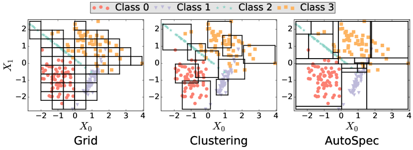
Figure 2: Visualization of the specification set generated by different algorithms.

We present a visualization of the specifications generated by different algorithms on a 2D dataset in Figure 2 (specifications as rectangles, data points as dots, and different colors for different points’ corresponding classes). This illustration highlights that AutoSpec achieves the most comprehensive coverage of the input space compared to other methods. The effectiveness and accuracy of these generated specifications are further evaluated in Section §5.

5 Experimental Evaluation

We answer three questions in this section:

• How does AutoSpec perform on diverse datasets, and are the metrics capable of distinguishing different specification generation algorithms?

• How do auto-generated specifications compare with human-designed specifications?

• Are auto-generated specifications useful in downstream tasks, and can they detect anomalies in trained DNNs?

Application	Input Dimension	Methods	Metrics
			#TP	#FP	#FN	Precision (%)	Recall (%)	F1 (%)
Toy Spiral Data	2	Grid	88	1	1	98.87	98.87	98.87
		Clustering	73	2	15	97.33	82.95	89.57
		AutoSpec	89	1	0	98.88	100.00	99.44
Throughput Prediction	4	Human	73,249	7,520	90,606	90.68	44.70	59.88
		Grid	134,280	36,475	620	78.63	99.54	87.86
		Clustering	124,458	46,506	411	72.79	99.67	84.14
		AutoSpec	168,726	2,649	0	98.45	100.00	99.22
Intrusion Detection	78	Grid	—	—	—	—	—	—
		Clustering	2,117,547	314,434	2,970	87.07	99.85	93.02
		AutoSpec	2,395,672	39,279	0	98.39	100.00	99.18
Beam Management	4096	Grid	—	—	—	—	—	—
		Clustering	4,197	24,370	16,433	14.69	20.34	17.06
		AutoSpec	19,451	25,549	0	43.22	100.00	60.46

Table 1: Evaluation results across datasets. Bold and underline indicate the best and second-best results for each dataset.

Datasets. We choose four different datasets: one toy dataset for visualization and three across various systems.

• Toy spiral dataset. The spiral dataset is a synthetic 2D classification dataset (spi, 2022), designed for easy visualization. The dataset has three classes, where each class has 300 data points. The task is to predict one of three classes based on a 2D location $(X_{0},X_{1})$.

• Uplink throughput prediction dataset. Throughput prediction is a critical task in a range of network systems, such as for resource management (Kumar & Singh, 2018; Chien et al., 2019; Fu & Wang, 2022). We use the Colosseum O-RAN Dataset (Bonati et al., 2021), which contains the base station uplink throughput in various situations. We extract the uplink throughput information out and form the dataset. The targeted task is a time series forecasting job, which uses four historical values as input to predict the throughput at the current timestamp. Thus, the specification’s input constraint has four dimensions, while the output constraint has one dimension.

• Intrusion detection dataset. Intrusion detection and prevention systems (IDSs/IPSs) are important in safeguarding against attacks in cyber environments. We experiment with the CIC-IDS2017 dataset (Sharafaldin et al., 2018), a dataset on intrusion detection through classification tasks. The dataset comprises both benign and malicious network traffic, encompassing a variety of attack types. The dataset features labeled network flows with detailed metadata like timestamps and IP addresses. The model input represents these labeled flows as a feature vector of 78 dimensions, and aims to classify them into either benign or malicious categories (e.g., brute force FTP and brute force SSH). The output is typically a single label for each flow, out of nine labels in total. Thus, we will form the specification with an input constraint of 78 dimensions and an output constraint of 1 dimension.

• Beam management dataset. Highly directional millimeter wave (mmWave) radios perform beam management to establish and maintain reliable links. DeepBeam (Polese et al., 2021) proposes to use deep learning models for coordination-free beam management. It releases a dataset that includes signal samples (I/Q samples) under various conditions, with features like different transmitter beams and receiver gain levels. The DeepBeam model uses these samples as input feature vectors, which have 4096 dimensions in total for beam classification. The output will be classified as transmit beam information, a single-dimension value about the label information.

Data processing. All the above datasets are originally designed for training deep learning models. Instead, we use them to automatically generate specifications that could regularize model behaviors. We split each dataset into two folds in a 9:1 ratio: the first is used for specification generation, and the remainder is used for evaluating the generated specifications.

Metrics. In the following experiments, we use the metrics defined by our framework (§3): TP, FP, FN, precision, recall, and F1 score.

5.1 AutoSpec’s performance

Baselines. We employ the fix-sized grid (“Grid”) and clustering-based methods (“Clustering”) as the baseline algorithms. For the fix-sized grid algorithm, we choose $\beta$ to be $10$; for the clustering algorithm, we employ $k$-means as the clustering method. Regarding the number of clusters, after tuning the parameters, we use 30, 100, 1000, 1000 for spiral, uplink throughput, intrusion detection, and beam management tasks, respectively. We also ask a human expert to define specifications for the throughput prediction task. The expert is unable to define specifications for other tasks like intrusion detection and beam management because the input feature spaces are too complicated. To ensure the generated specification has a tight output range, we set $\alpha$ to $10\%$.

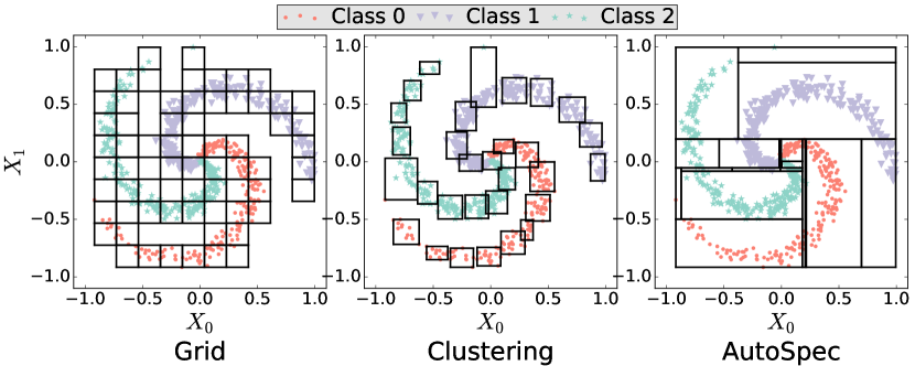
Figure 3: Specification visualization on spec gen dataset.

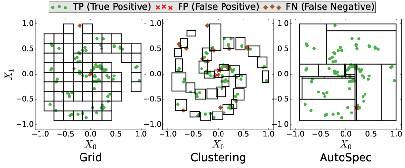
Figure 4: Specification visualization on spec eval dataset.

Results. We run AutoSpec and baselines on the four datasets. Table 1 shows the results. We observe that AutoSpec performs consistently the best across all datasets and applications. Overall, AutoSpec improves the F1 score over the second best by 18% on average.

In the first two datasets, where input dimensions are small, the Grid algorithm also achieves good performance. However, for intrusion detection and beam management, due to the high-dimensional input space, the Grid’s time complexity grows exponentially, and it times out when producing specifications. Specifically, the algorithm was allowed to run for 6 hours on a 64-Core Processor before being terminated, yet it failed to produce specifications within this timeframe. Clustering algorithm performs worse than the Grid and AutoSpec, but it runs fast (in polynomial time) and can generate specifications for high-dimensional spaces. We also observe on the beam management dataset, that both Clustering and AutoSpec’s performance drops significantly. Our hypothesis is that the problem is fundamentally hard with an increased number of input dimensions. This suggests future work of building algorithms for high-dimensional inputs.

A closer look at auto-generated specifications. To better illustrate the generated specifications, we visualize the toy spiral dataset: Figure 4 and Figure 4 depict specifications (rectangles), data points (dots), and points’ corresponding classes (colors). Figure 4 plots the specification generation dataset. From the figure, we observe that neither Clustering nor Grid considers the information in label space while they are splitting the feature space to formulate the specifications. Some specifications contain data points from multiple classes, leading to FPs in the specification evaluation phase. We also observe that AutoSpec splits the input space into subspaces and generates specifications using each subspace, leading to a high recall. Meanwhile, all specifications created by AutoSpec only contain data from one class and thus achieve a high precision.

5.2 Comparison with human-defined specifications

We compare AutoSpec-generated specifications against human-defined ones for the throughput prediction dataset. To accommodate the tight output constraint in specifications, continuous throughput values are divided into ten intervals (0–9), with each interval representing a percentage range of the maximum throughput (e.g., 0 for 0–10% of Throughput${}_{\text{max}}$). This allows us to only have to choose a label to represent the output range for a specification.

The human-defined specifications are designed with two principles: (a) monotonic trend: when historical throughputs show a monotonic increase or decrease, it is expected that the current throughput will follow this trend. Linear regression is employed to fit the previous data and predict the output to a label; (b) stable trend: if the historical throughput values remain steady, it is highly probable that the next throughput will be similar.

The human-defined specification set is generated by iterating through all possible combinations and selecting the ones that satisfy the principles. The details are included in Appendix B, where Table 2 presents three specification examples. Then, we compare the human-defined specifications with AutoSpec-generated ones and show in the results Figure 5. We observe that AutoSpec outperforms human-defined specifications by 39% on F1 score. Human-defined specifications, despite having a high precision, also yield a low recall. This is not surprising, as human experts can only think of specifications for a small number of scenarios and have difficulty covering all possible cases.

Type	x[0]	x[1]	x[2]	x[3]	y(Prediction)
Monotonic Increase	0	2	4	6	8
Monotonic Decrease	9	7	5	3	1
Stable	0	0	0	0	0

Table 2: Examples of human-defined specifications.

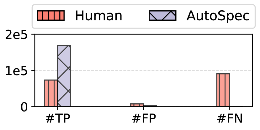
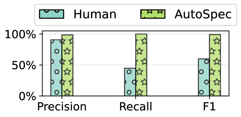
Figure 5: Human-defined specifications vs. AutoSpec-generated specifications.

5.3 Verifying DNNs with generated specifications

Verification engine. To verify neural networks with the generated specifications, we use auto_LiRPA (Xu et al., 2020, 2021; Wang et al., 2021) as our verification engine, which allows automatic bound derivation and computation for general computational graphs.

Experiment setup. The goal is to verify a trained neural network against AutoSpec-generated specifications to identify potential vulnerabilities. For the experiment, we use the same dataset—throughput prediction dataset—for both training the model and generating the specifications. The model is a simple four-layer fully connected neural network with ReLU, with 4, 10, 5, and 1 neurons in each layer. We terminate the training when its loss stabilizes and loss variation $\leq 1\times 10^{-3}$. Then, we start the verification. If the model fails the verification, we extract data points that violate the specifications. These points, termed as counterexamples, highlight cases when the model’s behavior deviates from the expected outcomes.

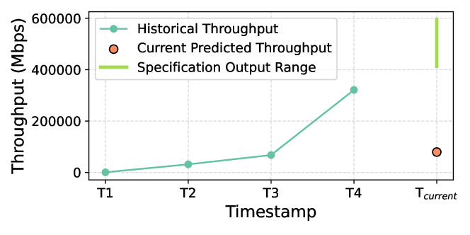
Figure 6: Monotonic increase counterexample.

Detected anomalies. An illustrative counterexample is presented in Figure 6. Analysis of the historical throughput values suggests a monotonically increasing trend. However, the model’s predictions, contrastingly, indicate a substantial decrease, as depicted by the red point (the specification’s expected output range is described by the green line). This discrepancy not only flags an anomaly but also exposes underlying vulnerabilities within the model. We discuss additional counterexamples in Appendix C.

6 Discussion

In this section, we discuss some of the motivations and questions in this work.

6.1 Why learn from data?

In the context of machine learning systems, some previous works propose utilizing specifications to verify neural network safety before deployment into the system (Eliyahu et al., 2021; Wei et al., 2023). However, all these previous works heavily rely on human experts to define the specification set, and these specification sets are often loose and can have errors. Considering the procedure of human experts in defining the specifications, they rely on their understanding of the system and their historical observation of the system behavior. Such an observation procedure can be considered as a step to learn from experience/data, which is a natural task for machine learning to automatically learn from data.

6.2 Correctness of learned specifications

Traditionally, specifications defined by domain experts have been considered as ground-truth laws that must not be violated. However, these expert-defined specifications are inherently limited by human experience and may occasionally be incorrect or incomplete. In contrast, our work proposes a data-driven approach to specification generation. While this method offers the potential to uncover patterns overlooked by human experts, it also introduces the risk of generating incorrect or spurious specifications, especially if the dataset contains noise or biases. To mitigate this risk, we could employ rigorous evaluation and filtering processes, selecting only those specifications that demonstrate a high probability of correctness based on our evaluation criteria. These high-confidence, data-derived specifications are then used to guide and constrain neural network behavior, potentially leading to more robust and reliable models.

6.3 Why Decision Trees?

Our specification generation methods utilize decision trees due to their inherent advantages in this context. Decision trees naturally partition the input space, aligning with our goal of generating hyperrectangle based specifications. Their hierarchical structure offers interpretability, crucial for understanding and validating derived rules. Recent studies have shown decision trees can perform comparably to traditional neural networks in certain tasks (Meng et al., 2019; Zhuang et al., 2024).

7 Conclusion

Formal verification of neural networks offers significant potential for ensuring the safety and reliability of learning-augmented systems. However, current verification frameworks rely on human experts to manually design specifications, a process that is error-prone, incomplete, and unscalable. This paper presents AutoSpec, the first framework to automatically generate specifications for neural networks in learning-augmented systems, alongside a set of evaluation metrics to quantify the quality of these generated specifications. Experimental results across four diverse datasets demonstrate that AutoSpec outperforms both expert-defined specifications and baseline methods.

Appendix A Pseudo code for specification generation algorithms

In this section, we present the pseudo-code for grid-based and clustering-based specification generation algorithms.

Input : Dataset $X_{\text{gen}}$, $Y_{\text{gen}}$, Step size vector $t$, Task Type $task$, Input Feature Dimension:$N$

Output : Set of Specifications $Specs$

1 Initialize $Specs\leftarrow\emptyset$;

2 Compute $x^{\text{min}}$ and $x^{\text{max}}$ from $X_{\text{gen}}$;

3 for $p_{1}$ in range $x^{\text{min}}_{1}$ to $x^{\text{max}}_{1}$ with step size $t_{1}$ do

4       …

5       for $p_{N}$ in range $x^{\text{min}}_{N}$ to $x^{\text{max}}_{N}$ with step size $t_{N}$ do

6            

7            Define rectangle $R\leftarrow\prod_{j=1}^{N}[p_{j},p_{j}+t_{j}]$;

8             $spec\leftarrow$ extractSpecification($R$, $X{\text{gen}}$, $Y_{\text{gen}}$, $task$);

9             if $spec$ is not None then

10                   Add $spec$ to $Specs$;

11             end if

12            

13       end for

14      …

15      

16 end for

17

return $Specs$

Algorithm 3 Grid-based Generation

Input : Feature set $X_{\text{gen}}$, Labels $Y_{\text{gen}}$, Number of clusters $k$, Task Type $task$

Output : Set of Specifications $Specs$

1 Initialize $Specs\leftarrow\emptyset$;

2 Apply clustering algorithm to $X_{\text{gen}}$ forming clusters $\textbf{C}=[C_{1},C_{2},\ldots,C_{k}]$;

3 for each cluster $C_{i}$ do

4       Compute $x^{\text{min}}_{C_{i}}$ and $x^{\text{max}}_{C_{i}}$ for cluster $C_{i}$ in C;

5       Define rectangle $R_{C_{i}}\leftarrow\prod_{j=1}^{n}[x^{\text{min}}_{C_{i},j},x^{\text{max}}_{C_{i},j}]$;

6       $spec\leftarrow$ extractSpecification($R_{C_{i}}$, $X_{\text{gen}}$, $Y_{\text{gen}}$, $task$);

7       if $spec$ is not None then

8             Add $spec$ to $Specs$;

9            

10       end if

11      

12 end for

return $Specs$

Algorithm 4 Clustering-based Generation

Appendix B Human Defined Specification

This section outlines examples of human-designed specifications. Each specification has been translated into actual throughput speeds, based on the highest observed throughput of 919264 Mbps. The labels from “0” to “9” represent different ranges of throughput. For example, label “0” means the throughput is between 0 and 91926.4 Mbps. Each label after “0” covers an equally sized higher range of speeds, all the way up to the top speed. We list parts of our specifications in Table 3.

Type	x[0]	x[1]	x[2]	x[3]	y (Prediction)
Stable	0	0	0	0	0
Increasing	0	1	2	3	4
Increasing	0	1	2	4	5
Increasing	0	1	2	5	6
Increasing	0	1	2	6	7
Increasing	2	4	5	7	8
Decreasing	5	4	1	0	0
Decreasing	5	4	2	0	0
Decreasing	5	4	2	1	0
Decreasing	9	8	7	6	5
Stable	9	9	9	9	9

Table 3: Examples of human-defined specifications.

Appendix C Counterexamples

We list two main counterexamples revealed by our generated specification set. Figure 8 illustrates an unexpected model behavior: although the anticipated trend for the current timestamp throughput is a continuous increase, the model’s predicted output exhibits a substantial decrease. This deviation from the expected behavior is an anomaly. Conversely, Figure 8 presents the reverse scenario. In this case, despite the projected trend indicating a decrease, the model’s output shows an increase, further underscoring the discrepancies between the expected and actual model behaviors, revealing the vulnerabilities.

Figure 7: Monotonic increase counterexample.

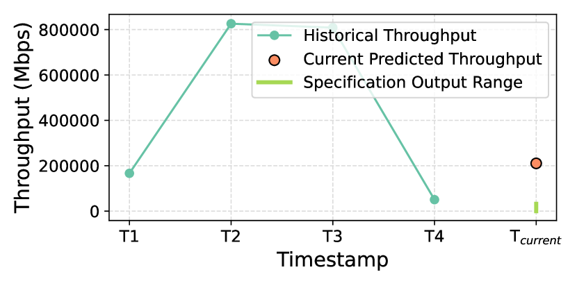
Figure 8: Monotonic decrease counterexample.

References

- spi (2022) Spiral toy dataset, 2022. URL https://cs231n.github.io/neural-networks-case-study/.
- Ammons et al. (2002) Ammons, G., Bodik, R., and Larus, J. R. Mining specifications. ACM Sigplan Notices, 37(1):4–16, 2002.
- Bak & Tran (2022) Bak, S. and Tran, H.-D. Neural network compression of acas xu early prototype is unsafe: Closed-loop verification through quantized state backreachability. In NASA Formal Methods Symposium, pp. 280–298. Springer, 2022.
- Bonati et al. (2021) Bonati, L., D’Oro, S., Polese, M., Basagni, S., and Melodia, T. Intelligence and learning in o-ran for data-driven nextg cellular networks. IEEE Communications Magazine, 59(10):21–27, 2021.
- Chien et al. (2019) Chien, W.-C., Lai, C.-F., and Chao, H.-C. Dynamic resource prediction and allocation in c-ran with edge artificial intelligence. IEEE Transactions on Industrial Informatics, 15(7):4306–4314, 2019.
- Eliyahu et al. (2021) Eliyahu, T., Kazak, Y., Katz, G., and Schapira, M. Verifying learning-augmented systems. In Proceedings of the 2021 ACM SIGCOMM 2021 Conference, pp. 305–318, 2021.
- Fu & Wang (2022) Fu, Y. and Wang, X. Traffic prediction-enabled energy-efficient dynamic computing resource allocation in cran based on deep learning. IEEE Open Journal of the Communications Society, 3:159–175, 2022.
- Geng et al. (2023) Geng, C., Le, N., Xu, X., Wang, Z., Gurfinkel, A., and Si, X. Towards reliable neural specifications. In International Conference on Machine Learning, pp. 11196–11212. PMLR, 2023.
- Jay et al. (2019) Jay, N., Rotman, N., Godfrey, B., Schapira, M., and Tamar, A. A deep reinforcement learning perspective on internet congestion control. In International Conference on Machine Learning, pp. 3050–3059. PMLR, 2019.
- Jin et al. (2024) Jin, S., Zhu, R., Hassan, A., Zhu, X., Zhang, X., Mao, Z. M., Qian, F., and Zhang, Z.-L. Oasis: Collaborative neural-enhanced mobile video streaming. In Proceedings of the 15th ACM Multimedia Systems Conference, pp. 45–55, 2024.
- Katz et al. (2019) Katz, G., Huang, D. A., Ibeling, D., Julian, K., Lazarus, C., Lim, R., Shah, P., Thakoor, S., Wu, H., Zeljić, A., et al. The marabou framework for verification and analysis of deep neural networks. In Computer Aided Verification: 31st International Conference, CAV 2019, New York City, NY, USA, July 15-18, 2019, Proceedings, Part I 31, pp. 443–452. Springer, 2019.
- Kraska et al. (2018) Kraska, T., Beutel, A., Chi, E. H., Dean, J., and Polyzotis, N. The case for learned index structures. In Proceedings of the 2018 international conference on management of data, pp. 489–504, 2018.
- Kumar & Singh (2018) Kumar, J. and Singh, A. K. Workload prediction in cloud using artificial neural network and adaptive differential evolution. Future Generation Computer Systems, 81:41–52, 2018.
- Le & Lo (2018) Le, T.-D. B. and Lo, D. Deep specification mining. In Proceedings of the 27th ACM SIGSOFT International Symposium on Software Testing and Analysis, pp. 106–117, 2018.
- Lemieux et al. (2015) Lemieux, C., Park, D., and Beschastnikh, I. General ltl specification mining (t). In 2015 30th IEEE/ACM International Conference on Automated Software Engineering (ASE), pp. 81–92. IEEE, 2015.
- Liu & Lang (2019) Liu, H. and Lang, B. Machine learning and deep learning methods for intrusion detection systems: A survey. applied sciences, 9(20):4396, 2019.
- Mao et al. (2017) Mao, H., Netravali, R., and Alizadeh, M. Neural adaptive video streaming with pensieve. In Proceedings of the conference of the ACM special interest group on data communication, pp. 197–210, 2017.
- Mao et al. (2019) Mao, H., Schwarzkopf, M., Venkatakrishnan, S. B., Meng, Z., and Alizadeh, M. Learning scheduling algorithms for data processing clusters. In Proceedings of the ACM special interest group on data communication, pp. 270–288. 2019.
- Meng et al. (2019) Meng, Z., Chen, J., Guo, Y., Sun, C., Hu, H., and Xu, M. Pitree: Practical implementation of abr algorithms using decision trees. In Proceedings of the 27th ACM International Conference on Multimedia, pp. 2431–2439, 2019.
- Polese et al. (2021) Polese, M., Restuccia, F., and Melodia, T. DeepBeam: Deep Waveform Learning for Coordination-Free Beam Management in mmWave Networks. Proc. of ACM International Symposium on Mobile Ad Hoc Networking and Computing (MobiHoc), 2021.
- Sharafaldin et al. (2018) Sharafaldin, I., Lashkari, A. H., and Ghorbani, A. A. Toward generating a new intrusion detection dataset and intrusion traffic characterization. ICISSp, 1:108–116, 2018.
- Tan et al. (2021) Tan, C., Zhu, Y., and Guo, C. Building verified neural networks with specifications for systems. In Proceedings of the 12th ACM SIGOPS Asia-Pacific Workshop on Systems, pp. 42–47, 2021.
- Wang et al. (2021) Wang, S., Zhang, H., Xu, K., Lin, X., Jana, S., Hsieh, C.-J., and Kolter, J. Z. Beta-CROWN: Efficient bound propagation with per-neuron split constraints for complete and incomplete neural network verification. Advances in Neural Information Processing Systems, 34, 2021.
- Wei et al. (2023) Wei, T., Liu, C., Jia, Z., and Tan, C. Building verified neural networks for computer systems with ouroboros. Proceedings of Machine Learning and Systems, 5, 2023.
- Wu et al. (2022) Wu, H., Barrett, C., Sharif, M., Narodytska, N., and Singh, G. Scalable verification of gnn-based job schedulers. Proceedings of the ACM on Programming Languages, 6(OOPSLA2):1036–1065, 2022.
- Xu et al. (2020) Xu, K., Shi, Z., Zhang, H., Wang, Y., Chang, K.-W., Huang, M., Kailkhura, B., Lin, X., and Hsieh, C.-J. Automatic perturbation analysis for scalable certified robustness and beyond. Advances in Neural Information Processing Systems, 33, 2020.
- Xu et al. (2021) Xu, K., Zhang, H., Wang, S., Wang, Y., Jana, S., Lin, X., and Hsieh, C.-J. Fast and Complete: Enabling complete neural network verification with rapid and massively parallel incomplete verifiers. In International Conference on Learning Representations, 2021. URL https://openreview.net/forum?id=nVZtXBI6LNn.
- Yan et al. (2020) Yan, F. Y., Ayers, H., Zhu, C., Fouladi, S., Hong, J., Zhang, K., Levis, P., and Winstein, K. Learning in situ: a randomized experiment in video streaming. In 17th USENIX Symposium on Networked Systems Design and Implementation (NSDI 20), pp. 495–511, 2020.
- Zhuang et al. (2024) Zhuang, Y., Liu, L., Singh, C., Shang, J., and Gao, J. Learning a decision tree algorithm with transformers. arXiv preprint arXiv:2402.03774, 2024.