3DIOC: Direct Data-Driven Inverse Optimal Control for LTI Systems

Abstract

This paper develops a direct data-driven inverse optimal control (3DIOC) algorithm for the linear time-invariant (LTI) system who conducts a linear quadratic (LQ) control, where the underlying objective function is learned directly from measured input-output trajectories without system identification. By introducing the Fundamental Lemma, we establish the input-output representation of the LTI system. We accordingly propose a model-free optimality necessary condition for the forward LQ problem to build a connection between the objective function and collected data, with which the inverse optimal control problem is solved. We further improve the algorithm so that it requires a less computation and data. Identifiability condition and perturbation analysis are provided. Simulations demonstrate the efficiency and performance of our algorithms.

I Introduction

Inverse optimal control (IOC) is to identify the underlying objective function of an optimal control system based on its input and output trajectories [1]. It is also known as inverse reinforcement learning (IRL) in the machine learning community, as an important branch of learning from demonstration (LfD) methods [2]. IOC is widely applied in autonomous driving [3] and human-robot collaborations [4], where the learned objective function is used for human intention (or trajectory) prediction. Another application is the imitation learning for robots [5]. With the identified objective, the task imitation generalizes well in different environments.

Previous studies on IOC usually assume the form of the objective function and the system dynamic model are known as the prior knowledge. One common option for optimal control objective function is the linear quadratic form. [6] studies the inverse infinite-time linear quadratic regulator (LQR) control assuming the constant feedback gain matrix is already known. For the finite-time LQR, [7] identifies the weighting matrices in objective function for continuous case and [8, 9] solve the discrete case. A more general assumption for objective function is a weighted sum of specified features [10]. However, the exact system model is difficult to obtain in the practice, restricting the application of traditional IOC algorithms. System identification can be conducted as a pre-process (also called indirect data-driven methods), while the identification error may affect the learning performance to the objective function in an unexpected way [11].

Model-free IOC remains an issue that has not been fully resolved. Some efforts have been made under the Markov decision process (MDP) in IRL framework [12, 13]. Inspired by the deep Koopman representation of the unknown system, [14] proposes an IOC algorithm to achieve an optimal Koopman operator and the unknown weights estimation together through iterations. However, this method is expensive in computation and requires substantial observation data due to the iterative framework.

Motivated by the above discussion, we develop a novel direct data-driven IOC algorithm. The main challenge lies in how to identify the objective function with less data and computational cost, and the identifiability analysis to the ill-posed inverse problem. We innovatively introduce the fundamental lemma from the behavioral system theory [15], which demonstrates that an LTI system can be equally represented by its collected input-output trajectories under certain persistent excitation conditions. With this input-output representation, we establish the model-free Karush–Kuhn–Tucker (KKT) condition for LQ control and build the IOC problem with this optimality necessary condition. We further remove the redundant parameters in the representation to improve the estimation efficiency and robustness. The proposed 3DIOC requires a small amount of data including one offline stochastic trajectory and one optimal trajectory, and only needs to solve a quadratic programming (QP) once. The main contributions are summarized as follows:

• We propose a direct data-driven IOC approach of LQ control for LTI systems. Based on the input-output representation, the IOC problem is built using established model-free KKT conditions as a constraint. After removing the redundant parameter in the representation, a simplified 3DIOC is developed which requires less computation and observation data.

• We provide the identifiability condition to deal with the ill-posedness of the inverse problem. When the observation is disturbed by noises, the infeasible case is considered and the perturbation analysis is derived.

• Numerical simulations demonstrate the computation efficiency and identification performance of the proposed algorithm, also showing the improvement as a result of removing the redundant parameter.

The remainder of the paper is organized as follows. Section II introduces the preliminaries and describes the problem of interest. Section III provides the main results and algorithms. Simulation experiments are shown in Section IV, followed by the conclusion in Section V.

Notations: For a matrix $A\in\mathbb{R}^{n\times m}$, $A^{\dagger}$ denotes its Moore-Penrose pseudo inverse. $A(i:j,:)$ (or $A(:,i:j)$) denotes the matrix composed by the $i$ to $j$ rows (or columns). $A\otimes B$ is the Kronecker product between matrices $A$ and $B$. $\operatorname{vech}(A)\in\mathbb{R}^{\frac{1}{2}n(n+1)}$ represents the half-vectorization of a symmetric matrix $A\in\mathbb{S}^{n}$. For a series of vectors $v_{1},\dots,v_{k}$, $\operatorname{col}(v_{1},\dots,v_{k})=(v_{1}^{T},\dots,v_{k}^{T})^{T}$. $\operatorname{diag}(v)$ represents the diagonal matrix made by the vector $v$. $\operatorname{diag}(A_{1},\dots,A_{k})$ is the block diagonal matrix composed of matrices $A_{1},\dots,A_{k}$ and $\operatorname{col}(A_{1},\dots,A_{k})=(A_{1}^{T},\dots,A_{k}^{T})^{T}$. $w\wedge w^{\prime}$ denotes the concatenation of two trajectories $w,w^{\prime}$.

II Preliminaries and Problem Formulation

II-A Problem Description

Consider an LTI system $\mathscr{B}$

$$x_{k+1}=Ax_{k}+Bu_{k},~{}y_{k}=Cx_{k}+Du_{k},$$ (1)

where $A\in\mathbb{R}^{n\times n},B\in\mathbb{R}^{n\times m},C\in\mathbb{R}^{p\times n},D\in\mathbb{R}^{p\times m}$, and $x_{k},u_{k},y_{k}$ are respectively the system state, control input and output at time $k$. The lag of the system is $l$. Denote all the $L$-length input-output trajectories generated by $\mathscr{B}$ as a set $\mathscr{B}|_{L}$. We have the following assumptions throughout the paper:

Assumption 1 (Model-free).

We have no prior knowledge about the dynamic matrices $A,B,C,D$ in (1). But one input-output trajectory

$$w^{d}:=\{u^{d}_{k},y^{d}_{k}\}_{k=0}^{T-1},~{}w^{d}\in\mathscr{B}|_{T}$$ (2)

of length $T$ is available.

Assume the system $\mathscr{B}$ in (1) is driven by a forward optimal LQ controller. The LQ problem is given as:

$$\mathbf{P}_{0}:\begin{aligned} &\min_{u_{0:N^{\prime}-1},y_{0:N^{\prime}-1}}~{}\sum_{k=0}^{N^{\prime}-1}y_{k}^{T}Qy_{k}+u_{k}^{T}Ru_{k}\\ &~{}~{}~{}~{}~{}~{}~{}s.t.~{}~{}~{}~{}~{}~{}~{}~{}\eqref{sys},x_{0}=\bar{x},\end{aligned}$$ (3)

where $R\in\mathbb{S}^{m}$ is a positive definite matrix, $Q\in\mathbb{S}^{p}$ is a positive semi-definite matrix and $\bar{x}$ is the initial state. $N^{\prime}$ is the control horizon. We have access to an optimal input-output trajectory denoted by

$$w^{o}:=\{u^{o}_{k},y^{o}_{k}\}_{k=0}^{N^{\prime}-1},~{}w^{o}\in\mathscr{B}|_{N^{\prime}}.$$ (4)

The inverse problem tackled in this paper is described as follow.

Problem 1.

The direct data-driven IOC problem is to identify the weighting matrices $Q,R$ in the control objective function in problem $\mathbf{P}_{0}$ directly from collected trajectories $w^{d},w^{o}$.

II-B Fundamental Lemma

In order to build the direct data-driven IOC problem, we introduce the Fundamental Lemma from the behavioural system theory as a preliminary. Behavioural system theory views the LTI dynamic system as a subspace of the signal space in which the system trajectories live. We first define a persistently exciting property for the input $u^{d}$.

Definition 1.

The input signal $u^{d}=\{u^{d}_{k}\}_{k=0}^{T-1}$ is persistently exciting of order $L$ if the corresponding Hankel matrix

$$\mathcal{H}_{L}(u^{d}):=\begin{pmatrix}u^{d}_{0}&\cdots&u^{d}_{T-L}\\ \vdots&\ddots&\vdots\\ u^{d}_{L-1}&\cdots&u^{d}_{T-1}\end{pmatrix}$$

has full row rank, where $L,T\in\mathbb{Z}$ and $T\geq L$.

Based on Definition 1, the Fundamental Lemma is as follows.

Lemma 1.

(Fundamental Lemma [16]) Consider the linear time-invariant system $\mathscr{B}$ in (1). If
a) system $\mathscr{B}$ is controllable,  b) $w^{d}\in\mathscr{B}|_{T}$,
c) the inputs $u^{d}$ is persistently exciting of order $L+n$,
then we have

$$\mathscr{B}|_{L}=\mathrm{image}~{}\mathcal{H}_{L}(w^{d}),$$ (5)

where

$$\mathcal{H}_{L}(w^{d})=\begin{pmatrix}\operatorname{col}(u_{0}^{d},y_{0}^{d})&\cdots&\operatorname{col}(u_{T-L}^{d},y_{T-L}^{d})\\ \vdots&\ddots&\vdots\\ \operatorname{col}(u_{L-1}^{d},y_{L-1}^{d})&\cdots&\operatorname{col}(u_{T-1}^{d},y_{T-1}^{d})\end{pmatrix}.$$

This lemma reveals that under three conditions a)-c), any $L$-length trajectory generated by $\mathscr{B}$ can be represented through a linear combination of the columns of $\mathcal{H}_{L}(w^{d})$. The image of $\mathcal{H}_{L}(w^{d})$ is an input-ouput representation of $\mathscr{B}$.

Lemma 2.

(Corollary 19, [17]) Consider the LTI system $\mathscr{B}$ in (1). For $L\geqslant\max(l,n)$ and the trajectory $w^{d}$, we have $\mathscr{B}|_{L}=\mathrm{image}~{}\mathcal{H}_{L}(w^{d})$ if and only if

$$\operatorname{rank}(\mathcal{H}_{L}(w^{d}))=mL+n.$$ (6)

Lemma 2 is a generalization of the Fundamental Lemma, which provides a sufficient and necessary condition and does not require the controllability of the system. Equation (6) is called a generalized persistency of excitation (PE) condition. We will utilize Lemma 2 to establish the input-output representation for $\mathscr{B}$ with $w^{d}$ in the following section.

III Direct Data-Driven IOC

In this section, we firstly derive the model-free KKT condition for the LQ problem $\mathbf{P}_{0}$ based on the input-output representation introduced in the preliminary. We build the direct data-driven IOC problem with the obtained optimality necessary condition. Then we simplify the algorithm by removing the redundant parameters in the representation.

III-A Model-free KKT Condition

To obtain the model-free KKT condition, we firstly reformulate the problem $\mathbf{P}_{0}$ into a data-enabled LQ control.

For the collected optimal trajectory $w^{o}$ in (4), we split it as an initial trajectory of length $T_{ini}$ and the remaining sequence of length $N=N^{\prime}-T_{ini}$, which is

$$w^{o}=w^{ini}\wedge\tilde{w},~{}w^{ini}\in\mathscr{B}|_{T_{ini}},~{}\tilde{w}\in\mathscr{B}|_{N},$$ (7)

where we denote the $w^{ini}=\{u^{ini}_{k},y^{ini}_{k}\}_{k=0}^{T_{ini}-1}$ and $\tilde{w}=\{\tilde{u}_{k},\tilde{y}_{k}\}_{k=0}^{N-1}$. The following lemma guarantees the uniqueness of the initial state for a $T_{ini}$-length trajectory $w^{d}$ with inputs.

Lemma 3.

(Lemma 1, [18]) For a trajectory $w^{ini}\in\mathscr{B}|_{T_{ini}}$ and an arbitrary $N$-length input sequence $\{u_{k}\}_{k=0}^{N-1}$, if $T_{ini}\geqslant l$, there exists a unique initial state $x_{0}^{ini}$ and unique outputs $\{y_{k}\}_{k=0}^{N-1}$, such that $w^{ini}\wedge w\in\mathscr{B}|_{T_{ini}+N}$.

Similarly, for the measured trajectory $w^{d}$, we define

$$\begin{pmatrix}U_{p}\\ U_{f}\end{pmatrix}:=\mathcal{H}_{T_{ini}+N}(u^{d}),\begin{pmatrix}Y_{p}\\ Y_{f}\end{pmatrix}:=\mathcal{H}_{T_{ini}+N}(y^{d}),$$

where $U_{p}$ is the first $T_{ini}$ row of Hankel matrix $\mathcal{H}_{T_{ini}+N}(u^{d})$ and $U_{f}$ is the remaining $N$ row (similarly for $Y_{p}$ and $Y_{f}$). Then we build an offline data matrix based on $w^{d}$

$$H_{T_{ini}+N}(w^{d})=:\operatorname{col}(U_{p},Y_{p},U_{f},Y_{f})\sim\mathcal{H}_{T_{ini}+N}(w^{d}).$$ (8)

Therefore, according to Lemma 2, if $T_{ini}+N\geqslant\max(l,n)$, we have the following statement for $w^{d}$.

Proposition 1.

The data matrix $H_{T_{ini}+N}(w^{d})$ is an input-output representation of system $\mathscr{B}$ if the trajectory $w^{d}$ satisfies the generalized PE condition (6) which is

$$\operatorname{rank}(H_{T_{ini}+N}(w^{d}))=m(T_{ini}+N)+n.$$ (9)

Based on above discussions, we build the data-enabled LQ problem given $w^{d}$ and $w^{ini}$:

$$\mathbf{P}_{1}:\begin{aligned} &\min_{g,u,y}~{}~{}~{}y^{T}\mathcal{Q}y+u^{T}\mathcal{R}u\\ &~{}s.t.~{}~{}~{}\operatorname{col}(U_{p},Y_{p},U_{f},Y_{f})g=\operatorname{col}(u^{ini},y^{ini},u,y),\end{aligned}$$ (10)

where $y=\operatorname{col}(y_{0},y_{1},\dots,y_{N-1}),u=\operatorname{col}(u_{0},u_{1},\dots,u_{N-1})$ and $\mathcal{Q}=\operatorname{diag}(Q,\dots,Q),\mathcal{R}=\operatorname{diag}(R,\dots,R)$. In the constraint, $g$ serves as a decision variable. If (9) is satisfied, the right side is guaranteed to be optimal in the trajectory set $\mathscr{B}|_{T_{ini}+N}$. If $T_{ini}\geqslant l$, one solution $u$ combined with $u^{ini},y^{ini}$ ensures one unique output $y$.

Proposition 2.

If equation (9) and $T_{ini}\geqslant l$ are fulfilled, the $N$-length trajectory $\tilde{w}$ split from $w^{o}$ is exactly an optimal solution to problem $\mathbf{P}_{1}$.

Proposition 2 reveals a connection between the optimal solutions of $\mathbf{P}_{0}$ and $\mathbf{P}_{1}$. With the formulation of $\mathbf{P}_{1}$, we establish its model-free KKT conditions as follows.

Lemma 4 (Model-free KKT).

The optimal input solution $u^{*}$ with its corresponding decision variable $g^{*}$ and output trajectory $y^{*}$ to $\mathbf{P}_{1}$ satisfy

$$\frac{\partial L}{\partial g}={\lambda^{*}}^{T}H_{T_{ini}+N}(w^{d})=0,$$ (11)

$$\frac{\partial L}{\partial u}=2\mathcal{R}u^{*}-\lambda_{u}^{*}=0,\frac{\partial L}{\partial y}=2\mathcal{Q}y^{*}-\lambda_{y}^{*}=0,$$

$$\frac{\partial L}{\partial\lambda}=H_{T_{ini}+N}(w^{d})g^{*}-\operatorname{col}(u^{ini},y^{ini},u^{*},y^{*})=0,$$

where $L$ denotes the Lagrangian function

$$L(g,u,y,\lambda)= y^{T}\mathcal{Q}y+u^{T}\mathcal{R}u+\lambda^{T}({H}_{T_{ini}+N}(w^{d})g$$

$$-\operatorname{col}(u^{ini},y^{ini},u,y)),$$

and for the costate we denote $\lambda=\operatorname{col}(\lambda_{ini},\lambda_{u},\lambda_{y})$.

Denote $w_{p}=\operatorname{col}(U_{p},Y_{p})$. From Lemma 4, we derive

$$H_{T_{ini}+N}^{T}(w^{d})\lambda^{*}=({U_{p}^{T}~{}~{}Y_{p}^{T}}~{}~{}U_{f}^{T}~{}~{}Y_{f}^{T})\operatorname{col}(\lambda^{*}_{ini},\lambda^{*}_{u},\lambda^{*}_{y})$$

$$=w_{p}^{T}\lambda_{ini}+U_{f}^{T}(2\mathcal{R}u^{*})+Y_{f}^{T}(2\mathcal{Q}y^{*})=0.$$

According to Proposition 2, the optimal trajectory $\tilde{w}$ split from $w^{o}$ should also satisfy Lemma 4, which is

$$w_{p}^{T}\lambda_{ini}+2U_{f}^{T}(\mathcal{R}\tilde{u})+2Y_{f}^{T}(\mathcal{Q}\tilde{y})=0$$ (12)

III-B Vanilla 3DIOC

Equation (12) presents an equality constraint for the real weighting matrices $Q,R$ along with the collected input-output data $w^{d},w^{o}$, which can be used to estimate matrices directly from the data. However, by observing (12), we find the identification to $Q,R$ possesses a scalar ambiguity property.

Definition 2 (Scalar Ambiguity).

Given the collected data $w^{d}$ and optimal trajectory $w^{o}$, two weighting matrix sets $(Q,R)$ and $(\alpha Q,\alpha R)$ with an arbitrary scalar $\alpha\in\mathbb{R}_{+}$ all satisfy the equation (12).

Additionally, we have to point out that the inverse problem (Problem 1) is actually ill-posed, which means there may exist multiple linearly independent matrix sets of $(Q,R)$ that can generate the same optimal trajectory $w^{o}$. Therefore, we provide the following condition to ensure the identifiability.

Theorem 1 (Identifiability).

Suppose there are two sets of weighting matrix $(Q,R)$ and $(Q^{\prime},R^{\prime})$ both satisfying equation (12) with respect to collected data $w^{d},w^{o}$ and equation (9) is fulfilled. We have $Q=\alpha Q^{\prime},R=\alpha R^{\prime}$ for a scalar $\alpha\in\mathbb{R}_{+}$, if

$$\operatorname{rank}(\tilde{\Psi})=(m+p)T_{ini}+\frac{1}{2}(m^{2}+m+p^{2}+p)-1,$$ (13)

The matrix $\tilde{\Psi}$ is defined by $w^{d},w^{o}$ in Appendix A.

Proof.

See the proof in Appendix A. ∎

Appendix A provides the explicit calculation form of $\tilde{\Psi}$ and it is easy to check in the practice.

With the identifiability guarantee, we can obtain a solution as the real weighting matrices multiplying a scalar. Utilizing equation (12) as a constraint, given $w^{d},w^{o}$, we provide the following direct data-driven IOC problem:

Problem 2 (Direct Data-driven IOC Problem).

$$\min_{\lambda_{ini},Q,R}~{}~{}\alpha^{2}$$ (14)

$$~{}~{}~{}s.t.~{}~{}~{}~{}~{}\eqref{kkt_cons},I\preceq\mathrm{diag}(Q,R)\preceq\alpha I.$$

To avoid the scalar ambiguity, we minimize the condition number of the matrix $\operatorname{diag}(Q,R)$. Thus, if the collected data is accurate (without observation noises), the Problem 2 is a feasible LMI problem. Since it is convex with linear constraints, there exists a unique optimal solution.

Note that when the identifiability condition (13) is satisfied, Problem 2 is feasible. However, in the practical scenario, the data collection is usually disturbed by observation noises, leading to the full rank of $\tilde{\Psi}$. Therefore, we provide the following Problem 3 to deal with this infeasible case.

Problem 3 (Infeasible Case).

$$\min_{\lambda_{ini},Q,R}~{}\|w_{p}^{T}\lambda_{ini}+2U_{f}^{T}\mathcal{R}\tilde{u}+2Y_{f}^{T}\mathcal{Q}\tilde{y}\|_{2}^{2}$$ (15)

$$~{}~{}~{}s.t.~{}~{}~{}~{}\|\operatorname{col}(\lambda_{ini},\operatorname{vech}(Q),\operatorname{vech}(R))\|_{2}^{2}=1.$$

III-C Simplified 3DIOC without Redundant Variables

Notice that the unknown variables in problem $\mathbf{P}_{1}$ are actually redundant. We do not care the estimation of the Lagrangian multiplier $\lambda_{ini}$ and the number of variables in it will increase when $T_{ini}$ goes larger, leading to an unnecessary cost in computation. Therefore, in this subsection, we present a simplified 3DIOC by removing the redundant variables.

Substitute optimization variables $y,g$ with $u$ in problem $\mathbf{P}_{1}$ by converting the constraint into

$$y=Y_{f}\begin{pmatrix}U_{p}\\ Y_{p}\\ U_{f}\end{pmatrix}^{\dagger}\begin{pmatrix}u^{ini}\\ y^{ini}\\ u\end{pmatrix}\!=\!K\begin{pmatrix}u^{ini}\\ y^{ini}\\ u\end{pmatrix}\!=\!(K_{p}~{}|~{}K_{f})\begin{pmatrix}z_{ini}\\ u\end{pmatrix}\vspace{-3pt}$$ (16)

in which case the objective function becomes

$$J(u)=:\begin{pmatrix}z_{ini}^{T}&u^{T}\end{pmatrix}\begin{pmatrix}K_{p}^{T}\\ K_{f}^{T}\end{pmatrix}\mathcal{Q}\begin{pmatrix}K_{p}&K_{f}\end{pmatrix}\begin{pmatrix}z_{ini}\\ u\end{pmatrix}+u^{T}\mathcal{R}u$$

$$=z_{ini}^{T}K_{p}^{T}\mathcal{Q}K_{p}z_{ini}\!+\!2z_{ini}^{T}K_{p}^{T}\mathcal{Q}K_{f}u\!+\!u^{T}(K_{f}^{T}\mathcal{Q}K_{f}\!+\!\mathcal{R})u,$$

and problem $\mathbf{P}_{1}$ turns into an unconstrained problem

$$\mathbf{P}_{2}:~{}\min_{u}~{}~{}J(u).\vspace{-3pt}$$

Therefore, the optimality necessary condition is the derivation of $J(u)$ with respect to $u$ equals zero. We have

$$\frac{\partial J(u)}{\partial u}=2(K_{f}^{T}\mathcal{Q}K_{f}+\mathcal{R})u+2K_{f}^{T}\mathcal{Q}^{T}K_{p}z_{ini}.$$

Based on this new formulation, we present the simplified model-free KKT condition.

Lemma 5 (Simplified Model-free KKT).

Given the collected data $w^{d},w^{ini}$, the optimal input solution $u^{*}$ corresponding to $\mathbf{P}_{2}$ satisfies

$$(K_{f}^{T}\mathcal{Q}K_{f}+\mathcal{R})u^{*}+K_{f}^{T}\mathcal{Q}^{T}K_{p}z_{ini}=0.\vspace{-3pt}$$ (17)

Similarly, the optimal trajectory $\tilde{w}$ split from $w^{o}$ also satisfy equation (17), which is

$$(K_{f}^{T}\mathcal{Q}K_{f}+\mathcal{R})\tilde{u}+K_{f}^{T}\mathcal{Q}^{T}K_{p}z_{ini}=0.$$ (18)

With equation (18), we provide a new identifiability condition for $Q,R$ as follows.

Theorem 2 (Identifiability).

Suppose there are two weighting matrix sets $(Q,R)$ and $(Q^{\prime},R^{\prime})$ both satisfy equation (18) with respect to collected data $w^{d},w^{o}$ ensuring equation (9). We have $Q=\alpha Q^{\prime},R=\alpha R^{\prime}$ for a scalar $\alpha\in\mathbb{R}_{+}$, if

$$\operatorname{rank}(\tilde{\Phi})=\frac{1}{2}(m^{2}+m+p^{2}+p)-1,\vspace{-3pt}$$ (19)

The matrix $\tilde{\Phi}$ is defined by $w^{d},w^{o}$ in Appendix B.

Proof.

See the proof in Appendix B. ∎

The identifiable condition (19) is easy to check given the explicit form (30) in the proof. Note that matrix $\tilde{\Phi}$ is of $mN\times\frac{1}{2}(m^{2}+m+p^{2}+p)$. We can further obtain an unidentifiable condition for our inverse problem (Problem 1) as follows.

Corollary 1 (Unidentifiability Condition).

The real weighting matrices $Q,R$ cannot be identified if the horizon $N=N^{\prime}-T_{ini}$ is set to satisfy

$$N<\frac{1}{2m}(m^{2}+m+p^{2}+p)-\frac{1}{m}.\vspace{-3pt}$$

Proof.

If $\operatorname{rank}(\tilde{\Phi})=mN<\frac{1}{2}(m^{2}+m+p^{2}+p)-1$, then there exist multiple linearly independent solution for $Q,R$ with respect to equation (18). ∎

Then with the new constraint (18), the 3DIOC problem with no redundant parameters is formulated as

Problem 4 (Simplified 3DIOC).

$$\min_{Q,R}~{}~{}\alpha^{2}$$ (20)

$$~{}s.t.~{}~{}\eqref{skkt-eq},I\preceq\mathrm{diag}(Q,R)\preceq\alpha I.$$

Problem 4 has a unique optimal solution when the identifiable condition (19) is satisfied. The infeasible case with the existence of the observation noise is solved through the following problem.

Problem 5 (Infeasible Case of Simplified 3DIOC).

$$\min_{Q,R}~{}\|(K_{f}^{T}\mathcal{Q}K_{f}+\mathcal{R})\tilde{u}+K_{f}^{T}\mathcal{Q}^{T}K_{p}z_{ini}\|_{2}^{2}$$ (21)

$$~{}s.t.~{}~{}\|\operatorname{col}(\operatorname{vech}(Q),\operatorname{vech}(R))\|_{2}^{2}=1.$$

Remark 1.

In this simplified 3DIOC formulation, we only need the online optimal input $\tilde{u}$ instead both $\tilde{y},\tilde{u}$ comparing to the former formulations in Problem 2 and 3. Besides, since the number of optimization variables is greatly reduced by $(m+p)T_{ini}$, the solving is more efficient and robust, which will be demonstrated in the simulation part.

For Problem 5, we provide the following perturbation analysis considering the observation noise in the collected data.

Theorem 3 (Perturbation Analysis).

Suppose the online collected data $\tilde{u}$ has a small perturbation $\Delta\tilde{u}$. The real weighting matrices are $Q,R$ and the perturbed estimations are $Q^{\prime},R^{\prime}$. The estimation error is bounded by

$$\|\Theta(Q^{\prime},R^{\prime})-\Theta(Q,R)\|\leqslant\|\sum_{i=1}^{N_{v}-1}\frac{v_{i}^{T}(\Delta\tilde{\Phi}^{T}\tilde{\Phi}+\tilde{\Phi}^{T}\Delta\tilde{\Phi})v_{i}}{\sigma-\sigma_{i}}\|\vspace{-3pt}$$ (22)

where $\sigma_{i},v_{i}$ are eigenvalues and corresponding eigenvectors of matrix $\tilde{\Phi}^{T}\tilde{\Phi}$. $\Theta(Q,R)$ represents $\operatorname{col}(\operatorname{vech}(Q),\operatorname{vech}(R))$. $\Delta\tilde{\Phi}$ is defined in Appendix C.

Proof.

See the proof in Appendix C. ∎

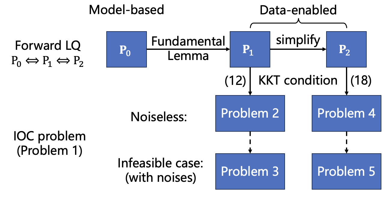
Figure 1: The flow chart of proposed problems.

III-D Special Case for LQR-IOC

$\mathbf{P}_{0}$ is a general LQ optimization problem setting. If we set $C=I,D=0$ in the LTI system $\mathscr{B}$, we can build a discrete-time finite-horizon LQR control problem described as

$$\min_{u_{0:N^{\prime}-1},y_{0:N^{\prime}}}~{}\sum_{k=0}^{N^{\prime}-1}(y_{k}^{T}Qy_{k}+u_{k}^{T}Ru_{k})+y_{N^{\prime}}^{T}Hy_{N^{\prime}}$$ (23)

$$~{}~{}~{}~{}~{}s.t.~{}~{}~{}~{}~{}~{}x_{k+1}=Ax_{k}+Bu_{k},y_{k}=x_{k},x_{0}=\bar{x}.$$

For this case, we collect an output trajectory $y^{d}$ of length $T+1$ generated by the $T$-length input signal $u^{d}$. Then we have

$$\begin{pmatrix}Y_{p}\\ \bar{Y}_{f}\end{pmatrix}:=\mathcal{H}_{T_{ini}+1+N}(y^{d}),\bar{y}=\begin{pmatrix}y\\ y_{N}\end{pmatrix}.\vspace{-3pt}$$

Substitute the $Y_{f},y$ in problem $\mathbf{P}_{1}$ with $\bar{Y}_{f},\bar{y}$ and the weighting matrix $\mathcal{Q}$ with $\operatorname{diag}(\mathcal{Q},H)$. The remaining analysis is similar to the previous subsection.

IV Simulations

Consider a time-invariant linear system (1) with

$$A=\begin{pmatrix}1&1\\ 0&1\end{pmatrix},B=\begin{pmatrix}0\\ 1\end{pmatrix},C=I_{2},D=0,\vspace{-3pt}$$

and $n=p=2,m=1$. Set the initial state as $\bar{x}=(-3.5,0)^{T}$ and generate inputs randomly to collect the input-output trajectories $w^{d}$ under the dynamic for a length $T=50$. We build the forward LQ problem with weighting matrices

$$Q=\begin{pmatrix}1&0.2\\ 0.2&0.8\end{pmatrix},R=0.4.\vspace{-3pt}$$

Suppose the system is driven by the optimal policy and we collect an optimal input-output trajectory $w^{o}$. We construct the Hankel matrix $H_{T_{ini}+N}(w^{d})$ with the control horizon $N=10$ and initial length $T_{ini}$ from $1$ to $10$. The identifiability is checked through Theorem 1 and 2. Solve the noiseless problem with semi-definite programming (SDP) solver SeDuMi [19] and the problem for infeasible case with BMIBNB in MATLAB YALMIP [20]. The estimation errors are shown in Fig. 2. We use the Frobenius norm to measure the estimation error of the weighting matrices in the objective function:

$$err=\inf_{\tau>0}\frac{\|\operatorname{diag}(\hat{Q},\hat{R})\cdot\tau-\operatorname{diag}(Q,R)\|_{F}}{\|\operatorname{diag}(Q,R)\|_{F}}.\vspace{-3pt}$$

From Fig. 2, we can find that the estimation errors remain overall low, while 3DIOC problem without redundant parameters achieves a more robust estimation. Fig. 3 shows the estimation error of Problem 5 with the presence of observation noise in the collected data. As the signal-to-noise ratio (SNR) becomes larger, the estimation error and variance both decreases. Observing the results, the estimation error is low for most times, while several large errors appear randomly, which is consistent with our perturbation analysis. The robustness to noise is related with the condition number of matrix $\tilde{\Phi}$.

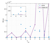
(a) Problem 2

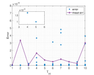
(b) Problem 4 (simplified)

Figure 2: Estimation errors to $Q,R$ without noises. At each $T_{ini}$ we conduct the simulation for $15$ times. The blue scatters represent the estimation error at each experiment. The purple line is the mean error.

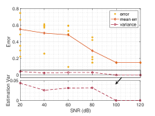
Figure 3: Estimation errors with the presence of observation noises. We conduct the simulation $15$ times for each variance. The orange scatters are errors at each experiment. The solid red curve represents mean of the error and the dashed line for variance.

To demonstrate the computation efficiency, we compare the computation time for the infeasible case between original 3DIOC (Problem 3) and simplified 3DIOC (Problem 5). The results are shown in Table I. We can find that as the initial trajectory length becomes longer, the number of unknown variables in $\lambda_{ini}$ increases and the QP solver consumes more time, while the unknown variables number in simplified 3DIOC only depends on $n,m$, so it remains a constant. The source codes are available at: 3dioc-code.

TABLE I: Computation Time (s)

$T_{ini}$	3	5	7	9	11
Problem 3	1.8102	1.8108	2.9148	4.4705	7.2092
Problem 5	0.6879	0.5949	0.4318	0.5959	0.4381

V conclusion

This paper proposes a direct data-driven IOC algorithm for LQ control problem in LTI systems. With the input-output representation introduced from behavioral system theory, the IOC problem is solved with observation trajectories only. Identifiability condition and perturbation analysis of the estimation are provided. Simulations demonstrate our algorithm achieves a high computation efficiency and requires less data. Note that this 3DIOC framework can also be extended to linear systems with process noises and nonlinear systems utilizing a proper Koopman operator, which will be investigated in our future work.

Appendix A Proof of Theorem 1

From equation (12), we have

$$\mathcal{F}(\lambda_{ini},Q,R)=w_{p}^{T}\operatorname{diag}(\lambda_{ini})\mathbf{1}+2U_{f}^{T}\mathcal{R}\tilde{u}+2Y_{f}^{T}\mathcal{Q}\tilde{y}$$

$$=\begin{pmatrix}w_{p}^{T}&2U_{f}^{T}&2Y_{f}^{T}\end{pmatrix}\begin{pmatrix}\operatorname{diag}(\lambda_{ini})&\\ &\operatorname{diag}(\mathcal{R},\mathcal{Q})\end{pmatrix}\begin{pmatrix}\mathbf{1}\\ \tilde{u}\\ \tilde{y}\end{pmatrix}.$$

Vectorize the function. We have

$$vec(\mathcal{F}(\lambda_{ini},Q,R))=\underbrace{{\begin{pmatrix}\mathbf{1}^{T}&\tilde{u}^{T}&\tilde{y}^{T}\end{pmatrix}\otimes\begin{pmatrix}w_{p}^{T}&2U_{f}^{T}&2Y_{f}^{T}\end{pmatrix}}}_{\Psi}$$ (24)

$$\cdot{vec\begin{pmatrix}\operatorname{diag}(\lambda_{ini})&\\ &\operatorname{diag}(\mathcal{R},\mathcal{Q})\end{pmatrix}}=\Psi\cdot\mathcal{M}(\lambda_{ini},R,Q).$$

The size of matrix $\Psi$ is $[T_{d}-(T_{ini}+N)+1]\times(m+p)^{2}(T_{ini}+N)^{2}$. Since the rank of $\begin{pmatrix}\mathbf{1}^{T}&\tilde{u}^{T}&\tilde{y}^{T}\end{pmatrix}$ is $1$, considering the property of Kronecker product, we have

$$\operatorname{rank}(\Psi)\!=\!rank\begin{pmatrix}w_{p}^{T}&2U_{f}^{T}&2Y_{f}^{T}\end{pmatrix}\!=\!\operatorname{rank}({H}_{T_{ini}+N}(w^{d}))$$

$$=\operatorname{rank}(\mathcal{H}_{T_{ini}+N}(w^{d}))=m(T_{ini}+N)+n.$$

Notice that there are lots of zeros and duplicate items in the vector $\mathcal{M}(\lambda_{ini},R,Q)$. Observing the structure of $\mathcal{M}(\lambda_{ini},R,Q)$ and $\Psi$, we can obtain

$$\Psi\cdot\mathcal{M}(\lambda_{ini},R,Q)$$ (25)

$$=\begin{pmatrix}w_{p}^{T}&\tilde{U}_{f}&\tilde{Y}_{f}\end{pmatrix}\cdot\operatorname{col}(\lambda_{ini},vec(R),vec(Q)),$$

where $\tilde{U}_{f}=\sum_{i=0}^{N-1}\tilde{u}_{i}\otimes 2U_{f}^{T}(im+1:(i+1)m,:)$, $\tilde{Y}_{f}=\sum_{i=0}^{N-1}\tilde{y}_{i}\otimes 2Y_{f}^{T}(ip+1:(i+1)p,:)$. Since weighting matrices $Q,R$ are symmetric, we do further simplification with duplication matrices $D_{m},D_{p}$, which satisfy

$$D_{m}\operatorname{vech}(R)=vec(R),D_{p}\operatorname{vech}(Q)=vec(Q).\vspace{-3pt}$$ (26)

The explicit formula for a duplication matrix for an $m\times m$ matrix is $D_{m}^{T}=\sum_{i\geq j}\tau_{ij}vec(T_{ij})^{T}$, where $\tau_{ij}$ is a unit vector of order $\frac{1}{2}m(m+1)$ having value $1$ in the position $(j-1)m+i-\frac{1}{2}j(j-1)$ and $0$ elsewhere, and $T_{ij}$ is an $m\times m$ matrix with $1$ in position $(i,j),(j,i)$ and $0$ elsewhere.

With these definitions, denote

$$\tilde{\Psi}=\begin{pmatrix}w_{p}^{T}&\tilde{U}_{f}&\tilde{Y}_{f}\end{pmatrix}\cdot\operatorname{diag}(I,D_{m},D_{p})\vspace{-3pt}$$ (27)

We finally have the equation (12) as

$$\Psi\cdot\mathcal{M}(\lambda_{ini},R,Q)=\tilde{\Psi}\cdot\operatorname{col}(\lambda_{ini},\operatorname{vech}(R),\operatorname{vech}(Q))=0\vspace{-3pt}$$ (28)

Matrix $\tilde{\Psi}$ is of order $T-(T_{ini}+N)+1\times(m+p)T_{ini}+\frac{1}{2}(m^{2}+m+p^{2}+p)$. Observing (28), if the rank of $\tilde{\Psi}$

$$\operatorname{rank}(\tilde{\Psi})=(m+p)T_{ini}+\frac{1}{2}(m^{2}+m+p^{2}+p)-1,\vspace{-3pt}$$ (29)

supposing the real weighting matrices are $R,Q$, a solution $(\lambda^{\prime}_{ini},\operatorname{vech}(R^{\prime}),\operatorname{vech}(Q^{\prime}))$ obtained from (28) satisfies $Q=\alpha Q^{\prime},R=\alpha R^{\prime}$ for a scalar $\alpha\in\mathbb{R}_{+}$.

Appendix B Proof of Theorem 2

Considering equation (18), we have

$$\nabla_{u}J(\tilde{u})=:(K_{f}^{T}\mathcal{Q}K_{f}+\mathcal{R})\tilde{u}+K_{f}^{T}\mathcal{Q}^{T}K_{p}z_{ini}$$

$$=\mathcal{R}\tilde{u}+K_{f}^{T}\mathcal{Q}(K_{f}\tilde{u}+K_{p}z_{ini})$$

$$=\underbrace{\begin{pmatrix}K_{f}^{T}&I_{mN}\end{pmatrix}}_{\tilde{K}_{f}}\operatorname{diag}(\mathcal{Q},\mathcal{R})\begin{pmatrix}K_{f}\tilde{u}+K_{p}z_{ini}\\ \tilde{u}\end{pmatrix}=0.$$

$I_{mN}$ represents the identity matrix of $mN\times mN$. Observing (16), we can find that $K_{f}\tilde{u}+K_{p}z_{ini}:=\tilde{y}^{es}$ is actually an estimation to $\tilde{y}$. Through vectorization, we have

$$vec(\nabla_{u}J(\tilde{u}))={\begin{pmatrix}(\tilde{y}^{es})^{T}&(\tilde{u})^{T}\end{pmatrix}\otimes\tilde{K}_{f}}\cdot vec(\operatorname{diag}(\mathcal{Q},\mathcal{R})).$$

Similar to the proof of Theorem 1, we want to eliminate the zeros and duplicate items in $vec(\operatorname{diag}(\mathcal{Q},\mathcal{R}))$. We have

$$vec(\nabla_{u}J(\tilde{u}))=\begin{pmatrix}\Phi_{y}&\Phi_{u}\end{pmatrix}\cdot\operatorname{col}(vec(Q),vec(R)),$$

where $\Phi_{y}=\sum_{i=0}^{N-1}(\tilde{y}^{es}_{i})^{T}\otimes K_{f}^{T}(ip+1:(i+1)p,:)$ and $\Phi_{u}=\sum_{i=0}^{N-1}(\tilde{u}_{i})^{T}\otimes I_{mN}(im+1:(i+1)m,:)$. With duplication matrices $D_{p},D_{m}$ defined in (26), denote

$$\tilde{\Phi}=\begin{pmatrix}\Phi_{y}&\Phi_{u}\end{pmatrix}\operatorname{diag}(D_{p},D_{m})=\begin{pmatrix}\Phi_{y}D_{p}&\Phi_{u}D_{m}\end{pmatrix}.$$ (30)

We finally derive the constraint as

$$vec(\nabla_{u}J(\tilde{u}))=\tilde{\Phi}\cdot\operatorname{col}(\operatorname{vech}(Q),\operatorname{vech}(R))=0.$$ (31)

Observing (31), the unknown variable is only composed by $Q,R$. If there exists a proper $T_{ini}$ making the rank of $\tilde{\Phi}$

$$\operatorname{rank}(\tilde{\Phi})=\frac{1}{2}(m^{2}+m+p^{2}+p)-1,\vspace{-3pt}$$ (32)

supposing the real weighting matrices are $Q,R$, a solution $Q^{\prime},R^{\prime}$ obtained from (31) satisfies $Q=\alpha Q^{\prime},R=\alpha R^{\prime}$ for a scalar $\alpha\in\mathbb{R}_{+}$.

Appendix C Proof of Theorem 3

Suppose the collected online data possesses an uncertainty $\Delta\tilde{u}$, according to the derivation in Appendix B, there is $\Delta\Phi_{y}=\sum_{i=0}^{N-1}(K_{f}\Delta\tilde{u})_{i}^{T}\otimes K_{f}^{T}(ip+1:(i+1)p,:),\Delta\Phi_{u}=\sum_{i=0}^{N-1}(\Delta\tilde{u}_{i})^{T}\otimes I_{mN}(im+1:(i+1)m,:)$. We have

$$\tilde{\Phi}^{\prime} =\underbrace{\begin{pmatrix}\Phi_{y}D_{p}&\Phi_{u}D_{m}\end{pmatrix}}_{\tilde{\Phi}}+\underbrace{\begin{pmatrix}\Delta\Phi_{y}D_{p}&\Delta\Phi_{u}D_{m}\end{pmatrix}}_{\Delta\tilde{\Phi}}.$$

Denote $\Theta(Q,R)=\operatorname{col}(\operatorname{vech}(Q),\operatorname{vech}(R))$. Given the original homogenuos equation $\tilde{\Phi}\cdot\Theta(Q,R)=0$ and the disturbed equation $(\tilde{\Phi}+\Delta\tilde{\Phi})\cdot\Theta(Q^{\prime},R^{\prime})=0$ with the perturbed coefficient matrix, we define the matrix estimation error $\Delta Q=Q-Q^{\prime}$ and $\Delta R=R-R^{\prime}$.

Notice that Problem 5 now is a Rayleigh quotient problem

$$\min_{Q,R}\|\tilde{\Phi}\cdot\Theta(Q,R)\|_{2}^{2}~{}~{}~{}s.t.~{}\|\Theta(Q,R)\|_{2}^{2}=1,\vspace{-3pt}$$

and the optimal solution is the eigenvector of the matrix $\tilde{\Phi}^{T}\tilde{\Phi}$ corresponding to its smallest eigenvalue. We next focus on the deviation between the optimal solutions under $\tilde{\Phi}^{T}\tilde{\Phi}$ and perturbed matrix $(\tilde{\Phi}+\Delta\tilde{\Phi})^{T}(\tilde{\Phi}+\Delta\tilde{\Phi})=\tilde{\Phi}^{T}\Phi+\Delta\tilde{\Phi}^{T}\tilde{\Phi}+\tilde{\Phi}^{T}\Delta\tilde{\Phi}$ (we omit higher order terms here). This can be measured by the eigenvalue perturbation theory [21]. By carrying out the SVD decomposition of matrix

$$\tilde{\Phi}^{T}\tilde{\Phi}=\begin{pmatrix}U&u\end{pmatrix}\operatorname{diag}(\Sigma,\sigma)\operatorname{col}(V^{T},v^{T}),\vspace{-3pt}$$

the smallest eigenvalue is $\sigma$ and the optimal solution $\Theta(Q^{*},R^{*})=v$. According to the eigenvalue perturbation theory, assume $(\sigma^{\prime},v^{\prime})$ are smallest eigenvalue and its corresponding eigenvector to the perturbed matrix and the perturbation $\Delta\Phi$ is much smaller than $\Phi$, we have

$$v^{\prime}-v=\sum_{i=1}^{N_{v}-1}\frac{v_{i}^{T}(\Delta\tilde{\Phi}^{T}\tilde{\Phi}+\tilde{\Phi}^{T}\Delta\tilde{\Phi})v_{i}}{\sigma-\sigma_{i}},\vspace{-3pt}$$ (33)

where $(\sigma_{i},v_{i}),i=1,\dots,N_{v}-1$ are all the other eigenvalues and their corresponding eigenvectors of matrix $\tilde{\Phi}^{T}\tilde{\Phi}$.

References

• [1] N. Ab Azar, A. Shahmansoorian, and M. Davoudi, “From inverse optimal control to inverse reinforcement learning: A historical review,” Annual Reviews in Control, vol. 50, pp. 119–138, 2020.
• [2] H. Ravichandar, A. S. Polydoros, S. Chernova, and A. Billard, “Recent advances in robot learning from demonstration,” Annual Review of Control, Robotics, and Autonomous Systems, vol. 3, pp. 297–330, 2020.
• [3] Y. Xu, J. Xie, T. Zhao, C. Baker, Y. Zhao, and Y. N. Wu, “Energy-based continuous inverse optimal control,” IEEE transactions on neural networks and learning systems, vol. 34, no. 12, pp. 10 563–10 577, 2022.
• [4] J. Mainprice, R. Hayne, and D. Berenson, “Goal set inverse optimal control and iterative replanning for predicting human reaching motions in shared workspaces,” IEEE Transactions on Robotics, vol. 32, no. 4, pp. 897–908, 2016.
• [5] K. Ruan, J. Zhang, X. Di, and E. Bareinboim, “Causal imitation learning via inverse reinforcement learning,” in The Eleventh International Conference on Learning Representations, 2023.
• [6] M. C. Priess, R. Conway, J. Choi, J. M. Popovich, and C. Radcliffe, “Solutions to the inverse lqr problem with application to biological systems analysis,” IEEE Transactions on Control Systems Technology, vol. 23, no. 2, pp. 770–777, 2014.
• [7] Y. Li, Y. Yao, and X. Hu, “Continuous-time inverse quadratic optimal control problem,” Automatica, vol. 117, p. 108977, 2020.
• [8] H. Zhang, J. Umenberger, and X. Hu, “Inverse optimal control for discrete-time finite-horizon linear quadratic regulators,” Automatica, vol. 110, p. 108593, 2019.
• [9] C. Qu, J. He, X. Duan, and S. Wu, “Control input inference of mobile agents under unknown objective,” IFAC-PapersOnLine, vol. 56, 2023.
• [10] W. Jin, T. D. Murphey, D. Kulić, N. Ezer, and S. Mou, “Learning from sparse demonstrations,” IEEE Transactions on Robotics, vol. 39, no. 1, pp. 645–664, 2022.
• [11] S. Byeon, D. Sun, and I. Hwang, “An inverse optimal control approach for learning and reproducing under uncertainties,” IEEE Control Systems Letters, vol. 7, pp. 787–792, 2022.
• [12] W. Xue, P. Kolaric, J. Fan, B. Lian, T. Chai, and F. L. Lewis, “Inverse reinforcement learning in tracking control based on inverse optimal control,” IEEE Transactions on Cybernetics, vol. 52, no. 10, 2021.
• [13] E. Garrabe, H. Jesawada, C. Del Vecchio, and G. Russo, “On convex data-driven inverse optimal control for nonlinear, non-stationary and stochastic systems,” arXiv preprint arXiv:2306.13928, 2023.
• [14] Z. Liang, W. Hao, and S. Mou, “A data-driven approach for inverse optimal control,” in 2023 62nd IEEE Conference on Decision and Control (CDC).   IEEE, 2023, pp. 3632–3637.
• [15] I. Markovsky and F. Dörfler, “Behavioral systems theory in data-driven analysis, signal processing, and control,” Annual Reviews in Control, vol. 52, pp. 42–64, 2021.
• [16] J. C. Willems, P. Rapisarda, I. Markovsky, and B. L. De Moor, “A note on persistency of excitation,” Systems & Control Letters, vol. 54, no. 4, pp. 325–329, 2005.
• [17] I. Markovsky and F. Dörfler, “Identifiability in the behavioral setting,” IEEE Transactions on Automatic Control, vol. 68, pp. 1667–1677, 2022.
• [18] I. Markovsky and P. Rapisarda, “Data-driven simulation and control,” International Journal of Control, vol. 81, no. 12, pp. 1946–1959, 2008.
• [19] J. F. Sturm, “Using sedumi 1.02, a matlab toolbox for optimization over symmetric cones,” Optimization Methods and Software, vol. 11, 1999.
• [20] J. Lofberg, “Yalmip: A toolbox for modeling and optimization in matlab,” in 2004 IEEE International Conference on Robotics and Automation (ICRA).   IEEE, 2004, pp. 284–289.
• [21] F. Rellich, Perturbation theory of eigenvalue problems.   CRC Press, 1969.