Adaptively Coupled Domain Decomposition Method for Multiphase and Multicomponent Porous Media Flows

Abstract

Numerical simulation of large-scale multiphase and multicomponent flow in porous media is a significant field of interest in the petroleum industry. The fully implicit approach is favored in reservoir simulation due to its numerical stability and relaxed constraints on time-step sizes. However, this method requires solving a large nonlinear system at each time step, making the development of efficient and convergent numerical methods crucial for accelerating the nonlinear solvers. In this paper, we present an adaptively coupled subdomain framework based on the domain decomposition method. The solution methods developed within this framework effectively handle strong nonlinearities in global problems by addressing subproblems in the coupled regions. Furthermore, we propose several adaptive coupling strategies and develop a method for leveraging initial guesses to accelerate the solution of nonlinear problems, thereby improving the convergence and parallel performance of nonlinear solvers. A series of numerical experiments validate the effectiveness of the proposed framework. Additionally, by utilizing tens of thousands of processors, we demonstrate the scalability of this approach through a large-scale reservoir simulation with over 2 billion degrees of freedom.

Keywords: Petroleum reservoir simulation, fully implicit method, adaptive domain decomposition method, nonlinear solver, parallel computing.

1.   Introduction

Predicting large-scale multiphase and multicomponent flow processes in porous media is a crucial research field of petroleum reservoir simulation [1, 2, 3]. As the complexity of reservoir development increases and the demand for higher resource utilization efficiency grows, traditional coarse-grid simulation methods have become inadequate for capturing the intricate geological features and fluid dynamics within reservoirs. Modern reservoirs, characterized by high heterogeneity, complex fault systems, and fracture networks, require more refined simulations to accurately predict fluid flow and optimize extraction strategies. However, the higher grid resolution required for refined simulations substantially increases computational costs. At the same time, rapid advancements in computer hardware have provided powerful computational capabilities for increasingly complex reservoir numerical simulations. The prevalence of parallel computing architectures enables researchers to simulate larger-scale models, incorporate more physical processes, and address complex problems within reasonable time frames [4, 5].

In high-resolution reservoir simulation, the fully implicit method (FIM) [6] is one of the most robust approaches for simulating fluid flow in porous media, offering unconditional stability and allowing the relaxation of the Courant-Friedrichs-Lewy (CFL) condition [7]. Using a fully implicit method requires solving a large nonlinear system at each time step. The standard approach to addressing this nonlinearity involves variations of Newton iterations, where a system of linear equations must be solved during each iteration [8]. This process incurs significant computational costs, making it the primary expenses in the simulation [9]. Currently, there is extensive research focused on accelerating the solution of linear systems arising from nonlinear equations in reservoir simulations [10, 11, 12, 13].

Nonlinear preconditioning techniques offer an alternative approach by targeting the elimination of imbalanced nonlinearities within the system. This enhancement improves the global convergence properties of the Newton method, thereby reducing the number of global linear iterations needed. Imbalances in nonlinearity are typically generated by issues such as discontinuities in permeability coefficients, wide variations in fluid properties, strong capillary effects with limited spatial extent, complex source terms, and singularities at corners, faults, or voids. In such situations, the Newton method may encounter slow convergence, resulting in prolonged stagnation or even complete failure to converge [14]. Similar to linear preconditioning, nonlinear preconditioning can be applied to either the left or right side of nonlinear functions. Left nonlinear preconditioners, such as additive Schwarz preconditioned inexact Newton (ASPIN) method [15], multiplicative Schwarz preconditioned inexact Newton (MSPIN) method [16], and restricted additive Schwarz preconditioned exact Newton (RASPEN) method [17], solve nonlinear problems defined on individual subdomains to provide preconditioning for the global nonlinear problem, thereby improving its convergence. In contrast, right nonlinear preconditioners, such as nonlinear elimination (NE) method [18], can be viewed as an inner correction step before the global Newton iterations to precondition areas with stronger nonlinearities in the solution.

ASPIN was first introduced for solving multiphase flow problems in porous media by  [19], demonstrating its potential in addressing challenging problems. [20] tested the robustness of the ASPIN method across various complex scenarios, particularly in fractured reservoirs and three-phase compositional models. They also examined the method’s sensitivity to the pattern of domain decomposition. Additionally, [14] proposed and compared several different NE strategies for two-phase flow problems discretized using the fully implicit discontinuous Galerkin (DG) finite element method. The results demonstrated the superiority of the proposed methods over the classical Newton approach. Furthermore, [21] proposed an adaptive nonlinear preconditioning framework based on convergence monitors, allowing nonlinear preconditioning to be turned off during outer Newton iterations when it is not needed, thereby reducing computational costs while maintaining robustness. In the context of parallel computing, nonlinear preconditioning techniques are closely associated with domain decomposition. For example, in ASPIN, each subproblem is independently defined within a subdomain, meaning the quality of the preconditioner depends on the domain decomposition pattern. In contrast, in NE, a single subproblem may span multiple subdomains, and while these subproblems can often be decoupled into smaller, independent tasks, they are still solved collectively by all processes, potentially reducing computational efficiency. To our knowledge, very limited work has addressed the performance of these nonlinear preconditioning techniques in large-scale reservoir simulations, particularly those with grid sizes exceeding tens of millions. It can be anticipated that as the number of subdomains increases, the performance of the single-level additive Schwarz method (ASM) will inevitably decline rapidly, due to subdomains becoming too small to capture localized features and the neglect of significant couplings between subdomains. On the other hand, for the NE method, the decline in parallel efficiency as the number of processes increases can create difficulties in solving the subproblems collectively with all processes. A potential solution is to dynamically merge the original subdomains into larger subdomains during the simulation and define subproblems within these newly formed larger subdomains, to be collectively solved by all the processes originally assigned to the individual subdomains. This approach not only preserves the important couplings between subdomains but also enhances the ability to capture strong local nonlinearities. An appropriate coupling pattern of subdomains is expected to improve the convergence performance of single-level ASM without significantly compromising parallel efficiency. Furthermore, this approach can provide a foundation for NE to decouple subproblems into multiple independent tasks and solve them separately.

In this paper, we propose a novel framework for adaptively coupled domain decomposition method (ADDM) in the context of large-scale reservoir simulations. The main contributions of this work are listed as follows:

• We develop an efficient framework for subdomain adaptively coupled solutions based on domain decomposition methods to improve both convergence and parallel performance of nonlinear solvers, overcoming the limitations of classic domain decomposition methods.

• We propose several physics-based adaptive coupling strategies and utilize subproblem solutions as initial guesses to accelerate Newton iterations for the global problem.

• The proposed methods are integrated into the open-source simulator OpenCAEPoro [22] for simulating multiphase multicomponent flow in porous media.

• Numerical experiments confirm the convergence and efficiency of this framework. Furthermore, we demonstrate the scalability of this approach by performing a large-scale reservoir simulation with over 2 billion degrees of freedom, utilizing tens of thousands of processors.

The outline of the paper is as follows. Section 2 introduces the mathematical model for multiphase and multicomponent flows in porous media, followed by the corresponding fully implicit discretization. In Section 3, we present in detail a framework for subdomain adaptively coupled decomposition methods, which serves as a key component of the nonlinear solver. In Section 4, numerical experiments are conducted to assess the effectiveness and parallel performance of the proposed framework. Finally, Section 5 summarizes the work presented in this paper.

2.   Mathematical Model and Discretization Method

This section will review the governing equations and discretization methods used for the multiphase and multicomponent model in porous media.

2.1 Mathematical model

We consider an isothermal multicomponent model that includes $n_{c}$ components and $n_{p}$ phases [2]. The mass conservation equations for component $i$ is

$$\frac{\partial}{\partial t}{N_{i}}+\nabla\cdot\sum_{j=1}^{n_{p}}\left(x_{ij}\xi_{j}\mathbf{u}_{j}-\xi_{j}\mathbf{D}_{ij}\nabla x_{ij}\right)=Q_{i},\quad i=1,\ldots,n_{c},$$ (1)

where $N_{i}$ is molar concentration of component $i$, $x_{ij}$ is mole fraction of component $i$ in phase $j$, $\xi_{j}$ is molar density of phase $j$, $\mathbf{u}_{j}$ is volumetric flow rate of phase $j$, and $\mathbf{D}_{ij}$ is diffusion coefficient tensor of component $i$ in phase $j$. $Q_{i}$ is volumetric molar injection or production rate for component $i$. Wells are described using a standard Peaceman type well model [23].

Based on Darcy’s Law, we have

$$\mathbf{u}_{j}=-\frac{\boldsymbol{\kappa}\kappa_{rj}}{\mu_{j}}(\nabla P_{j}-\rho_{j}g\nabla z),\quad j=1,\ldots,n_{p},$$ (2)

where $\boldsymbol{\kappa}$ is effective permeability of rock, $\kappa_{rj}$ is relative permeability of phase $j$, $\mu_{j}$ is mass density of phase $j$, $P_{j}$ is pressure of phase $j$, $\rho_{j}$ is mass density of phase $j$, and $z$ is depth.

Additionally, some constraints should be added among these physical quantities.

• Saturation constraint equation:

  $$\sum_{j=1}^{n_{p}}S_{j}=1.$$ (3)

• Molar fraction constraint equation:

  $$\sum_{i=1}^{n_{c}}x_{ij}=1,\leavevmode\nobreak\ j=1,\ldots,n_{p}.$$ (4)

• Capillary pressure equation:

  $$P_{j}=P-P_{cj},\leavevmode\nobreak\ j=1,\ldots,n_{p},$$ (5)

  where $P$ is pressure of reference phase, and $P_{cj}$ is capillary pressure between the reference phase and phase $j$.

• Volume constraint equation:

  $$V_{f}=V_{p},$$ (6)

  where $V_{f}$ is fluid volume and $V_{p}$ is pore volume.

It is important to note that the above system of equations is general, with different model equations being implicitly embedded within the relationships between the variables. For instance, when the classic black oil model is employed, phase saturation $S_{j}$, the molar fraction of components in phases $x_{ij}$, and molar density $\xi_{j}$ are explicitly obtained from pressure $P$ and the molar density of components $N_{i}$. In contrast, for compositional models, complex phase equilibrium calculations are required. Besides, fluid permeability properties, rock compressibility properties, convection-diffusion characteristics of phases and components, as well as well behaviors, can be described by various models.

2.2 Discretization method

The equations are discretized in space using a finite-volume scheme with a two-point flux approximation and upwind weighting [24, 25], and in time using an implicit (backward) Euler scheme. In each grid cell, we have

$$F_{v}\coloneqq V_{p}^{(n+1)}-V_{f}^{(n+1)} =0,$$ (7)

$$F_{n_{i}}\coloneqq\frac{N_{i}^{(n+1)}-N_{i}^{(n)}}{{\delta t}^{(n+1)}}+\sum\limits_{s}\sum_{j=1}^{n_{p}}\left[T_{s,ij}^{(n+1)}\left(\Delta P_{j}^{(n+1)}-\rho_{j}^{(n+1)}g\Delta z\right)\right]_{s}+Q_{i}^{(n+1)} =0,$$ (8)

$$i=1,\ldots,n_{c},$$

where $s$ represents the interface between the grid cell and its neighboring cell, and the operator $\Delta$ denotes the difference in the corresponding variable between the two grid cells on either side of the interface. $T_{s,ij}$ represents the transmissibility of component $i$ in phase $j$ across surface $s$. For detailed information on discretization, we recommend readers refer to [2, 26]

The above nonlinear system is then solved simultaneously using a fully implicit formulation with a Newton-type method. In our approach, the primary variables are chosen as $P,N_{1},\dots,N_{n_{c}}$. The Newton search direction is

$$\boldsymbol{d}=-\boldsymbol{J}^{-1}\boldsymbol{F},$$ (9)

where $\boldsymbol{F}$ represents the residual, and $\boldsymbol{J}$ is the Jacobian matrix.

3.   Adaptively Coupled Domain Decomposition Method

In this section, we first introduced the motivation for this research, explaining its significance and practical applications in solving large-scale complex problems. Next, we presented three adaptive coupling strategies for subdomains and discussed their advantages and disadvantages. Finally, we provided the method for setting boundary conditions for the subdomains, as well as the solution framework of the adaptively coupled domain decomposition method.

3.1 The Proposed Method

Domain decomposition methods (DDM) are inherently parallel computing techniques that partition the entire computational domain into multiple subdomains, each of which is handled by one or more processes. Nonlinear preconditioning techniques are often parallelized using DDM as well. For example, in the ASPIN method, each subproblem is independently defined within a subdomain, meaning that the quality of the preconditioner depends on how the domain is decomposed. It is foreseeable that as the number of subdomains increases (and their size decreases), the performance of the single-level ASM will inevitably decline rapidly. This is because the subdomains become too small to effectively capture local features, while important coupling relationships between subdomains are neglected. In this case, increasing the overlap between subdomains or designing more appropriate transmission conditions offers only limited improvements. Adopting a two-level strategy can effectively enhance convergence [27]; however, constructing an efficient coarse grid problem remains highly challenging. In large-scale, fine-grid simulations, even the coarse grid problem can be quite large, facing difficulties similar to those of the original problem. Moreover, efficiently implementing multilevel algorithms is also a significant challenge, often requiring substantial modifications to existing code.

A feasible solution is to dynamically merge existing subdomains into larger subdomains during the simulation and define subproblems within these newly formed, larger subdomains. These subproblems are then solved collaboratively by all the processes originally responsible for the smaller subdomains. This approach not only preserves important coupling relationships between subdomains but also better captures strong local nonlinear characteristics. We refer to this as the adaptively coupled domain decomposition method (ADDM). This method is expected to enhance the convergence of single-level ASM while maintaining parallel efficiency. The strategy of dynamically coupling subdomains for solving during the reservoir simulation is based on three fundamental observations:

1. Effectively addressing strong local nonlinearities in the global problem is key to improving convergence performance.

2. Regions with strong nonlinearities (e.g., the advancing fluid fronts near wells when they begin operation) are typically localized, occupying relatively small areas within the entire computational domain, and these regions change dynamically throughout the simulation.

3. Most linear and nonlinear solving algorithms can sustain high parallel efficiency when using a small number of processes.

Therefore, if the simulation can accurately identify those strongly nonlinear regions that cause convergence difficulties and couple the relevant subdomains to define subproblems on them, then the solutions of these subproblems will better approximate the local solutions of the global problem. Using these solutions as preconditioners or initial guesses for the global problem can significantly improve convergence. Furthermore, since each coupled region remains relatively small compared to the overall computational domain, solving them can maintain high computational efficiency.

Figure 1 illustrates the subdomain adaptive coupling strategy. The computational domain is a square with four gas injection wells located at the corners and a production well at the center. This domain is divided into 784 subdomains, each managed by a single process, as shown in Figure 1(a). Figure 1(b) displays the gas phase saturation distribution at a specific time, while Figure 1(c) shows the absolute value of the change in gas phase saturation from the previous time step. The figures reveal that fluid flow is highly intense near the gas front, demonstrating strong nonlinear behavior, whereas regions farther from the front exhibit smoother flow with significantly reduced nonlinearity. In Figure 1(d), all subdomains are categorized into five types. Subdomains marked with the lightest color (value -1) have their subproblems solved independently. For other types, subdomains marked with the same color are coupled into larger regions, and the subproblems defined on these larger regions are solved collectively by the processes initially responsible for these subdomains. Additionally, Figures 1(c) and 1(d) show that the moving front region is relatively small compared to the entire computational domain. Consequently, the number of subdomains requiring coupling for solving remains manageable.

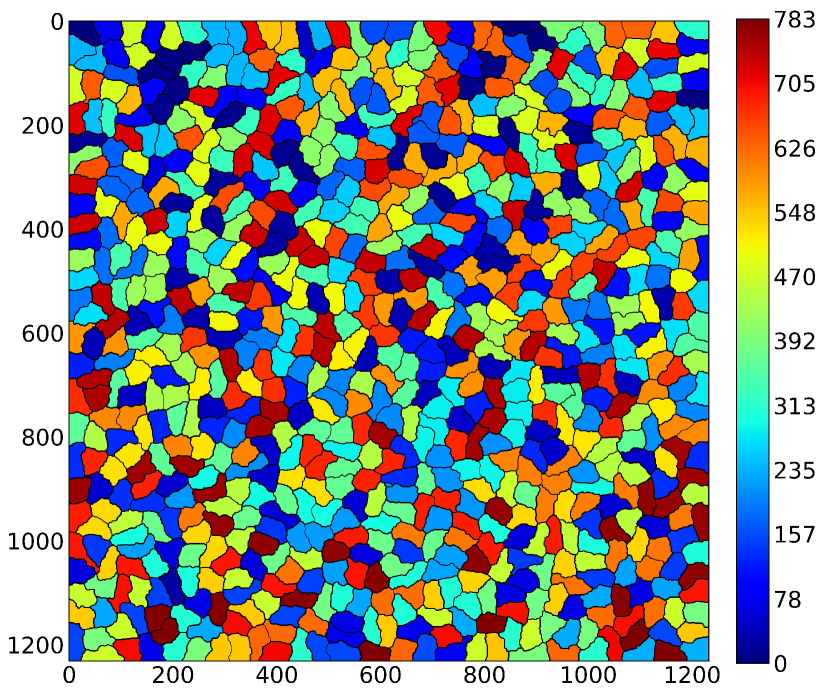
(a)

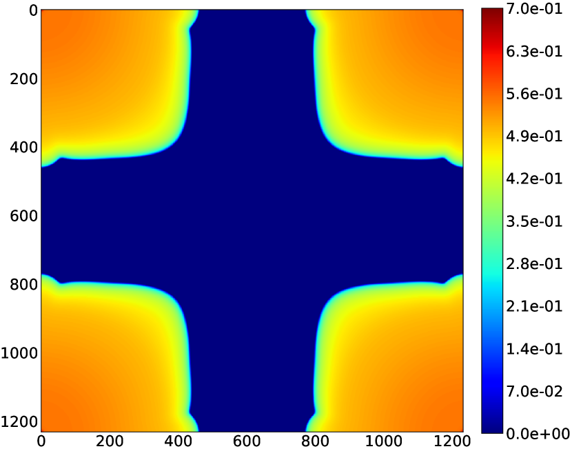
(b)

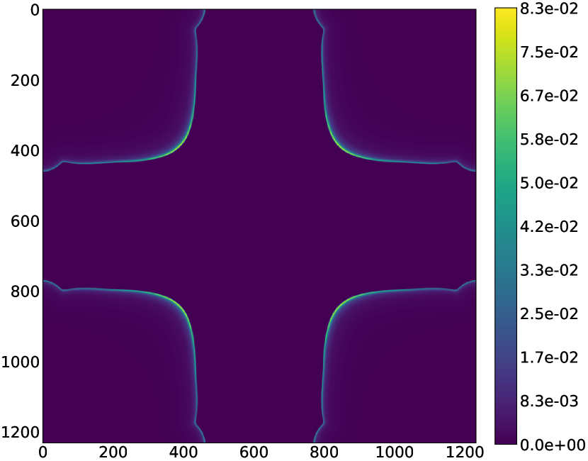
(c)

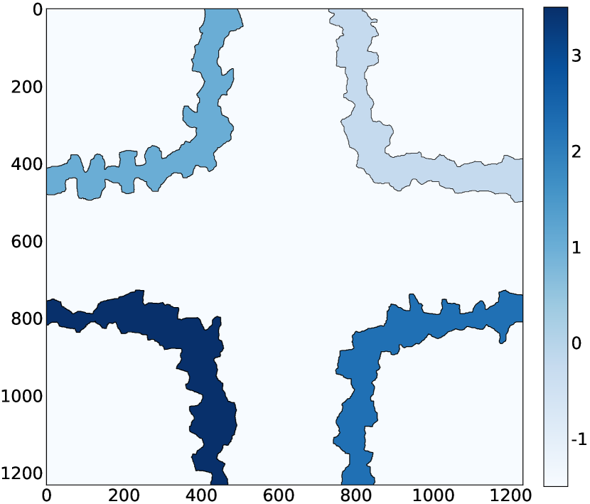
(d)

Figure 1: Illustration of the adaptive subdomain coupling solution: (a) Subdomain partitioning pattern, (b) Gas phase saturation distribution, (c) Gas phase saturation variation, (d) Subdomain coupling pattern.

In underground oil recovery processes, one fluid phase typically displaces another, and strong nonlinear characteristics are often present at the moving front of the fluid. By monitoring changes in saturation within the reservoir, we can effectively capture the position of the displacement front. Coupling subdomains essentially involves classifying them, a process that can be achieved through graph partitioning based on their connectivity graph. Therefore, there are two main challenges: first, how to construct the connectivity graph between subdomains; and second, how to effectively partition the resulting graph.

Next, we will delve into the discussion of the two key issues mentioned above. Before proceeding, let’s assume that the entire computational domain $\Omega$ is divided into $N$ subdomains, denoted as $\Omega_{i}$, such that ${\Omega}=\bigcup_{i=1}^{N}{\Omega}_{i}$ and $\Omega_{i}\cap\Omega_{j}=\emptyset$ for all $i\neq j$. We now define an undirected graph $G(\Omega)$ where each vertex represents a subdomain $\Omega_{i}$, and the edges are defined based on the relationships between subdomains, specifically the strength of coupling between them. To identify the advancing front, we first locate the regions with significant changes in saturation. Specifically, we identify the grid cells within each subdomain where the saturation change exceeds a specified threshold $c_{{}_{S}}$ (a positive number), which is defined as follows:

$$M_{k,l}=\left\{i\mid\exists\,j\;\text{s.t.}\;|\Delta S_{j,i}^{(n)}|>c_{{}_{S}},\,j=1,\dots,n_{p},\,i\in\Omega_{k,l}\right\},$$

where $\Omega_{k,l}$ is the set of subdomains obtained by expanding $\Omega_{k}$ outward by $l$ layers. Hence, we have $\Omega_{k}=\Omega_{k,0}$, and let $M_{k}=M_{k,0}$. Figure 2 illustrates an example where the computational domain is divided into $4\times 4$ subdomains. The blue curve marks the grid cells identified by the saturation change threshold, and this curve spans multiple subdomains.

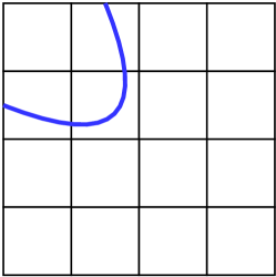
Figure 2: Subdomain partitioning and displacement front.

We have proposed three strategies for adaptive coupling of subdomains:

1. Based on saturation changes at subdomain boundaries (ADDM01): For adjacent subdomains $\Omega_{i}$ and $\Omega_{j}$, if there are grid cells with saturation changes greater than a specified threshold near their boundary, then $\Omega_{i}$ and $\Omega_{j}$ are coupled. This is expressed as

   $$E(\Omega_{i},\Omega_{j})\in G({\Omega}),\quad\text{if and only if}\quad M_{i,l}\cap M_{j,l}\neq\emptyset.$$

   The coupling pattern is obtained by calculating the connected components of the graph $G({\Omega})$. Figure 3 shows an example for $l=1$, where green subdomains are coupled for solving and gray subdomains are solved independently. This strategy focuses on identifying important couplings between subdomains to precisely capture the driving front with a few subdomains.

   

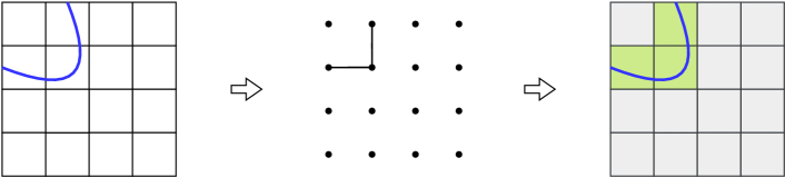
   Figure 3: Illustration of the first subdomain coupling strategy.

2. Based on active subdomains (ADDM02): For a subdomain $\Omega_{i}$ where saturation changes exceed the specified threshold, $\Omega_{i}$ is considered active, and all its neighboring subdomains are coupled, expressed as

   $$E(\Omega_{i},\Omega_{j})\in G({\Omega}),\;\text{for all neighboring subdomains }\,\Omega_{j},\quad\text{if }M_{i}\neq\emptyset.$$

   The coupling pattern is determined by calculating the connected components of the graph $G({\Omega})$. Figure 4 illustrates this strategy, where green subdomains are coupled for solving and gray subdomains are solved independently. This approach considers both important couplings and the movement of the advancing front, increasing robustness but also leading to a larger number of coupled subdomains. Clearly, the coupled subdomains in the first strategy form a subset of those in the second strategy.

   

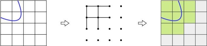
   Figure 4: Illustration of the second subdomain coupling strategy.

3. Based on weighted graph of subdomains (ADDM03): For adjacent subdomains $\Omega_{i}$ and $\Omega_{j}$, define their connection weight as

   $$W(\Omega_{i},\Omega_{j})=\left(\sum_{k\in M_{i}}+\sum_{k\in M_{j}}+\sum_{k\in M_{i,l}\cap M_{j,l}}\right)\sum_{j=1}^{n_{p}}\left|\Delta S_{j,k}\right|,\quad\text{for }M_{i,1}\cap M_{j,1}\neq\emptyset,$$

   which takes into account both its own activity and the coupling strength with its neighbors. If $W(\Omega_{i},\Omega_{j})=0$, a very small value is assigned to represent the connection between the two subdomains. The weighted graph $G(\Omega)$ is partitioned into a specified number of blocks, as shown in Figure 5. Subdomains marked with the same color are coupled for solving. This strategy provides a comprehensive consideration of couplings between subdomains, effectively utilizing parallel computing resources by coupling as many subdomain partitions as possible in a partition-wise manner. Additionally, it can prevent the formation of excessively large coupled subdomains by maintaining a controlled number of partitions. However, it is less flexible in capturing irregular shapes and sacrifices some recognition capability in critical regions.

   

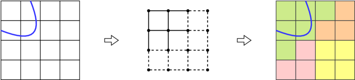
   Figure 5: Illustration of the third subdomain coupling strategy.

For ADDM01 and ADDM03, the value of $l$ is typically chosen as 1 or 2. Regarding the saturation change threshold $c_{{}_{S}}$, we propose several heuristic selection strategies:

1. $c_{{}_{S}}=5\times 10^{-3}$.

2. $c_{{}_{S}}=1\times 10^{-3}$.

3. $c_{{}_{S}}=1\times 10^{-3}\times\dfrac{\delta t^{(n)}}{\delta t_{\text{max}}}$, where $\delta t_{\text{max}}$ is a preset optional maximum time step.

4. $c_{{}_{S}}=1\times 10^{-3}\times\dfrac{\delta t^{(n)}}{\delta t^{(n+1)}}$, where $\delta t^{(n)}$ and $\delta t^{(n+1)}$ are the previous and current time steps, respectively.

Strategies (A) and (B) use fixed thresholds. When the time step is small, saturation changes are generally minor and may not reach the specified threshold, allowing all subdomains to be solved independently. This is reasonable to some extent, as a smaller time step typically corresponds to reduced nonlinearity, reducing or eliminating the need for extra computational resources for nonlinear preconditioning or initial solution preprocessing. Strategies (C) and (D) implement dynamic thresholding, taking into account the influence of time step size, which makes them more robust. Strategy (C) focuses on the rate of saturation change

$$\frac{\left|\Delta S^{(n)}\right|}{\delta t^{(n)}}>\frac{1\times 10^{-3}}{\delta t_{\text{max}}}.$$

Strategy (D) considers changes in the time step size, with the threshold decreasing as the next time step increases, and increasing as the time step decreases. This approach ensures that the number of coupled subdomains is generally positively correlated with the time step length.

The Boost Graph Library (BGL) toolset [28] can be used to compute the connected components of a graph. BGL is a highly efficient C++ library tailored for graph-related problems, offering a comprehensive range of data structures and algorithms, including graph traversal, shortest path computation, minimum spanning tree construction, and connected components identification. For partitioning weighted graphs, the Metis toolset [29] is well-suited. Metis is a robust and efficient library specifically designed for partitioning large-scale graphs, offering advanced algorithms that enable rapid multilevel graph partitioning.

It is important to note that the computational cost of subdomain coupling partitioning is typically very low because its complexity is related to the initial number of subdomains, $N$, which is usually small. Additionally, due to the localized nonlinear distribution characteristics of the problem, most subdomains can be independently solved in practice. In the first two coupling strategies, these subdomains are excluded before graph partitioning, while in the third strategy, the independently solved subdomains contribute a large number of low-weight edges, which connect them to neighboring subdomains. Therefore, their computational cost is almost negligible.

3.2 Subdomain Boundary Conditions

After completing the adaptive coupling of subdomains, the overall system retains a domain decomposition structure. The key difference is that some regions consist of multiple smaller, coupled subdomains, which are jointly managed by the corresponding processes. At this stage, boundary conditions for non-coupled neighboring regions must be addressed, similar to classical domain decomposition methods. Typically, the boundary conditions between subdomains are determined based on information from these non-coupled neighboring regions in the previous iteration step. A common approach is to apply Dirichlet boundary conditions for pressure or component flow rates. Furthermore, the flux across boundaries is calculated using the upstream weighting principle.

3.3 The Solving Framework of ADDM

In this section, we propose an adaptively coupled domain decomposition method solution framework. Without loss of generality, we assume that at time $t$, the domain decomposition after coupling is defined as ${\Omega}=\bigcup_{i=1}^{{N}^{t}}{\Omega}_{i}^{t}$, where ${\Omega}_{i}^{t}\cap{\Omega}_{j}^{t}=\emptyset$ (for $\forall\leavevmode\nobreak\ i\neq j$). Here, ${\Omega}_{i}^{t}=\bigcup_{j\in\mathcal{N}_{i}^{t}}\Omega_{j}$, where $\mathcal{N}_{i}^{t}$ is the index set of the subdomains that form ${\Omega}_{i}^{t}$, satisfying $\bigcup_{i=1}^{N^{t}}\mathcal{N}_{i}^{t}=\left\{1,2,\dots,N\right\}$ and $\mathcal{N}_{i}^{t}\cap\mathcal{N}_{j}^{t}=\emptyset$ (for $\forall\leavevmode\nobreak\ i\neq j$). At time $t$, if all subdomains are coupled and solved together, the method results in a fully coupled algorithm with ${N}^{t}=1$ and ${\Omega}_{1}^{t}=\Omega$. On the other hand, if each subdomain is solved independently, the method reverts to the classical domain decomposition method (CDDM) with ${N}^{t}=N$ and ${\Omega}_{i}^{t}=\Omega_{i}$.

As a solution framework, the key aspect of this method lies in identifying important subdomain coupling relationships during the simulation. After the subdomains are coupled, the system still maintains a domain decomposition structure. Therefore, strategies from classical domain decomposition methods, such as overlapping subdomains and multilevel domain decomposition [27], are also applicable to this framework. Methods that already utilize domain decomposition strategies can enhance algorithmic convergence performance by replacing their domain decomposition components with subdomain adaptive coupling strategies. For example, in the classical ASPIN algorithm, the original domain decomposition structure $\left\{\Omega_{i}\right\}_{i=1}^{N}$ can be replaced by $\left\{{\Omega}_{i}^{t}\right\}_{i=1}^{{N}^{t}}$ while keeping the remaining algorithm steps unchanged. Similarly, in the NE algorithm, the entire computational domain can be repartitioned using the subdomain adaptive coupling method, followed by the identification and solution of strongly nonlinear parts within each ${\Omega}_{i}^{t}$, to correct the global solution.

We propose an algorithm within the subdomain adaptive coupling solution framework, where the solution to the local nonlinear problem defined on ${\Omega}_{i}^{t}$ is used as the initial guess for the global nonlinear problem. As an example, we employ the FIM formulation combined with a Newton-type method to solve both local and global nonlinear problems, with convergence residual thresholds $\epsilon_{\text{local}}$ and $\epsilon_{\text{global}}$, respectively. Given an initial guess $\mathbf{X}^{(1)}$, and the current approximate solution $\mathbf{X}^{(n)}$ at time $t^{n}$, the new approximate solution $\mathbf{X}^{(n+1)}$ can be computed using the following steps:

1

Input: $\mathbf{X}^{(n)}$, $\{{\Omega}_{i}\}_{i=1}^{N}$, $\epsilon_{\text{local}}$, $\epsilon_{\text{global}}$, $MaxIt$;

2

3Determine $\left\{{\Omega}_{i}^{t}\right\}_{i=1}^{{N}^{t}}$ using adaptive coupling strategies (see Section 3.1);

4Set $\mathbf{X}_{i}^{1}=\left.\mathbf{X}^{(n)}\right|_{{\Omega}_{i}^{t}}$, for $\forall\leavevmode\nobreak\ i=1,\ldots,N^{t}$;

5for $k=1,\ldots,MaxIt$ do // Solve local nonlinear problem $\mathcal{F}_{i}(\mathbf{X})=0$ with initial guess $\mathbf{X}_{i}^{1}$

6       Parallel for $i=1,\ldots,N^{t}$ do // Solve subproblems in parallel

7             Compute local Jacobian matrix $\mathbf{J}_{i}=\mathcal{F}^{\prime}_{i}(\mathbf{X}_{i}^{k})$;

8            Solve local linear system $\mathbf{J}_{i}\mathbf{d}_{i}=-\mathbf{F}_{i}$;

9            Compute local step size $\alpha_{i}$ obtained by backtracking line search;

10            Update $\mathbf{X}_{i}^{k+1}=\mathbf{X}_{i}^{k}+\alpha_{i}\mathbf{d}_{i}$;

11            if $\|\mathcal{F}_{i}(\mathbf{X}_{i}^{k+1})\|\leq\epsilon_{\text{local}}\|\mathcal{F}_{i}(\mathbf{X}_{i}^{1})\|$ then break;

12            

13       end for

14      

15 end for

16

17Set $\left.\mathbf{\bar{X}}^{1}\right|_{{\Omega}_{i}^{t}}=\mathbf{X}_{i}^{k+1}$, for $\forall\leavevmode\nobreak\ i=1,\ldots,N^{t}$;

18for $k=1,\ldots,MaxIt$ do // Solve global nonlinear problem $\mathcal{F}(\mathbf{X})=0$ with initial guess $\mathbf{\bar{X}}^{1}$

19       Compute global Jacobian matrix $\mathbf{J}=\mathcal{F}^{\prime}(\mathbf{\bar{X}}^{k})$;

20      Solve global linear system $\mathbf{J}\mathbf{d}=-\mathbf{F}$;

21      Compute global step size $\alpha$ obtained by backtracking line search;

22      Update $\mathbf{\bar{X}}^{k+1}=\mathbf{\bar{X}}^{k}+\alpha\mathbf{d}$;

23      if $\|\mathcal{F}(\mathbf{\bar{X}}^{k+1})\|\leq\epsilon_{\text{global}}\|\mathcal{F}(\mathbf{\bar{X}}^{1})\|$ then break;

24      

25 end for

26

27Set $\mathbf{X}^{(n+1)}=\mathbf{\bar{X}}^{k+1}$;

Output: $\mathbf{X}^{(n+1)}$.

Algorithm 1 ADDM Solution Framework — Initial Guess for Nonlinear Problems

4.   Numerical experiments

In this section, we present numerical results from a series of experiments designed to evaluate the convergence and parallel performance of the newly proposed adaptively coupled domain decomposition method (ADDM). The experiments focus on three key aspects: a comprehensive analysis and discussion of adaptive coupling strategies, an investigation of ADDM’s applicability to complex heterogeneous problems, and a weak scaling study of ADDM. We compared three solution methods, which are respectively denoted as:

1. FIM: Directly solving the global nonlinear problem using a fully implicit method.

2. CDDM: Algorithm 1 without adaptive coupling strategies, where subproblems are defined on the original subdomains.

3. ADDM*: Algorithm 1 with a series of adaptive coupling strategies.

Typically, the choice of time steps is critical to the performance of solution methods. However, in practice, devising an optimal strategy is often challenging. Therefore, to facilitate method comparison and enhance the significance of our experimental results, we adopted the following approach: multiple experiments were conducted to select optimal time steps for FIM, and the same configuration was then applied to all other methods.

In this work, the proposed method is implemented in our open-source parallel reservoir simulator, OpenCAEPoro [22]. For linear solvers, we used the constrained pressure residual (CPR) preconditioned iterative method [30, 31], implemented with the portable, extensible toolkit for scientific computation (PETSc) [32] and Hypre [33, 34, 35] libraries. In the CPR preconditioner, the first stage employs Hypre’s Boomer-AMG to solve the pressure subsystem, while the second stage uses PETSc’s Block-Jacobi with ILU(0) to solve the overall system. Additionally, the iterative method employed is the flexible generalized minimal residual method (FGMRES) [36]. The relative residual norm tolerance is set to $\epsilon_{\text{global}}=10^{-4}$ for both the global nonlinear and linear problems, and to $\epsilon_{\text{local}}=10^{-2}$ for the local nonlinear and linear problems, with a maximum of 100 iterations allowed. Finally, numerical experiments are conducted on a supercomputer equipped with two Intel 6458Q CPUs, each featuring 32 cores operating at 3.1 GHz, and 256 GB of local memory per compute node.

4.1 Case 1

We use this example to conduct a comprehensive analysis and discussion on adaptive coupling strategies. This case is based on the extension and reconstruction of the SPE1 benchmark [37]. Specifically, we refined the original model to a certain scale, then extended the grid horizontally. Additionally, we modified the well pattern to four injection wells and one production well, with injection wells located at the four corners and the production well at the center. The perforation layers remain consistent with the original benchmark. Finally, we constructed an initial model with a grid size of $1232\times 1232\times 10$, where each grid cell measures $20\text{ft}\times 20\text{ft}\times 10\text{ft}$. The injection wells are operated at a gas injection rate of $20000\text{Mscf/day}$, with perforations in the top two layers. The production well is maintained at an oil production rate of $20000\text{stb/day}$, with perforations in the bottom five layers.

4.1.1 Initial model

We simulated a total period of 5000 days using 784 processes. Figure 6 illustrates the spatial distribution of gas saturation in the first layer of the reservoir at various time points. The entire flow process can be broadly divided into three stages: before gas convergence, during gas convergence, and after gas breakthrough to the production well. At different stages, the characteristics and complexity of problems vary, thereby providing a more comprehensive reflection of the performance of various methods.

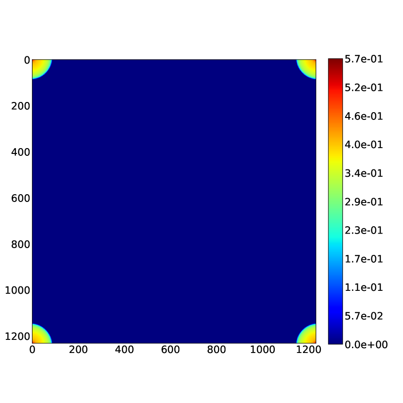
(a) The 60th day

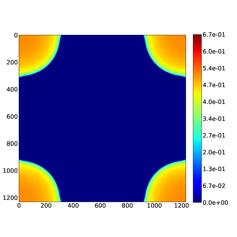
(b) The 750th day

(c) The 2000th day

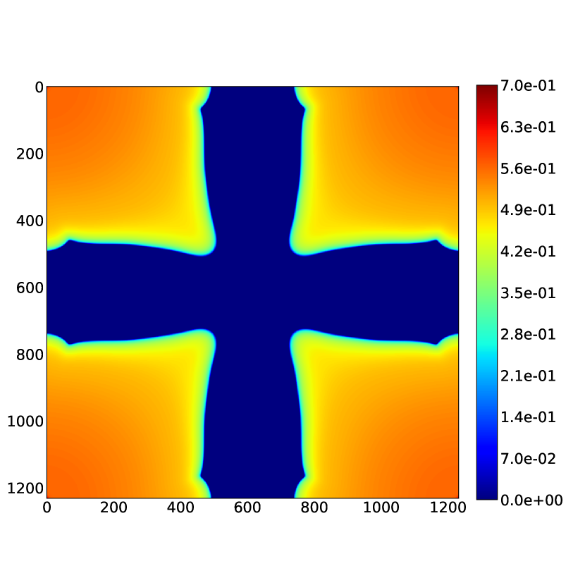
(d) The 2600th day

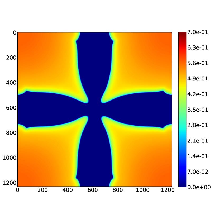
(e) The 2820th day

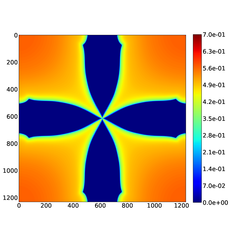
(f) The 3000th day

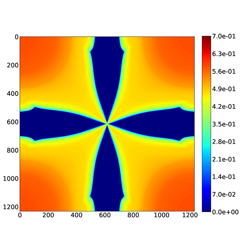
(g) The 4000th day

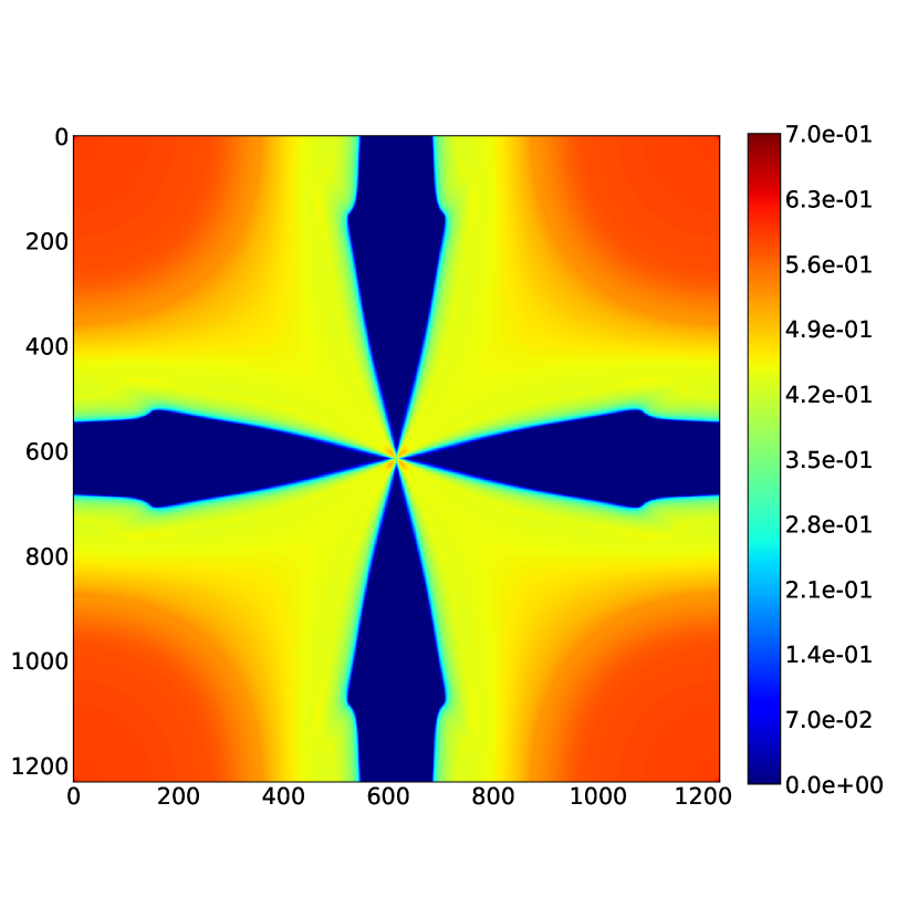
(h) The 5000th day

Figure 6: The gas saturation in the first layer of the reservoir at different time points.

Figure 7(a) presents the result of domain partitioning. It is important to note that, due to the significantly larger number of grid cells in the horizontal direction compared to the vertical direction, the grid partitioning achieved using ParMetis [38] is effectively two-dimensional. Moreover, Figures 7(b), 7(c), and 7(d) also illustrate these three stages from another perspective and verifies the consistency of the computational results across the FIM, CDDM, ADDM01, ADDM02, and ADDM03 methods, where the suffixes 01, 02, and 03 represent different subdomain coupling patterns. Unless otherwise specified, $c_{s}$ is chosen as $5\times 10^{-3}$, which corresponds to Strategy A (see Section 3.1). The boundary condition is set to a constant pressure condition (see Section 3.2). We observe that the average field pressure continuously rises initially and then decreases after breakthrough; the gas production rate remains constant at first and then rapidly increases after breakthrough. Combining Figures 6 and 7, we can infer that the gas from the four injection wells converged and subsequently broke through to the production well between days 2820 and 3000.

(a)

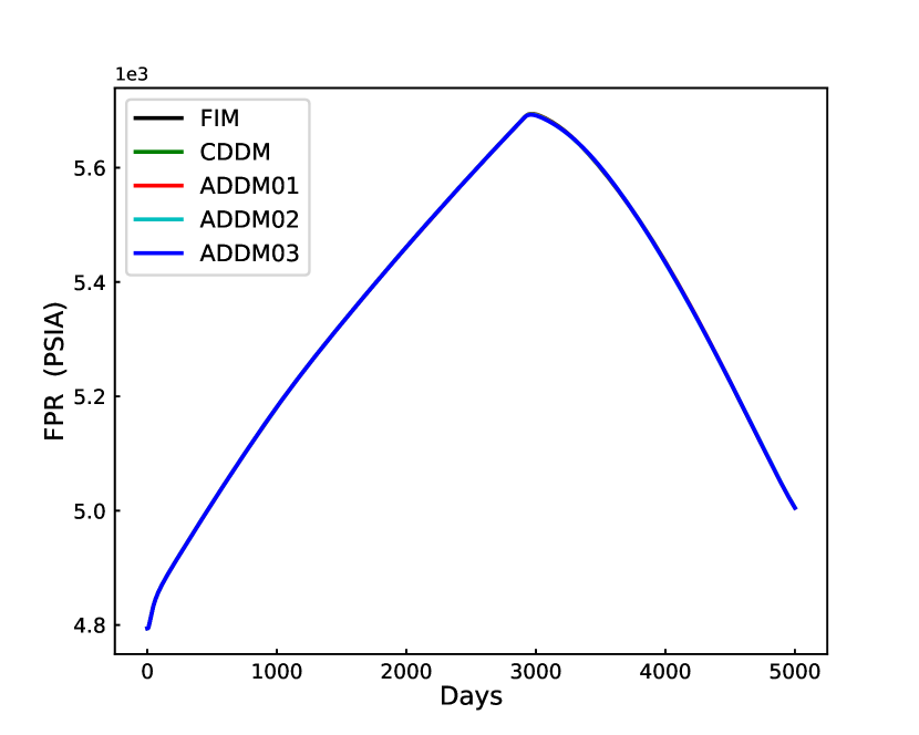
(b)

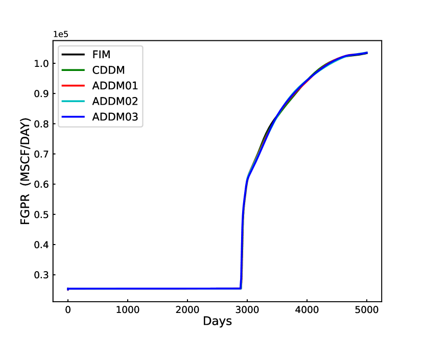
(c)

(d)

Figure 7: Figure (a) displays the domain partitioning by 784 processes using ParMetis, with colors corresponding to the rank of each process. Figures (b), (c), and (d) shows the field average pressure (FPR), field gas production rate (FGPR) and field water production rate (FWPR), respectively, which verify the consistency of the results obtained by the five methods.

The motivation for using (A/C)DDM methods to provide initial solutions for global solution methods (e.g., FIM) is to reduce the number of Newton-Raphson iterations (NRiter) required for solving global nonlinear problems, thereby decreasing the number of iterations needed by the global linear solver (LSiter) . As illustrated in Figure 8(b) and Figure 8(c), compared to FIM, all (A/C)DDM methods exhibit a substantial decrease in NRiter and, consequently, in LSiter. For example, CDDM reduced NRiter by $19.7\%$ on the 3000th day and by $13.7\%$ on the 5000th day, while reducing LSiter by $23.6\%$ on the 3000th day and by $15.8\%$ on the 5000th day. Similarly, ADDM02 reduced NRiter by $52.3\%$ on the 3000th day and by $40.7\%$ on the 5000th day, while reducing LSiter by $57.8\%$ on the 3000th day and by $37.0\%$ on the 5000th day. This indicates that using (A/C)DDM can effectively enhance the convergence performance of global problems in most time, thereby reducing the required NRiter and LSiter. Specifically, the (A/C)DDM methods also exhibit a significant advantage in terms of LS/NR, particularly during the first 3000 days, as shown in Figure 8(d).

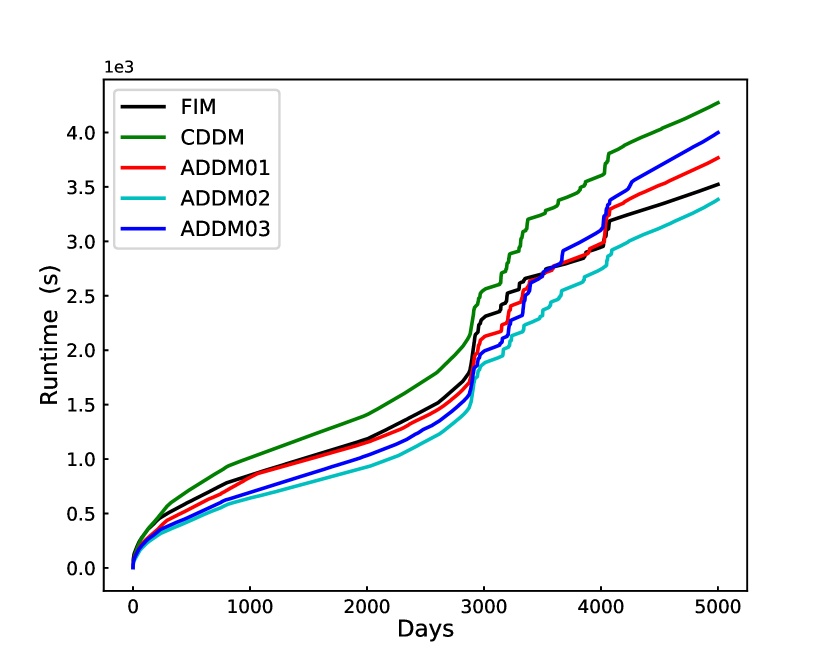
(a)

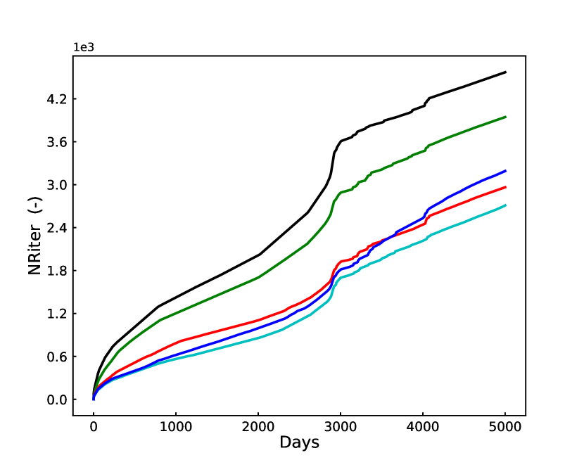
(b)

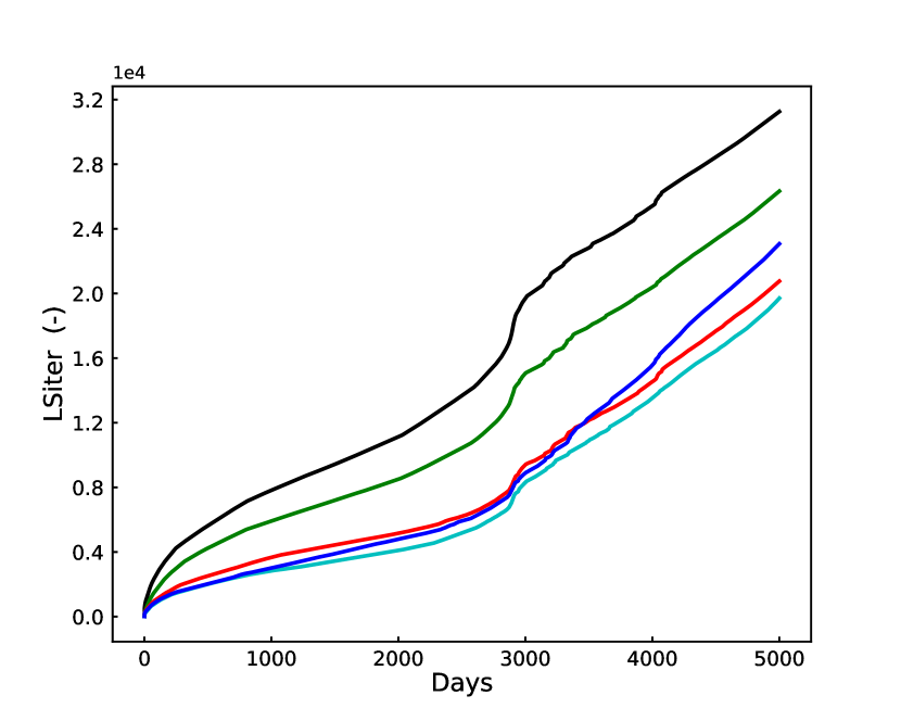
(c)

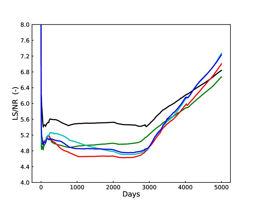
(d)

Figure 8: Figures (a), (b), (c), and (d) illustrate the performance of these methods from four perspectives: wall time from the first time step to the last time step (Runtime), cumulative global Newton-Raphson iterations (NRiter), cumulative global linear iterations (LSiter), and the ratio of LSiter to NRiter (LS/NR).

While the reduction in NRiter and LSiter offers clear advantages, it incurs an additional cost—solving a large number of smaller subproblems. In some cases, this overhead may not fully compensate for the benefits gained. Table 1 presents a more detailed runtime comparison. It can be observed that although CDDM significantly reduces NRiter and LSiter compared to FIM, it is almost always slower than FIM. In contrast, ADDM-based methods exhibit a significant advantage, consistently outperforming FIM in terms of speed up until the 3000th day. For example, on the 3000th day, ADDM02 achieved a speedup of 422 seconds (18.3%) compared to FIM. However, after the 3000th day, the efficiency of all ADDM methods gradually decreases, eventually becoming slower than FIM. This is related to the parameter selection of the ADDM methods, which will be discussed later.

Table 1: Cumulative wall time (s) of each method at key time points, starting from the first time step. Bold indicates the best performance results.

Method	60d	750d	2000d	2600d	2820d	3000d	4000d	5000d
FIM	254	756	1185	1512	1716	2301	2946	3523
CDDM	246	892	1407	1797	2037	2556	3603	4273
ADDM01	197	680	1152	1449	1638	2120	2980	3766
ADDM02	164	553	926	1218	1404	1879	2745	3384
ADDM03	187	602	1032	1336	1527	1990	3104	3999

4.1.2 Different boundary conditions

In DDM-type methods, boundary conditions between domains play a crucial role. We compared two types of boundary conditions: constant pressure and constant component flux. The results of this performance comparison are shown in Figure 9. For CDDM, using the boundary condition of constant component flux results in many more LSiter and NRiter, as well as a higher LS/NR, significantly deteriorating performance. This suggests that the CDDM method is overly sensitive to the choice of boundary conditions, indicating poor robustness. In contrast, ADDM demonstrates much greater robustness with respect to boundary condition selection, as it can effectively capture the local characteristics of the problem. During the first 3000 days, ADDM shows a slight improvement. However, after the 3000th day, all three ADDM methods exhibit varying degrees of performance decline compared to the constant pressure boundary condition, with ADDM01 experiencing the most significant drop, followed by ADDM03, while ADDM02 is minimally affected. This decline is positively correlated with their ability to capture key regions. Below, we will compare only the scenarios where the boundary condition is constant component flux.

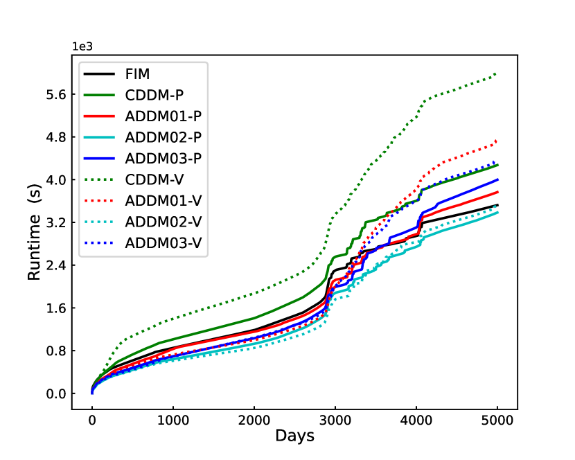
(a)

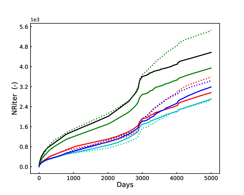
(b)

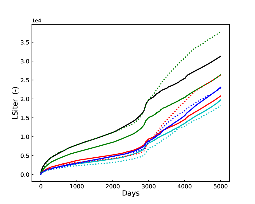
(c)

(d)

Figure 9: Figures (a), (b), (c), and (d) illustrate the performance of these methods from four perspectives: wall time from the first time step to the last time step (Runtime), cumulative global Newton-Raphson iterations (NRiter), cumulative global linear iterations (LSiter), and the ratio of LSiter to NRiter (LS/NR). The suffixes P and V denote constant pressure and constant component flux, respectively.

4.1.3 Different coupling strategies

Both CDDM and ADDM effectively reduce the global Newton-Raphson iterations and linear solver iterations (i.e., NRiter and LSiter). However, this reduction comes at the cost of solving numerous subproblems, which in turn introduces a significant number of Newton-Raphson and linear solver iterations for the subproblems. It can be anticipated that the more accurately the subproblems represent the global problem, the fewer NRiter and thereby LSiter will be required for the global problem to converge. However, more precise subproblems tend to be larger in size and incur higher solving costs. Therefore, to achieve better acceleration, finding the optimal tradeoff between the cost of solving the global problem and the subproblems is crucial. It can be seen from Figure 8 and Table 1 that the reduction in NRiter for CDDM, which completely ignores the important couplings between subdomains, is insufficient. Consequently, in terms of runtime, it offers no advantage over FIM and is even slower. Next, we focus on comparing different adaptive coupling strategies.

Figure 10 illustrates the changes in gas saturation relative to the previous time step at different time points, along with the corresponding subdomain coupling patterns for ADDM01, ADDM02, and ADDM03. Throughout the simulation, gas primarily accumulates in the upper layers; thus, we have presented the changes in gas saturation specifically for the topmost layer. In fact, the evolution pattern of the lower layer is the same as that of the upper layer, with only a time delay. It is important to note that the subdivision of domains is essentially two-dimensional; therefore, a single cross-section can effectively illustrate their coupling patterns. ADDM01 accurately captures domains with significant saturation changes and couples nearby intersecting subdomains for the solution. The number of subdomains involved in each coupling domain is relatively small, potentially enhancing the parallel efficiency of subproblem solving. Building on ADDM01, ADDM02 also accounts for the movement of these critical regions by using more subdomains to cover them. This further enhances the convergence performance of the global problem. However, this can result in large coupling domains, significantly increasing the cost of solving the subproblems, as shown in Figures 10(m). ADDM03 effectively controls the size of coupling domains and increases subdomain coupling to fully leverage parallel computing resources. However, it struggles to accurately capture critical regions when flow conditions become complex, as shown in Figure 10(t). This is the main reason for its sharp performance decline after the 3000th day.

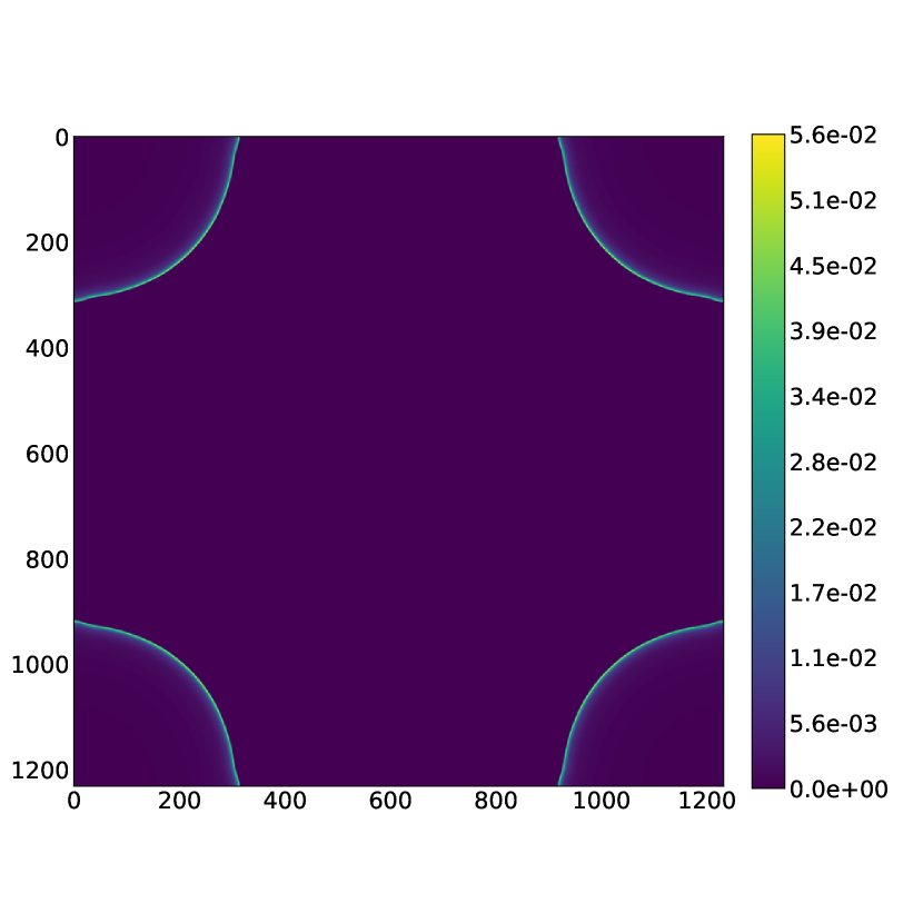
(a)

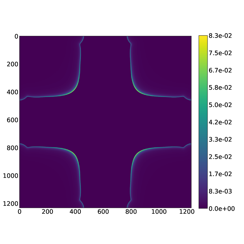
(b)

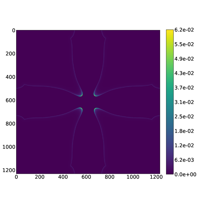
(c)

(d)

(e)

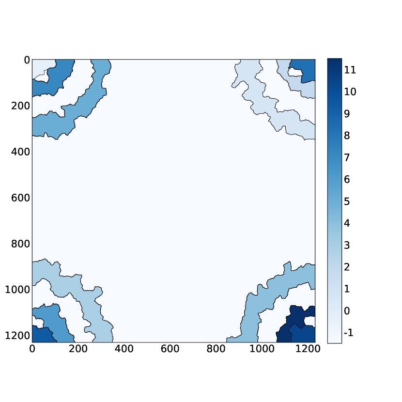
(f)

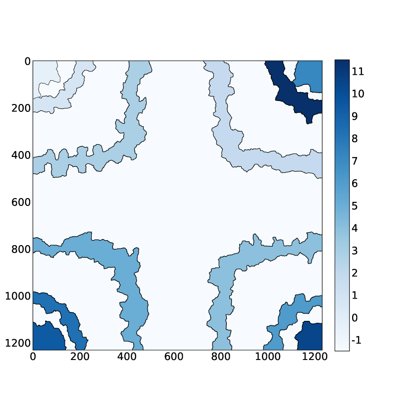
(g)

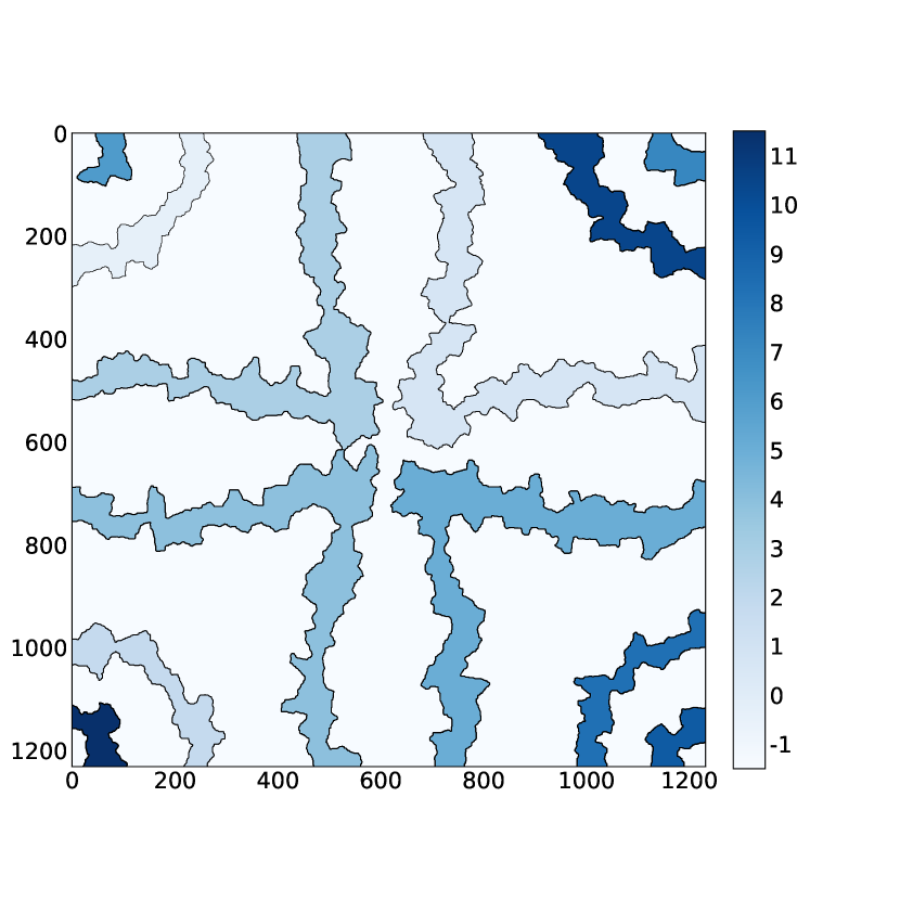
(h)

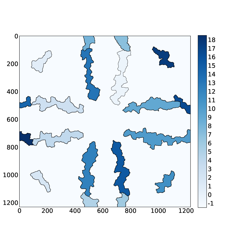
(i)

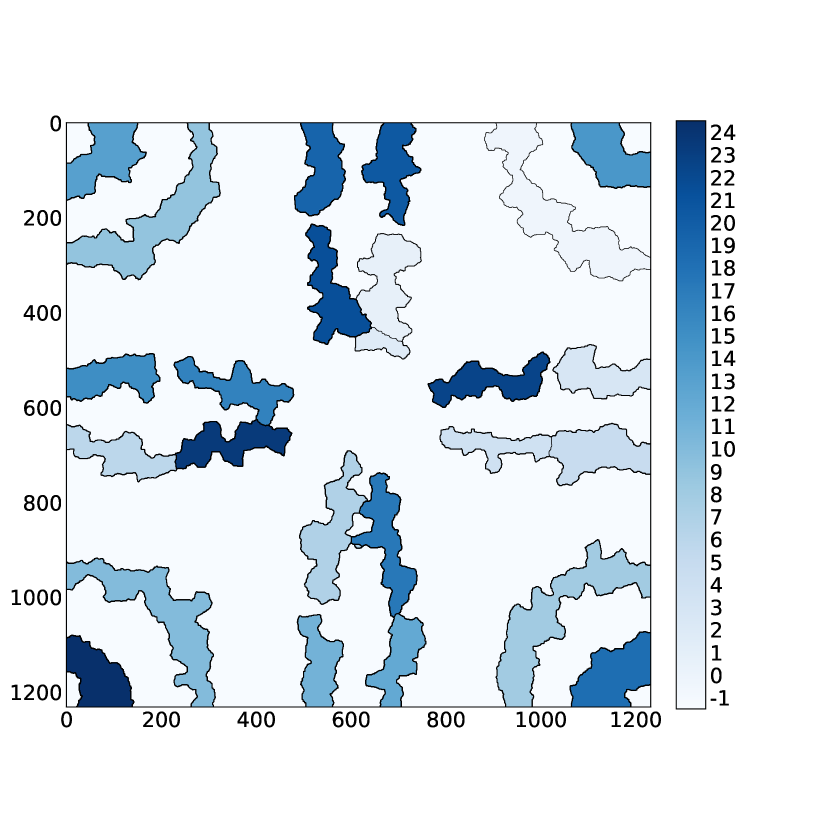
(j)

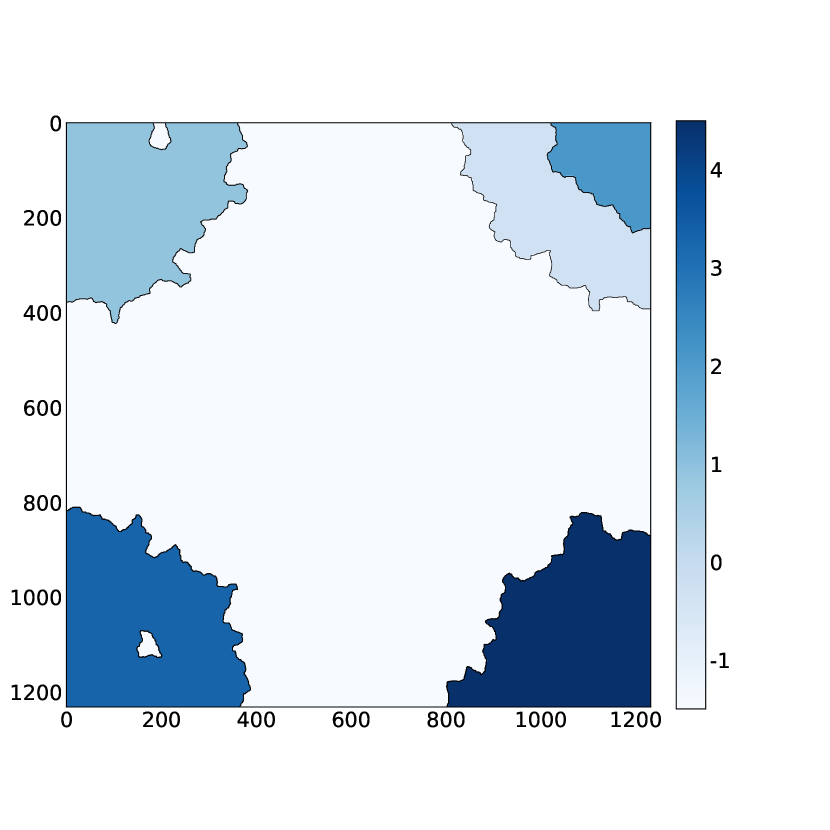
(k)

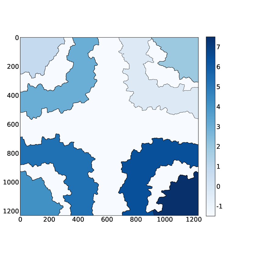
(l)

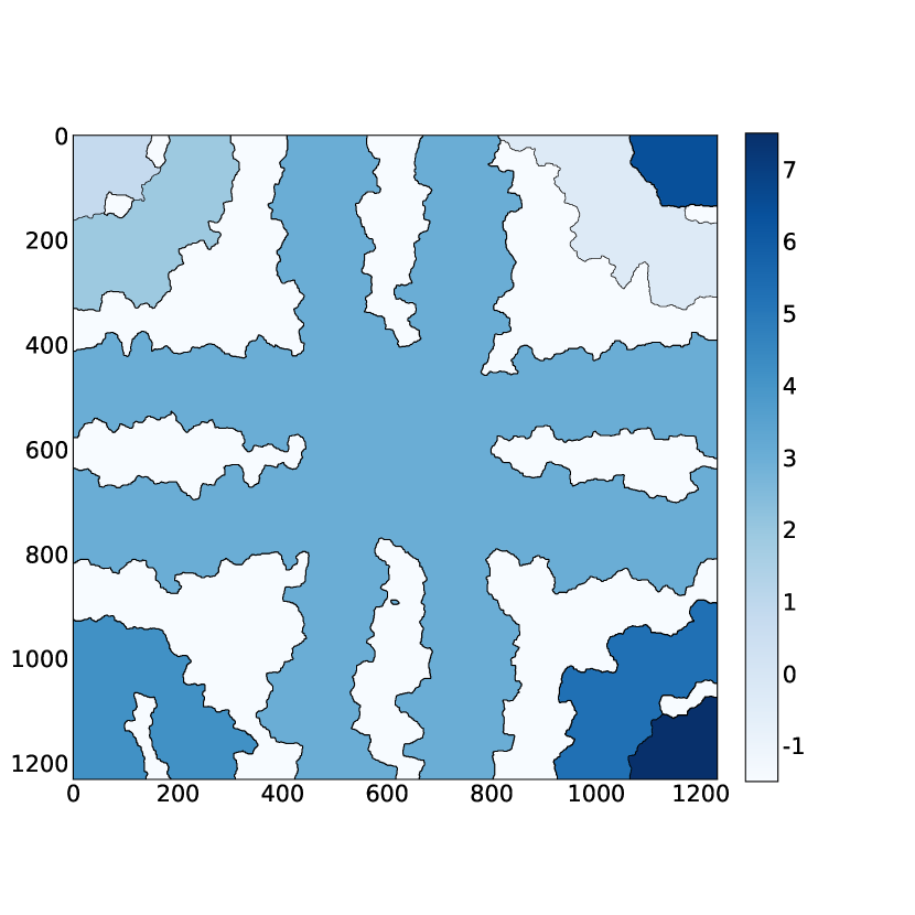
(m)

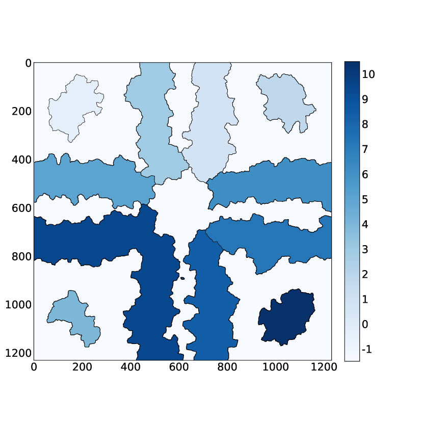
(n)

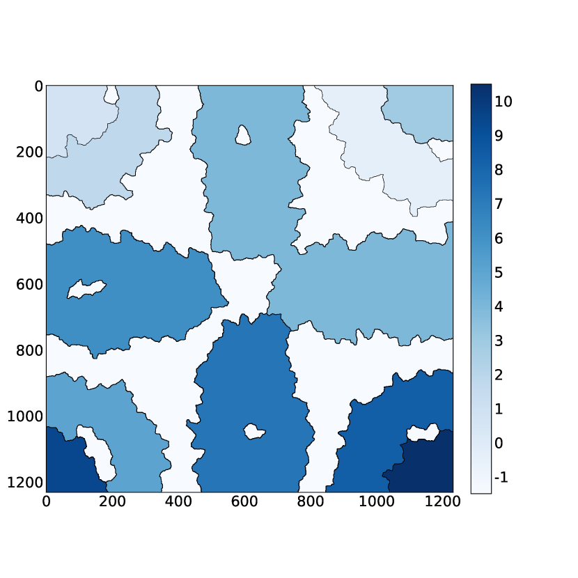
(o)

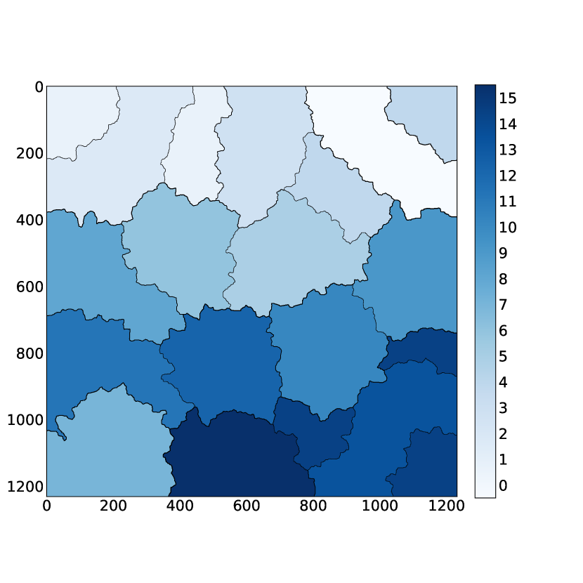
(p)

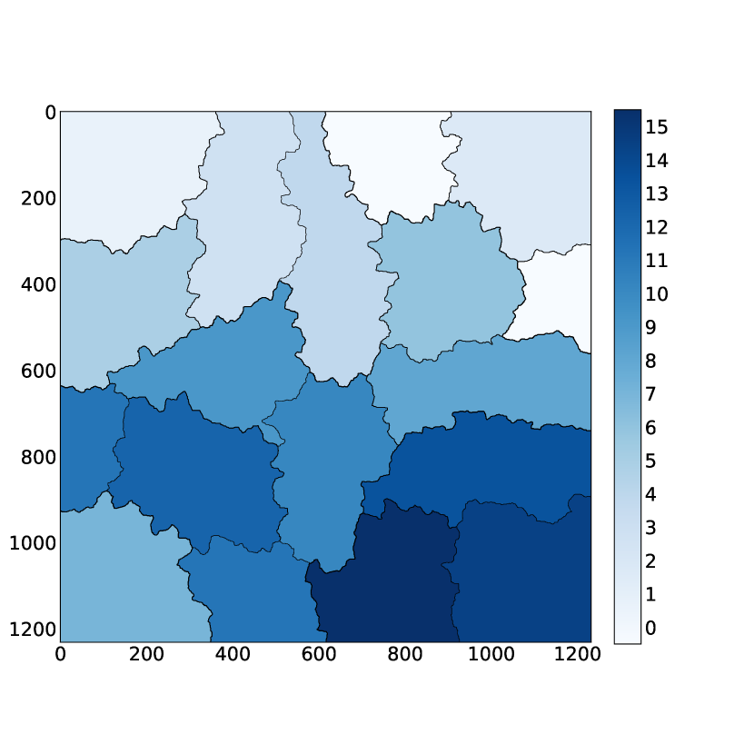
(q)

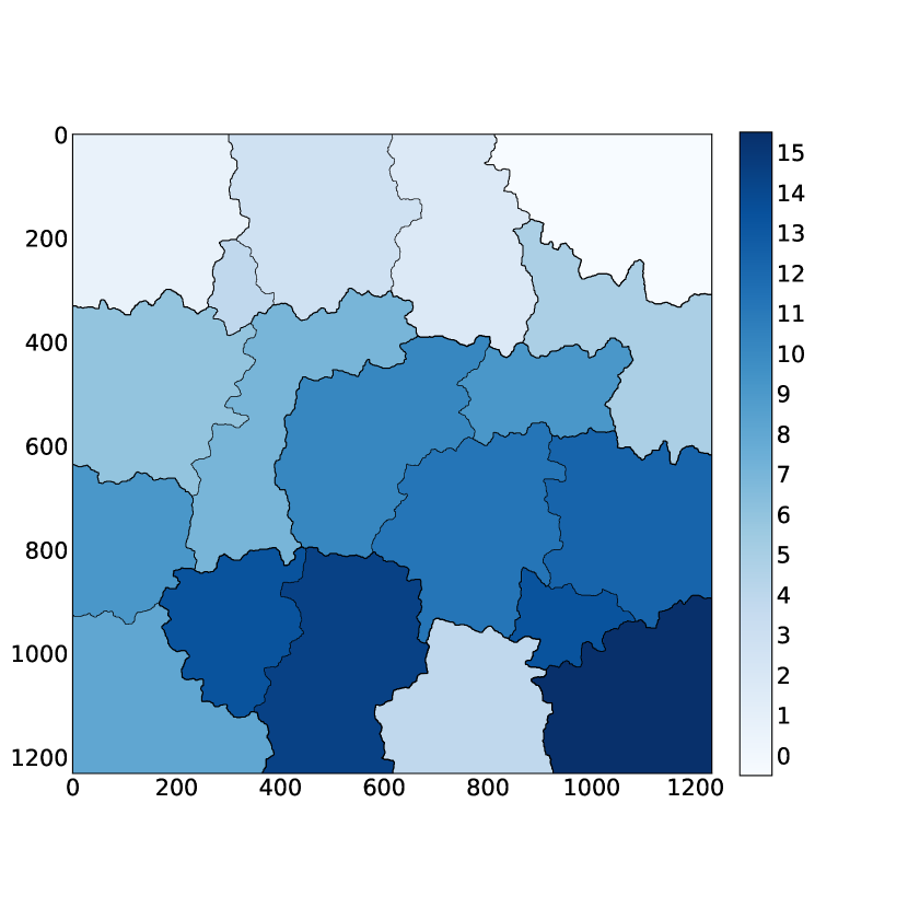
(r)

(s)

(t)

Figure 10: Figures (a) to (e) show the change in gas saturation relative to the previous time step in the top layer of the reservoir on days 750, 2000, 2820, 3000, and 5000, respectively. Figures (f) to (j), (k) to (o), and (p) to (t) respectively illustrate the subdomain coupling patterns for ADDM01, ADDM02, and ADDM03 at the corresponding time points. For ADDM01 and ADDM02, subdomains in the lightest areas (corresponding to a value of -1) are solved independently, while the remaining subdomains, marked with the same color (sharing common boundaries), are solved in a coupled manner. In ADDM03, there are no independently solved subdomains; all subdomains marked with the same color (sharing common boundaries) are solved in a coupled manner.

In all the previous results, we observed a consistent phenomenon: ADDM achieved significant performance improvements over FIM during the first 3000 days, with ADDM02 showing the most substantial acceleration, reaching a maximum speedup of 542 seconds (23.6%) on the 3000th day. However, after 3000 days, performance sharply declined, eventually losing its acceleration advantage. We speculate that this decline is related to the increasing complexity of the flow conditions, which caused the adopted adaptive coupling strategy to fail in accurately capturing the flow characteristics. Before gas breakthrough to the production well (approximately the first 3000 days), the direction of gas movement was consistent with the direction of pressure propagation, making it sufficient to capture the domains with the greatest gas saturation changes. However, after the gas breakthrough, the reservoir pressure declined rapidly overall, which did not align with the direction of gas movement. Consequently, this strategy became ineffective, and from the 3000th day onward, all ADDM approaches were slower than FIM.

Next, we will compare the selection of parameter $c_{{}_{S}}$ in different subdomain coupling strategies for ADDM in more detail. Given the poor adaptability of ADDM03, our comparison will be limited to ADDM01 and ADDM02. We considered four different selections for $c_{{}_{S}}$: ADDM-A, ADDM-B, ADDM-C, and ADDM-D, all of which have been previously discussed. Figure 11 shows the subdomain coupling patterns of ADDM01-B and ADDM02-B at several key time points. Since the results for ADDM-C and ADDM-D are similar to those for ADDM-B, they are not displayed. Compared to the ADDM-A version shown in Figure 10, ADDM-B, ADDM-C, and ADDM-D exhibit larger coupling areas, resulting in overall acceleration for ADDM01, as listed in Table 2. This indicates that there remains substantial room for optimization in the parameter ($c_{{}_{S}}$) selection of its coupling strategy.

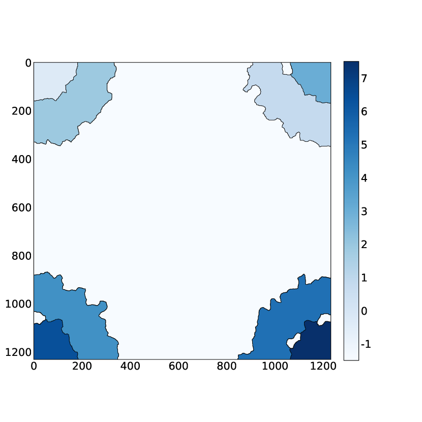
(a)

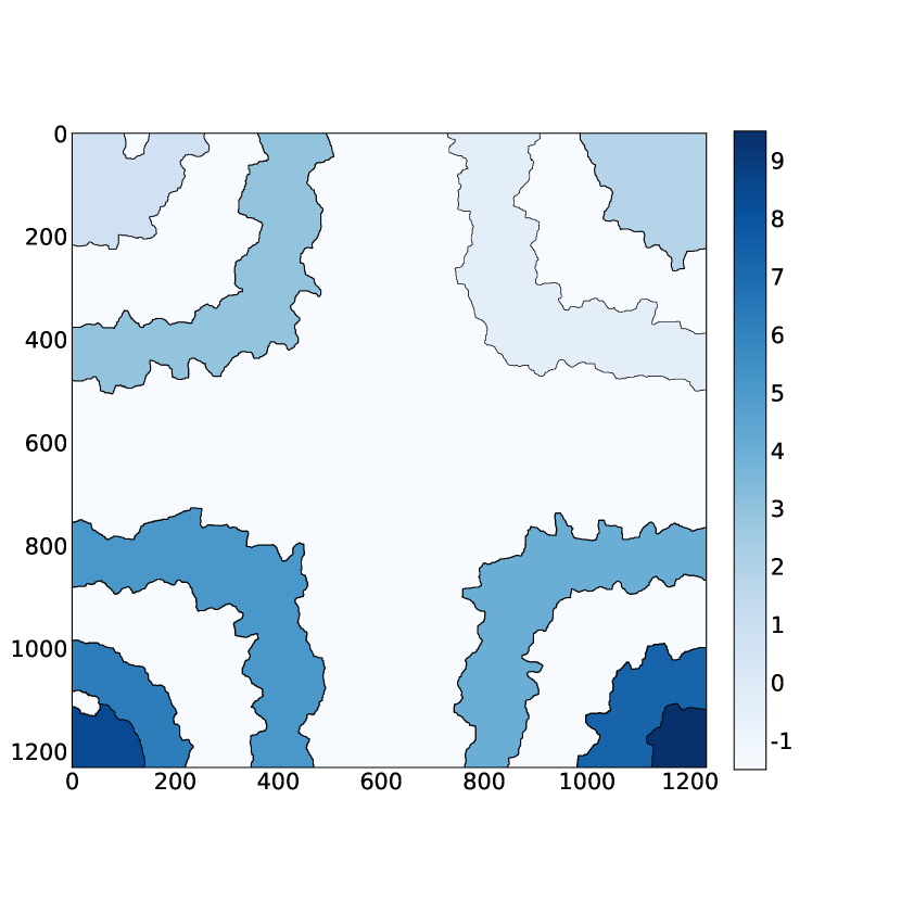
(b)

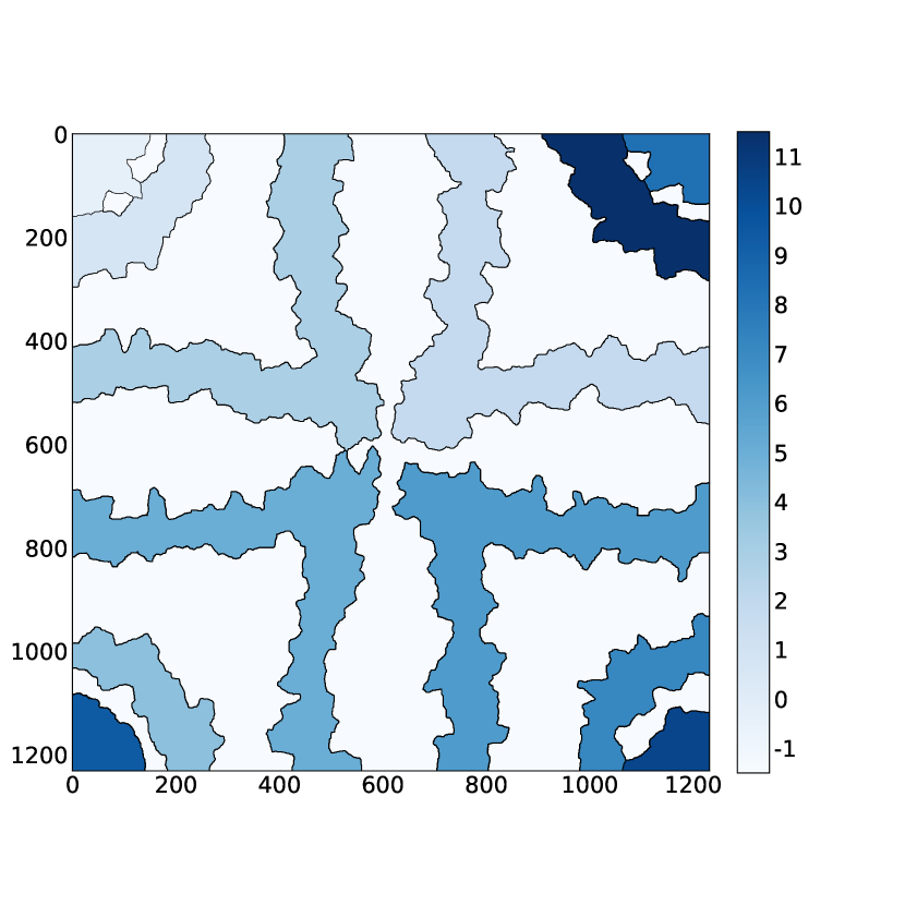
(c)

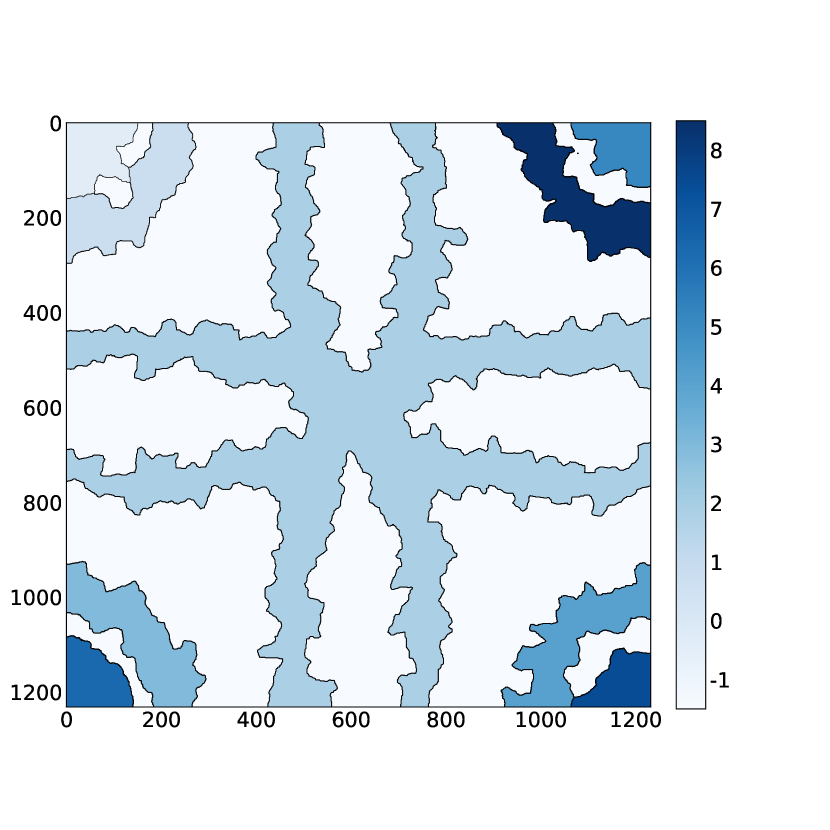
(d)

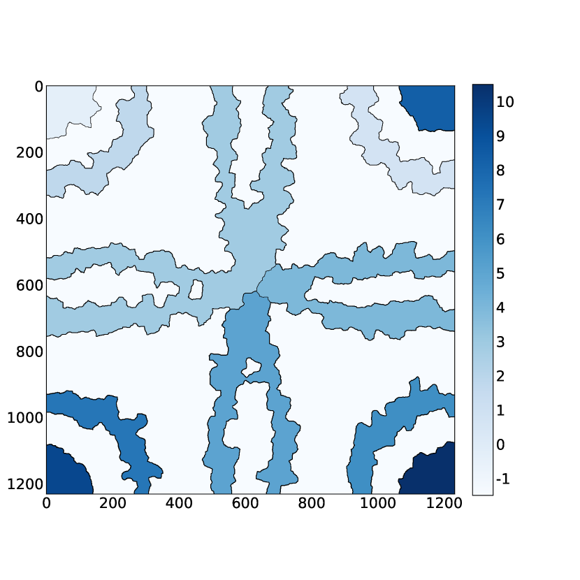
(e)

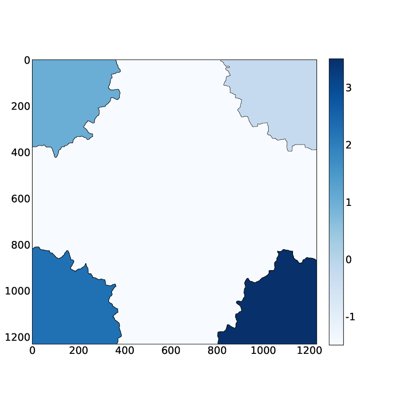
(f)

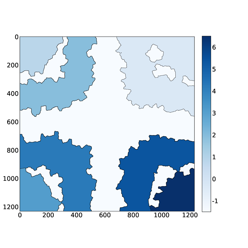
(g)

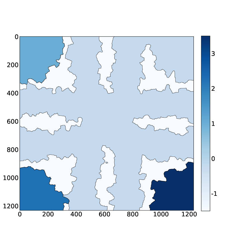
(h)

(i)

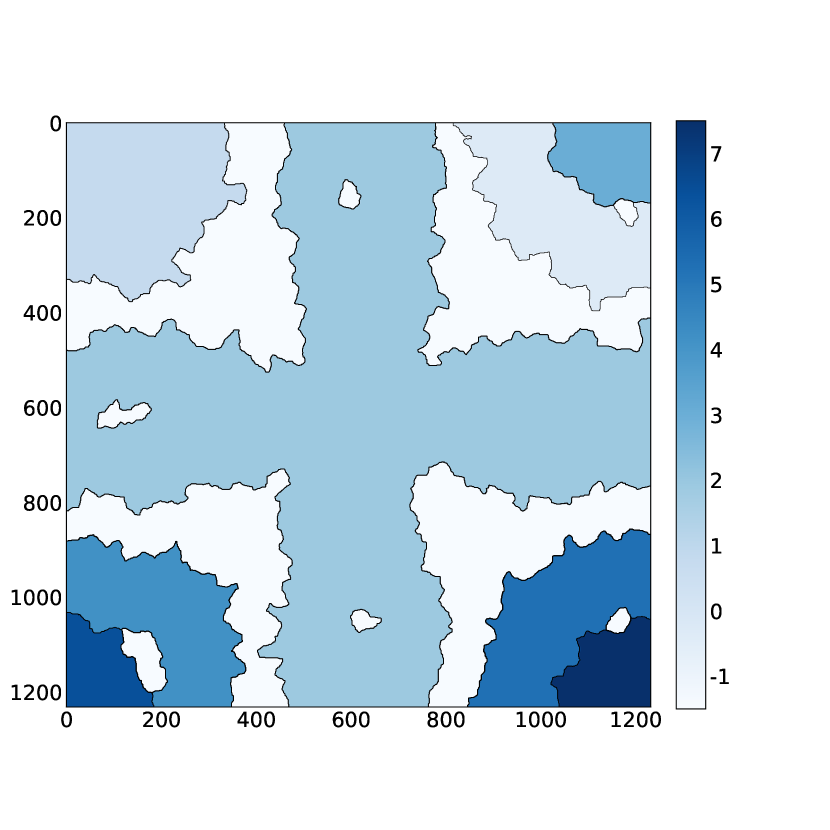
(j)

Figure 11: Figures (a) to (e), and (f) to (j) respectively illustrate the subdomain coupling patterns for ADDM01-B and ADDM02-B on days 750, 2000, 2820, 3000, and 5000, respectively.

Table 2: Cumulative wall time (s) of each method at key time points, starting from the first time step. Bold indicates the best performance results.

Method	60d	750d	2000d	2600d	2820d	3000d	4000d	5000d
FIM	254	756	1185	1512	1716	2301	2946	3523
ADDM01-A	183	639	995	1262	1430	2002	3817	4740
ADDM01-B	169	564	915	1179	1340	1848	2917	3644
ADDM01-C	181	586	930	1200	1365	1865	2744	3437
ADDM01-D	183	596	941	1211	1384	1888	3120	3972
ADDM02-A	163	537	849	1106	1263	1759	2831	3513
ADDM02-B	179	570	888	1151	1313	1733	2641	3026
ADDM02-C	174	549	875	1136	1296	1845	2621	3077
ADDM02-D	179	567	892	1156	1320	1803	2719	3142

For ADDM02, before gas breakthrough to the production well (approximately before the 3000th day), the larger coupling area slowed down the simulation process. However, after the gas breakthrough, its advantages became evident, especially from the 4000th to the 5000th day, where it demonstrated acceleration compared to FIM. For instance, ADDM02-B accelerated by 192 seconds (33.3%) compared to FIM in the time interval from the 4000th to the 5000th day.

Figure 12 compares the performance of these strategies using several key indicators. It can be observed that, compared to ADDM-A, ADDM-B, ADDM-C, and ADDM-D each significantly reduced LSiter and lowered the LS/NR ratio. Particularly for ADDM02, this resulted in a slower increase in these two metrics compared to FIM in the later stages of the simulation, thereby continually gaining an acceleration advantage. Furthermore, improved coupling strategies enhance the robustness of the simulation. They reduce wasted cumulative global Newton-Raphson iterations while maintaining the same Newton-Raphson iterations for subproblems, thereby further accelerating the simulation process, as illustrated in Figures 12(c) and 12(d).

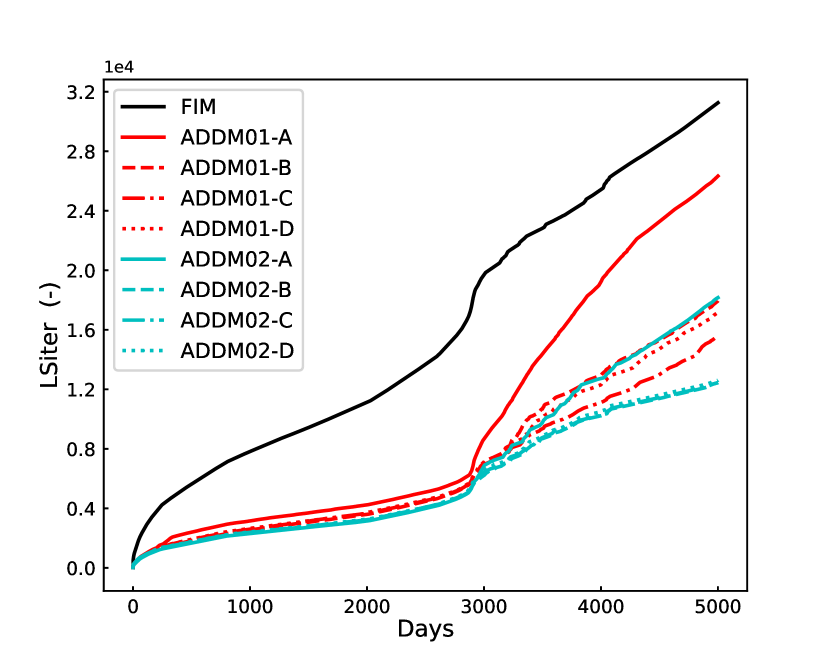
(a)

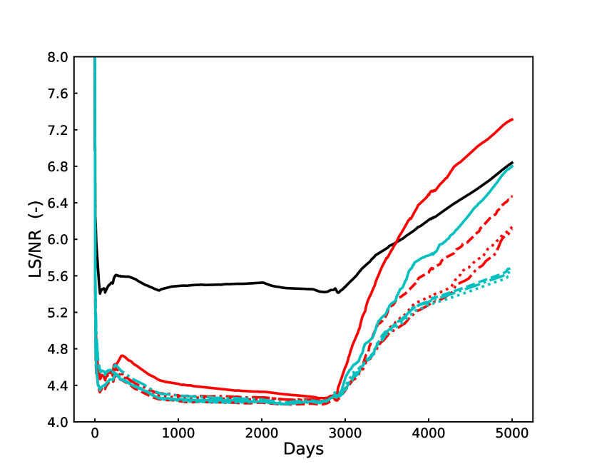
(b)

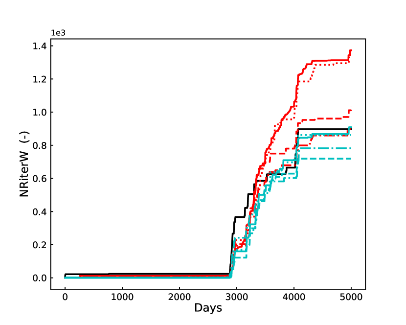
(c)

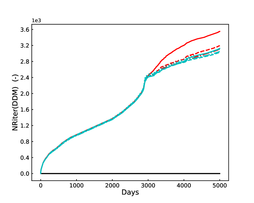
(d)

Figure 12: Figures (a), (b), (c), and (d) illustrate the performance of these methods from four perspectives: wall time from the first time step to cumulative global linear iterations (LSiter), the ratio of LSiter to NRiter (LS/NR), wasted cumulative global Newton-Raphson iterations (NRiterW), and cumulative Newton-Raphson iterations for subproblems in DDM.

4.2 Case 2

Case 2 examines the performance of the ADDM method in heterogeneous media. The original SPE1 case features a three-layer geological structure with horizontal rock permeability values of 500mD, 50mD, and 200mD, respectively. In Case 1, due to vertical grid refinement, these layers correspond to grid layers 1 to 2, 3 to 5, and 6 to 10, respectively. Building on Case 1, we modified the horizontal permeability of these three geological layers to introduce heterogeneity. As shown in Figure 13, the horizontal permeability in each layer follows a Gaussian distribution, with the mean values remaining consistent with the original case.

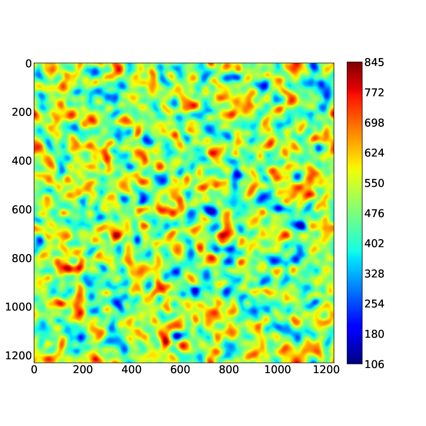
(a)

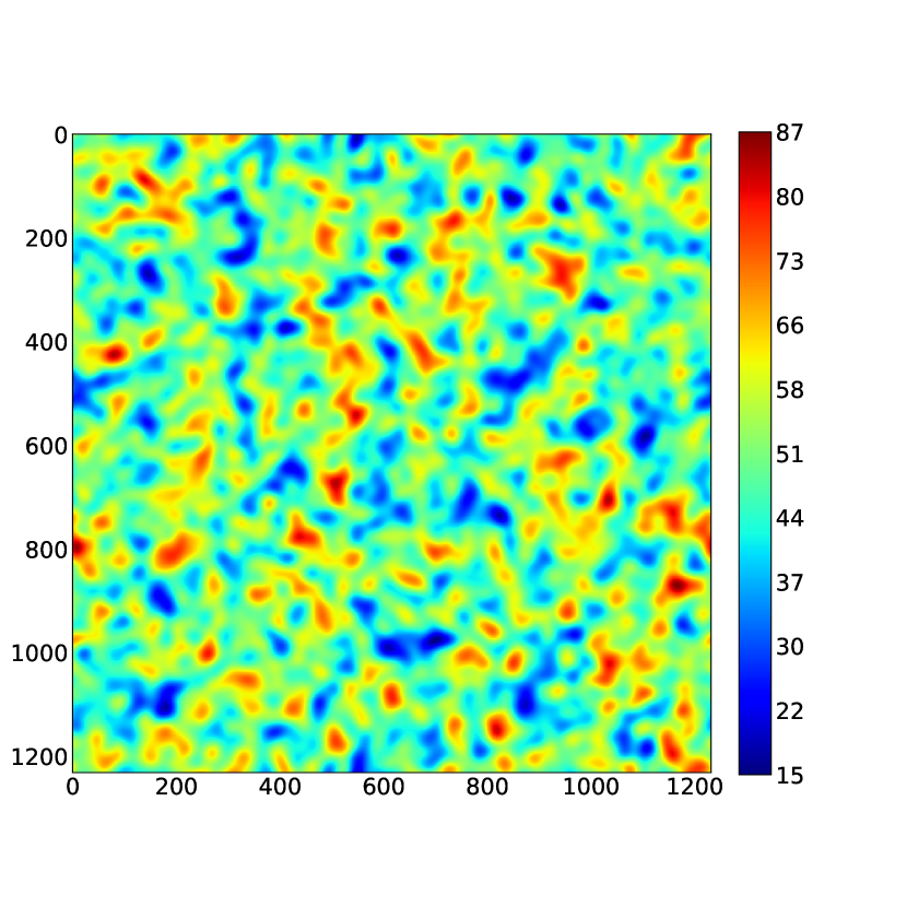
(b)

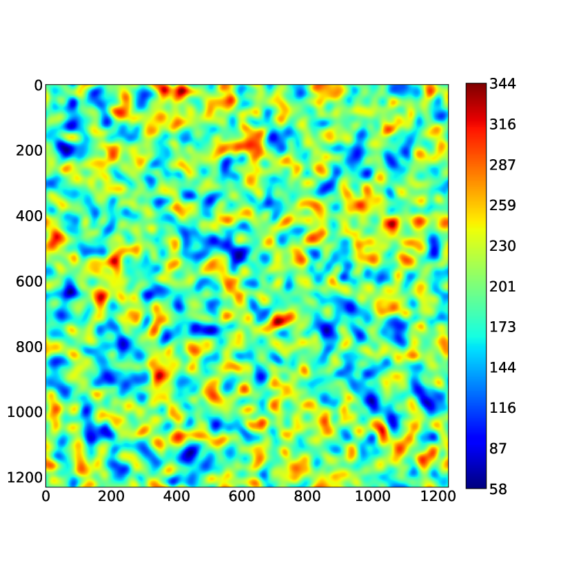
(c)

Figure 13: Figures (a), (b), and (c) represent the horizontal permeability for grid layers 1 to 2, 3 to 5, and 6 to 10, respectively.

In this study, we compared FIM, ADDM01, and ADDM02, utilizing parameter ($c_{{}_{S}}$) selection strategy B. We simulated a total period of 3000 days using 784 processes. Figures 14(a) to 14(e) present the gas saturation distribution in the topmost layer at various critical time points, demonstrating a noticeably more complex flow pattern compared to Case 1. Figures 14(f) to 14(j) and Figures 14(k) to 14(o) illustrate the subdomain coupling patterns of ADDM01 and ADDM02 at corresponding time points, respectively. It can be observed that the subdomains exhibit more complex coupling patterns. For ADDM01, the coupling domains are more fragmented and irregular. In contrast, ADDM02, with its broader coupling area, encompasses most of the subdomains, leaving the excluded subdomains dispersed within the coupling domain.

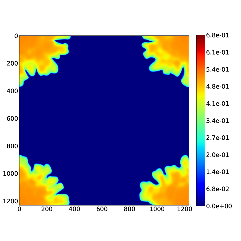
(a)

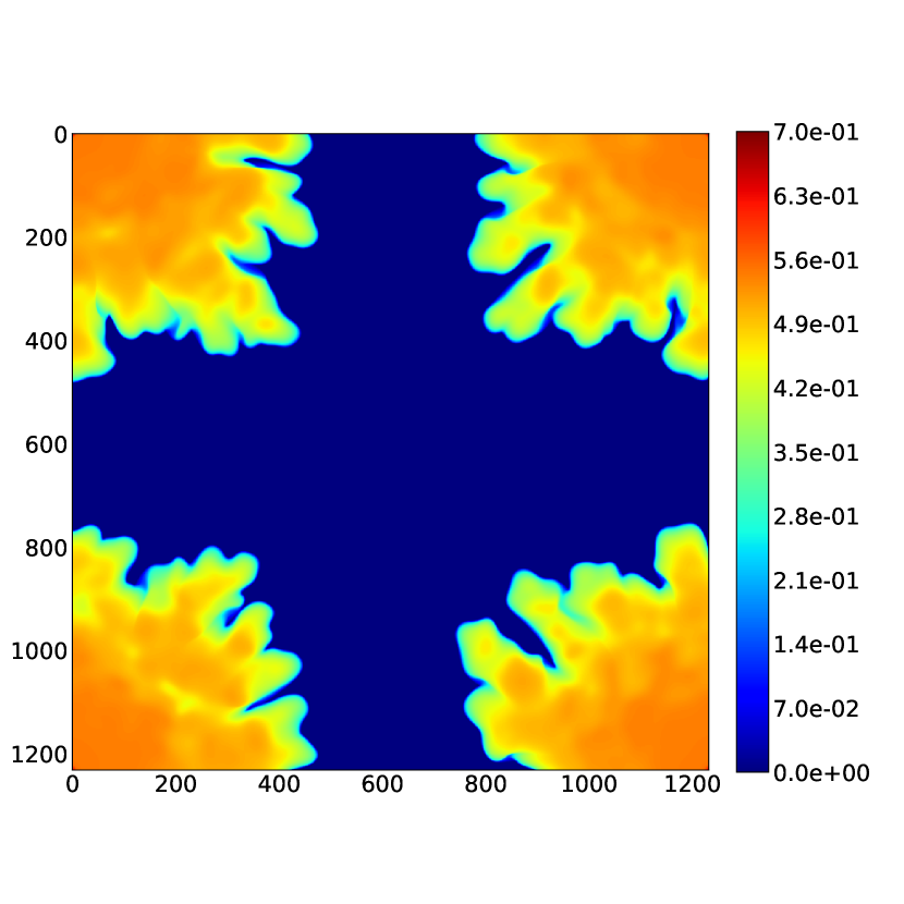
(b)

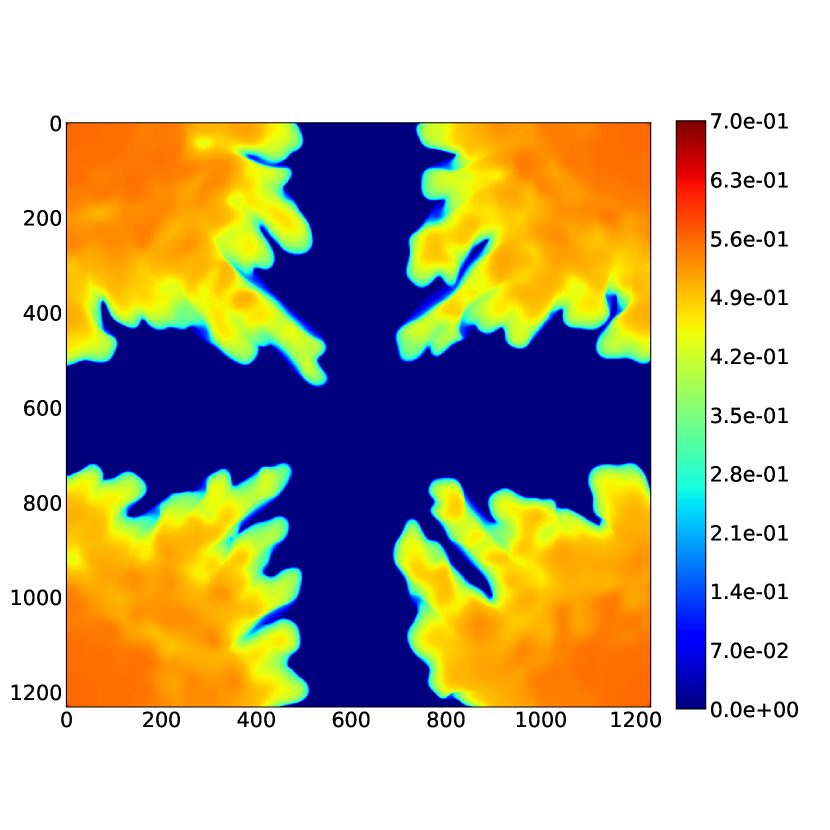
(c)

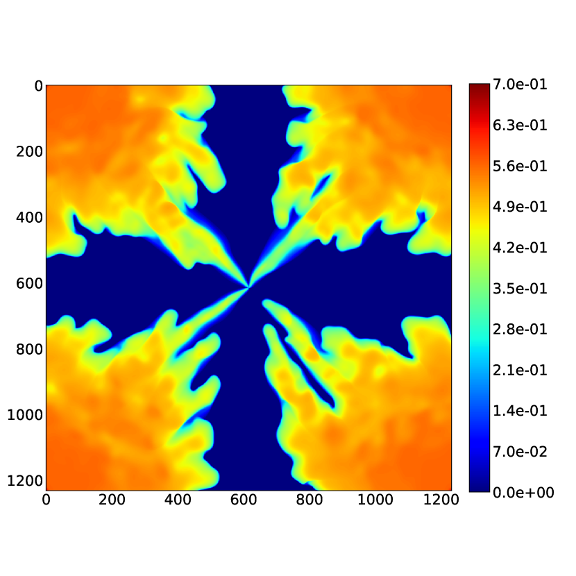
(d)

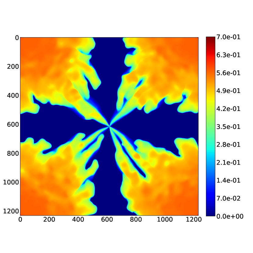
(e)

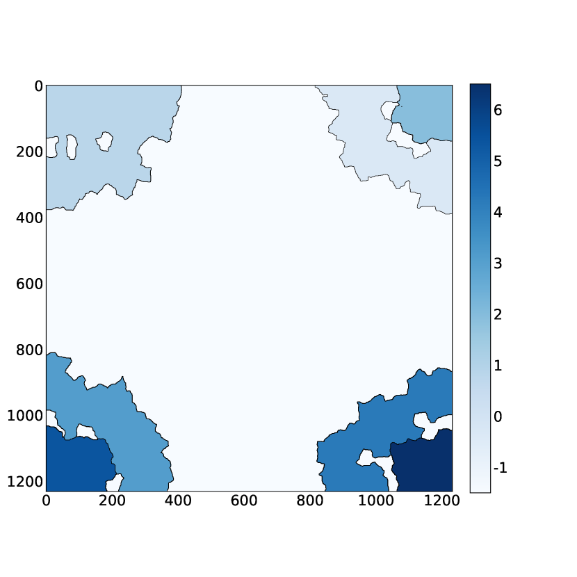
(f)

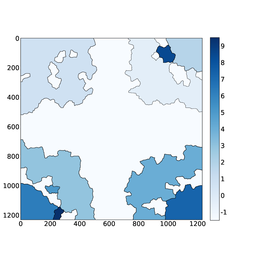
(g)

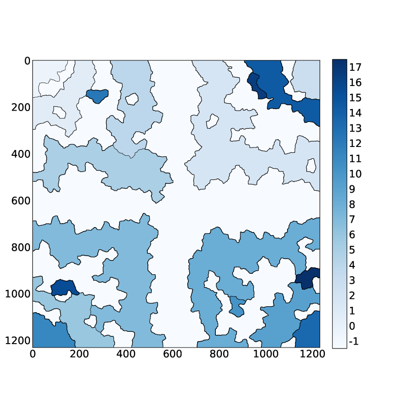
(h)

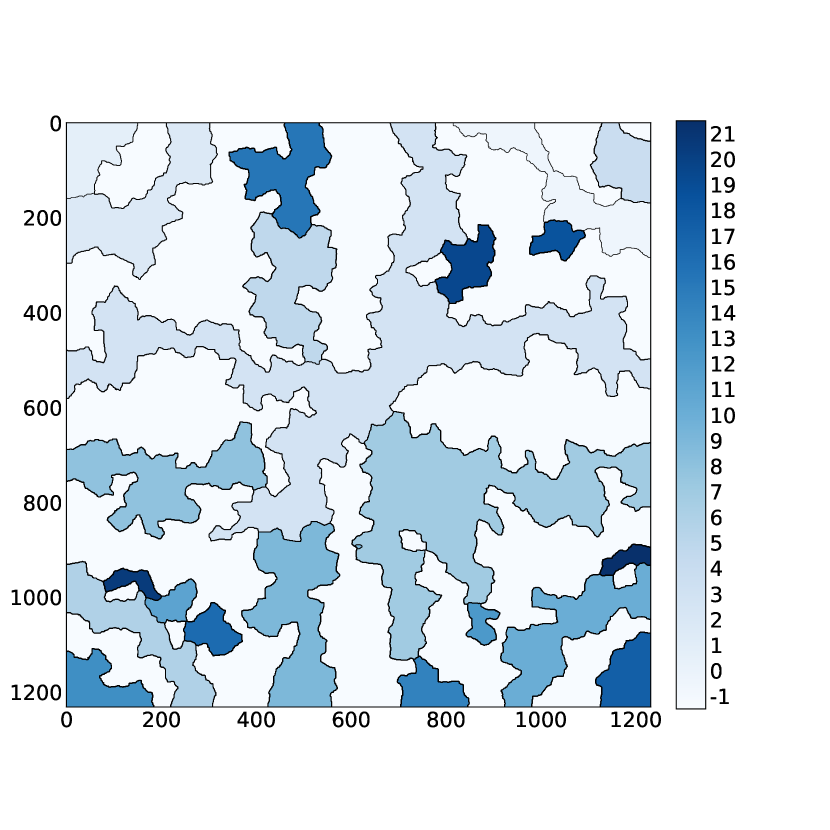
(i)

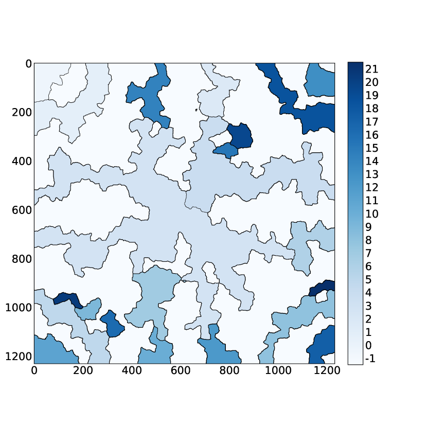
(j)

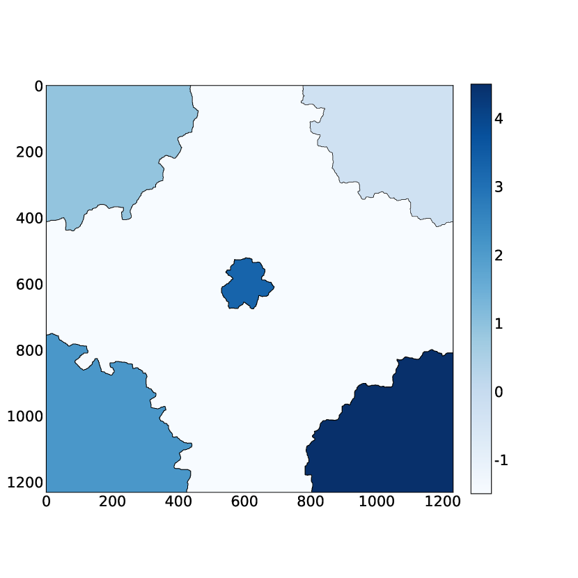
(k)

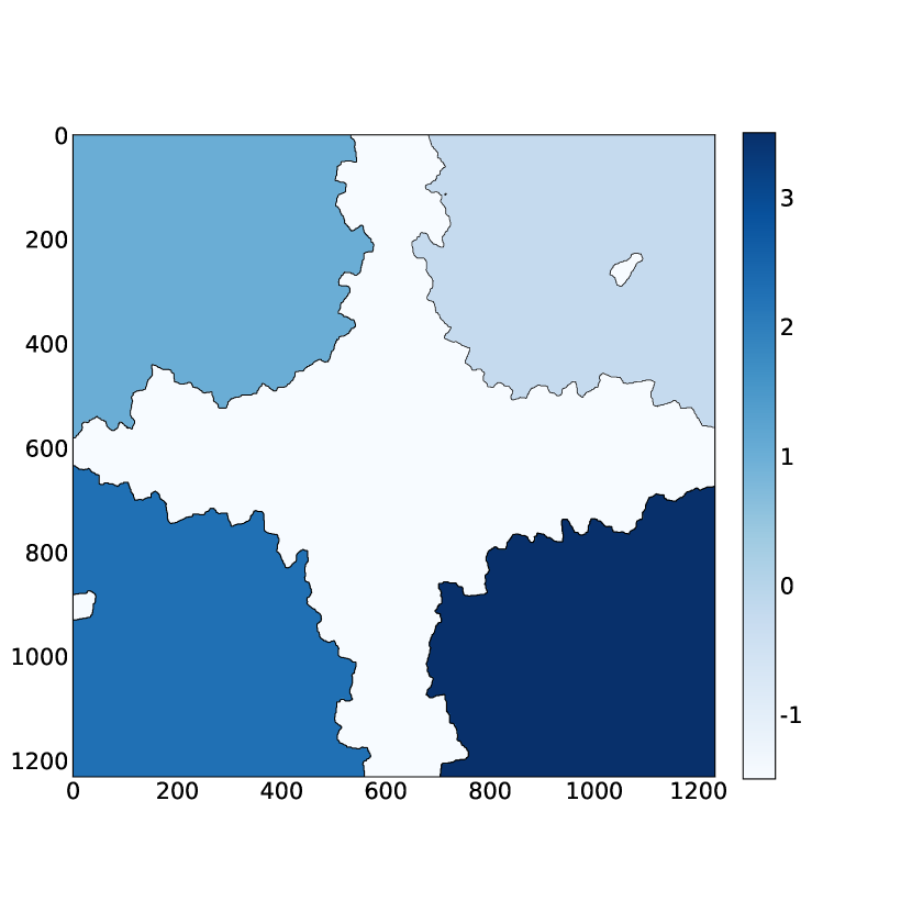
(l)

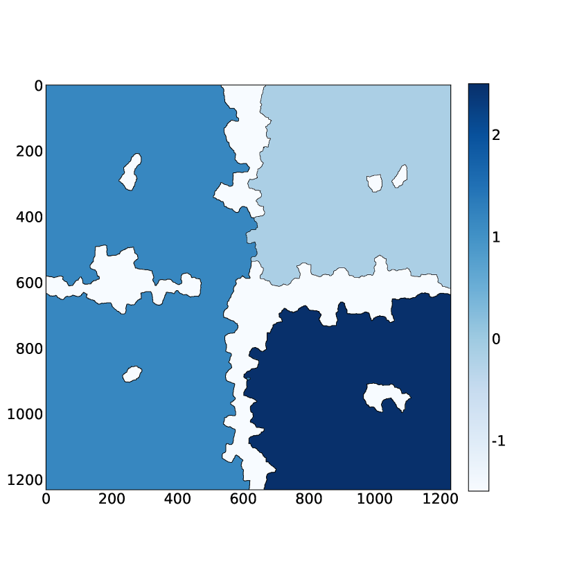
(m)

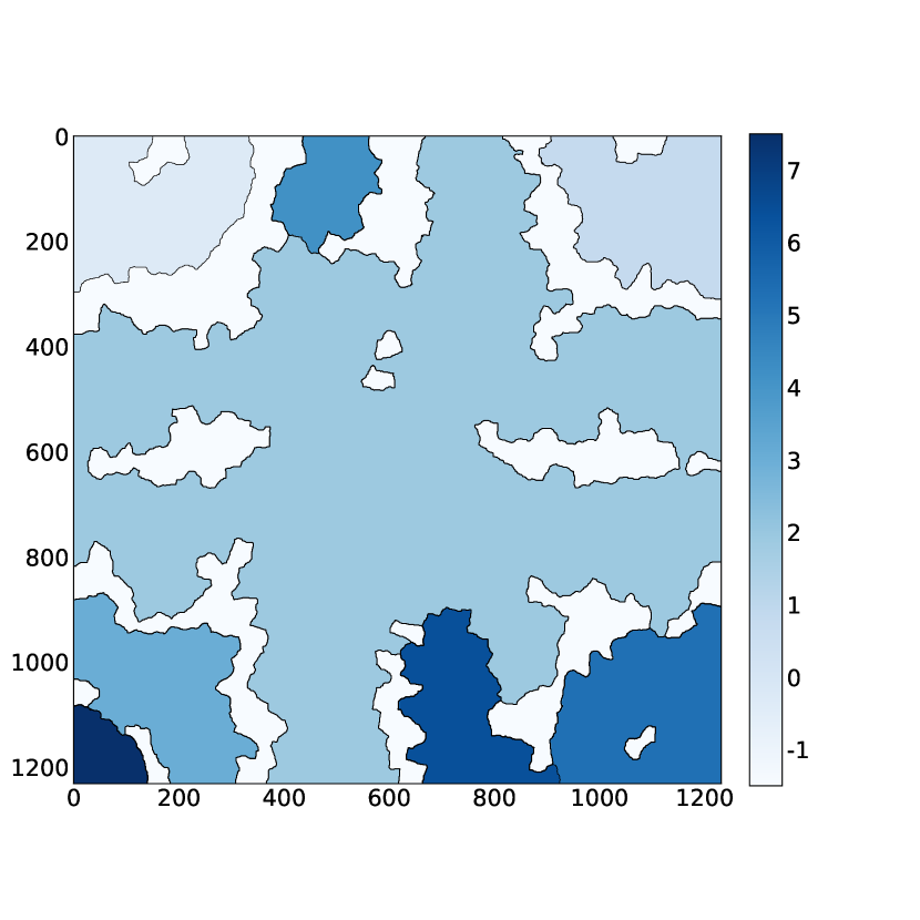
(n)

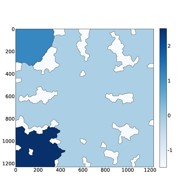
(o)

Figure 14: Figures (a) to (e) illustrate the gas saturation distribution in the topmost layer on days 900, 1800, 2400, 2800, and 3000. Figures (f) to (j) and Figures (k) to (o) illustrate the subdomain coupling patterns of ADDM01 and ADDM02 at these time points, respectively.

Figures 15(a) compares the field gas production rates obtained from the three methods, verifying the consistency of their results. As shown in Figures 15(b) and 15(c), ADDM01 and ADDM02 significantly reduce the NRiter and LSiter, and exhibit a slower growth rate. Additionally, they consistently maintain a lower ratio of LSiter to NRiter, as presented in Figure 15(d). Furthermore, these two methods exhibit a significant advantage in controlling wasted global Newton-Raphson iterations, which is a crucial factor in further enhancing their computational performance, as illustrated in Figure 15(e). Notably, compared to Case 1 (the simpler scenario), ADDM achieved a more significant reduction in NRiter and LSiter in Case 2, demonstrating that ADDM maintains robust performance even for more complex problems. Figure 15(h) shows the computation times for the three methods. On day 3000, ADDM01 achieved a speedup of 674 seconds (18.7%) compared to FIM, while ADDM02 achieved a speedup of 569 seconds (15.8%). Additionally, Figure 15(h) reveals that ADDM02 maintains an advantage over ADDM01 for at least the first 2750 days, as it reduces more NRiter and LSiter at a reasonable cost. However, after this period, ADDM02 begins to lag behind ADDM01 because it couples too many subdomains, resulting in costs that outweigh the benefits, as shown in Figures 14(n) and 14(o). On the other hand, as ADDM02 couples more subdomains, its behavior becomes increasingly similar to that of FIM. As shown in Figure 15(g), ADDM02 has more NRiterW(DDM) compared to ADDM01, and the trend of this curve aligns closely with that of FIM in Figure 15(e). The rapidly increasing NRiterW(DDM) is also a key factor contributing to ADDM02’s slower performance relative to ADDM01 in the later stages of the simulation. Nevertheless, ADDM02 still demonstrates advantages over FIM.

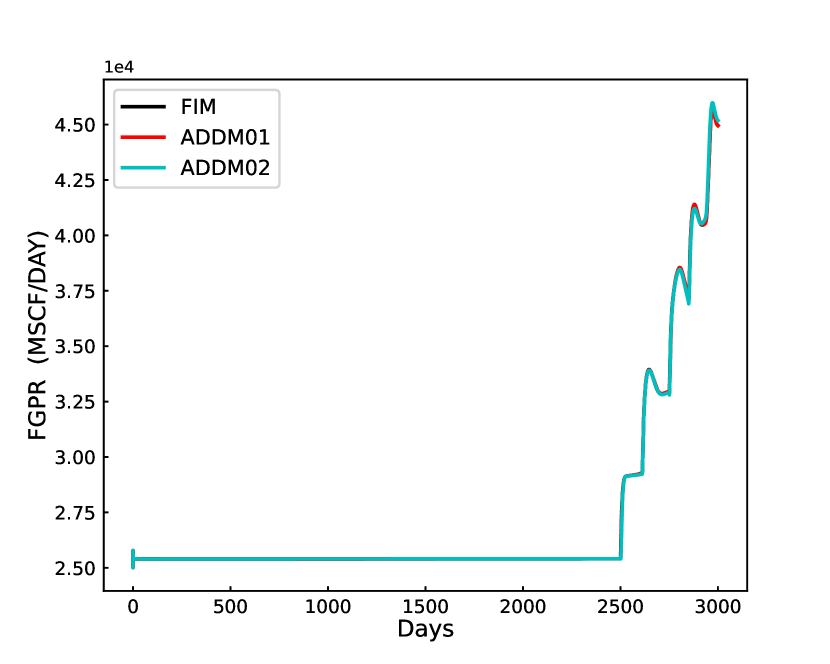
(a)

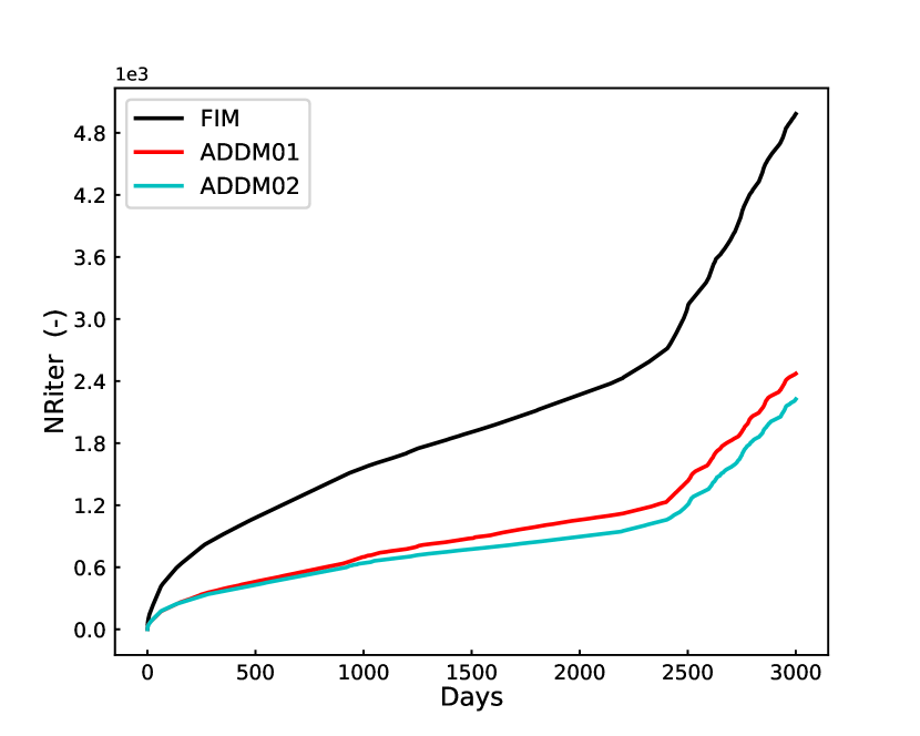
(b)

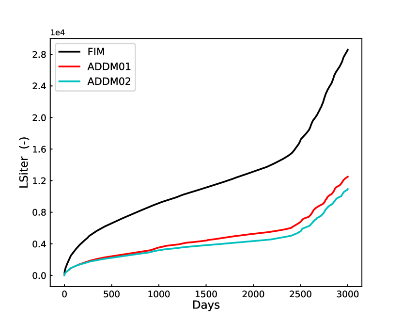
(c)

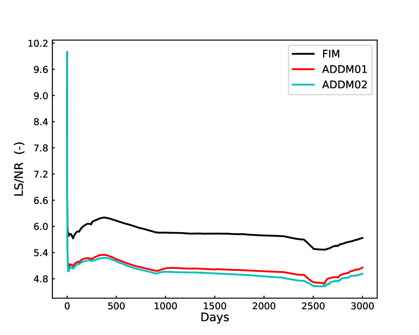
(d)

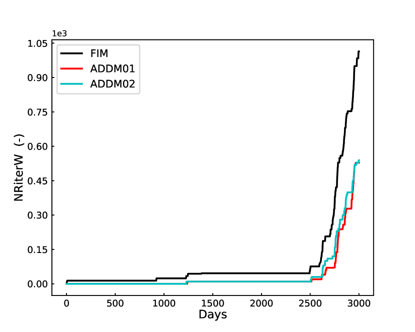
(e)

(f)

(g)

(h)

Figure 15: Figures (a) field gas production rate, respectively. Figures (b) to (h) illustrate the computational performance of the three methods from following perspectives: the cumulative global Newton-Raphson iterations (NRiter), the cumulative global linear iterations (LSiter), the ratio of LSiter to NRiter (LS/NR), wasted cumulative global Newton-Raphson iterations (NRiterW), cumulative Newton-Raphson iterations for subproblems in DDM (NRiter(DDM)), wasted cumulative Newton-Raphson iterations for subproblems in DDM (NRiterW(DDM)), and wall time (Runtime).

4.3 Parallel scalability

The last subsection focuses on the weak scaling study of the proposed method, with numerical simulations involving over 2 billion degrees of freedom and more than 10000 processes. The weak scalability is used to evaluate parallel performance while keeping the problem size per processor constant. For the scalability tests, we conduct numerical simulations on the aforementioned three-dimensional Case 1, simulating a total period of 1000 days. The simulation starts with a $791\times 791\times 25$ mesh size using 384 processes and ends with a $3164\times 3164\times 50$ mesh size, which includes 2,002,179,200 degrees of freedom, computed on 12288 processes, with each process handling 160,000 degrees of freedom. We tested the FIM, CDDM, and ADDM02 methods in this study, with strategy A applied to $c_{{}_{S}}$ in ADDM02. Table 3 lists the different mesh sizes, number of processes (Np), number of time steps (Timestep), cumulative global Newton-Raphson iterations (NRiter), and cumulative global linear iterations (LSiter). Figure 16 presents the cumulative linear solver time (LStime) and total simulation time (Totaltime).

Table 3: The weak scaling results by using different numbers of processes for the FIM, CDDM, and ADDM02 methods. Bold indicates the best performance results.

Mesh	Np	Method	Timestep	NRiter	LSiter
$791\times 791\times 25$	384	FIM	181	577	4520
		CDDM	181	436	3940
		ADDM02	181	301	2755
$1582\times 1582\times 25$	1536	FIM	185	679	5881
		CDDM	185	742	5957
		ADDM02	185	341	3099
$1582\times 1582\times 50$	3072	FIM	181	851	7739
		CDDM	192	932	8628
		ADDM02	181	360	4381
$3164\times 3164\times 50$	12288	FIM	189	1002	10531
		CDDM	261	1435	14849
		ADDM02	191	425	4912

It is well known that as grid refinement increases, the nonlinearity of the problem intensifies, and the condition number of the matrix for the system of linear equations worsens. This poses challenges for both the nonlinear and linear solvers. As shown in Table 3, compared to the FIM, CDDM can reduce the number of NRiter and LSiter to some extent for the smallest problem size, but this reduction is not sufficient to achieve a time efficiency advantage. Moreover, as the grid is refined, both NRiter and LSiter increase rapidly, even surpassing FIM. Particularly at the maximum mesh size of $3164\times 3164\times 50$, CDDM experiences frequent non-convergence issues, requiring repeated time step reductions and recalculations. In contrast, ADDM02 exhibits notable advantages. As the mesh is refined, the reductions in NRiter and LSiter compared to FIM increase from 47.8% and 39.1% to 57.6% and 53.4%, respectively. This indicates that the ADDM02 method is highly competitive in terms of convergence. Furthermore, as shown in Figure 16, CDDM requires longer LStime and Totaltime, while ADDM02 uses significantly less LStime and Totaltime. Notably, as the number of processes increases, the LStime and Totaltime for all three methods also increase, but ADDM02 exhibits the slowest growth rate. These results suggest that the ADDM method achieves good parallel performance and outperforms both CDDM and FIM in terms of weak scalability.

(a)

(b)

Figure 16: Figures (a) and (b) represent the cumulative linear solver time (LStime) and total simulation time (Totaltime) by using different numbers of processors for the FIM, CDDM, and ADDM02 methods, respectively.

5.   Conclusions

In this work, we proposed an adaptively coupled domain decomposition methods (ADDM) framework for the fully implicit solution of multiphase and multicomponent flow in porous media. The solution methods developed within this framework effectively capture strong nonlinearities in global problems by defining subproblems in the coupled regions based on fluid flow characteristics, significantly accelerating the convergence of nonlinear solvers. Furthermore, we introduced several adaptive coupling strategies and developed a nonlinear problem initialization method within this framework. Numerical experiments have confirmed the effectiveness of the proposed ADDM framework, which has demonstrated good parallel performance on a supercomputer with tens of thousands of processors for problems involving 2 billion degrees of freedom. In the future, we will explore applying the ADDM method to preconditioning techniques.

Conflicts of Interest

The authors declare that they have no known competing financial interests or personal relationships that could have appeared to influence the work reported in this paper.

References

- [1] K. Aziz, Petroleum reservoir simulation, vol. 476. Applied Science Publishers, 1979.
- [2] Z. Chen, G. Huan, and Y. Ma, Computational methods for multiphase flows in porous media. SIAM, 2006.
- [3] M. Zhang, H. Yang, S. Wu, and S. Sun, “Parallel multilevel domain decomposition preconditioners for monolithic solution of non-isothermal flow in reservoir simulation,” Computers & Fluids, vol. 232, p. 105183, 2022.
- [4] L. Zhao, C. Feng, C.-S. Zhang, and S. Shu, “Parallel multi-stage preconditioners with adaptive setup for the black oil model,” Computers & Geosciences, vol. 168, p. 105230, 2022.
- [5] L. Zhao, S. Li, C.-S. Zhang, C. Feng, and S. Shu, “An improved multistage preconditioner on GPUs for compositional reservoir simulation,” CCF Transactions on High Performance Computing, vol. 5, pp. 144–159, 2023.
- [6] J. Douglas, Jim, D. Peaceman, and J. Rachford, H.H., “A method for calculating multi-dimensional immiscible displacement,” Transactions of the AIME, vol. 216, pp. 297–308, 12 1959.
- [7] K. H. Coats, “IMPES Stability: The CFL Limit,” SPE Journal, vol. 8, pp. 291–297, 09 2003.
- [8] H. Yang, S. Sun, Y. Li, and C. Yang, “A scalable fully implicit framework for reservoir simulation on parallel computers,” Computer Methods in Applied Mechanics and Engineering, vol. 330, pp. 334–350, 2018.
- [9] C. Zhang, “Linear solvers for petroleum reservoir simulation,” Journal on Numerica Methods and Computer Applications, vol. 43, no. 1, pp. 1–26, 2022.
- [10] C. Feng, S. Shu, J. Xu, and C. Zhang, “A multi-stage preconditioner for the black oil model and its OpenMP implementation,” Lecture Notes in Computational Science and Engineering, vol. 98, pp. 141–153, 2014.
- [11] Z. Li, S. Wu, C. Zhang, J. Xu, C. Feng, and X. Hu, “Numerical studies of a class of linear solvers for fine-scale petroleum reservoir simulation,” Computing & Visualization in Science, vol. 18, no. 2-3, pp. 93–102, 2017.
- [12] H. Yang, S. Sun, Y. Li, and C. Yang, “Parallel reservoir simulators for fully implicit complementarity formulation of multicomponent compressible flows,” Computer Physics Communications, vol. 244, pp. 2–12, 2019.
- [13] C. Feng, S. Li, S. Liu, C. Zhang, and L. Zhao, “Application-oriented preconditioning of seepage mechanics,” Chinese Journal of Computational Physics, vol. 41, no. 1, pp. 98–109, 2024.
- [14] L. Luo, X.-C. Cai, and D. E. Keyes, “Nonlinear preconditioning strategies for two-phase flows in porous media discretized by a fully implicit discontinuous Galerkin method,” SIAM Journal on Scientific Computing, vol. 43, no. 5, pp. S317–S344, 2021.
- [15] X.-C. Cai and D. E. Keyes, “Nonlinearly preconditioned inexact newton algorithms,” SIAM Journal on Scientific Computing, vol. 24, no. 1, pp. 183–200, 2002.
- [16] L. Liu and D. E. Keyes, “Field-split preconditioned inexact newton algorithms,” SIAM Journal on Scientific Computing, vol. 37, no. 3, pp. A1388–A1409, 2015.
- [17] V. Dolean, M. J. Gander, W. Kheriji, F. Kwok, and R. Masson, “Nonlinear preconditioning: How to use a nonlinear Schwarz method to precondition Newton’s method,” SIAM Journal on Scientific Computing, 2016.
- [18] X.-C. Cai and X. Li, “Inexact newton methods with restricted additive Schwarz based nonlinear elimination for problems with high local nonlinearity,” SIAM Journal on Scientific Computing, vol. 33, no. 2, pp. 746–762, 2011.
- [19] J. O. Skogestad, E. Keilegavlen, and J. M. Nordbotten, “Domain decomposition strategies for nonlinear flow problems in porous media,” Journal of Computational Physics, vol. 234, pp. 439–451, 2013.
- [20] Ø. Klemetsdal, A. Moncorgé, O. Møyner, and K.-A. Lie, “A numerical study of the additive Schwarz preconditioned exact Newton method (ASPEN) as a nonlinear preconditioner for immiscible and compositional porous media flow,” Computational Geosciences, vol. 26, no. 4, pp. 1045–1063, 2022.
- [21] L. Liu, D. E. Keyes, and R. Krause, “A note on adaptive nonlinear preconditioning techniques,” SIAM Journal on Scientific Computing, vol. 40, no. 2, pp. A1171–A1186, 2018.
- [22] S. Li and C.-S. Zhang, “OpenCAEPoro: A parallel simulation framework for multiphase and multicomponent porous media flows,” 2024.
- [23] D. Peaceman, “Interpretation of well-block pressures in numerical reservoir simulation,” Society of Petroleum Engineers Journal, vol. 18, no. 03, pp. 183–194, 1978.
- [24] I. Aavatsmark, “An introduction to multipoint flux approximations for quadrilateral grids,” Computational Geosciences, vol. 6, p. 405–432, 2002.
- [25] I. Aavatsmark, G. Eigestad, B. Mallison, and J. Nordbotten, “A compact multipoint flux approximation method with improved robustness,” Numerical Methods for Partial Differential Equations, vol. 24, no. 5, pp. 1329–1360, 2008.
- [26] C. Qiao, General purpose compositional simulation for multiphase reactive flow with a fast linear solver. PhD thesis, The Pennsylvania State University, 2015.
- [27] F.-N. Hwang and X.-C. Cai, “A class of parallel two-level nonlinear Schwarz preconditioned inexact Newton algorithms,” Computer Methods in Applied Mechanics and Engineering, vol. 196, no. 8, pp. 1603–1611, 2007.
- [28] J. Siek, L.-Q. Lee, and A. Lumsdaine, The Boost Graph Library: User Guide and Reference Manual. Addison-Wesley, 2002.
- [29] G. Karypis and V. Kumar, “Metis: Unstructured graph partitioning and sparse matrix ordering system, version 4.0,” 2009.
- [30] J. Wallis, “Incomplete Gaussian elimination as a preconditioning for generalized conjugate gradient acceleration,” SPE Reservoir Simulation Conference, vol. SPE-12265, 1983.
- [31] J. Wallis, R. Kendall, and T. Little, “Constrained residual acceleration of conjugate residual methods,” SPE Reservoir Simulation Conference, vol. SPE-13536, 1985.
- [32] S. Balay, S. Abhyankar, M. F. Adams, S. Benson, J. Brown, P. Brune, K. Buschelman, E. M. Constantinescu, L. Dalcin, A. Dener, V. Eijkhout, J. Faibussowitsch, W. D. Gropp, V. Hapla, T. Isaac, P. Jolivet, D. Karpeev, D. Kaushik, M. G. Knepley, F. Kong, S. Kruger, D. A. May, L. C. McInnes, R. T. Mills, L. Mitchell, T. Munson, J. E. Roman, K. Rupp, P. Sanan, J. Sarich, B. F. Smith, S. Zampini, H. Zhang, H. Zhang, and J. Zhang, “PETSc Web page.” https://petsc.org/, 2024.
- [33] A. Brandt, S. McCormick, and J. Ruge, “Algebraic multigrid (AMG) for automatic multigrid solution with application to geodetic computations,” tech. rep., Institute for Computational Studies, 1982.
- [34] V. E. Henson and U. M. Yang, “BoomerAMG: A parallel algebraic multigrid solver and preconditioner,” Applied Numerical Mathematics, vol. 41, no. 1, pp. 155–177, 2002.
- [35] R. D. Falgout and U. M. Yang, “hypre: A library of high performance preconditioners,” in Computational Science — ICCS 2002, (Berlin, Heidelberg), pp. 632–641, Springer Berlin Heidelberg, 2002.
- [36] Y. Saad, Iterative Methods for Sparse Linear Systems. Society for Industrial and Applied Mathematics, second ed., 2003.
- [37] A. S. Odeh, “Comparison of solutions to a three-dimensional black-oil reservoir simulation problem,” Journal of Petroleum Technology, vol. 33, pp. 13–25, Jan. 1981.
- [38] G. Karypis, K. Schloegel, and V. Kumar, “ParMETIS: Parallel graph partitioning and fill-reducing matrix ordering,” 2020.