Spectral Volume from a DG perspective: Oscillation Elimination, Stability, and Optimal Error Estimates

Abstract

The discontinuous Galerkin (DG) method and the spectral volume (SV) method are two widely-used numerical methodologies for solving hyperbolic conservation laws. In this paper, we demonstrate that under specific subdivision assumptions, the SV method can be represented in a DG form with a different inner product. Building on this insight, we extend the oscillation-eliminating (OE) technique, recently proposed in [M. Peng, Z. Sun, and K. Wu, Mathematics of Computation, in press, https://doi.org/10.1090/mcom/3998], to develop a new fully-discrete OESV method. The OE technique is non-intrusive, efficient, and straightforward to implement, acting as a simple post-processing filter to effectively suppress spurious oscillations. From a DG perspective, we present a comprehensive framework to theoretically analyze the stability and accuracy of both general Runge-Kutta SV (RKSV) schemes and the novel OESV method. For the linear advection equation, we conduct an energy analysis of the fully-discrete RKSV method, identifying an upwind condition crucial for stability. Furthermore, we establish optimal error estimates for the OESV schemes, overcoming nonlinear challenges through error decomposition and treating the OE procedure as additional source terms in the RKSV schemes. Extensive numerical experiments validate our theoretical findings and demonstrate the effectiveness and robustness of the proposed OESV method. This work enhances the theoretical understanding and practical application of SV schemes for hyperbolic conservation laws, making the OESV method a promising approach for high-resolution simulations.

65M60, 65M12, 35L65

1 Introduction

Hyperbolic conservation laws are a system of hyperbolic partial differential equations that model conservation principles in continuum physics. Due to the complexity of obtaining analytical solutions, numerical simulation has become a crucial tool for studying nonlinear hyperbolic conservation laws. It is well-known that solutions to these nonlinear equations, even with smooth initial and boundary conditions, can develop discontinuities in a finite time. Without appropriate treatments, high-order numerical schemes can produce spurious oscillations near these discontinuities, leading to numerical instability and potentially causing the computational codes to blow up. This presents significant challenges in the simulation of hyperbolic conservation laws. Over the past decades, various effective numerical methods have been developed, including the discontinuous Galerkin (DG) method and the spectral volume (SV) method.

The DG method is a class of finite element methods first introduced in [24]. Unlike traditional finite element methods, the DG method seeks numerical approximations in discontinuous piecewise polynomial spaces. Due to the pioneering works of Cockburn and Shu [9, 10, 8, 7, 11], the Runge–Kutta DG (RKDG) method, which couples the DG method with RK time discretization, has become one of the most popular approaches for solving hyperbolic conservation laws. The mathematical theory of both the semi-discrete and fully-discrete DG method has been extensively investigated. This includes studies on $L^{2}$-stability [25, 45, 39, 28], error estimates [44, 21, 37, 40], and superconvergence analysis [41, 4, 36, 38]. To mitigate spurious oscillations in the DG method, several techniques have been developed. One effective approach is the application of limiters [23, 25, 47]. Another approach involves adding artificial diffusion terms to the weak formulations [50, 14, 42, 15]. Recently, Lu, Liu, and Shu [20, 17] introduced the oscillation-free DG (OFDG) method, which controls oscillations by incorporating artificial damping terms into the semi-discrete DG formulation. Motivated by the damping technique of OFDG method, Peng, Sun, and Wu developed the oscillation-eliminating DG (OEDG) method [22], which integrates a non-intrusive scale-invariant oscillation-eliminating (OE) procedure after each RK stage to eliminate spurious oscillations.

Similar to the DG method, the SV method also employs discontinuous piecewise polynomials as its solution space. Because of using piecewise constant functions as the test functions, the SV method can be considered as a Petrov–Galerkin method. The discretization of the SV method ensures that the conservation laws are satisfied at the sub-element level, allowing it to potentially achieve higher resolution near discontinuities compared to the DG method [26]. Initially proposed by Wang and Liu [32, 33, 34], the SV method has been successfully applied to various physical systems, such as the Euler equations [34, 16], the shallow water equations [6, 12], the Navier–Stokes equations [27, 13], and the Maxwell equations [18]. Compared to the DG method, far fewer studies have focused on the mathematical theory of the SV method. Most of the theoretical analyses available pertain only to the semi-discrete SV method. For instance, in [43], Zhang and Shu discussed the stability of first, second, and third-order semi-discrete SV schemes using Fourier-type analysis. Van den Abeele et al. explored the wave propagation properties of the semi-discrete SV method for hyperbolic equations in [29, 31] and later applied the matrix method to investigate the stability of second and third-order semi-discrete SV schemes on 3D tetrahedral grids in [30]. Recently, Cao and Zou analyzed semi-discrete SV schemes based on two specific types of subdivision points for 1D linear hyperbolic conservation laws [5]. They developed a novel from-trial-to-test-space mapping and derived a Galerkin form of the SV method, through which they established stability, optimal convergence rates, and some superconvergence properties. They also discovered that, for linear advection equations, the DG method is equivalent to the SV method with a proper choice of subdivision points. Based on [5], Zhang, Cao, and Pan [46] proposed a semi-discrete oscillation-free SV method for hyperbolic conservation laws. Further extensions of Cao and Zou’s analysis to more complex equations can be found in [3, 1]. Notably, Lu, Jiang, Shu, and Zhang [19] extended the analysis of the SV method to a broader class of subdivision points.

Exploring the stability and convergence analysis of the fully-discrete SV method is important yet nontrivial. This remains largely unexplored especially for nonlinear SV schemes with an automatic oscillation control mechanism. To the best of our knowledge, the only theoretical analysis for the fully-discrete (linear) SV method was recently given by Wei and Zou in [35]. In this work, the authors restricted the subdivision points to either the right Radau points or the Gauss quadrature points and focused on the SV schemes coupled with only the forward Euler and the second-order strong-stability-preserving Runge-Kutta (RK) time discretizations. Wei and Zou [35] derived stability and optimal error estimates by examining the temporal difference terms and the error equations of the fully-discrete SV schemes. However, the analysis in [35] relies on the specific formulation of the temporal difference terms and the error equations corresponding to the aforementioned first- and second-order RK time discretizations. As a result, this technique may not be directly applicable to the general fully-discrete SV method coupled with arbitrary (higher-order) RK time discretization.

Motivated by the Galerkin form of the SV method in [5], this paper establishes a closer connection between the SV method and the DG method for hyperbolic conservation laws. Building on this connection, we present a comprehensive framework to theoretically analyze the stability and error estimates of the general RKSV schemes from a DG perspective, and propose a novel fully-discrete oscillation-eliminating SV (OESV) method. The key contributions and findings of this work are summarized as follows:

• Based on the from-trial-to-test-space operator $M^{*}$ proposed in [5], we carefully investigate the biliniear form $\left(\cdot,M^{*}\cdot\right)$, which is crucial in the Galerkin form of the SV method. We discover that this bilinear form becomes an inner product $\left(\cdot,\cdot\right)_{*}$ on the discontinuous finite element space if and only if Section 3.2 holds. Section 3.2 generalizes the restriction on the subdivision points considered in the existing works [5, 19]. Under Section 3.2, we derive an important DG representation of the SV method (Theorem 3.11). This representation reveals a closer connection between the SV method and the DG method. Moreover, our DG representation of the SV method suggests that, by replacing the standard $L^{2}$-inner product with $\left(\cdot,\cdot\right)_{*}$, the stability and error estimates of the fully-discrete RKSV method can be analyzed within the framework of corresponding DG results.

• In view of the DG representation of the SV method, we propose fully-discrete OESV schemes by extending the OE procedure designed for the RKDG method [22] to the RKSV scheme. The OESV method alternates between evolving the conventional semi-discrete SV scheme and a damping equation, whose solution operator explicitly defines the OE procedure for suppressing spurious oscillations without requiring characteristic decomposition. The OE procedure is scale-invariant, evolution-invariant, and effective for problems across different scales and wave speeds. Furthermore, it is non-intrusive, efficient, and easy to implement, acting as a simple post-processing filter based on only jump information. Extensive benchmark examples are tested, demonstrating the accuracy, effectiveness, and robustness of our OESV schemes.

• For the linear advection equation, we carry out an energy analysis for the fully-discrete RKSV method by introducing the temporal difference operator. We show that, to ensure the RKSV schemes are stable in the sense of (35), an upwind condition should be satisfied (Theorem 4.1). Under the upwind condition, we observe that the stability results of the RKDG method can be directly extended to the RKSV schemes (Remark 4.15). We also prove that the upwind condition restricts the choice of the subdivision points to the zeros of a specific class of polynomials (Theorem 4.36).

• We establish the optimal error estimates for the fully-discrete OESV schemes (Theorem 4.4). This proof is nontrivial since the OESV schemes are essentially nonlinear. The key idea of our analysis is to decompose the error through a piecewise polynomial interpolation $P^{*}$ (Definition 4.23) and skillfully treat the OE procedure as extra source terms in the RKSV schemes (Proposition 4.27).

The paper is organized as follows. In section 2, we give a brief introduction to the SV and OESV method for general hyperbolic systems of conservation laws. In section 3, we specifically consider the SV method for 1D hyperbolic conservation laws and derive the DG representation. Stability analysis and the optimal error estimates of the fully-discrete RKSV and OESV schemes are established in section 4. Section 5 presents benchmark numerical examples of the OESV scheme. Concluding remarks are provided in section 6. Throughout this paper, $\Omega$ denotes the spatial domain and $I_{i}=[x_{i-\frac{1}{2}},x_{i+\frac{1}{2}}]$ is a 1D cell. Inner product $\left(\cdot,\cdot\right)$ and $\left(\cdot,\cdot\right)_{i}$ represents the standard $L^{2}$-inner product over $\Omega$ and $I_{i}$, respectively. $\left\|\cdot\right\|$ represents the $L^{2}$-norm on $\Omega$. The following notations relating to jumps at each $x_{i+\frac{1}{2}}$ will also be used:

(1) $$\llbracket v\rrbracket_{i+\frac{1}{2}}=v\left(x_{i+\frac{1}{2}}^{+}\right)-v\left(x_{i+\frac{1}{2}}^{-}\right),~{}~{}\left[v,\omega\right]=\sum_{i}\llbracket v\rrbracket_{i+\frac{1}{2}}\llbracket\omega\rrbracket_{i+\frac{1}{2}},~{}~{}\llbracket v\rrbracket=\sqrt{\left[v,v\right]}.$$

2 SV and OESV methods

In this section, we introduce the SV method and propose the novel OESV method for the general hyperbolic system of conservation laws:

(2) $$\begin{cases}{\bf u}_{t}+\nabla\cdot{\bf f}({\bf u})={\bf 0},\ \ &({\bf x},t)\in\Omega\times\left(0,T\right]\\ {\bf u}({\bf x},0)={\bf u}_{0}({\bf x}),\ \ &{\bf x}\in\Omega,\end{cases}$$

where ${\bf u}\in\mathbb{R}^{N}$, ${\bf f}=({\bf f}_{1},\dots,{\bf f}_{d})$, ${\bf x}=(x_{1},\dots,x_{d})$, and $\Omega$ is a bounded domain in $\mathbb{R}^{d}$.

2.1 Semi-discrete SV formulation

Let $\mathcal{T}_{h}$ be a partition of the spatial domain $\Omega$. The discontinuous finite element space over $\mathcal{T}_{h}$ is defined as

(3) $${\mathbb{V}}^{k}:=\left\{v\in L^{2}(\Omega):~{}v|_{K}\in[\mathbb{P}^{k}(K)]^{N}~{}or~{}[\mathbb{Q}^{k}(K)]^{N}\quad\forall K\in\mathcal{T}_{h}\right\}.$$

Here, $\mathbb{P}^{k}(K)$ denotes the polynomial space with degree less than or equal to $k$, and $\mathbb{Q}^{k}(K)$ denotes the bi-$k$ tensor product polynomial space on element $K$. Assume that each element $K$ has a subdivision $\mathcal{T}_{K}^{*}$ satisfying

$$\bigcup_{K^{*}\in\mathcal{T}_{K}^{*}}K^{*}=K,\quad\left|\mathcal{T}_{K}^{*}\right|=\begin{cases}\dim\mathbb{P}^{k}(K),~{}~{}&if\ \mathbb{P}^{k}\ elements,\\ \displaystyle\dim\mathbb{Q}^{k}(K),~{}~{}&if\ \mathbb{Q}^{k}\ elements,\end{cases}$$

where $K^{*}\in\mathcal{T}_{K}^{*}$ is called a control volume (CV). The semi-discrete SV scheme for hyperbolic conservation laws (2) seeks the numerical solution $\mathbf{u}_{h}(\cdot,t)\in{\mathbb{V}}^{k}$ based on the information in each CV:

(4) $$\int_{K^{*}}({\bf u}_{h})_{t}{\rm d}{\bm{x}}=-\sum_{e\in\partial K^{*}}\int_{e}\widehat{\bf f}_{e}({\bf u}_{h})\cdot{\bf n}_{e}{\rm d}S\quad\forall K^{*}\in\mathcal{T}_{K}^{*},\ \forall K\in\mathcal{T}_{h}.$$

In (4), ${\bf n}_{e}=(n_{e}^{(1)},\dots,n_{e}^{(d)})$ denotes the outward unit vector at $e$ with respect to $K^{*}$, and $\widehat{\bf f}_{e}({\bf u}_{h})$ is a suitable numerical flux on the interface $e\in\partial K^{*}$. For $e$ in the interior of $K$, since ${\bf u}_{h}$ is smooth across $e$, we define $\widehat{\bf f}_{e}({\bf u}_{h})$ to be ${\bf f}({\bf u}_{h})$.

2.2 Runge–Kutta SV method

The semi-discrete scheme (4) can be treated as an ODE system ${\frac{\mathrm{d}}{\mathrm{d}t}}{\bf u}_{h}=L_{\bf f}({\bf u}_{h})$, which can then be further discretized in time $t$ using, for example, some high-order accurate RK or multi-step methods. In this paper, we focus on the RKSV scheme, which is the fully-discrete SV scheme coupled with an $r$th-order $s$-stage RK method:

(5) $${\bf u}_{h}^{n,0} ={\bf u}_{h}^{n},$$

$${\bf u}_{h}^{n,\ell+1} =\sum_{0\leq\kappa\leq\ell}\left(c_{\ell\kappa}{\bf u}_{h}^{n,\kappa}+\tau d_{\ell\kappa}L_{\bf f}({\bf u}_{h}^{n,\kappa})\right),\quad\ell=0,1,\dots,s-1,$$

$${\bf u}_{h}^{n+1} ={\bf u}_{h}^{n,s}.$$

Here, $\tau$ is the time step-size, ${\bf u}_{h}^{n}$ is the numerical solution at the $n$th time step, and the constants $\left\{c_{\ell\kappa}\right\}$, $\left\{d_{\ell\kappa}\right\}$ are determined by the RK method with $\sum_{0\leq\kappa\leq\ell}c_{\ell\kappa}=1$.

2.3 OESV method

The above RKSV scheme (5) works well in smooth regions but typically generates spurious oscillations near discontinuities. To address this issue, we propose the fully-discrete OESV method, which incorporates an OE procedure after each RK stage of the RKSV scheme:

(6) $${\bf u}_{h}^{n,0} ={\bf u}_{h}^{n},$$

(7) $$\tilde{\bf u}_{h}^{n,\ell+1} =\sum_{0\leq\kappa\leq\ell}\left(c_{\ell\kappa}{\bf u}_{h}^{n,\kappa}+\tau d_{\ell\kappa}L_{\bf f}({\bf u}_{h}^{n,\kappa})\right),$$

(8) $${\bf u}_{h}^{n,\ell+1} =\mathcal{F}_{\tau}\tilde{\bf u}_{h}^{n,\ell+1},\qquad\ell=0,1,\dots,s-1,$$

(9) $${\bf u}_{h}^{n+1} ={\bf u}_{h}^{n,s},$$

where (8) represents the OE procedure [22], and $\mathcal{F}_{\tau}\tilde{\bf u}_{h}^{n,\ell+1}({\bf x})={\bf u}({\bf x},\tau)$ with ${\bf u}({\bf x},\hat{t})\in{\mathbb{V}}^{k}$ ($0\leq\hat{t}\leq\tau$) defined as the solution of the following damping equations:

(10) $$\left\{\begin{aligned} &{\frac{\mathrm{d}}{\mathrm{d}\hat{t}}\int_{K}{\bf u}\cdot{\bf v}{\rm d}{\bm{x}}}+\sum_{m=0}^{k}\delta_{K}^{m}(\tilde{\bf u}_{h}^{n,\ell+1}){\int_{K}({{\bf u}-\mathbf{P}^{m-1}{\bf u}})\cdot{\bf v}{\rm d}{\bm{x}}}=0,~{}~{}\forall K,\forall{\bf v}\in{\mathbb{V}}^{k},\\ &{\bf u}(x,0)=\;\tilde{\bf u}_{h}^{n,\ell+1}(x).\end{aligned}\right.$$

In (10), $\hat{t}$ is a pseudo-time different from $t$, and $\mathbf{P}^{m}$ is the standard $L^{2}$-projection into ${\mathbb{V}}^{m}$ for $m\geq 0$, with $\mathbf{P}^{-1}$ set as $\mathbf{P}^{0}$. The damping coefficient $\delta_{K}^{m}({\bf u}_{h})$ is defined as

$$\delta_{K}^{m}({\bf u}_{h})=\sum_{e\in\partial K}\beta_{e}\frac{\sigma_{e,K}^{m}({\bf u}_{h})}{h_{e,K}},\qquad\sigma_{e,K}^{m}({\bf u}_{h})=\max_{1\leq i\leq N}\sigma_{e,K}^{m}(u_{h}^{(i)}),$$

where $h_{e,K}=\sup_{\bm{x}\in K}{\rm dist}({\bm{x}},e)$, $\beta_{e}$ is the spectral radius of $\sum_{i=1}^{d}n_{e}^{(i)}\frac{\partial{\bf f}_{i}}{\partial{\bf u}}\big{|}_{{\bf u}=\overline{\bf u}_{K}}$ with $\overline{\bf u}_{K}$ being the average of ${\bf u}_{h}({\bf x})$ over $K$, $u_{h}^{(i)}$ denotes the $i$th component of ${\bf u}_{h}$, and

(11) $$\sigma_{e,K}^{m}(u_{h}^{(i)})=\begin{cases}0,~{}~{}&{\rm if}~{}u_{h}^{(i)}\equiv\mathrm{avg}_{\Omega}(u_{h}^{(i)}),\\ \displaystyle\frac{(2m+1)h_{e,K}^{m}}{2(2k-1)m!}\sum_{|{\bm{\alpha}}|=m}\frac{\frac{1}{|e|}\int_{e}\big{|}[[\partial^{\bm{\alpha}}u_{h}^{(i)}]]_{e}\big{|}{\rm d}S}{\|u_{h}^{(i)}-\mathrm{avg}_{\Omega}(u_{h}^{(i)})\|_{L^{\infty}(\Omega)}},~{}~{}&{\rm otherwise}.\end{cases}$$

Here, $\mathrm{avg}_{\Omega}(u_{h}^{(i)})$ denotes the global average of $u_{h}^{(i)}({\bf x})$ over the entire computational domain $\Omega$, and $|e|$ is the length or surface area of $e\in\partial K$. The multi-index vector ${\bm{\alpha}}=(\alpha_{1},\dots,\alpha_{d})$, $\partial^{\bm{\alpha}}u_{h}^{(i)}=\frac{\partial^{\alpha_{1}+\cdots+\alpha_{d}}}{\partial x_{1}^{\alpha_{1}}\cdots\partial x_{d}^{\alpha_{d}}}u_{h}^{(i)}$, and $|{\bm{\alpha}}|$ is defined as $\sum_{i=1}^{d}\alpha_{i}$ for $\mathbb{P}^{k}$ elements and $\max_{1\leq i\leq d}\alpha_{i}$ for $\mathbb{Q}^{k}$ elements. In (11), $|[[\partial^{\bm{\alpha}}u_{h}^{(i)}]]_{e}|$ denotes the absolute value of the jump of $\partial^{\bm{\alpha}}u_{h}^{(i)}$ across interface $e$. In multidimensional cases, the integral $\int_{e}\big{|}[[\partial^{\bm{\alpha}}u_{h}^{(i)}]]_{e}\big{|}{\rm d}S$ should be approximated using a suitable quadrature, and we adopt the simple trapezoidal rule for $d=2$. In our computations, we evaluate $\|u_{h}^{(i)}-\mathrm{avg}_{\Omega}(u_{h}^{(i)})\|_{L^{\infty}(\Omega)}$ on the Gauss quadrature nodes.

The OE procedure (8) is efficient and easy to implement, since the solution operator $\mathcal{F}_{\tau}$ to the damping equations (10) can be explicitly formulated as

$$\mathcal{F}_{\tau}\tilde{\bf u}_{h}^{n,\ell+1}={\bf u}_{K}^{({\bm{0}})}(0)\phi_{K}^{({\bm{0}})}({\bm{x}})+\sum_{j=1}^{k}{\rm e}^{-\tau\sum_{m=0}^{j}\delta_{K}^{m}(\tilde{\bf u}_{h}^{n,\ell+1})}\sum_{|{\bm{\alpha}}|=j}{\bf u}_{K}^{({\bm{\alpha}})}(0)\phi_{K}^{({\bm{\alpha}})}({\bm{x}}),$$

where ${{\bf u}_{K}^{({\bm{\alpha}})}(0)=\int_{K}\tilde{\bf u}_{h}^{n,\ell+1}\phi_{K}^{({\bm{\alpha}})}{\rm d}\bm{x}}/\|\phi_{K}^{({\bm{\alpha}})}\|_{L^{2}(K)}^{2}$, and $\{\phi_{K}^{(\bm{\alpha})}\}_{|\bm{\alpha}|\leq k}$ is an orthogonal basis of $\mathbb{P}^{k}(K)$. The OE procedure is scale-invariant, evolution-invariant, and thus effective for problems across various scales and wave speeds [22].

3 Understanding SV from a DG perspective

In this section, we present a novel understanding of the SV method from a DG viewpoint. For the sake of convenience, we focus on the 1D scalar hyperbolic conservation law:

(12) $$u_{t}+f(u)_{x}=0,\quad x\in\Omega=[a,b],~{}t\in\left(0,T\right].$$

The extension to hyperbolic systems is straightforward. We will derive an important DG representation of the SV method. This representation will lead to a comprehensive framework for analyzing the SV method using the existing DG techniques and results.

3.1 Preliminary

This subsection discusses the Galerkin form of the SV method proposed by Cao and Zou in [5] and its extension to general subdivision points. Let $\Omega=\cup_{i}I_{i}$ be a partition of the 1D bounded spatial domain $\Omega$, consisting of a finite number of cells $I_{i}=[x_{i-\frac{1}{2}},x_{i+\frac{1}{2}}]$. Assume that the partition is quasi-uniform, meaning that there exists a constant $C>0$ such that $h\leq Ch_{i}$ for all $i$. Here, $h_{i}=x_{i+\frac{1}{2}}-x_{i-\frac{1}{2}}$ denotes the mesh size of $I_{i}$ and $h=\max_{i}h_{i}$. The discontinuous finite element space is $\mathbb{V}^{k}=\left\{v\in L^{2}(\Omega):v|_{I_{i}}\in\mathbb{P}^{k}(I_{i})~{}~{}\forall i\right\}.$ In this context, the conventional semi-discrete DG scheme seeks $u_{h}(\cdot,t)\in{\mathbb{V}}^{k}$ such that

(13) $$\left((u_{h})_{t},\omega\right)=\sum_{i}\left(\left(f\left(u_{h}\right),\omega_{x}\right)_{i}+\omega_{i-\frac{1}{2}}^{+}\hat{f}_{i-\frac{1}{2}}-\omega_{i+\frac{1}{2}}^{-}\hat{f}_{i+\frac{1}{2}}\right)\quad\forall\omega\in{\mathbb{V}}^{k},$$

where $\hat{f}_{i+\frac{1}{2}}$ is the numerical flux at $x_{i+\frac{1}{2}}$. Assume that each $I_{i}$ has a subdivision $I_{i}=\cup_{j=0}^{k}I_{i,j}$, where the control volume $I_{i,j}=\left[x_{i,j},x_{i,j+1}\right]$ with $x_{i,0}=x_{i-\frac{1}{2}}$ and $x_{i,k+1}=x_{i+\frac{1}{2}}$. If we introduce the piecewise constant space over the control volumes:

$$\mathbb{V}^{k,*}=\left\{v^{*}\in L^{2}(\Omega)\ :\ v^{*}|_{I_{i,j}}\in\mathbb{P}^{0}(I_{i,j})\quad\forall i,j\right\},$$

then, by (4) and [5], the semi-discrete SV scheme for (12) can be expressed as

(14) $$\left((u_{h})_{t},\omega^{*}\right)=\sum_{i}\sum_{j=0}^{k}\omega_{i,j}^{*}(\hat{f}_{i,j}-\hat{f}_{i,j+1})\quad\forall\omega^{*}\in\mathbb{V}^{k,*},$$

where $\hat{f}_{i,j}$ denotes the numerical flux at $x_{i,j}$, and $\omega_{i,j}^{*}$ is the constant value of $\omega^{*}$ on $I_{i,j}$.

To obtain a Galerkin form of (14), Cao and Zou [5] introduce the following quadrature rules within each $I_{i}$:

(15) $$Q_{i}^{k}(v)=\sum_{j=0}^{k+1}A_{i,j}v(x_{i,j}),~{}R_{i}^{k}(v)=\int_{I_{i}}v{\rm d}x-Q_{i}^{k}(v).$$

Here, $A_{i,j}$ is the quadrature weight at $x_{i,j}$, and $R_{i}^{k}$ denotes the error between the numerical quadrature and the exact integral. By the theory of quadrature rules [2], there always exists a quadrature rule $Q_{i}^{k}$ such that $R_{i}^{k}(v)=0$ for any $v\in\mathbb{P}^{k-1}(I_{i})$. Hence, we assume that $Q_{i}^{k}$ is exact for all polynomials of degree $\leq k-1$ in the following. Based on (15), Cao and Zou [5] construct a from-trial-to-test-space mapping $M^{*}$ as follows.

Definition 3.1 ([5]).

The from-trial-to-test-space mapping $M^{*}$ is defined as

(16) $$\left(M^{*}\omega\right)|_{I_{i}}=M_{i}^{*}\left(\omega|_{I_{i}}\right)\quad\forall i,$$

where $M_{i}^{*}$ is defined recursively by

(17) $$\begin{cases}&\left(M_{i}^{*}v\right)|_{I_{i,0}}=v_{i-\frac{1}{2}}^{+}+A_{i,0}v_{x}(x_{i-\frac{1}{2}}),\\ &\left(M_{i}^{*}v\right)|_{I_{i,j}}-\left(M_{i}^{*}v\right)|_{I_{i,j-1}}=A_{i,j}v_{x}(x_{i,j}),\ j=1,...,k.\end{cases}$$

The following important property of $M^{*}$ was proven in [5].

Lemma 3.2 ([5, Theorem 3.1]).

For any $v\in L^{2}(\Omega)$, if there exists $V\in L^{2}(\Omega)$ such that $V_{x}=v$, then

(18) $$\left(v,M^{*}\omega\right)=\left(v,\omega\right)+\sum_{i}R_{i}^{k}(V\omega_{x})\quad\forall\omega\in H^{1}(\Omega).$$

We observe that $M^{*}$ is a surjective linear operator, regardless of the choice of subdivision points $\{x_{i,j}\}$ and the quadrature rules $\{Q_{i}^{k}\}$.

Proposition 3.3.

The operator $M^{*}$ defined by (16) is surjective.

The proof Proposition 3.3 is presented in Section 7.2. It is worth noting that, if the subdivision points $\{x_{i,j}\}$ are taken as the Gauss or right Radau points, then [35] proved that $M^{*}$ is bijective.

Regardless of the choice of subdivision points $\{x_{i,j}\}$ and the quadrature rules $\{Q_{i}^{k}\}$, according to Proposition 3.3, the semi-discrete SV scheme (14) is equivalent to the following “Galerkin” form

(19) $$\left((u_{h})_{t},M^{*}\omega\right)=\sum_{i}\sum_{j=0}^{k}\left(M^{*}\omega\right)_{i,j}(\hat{f}_{i,j}-\hat{f}_{i,j+1})\quad\forall\omega\in\mathbb{V}^{k},$$

where $\left(M^{*}\omega\right)_{i,j}=\left(M^{*}\omega\right)|_{I_{i,j}}$ denotes the constant value of $M^{*}\omega$ on $I_{i,j}$. The form (19) was first proposed by Cao and Zou [5] for two special sets of subdivision points (the Gauss and right Radau points).

3.2 DG representation of semi-discrete SV method

From (15), (16), and (19), one can see that the choice of subdivision points $\{x_{i,j}\}$ determines the properties of the corresponding SV method. In the following, we consider the SV method with the subdivision points satisfying the following assumption. There exists a quadrature $Q_{i}^{k}$ on the subdivision points $\{x_{i,j}\}$ such that

1. $R_{i}^{k}(v)=0$ for all $v\in\mathbb{P}^{2k-1}(I_{i})$;

2. $\frac{h_{i}}{2k-1}-Q_{i}^{k}(L_{i,k+1}L_{i,k-1})>0$, where $L_{i,\ell}$ denotes the shifted Legendre polynomial of degree $\ell$ on $I_{i}$ satisfying $\left(L_{i,\ell},L_{i,\ell}\right)_{i}=\frac{h_{i}}{2\ell+1}$.

An interesting observation is that the bilinear form $\left(\cdot,M^{*}\cdot\right)$ is actually an inner product when Section 3.2 holds. Specifically, we have the following theorem.

Theorem 3.4.

$\left(\cdot,M^{*}\cdot\right)$ is an inner product on $\mathbb{V}^{k}$ $\Leftrightarrow$ Section 3.2 holds.

Proof 3.5.

We first show that

(20) $$\left(\omega,M_{i}^{*}v\right)_{i}=\left(v,M_{i}^{*}\omega\right)_{i}\quad\forall v,\omega\in\mathbb{P}^{k}(I_{i})~{}\Leftrightarrow~{}R_{i}^{k}(v)=0\quad\forall v\in\mathbb{P}^{2k-1}(I_{i}).$$

$(\Leftarrow)$: Without the loss of generality, we assume that $v=\sum_{l=0}^{k}v_{l}x^{l}$ and $\omega=\sum_{l=0}^{k}\omega_{l}x^{l}$. Then by Lemma 3.2,

(21) $$\left(\omega,M_{i}^{*}v\right)_{i}=\left(\omega,v\right)_{i}+\frac{k}{k+1}\omega_{k}v_{k}R_{i}^{k}(x^{2k})=\left(v,M_{i}^{*}\omega\right)_{i}.$$

$(\Rightarrow)$: For $0\leq s\leq k-1$, consider $p_{s}=x^{s}+x^{k}$ and $q_{s}=2x^{s}+x^{k}$. By Lemma 3.2,

$$\left(\frac{k}{s+1}-\frac{s}{k+1}\right)R_{i}^{k}(x^{k+s})=\left(q_{s},M_{i}^{*}p_{s}\right)_{i}-\left(p_{s},M_{i}^{*}q_{s}\right)_{i}=0.$$

Hence, $R_{i}^{k}(x^{k+s})=0$ for $s=0,\dots,k-1$, which indicates $R_{i}^{k}(v)=0$ for all $v\in\mathbb{P}^{2k-1}(I_{i})$.

Next, assume that $R_{i}^{k}(v)=0$ for all $v\in\mathbb{P}^{2k-1}(I_{i})$. Then, by Lemma 3.2,

$$\left(v,M_{i}^{*}v\right)_{i}>0\quad\forall v\in\mathbb{P}^{k}(I_{i})\setminus\{0\}~{}\Leftrightarrow~{}\left(L_{i,k},M_{i}^{*}L_{i,k}\right)_{i}>0.$$

Note that the Legendre polynomials in $I_{i}$ satisfy $L_{i,\ell}(x_{i-\frac{1}{2}})=(-1)^{\ell}$, $L_{i,\ell}(x_{i+\frac{1}{2}})=1$, $\left(L_{i,\ell},L_{i,\ell}\right)_{i}=\frac{h_{i}}{2\ell+1}$, $(2k+1)L_{i,k}=\frac{h_{i}}{2}\left(L_{i,k+1}^{{}^{\prime}}-L_{i,k-1}^{{}^{\prime}}\right)$, and

$$(2k+1)L_{i,k}=\frac{h_{i}}{2}\left(L_{i,k+1}^{{}^{\prime}}-L_{i,k-1}^{{}^{\prime}}\right),\quad\frac{h_{i}}{2}L_{i,k}^{{}^{\prime}}=(2k-1)L_{i,k-1}+(2k-5)L_{i,k-3}+\cdots.$$

It follows that

(22) $$\left(L_{i,k},M_{i}^{*}L_{i,k}\right)_{i} =\frac{h_{i}}{2(2k+1)}\left(Q_{i}^{k}(L_{i,k-1}L_{i,k}^{{}^{\prime}})-Q_{i}^{k}(L_{i,k+1}L_{i,k}^{{}^{\prime}})\right)$$

$$=\frac{2k-1}{2k+1}\left(\frac{h_{i}}{2k-1}-Q_{i}^{k}(L_{i,k+1}L_{i,k-1})\right).$$

Hence, $\left(\cdot,M_{i}^{*}\cdot\right)_{i}$ is an inner product if and only if $\frac{h_{i}}{2k-1}-Q_{i}^{k}(L_{i,k+1}L_{i,k-1})>0$.

Remark 3.6.

Although (18) is valid for $v,\omega\not\in\mathbb{V}^{k}$, it is important to note that $\left(\cdot,M^{*}\cdot\right)$ forms an inner product only on the piecewise polynomial space $\mathbb{V}^{k}$.

Remark 3.7.

[5, 3, 1, 35] have studied the SV methods with the Gauss and right Radau nodes as the subdivision points. For these special subdivision points, [35] also noticed that $\left(\cdot,M^{*}\cdot\right)$ is an inner product on $\mathbb{V}^{k}$. Section 3.2 is, in fact, a generalization of the restrictions on the subdivision points discussed in [5, 3, 1, 35].

Under Section 3.2, we can verify that $M^{*}$ is bounded.

Proposition 3.8.

$\left\|M^{*}\right\|:=\sup_{\omega\not\equiv 0}\frac{\left\|M^{*}\omega\right\|}{\left\|\omega\right\|}\leq C$, where $C$ is a positive constant independent of the mesh $\{I_{i}\}$.

The proof of Proposition 3.8 is given in Section 7.3.

Definition 3.9.

Define the inner product $\left(\cdot,\cdot\right)_{*}:\mathbb{V}^{k}\times\mathbb{V}^{k}\to\mathbb{R}$ by

$$\left(v,\omega\right)_{*}=\left(v,M^{*}\omega\right)\quad\forall v,\omega\in\mathbb{V}^{k},$$

and denote $\left\|\cdot\right\|_{*}=\sqrt{\left(\cdot,\cdot\right)_{*}}$. We refer to $\left\|\cdot\right\|_{*}$ as the energy norm on $\mathbb{V}^{k}$.

Proposition 3.10.

For any $v\in\mathbb{V}^{k}$, we have

(23) $$\left(v,\omega\right)_{*}=\left(v,\omega\right)\quad\forall\omega\in\mathbb{V}^{k-1}.$$

In addition, the energy norm $\left\|\cdot\right\|_{*}$ is equivalent to the $L^{2}$-norm $\left\|\cdot\right\|$ on $\mathbb{V}^{k}$, namely,

(24) $$c\left\|v\right\|\leq\left\|v\right\|_{*}\leq C\left\|v\right\|\quad\forall v\in\mathbb{V}^{k}$$

for some positive constants $c$ and $C$ independent of $\{I_{i}\}$.

The proof of Proposition 3.10 is presented in Section 8.

Based on (19) and Definition 3.9, we reformulate the right hand side of (19) and derive a DG representation of the SV method as follows.

Theorem 3.11 (DG representation of SV method).

The semi-discrete SV scheme (14) is equivalent to the following scheme:

(25) $$\left((u_{h})_{t},\omega\right)_{*}=\sum_{i}\left(Q_{i}^{k}\big{(}\hat{f}\omega_{x}\big{)}+\omega_{i-\frac{1}{2}}^{+}\hat{f}_{i-\frac{1}{2}}-\omega_{i+\frac{1}{2}}^{-}\hat{f}_{i+\frac{1}{2}}\right)\quad\forall\omega\in\mathbb{V}^{k},$$

where $\hat{f}$ denotes the numerical fluxes, and $Q_{i}^{k}\big{(}\hat{f}\omega_{x}\big{)}=\sum_{j=0}^{k+1}A_{i,j}\hat{f}_{i,j}\omega_{x}\left(x_{i,j}\right).$

Proof 3.12.

We observe that

(26) $$\sum_{j=0}^{k} \left(M^{*}\omega\right)_{i,j}(\hat{f}_{i,j}-\hat{f}_{i,j+1})=\sum_{j=0}^{k}\left(M^{*}\omega\right)_{i,j}\hat{f}_{i,j}-\sum_{j=1}^{k+1}\left(M^{*}\omega\right)_{i,j-1}\hat{f}_{i,j}$$

$$= \sum_{j=1}^{k+1}\hat{f}_{i,j}\left(\left(M^{*}\omega\right)_{i,j}-\left(M^{*}\omega\right)_{i,j-1}\right)+\left(M^{*}\omega\right)_{i,0}\hat{f}_{i-\frac{1}{2}}-\left(M^{*}\omega\right)_{i,k+1}\hat{f}_{i+\frac{1}{2}}.$$

According to Definition 3.1, we have

$$\left(M^{*}\omega\right)_{i,0}=\omega_{i-\frac{1}{2}}^{+}+A_{i,0}\omega_{x}(x_{i,0}),\qquad\left(M^{*}\omega\right)_{i,j}-\left(M^{*}\omega\right)_{i,j-1}=A_{i,j}\omega_{x}(x_{i,j}),$$

$$\left(M^{*}\omega\right)_{i,k+1}=\omega_{i-\frac{1}{2}}^{+}+Q_{i}^{k}(\omega_{x})-A_{i,k+1}\omega_{x}(x_{i,k+1})=\omega_{i+\frac{1}{2}}^{-}-A_{i,k+1}\omega_{x}(x_{i,k+1}),$$

for $\omega\in\mathbb{V}^{k}$. Thus we obtain (25) by (19) and (26).

Now, let us understand the novel equivalent form (25) by comparing it with the conventional semi-discrete DG scheme (13). Since $\hat{f}_{i,j}$ is a high-order approximation to the flux $f(u_{h})$ at $x_{i,j}$, $Q_{i}^{k}\left(\hat{f}\omega_{x}\right)$ is essentially a high-order approximation to $\left(f\left(u_{h}\right),\omega_{x}\right)_{i}$. Note that (18) and (23) imply that $\left(\cdot,\cdot\right)_{*}$ is a high-order accurate approximation of the standard $L^{2}$-inner product on $\mathbb{V}^{k}$. In this sense, (25) bridges the SV and DG methods, indicating that the SV method can be interpreted as a DG method that replaces $\left(\cdot,\cdot\right)$ with $\left(\cdot,\cdot\right)_{*}$. More significantly, this DG representation (25) of the SV method provides a comprehensive framework for exploring the SV method. This framework allows us to systemically study the stability, optimal error estimates, and the oscillation elimination techniques of the SV method, based on the existing well-established techniques and results of the DG method.

3.3 DG representations of fully-discrete RKSV and OESV methods

To analyze the RKSV and OESV methods later, we give their DG representations for the following 1D linear advection equation:

(27) $$u_{t}+\beta u_{x}=g(x,t),\quad x\in\Omega=[a,b],\quad t\in\left(0,T\right],$$

where the constant coefficient $\beta>0$ without loss of generality. In our analysis, the numerical fluxes will be taken as the upwind flux.

As direct consequences of Theorem 3.11, we have the following DG representations of the RKSV and OESV methods.

Theorem 3.13 (DG representation of RKSV method).

The RKSV scheme for (27) can be equivalently reformulated as: for all $\omega\in\mathbb{V}^{k}$,

(28) $$\left(u_{h}^{n,\ell+1},\omega\right)_{*}=\sum_{0\leq\kappa\leq\ell}\Big{(}c_{\ell\kappa}\left(u_{h}^{n,\kappa},\omega\right)_{*}+\tau d_{\ell\kappa}\big{(}\mathcal{H}^{*}\left(u_{h}^{n,\kappa},\omega\right){+\left(g^{n,\kappa},M^{*}\omega\right)}\big{)}\Big{)},$$

where

(29) $$\mathcal{H}^{*}\left(v,\omega\right)=\beta\left(\sum_{i}Q_{i}^{k}(v\omega_{x})+\sum_{i}v_{i+\frac{1}{2}}^{-}\llbracket\omega\rrbracket_{i+\frac{1}{2}}-\sum_{i}A_{i,0}(\omega_{x})_{i+\frac{1}{2}}^{+}\llbracket v\rrbracket_{i+\frac{1}{2}}\right).$$

Theorem 3.14 (DG representation of OESV method).

The OESV scheme for (27) can be equivalently reformulated as: for all $\omega\in\mathbb{V}^{k}$,

(30a) $$\left(\tilde{u}_{h}^{n,\ell+1},\omega\right)_{*} =\sum_{0\leq\kappa\leq\ell}\left(c_{\ell\kappa}\left(u_{h}^{n,\kappa},\omega\right)_{*}+\tau d_{\ell\kappa}\mathcal{H}^{*}\left(u_{h}^{n,\kappa},\omega\right){+\left(g^{n,\kappa},M^{*}\omega\right)}\right).$$

(30b) $$u_{h}^{n,\ell+1} =\mathcal{F}_{\tau}\tilde{u}_{h}^{n,\ell+1},\qquad 0\leq\ell\leq s-1.$$

In (28) and (30), constants $\left\{c_{\ell\kappa}\right\}$, $\left\{d_{\ell\kappa}\right\}$ are determined by the RK method with $\sum_{\kappa}c_{\ell\kappa}=1$ for all $\ell$, as in (5) and (7). If $g\equiv 0$, the source terms $g^{n,\kappa}\equiv 0$ for all $\kappa$. Since $g^{n,\kappa}$ may not belong to $\mathbb{V}^{k}$, we here use the notation $\left(g^{n,\kappa},M^{*}\omega\right)$ instead of $\left(g^{n,\kappa},\omega\right)_{*}$, as $\left(\cdot,\cdot\right)_{*}$ is an inner product only on $\mathbb{V}^{k}$.

The quadrature $Q_{i}^{k}(\cdot)$ in the SV method might involve the downwind information at each $x_{i-\frac{1}{2}}$, while our numerical fluxes are chosen as the upwind flux. If the following condition (referred to as the upwind condition) is satisfied:

(31) $$\exists~{}Q_{i}^{k}~{}\mbox{ such ~{} that}~{}A_{i,0}=0\quad\forall i,$$

then $Q_{i}^{k}(\cdot)$ only requires the upwind information at each $x_{i-\frac{1}{2}}$. When this upwind condition (31) holds, $\mathcal{H}^{*}\left(v,\omega\right)$ in (29) reduces to

(32) $$\mathcal{H}^{*}\left(v,\omega\right)=\beta\left(\sum_{i}\int_{I_{i}}v\omega_{x}\mathrm{d}x+\sum_{i}v_{i+\frac{1}{2}}^{-}\llbracket\omega\rrbracket_{i+\frac{1}{2}}\right)\quad\forall v,\omega\in\mathbb{V}^{k}.$$

Note that (32) generally cannot be established if $v\not\in\mathbb{V}^{k}$.

4 Stability and optimal error estimates

The DG representations of the RKSV and OESV methods motivate us to obtain a framework for analyzing the stability and the optimal error estimates of the fully-discrete RKSV and OESV schemes. Consider the linear advection equation (27) with periodic boundary conditions.

We will use $C$ to denote a non-negative constant independent of the time step size $\tau$ and the mesh size $h$. Without special marks or explicit statements, $C$ can take different values at different places. The inverse inequalities

(33a) $$\left\|\omega_{x}\right\|_{L^{2}(I_{i})}\leq Ch_{i}^{-1}\left\|\omega\right\|_{L^{2}(I_{i})},\quad\forall\omega\in\mathbb{P}^{k}(I_{i}),$$

(33b) $$\left\|\omega\right\|_{L^{\infty}(I_{i})}\leq Ch_{i}^{-\frac{1}{2}}\left\|\omega\right\|_{L^{2}(I_{i})},\quad\forall\omega\in\mathbb{P}^{k}(I_{i}),$$

imply

(34) $$\|\mathcal{H}^{*}\left(v,\omega\right)\|\leq Ch^{-1}\left\|v\right\|\left\|\omega\right\|\leq Ch^{-1}\left\|v\right\|_{*}\left\|\omega\right\|_{*}.$$

4.1 Main results

In our following analysis, the stability is established in terms of the energy norm $\left\|\cdot\right\|_{*}$.

Theorem 4.1 (General stability of RKSV scheme).

Assume that the upwind condition (31) holds. There exists $\gamma\geq 1$ and $C_{\mathrm{CFL}}^{*}>0$ such that, under the time step constraint $\frac{\tau}{h^{\gamma}}\leq C_{\mathrm{CFL}}^{*}$, the numerical solution of the RKSV scheme for (27) satisfies

(35) $$\left\|u_{h}^{n+1}\right\|_{*}^{2}\leq\left(1+C_{s}^{*}\tau\right)\left\|u_{h}^{n}\right\|_{*}^{2}+\hat{C}_{s}^{*}\tau\sum_{0\leq\ell<s}\left\|g^{n,\ell}\right\|^{2}.$$

Here $C_{s}^{*}$ and $\hat{C}_{s}^{*}$ are non-negative constants independent of $n$.

The proof of Theorem 4.1 will be presented in Section 4.2.

Remark 4.2 (General stability of OESV scheme).

Assume that in (30a), $c_{\ell\kappa}\geq 0$, $d_{\ell\kappa}\geq 0$, and $d_{\ell\kappa}=0$ when $c_{\ell\kappa}=0$, for all $\ell$ and $\kappa$. Under the upwind condition (31), one can verify that (35) holds for the numerical solutions of the OESV scheme (30) when $\frac{\tau}{h^{2}}\leq C_{\mathrm{CFL}}^{*}$. See Section 8.1 for details.

Remark 4.3.

The semi-discrete SV method for (27) with $g\equiv 0$ can be written as

(36) $$\left(\frac{\mathrm{d}}{\mathrm{d}t}u_{h},\omega\right)_{*}=\mathcal{H}^{*}\left(u_{h},\omega\right)\quad\forall\omega\in\mathbb{V}^{k}.$$

Since $\frac{1}{2}\frac{\mathrm{d}}{\mathrm{d}t}\left\|u_{h}\right\|_{*}^{2}=\mathcal{H}^{*}\left(u_{h},u_{h}\right)=-\frac{\llbracket u_{h}\rrbracket^{2}}{2}\leq 0$ if and only if the upwind condition (31) is satisfied, the upwind condition actually ensures the stability in the energy norm $\left\|\cdot\right\|_{*}$.

The energy norm is equivalent to the $L^{2}$-norm in the sense of (24). We can establish the optimal error estimates in the standard $L^{2}$-norm $\left\|\cdot\right\|$ as follows.

Theorem 4.4 (Optimal error estimates for OESV scheme).

Consider the 1D $\mathbb{P}^{k}$-based OESV method on quasi-uniform meshes coupled with a $r$-th order RK method with $k\geq 1$ and $r\geq 2$. Assume that the corresponding RKSV scheme (without the OE procedure) is stable in the sense of (35). If the exact solution $U(x,t)$ for (27) is sufficiently smooth and $\left\|u_{h}^{0}-u(\cdot,0)\right\|\leq Ch^{k+1}$, then the OESV scheme for (27) with $g\equiv 0$ admits the optimal error estimate:

(37) $$\max_{0\leq n\leq{n_{**}}}\left\|u_{h}^{n}-U(\cdot,n\tau)\right\|\leq C\left(h^{k+1}+\tau^{r}\right),$$

whenever $\frac{\tau}{h^{\gamma}}\leq C_{\mathrm{CFL}}^{*}$ and $h\leq h_{**}$. Here, ${n_{**}}$ is the final time step with $T={n_{**}}\tau$, and $h_{**}$ is a sufficiently small positive constant.

The proof of Theorem 4.4 is rather technical and will be given in Section 4.3.

Remark 4.5.

The proof of Theorem 4.4 implies that the above optimal error estimate also holds for the RKSV scheme (28) when $\frac{\tau}{h^{\gamma}}\leq C_{\mathrm{CFL}}^{*}$. The assumptions that $k\geq 1$, $r\geq 2$, and $h\leq h_{**}$ are not required for the optimal error estimate of the RKSV scheme without the OE procedure.

4.2 Proof of Theorem 4.1

Our proof of Theorem 4.1 will be based on the energy analysis techniques introduced for the RKDG scheme in [36, 37, 39]. This process consists of three main steps:

1. Establish a temporal difference operator that effectively bridges the temporal discretization and spatial discretization.

2. Formulate an energy equality, which can then be used to derive an energy inequality.

3. Estimate the source terms involved in the analysis.

To deal with the inner product $\left(\cdot,\cdot\right)_{*}$ involved in the RKSV scheme (28), our stability analysis will be conducted within the framework proposed by Sun and Shu in [28].

4.2.1 Temporal difference operator

Definition 4.6.

We introduce the temporal difference operator $\mathbb{D}^{*}:\mathbb{V}^{k}\to\mathbb{V}^{k}$ defined by

(38) $$\left(\mathbb{D}^{*}v,\omega\right)_{*}=\tau\mathcal{H}^{*}\left(v,\omega\right)\quad\forall\omega\in\mathbb{V}^{k}.$$

Proposition 4.7.

There exists coefficients $\{\alpha_{\kappa}\}$ with $\alpha_{0}=1$ and $\{\alpha_{\ell,\kappa}\}$ such that the RKSV scheme (28) can be rewritten as

(39) $$u_{h}^{n+1}=\sum_{\kappa=0}^{s}\alpha_{\kappa}\left(\mathbb{D}^{*}\right)^{\kappa}u_{h}^{n}+\tau\sum_{0\leq\ell<s}\sum_{\kappa=0}^{s-1-\ell}\alpha_{\ell,\kappa}\left(\mathbb{D}^{*}\right)^{\kappa}G^{n,\ell,*}.$$

The source term $G^{n,\ell,*}\in\mathbb{V}^{k}$ is the projection defined as follows

(40) $$\left(G^{n,\ell,*},\omega\right)_{*}=\sum_{0\leq\kappa\leq\ell}d_{\ell\kappa}\left(g^{n,\kappa},M^{*}\omega\right)\quad\forall\omega\in\mathbb{V}^{k}.$$

Proof 4.8.

By (28) and Definition 4.6, we have

$$\left(u_{h}^{n,\ell+1},\omega\right)_{*}=\left(\sum_{0\leq\kappa\leq\ell}\left(c_{\ell\kappa}u_{h}^{n,\kappa}+d_{\ell\kappa}\mathbb{D}^{*}u_{h}^{n,\kappa}\right),\omega\right)_{*}+\tau\sum_{0\leq\kappa\leq\ell}d_{\ell\kappa}\left(g^{n,\kappa},M^{*}\omega\right),$$

for every $\omega\in\mathbb{V}^{k}$. Since $u_{h}^{n,0}=u_{h}^{n}$, we can verify (39) by induction.

When the upwind condition (31) holds, $\mathbb{D}^{*}$ satisfies several the following properties, which are crucial to the stability of the RKSV scheme (28).

Proposition 4.9 (Properties of $\mathbb{D}^{*}$).

If the upwind condition (31) is satisfied, the temporal difference operator $\mathbb{D}^{*}$ satisfies the following properties:

1. The skew-symmetric property:

   (41) $$\left(\mathbb{D}^{*}v,\omega\right)_{*}+\left(v,\mathbb{D}^{*}\omega\right)_{*}=-\tau\left[v,\omega\right]\quad\forall v,\omega\in\mathbb{V}^{k}.$$

2. The non-positive property: for any symmetric semi-positive definite matrix $\{\theta_{\kappa,\kappa_{0}}\}$, if $\{v_{\kappa}\}\subset\mathbb{V}^{k}$, then

   (42) $$\sum_{\kappa,\kappa_{0}}\theta_{\kappa,\kappa_{0}}\left(\mathbb{D}^{*}v_{\kappa},v_{\kappa_{0}}\right)_{*}=-\frac{1}{2}\sum_{\kappa,\kappa_{0}}\theta_{\kappa,\kappa_{0}}\left[v_{\kappa},v_{\kappa_{0}}\right]\leq 0.$$

3. The weak boundedness:

   (43) $$\left(\mathbb{D}^{*}v,\omega\right)_{*}\leq C\frac{\tau}{h}\left\|v\right\|_{*}\left\|\omega\right\|_{*}\quad\forall v,\omega\in\mathbb{V}^{k}.$$

Proof 4.10.

The weak boundedness follows from (34). Since (32) holds under the upwind condition, the other two properties can be proven by following the RKDG analysis in [39, Section 3.1.2].

4.2.2 Energy equality and inequality

Under the framework of Sun and Shu [28], we introduce the notation

$$R_{s}^{*}(v):=\sum_{\kappa=0}^{s}\alpha_{\kappa}\left(\mathbb{D}^{*}\right)^{\kappa}v\quad\forall v\in\mathbb{V}^{k},$$

and derive the following energy equality for the RKSV scheme.

Proposition 4.11 (Energy equality).

There exists constants $\{\beta_{\kappa}\}$ and $\{\beta_{\kappa,\kappa_{0}}\}$ with $\beta_{\kappa,\kappa_{0}}=\beta_{\kappa_{0},\kappa}$ such that for any $v\in\mathbb{V}^{k}$,

(44) $$\left\|R_{s}^{*}(v)\right\|_{*}^{2}=\left\|v\right\|_{*}^{2}+\sum_{\kappa=1}^{s}\beta_{\kappa}\left\|\left(\mathbb{D}^{*}\right)^{\kappa}v\right\|_{*}^{2}-\tau\sum_{0\leq\kappa,\kappa_{0}<s}\beta_{\kappa,\kappa_{0}}\left[\left(\mathbb{D}^{*}\right)^{\kappa}v,\left(\mathbb{D}^{*}\right)^{\kappa_{0}}v\right],$$

where the semi-inner product $\left[\cdot,\cdot\right]$ is defined in (1).

Proof 4.12.

The definition of $R_{s}^{*}$ yields that for any $v\in\mathbb{V}^{k}$,

(45) $$\left\|R_{s}^{*}(v)\right\|_{*}^{2}=\sum_{0\leq\kappa,\kappa_{0}\leq s}\alpha_{\kappa}\alpha_{\kappa_{0}}\left(\left(\mathbb{D}^{*}\right)^{\kappa}v,\left(\mathbb{D}^{*}\right)^{\kappa_{0}}v\right)_{*}.$$

Since $\alpha_{0}=1$ (Proposition 4.7), we obtain (44) by inductively applying the skew-symmetric property (41) to the right hand side of equality (45).

With Proposition 4.11 and the properties of $\mathbb{D}^{*}$ concluded in Proposition 4.9, we can adopt the RKDG analysis approach in [39, Section 3.4] to obtain the following energy inequality for the RKSV method.

Corollary 4.13 (Energy inequality).

There exists $\gamma_{0}\geq 2$ such that:

(46) $$\left\|R_{s}(v)\right\|_{*}^{2}\leq\left(1+C\left(\frac{\tau}{h}\right)^{\gamma_{0}}\right)\left\|v\right\|_{*}^{2}\quad\forall v\in\mathbb{V}^{k},$$

whenever $\frac{\tau}{h}\leq C_{\mathrm{CFL}}^{*}$ for some $C_{\mathrm{CFL}}^{*}>0$. Here, the constant $C$ can be $0$.

Thanks to the established relation between the RKDG and RKSV methods, the proof of Corollary 4.13 directly follows from the RKDG results in [39] and is thus omitted. The energy inequality (46) implies that the RKSV scheme is stable with respect to the energy norm $\left\|\cdot\right\|_{*}$ in a weak sense as follows.

Theorem 4.14 (Weak($\gamma_{0}$) stability of RKSV scheme).

The numerical solution of the RKSV scheme (28) with $g\equiv 0$ satisfies

(47) $$\left\|u_{h}^{n+1}\right\|_{*}^{2}\leq\left(1+C\left(\frac{\tau}{h}\right)^{\gamma_{0}}\right)\left\|u_{h}^{n}\right\|_{*}^{2},$$

for some $\gamma_{0}\geq 2$ whenever $\frac{\tau}{h}\leq C_{\mathrm{CFL}}^{*}$. Here, $C$ is independent of $n$ and can be $0$.

Remark 4.15.

From the proofs of Propositions 4.7 and 4.11, it is straightforward to observe that the coefficients $\{\alpha_{\kappa}\}$ in (39) and $\{\beta_{\kappa}\}$, $\{\beta_{\kappa,\kappa_{0}}\}$ in (44) are determined only by the RK time discretization. Hence, if $g\equiv 0$, replacing the standard $L^{2}$-norm $\left\|\cdot\right\|$ by $\left\|\cdot\right\|_{*}$, all the existing stability results of the RKDG schemes in [36, 37, 39] are naturally extensible to the RKSV schemes. For example, we have Theorem 4.16. For more stability results of the RKDG schemes, see [39, 37, 36].

Theorem 4.16 (Monotonicity stability of RKSV scheme).

Suppose that the upwind condition (31) holds. Consider the RKSV scheme (28) coupled with an $r$th-order $r$-stage RK method and $r\equiv 3\ (\rm{mod}\ 4)$. Whenever $\frac{\tau}{h}\leq C_{\mathrm{CFL}}^{*}$, the numerical solution of the RKSV scheme (28) with $g\equiv 0$ satisfies

(48) $$\left\|u_{h}^{n+1}\right\|_{*}^{2}\leq\left\|u_{h}^{n}\right\|_{*}^{2}.$$

4.2.3 Estimates for source terms

Proposition 4.17.

There exists a constant $C>0$ independent of $n$ such that

(49) $$\left\|G^{n,\ell,*}\right\|_{*}^{2}\leq C\sum_{\kappa=0}^{\ell}\left\|g^{n,\ell}\right\|^{2},\quad 0\leq\ell\leq s-1.$$

Proof 4.18.

According to (40) and the Cauchy–Schwarz inequality, we derive

$$\frac{\left\|G^{n,\ell,*}\right\|_{*}^{2}}{\sqrt{\sum_{0\leq\kappa\leq\ell}\left\|G^{n,\ell,*}\right\|^{2}}}=\frac{\sum_{0\leq\kappa\leq\ell}d_{\ell\kappa}\left(g^{n,\kappa},M^{*}G^{n,\ell,*}\right)}{\sqrt{\sum_{0\leq\kappa\leq\ell}\left\|G^{n,\ell,*}\right\|^{2}}}\leq\left\|M^{*}\right\|\sqrt{\sum_{0\leq\kappa\leq\ell}d_{\ell\kappa}^{2}\left\|g^{n,\kappa}\right\|^{2}}.$$

We then obtain the estimate (49) by using $\left\|M^{*}\right\|\leq C$ (Proposition 3.8) and $\left\|G^{n,\ell,*}\right\|\leq C\left\|G^{n,\ell,*}\right\|_{*}$ (Proposition 3.10).

4.2.4 Proof of (35)

Without the loss of generality, we assume that $h\leq 1$. Let $\gamma=\frac{\gamma_{0}}{\gamma_{0}-1}\geq 1$. When $\frac{\tau}{h^{\gamma}}\leq C_{\mathrm{CFL}}^{*}$, we have $\frac{\tau}{h}=\frac{\tau}{h^{\gamma}}h^{\gamma-1}\leq C_{\mathrm{CFL}}^{*}$, and then obtain $\left\|R_{s}(u_{h}^{n})\right\|_{*}^{2}\leq\left(1+C\tau\right)\left\|u_{h}^{n}\right\|_{*}^{2}$ by Corollary 4.13. Using (39) and Proposition 4.17 gives

$$\left\|u_{h}^{n+1}\right\|_{*}^{2} =\left\|R_{s}(u_{h}^{n})+\tau\sum_{\kappa,\ell}\alpha_{\ell,\kappa}\left(\mathbb{D}^{*}\right)^{\kappa}G^{n,\ell,*}\right\|_{*}^{2}$$

$$\leq(1+\tau)\left\|R_{s}(u_{h}^{n})\right\|_{*}^{2}+C(1+T)\tau\sum_{\kappa}\left\|\mathbb{D}^{*}\right\|_{*}^{\kappa}\cdot\sum_{\ell}\left\|G^{n,\ell,*}\right\|_{*}^{2}$$

$$\leq\left(1+\left(C+T\right)\tau\right)\left\|u_{h}^{n}\right\|_{*}^{2}+C\tau\sum_{\kappa}\left\|\mathbb{D}^{*}\right\|_{*}^{\kappa}\cdot\sum_{\ell}\left\|g^{n,\ell}\right\|^{2},$$

since $\tau\leq T$. Consequently, we obtain (35), by noting that (43) implies

$$\left\|\mathbb{D}^{*}\right\|_{*}=\sup_{v\not\equiv 0}\frac{\left\|\mathbb{D}^{*}v\right\|_{*}}{\left\|v\right\|_{*}}\leq C\frac{\tau}{h}\leq C.$$

4.3 Proof of Theorem 4.4

Based on the established connection between the DG and SV methods, we will prove Theorem 4.4 using the error estimation techniques for the RKDG scheme in [36, 37]. The proof involves three key components:

1. Reference functions of the exact solution to measure the error at each RK stages.

2. A projection with certain approximation and superconvergence properties.

3. An error decomposition based on the aforementioned projection.

4.3.1 Reference functions

The reference functions of the exact solution $U$ is defined according to [36, 37] as follows.

Definition 4.19 (Reference functions).

For $0\leq n\leq{n_{**}}$, denote $U^{n}=U(\cdot,n\tau)$. The reference functions are recursively defined as

(50) $$U^{n,0}=U^{n},$$

$$U^{n,\ell+1}=\sum_{0\leq\kappa\leq\ell}\left(c_{\ell\kappa}U^{n,\kappa}-\tau d_{\ell\kappa}\beta U_{x}^{n,\kappa}\right),\quad\ell=0,...,s-2,$$

$$U^{n,s}=U^{n+1}.$$

To derive error estimate(37), we require the following formulation for $\{U^{n,\kappa}\}$.

Proposition 4.20 (Formulation for reference functions).

The reference functions $\{U^{n,\kappa}\}$ satisfy

(51) $$\left(U^{n,\ell+1},M^{*}\omega\right)=\sum_{0\leq\kappa\leq\ell}\left(c_{\ell\kappa}\left(U^{n,\kappa},M^{*}\omega\right)+\tau d_{\ell\kappa}\mathcal{H}^{*}\left(U^{n,\kappa},\omega\right)\right)+\tau\left(\rho^{n,\ell+1},M^{*}\omega\right),$$

where the local truncation error $\rho^{n,\ell+1}$ is defined as

(52) $$\rho^{n,\ell+1}(x):=\begin{cases}\frac{1}{\tau}\left({U(x,(n+1)\tau)-\sum_{0\leq\kappa\leq\ell}\left(c_{\ell\kappa}U^{n,\kappa}-\tau d_{\ell\kappa}\beta U_{x}^{n,\kappa}\right)}\right),~{}&\mbox{if}~{}\ell=s-1;\\ 0,~{}&\mbox{otherwise}.\end{cases}$$

Proof 4.21.

Since the exact solution $U$ is assumed to be sufficiently smooth, $U^{n,\kappa}$ is continuous. Similar to the proof of Theorem 3.11, we can show that

(53) $$\left(-\beta U_{x}^{n,\kappa},M^{*}\omega\right)=\mathcal{H}^{*}\left(U^{n,\kappa},\omega\right)\quad\forall\omega\in\mathbb{V}^{k}.$$

We then obtain (51) by Definition 4.19 and (53).

Proposition 4.22 (Local truncation error).

If the exact solution $U$ is sufficiently smooth, the local truncation error $\rho^{n,\ell+1}$ satisfies

(54) $$\left\|\rho^{n,\ell+1}\right\|_{L^{\infty}(\Omega)}\leq C\tau^{r},\quad 0\leq n\leq{n_{**}},~{}\ell=0,\dots,s-1.$$

Proposition 4.22 follows from the Taylor expansion and its proof is omitted.

4.3.2 A projection operator

Inspired by the semi-discrete analysis in [5], we introduce the following projection operator $P^{*}$.

Definition 4.23 (Projection $P^{*}$).

For $v\in L^{2}(\Omega)$, the projection $P^{*}v\in\mathbb{V}^{k}$ of $v$ is the piecewise-interpolating polynomial such that in each $I_{i}$,

$$\left(P^{*}v\right)(x_{i,1})=v(x_{i,1}),\dots,\left(P^{*}v\right)(x_{i,k})=v(x_{i,k}),\ \left(P^{*}v\right)(x_{i+\frac{1}{2}}^{-})=v(x_{i+\frac{1}{2}}^{-}).$$

The approximation and superconvergence properties of $P^{*}$ are demonstrated as follows.

Proposition 4.24 (Properties of $P^{*}$).

The projection operator $P^{*}$ satisfies:

1. There exists a constant $C$ independent of $v$ such that

   (55) $$\left\|\eta^{*}\right\|\leq Ch^{k+1}\left\|\partial_{x}^{k+1}v\right\|_{L^{\infty}(\Omega)}.$$

2. If $v$ is continuous, then

   (56) $$\mathcal{H}^{*}\left(\eta^{*},\omega\right)=0\quad\forall\omega\in\mathbb{V}^{k}.$$

In both (55) and (56), $\eta^{*}=v-P^{*}v$.

Proof 4.25.

The property (55) holds since $P^{*}$ is a piecewise polynomial interpolation operator. The property (56) follows from the fact $\eta^{*}(x_{i+\frac{1}{2}}^{-})=0$ for all $i$.

4.3.3 Error decomposition

At each RK stage and each time step, we consider the following error decomposition based on the projection $P^{*}$.

Definition 4.26 (Error decomposition).

(57) $$u_{h}^{n}-U^{n}=\xi^{n,*}-\eta^{n,*}\quad\text{and}\quad u_{h}^{n,\kappa}-U^{n,\kappa}=\xi^{n,\kappa,*}-\eta^{n,\kappa,*},$$

where $\{\xi^{n,*}\}$, $\{\xi^{n,\kappa,*}\}$, $\{\eta^{n,*}\}$, and $\{\eta^{n,\kappa,*}\}$ are defined as

(58a) $$\xi^{n,*}=u_{h}^{n}-P^{*}U^{n},\qquad \xi^{n,\kappa,*}=u_{h}^{n,\kappa}-P^{*}U^{n,\kappa},$$

(58b) $$\eta^{n,*}=U^{n}-P^{*}U^{n},\qquad \eta^{n,\kappa,*}=U^{n,\kappa}-P^{*}U^{n,\kappa}.$$

Inspired by [22], we skillfully treat the OESV scheme (30) as a RKSV scheme with the “source” terms $\{u_{h}^{n,\ell+1}-\tilde{u}_{h}^{n,\ell+1}\}$. By subtracting (51) from (30) and using the superconvergence property of $P^{*}$, we obtain a novel formulation for $\{\xi^{n,\kappa,*}\}$.

Proposition 4.27 (Formulation for $\{\xi^{n,\kappa,*}\}$).

For the OESV scheme (30), define

$$\mathcal{F}^{n,\ell+1}=\frac{u_{h}^{n,\ell+1}-\tilde{u}_{h}^{n,\ell+1}}{\tau},\quad\mathcal{Z}^{n,\ell+1,*}=\frac{\eta^{n,\ell+1,*}-\sum_{0\leq\kappa\leq\ell}c_{\ell\kappa}\eta^{n,\kappa,*}}{\tau}-\rho^{n,\ell+1},$$

then $\{\xi^{n,\kappa,*}\}$ satisfies

(59) $$\left(\xi^{n,\ell+1,*},\omega\right)_{*} =\sum_{0\leq\kappa\leq\ell}\left(c_{\ell\kappa}\left(\xi^{n,\kappa,*},\omega\right)_{*}+\tau d_{\ell\kappa}\mathcal{H}^{*}\left(\xi^{n,\kappa,*},\omega\right)\right)$$

$$\quad+\tau\left(\mathcal{F}^{n,\ell+1},M^{*}\omega\right)+\tau\left(\mathcal{Z}^{n,\ell+1,*},M^{*}\omega\right),$$

The following proposition will be useful for the estimate of $\{\mathcal{Z}^{n,\ell+1,*}\}$.

Proposition 4.28.

There exists $C>0$ independent of $n$ such that

(60) $$\left\|\eta^{n,\ell+1,*}-\sum_{0\leq\kappa\leq\ell}c_{\ell\kappa}\eta^{n,\kappa,*}\right\|\leq C\tau h^{k+1},\quad 0\leq\ell\leq s-1.$$

Proof 4.29.

Since $\sum_{0\leq\kappa\leq\ell}c_{\ell\kappa}=1$, using (50) and (52) gives

$$U^{n,\ell+1}-\sum_{0\leq\kappa\leq\ell}c_{\ell\kappa}U^{n,\kappa}=\tau\left(\sum_{0\leq\kappa\leq\ell}\hat{c}_{\ell\kappa}\tau^{\kappa}\partial_{x}^{\kappa+1}U^{n}\right)+\tau\rho^{n,\ell+1}$$

for some constants $\{\hat{c}_{\ell\kappa}\}$. By Proposition 4.22 and the approximation property (55) of $P^{*}$, we obtain for $0\leq\ell\leq s-1$ that

$$\left\|\eta^{n,\ell+1,*}-\sum_{0\leq\kappa\leq\ell}c_{\ell\kappa}\eta^{n,\kappa,*}\right\|\leq\tau\left(C\sum_{0\leq\kappa\leq s-1}(T)^{\kappa}+C(T)^{r}\right)h^{k+1}.$$

The proof is completed.

To derive the estimate for $\left\|\mathcal{F}^{n,\ell+1}\right\|$, we introduce

$$\tilde{\xi}^{n,\kappa,*}=\tilde{u}_{h}^{n,\kappa}-P^{*}U^{n,\kappa},$$

for $0\leq n\leq{n_{**}}$ and $0\leq\kappa\leq s-1$.

Proposition 4.30.

If $\left\|\tilde{\xi}^{n,\ell+1,*}\right\|_{L^{\infty}(\Omega)}\leq h$ and $h\leq h_{*}$ for some sufficiently small $h_{*}>0$, then $\left\|\mathcal{F}^{n,\ell+1}\right\|\leq C\left(\left\|\tilde{\xi}^{n,\ell+1,*}\right\|_{*}+h^{k+1}\right)$. Here $C$ is independent of $n$.

Proposition 4.31.

For $0\leq\ell\leq s-1$, there exists a constant $C>0$ such that:

(61) $$\left\|\tilde{\xi}^{n,\ell+1,*}\right\|_{*}\leq C\left(\sum_{0\leq\kappa\leq\ell}\left\|\xi^{n,\kappa,*}\right\|_{*}\right)+C\tau(h^{k+1}+\tau^{r})\quad\forall n.$$

Due to the established connection between the OESV and OEDG methods, the proofs of Propositions 4.30 and 4.31 directly follow from the analysis for OEDG schemes in [22][Section 4.4.2] and are thus omitted here.

Now we derive our estimate for $\left\|\mathcal{F}^{n,\ell+1}\right\|$.

Proposition 4.32.

If $\left\|\tilde{\xi}^{n,\kappa,*}\right\|_{L^{\infty}(\Omega)}\leq h$ for $1\leq\kappa\leq\ell+1$ and $h\leq h_{*}$, then

(62) $$\left\|\mathcal{F}^{n,\ell+1}\right\|\leq C\left(\left\|\xi^{n,*}\right\|_{*}+h^{k+1}+\tau^{r}\right),$$

where the constant $C>0$ is independent of $n$.

Proof 4.33.

Since $\left\|\tilde{\xi}^{n,\ell+1,*}\right\|_{L^{\infty}(\Omega)}\leq h$, we have $\left\|\mathcal{F}^{n,\ell+1}\right\|\leq C\left(\left\|\tilde{\xi}^{n,\ell+1,*}\right\|_{*}+h^{k+1}\right)$ by Proposition 4.30. According to Proposition 4.31, to prove (62), it suffices to show that

(63) $$\left\|\xi^{n,\kappa,*}\right\|_{*}\leq C_{\kappa}\left(\left\|\xi^{n,*}\right\|_{*}+h^{k+1}+\tau^{r}\right)\quad 1\leq\kappa\leq\ell.$$

To prove (63), we first notice that

$$\left\|\xi^{n,1,*}\right\|_{*}\leq\left\|\tilde{\xi}^{n,1,*}\right\|_{*}+\tau\left\|\mathcal{F}^{n,1}\right\|_{*} \leq C\left(\left\|\tilde{\xi}^{n,1,*}\right\|_{*}+h^{k+1}+\tau^{r}\right)$$

$$\leq C_{1}\left(\left\|\xi^{n,*}\right\|_{*}+h^{k+1}+\tau^{r}\right),$$

where we have used $\left\|\mathcal{F}^{n,1}\right\|_{*}\leq C\left\|\mathcal{F}^{n,1}\right\|$ (Proposition 3.10). If we assume that (63) holds for $1\leq\kappa\leq\ell_{0}$, then

$$\left\|\xi^{n,\ell_{0}+1,*}\right\|_{*} \leq\left\|\tilde{\xi}^{n,\ell_{0}+1,*}\right\|_{*}+\tau\left\|\mathcal{F}^{n,\ell_{0}+1}\right\|_{*}\leq C\left(\left\|\tilde{\xi}^{n,\ell_{0}+1,*}\right\|_{*}+h^{k+1}+\tau^{r}\right)$$

$$\leq C \left(\sum_{0\leq\kappa\leq\ell_{0}}\left\|\xi^{n,\kappa,*}\right\|_{*}+h^{k+1}+\tau^{r}\right)\leq C_{\ell_{0}+1}\left(\left\|\xi^{n,*}\right\|_{*}+h^{k+1}+\tau^{r}\right).$$

Hence, (63) holds for all $1\leq\kappa\leq\ell$ by mathematical induction.

4.3.4 Proof of (37)

According to the approximation property of $P^{*}$, we have

(64) $$\left\|\eta^{n,*}\right\|\leq Ch^{k+1},\quad 0\leq n\leq{n_{**}}.$$

Hence, to prove (37), we only need to show the following proposition.

Proposition 4.34.

Under the assumption of Theorem 4.4, there exists two constants $C_{**}>0$ and $h_{**}>0$ such that

(65) $$\max_{0\leq n\leq{n_{**}}}\left\|\xi^{n,*}\right\|_{*}^{2}\leq C_{**}\left(h^{2k+2}+\tau^{2r}\right),$$

whenever $\frac{\tau}{h^{\gamma}}\leq C_{\mathrm{CFL}}^{*}$ and $h\leq h_{**}$.

Proof 4.35.

We first consider the case that $n=0$. Since we assume that $\left\|u_{h}^{0}-U^{0}\right\|\leq Ch^{k+1}$, the approximation property of $P^{*}$ implies there exists $C_{*}>0$ such that

(66) $$\left\|\xi^{0,*}\right\|_{*}^{2}\leq C\left(\left\|u_{h}^{0}-U^{0}\right\|^{2}+\left\|\eta^{0,*}\right\|^{2}\right)\leq C_{*}\left(h^{2k+2}+\tau^{2r}\right).$$

Under the time step constraint $\frac{\tau}{h^{\gamma}}\leq C_{\mathrm{CFL}}^{*}$, Proposition 4.31 yields

$$\left\|\tilde{\xi}^{0,1,*}\right\|\leq C\left\|\tilde{\xi}^{0,1,*}\right\|_{*}\leq C\left(h^{k+1}+\tau^{r}\right)\leq C\left(h^{k+1}+h^{\gamma r}\right).$$

Applying the inverse inequality (33b) gives $\left\|\tilde{\xi}^{0,1,*}\right\|_{L^{\infty}(\Omega)}\leq C\left(h^{k+\frac{1}{2}}+h^{\gamma r-\frac{1}{2}}\right)$. Since $k>\frac{1}{2}$ and $\gamma r\geq r>\frac{3}{2}$, there exists a constant $h_{0}^{1}\in(0,h_{*}]$ such that

(67) $$h\leq h_{0}^{1}~{}\Rightarrow~{}\left\|\tilde{\xi}^{0,1,*}\right\|_{L^{\infty}(\Omega)}\leq h.$$

Suppose that there exists $h_{0}^{\ell}\in(0,h_{*}]$ such that

$$h\leq h_{0}^{\ell}~{}\Rightarrow~{}\left\|\tilde{\xi}^{0,\kappa,*}\right\|_{L^{\infty}(\Omega)}\leq h\quad 1\leq\kappa\leq\ell.$$

When $h\leq h_{0}^{\ell}$, using Proposition 4.31 and (63) gives

$$\left\|\tilde{\xi}^{0,\ell+1,*}\right\| \leq\left\|\tilde{\xi}^{0,\ell+1,*}\right\|_{*}\leq C\left(\sum_{0\leq\kappa\leq\ell}\left\|\xi^{0,\kappa,*}\right\|_{*}+h^{k+1}+\tau^{r}\right)$$

$$\leq C\left(\left\|\xi^{0,*}\right\|_{*}+h^{k+1}+\tau^{r}\right)\leq C\left(h^{k+1}+\tau^{r}\right)\leq C\left(h^{k+1}+h^{\gamma r}\right).$$

Hence, similar to the proof of (67), we can also find $h_{0}^{\ell+1}\in(0,h_{0}^{\ell}]$ such that

(68) $$h\leq h_{0}^{\ell+1}~{}\Rightarrow~{}\left\|\tilde{\xi}^{0,\kappa,*}\right\|_{L^{\infty}(\Omega)}\leq h\quad 1\leq\kappa\leq\ell+1.$$

Combining (67) with (68), we can conclude by the induction hypothesis that there exists a constant $h_{0}^{s}\in(0,h_{*}]$ such that

(69) $$h\leq h_{0}^{s}~{}\Rightarrow~{}\left\|\tilde{\xi}^{0,\ell+1,*}\right\|_{L^{\infty}(\Omega)}\leq h\quad 0\leq\ell\leq s-1.$$

It then follows from Proposition 4.32 and (66) that $\left\|\mathcal{F}^{0,\ell+1}\right\|\leq C\left(h^{k+1}+\tau^{r}\right)$ for $0\leq\ell\leq s-1$ if $h\leq h_{0}^{s}$. Notice that Propositions 4.22 and 4.28 imply

(70) $$\sum_{0\leq\ell<s}\left\|\mathcal{Z}^{n,\ell+1,*}\right\|^{2}\leq C\left(h^{2k+2}+\tau^{2r}\right)\quad 0\leq n\leq{n_{**}}.$$

Since we assume that the corresponding RKSV scheme is stable, using (35) and the discrete Gronwall inequality, we obtain

(71) $$\left\|\xi^{1,*}\right\|_{*}^{2} \leq(1+C_{s}^{*}\tau)\left\|\xi^{0,*}\right\|_{*}^{2}+\hat{C}_{s}^{*}\tau(h^{2k+2}+\tau^{2r})$$

$$\leq e^{C_{s}^{*}T}\left(\left\|\xi^{0,*}\right\|_{*}^{2}+\hat{C}_{s}^{*}T(h^{2k+2}+\tau^{2r})\right)\leq C_{**}\left(h^{2k+2}+\tau^{2r}\right),$$

where $C_{**}:=e^{C_{s}^{*}T}(C_{*}+\hat{C}_{s}^{*}T)\geq C_{*}$.

Next, for $n=1$, adopting the above procedure to $\{\tilde{\xi}^{1,\kappa,*}\}$, we can derive by (71) that there exists a constant $h_{**}\in(0,h_{0}^{s}]$ such that

(72) $$h\leq h_{**}~{}\Rightarrow~{}\left\|\tilde{\xi}^{1,\ell+1,*}\right\|_{L^{\infty}(\Omega)}\leq h,\quad 0\leq\ell\leq s-1.$$

Thus, if $h\leq h_{**}$, similar to (71), we have

(73) $$\left\|\xi^{2,*}\right\|_{*}^{2} \leq(1+C_{s}^{*}\tau)^{2}\left\|\xi^{0,*}\right\|_{*}^{2}+\hat{C}_{s}^{*}\tau\sum_{n=0}^{1}(1+C_{s}^{*}\tau)^{n}(h^{2k+2}+\tau^{2r})$$

$$\leq e^{C_{s}^{*}T}\left(\left\|\xi^{0,*}\right\|_{*}^{2}+\hat{C}_{s}^{*}T(h^{2k+2}+\tau^{2r})\right)\leq C_{**}\left(h^{2k+2}+\tau^{2r}\right).$$

Now suppose that $\left\|\xi^{n,*}\right\|_{*}^{2}\leq C_{**}\left(h^{2k+2}+\tau^{2r}\right)$ for $n=n_{0}\geq 2$, repeat the similar arguments as the case of $n=1$, we can show that

(74) $$h\leq h_{**}~{}\Rightarrow~{}\left\|\tilde{\xi}^{n_{0},\ell+1,*}\right\|_{L^{\infty}(\Omega)}\leq h,\quad 0\leq\ell\leq s-1.$$

As a result,

(75) $$\left\|\xi^{n_{0}+1,*}\right\|_{*}^{2} \leq(1+C_{s}^{*}\tau)^{n_{0}+1}\left\|\xi^{0,*}\right\|_{*}^{2}+\hat{C}_{s}^{*}\tau\sum_{n=0}^{n_{0}}(1+C_{s}^{*}\tau)^{n}(h^{2k+2}+\tau^{2r})$$

$$\leq e^{C_{s}^{*}T}\left(\left\|\xi^{0,*}\right\|_{*}^{2}+\hat{C}_{s}^{*}T(h^{2k+2}+\tau^{2r})\right)\leq C_{**}\left(h^{2k+2}+\tau^{2r}\right).$$

Combining (66) with (73) and (75), we complete the proof of Proposition 4.34 by the induction hypothesis.

4.4 Further discussions on the upwind condition (31)

From the above analysis, we have seen that the upwind condition (31) is important for the stability of the RKSV scheme and the optimal convergence rate of our OESV method. In this subsection, we further discuss this important condition.

Theorem 4.36.

Under Section 3.2, the upwind condition (31) holds if and only if in each $I_{i}$, the subdivision points $\{x_{i,j}\}_{j=1}^{k}$ are the $k$ distinct zeros of $p_{i}^{k}$, where

(76) $$p_{i}^{k}=L_{i,k}+\frac{c}{k(1-c)}\left(x-x_{i-\frac{1}{2}}\right)L_{i,k}^{{}^{\prime}}\quad\mbox{with}\quad c<1.$$

Proof 4.37.

Let $x_{i}=\frac{x_{i-\frac{1}{2}}+x_{i+\frac{1}{2}}}{2}$. The properties of the Legendre polynomials yield

(77a) $$(k+1)L_{i,k+1}=\frac{2(2k+1)}{h_{i}}(x-x_{i})L_{i,k}-kL_{i,k-1},$$

(77b) $$\frac{\left(x-x_{i-\frac{1}{2}}\right)\left(x-x_{i+\frac{1}{2}}\right)}{k}L_{i,k}^{{}^{\prime}}=(x-x_{i})L_{i,k}-\frac{2}{hi}L_{i,k-1}.$$

By (77a), we have

(78) $$\frac{h_{i}}{2k-1}-Q_{i}^{k}(L_{i,k+1}L_{i,k-1})>0~{}\Leftrightarrow~{}\frac{h_{i}}{2k-1}-\frac{2}{h_{i}}Q_{i}^{k}\left((x-x_{i})L_{i,k}L_{i,k-1}\right)>0.$$

According to (78) and the quadrature theory [2], the upwind condition (31) holds if and only if for every $i$, there exists $a_{i}\neq 0$ such that

$$a_{i}\left(x-x_{i,1}\right)\cdots\left(x-x_{i,k+1}\right)=(x-x_{i})L_{i,k}+\frac{(c-1)h_{i}}{2}L_{i,k}-\frac{ch_{i}}{2}L_{i,k-1},\quad c<1.$$

Thus, by (77b) we have $(x-x_{i})L_{i,k}+\frac{(c-1)h_{i}}{2}L_{i,k}-\frac{ch_{i}}{2}L_{i,k-1}=(1-c)\left(x-x_{i,k+1}\right)p_{i}^{k}$. Hence, the upwind condition holds if and only if $\left(x-x_{i,1}\right)\cdots\left(x-x_{i,k}\right)=\frac{p_{i}^{k}}{a_{i}}$.

Remark 4.38.

The semi-discrete SV schemes based on the zeros of $p_{i}^{k}$ are exactly those studied by Lu, Jiang, Shu, and Zhang in [19]. They proved in [19] that $p_{i}^{k}$ has $k$ distinct zeros within the interior of $I_{i}$ if $c>-\frac{1}{k}$. See [19] for more details.

5 Numerical tests

This section presents several 1D and 2D numerical examples to validate the accuracy and effectiveness of the OESV scheme proposed in Section 2.3. For smooth problems, we couple the $\mathbb{P}^{k}$ or $\mathbb{Q}^{k}$-based OESV scheme with a $(k+1)$th-order explicit RK time discretization to verify the $(k+1)$th-order accuracy; for problems with discontinuities, we apply the third-order strong-stability-preserving explicit RK method for time discretization. The Gauss quadrature points are chosen as the subdivision points of the OESV scheme. For both $\mathbb{P}^{k}$ and $\mathbb{Q}^{k}$-based OESV schemes, we set the CFL number as $C_{\mathrm{CFL}}=\frac{1}{2k+1}$ unless otherwise stated. More numerical examples are provided in Section 7.1.

5.1 1D and 2D linear advection equations

Example 1 (smooth problem).

This example is used to validate the optimal convergence rate of the OESV schemes for the advection equation $u_{t}+u_{x}=0$ on $\Omega=[0,1]$ with periodic boundary conditions. The initial condition is $u_{0}(x)=\sin^{2}(2\pi x)$. The numerical errors and the corresponding convergence rates for the $\mathbb{P}^{k}$-based OESV scheme at time $t=1.1$ are listed in Table 1. We observe that the $\mathbb{P}^{k}$-based OESV scheme exhibits an optimal $(k+1)$th-order convergence rate. As also observed in the OEDG method [22], the error is dominated by the high-order damping effect of the OE procedure on the coarser meshes, yielding a rate higher than $k+1$ for smaller $N_{x}$.

Table 1: Errors and convergence rates of $\mathbb{P}^{k}$-based OESV scheme.

$k$	$N_{x}$	$L^{1}$ error	rate	$L^{2}$ error	rate	$L^{\infty}$ error	rate
$1$	512	7.23e-05	-	8.24e-05	-	1.65e-04	-
	1024	1.65e-05	2.13	1.84e-05	2.16	3.42e-05	2.27
	2048	4.00e-06	2.04	4.45e-06	2.05	7.77e-06	2.14
	4096	9.92e-07	2.01	1.10e-06	2.01	1.86e-06	2.06
	8192	2.47e-07	2.00	2.75e-07	2.00	4.55e-07	2.03
$2$	256	9.71e-07	-	1.08e-06	-	2.64e-06	-
	512	7.33e-08	3.73	8.32e-08	3.70	2.54e-07	3.38
	1024	6.59e-09	3.48	7.77e-09	3.42	2.80e-08	3.19
	2048	6.84e-10	3.27	8.36e-10	3.22	3.31e-09	3.08
	4096	7.75e-11	3.14	9.74e-11	3.10	4.07e-10	3.02
$3$	128	1.14e-07	-	1.28e-07	-	2.80e-07	-
	256	3.64e-09	4.96	4.13e-09	4.95	1.16e-08	4.60
	512	1.20e-10	4.93	1.41e-10	4.87	5.42e-10	4.42
	1024	4.44e-12	4.75	5.57e-12	4.66	2.85e-11	4.25
	2048	2.31e-13	4.27	3.14e-13	4.15	1.83e-12	3.96

Example 2 (pentagram discontinuities).

This example simulates the 2D linear advection equation $u_{t}+u_{x}+u_{y}=0$ on the spatial domain $\Omega=[0,1]^{2}$ with periodic boundary conditions and the following discontinuous initial data:

$$u_{0}(x,y)=\begin{cases}1,\quad&r\leq\frac{1}{8}(3+3^{\sin(5\theta)}),\\ 0,\quad&\text{otherwise},\\ \end{cases}\qquad\theta=\begin{cases}{\rm arccos}(\frac{x}{r}),\quad&y\geq 0,\\ 2\pi-{\rm arccos}(\frac{x}{r}),\quad&y<0,\\ \end{cases}$$

where $r=\sqrt{x^{2}+y^{2}}$. We divide $\Omega$ into $320\times 320$ uniform rectangular cells and conduct the simulation by the OESV schemes up to $t=1.8$. Fig. 1 shows that the numerical solutions by the OESV schemes, which effectively capture the structure of the pentagram-shaped discontinuities.

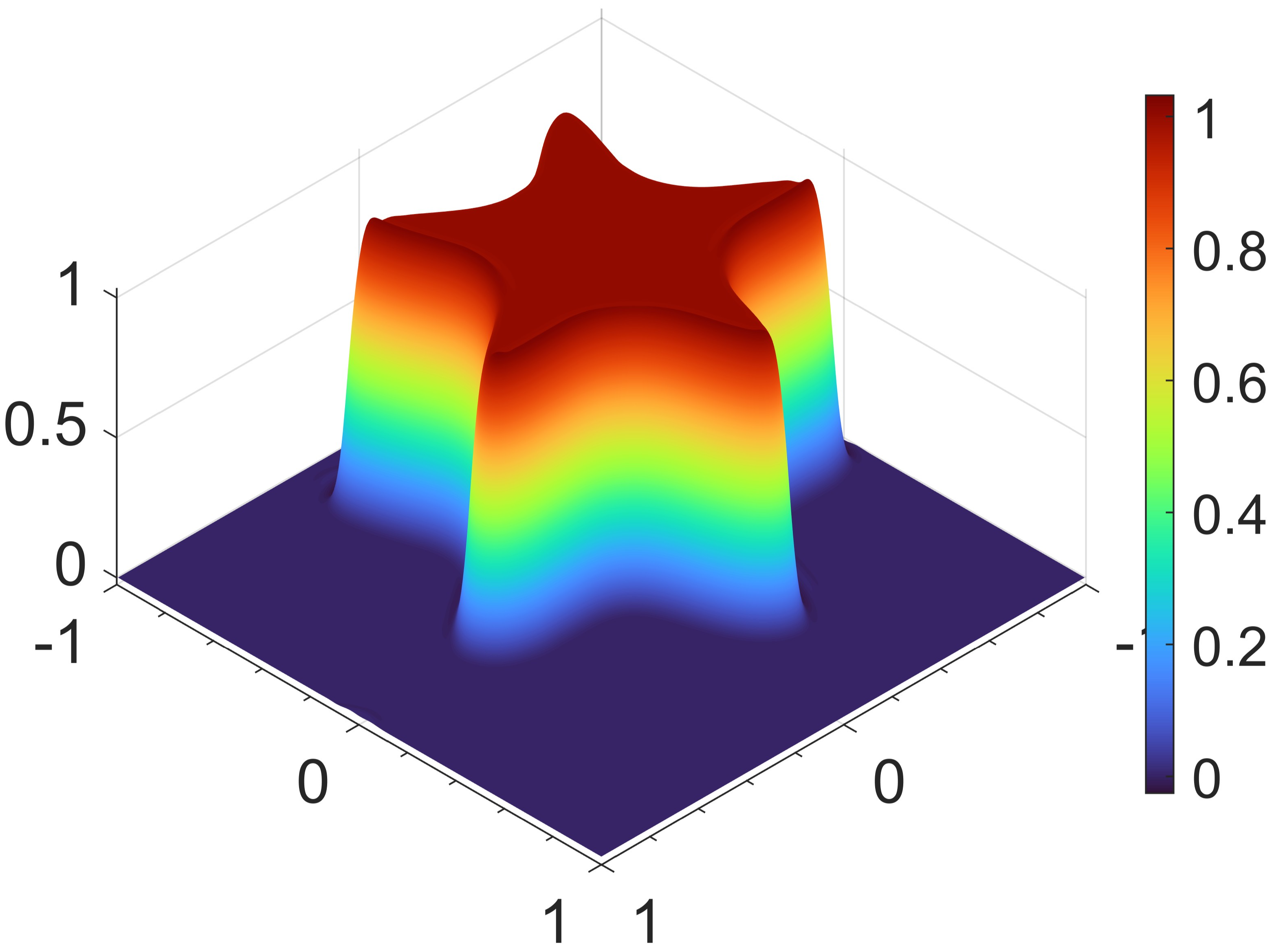
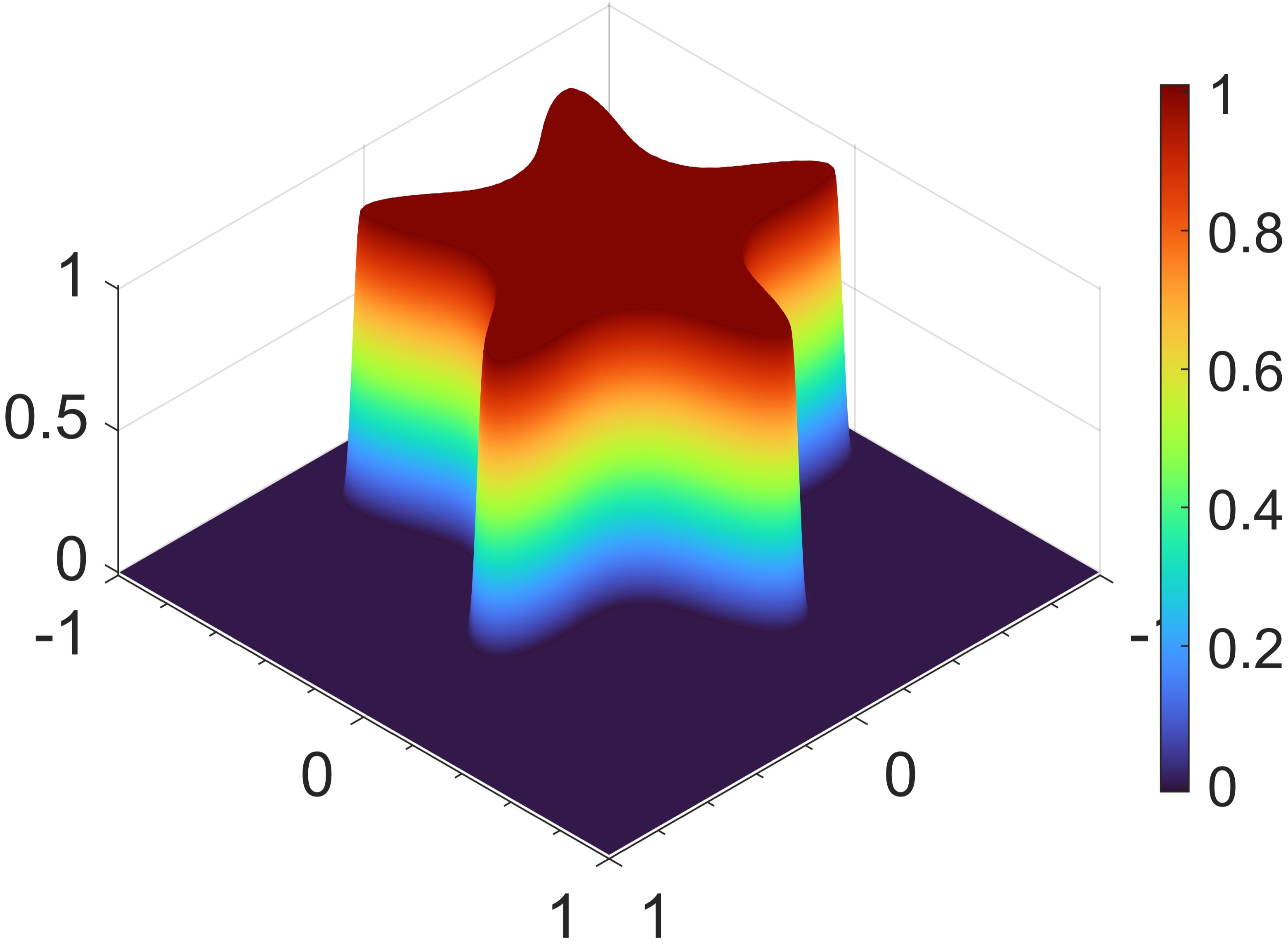
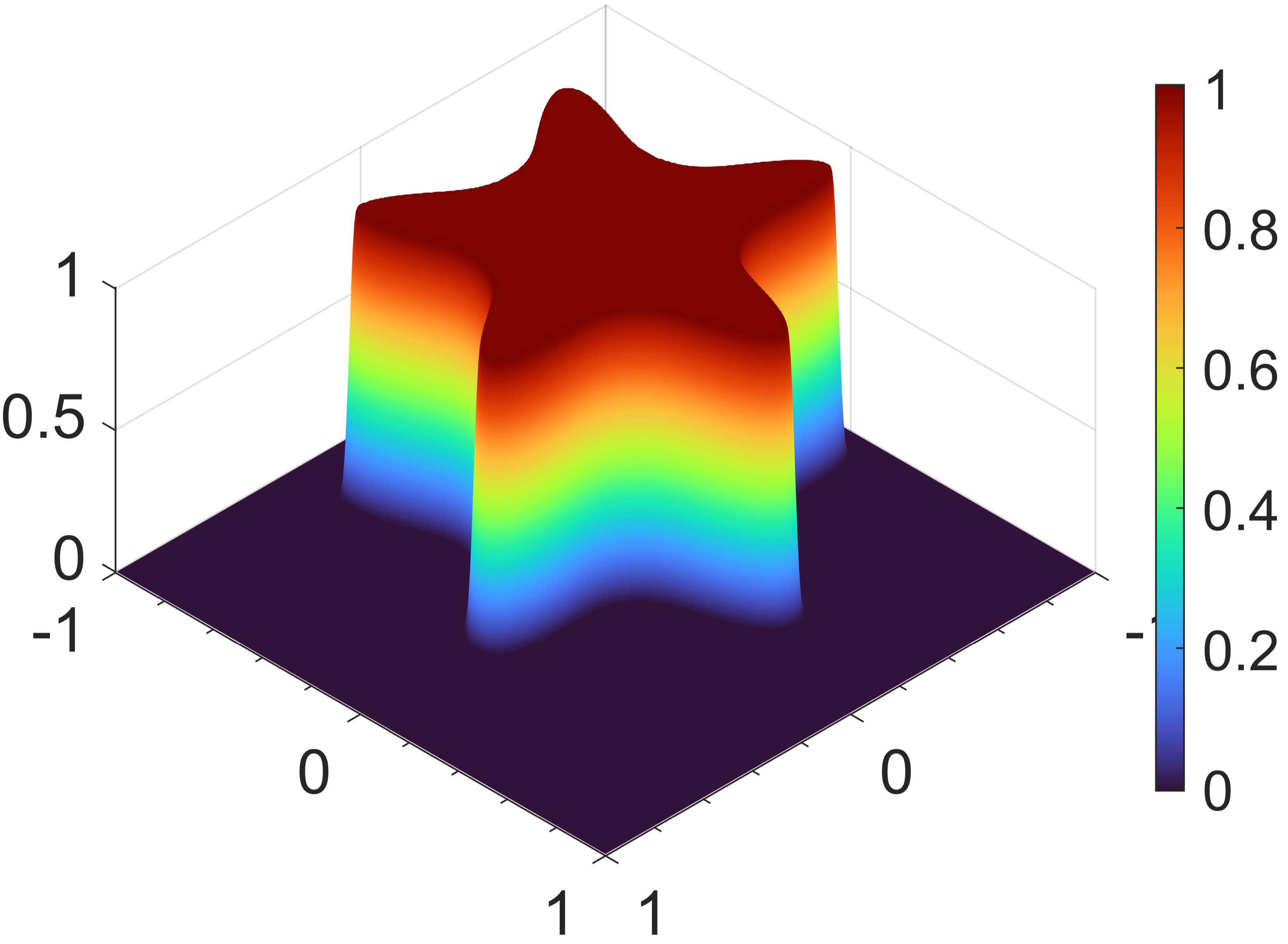
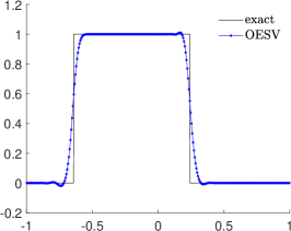
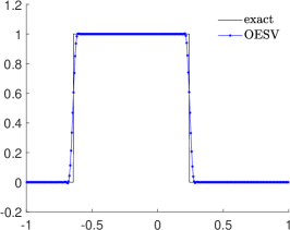
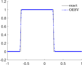
Figure 1: OESV solutions (top) at $t=1.8$ and their cut along $y=-0.25$ (bottom) for 2. From left to right: $\mathbb{Q}^{1}$, $\mathbb{Q}^{2}$, and $\mathbb{Q}^{3}$ approximations.

5.2 1D compressible Euler equations

This subsection presents several examples of the 1D compressible Euler equations ${\bf u}_{t}+{\bf f}({\bf u})_{x}={\bf 0}$ with ${\bf u}=(\rho,\rho v,E)^{\top}$ and ${\bf f}({\bf u})=(\rho v,\rho v^{2}+p,(E+p)v)^{\top}$, where $\rho$ is the density, $v$ is the velocity, $p$ is the pressure, and $E=\frac{p}{\gamma-1}+\frac{1}{2}\rho v^{2}$ represents the total energy. The adiabatic index is taken as $\gamma=1.4$ unless otherwise stated.

Example 3 (Riemann problems).

This example considers two classical Riemann problems for the 1D Euler equations. The first is the Sod problem with the initial conditions $(\rho_{0},v_{0},p_{0})=(1,~{}0,~{}1)$ for $x<0$ and $(0.125,~{}0,~{}0.1)$ for $x>0$. The second is the Lax problem with $(\rho_{0},v_{0},p_{0})=(0.445,~{}0.698,~{}3.528)$ for $x<0$ and $(0.5,~{}0,~{}0.571)$ for $x>0$. For both cases, we take the domain $\Omega=[-5,5]$ with outflow boundary conditions and conduct the simulation up to $t=1.3$. Fig. 2 presents the numerical solutions to the two Riemann problems computed by the $\mathbb{P}^{2}$-based OESV scheme with $256$ uniform cells. We observe that the OESV scheme captures the shock and the contact discontinuity effectively and suppresses spurious oscillations.

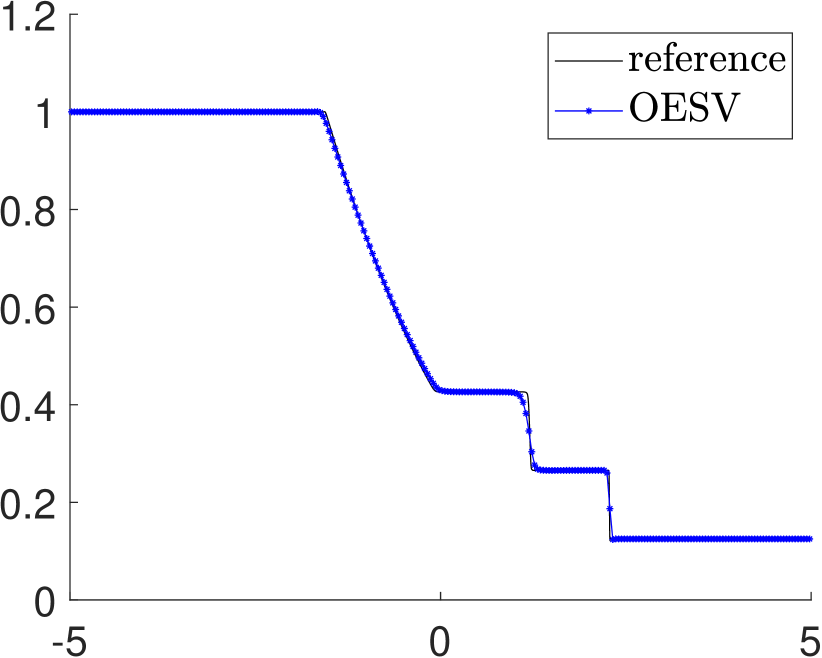
(a) Sod’s problem

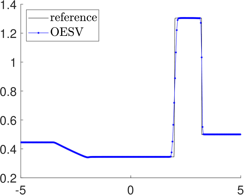
(b) Lax’s problem

Figure 2: Densities of two Riemann problems at $t=1.3$ computed by OESV scheme.

Example 4 (Blast problems).

This example simulates two blast problems. The first is the interaction of two blast waves proposed by Woodward and Colella. The spatial domain is $\Omega=[0,1]$ with reflective boundary conditions. The initial solution $(\rho_{0},v_{0},p_{0})$ is defined as $(1,0,10^{3})$ for $0<x<0.1$, as $(1,0,10^{-2})$ for $0.1<x<0.9$, and as $(1,0,10^{2})$ for $0.9<x<1$. Fig. 3(a) shows the numerical results at $t=0.038$ computed by the $\mathbb{P}^{2}$-based OESV scheme on a uniform mesh of $640$ cells. The reference solution is obtained using the $\mathbb{P}^{2}$-based OEDG scheme [22] with $10000$ uniform cells. As shown in Fig. 3(a), no spurious oscillations are observed near the discontinuities.

In the second test case, we investigate the Sedov blast problem on the domain $\Omega=[-2,2]$. This problem models the expanding wave caused by an intense explosion in a perfect gas, involving shocks and extremely low pressure. The initial conditions are $(\rho_{0},v_{0},E_{0})=(1,0,10^{-12})$ for all cells except the center one, which is initialized with $(\rho_{0},v_{0},E_{0})=(1,0,3200000/h)$, where $h$ denotes the uniform mesh size. We simulate this problem up to $t=0.001$ using the $\mathbb{P}^{2}$-based OESV scheme on a uniform mesh with 129 cells. It is worth mentioning that we do not apply any positivity-preserving limiter. The numerical results are presented in Fig. 3(b). The OESV scheme provides a satisfactory simulation without spurious oscillations, indicating its good robustness.

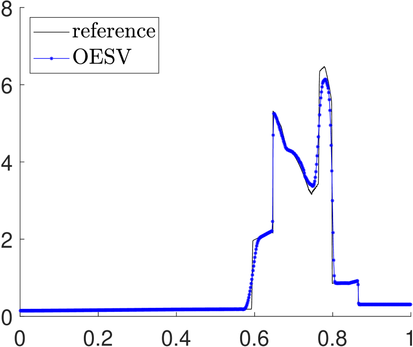
(a) Woodward–Colella blast wave,  $t=0.038$

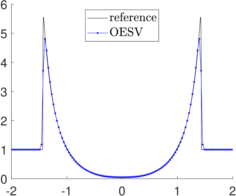
(b) Sedov blast,  $t=0.001$

Figure 3: Densities of 4 computed by the OESV scheme.

5.3 2D compressible Euler equations

This subsection presents several benchmark test cases of the 2D Euler equations, which can be written in the form of (2) with ${\bf u}=(\rho,\rho{\bf v},E)$ and $\quad{\bf f}({\bf u})=(\rho{\bf v},\rho{\bf v}\otimes{\bf v}+p{\bf I},(E+p){\bf v})$. Here, $\rho$ is the density, ${\bf v}$ represents the velocity field, $p$ is the pressure, and $E=\frac{p}{\gamma-1}+\frac{1}{2}\rho|{\bf v}|^{2}$ denotes the total energy. Unless otherwise specified, we set the adiabatic index $\gamma=1.4$.

Example 5 (double Mach reflection).

The double Mach reflection problem is a classical test case for assessing the capabilities of numerical schemes in handling strong shocks and their interactions. This problem describes a Mach 10 that initially forms an angle of $60^{\circ}$ relative to the bottom boundary of the spatial domain $\Omega=[0,4]\times[0,1]$. The initial conditions are defined as:

$$(\rho_{0},u_{0},v_{0},p_{0})=\begin{cases}(8,8.25\cos(\frac{\pi}{6}),-8.25\sin(\frac{\pi}{6}),116.5),\quad&x<\frac{1}{6}+\frac{y}{\sqrt{3}},\\ (1.4,0,0,1),\quad&x>\frac{1}{6}+\frac{y}{\sqrt{3}}.\end{cases}$$

The inflow boundary conditions are applied on the left boundary, and the outflow boundary conditions are applied on the right boundary. For the upper boundary, the postshock condition is imposed in the segment from $x=0$ to $x=\frac{1}{6}+\frac{1}{\sqrt{3}}(1+20t)$, while the preshock condition is used for the remaining part. For the lower boundary, the postshock condition holds from $x=0$ to $x=1/6$, and the reflective boundary condition is applied to the rest. The numerical solution is computed by the 2D $\mathbb{Q}^{2}$-based OESV scheme on a uniform rectangular mesh with $h_{x}=h_{y}=1/480$. Fig. 4 displays the density contours of the numerical solution at $t=0.2$. The result shows that the proposed OESV scheme resolves the flow structure clearly and eliminates nonphysical oscillations effectively.

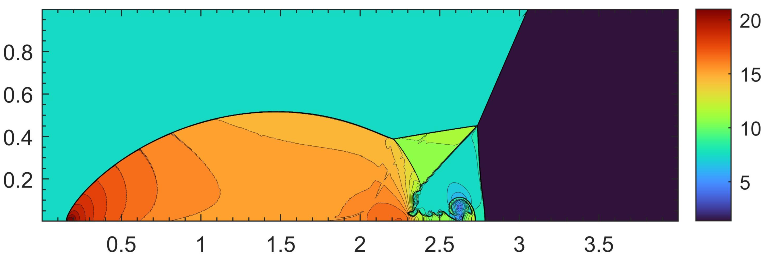
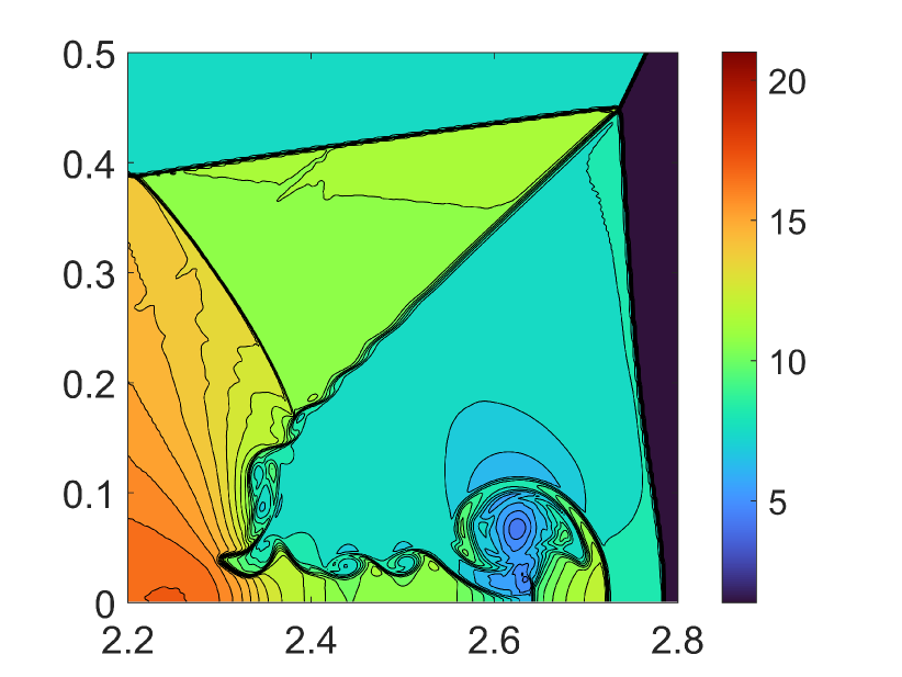
Figure 4: The contour plot of density (left) and its close-up (right) at $t=0.2$ obtained by the $\mathbb{Q}^{2}$-based OESV scheme with $h_{x}=h_{y}=1/480$.

Example 6 (Mach 2000 jet).

This example simulates a challenging jet problem in the spatial domain $\Omega=[0,1]\times[-0.25,0.25]$ to demonstrate the effectiveness of the proposed OESV scheme. The ratio of heat capacity is set to $\gamma=\frac{5}{3}$. Initially, $\Omega$ is full of a stationary fluid characterized by $(\rho,{\bf v},p)=(0.5,0,0,0.4127)$. A Mach-$2000$ jet with the state $(\rho,{\bf v},p)=(5,800,0,0.4127)$ is injected into $\Omega$ from the left boundary within the range $y=-0.05$ to $0.05$. The remaining boundaries are imposed with the outflow boundary conditions. We simulate the jet using the $\mathbb{Q}^{2}$-based OESV scheme with $320\times 160$ uniform cells. The numerical results at $t=0.001$ are displayed in Fig. 5. We observe that the proposed OESV scheme successfully captures the intricate structures of the jet flow, including the bow shock and the shear layer, and does not procedure any obvious spurious oscillations.

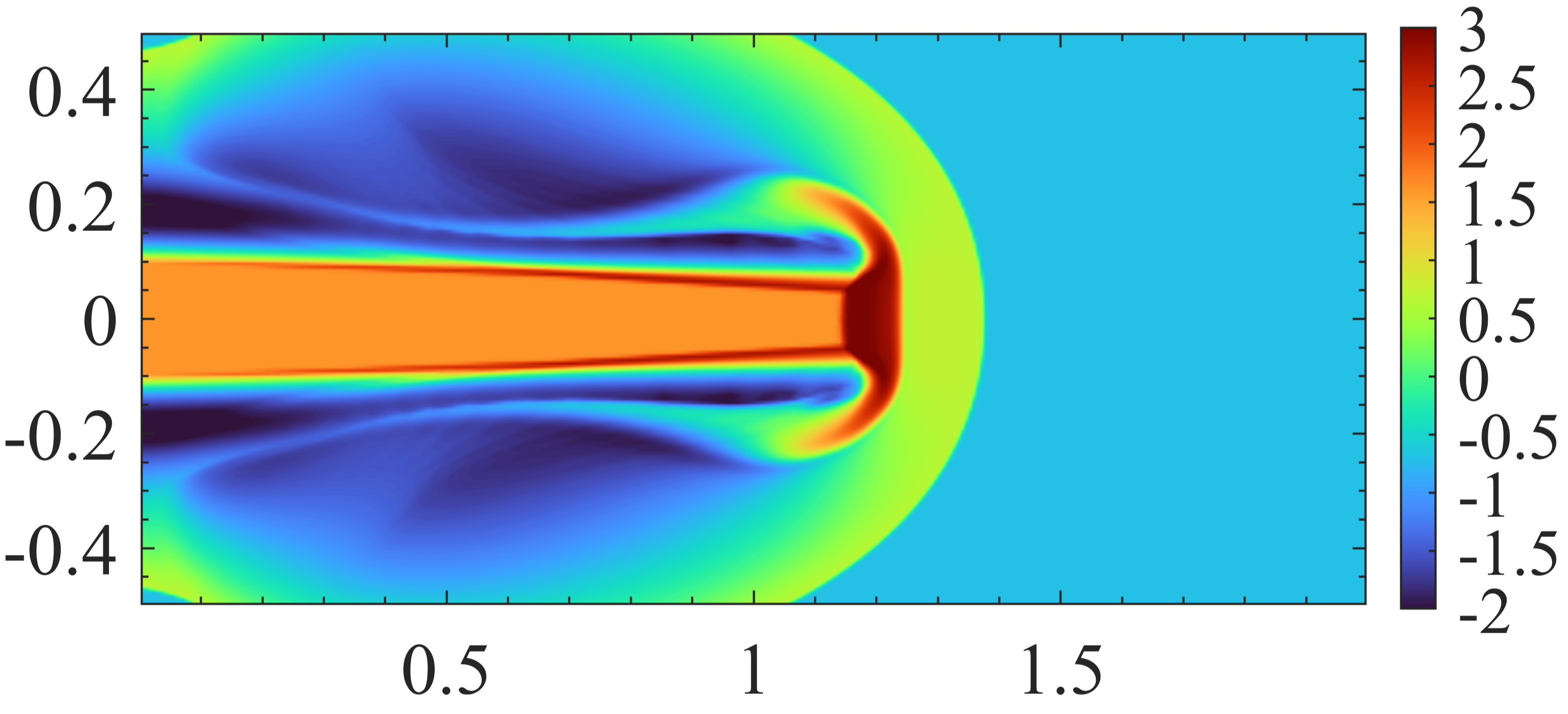
(a) Density logarithm

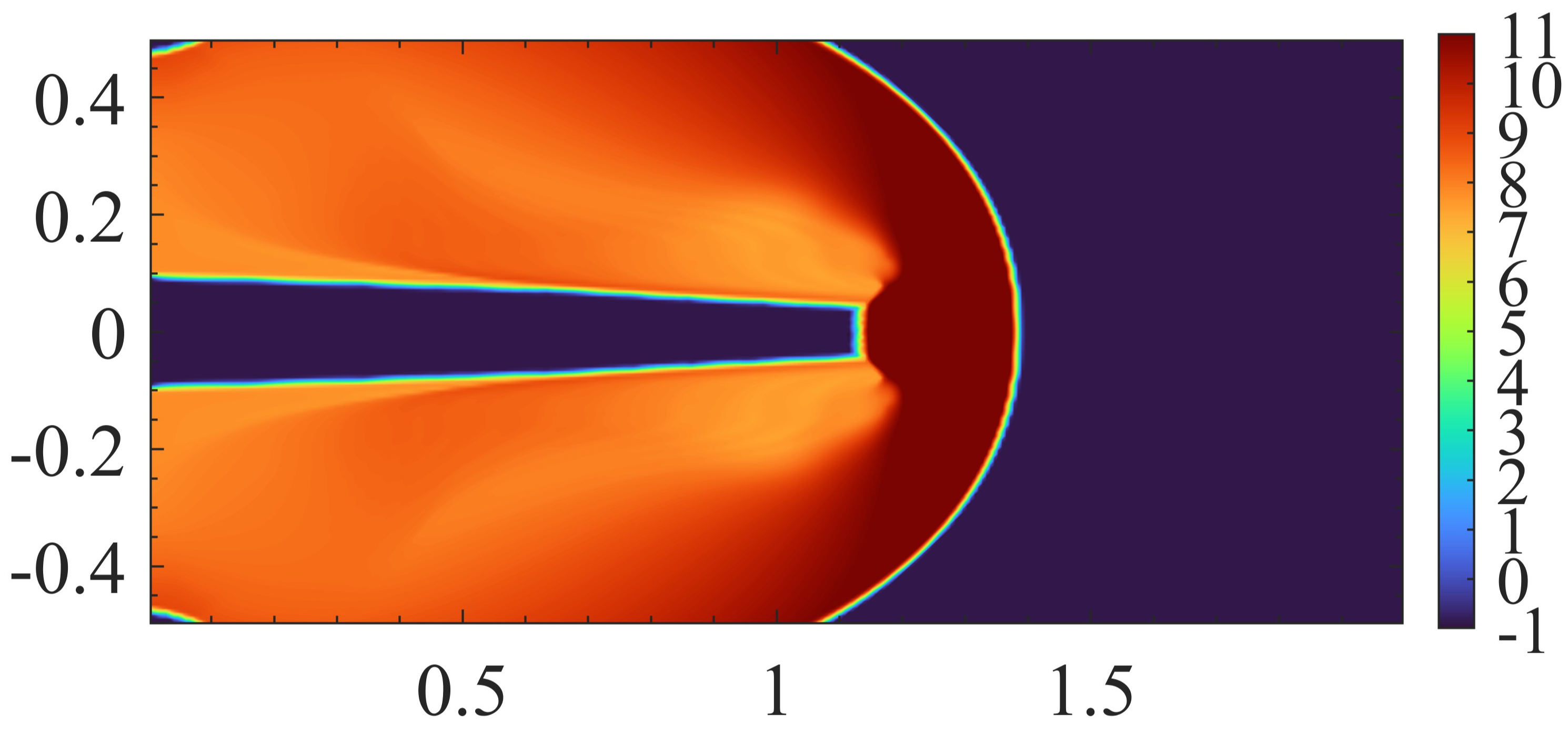
(b) Pressure logarithm

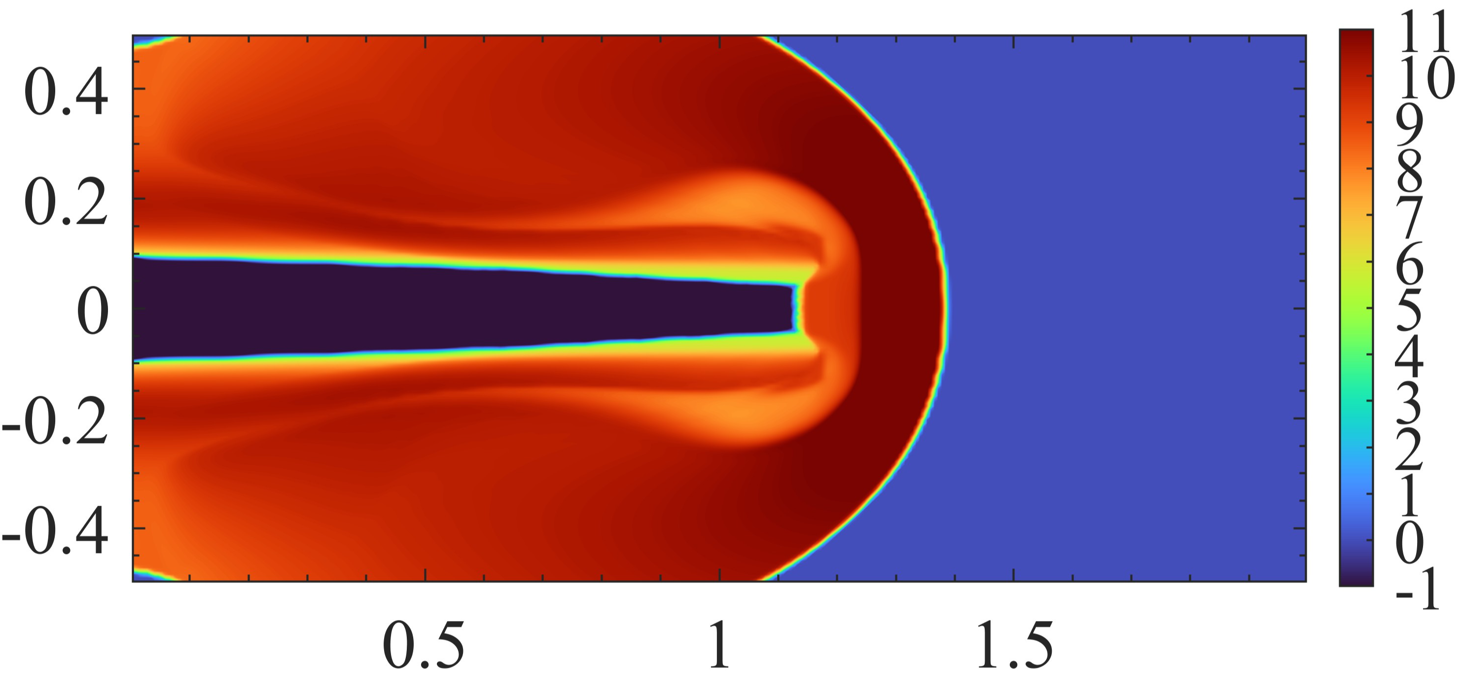
(c) Temperature logarithm

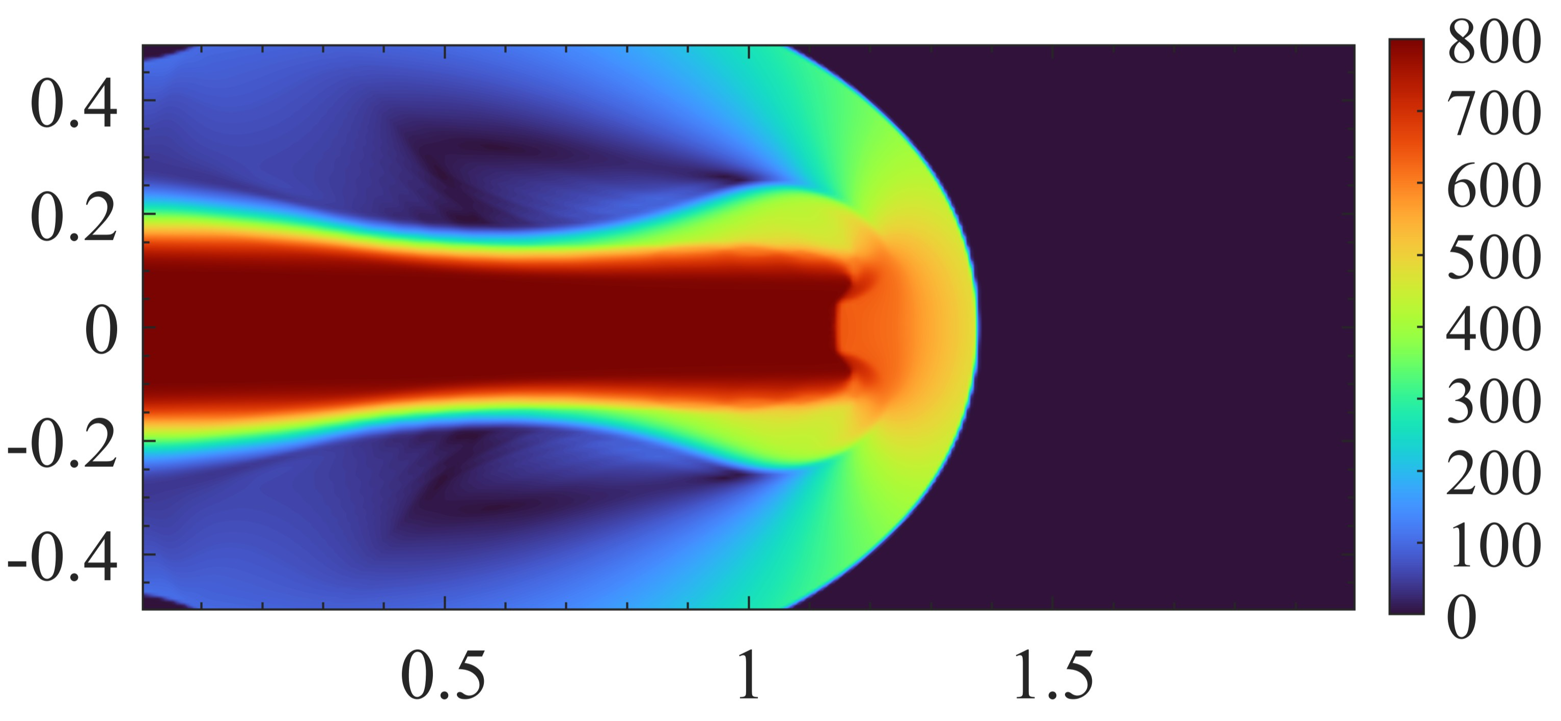
(d) Velocity magnitude

Figure 5: Numerical results at $t=0.001$ for the Mach 2000 jet problem.

Additional numerical examples can be found in Section 7.1.

6 Conclusions

In this paper, we have established a novel connection between the spectral volume (SV) method and the discontinuous Galerkin (DG) method for solving hyperbolic conservation laws, inspired by the Galerkin form of the SV method [5]. By demonstrating that the SV method can be represented in a DG form with a distinct inner product under specific subdivision assumptions, we have provided a unifying perspective for these two widely-used numerical methodologies. This insight allowed us to successfully extend the oscillation-eliminating (OE) technique, proposed by Peng, Sun, and Wu [22], to develop a new fully-discrete oscillation-eliminating SV (OESV) method. The OE procedure, being non-intrusive, efficient, and straightforward to implement, serves as a robust post-processing filter that effectively suppresses spurious oscillations. Our comprehensive framework, grounded in a DG perspective, facilitates rigorous theoretical analysis of the stability and accuracy of both general Runge–Kutta SV (RKSV) schemes and the novel OESV method. Specifically, for the linear advection equation, we identified a crucial upwind condition for stability and established optimal error estimates for the OESV schemes. The challenges arising from the nonlinearity of the OESV method were addressed through error decomposition and by treating the OE procedure as additional source terms in the RKSV schemes. Extensive numerical experiments have validated our theoretical analysis, demonstrating the effectiveness and robustness of the proposed OESV method across a range of benchmark problems. In conclusion, this work not only enhances the theoretical understanding of SV schemes but also significantly improves their practical application. It opens opportunities for future research to explore further extensions and applications of the OESV method for high-resolution simulations of various complex hyperbolic systems.

7 Appendix

This appendix provides some additional numerical examples and the proofs of several auxiliary propositions.

7.1 Additional numerical examples

Example 7 (smooth problem).

This example examines a smooth problem of the 1D compressible Euler equations on the spatial domain $\Omega=[0,2\pi]$ with the periodic boundary conditions. The exact solution is given by $\rho(x,t)=2+2\sin^{2}(x-t)$, $v(x,t)=1$, and $p(x,t)=2$. The problem is simulated up to $t=1.1$ using the $\mathbb{P}^{k}$-based OESV scheme with a CFL number $C_{\mathrm{CFL}}=\frac{0.95}{2k+1}$. The errors and corresponding convergence rates are listed in Table 2. It is observed that the $\mathbb{P}^{k}$-based OESV scheme achieves the optimal convergence rate of $(k+1)$th-order for this problem.

Table 2: Errors and convergence rates for $\mathbb{P}^{k}$-based OESV scheme for 1D Euler equations.

$k$	$N_{x}$	$L^{1}$ error	rate	$L^{2}$ error	rate	$L^{\infty}$ error	rate
$1$	256	1.62e-03	-	7.70e-04	-	6.24e-04	-
	512	2.92e-04	2.47	1.38e-04	2.48	1.14e-04	2.46
	1024	6.65e-05	2.13	2.99e-05	2.21	2.35e-05	2.27
	2048	1.60e-05	2.05	7.15e-06	2.07	5.44e-06	2.11
	4096	3.95e-06	2.02	1.77e-06	2.02	1.34e-06	2.02
	8192	9.83e-07	2.01	4.40e-07	2.00	3.34e-07	2.00
	16384	2.45e-07	2.00	1.10e-07	2.00	8.36e-08	2.00
	32768	6.12e-08	2.00	2.75e-08	2.00	2.09e-08	2.00
$2$	256	8.44e-06	-	4.28e-06	-	4.24e-06	-
	512	7.68e-07	3.46	4.03e-07	3.41	4.17e-07	3.35
	1024	9.00e-08	3.09	4.55e-08	3.15	4.74e-08	3.14
	2048	1.10e-08	3.03	5.49e-09	3.05	5.71e-09	3.05
	4096	1.37e-09	3.01	6.77e-10	3.02	7.04e-10	3.02
	8192	1.70e-10	3.01	8.41e-11	3.01	8.81e-11	3.00
$3$	256	1.77e-08	-	8.17e-09	-	7.20e-09	-
	512	6.32e-10	4.81	2.99e-10	4.77	3.00e-10	4.59
	1024	2.89e-11	4.45	1.36e-11	4.46	1.41e-11	4.41
	2048	1.53e-12	4.24	7.50e-13	4.18	8.70e-13	4.02

Example 8 (smooth problem).

This example serves as an accuracy test for the 2D $\mathbb{Q}^{k}$-based OESV scheme for the linear advection equation:

(79) $$u_{t}+u_{x}+u_{y}=0,\quad(x,y)\in\Omega=[0,1]\times[0,1],$$

with the periodic boundary conditions. The simulation is initialized with $u_{0}(x,y)=\sin^{2}\left(\pi(x+y)\right)$. We list the numerical errors on a mesh of $N_{x}\times N_{y}$ cells at $t=1.1$ and the corresponding convergence rates in Table 3. On coarse meshes, it is observed that the high-order damping effect dominates the numerical errors, leading to convergence rates exceeding $k+1$. This effect was also observed in the OEDG method [22].

Table 3: Errors and convergence rates of 2D $\mathbb{Q}^{k}$-based OESV scheme for 8.

$k$	$N_{x}\times N_{y}$	$L^{1}$ error	rate	$L^{2}$ error	rate	$L^{\infty}$ error	rate
$1$	$80\times 64$	2.18e-02	-	2.58e-02	-	4.32e-02	-
	$160\times 128$	3.68e-03	2.57	4.32e-03	2.58	7.07e-03	2.61
	$320\times 256$	6.19e-04	2.57	7.23e-04	2.58	1.23e-03	2.52
	$640\times 512$	1.16e-04	2.41	1.31e-04	2.47	2.37e-04	2.38
	$1280\times 1024$	2.54e-05	2.20	2.78e-05	2.24	4.80e-05	2.30
	$2560\times 2048$	5.97e-06	2.09	6.54e-06	2.09	1.05e-05	2.20
$2$	$80\times 64$	6.49e-04	-	7.43e-04	-	1.16e-03	-
	$160\times 128$	2.31e-05	4.82	2.57e-05	4.85	3.74e-05	4.95
	$320\times 256$	1.23e-06	4.23	1.35e-06	4.25	1.92e-06	4.28
	$640\times 512$	7.81e-08	3.98	8.46e-08	3.99	1.18e-07	4.03
	$1280\times 1024$	5.66e-09	3.79	6.07e-09	3.80	8.20e-09	3.85
	$2560\times 2048$	4.68e-10	3.60	5.00e-10	3.60	6.51e-10	3.65
$3$	$80\times 64$	4.82e-06	-	5.64e-06	-	9.79e-06	-
	$160\times 128$	1.65e-07	4.87	1.86e-07	4.92	3.16e-07	4.95
	$320\times 256$	5.26e-09	4.97	5.89e-09	4.98	9.48e-09	5.06
	$640\times 512$	1.67e-10	4.98	1.86e-10	4.99	2.89e-10	5.04
	$1280\times 1024$	5.24e-12	4.99	5.83e-12	4.99	8.48e-12	5.09

Example 9 (2D smooth problem).

The exact solution of this example is smooth, describing a sine wave periodically propagating in the spatial domain $\Omega=[0,2]\times[0,2]$, and given by $(\rho,{\bf v},p)=(1+0.2\sin(\pi(x+y-t)),0.7,0.3,1)$. We compute the numerical solution using the 2D $\mathbb{Q}^{k}$-based OESV scheme. The numerical errors and the corresponding convergence rates for the density at $t=2$ are presented in Table 4. We observe the expected convergence rate of $k+1$ for the $\mathbb{Q}^{k}$-based OESV scheme.

Table 4: Errors and convergence rates for 2D $\mathbb{Q}^{k}$-based OEDG method for 9.

	$N_{x}\times N_{y}$	$L^{1}$ error	rate	$L^{2}$ error	rate	$L^{\infty}$ error	rate
$1$	80$\times$80	2.14e-04	-	2.38e-04	-	3.38e-04	-
	160$\times$160	5.36e-05	2.00	5.95e-05	2.00	8.42e-05	2.00
	320$\times$320	1.34e-05	2.00	1.49e-05	2.00	2.10e-05	2.00
	640$\times$640	3.35e-06	2.00	3.72e-06	2.00	5.26e-06	2.00
	1280$\times$1280	8.37e-07	2.00	9.29e-07	2.00	1.31e-06	2.00
$2$	80$\times$80	5.71e-08	-	6.90e-08	-	1.55e-07	-
	160$\times$160	6.06e-09	3.24	8.33e-09	3.05	2.05e-08	2.92
	320$\times$320	2.24e-10	4.76	2.65e-10	4.97	5.59e-10	5.20
	640$\times$640	2.04e-11	3.46	2.58e-11	3.36	6.01e-11	3.22
	1280$\times$1280	2.60e-12	2.97	3.31e-12	2.96	8.47e-12	2.83
$3$	80$\times$80	8.93e-10	-	1.14e-09	-	2.75e-09	-
	160$\times$160	4.66e-11	4.26	6.03e-11	4.24	1.47e-10	4.23
	320$\times$320	1.77e-12	4.72	2.29e-12	4.72	6.59e-12	4.48
	640$\times$640	9.08e-14	4.28	1.07e-13	4.42	2.22e-13	4.89

Example 10 (shock reflection problem).

This example simulates the shock reflection problem [48] for the 2D compressible Euler equations in the spatial domain $\Omega=[0,4]\times[0,1]$. The initial conditions for this problem are defined as $(\rho_{0},{\bf v}_{0},p_{0})=(1,2.9,0,\frac{5}{7}),$, which are also applied as the inflow boundary conditions on the left boundary of $\Omega$. On the upper boundary of $\Omega$, a different set of inflow boundary conditions is applied:

$$(\rho,{\bf v},p)=(1.69997,2.61934,-0.50632,1.52819).$$

Reflective wall boundary conditions are applied on the lower boundary of $\Omega$, while the right boundary is subjected to outflow boundary conditions.

The numerical solution for this example is obtained using the 2D $\mathbb{Q}^{2}$-based OESV scheme on a uniform rectangular mesh of $200\times 50$ cells. Following [17], we compute the average residue to study the convergence behavior of the numerical solution. The average residue is defined as:

(80) $${\rm Res}:=\frac{1}{4N_{x}N_{y}}\sum_{i=1}^{N_{x}}\sum_{j=1}^{N_{y}}\sum_{q=1}^{4}\left|R^{(q)}_{ij}\right|,$$

where $R^{(q)}_{ij}:=\frac{1}{\tau}(u_{h}^{n+1,(q)}-u_{h}^{n,(q)})$ is the local residue on the cell $[x_{i-\frac{1}{2}},x_{i+\frac{1}{2}}]\times[y_{j-\frac{1}{2}},y_{j+\frac{1}{2}}]$, and $u_{h}^{n,(q)}$ represents the $q$th component of the numerical solution at the $n$th time step.

We plot the logarithm of the average residue over time in Fig. 6(a). The plot shows that the average residue decreases to the level of machine error in double precision after about $t=9$, indicating that the numerical solution converges to a steady state as time progresses. The density contour of the numerical solution at $t=20$ is displayed in Fig. 6(b), where the shock waves are clearly captured without spurious oscillations.

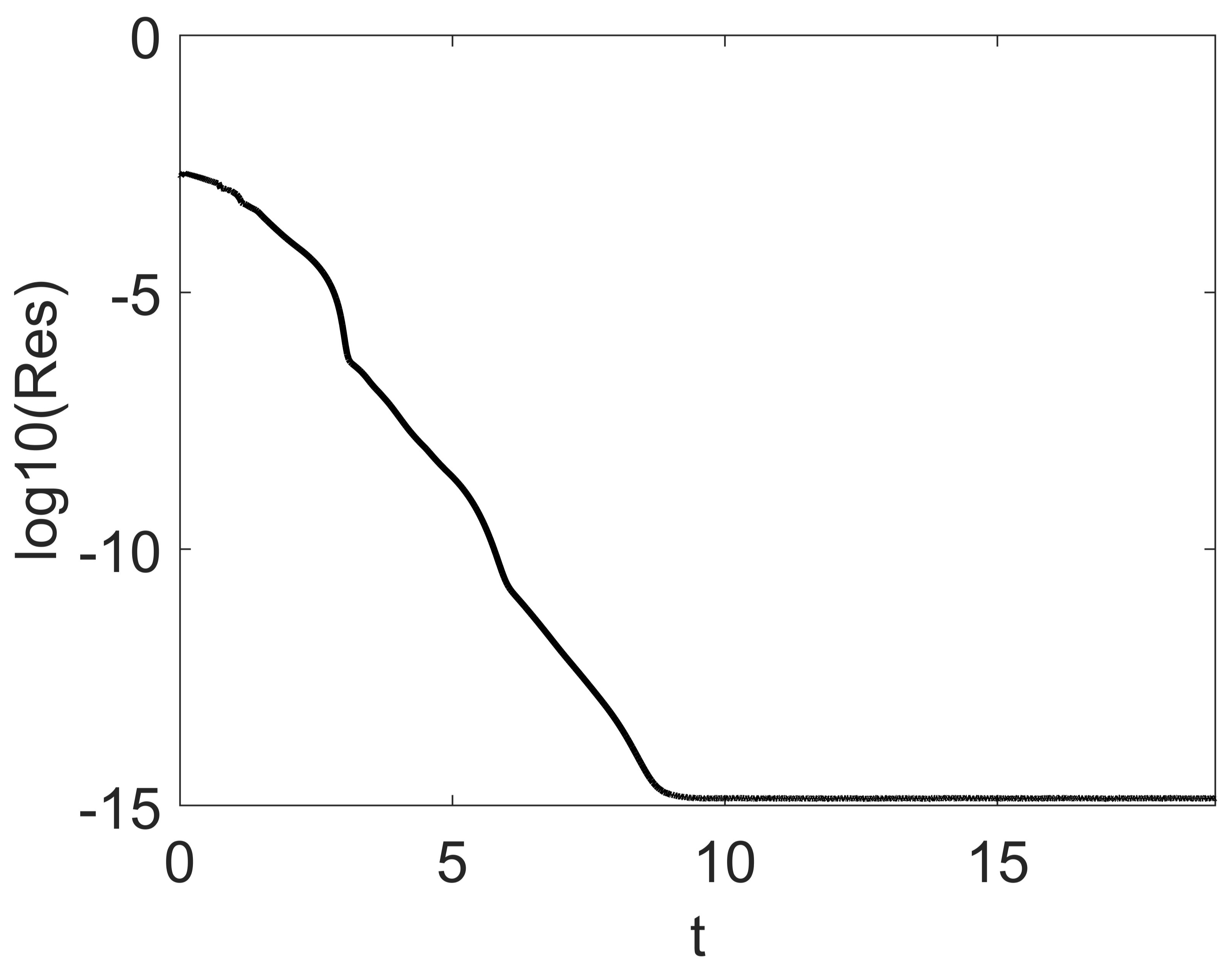
(a) Average residue

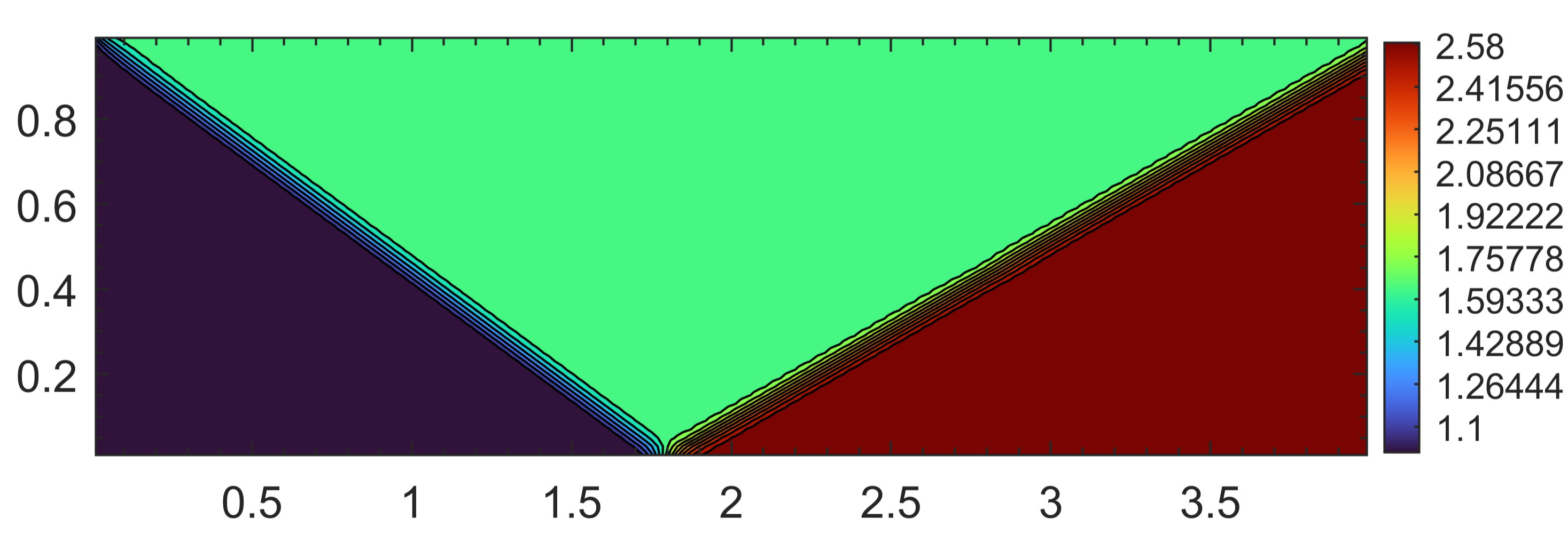
(b) Density contour at $t=20$

Figure 6: Shock reflection problem simulated by $\mathbb{Q}^{2}$-based OESV scheme.

Example 11 (supersonic flow past two plates).

This example [49] simulates a supersonic flow in the spatial domain $\Omega=[0,10]\times[-5,5]$ with the initial conditions $(\rho_{0},{\bf v}_{0},p_{0})=\left(1,\cos(\frac{\pi}{12}),\sin(\frac{\pi}{12}),\frac{1}{\gamma M_{\infty}^{2}}\right),$ where $M_{\infty}=3$ is the Mach number of the free stream. The supersonic flow pasts two plates with an attack angle of $15^{\circ}$. The two plates are placed at $y=\pm 2$ with $x\in(2,3)$, and slip boundary conditions are applied on both plates. The inflow boundary conditions are applied on the left and lower boundaries of $\Omega$. The outflow boundary conditions are applied on the upper and right boundaries. The simulation is performed using the 2D $\mathbb{Q}^{2}$-based OESV scheme on a mesh of $200\times 200$ uniform cells. Similar to 10 and [22], we display the average residue history and plot the density contour of the numerical solution at $t=100$ in Fig. 7. One can see from Fig. 7(a) that the numerical solution reaches a steady state at $t=100$. We also observe from Fig. 7(b) that the OESV scheme captures the flow structure correctly with no nonphysical oscillations.

(a) Average residue

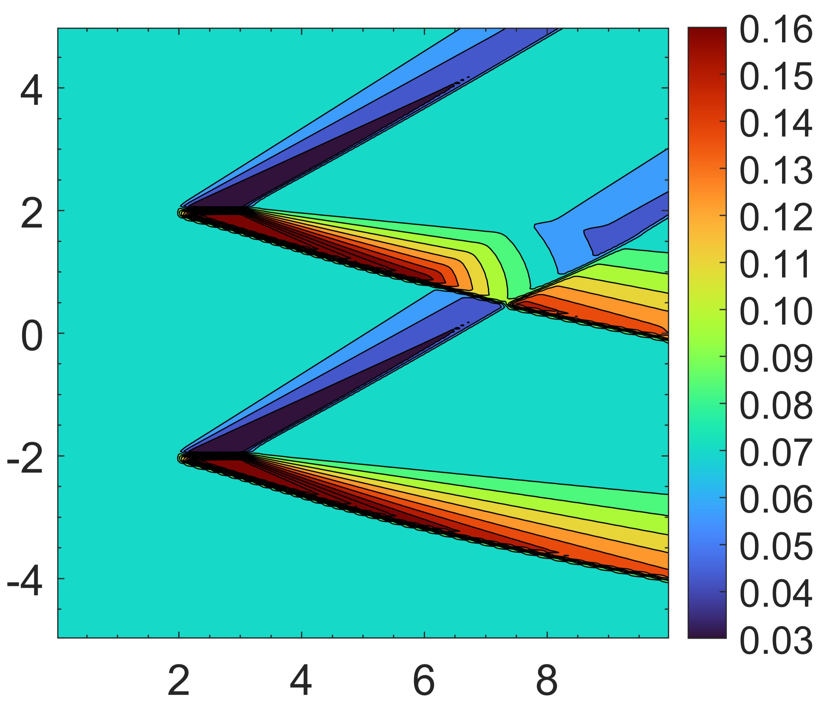
(b) Density contour at $t=100$

Figure 7: Supersonic flow problem simulated by $\mathbb{Q}^{2}$-based OESV scheme.

Example 12 (shock-vortex interaction).

We consider the interaction between a vortex and a Mach 1.1 shock in the spatial domain $\Omega=[0,2]\times[0,1]$ by solving the 2D compressible Euler equations. The shock is perpendicular to the $x$-axis and is positioned at $x=0.5$, with the left upstream state $(\rho,{\bf v},p)=(1,1.1\sqrt{\gamma},0,1)$. At $t=0$, an isentropic vortex centered at $(x_{c},y_{c})=(0.25,0.5)$ is added to the mean flow. The velocity, temperature, and entropy perturbations due to the vortex are defined by

$$\delta{\bf v}=\frac{\varepsilon}{r_{c}}e^{\alpha(1-\eta^{2})}(\bar{y},-\bar{x}),\quad\delta T=-\frac{(\gamma-1)\varepsilon^{2}}{4\alpha\gamma}e^{2\alpha(1-\eta^{2})},\quad\delta S=0,$$

where $r^{2}=\bar{x}^{2}+\bar{y}^{2}$, $\eta=\frac{r}{r_{c}}$, and $(\bar{x},\bar{y})=(x-x_{c},y-y_{c})$. $\varepsilon=0.3$ is the strength of the vortex, $\alpha=0.204$ denotes the decay rate of the vortex, and $r_{c}=0.05$ represents the critical radius of the vortex. The inflow boundary conditions are applied on the left boundary and the outflow boundary conditions are imposed on the right boundary. Meanwhile, reflective boundary conditions are applied on both the upper and lower boundaries.

We divide $\Omega$ into $400\times 200$ uniform rectangular cells and conduct the simulation using the 2D $\mathbb{Q}^{2}$-based OESV scheme up to $t=0.8$. Fig. 8 presents the pressure contour plots of the numerical solution at six different time instances. The results obtained by the proposed OESV scheme match well with those reported in [17], without producing any nonphysical oscillations.

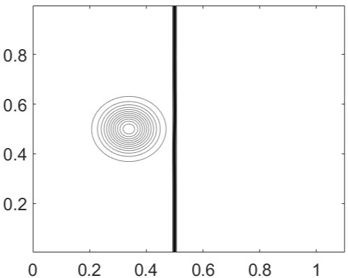
(a) $t=0.068$

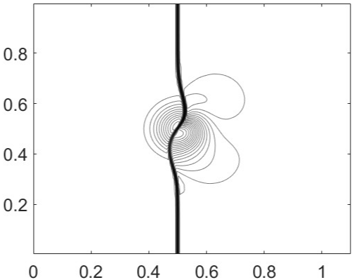
(b) $t=0.203$

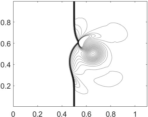
(c) $t=0.330$

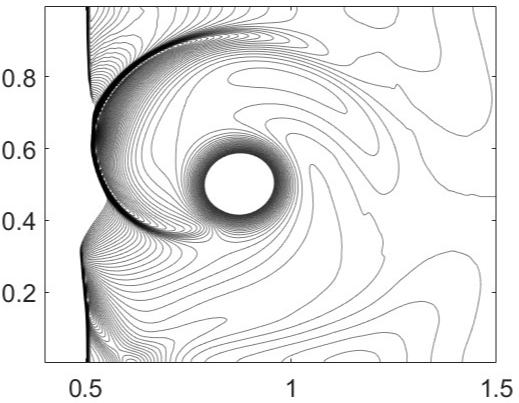
(d) $t=0.529$

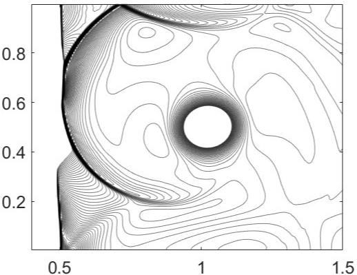
(e) $t=0.662$

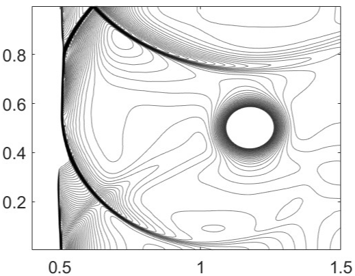
(f) $t=0.8$

Figure 8: Contour plots of pressure for shock-vortex interaction: 50 contour lines from 0.68 to 1.3 are shown in the top figures, while 90 contour lines from 1.19 to 1.36 are plotted in the bottom figures.

7.2 Proof of Proposition 3.3

If $k=0$, then $\mathbb{V}^{k,*}=\mathbb{V}^{k}$ and $M^{*}\omega=\omega$ for all $\omega\in\mathbb{V}^{k}$. If $k\geq 1$, then for every $\omega^{*}\in\mathbb{V}^{k,*}$, we define $\omega_{i,j}^{*}$ as the constant value of $\omega^{*}$ on $I_{i,j}$. Then, we can find $p_{i}\in\mathbb{P}^{k-1}(I_{i})$ for each $i$ such that

$$p_{i}(x_{i,j})=\begin{cases}0,~{}~{}&\mbox{if}~{}A_{i,j}=0,\\ \frac{\omega_{i,j}^{*}-\omega_{i,j-1}^{*}}{A_{i,j}},~{}~{}&\mbox{otherwise},\end{cases}\quad j=1,\dots,k.$$

Note that there exists $P_{i}\in\mathbb{P}^{k}(I_{i})$ such that $(P_{i})_{x}=p_{i}$ and $P_{i}(x_{i-\frac{1}{2}})=\omega_{i,0}^{*}-A_{i,0}p_{i}(x_{i-\frac{1}{2}})$. Hence, if we define $\omega\in\mathbb{V}^{k}$ by $\omega|_{I_{i}}=P_{i}$ for all $i$, then $\omega^{*}=M^{*}\omega$. The proof is completed.

7.3 Proof of Proposition 3.8

For any $\omega\in\mathbb{V}^{k}$, the Cauchy–Schwarz inequality and the definition of $Q_{i}^{k}$ imply

(81) $$\left\|M^{*}\omega\right\|^{2}\leq(k+1)\sum_{i}\left(h_{i}\left\|\omega\right\|_{L^{\infty}(I_{i})}^{2}+h_{i}^{2}Q_{i}^{k}(\omega_{x}^{2})\right).$$

Since $\omega_{x}^{2}|_{I_{i}}\in\mathbb{P}^{2k-1}(I_{i})$, we have $Q_{i}^{k}(\omega_{x}^{2})=\left\|\omega_{x}\right\|_{L^{2}(I_{i})}^{2}$. Applying inverse inequalities (33a) and (33b) to the right hand side of (81) completes the proof.

8 Proof of Proposition 3.10

Lemma 3.2 implies $\left(v,\omega\right)_{*}=\left(v,\omega\right)+\sum_{i}R_{i}^{k}(V\omega_{x})$ for some $V\in\mathbb{V}^{k+1}$. For $\omega\in\mathbb{V}^{k-1}$, $R_{i}^{k}(V\omega_{x})=0$ for all $i$, which implies (23). To prove (24), we take $C=1+\sqrt{\left\|M^{*}\right\|}$, and Proposition 3.8 indicates that

(82) $$\left\|v\right\|_{*}^{2}=\left(v,M^{*}v\right)\leq\left\|M^{*}\right\|\left\|v\right\|^{2}\leq\left(C\left\|v\right\|\right)^{2}.$$

Using (22) and (23), we can verify that $c\left\|v\right\|\leq\left\|v\right\|_{*}$ for any $v\in\mathbb{V}^{k}$, where

(83) $$c=\min\left\{1,\min_{i}\left\{1-(2k-1)\frac{Q_{i}^{k}(L_{i,k+1}L_{i,k-1})}{h_{i}}\right\}\right\}.$$

The constant $c>0$ is independent of the mesh $\{I_{i}\}$, since $\frac{Q_{i}^{k}}{h_{i}}$ is independent of $h_{i}$ ([2]).

8.1 Proof of the statement in Remark 4.2

Without the loss of generality, we assume that $g\equiv 0$ in (27). First, we observe from (10) and (23) that

(84) $$\left\|\mathcal{F}_{\tau}v\right\|_{*}\leq\left\|v\right\|_{*}\quad\forall v\in\mathbb{V}^{k}.$$

We will prove the statement in Remark 4.2 by induction for $\left\|u_{h}^{n,\ell+1}\right\|_{*}$.

For the OESV scheme (30), using (38) gives $u_{h}^{n,1}=\mathcal{F}_{\tau}\left(u_{h}^{n}+d_{00}\mathbb{D}^{*}u_{h}^{n}\right)$. Because $d_{00}\geq 0$, Proposition 4.9 and (84) yield that

(85) $$\left\|u_{h}^{n,1}\right\|_{*}^{2} \leq\left(u_{h}^{n}+d_{00}\mathbb{D}^{*}u_{h}^{n},u_{h}^{n}+d_{00}\mathbb{D}^{*}u_{h}^{n}\right)_{*}$$

$$\leq\left(1+d_{00}^{2}\left\|\mathbb{D}^{*}\right\|_{*}^{2}\right)\left\|u_{h}^{n}\right\|_{*}^{2}-d_{00}\llbracket u_{h}^{n}\rrbracket^{2}$$

$$\leq\left(1+C\left(\frac{\tau}{h}\right)^{2}\right)\left\|u_{h}^{n}\right\|_{*}^{2}\leq\left(1+C_{(0)}\tau\right)\left\|u_{h}^{n}\right\|_{*}^{2},$$

for some $C_{(0)}\geq 0$ if $\frac{\tau}{h^{2}}\leq C_{\mathrm{CFL}}^{*}$. Now suppose that $\left\|u_{h}^{n,\ell+1}\right\|_{*}^{2}\leq\left(1+C_{(\ell)}\tau\right)\left\|u_{h}^{n}\right\|_{*}^{2}$ for $0\leq\ell<\ell_{0}$ when $\frac{\tau}{h^{2}}\leq C_{\mathrm{CFL}}^{*}$. Because $d_{\ell_{0}\kappa}\geq 0$, similar to the derivation of (85), we can show that if $\frac{\tau}{h^{2}}\leq C_{\mathrm{CFL}}^{*}$, then

(86) $$\left\|u_{h}^{n,\kappa}+\frac{d_{\ell_{0}\kappa}}{c_{\ell_{0}\kappa}}\mathbb{D}^{*}u_{h}^{n,\kappa}\right\|_{*}^{2}\leq\left(1+C\tau\right)\left\|u_{h}^{n,\kappa}\right\|_{*}^{2}\leq\left(1+C\tau\right)\left\|u_{h}^{n}\right\|_{*}^{2},$$

for $0\leq\kappa\leq\ell_{0}$. Here, we set $\frac{d_{\ell_{0}\kappa}}{c_{\ell_{0}\kappa}}=1$ if $c_{\ell_{0}\kappa}=0$. Notice that (30) implies

$$u_{h}^{n,\ell_{0}+1}=\sum_{0\leq\kappa\leq\ell_{0}}c_{\ell_{0}\kappa}\left(u_{h}^{n,\kappa}+\frac{d_{\ell_{0}\kappa}}{c_{\ell_{0}\kappa}}\mathbb{D}^{*}u_{h}^{n,\kappa}\right).$$

As $c_{\ell_{0}\kappa}\geq 0$ and $\sum_{\kappa}c_{\ell_{0}\kappa}=1$, the convexity of the function $h(x)=x^{2}$ yields

(87) $$\left\|u_{h}^{n,\ell_{0}+1}\right\|_{*}^{2} \leq\left(\sum_{0\leq\kappa\leq\ell_{0}}c_{\ell_{0}\kappa}\left\|u_{h}^{n,\kappa}+\frac{d_{\ell_{0}\kappa}}{c_{\ell_{0}\kappa}}\mathbb{D}^{*}u_{h}^{n,\kappa}\right\|_{*}\right)^{2}$$

$$\leq\sum_{0\leq\kappa\leq\ell_{0}}c_{\ell_{0}\kappa}\left\|u_{h}^{n,\kappa}+\frac{d_{\ell_{0}\kappa}}{c_{\ell_{0}\kappa}}\mathbb{D}^{*}u_{h}^{n,\kappa}\right\|_{*}^{2}\leq\left(1+C_{(\ell_{0})}\tau\right)\left\|u_{h}^{n}\right\|_{*}^{2},$$

when $\frac{\tau}{h^{2}}\leq C_{\mathrm{CFL}}^{*}$. By (85) and (87), the desired result (35) for the OESV scheme (30) is then verified using mathematical induction.

8.2 Proof of Proposition 4.30

According to [22], we introduce the following notations:

$$\tilde{\xi}^{n,\ell+1}=\tilde{u}_{h}^{n,\ell+1}-\mathbf{P}U^{n,\ell+1},\quad\eta^{n,\ell+1}=U^{n,\ell+1}-\mathbf{P}U^{n,\ell+1}$$

where $\mathbf{P}$ denotes the Gauss–Radau projection. [22, Section 4.4.2] has shown that there exists a constant $h_{0}>0$ independent of $n$ and $\ell$ such that

(88) $$\left\|\tilde{\xi}^{n,\ell+1}\right\|_{L^{\infty}(\Omega)}\leq 2h\leq 2h_{0}~{}\Rightarrow~{}\left\|\mathcal{F}^{n,\ell+1}\right\|\leq C\left(\left\|\tilde{\xi}^{n,\ell+1}\right\|+h^{k+1}\right).$$

By the approximation property of $\mathbf{P}$ and $P^{*}$, we have $\left\|\eta^{n,\ell+1}\right\|\leq Ch^{k+1}$ and $\left\|\eta^{n,\ell+1,*}\right\|\leq Ch^{k+1}$. Applying the inverse inequality (33b), we then obtain

$$\left\|\tilde{\xi}^{n,\ell+1}\right\|_{L^{\infty}(\Omega)} \leq\left\|\tilde{\xi}^{n,\kappa,*}\right\|_{L^{\infty}(\Omega)}+\left\|\eta^{n,\ell+1,*}\right\|_{L^{\infty}(\Omega)}+\left\|\eta^{n,\ell+1}\right\|_{L^{\infty}(\Omega)}$$

$$\leq\left\|\tilde{\xi}^{n,\kappa,*}\right\|_{L^{\infty}(\Omega)}+Ch^{k+\frac{1}{2}},$$

where the constant $C>0$ is independent of $n$ and $\ell$. Since we assume that $k\geq 1>\frac{1}{2}$, there exists $h_{*}\in(0,h_{0}]$ such that $Ch^{k+\frac{1}{2}}\leq h$ when $h\leq h_{*}$. If $\left\|\tilde{\xi}^{n,\ell+1,*}\right\|_{L^{\infty}(\Omega)}\leq h\leq h_{*}$, (88) and (24) imply

(89) $$\left\|\mathcal{F}^{n,\ell+1}\right\| \leq C\left(\left\|\tilde{\xi}^{n,\ell+1,*}\right\|+\left\|\eta^{n,\ell+1,*}\right\|+\left\|\eta^{n,\ell+1}\right\|+h^{k+1}\right)$$

$$\leq C\left(\left\|\tilde{\xi}^{n,\ell+1,*}\right\|_{*}+h^{k+1}\right).$$

The proof is completed.

8.3 Proof of Proposition 4.31

By (30), one can verify that $\{\tilde{\xi}^{n,\kappa,*}\}$ satisfies the following RKSV scheme:

$$\left(\tilde{\xi}^{n,\ell+1,*},\omega\right)_{*}=\sum_{0\leq\kappa\leq\ell}\left(c_{\ell\kappa}\left(\xi^{n,\kappa,*},\omega\right)_{*}+\tau d_{\ell\kappa}\mathcal{H}^{*}\left(\xi^{n,\kappa,*},\omega\right)\right)+\tau\left(\mathcal{Z}^{n,\ell+1,*},M^{*}\omega\right).$$

If we take $\omega=\tilde{\xi}^{n,\ell+1,*}$, then using Proposition 3.8, (24), (34), (70), and the Cauchy-Schwarz inequality, gives

(90) $$\left\|\tilde{\xi}^{n,\ell+1,*}\right\|_{*}^{2}\leq C\left\|\tilde{\xi}^{n,\ell+1,*}\right\|_{*}\left(C\bigg{(}\sum_{0\leq\kappa\leq\ell}\left\|\xi^{n,\kappa,*}\right\|_{*}\bigg{)}+C\tau(h^{k+1}+\tau^{r})\right).$$

This completes the proof.

References

• [1] J. An and W. Cao, Any order spectral volume methods for diffusion equations using the local discontinuous Galerkin formulation, ESAIM: M2AN, 57 (2023), pp. 367–394.
• [2] H. Brass and K. Petras, Quadrature theory: The theory of numerical integration on a compact interval, in Mathematical Surveys and Monographs, vol. 178, American Mathematical Society, 2011.
• [3] W. Cao, Unified analysis of any order spectral volume methods for diffusion equations, J. Sci. Comput., 96 (2023), pp. 1–31.
• [4] W. Cao, Z. Zhang, and Q. Zou, Superconvergence of discontinuous Galerkin methods for linear hyperbolic equations, SIAM J. Numer. Anal., 52 (2014), pp. 2555–2573.
• [5] W. Cao and Q. Zou, Analysis of spectral volume methods for 1D linear scalar hyperbolic equations, J. Sci. Comput., 90 (2022), pp. 1–29.
• [6] B.-J. Choi, M. Iskandarani, J. Levin, and D. B. Haidvogel, A spectral finite-volume method for the shallow water equations, Mon. Weather Rev., 132 (2004), pp. 1777–1791.
• [7] B. Cockburn, S. Hou, and C.-W. Shu, The Runge-Kutta local projection discontinuous Galerkin finite element method for conservation laws IV: The multidimensional case, Math. Comput., 54 (1990), pp. 545–581.
• [8] B. Cockburn, S.-Y. Lin, and C.-W. Shu, TVB Runge-Kutta local projection discontinuous Galerkin finite element method for conservation laws III: One-dimensional systems, J. Comput. Phys., 84 (1989), pp. 90–113.
• [9] B. Cockburn and C.-W. Shu, The Runge-Kutta local projection P1-discontinuous-Galerkin finite element method for scalar conservation laws, in 1st Natl. Fluid Dyn. Conf., 1988.
• [10] B. Cockburn and C.-W. Shu, TVB Runge-Kutta local projection discontinuous Galerkin finite element method for conservation laws II: General framework, Math. Comput., 52 (1989), pp. 411–435.
• [11] B. Cockburn and C.-W. Shu, The Runge-Kutta discontinuous Galerkin method for conservation laws V: Multidimensional systems, J. Comput. Phys., 141 (1998), pp. 199–224.
• [12] L. Cozzolino, R. Della Morte, G. Del Giudice, A. Palumbo, and D. Pianese, A well-balanced spectral volume scheme with the wetting-drying property for the shallow-water equations, J. Hydroinf., 14 (2012), pp. 745–760.
• [13] T. Haga, M. A. Furudate, and K. Sawada, RANS simulation using high-order spectral volume method on unstructured tetrahedral grids, in 47th AIAA Aerosp. Sci. Meet. New Horiz. Forum Aerosp. Expos., 2009.
• [14] A. Hiltebrand and S. Mishra, Entropy stable shock capturing space-time discontinuous Galerkin schemes for systems of conservation laws, Numer. Math., 91 (2014), pp. 103–151.
• [15] J. Huang and Y. Cheng, An adaptive multiresolution discontinuous Galerkin method with artificial viscosity for scalar hyperbolic conservation laws in multidimensions, SIAM J. Numer. Anal., 42 (2020), pp. 2943–2973.
• [16] N. Liu, X. Xu, and Y. Chen, High-order spectral volume scheme for multi-component flows using non-oscillatory kinetic flux, Comput. Fluids, 152 (2017), pp. 120–133.
• [17] Y. Liu, J. Lu, and C.-W. Shu, An essentially oscillation-free discontinuous Galerkin method for hyperbolic systems, SIAM J. Sci. Comput., 44 (2022), pp. 230–259.
• [18] Y. Liu, M. Vinokur, and Z. Wang, Spectral (finite) volume method for conservation laws on unstructured grids V: Extension to three-dimensional systems, J. Comput. Phys., 212 (2006), pp. 454–472.
• [19] J. Lu, Y. Jiang, C.-W. Shu, and M. Zhang, Analysis of a class of spectral volume methods for linear scalar hyperbolic conservation laws, Numer. Methods Partial Differ. Equ., (2024), p. e23126, https://doi.org/https://doi.org/10.1002/num.23126.
• [20] J. Lu, Y. Liu, and C.-W. Shu, An oscillation-free discontinuous Galerkin method for scalar hyperbolic conservation laws, SIAM J. Sci. Comput., 59 (2021), pp. 1299–1324.
• [21] X. Meng, C.-W. Shu, and B. Wu, Optimal error estimates for discontinuous Galerkin methods based on upwind-biased fluxes for linear hyperbolic equations, Math. Comput., 85 (2015), pp. 1225–1261.
• [22] M. Peng, Z. Sun, and K. Wu, OEDG: Oscillation-eliminating discontinuous Galerkin method for hyperbolic conservation laws, Mathematics of Computation, in press (2024). DOI: https://doi.org/10.1090/mcom/3998. Also available at arXiv preprint, arXiv:2310.04807, 2023.
• [23] J. Qiu. and C.-W. Shu, Runge–Kutta discontinuous Galerkin method using WENO limiters, SIAM J. Numer. Anal., 26 (2005), pp. 907–929.
• [24] W. H. Reed and T. R. Hill, Triangular mesh methods for the neutron transport equation, tech. report, Los Alamos Scientific Lab., N. Mex.(USA), 1973.
• [25] C.-W. Shu, Discontinuous Galerkin methods: General approach and stability, Numer. Methods Partial Differ. Equ., 201 (2009).
• [26] Y. Sun and Z. J. Wang, Evaluation of discontinuous Galerkin and spectral volume methods for scalar and system conservation laws on unstructured grids, Int. J. Numer. Methods Fluids, 45 (2004), pp. 819–838.
• [27] Y. Sun, Z. J. Wang, and Y. Liu, Spectral (finite) volume method for conservation laws on unstructured grids VI: Extension to viscous flow, J. Comput. Phys., 215 (2006), pp. 41–58.
• [28] Z. Sun and C.-W. Shu, Strong stability of explicit Runge-Kutta time discretizations, SIAM J. Numer. Anal., 57 (2018), pp. 1158–1182.
• [29] K. Van den Abeele, T. Broeckhoven, and C. Lacor, Dispersion and dissipation properties of the 1D spectral volume method and application to a p-multigrid algorithm, J. Comput. Phys., 224 (2007), pp. 616–636.
• [30] K. Van den Abeele, G. Ghorbaniasl, M. Parsani, and C. Lacor, A stability analysis for the spectral volume method on tetrahedral grids, J. Comput. Phys., 228 (2009), pp. 257–265.
• [31] K. Van den Abeele and C. Lacor, An accuracy and stability study of the 2D spectral volume method, J. Comput. Phys., 226 (2007), pp. 1007–1026.
• [32] Z. Wang, Spectral (finite) volume method for conservation laws on unstructured grids: Basic formulation, J. Comput. Phys., 178 (2002), pp. 210–251.
• [33] Z. Wang and Y. Liu, Spectral (finite) volume method for conservation laws on unstructured grids II: Extension to two-dimensional scalar equation, J. Comput. Phys., 179 (2002), pp. 665–697.
• [34] Z. J. Wang and Y. Liu, Spectral (finite) volume method for conservation laws on unstructured grids III: One dimensional systems and partition optimization, J. Sci. Comput., 20 (2004), pp. 137–157.
• [35] P. Wei and Q. Zou, Analysis of two fully discrete spectral volume schemes for hyperbolic equations, Numer. Methods Partial Differ. Equ., 40 (2024), pp. 1–25.
• [36] Y. Xu, X. Meng, C.-W. Shu, and Q. Zhang, Superconvergence analysis of the Runge-Kutta discontinuous Galerkin methods for a linear hyperbolic equation, J. Sci. Comput., 84 (2020), pp. 1–40.
• [37] Y. Xu, C.-W. Shu, and Q. Zhang, Error estimate of the fourth-order Runge-Kutta discontinuous Galerkin methods for linear hyperbolic equations, SIAM J. Numer. Anal., 58 (2020), pp. 2885–2914.
• [38] Y. Xu and Q. Zhang, Superconvergence analysis of the Runge-Kutta discontinuous Galerkin method with upwind-biased numerical flux for two-dimensional linear hyperbolic equation, Comm. App. Math. Comp., 4 (2022), pp. 319–352.
• [39] Y. Xu, Q. Zhang, C.-W. Shu, and H. Wang, The L2-norm stability analysis of Runge-Kutta discontinuous Galerkin methods for linear hyperbolic equations, SIAM J. Numer. Anal., 57 (2019), pp. 1574–1601.
• [40] Y. Xu, D. Zhao, and Q. Zhang, Local error estimates for Runge-Kutta discontinuous Galerkin methods with upwind-biased numerical fluxes for a linear hyperbolic equation in one-dimension with discontinuous initial data, J. Sci. Comput., 91 (2022), pp. 1–30.
• [41] Y. Yang and C.-W. Shu, Analysis of optimal superconvergence of discontinuous Galerkin method for linear hyperbolic equations, SIAM J. Numer. Anal., 50 (2012), pp. 3110–3133.
• [42] J. Yu and J. S. Hesthaven, A study of several artificial viscosity models within the discontinuous Galerkin framework, Commun. Comput. Phys., 27 (2020), pp. 1309–1343.
• [43] M. Zhang and C.-W. Shu, An analysis of and a comparison between the discontinuous Galerkin and the spectral finite volume methods, Comput. Fluids, 34 (2005), pp. 581–592.
• [44] Q. Zhang and C.-W. Shu, Error estimates to smooth solutions of Runge-Kutta discontinuous Galerkin methods for scalar conservation laws, SIAM J. Numer. Anal., 42 (2004), pp. 641–666.
• [45] Q. Zhang and C.-W. Shu, Stability analysis and a priori error estimates of the third order explicit Runge-Kutta discontinuous Galerkin method for scalar conservation laws, SIAM J. Numer. Anal., 48 (2010), pp. 1038–1063.
• [46] X. Zhang, L. Pan, and W. Cao, An oscillation-free spectral volume method for hyperbolic conservation laws, J. Sci. Comput., 99 (2024), pp. 1–26.
• [47] X. Zhong and C.-W. Shu, A simple weighted essentially nonoscillatory limiter for Runge-Kutta discontinuous Galerkin methods, J. Comput. Phys., 232 (2013), pp. 397–415.
• [48] J. Zhu and C.-W. Shu, Numerical study on the convergence to steady state solutions of a new class of high order WENO schemes, J. Comput. Phys., 349 (2017), pp. 80–96.
• [49] J. Zhu and C.-W. Shu, Numerical study on the convergence to steady-state solutions of a new class of finite volume WENO schemes: triangular meshes, Shock Waves, 29 (2018), pp. 3 – 25.
• [50] V. Zingan, J.-L. Guermond, J. Morel, and B. Popov, Implementation of the entropy viscosity method with the discontinuous Galerkin method, Comput. Methods Appl. Mech. Eng., 253 (2013), pp. 479–490.