Detecting and protecting entanglement through nonlocality, variational entanglement witness, and nonlocal measurements

Abstract

We present an advanced method to enhance the detection and protection of quantum entanglement, a key concept in quantum mechanics for computing, communication, and beyond. Entanglement, where particles remain connected over distance, can be indicated by nonlocality, measurable through the Clauser-Horne-Shimony-Holt (CHSH) inequality. While violating the inequality confirms entanglement, entanglement can still exist without such violations. To overcome this limitation, we use the CHSH violation as an entanglement measure and introduce a variational entanglement witness for more complete detection. Moreover, we propose a nonlocal measurement framework to measure the expectation values in both the CHSH inequality and variational entanglement witness. These nonlocal measurements exploit the intrinsic correlations between entangled particles, providing a more reliable approach for detecting and maintaining entanglement. This paper significantly contributes to the practical application of quantum technologies, where detecting and maintaining entanglement are essential.

I Introduction

Entanglement is a fundamental phenomenon where particles share correlated quantum states regardless of their spatial separation [1, 2]. It is crucial for many quantum technologies, such as quantum computing [3], quantum cryptography [4, 5], quantum communication [6, 7, 8], and quantum metrology [9, 10], among others. However, detecting and protecting entanglement from measurements is significant challenging due to the computationally intractable nature and the fragility of quantum states [11, 12].

One native approach is full quantum state tomography, which provides complete information about the quantum state [13, 14]. When the quantum state is reconstructed, one can evaluate the entanglement using criteria such as the Peres-Horodecki positive partial transpose (PPT) [15, 16] and concurrence [17]. However, tomography becomes impractical for large quantum systems due to its exponential scaling with the system size, making it highly resource-intensive. Recently, Elben et al. introduced a moments of the partially transposed density matrix (PT moments) protocol, using the first three PT moments to create a simple yet powerful bipartite entanglement test. The measurement was performed using local randomization, eliminating the need for full tomography [18].

An alternative method for detecting entanglement is using entanglement witnesses (EWs), which are operators that identify entanglement by measuring their expectation values [19, 20, 21, 22, 23, 24]. EWs offer a way to differentiate between entangled and non-entangled states without quantifying the degree of entanglement. The Bell theorem [25] and its associated inequalities, such as the Clauser-Horne-Shimony-Holt (CHSH) inequality [26, 27], fall within this category. These inequalities detect entanglement by revealing inconsistencies between quantum predictions and local realism. Violations of these inequalities provide evidence of entanglement, making them practical for distinguishing quantum states from classical ones. Although the CHSH inequality is widely used for this purpose [28, 29, 30, 31], it is crucial to note that entanglement can exist even when the inequality is not violated [32].

Recent advancements in machine learning have introduced promising methods for detecting quantum entanglement. Neural networks and support vector machines have proven effective in classifying quantum states as either entangled or separable [33, 34, 35, 23, 36, 37, 38], detecting genuine multipartite entanglement [37], and developing entanglement witnesses [23, 20, 39]. So far, convolutional neural networks have been particularly useful for analyzing entanglement patterns [40, 36]. These methods highlight the expanding role of machine learning in enhancing the detection and analysis of quantum entanglement.

However, these detection methods rely on multiple measurements of a quantum state and local measurements on spatially separable subsystems, which cause the collapse of the global wavefunction of the entire system. Therefore, there is a need for detection methods that can identify entanglement without destroying it.

In this paper, we use the CHSH inequality violation as an indicator of entanglement. We also introduce a variational entanglement witness (VEW) to detect entanglement when the CHSH inequality alone is not enough. Moreover, we propose a nonlocal measurement framework to effectively measure the CHSH inequality and VEW, enabling both the detection and protection of entanglement.

In a bipartite system shared with Alice and Bob, we first theoretically examine the entanglement via the violation of the CHSH inequality. We then apply a VEW to independently detect entanglement by training a parameterized witness operator. Finally, we propose a nonlocal measurement framework to measure the expectation values in the CHSH and VEW. This framework improves the reliability of entanglement detection and protects it from wave function collapse. We also use superconducting chips to simulate the nonlocal measurement and assess the post-measurement state to confirm the preservation of entanglement. This work not only advances our fundamental understanding of quantum entanglement but also supports quantum applications like secure communication and complex computations.

II Results

II.1 CHSH inequality and VEW

Suppose Alice and Bob share a bipartite system S represented by $|\psi\rangle$ as shown in Fig. 1(a). Each performs two experiments, with outcomes of either +1 or -1 on their respective parts. Alice measures operators $X$ and $Z$, while Bob measures $P$ and $Q$. The correlation between their measurements is given by the operator

$$S_{\rm CHSH}=(X+Z)\otimes P+(X-Z)\otimes Q.$$ (1)

In classical scenarios, $X,Z,P,Q\in\{\pm 1\}$ are random variables. In each run, $S_{\rm CHSH}$ can be either -2 or +2 according to the local hidden variable (LHV) theory. The expectation value follows the inequality

$$|\langle S_{\rm CHSH}\rangle|\leq 2.$$ (2)

In quantum mechanics, this inequality can be violated, ie., $|\langle S_{\rm CHSH}\rangle|>2$ [41, 42]. For example, let Alice and Bob share a quantum state

$$|\psi\rangle=\cos\theta|00\rangle+e^{i\phi}\sin\theta|11\rangle,$$ (3)

where the maximum entanglement occurs at $\theta=\pi/4$. To maximize the violation of the CHSH inequality, we choose the Pauli matrices for Alice as $X=|0\rangle\langle 1|+|1\rangle\langle 0|,Z=|0\rangle\langle 0|-|1\rangle\langle 1|$ and for Bob as $P=-(Z+X)/\sqrt{2},Q=(Z-X)/\sqrt{2}$ [42]. A direct calculation of Eq. (1) yields

$$\langle S_{\rm CHSH}\rangle =-\sqrt{2}\big{(}\langle ZZ\rangle+\langle XX\rangle\big{)}$$

$$=-\sqrt{2}\big{(}1+\cos\phi\sin 2\theta\big{)},$$ (4)

where $ZZ$ abbreviates $Z\otimes Z$, and similarly for $XX$. See the detailed calculation in Appendix A. The CHSH inequality (2) is violated, ie., $|\langle S_{\rm CHSH}\rangle|>2$ at certain $\theta$ and $\phi$, as shown in Fig. 2(a). The aqua area marks the violation of the CHSH inequality, which also indicates the violation of the LHV model and demonstrates the nonlocality.

From this nonlocality, we can infer the entanglement in the quantum state $|\psi\rangle$. We confirm the entanglement using the PPT criterion and concurrence. Detailed calculations can be found in Appendix B. As depicted in Fig. 2(a), the maximum violation of inequality (2) corresponds to the highest level of entanglement, indicated by either minimum PPT or maximum concurrence. Thus, the violation of the CHSH inequality indicates the presence of entanglement. While the nonlocal behavior can indicate entanglement, however, entanglement does not always imply nonlocality, meaning nonlocality cannot fully detect entanglement.

When the nonlocality fails to detect entanglement, an EW [43] is employed. An EW is a Hermitian operator $\mathcal{W}$ used to assess whether a quantum state $\rho$ is entangled. If $\text{Tr}(\mathcal{W}\rho)<0$, the state is identified as entangled; otherwise, if $\text{Tr}(\mathcal{W}\rho)\geq 0$, the state is considered non-entangled under this witness. In such a case, a different witness is needed for further evaluation.

An EW may require complete knowledge of the quantum state [1, 35]. For example, a general method to construct a witness involves the expression $\mathcal{W}=O-\min_{\rho\in\{\rho_{1}\otimes\rho_{2}\}}{\rm Tr}[O\rho],$ where $O$ is an arbitrary operator, or a witness based on the PPT criterion can be defined by $\mathcal{W}=(|v\rangle\langle v|)^{T_{A}}$, where $|v\rangle$ is the eigenvector of $\rho^{T_{A}}$ corresponding to the smallest eigenvalue, and $T_{A}$ denotes partial transposition [44]. For pure quantum states, $|\psi\rangle$, a projector witness for bipartite systems is given by $\mathcal{W}=\lambda_{\psi}^{2}\bm{I}-|\psi\rangle\langle|\psi|$, where $\lambda_{\psi}$ is the largest Schmidt coefficient [19]. In the case of two-qubit systems, a correlation-based EW can be expressed as $\mathcal{W}=\sum_{k}\sigma_{k}\otimes\sigma_{k},$ with $\sigma_{k}$ representing the Pauli matrices for $k\in\{0,x,y,z\}$ [45, 46].

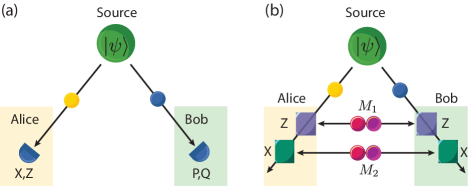
Figure 1: (a) CHSH setup: an entangled bipartite state $|\psi\rangle$ is divided, with one subsystem sent to Alice and the other to Bob. Alice measures $X,Z$, while Bob measures $P,Q$. (b) A proposed nonlocal measurement model. In this model, two meters M₁ and M₂ are used to measure $ZZ$ and $XX$.

To find the most effective EW, here we propose a variational entanglement witness (VEW) for the first time, which optimizes $\mathcal{W}$ to better detect entanglement for a given quantum state. The variational scheme proceeds as follows. First, the entanglement witness $\mathcal{W}$ is parameterized by $\bm{\upalpha}$, ie., $\mathcal{W}(\bm{\upalpha})$. The expectation value of this witness is then used as the cost function

$$\mathcal{C}(\bm{\upalpha})=\text{Tr}\big{[}\mathcal{W}(\bm{\upalpha})\rho\big{]}.$$ (5)

The optimization process is defined by

$$\bm{\upalpha}^{*} =\arg\min_{\{\bm{\upalpha}\}}\mathcal{C}(\bm{\upalpha})$$ (6)

$$\text{s.t.}\quad\mathcal{C}(\bm{\upalpha}^{*}) =0\quad\forall\text{ separable states }\rho_{\rm sep}.$$ (7)

The objective is to find $\bm{\upalpha}^{*}$ that minimizes the cost function, ideally achieving a negative value for entangled states.

In this work, we employ $S_{\rm CHSH}$ as the variational witness operator, thereby removing the requirement for prior knowledge of the quantum state and enabling direct measurement. The variational witness operator is defined by

$$\mathcal{W}(\bm{\upalpha})=-\sqrt{2}\big{(}\alpha_{1}ZZ+\alpha_{2}XX\big{)},$$ (8)

with the cost function is

$$\mathcal{C}(\bm{\upalpha})=-\sqrt{2}\big{(}\alpha_{1}\langle ZZ\rangle+\alpha_{2}\langle XX\rangle\big{)}.$$ (9)

The optimization process bases on gradient-free methods using the COBYLA optimizer. See detailed calculation in Appendix C. The results, illustrated in Fig. 2(b), effectively demonstrate the entanglement of the quantum state $|\psi\rangle$. Specifically, at $\theta=0,\pi/2,$ and $\pi$, the expectation value $\langle\mathcal{W}(\bm{\upalpha}^{*})\rangle$ is zero, indicating zero in the PPT criterion and concurrence. At other points, $\langle\mathcal{W}(\bm{\upalpha}^{*})\rangle$ is negative, signifying entanglement. This observation holds for all $\phi$ except when $\phi=\pi/2$, because at this specific point, the expectation value $\langle XX\rangle=0$ and thus $\mathcal{C}(\bm{\upalpha})$ becomes a constant. According to the constrain in Eq. (7), this $\mathcal{C}(\bm{\upalpha})$ must be vanished.

We emphasize that both the CHSH inequality and VEW require nonlocal measurements of the expectation values $\langle ZZ\rangle$ and $\langle XX\rangle$. We will now present a framework for nonlocal measurements of $\langle ZZ\rangle$ and $\langle XX\rangle$ to confirm the CHSH inequality and VEW.

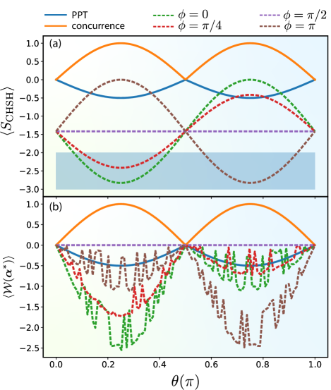
Figure 2: (a) Plot of $\langle S_{\rm CHSH}\rangle$ versus $\theta$ at different $\phi$ values. The CHSH inequality is violated in the aqua region where $|\langle S_{\rm CHSH}\rangle|>2$. Entanglement measures including the PPT criterion and concurrence are also shown for comparison. (b) Plot of the optimal entanglement witness $\langle\mathcal{W}(\bm{\upalpha}^{*})\rangle$.

II.2 Nonlocal measurement framework for measuring the CHSH inequality and VEW

To measure $X$ and $Z$ on the Alice’s side and $P$ and $Q$ on the Bob’s side, we need to measure the nonlocal products $Z\otimes Z$ and $X\otimes X$, or $ZZ$ and $XX$ for short. This is challenging because measuring noncommutative observables in a local state is impossible. To overcome this problem, we use entangled meters to couple to both Alice’s and Bob’s sides and readout the meters’ outcomes. The initial meters states are maximally entangled Bell states. Alice and Bob each couple their subsystem with the meters. After the interactions, they measure their meter in the $Z$ bases.

The nonlocal measurement model is shown in Fig. 1(b). To measure $\langle ZZ\rangle$ and $\langle XX\rangle$ simultaneously, we use two meters, $\rm M_{1}$ and $\rm M_{2}$. The meter states are given by Bell states as

$$|\xi\rangle_{1} =\dfrac{1}{\sqrt{2}}\Big{(}|\uparrow\uparrow\rangle+|\downarrow\downarrow\rangle\Big{)}$$ (10)

$$|\xi\rangle_{2} =\dfrac{1}{\sqrt{2}}\Big{(}|\circ\!\times\rangle+|\times\!\circ\rangle\Big{)},$$ (11)

where we used $\{|\uparrow\rangle,|\downarrow\rangle\}$ as the computational basis for M₁ and $\{|\circ\rangle,|\times\rangle\}$ for M₂, which are equivalent to $\{|0\rangle,|1\rangle\}$ in system S.

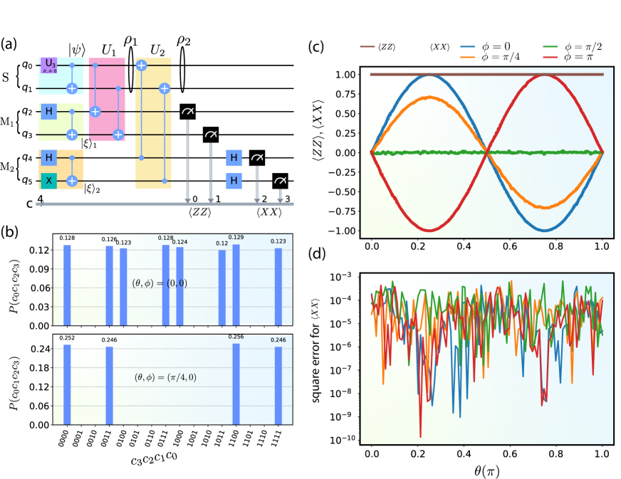
Figure 3: (a) Quantum circuit for nonlocal measurement: System S consists of two qubits, $q_{0}$ and $q_{1}$, meter M₁ consists of $q_{2}$ and $q_{3}$, and meter M₂ consists of $q_{4}$ and $q_{5}$. (b) Probability $P(c_{0}c_{1}c_{2}c_{3})$ plotted for two cases: $(\theta,\phi)=(0,0)$ and $(\pi/4,0)$. (c) Plot of $\langle ZZ\rangle$ and $\langle XX\rangle$ versus $\theta$ at different $\phi$ values. The dotted curves are theoretical predictions, and the solid curves are from simulations. (d) Corresponding square error between simulations and theory plotted for $\langle XX\rangle$ case.

To measure $\langle ZZ\rangle$, we apply the interaction $U_{1}$ between the system and M₁ which are two CNOT (CX) gates as shown in Fig. 3(a). The measurement observables are represented by Kraus operators as

$$M_{\mu}=\langle\mu|U_{1}|\xi\rangle_{1},\ \forall\mu\in\{\uparrow\uparrow,\uparrow\downarrow,\downarrow\uparrow,\downarrow\downarrow\},$$ (12)

which gives

$$M_{\uparrow\uparrow} =M_{\downarrow\downarrow}=\dfrac{1}{\sqrt{2}}\big{(}|00\rangle\langle 00|+|11\rangle\langle 11|\big{)},$$ (13)

$$M_{\uparrow\downarrow} =M_{\downarrow\uparrow}=0.$$ (14)

Refer to Appendix D for detailed calculations. From these measurements, we obtain the probabilities $P_{\mu}=\langle\psi|M_{\mu}^{\dagger}M_{\mu}|\psi\rangle$ as

$$P_{\uparrow\uparrow}=P_{\downarrow\downarrow}=\dfrac{1}{2};\ P_{\uparrow\downarrow}=P_{\downarrow\uparrow}=0.$$ (15)

Then, the expectation value $\langle ZZ\rangle$ yields

$$\langle ZZ\rangle=P_{\uparrow\uparrow}-P_{\uparrow\downarrow}-P_{\downarrow\uparrow}+P_{\downarrow\downarrow}=1.$$ (16)

Similarly, we measure $\langle XX\rangle$ using meter M₂, which interacts with the system through $U_{2}$, represented by two inverted CX gates as shown in Fig. 3(a). The measured operators are given by

$$N_{\circ\circ} =-N_{\times\times}=\dfrac{1}{2\sqrt{2}}\big{(}IX+XI\big{)},$$ (17)

$$-N_{\circ\times} =N_{\times\circ}=\dfrac{1}{2\sqrt{2}}\big{(}IX-XI\big{)},$$ (18)

and the corresponding probabilities are

$$P_{\circ\circ} =P_{\times\!\times}=\dfrac{1}{4}\big{(}1+\cos\phi\sin 2\theta\big{)},$$ (19)

$$P_{\circ\times} =P_{\times\circ}=\dfrac{1}{4}\big{(}1-\cos\phi\sin 2\theta\big{)}.$$ (20)

Finally, the expectation value $\langle XX\rangle$ is calculated as

$$\langle XX\rangle=P_{\circ\circ}-P_{\circ\times}-P_{\times\circ}+P_{\times\times}=\cos\phi\sin 2\theta.$$ (21)

Refer to detailed calculations in Append D. Consequently, both $\langle ZZ\rangle$ and $\langle XX\rangle$ can be measured through nonlocal measurements, thereby verifying the $S_{\text{CHSH}}$ inequality, and can also be used for optimizing the VEW.

II.3 Simulation on superconducting chip

We design a quantum circuit as shown in Fig. 3(a) for measuring $\langle ZZ\rangle$ and $\langle XX\rangle$. System S is $q_{0}q_{1}$, meter M₁ is given by $q_{2}q_{3}$, and meter M₂ is given by $q_{4}q_{5}$. The system state $|\psi\rangle$ is prepared by applying a quantum gate U₃ onto $q_{0}$ and a CX gate onto $q_{0}q_{1}$, where

$${\rm U}_{3}(\theta,\phi,\lambda)=\begin{pmatrix}\cos\frac{\theta}{2}&-e^{i\lambda}\sin\frac{\theta}{2}\\ e^{i\phi}\sin\frac{\theta}{2}&e^{i(\phi+\lambda)}\cos\frac{\theta}{2}\end{pmatrix},$$ (22)

where we used $2\theta$ in Eq. (22) to get $|\psi\rangle$. Similarly, to prepare $|\xi\rangle_{1}$, we apply a Hadamard gate onto $q_{2}$ followed by a CX gate $q_{2}q_{3}$, and to prepare $|\xi\rangle_{2}$, we apply a Hadamard gate onto $q_{4}$, X gate onto $q_{5}$, followed by a CX gate $q_{4}q_{5}$. The interaction $U_{1}$ consists of two CX gates, while $U_{2}$ consists of two inverted CX gates as shown in the figure. Measure $q_{2},q_{3}$ in the $Z$ basis gives the outcome for $\langle ZZ\rangle$. To get $\langle XX\rangle$, we apply Hadamard gates onto $q_{4}$ and $q_{5}$, and measure in the $Z$ basis.

For the numerical experiment, we execute the quantum circuit using Qiskit simulation. For each data point, we run 10000 shots and obtain the classical probability $P(c_{0}c_{1}c_{2}c_{3})$, which is the outcome of the two meters M₁ and M₂, where $c_{0}c_{1}$ are the classical outcomes of M₁ and $c_{2}c_{3}$ are the outcomes of M₂.

In Fig. 3(b), we show $P(c_{0}c_{1}c_{2}c_{3})$ for several cases of $(\theta,\phi)$, including $(\theta,\phi)=(0,0)$ and $(\theta,\phi)=(\pi/4,0)$. First, we emphasize the bases denotation in Tab. 1 below.

Table 1: Bases denotation that used in the meters.

	Bases
Meter	0	1
M1	$\uparrow$	$\downarrow$
M2	$\circ$	$\times$

For example, $c_{0}c_{1}c_{2}c_{3}=\text{`}0101\text{'}$ means $\text{`}\uparrow\downarrow\circ\times\text{'}$. With this rule, the probabilities give

$$P_{ij} =\sum_{\{k,l\}\in\{\circ,\times\}}P(ijkl),$$ (23)

$$P_{kl} =\sum_{\{i,j\}\in\{\uparrow,\downarrow\}}P(ijkl),$$ (24)

where $\{i,j\}\in\{\uparrow,\downarrow\}$ and $\{k,l\}\in\{\circ,\times\}$. Using these probabilities, we can calculate the nonlocal expectation values $\langle ZZ\rangle$ and $\langle XX\rangle$.

In Fig. 3(c), $\langle ZZ\rangle$ and $\langle XX\rangle$ are shown as functions of $\theta$ for different $\phi$ values. Simulation and theoretical results of these expectation values are compared and show good agreement. The corresponding square errors for $\langle XX\rangle$ are shown in Fig. 3(d) which are reasonable. These results show the effectiveness of nonlocal measurement in verifying the CHSH inequality and VEW.

II.4 Post-measurement quantum state

We derive the system state after these nonlocal measurements. The system (density) state after the first measurement gives [47]

$$\rho_{1}=\sum_{\mu}M_{\mu}|\psi\rangle\langle\psi|M_{\mu}^{\dagger}=|\psi\rangle\langle\psi|,$$ (25)

see Appendix E for detailed calculation. Next, we derive the system state after the second measurement. It gives

$$\rho_{2}=\sum_{\nu}N_{\nu}\rho_{1}N_{\nu}^{\dagger}=\dfrac{1}{2}\begin{pmatrix}0&0&0&0\\ 0&1&\cos\phi\sin 2\theta&0\\ 0&\cos\phi\sin 2\theta&1&0\\ 0&0&0&0\end{pmatrix}.$$ (26)

For example, Fig. 4(a) shows the tomography result of the final system state for $\theta=\phi=\pi/4$, which matches the theoretical calculation from Eq. (26).

Finally, we analyze the PPT criterion and concurrence of the final state to validate the protection of entanglement. For $\theta=k\pi/2$ or $\phi=\pi/2+k\pi$ for all $k\in\mathbb{N}$, the quantum state is $\rho_{2}={\rm diag}\big{(}0,1,1,0\big{)}/2$, where both the PPT criterion and concurrence are zero. This is depicted by the green dashed line in Fig. 4(b), ie., $\phi=\pi/2$. The polar plot of PPT criterion and concurrence against $\theta$ for different $\phi$ demonstrates that maximum entanglement occurs at $\theta=(2k+1)\pi/4$. These results indicate that entanglement is preserved under nonlocal measurement.

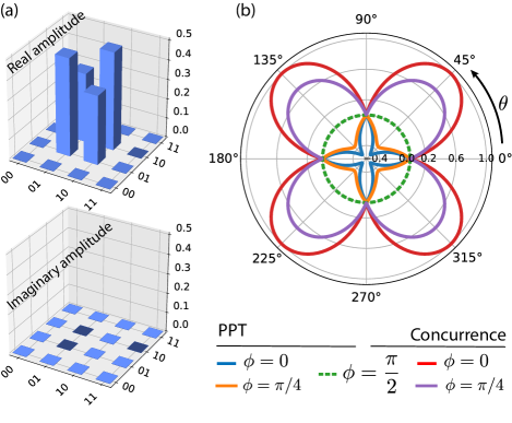
Figure 4: (a) Tomography of the final system state at $\theta=\phi=\pi/4$. (b) Polar plot of the PPT criterion and concurrence for the final state as functions of $\theta$ with different $\phi$ values.

II.5 Mixed state case

In this section, we examine $\langle S_{\rm CHSH}\rangle$ and its indication for the entanglement in mixed-state cases. We consider the Werner state as the system state

$$\rho=p|\Psi^{-}\rangle\langle\Psi^{-}|+\dfrac{1-p}{4}\bm{I},$$ (27)

where $0\leq p\leq 1$ and the Bell states (in the system bases) are defined by

$$|\Phi^{\pm}\rangle =\dfrac{1}{\sqrt{2}}\Bigl{(}|00\rangle\pm|11\rangle\Bigr{)},\text{and }$$ (28)

$$|\Psi^{\pm}\rangle =\dfrac{1}{\sqrt{2}}\Bigl{(}|01\rangle\pm|10\rangle\Bigr{)}.$$ (29)

Using the same meters M₁ and M₂ above, that means the same POVM as shown in Eqs. (D.7, D.8) and Eqs. (D.18, D.19). Then, we have

$$P_{\uparrow\uparrow} =P_{\downarrow\downarrow}={\rm tr}[\rho E_{\uparrow\uparrow}]=\dfrac{1-p}{4},$$ (30)

$$P_{\uparrow\downarrow} =P_{\downarrow\uparrow}={\rm tr}[\rho E_{\uparrow\downarrow}]=\dfrac{1+p}{4},$$ (31)

$$P_{\circ\circ} =P_{\times\times}={\rm tr}[\rho E_{\circ\circ}]=\dfrac{1-p}{4},$$ (32)

$$P_{\circ\times} =P_{\times\circ}={\rm tr}[\rho E_{\circ\times}]=\dfrac{1+p}{4}.$$ (33)

As a result, we have $\langle ZZ\rangle+\langle XX\rangle=-2p$, which implies $\langle S_{\rm CHSH}\rangle=2\sqrt{2}p$. The CHSH inequality (2) is violated when $1/\sqrt{2}<p\leq 1$. As previously stated, this violation region also exhibits entanglement.

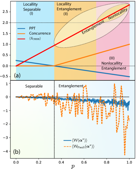
Figure 5: (a) Plot of $\langle S_{\rm CHSH}\rangle$, PPT criterion, and concurrence as functions of $p$. (b) Plot of the optimal entanglement witness $\langle\mathcal{W}(\bm{\upalpha}^{*})\rangle$, and $\langle\mathcal{W}_{\rm Pauli}(\bm{\upalpha}^{*})\rangle$.

To further explore the entanglement behavior, we again calculate the PPT criterion and concurrence, with results shown in Fig. 5(a). First, in region I (sky blue area), $0\leq p\leq 1/3$, the system state is local and there is no entanglement, ie., the PPT criterion is positive and the concurrence is zero. In region II (orange area), $1/3<p\leq 1/\sqrt{2}$, the system is local but exhibits entanglement. Finally, in region III (light pink area), $1/\sqrt{2}<p\leq 1$, the system state is nonlocal and entangled. This analysis demonstrates that while nonlocal behavior can indicate entanglement, the reverse is not necessarily true. To further clarify, we provide a Venn diagram indicating the relationship between nonlocality and entanglement.

To fully detect entanglement, we use the VEW $\mathcal{W}(\bm{\alpha})$ as defined in Eq. (8) and compare its performance with the standard Pauli case, $\mathcal{W}_{\rm Pauli}(\bm{\alpha})=\alpha_{1}XX+\alpha_{2}YY+\alpha_{3}ZZ$. The results in Fig. 5(b) show that the Pauli-based witness often fails to distinguish between entanglement and separability. In contrast, the $\mathcal{W}(\bm{\alpha})$ case successfully detects entanglement for $p\geq 1/3$, ie., $\mathcal{W}(\bm{\alpha}^{*})<0$, and identifies separable states for $p<1/3$, ie., $\mathcal{W}(\bm{\alpha}^{*})\approx 0$. However, the differentiation between entangled and separable states becomes ambiguous around the critical value of $p=1/3$, making it challenging to conclusively determine the state.

Next, we derive the post-measurement states, which are given through

$$\rho_{1}=\sum_{\mu}M_{\mu}\rho M_{\mu}^{\dagger}=\rho,$$ (34)

and

$$\rho_{2}=\sum_{\nu}N_{\nu}\rho_{1}N_{\nu}^{\dagger}=\begin{pmatrix}\frac{1+p}{4}&0&0&-\frac{p}{2}\\ 0&\frac{1-p}{4}&0&0\\ 0&0&\frac{1-p}{4}&0\\ -\frac{p}{2}&0&0&\frac{1+p}{4}\end{pmatrix}.$$ (35)

See detailed calculation in Appendix F. Finally, we observe that the entanglement in this state remains unchanged from the initial state $\rho$, indicating that entanglement persists under nonlocal measurement.

III Conclusion

We made significant progress in detecting and protecting quantum entanglement using nonlocality, variational entanglement witness (VEW), and nonlocal measurements. While traditional methods like violations of the CHSH inequality are effective, they do not cover all scenarios of entanglement detection. By introducing VEW, we addressed the limitations of these traditional methods, offered a more comprehensive approach to identifying entanglement. We also proposed a nonlocal measurement framework for measuring the CHSH operator and VEW.

Our findings emphasize the crucial role of nonlocal measurements in detecting and maintaining entanglement, which are essential for the functionality of quantum technologies. This work not only advances the understanding of quantum entanglement but also contributes to the practical development of more robust quantum computing, communication, and sensing systems.

Appendix A CHSH inequality

In this Appendix, we derive details of the CHSH inequality. We start from Eq. (1) in the main text as

$$S_{\rm CHSH}=(X+Z)\otimes P+(X-Z)\otimes Q.$$ (A.1)

Using $P=-(Z+X)/\sqrt{2},\ Q=(Z-X)/\sqrt{2}$, we have

$$S_{\rm CHSH} =-(X+Z)\otimes\dfrac{(Z+X)}{\sqrt{2}}+(X-Z)\otimes\dfrac{(Z-X)}{\sqrt{2}}$$

$$=-\sqrt{2}(XX+ZZ).$$ (A.2)

Now, the expectation value gives

$$\langle S_{\rm CHSH}\rangle =-\sqrt{2}\langle\psi|\big{(}XX+ZZ\big{)}|\psi\rangle$$

$$=-\sqrt{2}\big{(}\langle 00|\cos\theta+e^{-i\phi}\sin\theta\langle 11|\big{)}$$

$$\times\Big{[}(|00\rangle+|11\rangle)(\langle 00|+\langle 11|)-$$

$$\hskip 14.22636pt(|01\rangle-|10\rangle)(\langle 01|-\langle 10|)\Big{]}$$

$$\hskip 28.45274pt\times\big{(}\cos\theta|00\rangle+e^{i\phi}\sin\theta|11\rangle\big{)}$$

$$=-\sqrt{2}(\cos^{2}\theta+\sin^{2}\theta+\dfrac{1}{2}(2\cos\phi)\sin 2\theta)$$

$$=-\sqrt{2}(1+\cos\phi\sin 2\theta)$$ (A.3)

Appendix B Entanglement measures

We discuss various entanglement measures here, including the PPT criterion [15, 16] and concurrence [17] for bipartite systems. Let $\rho$ be a density matrix of an arbitrary mixed state of the two-qubit system AB. Its partial transpose (with respect to the B party) is defined as

$$\rho^{T_{B}}=(I\otimes T)[\rho].$$ (B.1)

If $\rho^{T_{B}}$ has a negative eigenvalue, $\rho$ is guaranteed to be entangled.

For concurrent, we first derive $\rho_{C}$ as

$$\rho_{C}=(Y\otimes Y)\rho^{*}(Y\otimes Y),$$ (B.2)

where $\rho^{*}$ is the complex conjugate of $\rho$. Let $\lambda_{1}\geq\lambda_{2}\geq\lambda_{3}\geq\lambda_{4}$ are eigenvalues of $\rho_{C}$, the concurrence is defined by

$$\mathcal{C}(\rho)=\max\big{\{}0,\lambda_{1}-\lambda_{2}-\lambda_{3}-\lambda_{4}\big{\}}.$$ (B.3)

The bipartite system is entangled if $\mathcal{C}(\rho)>0$ and the maximum of $\mathcal{C}(\rho)$ means the maximum of entanglement.

Appendix C Variation entanglement witness

In this section, we outline the optimization process for the variational entanglement witness. The cost function is defined as:

$$\mathcal{C}(\bm{\upalpha})=\text{Tr}\big{[}\mathcal{W}(\bm{\upalpha})\rho\big{]},$$ (C.1)

where $\mathcal{W}(\bm{\upalpha})$ is a Hermitian operator parameterized by $\bm{\upalpha}$, and $\rho$ is the quantum state of interest.

To minimize the cost function, we use the gradient-free COBYLA optimizer. This optimization yields the final parameters $\bm{\upalpha}^{*}$, which minimize the cost function $\mathcal{C}(\bm{\upalpha})$ and represent the optimal parameters for minimizing $\text{Tr}[\mathcal{W}(\bm{\upalpha})\rho]$.

For pure states, where $\mathcal{W}(\bm{\upalpha})=-\sqrt{2}(\alpha_{1}ZZ+\alpha_{2}XX)$ and $\rho=|\psi\rangle\langle\psi|$, we use the set of separable states $\{|00\rangle\langle 00|,|01\rangle\langle 01|,|10\rangle\langle 10|,|11\rangle\langle 11|\}$. The initial parameters are $\bm{\upalpha}=[4.0,0.0]$.

For mixed states, we use both the witness operator $\mathcal{W}(\bm{\upalpha})$ and a Pauli-based witness operator $\mathcal{W}_{\rm Pauli}(\bm{\upalpha})=\alpha_{1}XX+\alpha_{2}YY+\alpha_{3}ZZ$. The quantum state $\rho$ is the Werner state, as defined in Eq. (27). In addition to the previous separable states, we include $\rho(p=0)=\bm{I}/4$. The initial parameters for the Pauli-based case are chosen randomly.

Appendix D Nonlocal measurement

In this section, we derive detailed calculation of nonlocal measurement of $\langle ZZ\rangle$ and $\langle XX\rangle$.

D.1 Nonlocal measurement of $\langle ZZ\rangle$

The measurement of $\langle ZZ\rangle$ is given though meter M₁ initially prepare in $|\xi\rangle_{1}=\dfrac{1}{\sqrt{2}}\big{(}|\uparrow\uparrow\rangle+|\downarrow\downarrow\rangle\big{)}$. First, the interaction between the system and meter M₁ is give through $U_{1}$, which are CX gates as

$${\rm CX}_{q_{0}q_{2}}\ {\rm CX}_{q_{1}q_{3}} =\Big{(}|0\rangle\langle 0|_{q_{0}}\otimes I_{q_{2}}+|1\rangle\langle 1|_{q_{0}}\otimes X_{q_{2}}\Big{)}\Big{(}|0\rangle\langle 0|_{q_{1}}\otimes I_{q_{3}}+|1\rangle\langle 1|_{q_{1}}\otimes X_{q_{3}}\Big{)}$$

$$=\Big{(}|00\rangle\langle 00|_{q_{0}q_{1}}\otimes I_{q_{2}}I_{q_{3}}+|01\rangle\langle 01|_{q_{0}q_{1}}\otimes I_{q_{2}}X_{q_{3}}+|10\rangle\langle 10|_{q_{0}q_{1}}\otimes X_{q_{2}}I_{q_{3}}+|11\rangle\langle 11|_{q_{0}q_{1}}\otimes X_{q_{2}}X_{q_{3}}\Big{)},$$ (D.1)

where CX${}_{q_{i}q_{j}}$ is a CNOT gate with the control qubit is $q_{i}$ and the target qubit is $q_{j}$. The action of $U_{1}$ onto $|\xi\rangle_{1}$ gives

$$U_{1}|\xi\rangle_{1} =\Big{(}|00\rangle\langle 00|\otimes II+|01\rangle\langle 01|\otimes IX+|10\rangle\langle 10|\otimes XI+|11\rangle\langle 11|\otimes XX\Big{)}\otimes\dfrac{1}{\sqrt{2}}\big{(}|\uparrow\uparrow\rangle+|\downarrow\downarrow\rangle\big{)}\big{)}$$

$$=\dfrac{1}{\sqrt{2}}\Big{(}|00\rangle\langle 00|+|11\rangle\langle 11|\Big{)}\otimes\Big{(}|\uparrow\uparrow\rangle+|\downarrow\downarrow\rangle\Big{)}+\Big{(}|01\rangle\langle 01|+|10\rangle\langle 10|\Big{)}\otimes\Big{(}|\uparrow\downarrow\rangle+|\downarrow\uparrow\rangle\Big{)}.$$ (D.2)

The measure observables are given in Kraus operators as $M_{\mu}=\langle\mu|U_{1}|\xi\rangle_{1},\forall\mu\in\{\uparrow\uparrow,\uparrow\downarrow,\downarrow\uparrow,\downarrow\downarrow\}$, where

$$M_{\uparrow\uparrow} =\langle\uparrow\uparrow|U_{1}|\xi\rangle_{1}=\dfrac{1}{\sqrt{2}}\big{(}|00\rangle\langle 00|+|11\rangle\langle 11|\big{)},$$ (D.3)

$$M_{\uparrow\downarrow} =\langle\uparrow\downarrow|U_{1}|\xi\rangle_{1}=\dfrac{1}{\sqrt{2}}\big{(}|01\rangle\langle 01|+|10\rangle\langle 10|\big{)},$$ (D.4)

$$M_{\downarrow\uparrow} =\langle\downarrow\uparrow|U_{1}|\xi\rangle_{1}=\dfrac{1}{\sqrt{2}}\big{(}|01\rangle\langle 01|+|10\rangle\langle 10|\big{)},$$ (D.5)

$$M_{\downarrow\downarrow} =\langle\downarrow\downarrow|U_{1}|\xi\rangle_{1}=\dfrac{1}{\sqrt{2}}\big{(}|00\rangle\langle 00|+|11\rangle\langle 11|\big{)}.$$ (D.6)

We next calculate the positive operator-valued measure (POVM) $E_{\mu}=M_{\mu}^{\dagger}M_{\mu}$, which give

$$E_{\uparrow\uparrow}=E_{\downarrow\downarrow}=M_{\uparrow\uparrow}^{\dagger}M_{\uparrow\uparrow}=\dfrac{1}{2}\big{(}|00\rangle\langle 00|+|11\rangle\langle 11|\big{)},$$ (D.7)

$$E_{\uparrow\downarrow}=E_{\downarrow\uparrow}=M_{\uparrow\downarrow}^{\dagger}M_{\uparrow\downarrow}=\dfrac{1}{2}\big{(}|01\rangle\langle 01|+|10\rangle\langle 10|\big{)}.$$ (D.8)

And the probabilities yield

$$P_{\uparrow\uparrow} =\langle\psi|E_{\uparrow\uparrow}|\psi\rangle$$

$$=\big{(}\cos\theta\langle 00|+e^{-i\phi}\langle 11|\big{)}\dfrac{1}{2}\big{(}|00\rangle\langle 00|+|11\rangle\langle 11|\big{)}$$

$$\hskip 85.35826pt\times\big{(}\cos\theta|00\rangle+e^{i\phi}|11\rangle\big{)}$$

$$=\dfrac{1}{2},$$ (D.9)

and

$$P_{\uparrow\downarrow} =P_{\downarrow\uparrow}=\langle\psi|E_{\uparrow\downarrow}|\psi\rangle=0.$$ (D.10)

$$P_{\downarrow\downarrow} =\langle\psi|E_{\downarrow\downarrow}|\psi\rangle=\dfrac{1}{2}.$$ (D.11)

Finally, we obtain the expectation value

$$\langle ZZ\rangle=P_{\uparrow\uparrow}-P_{\uparrow\downarrow}-P_{\downarrow\uparrow}+P_{\downarrow\downarrow}=1,$$ (D.12)

as shown in Eq. (16) in the main text.

D.2 Nonlocal measurement of $\langle XX\rangle$

Similar, to measure $\langle XX\rangle$, we use meter M₂ with the initial state $|\xi\rangle_{2}=\dfrac{1}{\sqrt{2}}\big{(}|\circ\!\times\rangle+|\times\!\circ\rangle\big{)}$. The interaction $U_{2}$ is the invert CX gates

$$\bar{\rm CX}_{q_{0}q_{4}}\bar{\rm CX}_{q_{1}q_{5}} =\big{(}I_{q_{0}}\otimes|\circ\rangle\langle\circ|_{q_{4}}+X_{q_{0}}\otimes|\times\rangle\langle\times|_{q_{4}}\big{)}\big{(}I_{q_{1}}\otimes|\circ\rangle\langle\circ|_{q_{5}}+X_{q_{1}}\otimes|\times\rangle\langle\times|_{q_{5}}\big{)}$$

$$=II\otimes|\circ\!\circ\rangle\langle\circ\!\circ|+IX\otimes|\circ\!\times\rangle\langle\circ\!\times|+XI\otimes|\times\!\circ\rangle\langle\times\!\circ|+XX\otimes|\times\!\times\rangle\langle\times\!\times|,$$ (D.13)

where $q_{4}$ and $q_{5}$ are control qubits and $q_{0}$ and $q_{1}$ are target qubits. The action of $U_{2}$ on $|\xi\rangle_{2}$ gives

$$U_{2}|\xi\rangle_{2}=\dfrac{1}{\sqrt{2}}\Big{(}IX\otimes|\circ\!\times\rangle+XI\otimes|\times\!\circ\rangle\Big{)}.$$ (D.14)

After the interaction $U_{2}$, we apply the Hadamard gates ${\rm H}_{q_{4}}{\rm H}_{q_{5}}$ onto qubits $q_{4}$ and $q_{5}$ of the meter M₂

$${\rm H}_{q_{4}}{\rm H}_{q_{5}}U_{2}|\xi\rangle_{2} =\dfrac{1}{2\sqrt{2}}\Big{(}IX\otimes\big{[}|\circ\rangle+|\times\rangle\big{)}\big{(}|\circ\rangle-|\times\rangle\big{)}+XI\otimes\big{(}|\circ\rangle-|\times\rangle\big{)}\big{(}|\circ\rangle+|\times\rangle\big{)}\Big{]}$$

$$=\dfrac{1}{2\sqrt{2}}\Big{[}\big{(}IX+XI\big{)}\otimes\big{(}|\circ\!\circ\rangle-|\times\!\times\rangle\big{)}+\big{(}IX-XI\big{)}\otimes\big{(}-|\circ\!\times\rangle+|\times\!\circ\rangle\big{)}\Big{]}$$ (D.15)

where we used ${\rm H}|\circ\rangle=(|\circ\rangle+|\times\rangle)/\sqrt{2}$ and ${\rm H}|\times\rangle=(|\circ\rangle-|\times\rangle)/\sqrt{2}$. We next calculate the Kraus operators $N_{\nu}=\langle\nu|{\rm H}_{q_{4}}{\rm H}_{q_{5}}U_{2}|\xi\rangle_{2}$, where $\nu\in\{\circ\circ,\circ\times,\times\circ,\times\times\}$. We have

$$N_{\circ\circ} =-N_{\times\times}=\dfrac{1}{2\sqrt{2}}\big{(}IX+XI\big{)},$$ (D.16)

$$-N_{\circ\times} =N_{\times\circ}=\dfrac{1}{2\sqrt{2}}\big{(}IX-XI\big{)},$$ (D.17)

and the corresponding POVM yields

$$E_{\circ\circ} =E_{\times\times}=\dfrac{1}{4}\big{(}II+XX\big{)},$$ (D.18)

$$E_{\circ\times} =E_{\times\circ}=\dfrac{1}{4}\big{(}II-XX\big{)},$$ (D.19)

which satisfies $\sum_{\nu}E_{\nu}=II$. The probabilities yield

$$P_{\circ\circ} =P_{\times\!\times}=\langle\psi|E_{\circ\circ}|\psi\rangle=\dfrac{1}{4}\big{(}1+\cos\phi\sin 2\theta\big{)},$$ (D.20)

$$P_{\circ\times} =P_{\times\circ}=\langle\psi|E_{\circ\times}|\psi\rangle=\dfrac{1}{4}\big{(}1-\cos\phi\sin 2\theta\big{)}.$$ (D.21)

Finally, we get the expectation value $\langle XX\rangle$

$$\langle XX\rangle=P_{\circ\circ}-P_{\circ\times}-P_{\times\circ}+P_{\times\!\times}=\cos\phi\sin 2\theta,$$ (D.22)

as shown in Eq. (21) in the main text.

Appendix E Post-measurement state

In this section, we derive the final system state after measuring M₁ and M₂. The system state after the first measurement gives $\rho_{1}=\sum_{\mu}M_{\mu}|\psi\rangle\langle\psi|M_{\mu}^{\dagger}$. We first derive

$$M_{\uparrow\uparrow}|\psi\rangle =\dfrac{1}{\sqrt{2}}\big{(}|00\rangle\langle 00|+|11\rangle\langle 11|\big{)}\big{(}\cos\theta|00\rangle+e^{i\phi}\sin\theta|11\rangle\big{)}$$

$$=\dfrac{1}{\sqrt{2}}|\psi\rangle,$$ (E.1)

and thus $M_{\uparrow\uparrow}|\psi\rangle\langle\psi|M^{\dagger}_{\uparrow\uparrow}=|\psi\rangle/2$. Similarly, we have $M_{\downarrow\downarrow}|\psi\rangle\langle\psi|M^{\dagger}_{\downarrow\downarrow}=|\psi\rangle/2$, and $M_{\uparrow\downarrow}|\psi\rangle\langle\psi|M^{\dagger}_{\uparrow\downarrow}=M_{\downarrow\uparrow}|\psi\rangle\langle\psi|M^{\dagger}_{\downarrow\uparrow}=0.$ Finally, we get

$$\rho_{1}=\sum_{\mu}M_{\mu}|\psi\rangle\langle\psi|M_{\mu}^{\dagger}=|\psi\rangle\langle\psi|,$$ (E.2)

Next, we derive the system state after the second measurement. It gives $\rho_{2}=\sum_{\nu}N_{\nu}\rho_{1}N_{\nu}^{\dagger}$. We first derive

$$N_{\circ\circ}|\psi\rangle =\dfrac{1}{2\sqrt{2}}\big{(}IX+XI\big{)}\big{(}\cos\theta|00\rangle+e^{i\phi}\sin\theta|11\rangle\big{)}$$

$$=\dfrac{1}{2\sqrt{2}}\big{(}\cos\theta+e^{i\phi}\sin\theta\big{)}\big{(}|01\rangle+|10\rangle\big{)},$$ (E.3)

and thus

$$\rho_{2}=\sum_{\nu}N_{\nu}\rho_{1}N_{\nu}^{\dagger}=\dfrac{1}{2}\begin{pmatrix}0&0&0&0\\ 0&1&\cos\phi\sin 2\theta&0\\ 0&\cos\phi\sin 2\theta&1&0\\ 0&0&0&0\end{pmatrix}.$$ (E.4)

Appendix F Mixed state case

In this section, we provide detailed calculations for mixed-state cases. We need to derive Eqs.(30-33). We first recast the quantum state in matrix form as

$$\rho=\begin{pmatrix}\frac{1-p}{4}&0&0&0\\ 0&\frac{1+p}{4}&-\frac{p}{2}&0\\ 0&-\frac{p}{2}&\frac{1+p}{4}&0\\ 0&0&0&\frac{1-p}{4}\end{pmatrix}.$$ (F.1)

The probabilities give

$$P_{\uparrow\uparrow} ={\rm Tr}\big{[}E_{\uparrow\uparrow}\rho\big{]}$$

$$=\dfrac{1}{2}{\rm Tr}\big{[}\big{(}|00\rangle\langle 00|+|11\rangle\langle 11\big{)}\rho\big{]}$$

$$=\dfrac{1}{2}\big{[}\langle 00|\rho|00\rangle+\langle 11|\rho|11\rangle\big{]}$$

$$=\dfrac{1-p}{4}.$$ (F.2)

Similarly, we have $P_{\downarrow\downarrow}=\dfrac{1-p}{4}$, and

$$P_{\uparrow\downarrow}=P_{\downarrow\uparrow} =\dfrac{1}{2}(\langle 01|\rho|01\rangle+\langle 10|\rho|10\rangle)$$

$$=\dfrac{1+p}{4}.$$ (F.3)

Finally, the expectation value for the measurement of $\langle ZZ\rangle$ gives

$$\langle ZZ\rangle =P_{\uparrow\uparrow}-P_{\uparrow\downarrow}-P_{\downarrow\uparrow}+P_{\downarrow\downarrow}$$

$$=\dfrac{1-p}{4}-\dfrac{1+p}{4}-\dfrac{1+p}{4}+\dfrac{1-p}{4}$$

$$=-p.$$ (F.4)

We can also take the expectation value for the measurement of $\langle$XX$\rangle$. First, we calculate the probabilities

$$P_{\circ\circ}=P_{\times\times} ={\rm Tr}\big{[}E_{\circ\circ}\rho\big{]}$$

$$=\dfrac{1}{4}{\rm Tr}\big{[}(II+XX)\rho\big{]}$$

$$=\dfrac{1-p}{4},$$ (F.5)

$$P_{\circ\times}=P_{\times\circ} ={\rm Tr}\big{[}E_{\circ\times}\rho\big{]}$$

$$=\dfrac{1}{4}{\rm Tr}\big{[}(II+XX)\rho\big{]}$$

$$=\dfrac{1+p}{4}$$ (F.6)

Then, the expectation value

$$\langle XX\rangle=-p.$$ (F.7)

The post-measurement states are given through $\rho_{1}=\sum_{\mu}M_{\mu}\rho M_{\mu}^{\dagger}$ and $\rho_{2}=\sum_{\nu}N_{\nu}\rho_{1}N_{\nu}^{\dagger}$ after measuring of M₁ and M₂, respectively. We first derive $M_{\mu}\rho M_{\mu}^{\dagger}$ for $\mu=\{\uparrow\uparrow,\uparrow\downarrow,\downarrow\uparrow,\downarrow\downarrow\}$, where

$$M_{\uparrow\uparrow}\rho M_{\uparrow\uparrow}^{\dagger}=\dfrac{1}{2}\begin{pmatrix}\frac{1-p}{4}&0&0&0\\ 0&0&0&0\\ 0&0&0&0\\ 0&0&0&\frac{1-p}{4}\end{pmatrix},$$ (F.8)

and similar for $M_{\downarrow\downarrow}\rho M_{\downarrow\downarrow}^{\dagger}$, and

$$M_{\uparrow\downarrow}\rho M_{\uparrow\downarrow}^{\dagger}=\dfrac{1}{2}\begin{pmatrix}0&0&0&0\\ 0&\frac{1+p}{4}&-\frac{p}{2}&0\\ 0&-\frac{p}{2}&\frac{1+p}{4}&0\\ 0&0&0&0\end{pmatrix},$$ (F.9)

and similar for $M_{\downarrow\uparrow}\rho M_{\downarrow\uparrow}^{\dagger}$. Finally, we have

$$\rho_{1}=\sum_{\mu}M_{\mu}\rho M_{\mu}^{\dagger}=\rho.$$ (F.10)

Similar for $\rho_{2}$, we obtain

$$\rho_{2}=\sum_{\nu}N_{\nu}\rho_{1}N_{\nu}^{\dagger}=\begin{pmatrix}\frac{1+p}{4}&0&0&-\frac{p}{2}\\ 0&\frac{1-p}{4}&0&0\\ 0&0&\frac{1-p}{4}&0\\ -\frac{p}{2}&0&0&\frac{1+p}{4}\end{pmatrix}.$$ (F.11)

References

- Horodecki et al. [2009] R. Horodecki, P. Horodecki, M. Horodecki, and K. Horodecki, Quantum entanglement, Rev. Mod. Phys. 81, 865 (2009).
- Duarte [2022] F. J. Duarte, Fundamentals of Quantum Entanglement (Second Edition), 2053-2563 (IOP Publishing, 2022).
- Yu [2021] Y. Yu, Advancements in applications of quantum entanglement, Journal of Physics: Conference Series 2012, 012113 (2021).
- Yin et al. [2020] J. Yin, Y.-H. Li, S.-K. Liao, M. Yang, Y. Cao, L. Zhang, J.-G. Ren, W.-Q. Cai, W.-Y. Liu, S.-L. Li, R. Shu, Y.-M. Huang, L. Deng, L. Li, Q. Zhang, N.-L. Liu, Y.-A. Chen, C.-Y. Lu, X.-B. Wang, F. Xu, J.-Y. Wang, C.-Z. Peng, A. K. Ekert, and J.-W. Pan, Entanglement-based secure quantum cryptography over 1,120 kilometres, Nature 582, 501 (2020).
- Basset et al. [2021] F. B. Basset, M. Valeri, E. Roccia, V. Muredda, D. Poderini, J. Neuwirth, N. Spagnolo, M. B. Rota, G. Carvacho, F. Sciarrino, and R. Trotta, Quantum key distribution with entangled photons generated on demand by a quantum dot, Science Advances 7, eabe6379 (2021), https://www.science.org/doi/pdf/10.1126/sciadv.abe6379 .
- Zou [2021] N. Zou, Quantum entanglement and its application in quantum communication, Journal of Physics: Conference Series 1827, 012120 (2021).
- Wengerowsky et al. [2018] S. Wengerowsky, S. K. Joshi, F. Steinlechner, H. Hübel, and R. Ursin, An entanglement-based wavelength-multiplexed quantum communication network, Nature 564, 225 (2018).
- Guccione et al. [2020] G. Guccione, T. Darras, H. L. Jeannic, V. B. Verma, S. W. Nam, A. Cavaillès, and J. Laurat, Connecting heterogeneous quantum networks by hybrid entanglement swapping, Science Advances 6, eaba4508 (2020), https://www.science.org/doi/pdf/10.1126/sciadv.aba4508 .
- Huang et al. [2024] J. Huang, M. Zhuang, and C. Lee, Entanglement-enhanced quantum metrology: From standard quantum limit to Heisenberg limit, Applied Physics Reviews 11, 031302 (2024), https://pubs.aip.org/aip/apr/article-pdf/doi/10.1063/5.0204102/20027645/031302_1_5.0204102.pdf .
- Augusiak et al. [2016] R. Augusiak, J. Kołodyński, A. Streltsov, M. N. Bera, A. Acín, and M. Lewenstein, Asymptotic role of entanglement in quantum metrology, Phys. Rev. A 94, 012339 (2016).
- Gühne and Tóth [2009] O. Gühne and G. Tóth, Entanglement detection, Physics Reports 474, 1 (2009).
- Gurvits [2004] L. Gurvits, Classical complexity and quantum entanglement, Journal of Computer and System Sciences 69, 448 (2004), special Issue on STOC 2003.
- James et al. [2001] D. F. V. James, P. G. Kwiat, W. J. Munro, and A. G. White, Measurement of qubits, Phys. Rev. A 64, 052312 (2001).
- Thew et al. [2002] R. T. Thew, K. Nemoto, A. G. White, and W. J. Munro, Qudit quantum-state tomography, Phys. Rev. A 66, 012303 (2002).
- Peres [1996] A. Peres, Separability criterion for density matrices, Phys. Rev. Lett. 77, 1413 (1996).
- Horodecki et al. [1996] M. Horodecki, P. Horodecki, and R. Horodecki, Separability of mixed states: necessary and sufficient conditions, Physics Letters A 223, 1 (1996).
- Hill and Wootters [1997] S. A. Hill and W. K. Wootters, Entanglement of a pair of quantum bits, Phys. Rev. Lett. 78, 5022 (1997).
- Elben et al. [2020] A. Elben, R. Kueng, H.-Y. R. Huang, R. van Bijnen, C. Kokail, M. Dalmonte, P. Calabrese, B. Kraus, J. Preskill, P. Zoller, and B. Vermersch, Mixed-state entanglement from local randomized measurements, Phys. Rev. Lett. 125, 200501 (2020).
- Bourennane et al. [2004] M. Bourennane, M. Eibl, C. Kurtsiefer, S. Gaertner, H. Weinfurter, O. Gühne, P. Hyllus, D. Bruß, M. Lewenstein, and A. Sanpera, Experimental detection of multipartite entanglement using witness operators, Phys. Rev. Lett. 92, 087902 (2004).
- Trávníček et al. [2024] V. c. v. Trávníček, J. Roik, K. Bartkiewicz, A. Černoch, P. Horodecki, and K. Lemr, Sensitivity versus selectivity in entanglement detection via collective witnesses, Phys. Rev. Res. 6, 033056 (2024).
- Bae et al. [2020] J. Bae, D. Chruściński, and B. C. Hiesmayr, Mirrored entanglement witnesses, npj Quantum Information 6, 15 (2020).
- Siudzińska and Chruściński [2021] K. Siudzińska and D. Chruściński, Entanglement witnesses from mutually unbiased measurements, Scientific Reports 11, 22988 (2021).
- Roik et al. [2021] J. Roik, K. Bartkiewicz, A. Černoch, and K. Lemr, Accuracy of entanglement detection via artificial neural networks and human-designed entanglement witnesses, Phys. Rev. Appl. 15, 054006 (2021).
- Jiráková et al. [2024] K. Jiráková, A. Černoch, A. Barasiński, and K. Lemr, Enhancing collective entanglement witnesses through correlation with state purity, Scientific Reports 14, 16374 (2024).
- Bell [1964] J. S. Bell, On the einstein podolsky rosen paradox, Physics Physique Fizika 1, 195 (1964).
- Clauser and Shimony [1978] J. F. Clauser and A. Shimony, Bell’s theorem. experimental tests and implications, Reports on Progress in Physics 41, 1881 (1978).
- Clauser et al. [1969] J. F. Clauser, M. A. Horne, A. Shimony, and R. A. Holt, Proposed experiment to test local hidden-variable theories, Phys. Rev. Lett. 23, 880 (1969).
- Bartkiewicz et al. [2013] K. Bartkiewicz, B. Horst, K. Lemr, and A. Miranowicz, Entanglement estimation from bell inequality violation, Phys. Rev. A 88, 052105 (2013).
- Dong et al. [2023] D.-D. Dong, X.-K. Song, X.-G. Fan, L. Ye, and D. Wang, Complementary relations of entanglement, coherence, steering, and bell nonlocality inequality violation in three-qubit states, Phys. Rev. A 107, 052403 (2023).
- Li et al. [2020] M. Li, H. Qin, C. Zhang, S. Shen, S.-M. Fei, and H. Fan, Characterizing multipartite entanglement by violation of chsh inequalities, Quantum Information Processing 19, 142 (2020).
- Cortés-Vega et al. [2023] J. Cortés-Vega, J. F. Barra, L. Pereira, and A. Delgado, Detecting entanglement of unknown states by violating the clauser–horne–shimony–holt inequality, Quantum Information Processing 22, 203 (2023).
- Werner [1989] R. F. Werner, Quantum states with einstein-podolsky-rosen correlations admitting a hidden-variable model, Phys. Rev. A 40, 4277 (1989).
- Ureña et al. [2024] J. Ureña, A. Sojo, J. Bermejo-Vega, and D. Manzano, Entanglement detection with classical deep neural networks, Scientific Reports 14, 18109 (2024).
- Asif et al. [2023] N. Asif, U. Khalid, A. Khan, T. Q. Duong, and H. Shin, Entanglement detection with artificial neural networks, Scientific Reports 13, 1562 (2023).
- Koutný et al. [2023] D. Koutný, L. Ginés, M. Moczała-Dusanowska, S. Höfling, C. Schneider, A. Predojević, and M. Ježek, Deep learning of quantum entanglement from incomplete measurements, Science Advances 9, eadd7131 (2023), https://www.science.org/doi/pdf/10.1126/sciadv.add7131 .
- Qu et al. [2023] Y.-D. Qu, R.-Q. Zhang, S.-Q. Shen, J. Yu, and M. Li, Entanglement detection with complex-valued neural networks, International Journal of Theoretical Physics 62, 206 (2023).
- Luo et al. [2023] Y.-J. Luo, J.-M. Liu, and C. Zhang, Detecting genuine multipartite entanglement via machine learning, Phys. Rev. A 108, 052424 (2023).
- Roik et al. [2022] J. Roik, K. Bartkiewicz, A. Černoch, and K. Lemr, Entanglement quantification from collective measurements processed by machine learning, Physics Letters A 446, 128270 (2022).
- Greenwood et al. [2023] A. C. Greenwood, L. T. Wu, E. Y. Zhu, B. T. Kirby, and L. Qian, Machine-learning-derived entanglement witnesses, Phys. Rev. Appl. 19, 034058 (2023).
- Kookani et al. [2024] A. Kookani, Y. Mafi, P. Kazemikhah, H. Aghababa, K. Fouladi, and M. Barati, Xpookynet: advancement in quantum system analysis through convolutional neural networks for detection of entanglement, Quantum Machine Intelligence 6, 50 (2024).
- Hensen et al. [2015] B. Hensen, H. Bernien, A. E. Dréau, A. Reiserer, N. Kalb, M. S. Blok, J. Ruitenberg, R. F. L. Vermeulen, R. N. Schouten, C. Abellán, W. Amaya, V. Pruneri, M. W. Mitchell, M. Markham, D. J. Twitchen, D. Elkouss, S. Wehner, T. H. Taminiau, and R. Hanson, Loophole-free bell inequality violation using electron spins separated by 1.3 kilometres, Nature 526, 682 (2015).
- Cirel’son [1980] B. S. Cirel’son, Quantum generalizations of bell’s inequality, Letters in Mathematical Physics 4, 93 (1980).
- Chruściński and Sarbicki [2014] D. Chruściński and G. Sarbicki, Entanglement witnesses: construction, analysis and classification, Journal of Physics A: Mathematical and Theoretical 47, 483001 (2014).
- Simon [2000] R. Simon, Peres-horodecki separability criterion for continuous variable systems, Phys. Rev. Lett. 84, 2726 (2000).
- Tóth [2005] G. Tóth, Entanglement witnesses in spin models, Phys. Rev. A 71, 010301 (2005).
- Dowling et al. [2004] M. R. Dowling, A. C. Doherty, and S. D. Bartlett, Energy as an entanglement witness for quantum many-body systems, Phys. Rev. A 70, 062113 (2004).
- Ho and Imoto [2017] L. B. Ho and N. Imoto, Generalized modular-value-based scheme and its generalized modular value, Phys. Rev. A 95, 032135 (2017).