Implicit Reasoning in Deep Time Series Forecasting

Abstract

Recently, time series foundation models have shown promising zero-shot forecasting performance on time series from a wide range of domains. However, it remains unclear whether their success stems from a true understanding of temporal dynamics or simply from memorizing the training data. While implicit reasoning in language models has been studied, similar evaluations for time series models have been largely unexplored. This work takes an initial step toward assessing the reasoning abilities of deep time series forecasting models. We find that certain linear, MLP-based, and patch-based Transformer models generalize effectively in systematically orchestrated out-of-distribution scenarios, suggesting underexplored reasoning capabilities beyond simple pattern memorization.

Keywords Forecasting, Time Series Foundation Models, Implicit Reasoning, Memorization

1 Introduction

Foundation models have demonstrated an exceptional ability to generalize to previously unseen data in zero-shot prediction tasks. Inspired by the success of such models in Natural Language Processing, recent work has adapted Transformers to build time series foundation models (TSFM). Zero-shot inference is particularly important for time series models, which must handle complex patterns, seasonal variations, and emerging trends where little to no reference data may be available.

Foundation models are trained on large, diverse datasets, raising a critical question for time series forecasting: do these models generalize well because they learn underlying concepts of temporal dynamics, or do they simply memorize specific patterns seen during training? If those models rely on memorization, particularly in the form of time series pattern matching, it could lead to redundancy in the stored knowledge, parameter inefficiency, and possibly limit their ability to generalize well to out-of-distribution (OOD) data. Ideally, a TSFM should be capable of implicit reasoning, allowing it not to depend solely on memorization but to infer latent temporal dynamics. Such models would be able to generalize from fewer data points, offering enhanced parameter efficiency and robustness.

While extensive research has been conducted to evaluate memorization and implicit reasoning in language models, similar evaluations for time series models have been largely unexplored. In this work, we take an initial step toward evaluating the implicit reasoning capabilities of time series models in forecasting tasks. Our findings highlight the potential of linear, MLP-based, and patch-based Transformer models to perform well in carefully orchestrated OOD scenarios, suggesting that these models may have untapped capabilities in reasoning beyond mere memorization.

2 Related work

Implicit Reasoning in LLMs.

Prior research has explored implicit reasoning in language models [2, 1, 27, 22, 29]. Implicit reasoning is often assessed through tasks that require models to apply knowledge learned during training to new test instances. One common form is composition, where models must chain multiple facts to answer a question [22, 29, 27]. Other forms of implicit reasoning explored include comparison and inverse search [2, 1]. Comparison involves models making judgments about unseen or altered data, such as comparing attributes of entities observed during training. Inverse search tests the ability to retrieve information in the reverse order of the training task. For instance, identifying an entity based on its attributes when the model was trained for the reverse task. More information on related work is provided in Appendix A.1. No prior research has conducted controlled experiments in time series forecasting to evaluate implicit reasoning on OOD data. Our study addresses this gap by introducing a novel framework that aligns LLM research with time series models, offering insights into optimal architectures for future TSFM development.

Time Series Foundation Models.

Several foundation models, including Chronos [3], LagLlama [17], Moirai [24], MOMENT [10], TimesFM [7], and TimeGPT [9], have been developed for time series forecasting. Some studies have also examined the impact of learning with synthetic data [3, 7]. MOMENT analyzed embeddings from synthetic sinusoids to isolate components like trends, while Chronos showed strong performance in forecasting composite series but struggled with exponential trends. These works demonstrate that TSFMs can learn distinct time series functions, though it remains unclear if their success is due to large-scale training or inherent reasoning abilities.

3 Methods

3.1 Implicit Reasoning Tasks

Our goal is to evaluate the ability of time series models to perform implicit reasoning or knowledge manipulation on OOD time series, using several experiments inspired by language model literature [2, 1, 22, 27, 29]. We carefully design experiments to test 3 forms of implicit reasoning: composition, comparison, and inverse search. We follow the notation from [22, 29], where ‘facts’ are formatted as (subject, relation, object). For continuous data, we adapt this to (input, function, output), with $f(x)=\widecheck{x}$ defining the relationship between the function $f$, input $x$, and output $\widecheck{x}$.

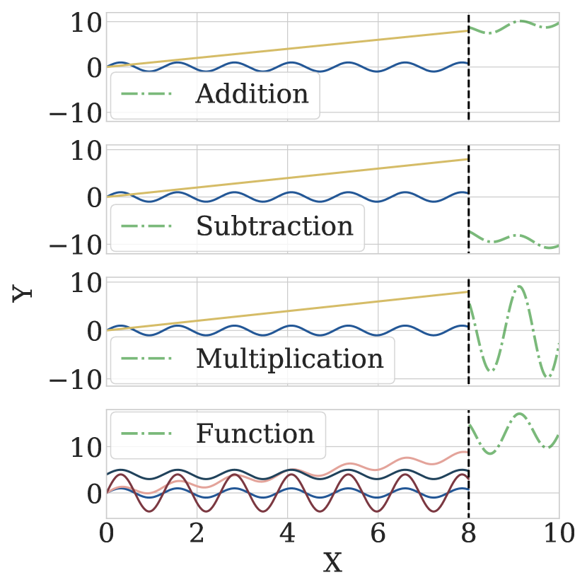
(a) Composition

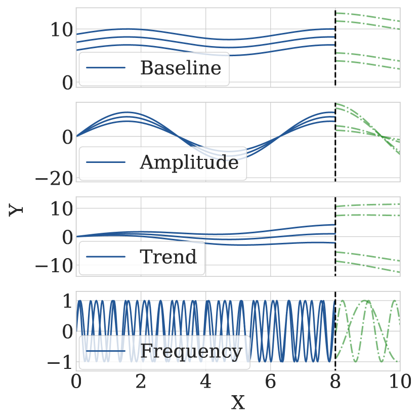
(b) Comparison

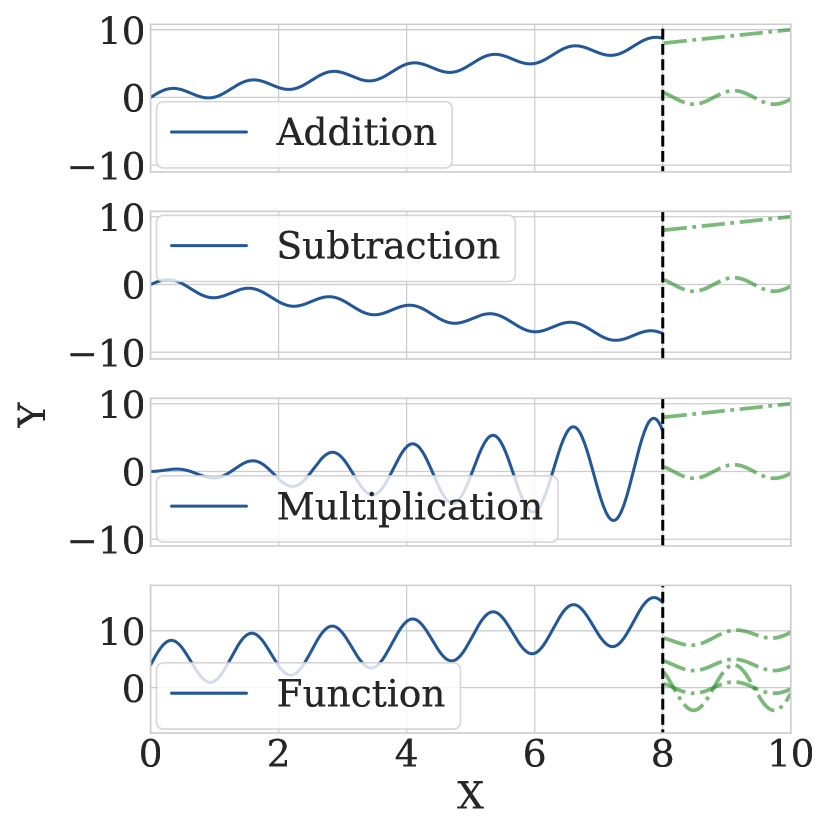
(c) Inverse Search

Figure 1: Implicit reasoning tasks for time series include composition (a), comparison (b), and inverse search (c). In composition, models predict new composite series seen only at inference. In comparison, they forecast series from unseen function values. In inverse search, models predict decomposed component series. The black dashed line in the figure indicates in-distribution time series observed during training (left) and out-of-distribution data observed during inference (right).

Composition.

We assess whether models can compose time series by applying knowledge manipulations similar to mathematical operations of addition, subtraction, and multiplication as illustrated in Fig. 1(a). We first define $\mathcal{F}$ as a set of basis functions. Given a set of input functions, $f_{1}$, the model must infer a set of composition functions $f_{2}$ to accurately forecast the OOD target signal, $y$. We define a composition rule based on prior work [22]:

$$f_{1},f_{2}\in\mathcal{F},\,\forall x\in\mathbb{R},(x,f_{1},\widecheck{x})\land(\widecheck{x},f_{2},y)\Rightarrow f_{2}(f_{1}(x))=y$$ (1)

For example, in addition composition tasks, $f_{2}=\sum_{i}f_{i}(x_{i})$ for all $f_{i}\in f_{1}$, where $f_{1}=\{\sin(x),mx\}$, encompassing trend and seasonality series. Models are trained exclusively on the individual component series, and the compositions of series are withheld for final evaluations. We train models on 30 trend and seasonality series ($n=60$) and evaluate them on all compositions of these series ($n=900$). In addition to the aforementioned composition tasks, we evaluate model performance on compositions involving sinusoidal signals with varying trends, frequencies, amplitudes, and baselines.

Comparison.

Comparison latent reasoning refers to a model’s ability to make comparative judgments on unseen or altered data. Our comparison task involves evaluating whether models can forecast series with component values that are greater or smaller than those in series used to train the model. Given a set of input functions, $f_{1}$, the model must infer a set of functions $f_{2}$ that scale $f_{1}$ to accurately forecast the OOD target signal, $y$. We define comparison rules based on [22]:

$$f_{1},f_{2}\in\mathcal{F},\,\forall x\in\mathbb{R},(x,f_{1},\widecheck{x})\land(\widecheck{x},f_{2},y)\land f_{1}(x)<y\Rightarrow f_{1}(x)<f_{2}(f_{1}(x))$$ (2)

$$f_{1},f_{2}\in\mathcal{F},\,\forall x\in\mathbb{R},(x,f_{1},\widecheck{x})\land(\widecheck{x},f_{2},y)\land f_{1}(x)>y\Rightarrow f_{1}(x)>f_{2}(f_{1}(x))$$ (3)

We train models on sinusoidal signals with varying trends, frequencies, amplitudes, and baselines ($n=1200$) and evaluate them on a subset of series with smaller or larger parameter values not seen during training ($n=120$).

Inverse search.

We evaluate whether models can ‘disentangle’ information through the inverse search task, which requires that models trained on composite signals are able to decompose time series into individual components during inference. Given a set of composition functions $f_{2}$, the model must infer a set of decomposed functions $f_{1}$ to accurately forecast each of the OOD target signals $y$. We define the inverse search rule as follows:

$$f_{1},f_{2}\in\mathcal{F},\,\forall x\in\mathbb{R},(x,f_{1},y)\land(y,f_{2},\widecheck{x})\Rightarrow f_{2}(f_{1}(x))=\widecheck{x}\land\forall f_{i}\in f_{1},\;f_{i}(x_{i})=y_{i}$$ (4)

We train models on composite addition of trend and seasonality series ($n=900$). We then evaluate the models on all decomposed trend and seasonality components series ($n=60$).

3.2 Data

We use the functions in Table 1, with parameter values detailed in Appendix A.3 to generate synthetic data. Both ID and OOD data use $x\in[0,1]$ with 1200 samples. Models are trained on the first 1000 ID samples and evaluated on the last 200 OOD samples, testing their implicit reasoning capabilities.

Table 1: Synthetic dataset functions and parameters for implicit reasoning tasks.

Task	Set	Function	Parameters
Composition	ID	$f_{1}(x)=\{\sin(B2\pi x),Mx\}$	$B,M$
(Add., Mult.)	OOD	$f_{2}(x)=\sin(B2\pi x)\!+\!Mx$
Composition	ID	$f_{1}(x)=\{\sin(B2\pi x),Mx\}$	$B,M$
(Sub.)	OOD	$f_{2}(x)=\sin(B2\pi x)\!-\!Mx$
Composition	ID	$f_{1}(x)=\{A\sin(2\pi x),\sin(B2\pi x),$	$A,B,C,M$
(Function)		$\sin(2\pi x)\!+\!C,\sin(2\pi x)\!+\!Mx\}$
	OOD	$f_{2}(x)=A\sin(B2\pi x)\!+\!C\!+\!Mx$
Comparison	ID	$f_{1}(x)=A\sin(B2\pi x)\!+\!D\!+\!Mx$	$A,B,C,M$
	OOD	$f_{2}(x)=a\sin(b2\pi x)\!+\!c\!+\!mx$	$a\!<\!A\!\lor\!a\!>\!A$, $b\!<\!B\!\lor\!b\!>\!B$
			$c\!<\!C\!\lor\!c\!>\!C$, $c\!<\!C\!\lor\!c\!>\!C$
Inverse Search	ID	$f_{2}(x)=\sin(B2\pi x)\!+\!Mx$	$B,M$
	OOD	$f_{1}(x)=\{\sin(B2\pi x),Mx\}$

3.3 Models

We trained models using 13 algorithm implementations obtained from the Neuralforecast [16] library. Trained models include: Multi-Layer Perceptron (MLP) [18], DLinear [28], NHITS [5], TSMixer [6], Long-Short Term Memory (LSTM) [19], Temporal Convolution Network (TCN) [4, 20], TimesNet [26], VanillaTransformer [21, 30], Temporal Fusion Transformer (TFT) [12], Autoformer [25], Informer [30], inverted Transformer (iTransformer) [13], and patch time series Transformer (PatchTST) [15]. This controlled setup is crucial for directly comparing architectures under identical conditions. By evaluating Transformer models with key components like attention and time-series patching, aligned to various TSFMs, our work delivers valuable insights into how TSFMs may leverage implicit reasoning in OOD generalization. We also generate zero-shot forecasting results for pretrained Chronos, LagLlama, TimesFM, and MOMENT. More information on these models, as well as model training and hyperparameters, is provided in Appendix A.2 and A.4, respectively.

4 Results

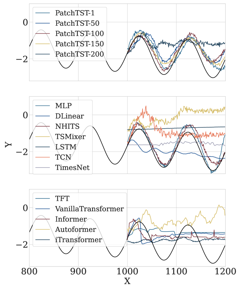
(b) Subtraction

Figure 3: Model time series forecasts for addition (a) and subtraction (b) composition tasks.

The PatchTST model excels at forecasting the composition of time series, particularly for addition and subtraction tasks as shown in Fig 2, outperforming all other evaluated Transformer models. However, the model’s performance on these tasks is sensitive to patch length, as shown in Fig. 3(a) in Appendix 4, indicating the critical role of patch length in the model’s knowledge manipulation capabilities.

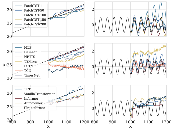
Figure 4: Model time series forecasts for the inverse search task.

Table 2 includes Mean Absolute Error (MAE) computed across all points within the forecast horizon and averaged across series for each task for DLinear, NHITS, and Transformer models. As shown in Table 2, DLinear had the smallest forecasting error for addition and subtraction composition tasks as well as comparison tasks, while NHITS had the smallest error for multiplication composition, function composition, and inverse search tasks. Results for each task, including standard deviations, for all 15 models are shown in Tables 4, 5, and 5 in Appendix 4. These tables also include baseline results for models trained on the first 1000 samples of OOD data. Example forecasts for composition and inverse search tasks are shown in Figs. 3 and 4 in Appendix 4. MAE formulation is provided in A.5.

Table 2: Mean Absolute Error (MAE) computed across all forecast points within the specified time horizon and averaged across series for each task. Best results are in bold, second-best in blue.

Model	Composition				Comparison	Inverse Search
	Add.	Sub.	Mult.	Func.
DLinear	0.689	0.935	10.522	21.155	1.072	0.539
NHITS	1.427	2.36	2.065	3.868	2.218	0.214
VanillaTransformer	2.432	2.993	8.249	11.291	2.120	0.551
TFT	1.024	3.243	13.395	10.159	2.045	0.574
Autoformer	1.708	3.999	12.845	13.383	3.966	1.180
Informer	2.045	3.025	9.246	12.268	2.131	0.877
iTransformer	1.358	2.994	15.197	31.632	2.885	1.164
PatchTST	1.717	2.168	3.497	6.209	1.740	0.394

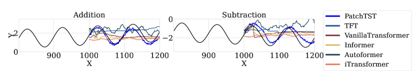
Figure 2: PatchTST shows strong capability in generating forecasts that accurately capture the composition of trend and seasonality series compared to other Transformer models.

5 Discussion

Our findings suggest that linear, MLP-based, and patch-based Transformer models, like PatchTST, offer implicit reasoning capabilities beyond memorization. PatchTST demonstrates strong OOD forecasting performance, supporting the use of patching input time series in TSFMs like MOMENT, Moirai, and TimesFM. Moreover, NHITS’s robust performance across tasks highlights the value of signal decomposition and hierarchical architectures, which if incorporated in future TSFMs could potentially enhance their forecasting capabilities. Our evaluation also shows the need for metrics beyond traditional loss measures. For example, despite TFT’s second-best MAE in addition composition, it forecasts a straight line as shown in Fig. 2, demonstrating the limitations of loss functions in capturing forecast pattern quality in complex tasks.

Appendix A Supplemental Information

A.1 Extended Related Work

Implicit Reasoning in LLMs.

Prior research has explored implicit reasoning in language models [2, 1, 27, 22, 29]. Implicit reasoning is often assessed through tasks that require models to apply knowledge learned during training to new test instances. One common form is composition, or multi-hop reasoning, where models must chain multiple facts to answer a question [22, 29, 27]. Other forms of implicit reasoning explored include comparison and inverse search [2, 1]. Comparison involves models making judgments about unseen or altered data, such as comparing attributes of entities from training. Inverse search tests the ability to retrieve information in the reverse order of the training task. An example of an inverse order task is identifying an entity based on its attributes when the model was trained for the reverse task. Allen-Zhu et al. [1] found that generative models struggle with inverse search unless pretrained for it specifically. [1].

While models can recall individual facts well, they struggle with multi-hop reasoning that requires ‘chain-of-thought’ logic. Yang et al. [27] found evidence of latent multi-hop reasoning for specific fact compositions, but noted it is highly contextual. Wang et al. demonstrated that Transformers can learn implicit reasoning, but only after extended training beyond typical overfitting thresholds [22]. Composition tasks have also been studied in machine translation, testing whether models can generalize learned command components to new conjunctions, such as repeating actions [11].

A.2 Models

Multi Layer Perceptrons (MLP) - A neural network architecture composed of stacked Fully Connected Neural Networks trained with backpropagation [14, 8, 18].

Neural Hierarchical Interpolation for Time Series (NHITS) - A deep learning model that applies multi-rate input pooling, hierarchical interpolation, and backcast residual connections together to generate additive predictions with different signal bands [5].

Long Short-Term Memory Recurrent Neural Network (LSTM) - A recurrent neural network (RNN) architecture that transforms hidden states from a multi-layer LSTM encoder into contexts which are used to generate forecasts using MLPs [19].

Temporal Convolution Network (TCN) - A 1D causal-convolutional network architecture that transforms hidden states into contexts which are used as inputs to MLP decoders to generate forecasts. Causal convolutions are used to generate contexts by convolving the prediction at time $t$ only with elements from time $t$ and earlier [4, 20].

TimesNet (TimesNet) - A deep learning architecture that transforms the original 1D time series into a set of 2D tensors based on multiple periods to capture intra- and inter-period variations modeled by 2D kernels [26].

VanillaTransformer (VanillaTransformer) - An encoder-decoder architecture with a multi-head attention mechanism that uses autoregressive features from a convolution network, window-relative positional embeddings from harmonic functions, and absolute positional embeddings from calendar data. An MLP decoder outputs time series predictions in a single pass [21, 30].

Temporal Fusion Transformer (TFT) - An attention-based deep learning architecture that learns temporal relationships at different scales using LSTMs for local processing and self-attention layers to model long-term dependencies. It also leverages variable selection networks and a series of gating layers to suppress unnecessary processing in the architecture [12].

Autoformer (Autoformer) - An encoder-decoder architecture with a multi-head attention mechanism that uses autoregressive features from a convolution network and absolute positional embeddings from calendar data. Decomposed trend and seasonal components are obtained using a moving average filter and an Auto-Correlation mechanism is used to identify periodic dependencies and aggregate similar sub-series [25, 21].

Informer (Informer) - An encoder-decoder architecture with a multi-head attention mechanism that has three key features: a ProbSparse self-attention mechanism with $O(L\log L)$ complexity, a self-attention distilling process, and an MLP decoder that outputs time-series predictions in a single pass. It uses autoregressive features from a convolution network, window-relative positional embeddings from harmonic functions, and absolute positional embeddings from calendar data [30, 21].

iTransformer (iTransformer) - An attention-based deep learning architecture that applies attention and feed-forward networks to inverted dimensions by embedding time points into variate tokens. The attention mechanism capture multivariate correlations while the feed-forward network learns nonlinear representations for each token [13].

Patch Time Series Transformer (PatchTST) - An encoder-only, multi-head attention-based architecture that separates input time series into sub-series level patches as input tokens. Each channel is dedicated to a single univariate time series, and all channels use the same embedding and Transformer weights. [15]

LagLlama (LagLlama) [17] - A foundation model for univariate probabilistic time series forecasting based on a decoder-only Transformer architecture that uses lags as covariates [17]. We use pretrained model weights from the HuggingFace library [23]. We use a context length of 32, as this is the parameter value on which the model was trained. Although the model can handle other context lengths, which may improve forecasting performance.

Chronos (Chronos) - A family of pretrained time series forecasting models that creates token sequences through scaling and quantization for input to a language model. Probabilistic forecasts are generated by sampling future trajectories from historical data [3]. We use the ‘t5-efficient-small’ pretrained model weights from the HuggingFace library [23].

MOMENT (MOMENT) - MOMENTis a family of foundation models for time series that uses an attention-based architecture and processes input time series into fixed-length patches with each mapped to a D-dimensional embedding. During pretraining, patches are masked to minimize reconstruction error, and a separate linear projection is trained to adapt embeddings for long-horizon forecasting and other tasks [10]. We use the ‘MOMENT-1-large’ pretrained model weights from the HuggingFace library [23].

TimesFM (TimesFM) - An attention-based decoder-only Transformer architecture that leverages input time series patching, masked causal attention, and sequential patch output predictions, with flexible output patch size [7]. We use the ‘timesfm-1.0-200m’ pretrained model weights from the HuggingFace library [23].

A.3 Synthetic Data Parameters

We leverage open-source code from MOMENT [10] to generate synthetic sinusoidal time series with varying trend, frequency, baseline, and amplitude. We use the following parameter values for all implicit reasoning tasks: $A\in[1,32]$, $B\in[3,32]$, $C\in[-32,32]$. $D\in[1,32]$ was used for addition, subtraction, and multiplication composition tasks, as well as for inverse search tasks. $D\in[-32,32]$ was used for function composition and comparison tasks. For composition tasks, we generate $n=30$ in-distribution (ID) series with evenly spaced parameter values. For comparison tasks, we generate $n=300$ ID series with evenly spaced parameter values. For the inverse search task, we generate $n=900$ ID addition composition aggregates using $n=30$ trend and seasonality series, each with evenly spaced parameter values.

A.4 Model Training and Parameters

We train models with the following parameters outlined in Table 3 to ensure consistent evaluation across architectures.

Table 3: Common hyperparameter search space

Hyperparameter	Considered Values
Input size	200
Learning rate	1e-3
Batch size	4
Windows batch size	256
Dropout	0.0
Training steps	2000
Validation check steps	50
Early stop patience steps	5
Random seed	0
Patch Length	DiscreteRange(1, 50, 100, 150, 200)
Hidden size	128
Model layers	3

A.5 Metrics

We use Mean Absolute Error (MAE) to evaluate model performance. Here, $H$ refers to the forecast horizon, $t$ refers to the time point at which forecasts are generated, $y$ refers to the target signal values, and $\hat{y}$ refers to the model;s predicted values:

$$MAE(y_{t+1,t+H},\hat{y}_{t+1,t+H})=\frac{1}{H}\sum_{i=t+1}^{t+H}|y_{i}-\hat{y}_{i}|.$$

Appendix B Supplemental Results

Table 4: Mean Absolute Error (MAE) averaged across series (standard deviation) for the composition implicit reasoning tasks: addition (add.), subtraction (sub.), multiplication (mult.), and sinusoidal function (function). MAE results for models trained on in-distribution (ID) time series and evaluated on out-of-distribution (OOD) series are presented in the ‘Task’ column. We also include baseline (base.) MAE results for models that are both trained and evaluated on OOD data. The best results are highlighted in bold, and the second best results are highlighted in blue.

Model	MAE
	Add.		Sub.		Mult.		Function
	Task	Base.	Task	Base.	Task	Base.	Task	Base.
MLP	1.604	0.386	2.637	0.350	2.097	1.507	10.099	2.730
	(1.173)	(0.284)	(1.648)	(0.197)	(1.559)	(1.127)	(6.372)	(2.3)
DLinear	0.689	0.743	0.935	0.715	10.522	8.792	21.155	10.653
	(0.349)	(0.333)	(0.452)	(0.333)	(7.945)	(5.284)	(23.965)	(6.783)
NHITS	1.427	0.216	2.36	0.184	2.065	1.194	3.868	1.736
	(1.089)	(0.132)	(1.489)	(0.215)	(1.687)	(0.813)	(2.207)	(1.547)
TSMixer	1.398	1.185	4.862	1.348	16.609	11.427	20.943	13.008
	(0.766)	(0.511)	(2.167)	(0.651)	(9.531)	(7.569)	(16.653)	(7.985)
LSTM	7.546	2.973	8.992	5.216	9.831	5.641	11.353	5.095
	(4.288)	(1.793)	(4.954)	(2.904)	(5.529)	(3.714)	(5.12)	(2.928)
TCN	5.716	2.538	5.063	3.057	8.359	2.606	11.413	4.123
	(3.228)	(1.432)	(2.597)	(1.667)	(4.816)	(1.995)	(4.781)	(2.391)
TimesNet	1.630	0.555	2.937	0.512	10.635	2.082	11.643	3.744
	(0.627)	(0.238)	(1.519)	(0.239)	(7.88)	(1.692)	(8.352)	(3.076)
VanillaTransformer	2.432	0.721	2.993	0.658	8.249	5.032	11.291	7.341
	(1.468)	(0.228)	(1.69)	(0.152)	(4.939)	(3.492)	(7.334)	(4.552)
TFT	1.024	0.709	3.243	1.057	13.395	5.121	10.159	6.548
	(0.408)	(0.295)	(1.507)	(0.504)	(9.688)	(3.834)	(5.228)	(4.455)
Autoformer	1.708	0.914	3.999	1.188	12.845	9.69	13.383	11.344
	(0.952)	(0.315)	(1.886)	(0.52)	(7.764)	(5.716)	(8.018)	(6.846)
Informer	2.045	0.741	3.025	0.78	9.246	5.423	12.268	10.335
	(1.273)	(0.235)	(1.702)	(0.28)	(5.303)	(3.4)	(8.89)	(5.724)
iTransformer	1.358	0.933	2.994	0.947	15.197	14.618	31.632	11.773
	(0.886)	(0.384)	(1.403)	(0.447)	(10.35)	(8.732)	(16.823)	(6.882)
PatchTST	1.717	0.435	2.168	0.584	3.497	1.600	6.209	7.231
	(1.113)	(0.285)	(1.185)	(0.404)	(2.442)	(1.108)	(4.009)	(6.031)
TSFMs	Zero-shot Forecasting
LagLlama	5.181		4.263		9.904		17.684
	(2.720)		(2.475)		(5.795)		(7.206)
Chronos	1.064		1.124		1.922		2.332
	(1.133)		(1.228)		(2.499)		(2.596)
TimesFM	0.475		0.467		0.355		0.672
	(0.375)		(0.457)		(0.336)		(0.655)
MOMENT	4.829		5.013		9.677		11.263
	(2.721)		(2.728)		(5.444)		(5.019)

Table 5: Model forecast Mean Absolute Error (MAE) averaged across series (standard deviation). MAE results for models trained on in-distribution (ID) time series and evaluated on out-of-distribution (OOD) series are presented in the ‘Task’ column. We also include baseline (base.) MAE results for models that are both trained and evaluated on OOD data. The best results are highlighted in bold, and the second best results are highlighted in blue.

(a) Comparison Task

Model	MAE
	Comparison
	Task	Base.
MLP	2.492	1.945
	(4.831)	(4.138)
DLinear	1.072	1.342
	(1.173)	(1.848)
NHITS	2.218	1.750
	(4.113)	(3.749)
TSMixer	2.488	2.391
	(3.371)	(3.570)
LSTM	3.174	4.663
	(3.767)	(5.571)
TCN	2.467	2.913
	(3.002)	(3.591)
TimesNet	3.570	1.972
	(6.309)	(4.001)
VanillaTransformer	2.120	2.040
	(4.071)	(4.066)
TFT	2.045	1.986
	(3.802)	(3.864)
Autoformer	3.966	3.785
	(5.097)	(5.145)
Informer	2.131	1.999
	(3.805)	(3.674)
iTransformer	2.885	3.106
	(4.052)	(4.429)
PatchTST	1.740	1.204
	(3.084)	(2.678)
TSFMs	Zero-Shot
LagLlama	5.307
	(7.512)
Chronos	0.704
	(1.362)
TimesFM	0.413
	(0.775)
MOMENT	3.414
	(3.915)

(b) Inverse Search Task

Model	MAE
	Inverse Search
	Task	Base.
MLP	0.632	0.076
	(0.523)	(0.040)
DLinear	0.539	0.444
	(0.433)	(0.389)
NHITS	0.214	0.035
	(0.231)	(0.055)
TSMixer	1.622	1.431
	(0.697)	(0.647)
LSTM	1.784	4.161
	(1.617)	(4.665)
TCN	1.666	3.113
	(1.444)	(3.504)
TimesNet	0.646	0.438
	(0.384)	(0.385)
VanillaTransformer	0.551	0.279
	(0.531)	(0.248)
TFT	0.574	0.961
	(0.464)	(0.504)
Autoformer	1.180	0.804
	(0.527)	(0.335)
Informer	0.877	0.436
	(0.425)	(0.210)
iTransformer	1.164	1.143
	(0.507)	(0.560)
PatchTST	0.394	0.293
	(0.545)	(0.195)
TSFMs	Zero-Shot
LagLlama	2.656
	(2.724)
Chronos	0.096
	(0.088)
TimesFM	0.070
	(0.075)
MOMENT	2.775
	(2.914)

(a) Addition

References

- Allen-Zhu and Li [2023] Zeyuan Allen-Zhu and Yuanzhi Li. Physics of language models: Part 3.2, knowledge manipulation. 2023.
- Allen-Zhu and Li [2024] Zeyuan Allen-Zhu and Yuanzhi Li. Physics of language models: Part 3.1, knowledge storage and extraction. In Proceedings of the 41st International Conference on Machine Learning, page 235, 2024.
- Ansari et al. [2024] Abdul Fatir Ansari, Lorenzo Stella, Caner Turkmen, Xiyuan Zhang, Pedro Mercado, Huibin Shen, Oleksandr Shchur, Syama Sundar Rangapuram, Sebastian Pineda Arango, Shubham Kapoor, Jasper Zschiegner, Danielle C. Maddix, Hao Wang, Michael W. Mahoney, Kari Torkkola, Andrew Gordon Wilson, Michael Bohlke-Schneider, and Yuyang Wang. Chronos: Learning the language of time series. 2024.
- Bai et al. [2018] Shaojie Bai, J. Zico Kolter, and Vladlen Koltun. An empirical evaluation of generic convolutional and recurrent networks for sequence modeling, 2018.
- Challu et al. [2022] Cristian Challu, Kin G. Olivares, Boris N. Oreshkin, Federico Garza, Max Mergenthaler-Canseco, and Artur Dubrawski. N-HiTS: Neural hierarchical interpolation for time series forecasting. In AAAI-23, 2022.
- Chen et al. [2023] Si-An Chen, Chun-Liang Li, Nathanael C. Yoder, Sercan Ö. Arık, and Tomas Pfister. TSMixer: An all-MLP architecture for time series forecasting. In Published in Transactions on Machine Learning Research, 2023.
- Das et al. [2024] Abhimanyu Das, Weihao Kong, Rajat Sen, and Yichen Zhou. A decoder-only foundation model for time-series forecasting. 2024.
- Fukushima [1975] Kunihiko Fukushima. Cognitron: A self-organizing multilayered neural network. Biol. Cybernetics, 20:121––136, 1975.
- Garza and Mergenthaler-Canseco [2023] Azul Garza and Max Mergenthaler-Canseco. TimeGPT-1, 2023.
- Goswami et al. [2024] Mononito Goswami, Konrad Szafer, Arjun Choudhry, Yifu Cai, Shuo Li, and Artur Dubrawski. MOMENT: A family of open time-series foundation models. In 41st International Conference on Machine Learning, 2024.
- Lake and Baroni [2018] Brenden M. Lake and Marco Baroni. Generalization without systematicity: On the compositional skills of sequence-to-sequence recurrent networks. In Proceedings of the 35th International Conference on Machine Learning, 2018.
- Lim et al. [2021] Bryan Lim, Sercan Ö. Arık, Nicolas Loeff, and Tomas Pfister. Temporal fusion transformers for interpretable multi-horizon time series forecasting. International Journal of Forecasting, 37(4):1748–1764, 2021.
- Liu et al. [2024] Yong Liu, Tengge Hu, Haoran Zhang, Haixu Wu, Shiyu Wang, Lintao Ma, and Mingsheng Long. iTransformer: Inverted transformers are effective for time series forecasting, 2024.
- Nair and Hinton [2010] Vinod Nair and Jeoffrey E. Hinton. Rectified linear units improve restricted boltzmann machines. In ICML-23, 2010.
- Nie et al. [2023] Yuqi Nie, Nam H. Nguyen, and Phanwadee Sinthong an Jayant Kalagnanam2. A time series is worth 64 words: Long-term forecasting with transformers. In Proceedings of the 11th International Conference on Learning Representations, 2023.
- Olivares et al. [2022] Kin G. Olivares, Cristian Challú, Federico Garza, Max Mergenthaler Canseco, and Artur Dubrawski. NeuralForecast: User friendly state-of-the-art neural forecasting models. PyCon Salt Lake City, Utah, US 2022, 2022. URL https://github.com/Nixtla/neuralforecast.
- Rasul et al. [2024] Kashif Rasul, Arjun Ashok, Andrew Robert Williams, Hena Ghonia, Rishika Bhagwatkar, Arian Khorasani, Mohammad Javad Darvishi Bayazi, George Adamopoulos, Roland Riachi, Nadhir Hassen, Marin Biloš, Sahil Garg, Anderson Schneider, Nicolas Chapados, Alexandre Drouin, Valentina Zantedeschi, Yuriy Nevmyvaka, and Irina Rish. Lag-Llama: Towards foundation models for probabilistic time series forecasting, 2024.
- Rosenblatt [1958] Frank Rosenblatt. The perceptron: A probabilistic model for information storage and organization in the brain. Psychological Review, 65(6):386––408, 1958.
- Sak et al. [2014] Haşim Sak, Andrew Senior, and Françoise Beaufays. Long short-term memory based recurrent neural network architectures for large vocabulary speech recognition, 2014.
- van den Oord et al. [2016] Aaron van den Oord, Sander Dieleman, Heiga Zen, Karen Simonyan, Oriol Vinyals, Alex Graves, Nal Kalchbrenner, Andrew Senior, and Koray Kavukcuoglu. WaveNet: A generative model for raw audio, 2016.
- Vaswani et al. [2017] Ashish Vaswani, Noam Shazeer, Niki Parmar, Jakob Uszkoreit, Llion Jones, and Aidan N. Gomez. Attention is all you need, 2017.
- Wang et al. [2024] Boshi Wang, Xiang Yue, Yu Su, and Huan Sun. Grokked transformers are implicit reasoners: A mechanistic journey to the edge of generalization. 2024.
- Wolf et al. [2020] Thomas Wolf, Lysandre Debut, Victor Sanh, Julien Chaumond, Clement Delangue, Anthony Moi, Pierric Cistac, Tim Rault, Rémi Louf, Morgan Funtowicz, Joe Davison, Sam Shleifer, Patrick von Platen, Clara Ma, Yacine Jernite, Julien Plu, Canwen Xu, Teven Le Scao, Sylvain Gugger, Mariama Drame, Quentin Lhoest, and Alexander M. Rush. Transformers: State-of-the-art natural language processing. In Proceedings of the 2020 Conference on Empirical Methods in Natural Language Processing: System Demonstrations, pages 38–45, Online, October 2020. Association for Computational Linguistics. URL https://www.aclweb.org/anthology/2020.emnlp-demos.6.
- Woo et al. [2024] Gerald Woo, Chenghao Liu, Akshat Kumar, Caiming Xiong, Silvio Savarese, and Doyen Sahoo. Unified training of universal time series forecasting transformers. In Proceedings of the 41st International Conference on Machine Learning, 2024.
- Wu et al. [2021] Haixu Wu, Jiehui Xu, Jianmin Wang, and Mingsheng Long. Autoformer: Decomposition transformers with auto-correlation for long-term series forecasting, 2021.
- Wu et al. [2023] Haixu Wu, Tengge Hu, Yong Liu, Hang Zhou, Jianmin Wang, and Mingsheng Long. TimesNet: Temporal 2d-variation modeling for general time series analysis. In Proceedings of the 34th International Conference on Learning Representations, 2023.
- Yang et al. [2024] Sohee Yang, Elena Gribovskaya, Nora Kassner, Mor Geva, and Sebastian Riedel. Do large language models latently perform multi-hop reasoning? arXiv preprint arXiv:2402.16837, 2024.
- Zeng et al. [2023] Ailing Zeng, Muxi Chen, Lei Zhang, and Qiang Xu. Are transformers effective for time series forecasting? In Proceedings of the AAAI Conference on Artificial Intelligence, 2023.
- Zhong et al. [2023] Zexuan Zhong, Zhengxuan Wu, Christopher D Manning, Christopher Potts, and Danqi Chen. MQuAKE: Assessing knowledge editing in language models via multi-hop questions. arXiv preprint arXiv:2305.14795, 2023.
- Zhou et al. [2021] Haoyi Zhou, Shanghang Zhang, Jieqi Peng, Shuai Zhang, Jianxin Li, Hui Xiong, and Wancai Zhang. Informer: Beyond efficient transformer for long sequence time-series forecasting, 2021.