Evaluating and Improving the Robustness of LiDAR-based Localization and Mapping

Abstract

LiDAR is one of the most commonly adopted sensors for simultaneous localization and mapping (SLAM) and map-based global localization. SLAM and map-based localization are crucial for the independent operation of autonomous systems, especially when external signals such as GNSS are unavailable or unreliable. While state-of-the-art (SOTA) LiDAR SLAM systems could achieve 0.5% (i.e., 0.5m per 100m) of errors and map-based localization could achieve centimeter-level global localization, it is still unclear how robust they are under various common LiDAR data corruptions.

In this work, we extensively evaluated five SOTA LiDAR-based localization systems under 18 common scene-level LiDAR point cloud data (PCD) corruptions. We found that the robustness of LiDAR-based localization varies significantly depending on the category. For SLAM, hand-crafted methods are in general robust against most types of corruption, while being extremely vulnerable (up to +80% errors) to a specific corruption. Learning-based methods are vulnerable to most types of corruptions. For map-based global localization, we found that the SOTA is resistant to all applied corruptions. Finally, we found that simple Bilateral Filter denoising effectively eliminates noise-based corruption but is not helpful in density-based corruption. Re-training is more effective in defending learning-based SLAM against all types of corruption.

I Introduction

Robotics and automation systems have been gaining significant prevalence in this decade. Of those, robots, drones, and autonomous vehicles have been making the news [1] due to their widespread adoption and related safety concerns [2].

Localization is fundamental to these systems since it keeps track of the position of a robotic system within an environment. Outdoors, and Global Navigation Satellite Systems (GNSS) are widely used for localization. In contrast, in urban, tunnel, and indoor settings where GNSS is hindered by weak satellite signals [3], simultaneous localization and mapping (SLAM) systems are favored since they operate independently of external signals and reliably navigate both indoors and outdoors. For these reasons, SLAM is widely used for locating and mapping-related tasks in robotics and autonomous driving. SLAM methods utilize either a camera, LiDAR, or a combination of both, with the optional integration of an Inertial Measurement Unit (IMU) [4]. Compared to vision SLAM, LiDAR SLAM has higher mapping accuracy, and better stability, is less susceptible to lighting conditions, and does not observe scale drift. These advantages lead to its popularity in large-scale use cases and facilitate more research and application in this direction.

Despite the recent successes of LiDAR SLAM, many challenges remain. Laser signals are robust under clear conditions, however, they decay significantly in rainy and foggy weather [5], making LiDAR SLAM degrade in adverse weather conditions [4]. Noise commonly occurs in point cloud data due to hardware limitations, motion, lighting, dust, or reflective surface [6, 7, 8, 9, 10, 11]. Also, mechanical, solid-state, and phased-array LiDAR sensors are built differently and SLAM designed for one may not be interchangeable with others [4]. Instability causes localization to miscalculate a deviation from the agent’s current position. Depending on the scale of the deviation, it can cause automated vehicles to drive off-road or onto the wrong lane. In robotic systems, it would result in the wake-up or kidnapped robot problem, since the large gap between the two consecutive frames’ positions can cause the robot to be unable to recover, i.e., either it stops due to failed localization or reset and initiates a costly recovery and relocalize process, discarding the learned map/knowledge [12, 13, 14].

Such challenges to the LiDAR sensor raise concerns about the performance of SLAM in diverse environments [4]. To this end, there is a lack of comprehensive evaluation on the manifestation and impact of such issues on LiDAR SLAM. Moreover, increasing efforts invested in learning-based SLAM raises additional robustness concerns due to DNNs’ sensitivity to noises [15, 16, 17]. Yet there is a lack of comparative evaluation in that regard. Hence in this work, we evaluate the robustness of such applications against common LiDAR data corruption due to adverse weather, noisy environments, and losses. Once the effects are discovered, we want to explore whether current defense strategies such as re-training and denoising are sufficient to address these issues.

Our contributions can be summarized as follows:

• We propose a novel framework to evaluate the robustness of the SOTA LiDAR-based localization against common LiDAR data corruptions. To the best of our knowledge, this is the first work to study this problem.

• We study the effectiveness of common defense strategies, such as denoising and re-training, against common LiDAR data corruption.

• We share our code and data publicly.

II Background and related works

LiDAR-based localization can either simultaneously build a map and localize the agent within it, i.e., SLAM [4], or localize the agent within a pre-built map, i.e., global localization [18].

II-A LiDAR-based localization and mapping

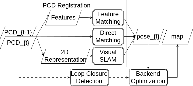
Figure 1: Different types of LiDAR SLAM Overview.

LiDAR-based localization is the most accurate, stable, resistant to different lighting conditions, and has no scale drift, thus suitable for large-scale applications [4]. It could be used from autonomous driving [19, 20], robot exploration [21] to deep space exploration [22]. LiDAR-based localization can be roughly categorized into LiDAR-only SLAM, MSF-based SLAM, and map-based global localization.

II-A1 LiDAR-only SLAM

LiDAR-only SLAM can be categorized into feature-based, direct, and projection-based methods as shown in Figure 1. Feature-based methods [23, 24] extract appearance, geometric, semantics, or shape-based features for scan matching. Alternatively, direct methods [25, 26] match the scan directly via handcrafted point cloud registration methods, neural networks, or a map. Finally, projection-based approaches [27, 28] convert the point cloud to a 2D representation and leverage existing visual SLAM methods. The effectiveness of these methods is highly dependent on the environments, equipment, and platforms. Traditional SLAM frameworks use hand-crafted features or models [29, 30, 31, 32, 33] to register scans. In contrast, learning-based SLAM [34, 35, 25], facilitated by the development of 3D computer vision, extracts features and register scans automatically. Due to the focus on computer vision, these methods only focus on feature extraction and scan registration rather than a complete solution. Moreover, their accuracy, stability, and performance leave much to be desired [4]. In our work, we look to evaluate the robustness of LiDAR-only SLAM.

II-A2 MSF-based SLAM

On the other hand, LiDAR can be incorporated into an MSF-based SLAM. MSF SLAM combines the output from the LiDAR with camera, IMU, and GNSS, to complement each other and improve localization performance [4, 36]. These methods build upon the LiDAR-only solutions. They are not included in this study.

II-A3 Map-based LiDAR Localization

Map-based localization registers an online LiDAR scan with a pre-built map and tries to locate it within the map [18, 37, 38, 39, 40, 41]. This offers precise and efficient localization, which is especially useful in safety-critical systems such as autonomous driving systems [42, 43]. However, these methods require a pre-built map, which is typically created using the SLAM algorithm offline and may require ground truth information to improve the map quality. Map-based localization shares many common technologies with LiDAR-only SLAM (e.g., LiDAR scan registration), so we will also attempt to evaluate the robustness of such systems.

II-B Robustness of LiDAR-based Systems

Previous works evaluated the impact of data corruption on LiDAR-based 3D obstacle detection. This includes benchmarking against perturbations [44, 45, 46, 47, 48]; testing and adversarial attacks via point-based [49, 50, 51, 52, 53, 54, 55, 56, 57] and object spoofing methods [58, 59, 60, 61, 62, 63, 64]. Finally, complex weather simulators [65, 66, 67, 68] model LiDAR’s interaction with dense droplets as well as how light bounces off objects under rain, snow, and fog. Many of these works are tailored to objects and thus inapplicable to localization. Hence, in this work, we evaluate LiDAR-based localization against a set of applicable perturbations.

III Methodology

In this section, we describe our framework for evaluating and improving the robustness of LiDAR-based localization.

Category	Perturbation Type
Weather	rain, snow, rain + wet ground (rain_wg),
	snow + wet ground (snow_wg), fog
Noise	background noise (bg_noise), upsample,
	uniform noise in CCS (uni_noise),
	gaussian noise in CCS (gau_noise),
	impulse noise in CCS (imp_noise),
	uniform noise in SCS (uni_noise_rad),
	uniform noise in SCS (gau_noise_rad),
	uniform noise in SCS (imp_noise_rad),
Density	local density increase (local_inc),
	local density decrease (local_dec),
	beam deletion (beam_del),
	layer deletion (layer_del), cutout

TABLE I: The 18 perturbations used by our work from three categories. CCS refers to Cartesian Coordinate System and SCS refers to Spherical Coordinate System. The details will be introduced in Section III.

III-A Evaluating the Robustness of LiDAR SLAM

LiDAR SLAMs are deployed in complex and diverse environments which may impact the sensitivity of LiDAR. It is important to evaluate the robustness and reliability of such systems in various environments. Our framework employs a total of 18 perturbations on cloud corruptions to emulate diverse environments such as adverse weather conditions and equipment malfunctions. We select a comprehensive set of corruption reflecting commonly occurring phenomena that impact the entire LiDAR scan instead of individual objects. Table I summarizes the list of perturbation types.

Weather Perturbations. Adverse weather such as rain and snow can negatively affect the quality of LiDAR scans. Randomly distributed droplets in the air from rain, snow, and fog can scatter light and disturb the measurement of LiDAR, thus injecting noises into the resulting PCD. Furthermore, wet ground always co-occurs with rain and snow due to the precipitation, which will reflect differently from dry ground.

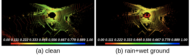
Figure 2: An example of rain and wet ground corruption. The field view and reflection intensities are significantly decayed compared to the clean data.

Our framework simulates the following weather conditions considering both the direct impact of weather conditions on LiDAR (e.g., droplets causing scattering), as well as impacts of wet grounds on LiDAR (e.g., reflections).

• Rain or Snow. We utilize an off-the-shelf weather simulator, i.e., LISA [65, 66] for simulating PCD under adverse weather such as rain and snow. LISA utilizes a physics-based model to simulate the decayed return of laser pulses in rain and snow weather, which is realistic as evaluated by previous work [47].

• Fog. We utilize a fog Simulation on Real LiDAR Point Clouds (FS) [67] to simulate fog. While LISA already has a fog perturbation, it is more general, and works such as FS provide a better fog simulation model without needing unavailable data such as optical channel information. Hence, we use FS for fog simulation. FS simulates the effect of fog on real-world LiDAR point clouds that have been recorded in clear weather. FS models fog by modifying the impulse response changes to reflect the impact of different fog densities on the environment and the surrounding objects.

• Rain + Wet Ground (rain_wg). We combine LISA and Wet Ground Model from [68] to produce a more realistic simulation than rain alone. The Wet Ground Model builds an optical model to simulate the reflection on the wet ground based on the thickness of the water. Figure 2 shows an example of this corruption.

• Snow + Wet Ground (snow_wg). Similar to rain + wet ground, we produce more realistic snow weather by combining LISA’s snow simulation and the wet ground model on PCD.

Noise Perturbations. Noises happen during LiDAR measurement due to internal (e.g., equipment vibration and measurement errors) or external (e.g., dust and background light) factors [11, 69, 70]. We design perturbations on PCDs to simulate the errors attributed to such internal and external factors.

Noise Type	Formula to Generate Noise
Gaussian (CCS)	$p_{i}+\Delta p*SEV,\;\Delta p\sim\mathcal{N}(0,1)^{3},p_{i}\in P$
Uniform (CCS)	$p_{i}+\Delta p*SEV,\;\Delta p\sim\mathcal{U}(-1,1)^{3},p_{i}\in P$
Impulse (CCS)	$p_{i}+\Delta p*C,\;\Delta p\sim\mathcal{U}\{-1,1\}^{3},$
	$p_{i}\in RS(P,SEV)$
Gaussian (SCS)	$p_{i}+\Delta r*SEV,\;\Delta r\sim\mathcal{N}(0,1),p_{i}\in P$
Uniform (SCS)	$p_{i}+\Delta r*SEV,\;\Delta r\sim\mathcal{U}(-1,1),p_{i}\in P$
Impulse (SCS)	$p_{i}+\Delta r*C,\;\Delta r\sim\mathcal{U}\{-1,1\},$
	$p_{i}\in RS(P,SEV)$
Background (CCS)	$P_{new}=P\cup\{p_{i}^{\prime}|j=1,2,...,SEV\}$
	$p_{i}^{\prime}=\{x_{i}^{\prime},y_{i}^{\prime},z_{i}^{\prime}\},\left\{\begin{array}[]{l}x_{i}^{\prime}\sim\mathcal{U}(x_{\min},x_{\max})\\ y_{i}^{\prime}\sim\mathcal{U}(y_{\min},y_{\max})\\ z_{i}^{\prime}\sim\mathcal{U}(z_{\min},z_{\max})\\ \end{array}\right.$
Upsample (CCS)	$P_{new}=P\cup\{p_{i}+\Delta p|\Delta p\sim\mathcal{U}(-0.1,0.1),$
	$p_{i}\in RS(P,SEV)\}$

TABLE II: Noise-based corruptions. SEV (severity) refers to the significance of corruption, whose definition varies based on the type of corruption. C refers to a constant value, whose concrete value varies in different places. RS refers to a random subset function, which samples a subset from the input based on the given $SEV$. $\Delta p$ refers to a point in CCS, so $+\Delta p$ means we change the three coordinates in CCS. $\Delta r$ refers to the range value, $+\Delta r$ means we only change the range value in SCS.

We show the details of noise perturbations in Table II. One frame of PCD is annotated as $P=\{p_{i}|i=1,2,...N\}$, where $N$ is the number of points in the point cloud. We apply three distributions of noises (Gaussian, Uniform, and Impulse) to two coordinate systems (Cartesian and Spherical, CCS and SCS for short) to emulate different noise sources. In CCS, one point is represented by $p=\{x,y,z\}$, i.e., Euclidean distance to each planes, while in SCS, one point is represented by $p=\{r,\phi,\theta\}$, where $r$ is the range, i.e., Euclidean distance from the origin to the point, $\phi$ is the azimuthal angle and $\theta$ is the polar angle. Noises in CCS represent inaccuracies caused by the vibration or rotating of the sensor [48] while SCS can better represent inaccurate measurement of time of flight (ToF) [47].

In addition to re-positioning existing PCD points, we synthesize new points to emulate environment noises, such as dust in the air, through background noise and upsample applied to CCS. Background noise adds points randomly in the entire space, while upsample adds points close to randomly selected points.

Density Perturbations.

Corruption	Formula to Generate Noise
Local Inc	$P_{new}=P\cup P_{add},$
	$P_{add}=\bigcup_{i=0}^{SEV}IP(NN_{100}(p_{i}))$
Local Dec	$P_{new}=P\setminus P_{rm},$
	$P_{rm}=\bigcup_{i=0}^{SEV}RS(NN_{100}(p_{i}),C)$
Cutout	$P_{new}=P\setminus\bigcup_{i=0}^{SEV}NN_{20}(p_{i})$
Beam Del	$P_{new}=RS(P,SEV)$
Layer Del	$P_{new}=P\setminus\bigcup_{i\in S}Layer_{i},$
	$S=RS(\{1,2,...64\},SEV),P=\bigcup_{i=1}^{64}Layer_{i}$

TABLE III: Density-based corruptions. SEV (severity) refers to the significance of corruption, whose definition varies based on the type of corruption. C refers to a constant value, whose concrete value varies in different places. IP refers to the 3D interpolation function. $NN_{k}$ refers to the k-nearest neighbor function. RS refers to a random subset function, which samples a subset from the input based on the given number.

The density of points can be changed due to internal (e.g., malfunction of the equipment) or external (e.g., occlusion between objects and reflection on object surface) factors [71, 72]. We simulate five density-related corruptions, local density increase, local density decrease, cutout, beam deletion, and layer deletion. The definitions of these corruptions are listed in Table III.

III-B Improving the Robustness of LiDAR SLAM

Re-training. Learning-based systems are data-driven and could learn to fit themselves into a data distribution. We expect these systems to learn how to handle the corrupted data by themselves through re-training, which is a common enhancement and defensive strategy for deep learning [65, 67, 68, 73, 74].

Denoising. Handcraft algorithms are expected to be tuned and adapted by experts once inefficiencies are identified. Therefore such improvements are achieved case by case and lack of generality. Hence in this work, for non-learning-based SLAM, we focus on denoising the data, which is a more general way. Point cloud denoising removes unwanted noises from LiDAR scans to improve their quality. There are three categories of denoising, i.e., filter, optimization, and deep learning-based, each with its advantages and disadvantages [11]. In this work, we adopted a filter-based method, i.e., the bilateral filter by [75], which is reliable, and significantly faster than the alternatives while preserving the intensity with readily available implementation.

IV Experiment Setup

IV-A Subject LiDAR SLAM Systems

TABLE IV: Subject Systems. The errors are reported based on our replication.

Category	Dataset	Year	Method	Error
SLAM	MULLS [76]	2021	Feature-based	0.56%
	KISS-ICP [77]	2023	Direct	0.51%
	DeLORA [78]	2021	Projection-based	7.78%
	NeRF-LOAM [79]	2023	Distance Field	1.70%
Map-based
Localization	LocNDF [37]	2023	Distance Field	0.059m

We experiment four SOTA LiDAR SLAM techniques and one map-based LiDAR localization, as shown in Table IV. We try to select one representative work from different types of mainstream LiDAR localization technologies, i.e. feature-based, direct, and projection-based methods [4]. We also include two neural distance field-based approaches, which have emerged and become popular since the success of the NeRF [80] in computer vision.

MULLS [76] is a feature-based SLAM that uses ground filtering and principal components analysis to extract features from the PCD. It builds local sub-maps using previous PCD and match the current frame with local sub-maps by the proposed multi-metric linear least square iterative closest point algorithm to compute the pose. KISS-ICP [77] is a direct SLAM that combines point-to-point ICP with adaptive thresholding, a robust kernel, universal motion compensation, and point cloud subsampling. DeLORA [78] is a projection-based, unsupervised SLAM. It projects the 3D point cloud to 2D image representations and employs ResNet to extract features from the 2D image. Then it predicts the translation and rotation by feeding the features into an MLP. NeRF-LOAM employs a neural network to predict the signed distance field (SDF). It first builds the previous frames into an octree. Then it samples intersected points between laser rays and voxels in the previously built octree. Given sampled points, the neural network predicts the SDF. Since sampled points are transformed to the same coordinate system as the previously built octree by the pose to be estimated, NeRF-LOAM optimizes the pose, neural network, and voxel embedding jointly by minimizing the loss between predicted SDF and real SDF. Different from NeRF-LOAM, LocNDF trains a neural network offline to predict the SDF. Given the online LiDAR scan, it tries to find a pose $P$ so that the neural network can produce minimal SDF when sampled points are transformed by $P$.

IV-B Datasets

We use KITTI Visual Odometry/SLAM Evaluation 2012 (KITTI) [19] to evaluate the four SLAM systems, DeLORA, MULLS, KISS-ICP, and NeRF-LOAM. KITTI 00 to 10 sequences are released with ground truths. We conducted our experiment on sequences 09 and 10 because (1) DeLORA was trained on sequences 00-08 hence only 09 and 10 remain. (2) sequences 09 and 10 are of moderate sizes which facilitate the large number of perturbations in a reasonable amount of time and computation resources.

Apollo South-Bay [81] contains completed ADS recordings covering various driving scenarios. In this work, we used a subset of ColumbiaPark-3, consisting of 700 testing frames, which is consistent with LocNDF’s pre-trained model [37].

IV-C Evaluation Metrics

For the evaluation of the precision of SLAMs, we adopted the relative pose error (RPE) [19]. RPE is widely used in previous work [4] to measure and compare the performance of SLAM. RPE is calculated as:

$$RPE_{rot}(\mathscr{F})=\frac{1}{|\mathscr{F}|}\sum_{(i,j)\in\mathscr{F}}\angle[(\hat{p}_{j}\ominus\hat{p}_{i})\ominus(p_{j}\ominus p_{i})]$$ (1)

$$RPE_{trans}(\mathscr{F})=\frac{1}{|\mathscr{F}|}\sum_{(i,j)\in\mathscr{F}}||(\hat{p}_{j}\ominus\hat{p}_{i})\ominus(p_{j}\ominus p_{i})||_{2}$$ (2)

where $RPE_{trans}$ measures the relative translation error and $RPE_{rot}$ measures the relative rotation error between the estimated pose and the ground truth, $\mathscr{F}$ is a set of frames $(i,j)$, $\hat{p}$ is the estimated pose and $p$ is the ground truth pose, $\ominus$ is the inverse compositional operator [82] and $\angle[\cdot]$ is the rotation angle.

V Experiment Results

V-A Robustness Results of LiDAR SLAM

Method. We applied our robustness framework to evaluate the subject SLAM systems (Table IV). We first perturb the KITTI and Apollo-SouthBay datasets with the corruptions in Table I. Note that NeRF-LOAM is computationally expensive (i.e., requiring at least 24GB GPU memory and days to finish KITTI for one of the 18 perturbations), we took a statistically-significant sample of frames from KITTI for NeRF-LOAM as a proof of concept.

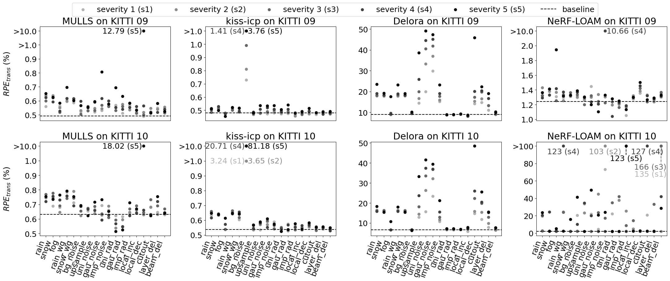
Figure 3: Performance of each system on corrupted KITTI LiDAR Odometry Sequence 09 and 10. Errors with significantly different magnitudes from the majority are aligned at their magnitude and the actual values are labeled in the figure. For example, an error of 12.79% is aligned to “$>$10.0”. If multiple errors overlap at the same magnitude, we label the two highest severity levels.

Results. We show the results of RPE_trans in Figures 3. Due to the space limitation, we do not present the RPE_rot in the paper as it is correlated with RPE_trans. We share the detailed results of RPE_rot in our public artifact.

For the non-learning SLAM systems, we find that they have degraded performance on almost all kinds of LiDAR perturbed data compared to the baseline (i.e., un-perturbed data). Furthermore, each SLAM system is vulnerable to a particular type of perturbation, where their performance drops significantly. The error of MULLS increases from below 0.5% to up to 0.8%. Even worse, the error of MULLS with “local density decrease” (severity 5) increased to more than 12% for KITTI 09 and 18% for KITTI 10 from 0.5%, which is more than 100 times worse. Similarly, kiss-icp is especially vulnerable to “background noise”. While the error only increased by less than 0.2% in most cases, the error of kiss-icp caused by background noise increases up to 80% (with severity 5 on KITTI 10) from less than 0.6% RPE_trans. Moreover, even the lightest background noise (severity 1) causes a significant error increase from less than 0.6% to more than 3% RPE_trans on KITTI 10.

We observe different results for the learning-based SLAM, Delora and NeRF-LOAM. Delora is vulnerable to most perturbations, especially those related to noise. The RPE_trans error increases from less than 10 percent to tens of percent (up to 50%). Lastly, NeRF-LOAM is quite different from others. We find the results differ very much between the two KITTI sequences, indicating that NeRF-LOAM’s robustness results highly depend on data. In KITTI 09, NeRF-LOAM is not sensitive to most perturbations except for one. While in KITTI 10, NeRF-LOAM is shown to be highly sensitive in most cases. Also, interestingly, in many cases, it shows better robustness with a higher severity than a lower severity. For example, for the cutout perturbation on KITTI 10, NeRF-LOAM performs poorly with severity 4, however, the performance is very well and much higher with severity 5 which is close to the baseline with the clean data. NeRF-LOAM is optimizing a mini-network online for tens of iterations. We hypothesize that the poor results are because NeRF-LOAM is far from being optimized in tens of iterations for these cases.

For the map-based localization system LocNDF, our evaluation shows that it is very robust against all types of corruptions. The map-based SLAM LocNDF is robust, at the cost of significant upfront investments (in terms of multiple scans of the environment to build the LiDAR map) and its inability to work in unexplored environments.

V-B Improving the Robustness of LiDAR SLAM

Method. We only concern MULLS, kiss-icp, and Delora in this denoising experiment, since LocNDF is robust against all kinds of corruption, while NeRF-LOAM could not produce consistent results between different trials on the same data. Firstly, we apply the Bilateral Filter to denoise the corrupted data and then re-run all the localization algorithms on the denoised data. Furthermore, since Delora uses a learning-based approach, we augment Delora’s training set (i.e., KITTI 00 to 08 sequences) by applying our proposed LiDAR corruptions and re-train Delora on the augmented data.

We focus on denoising the most representative corruption types that affect the algorithms most, i.e., local density decrease (MULLS and Delora), background noise (kiss-icp), uniform noise (Delora), Gaussian noise (Delora), and rain/snow (moderate effects on all systems). We denoise these types of corruption at severity 1, 3, and 5. We also denoise the clean data to see if the denoising has side effects on clean data.

Similarly, we fine-tune Delora on the corruptions that affect it most significantly, namely, rain, snow, fog, upsample, uniform noise, Gaussian noise, impulse noise, local density decrease, cutout, and layer deletion. We only augmented the training data with these corruptions at severity 5 and fine-tuned Delora for 6 epochs with the default training hyper-parameters.

Results.

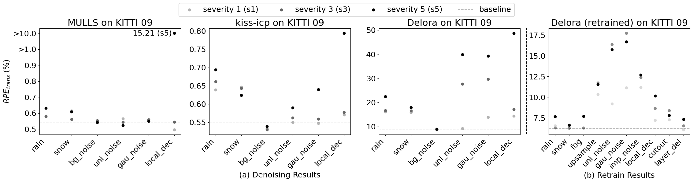
Figure 4: (a) Performance on the denoised data. (b) Performance of the retrained model.

We present the performance of the three systems on the denoised data for KITTI 09 in Figure 4 (a). The results on KITTI 10 are available in our replication package due to the space limitation. For MULLS, local density decrease (local_dec) at severity 5 is the corruption that affects it most significantly. We find that the errors even increased by 2.43% after denoising. Besides, we find that denoising could reduce the error by 0.26% for Gaussian noise. The changes are insignificant for the remaining cases (less than 0.1%).

For kiss-icp, background noise (bg_noise) is the corruption that affects it most significantly. We find that the denoising can reduce the error by 0.2% (severity 1) to 3.22% (severity 5), that is, the negative effect of the corruption is fully eliminated (we observed the same effects on KITTI 10, where the errors at severity 5 are reduced by 80%). However, the denoising causes the errors on rain and snow to increase by 0.13% to 0.18%, and on local density decrease at severity 5 to increase by 0.28%. The changes are insignificant for the remaining cases.

For Delora, we find that denoising can reduce its errors in most cases including the baseline, by 0.44% to 16.08%. Similar to MULLS and kiss-icp, we find that the errors in local density decrease (local_dec) increased by 2.74%.

We present the performance of the Delora after fine-turning for KITTI 09 in Figure 4 (b). We find that re-training can bring a much higher improvement than denoising: the errors are reduced by 2.73% to 35.79% for the baseline and all types of corruption. However, for KITTI 10, despite the overall effects being similar, we observed a slight increase in the errors for the baseline and a few corruptions. It is important to note that our fine-tuning was relatively naive: we only augmented KITTI 00 to 08 with the selected corruptions at severity 5 and used the original learning rate. We believe that further improvements could be achieved by a more refined fine-tuning process, such as augmenting the dataset with the corruption at different severities, and adjusting the learning rate and the ratio between clean and corrupted data.

VI conclusion

In this work, we extensively evaluated the robustness of the LiDAR-based localization systems, including SLAM and map-based localization. Our results revealed that all kinds of SOTA LiDAR-based SLAM systems are vulnerable to specific types of LiDAR data corruption. We further showed that simple Bilateral Filter denoising can effectively eliminate noise-based data corruptions, however, the density-based corruptions remain unsolved. We also showed that the data augmentation with corrupted data can improve the robustness of the learning-based LiDAR SLAM significantly, and is even beneficial to its performance on clean data.

VII Acknowledgement

We would like to express our gratitude to our interns, Marko Griesser-Aleksic, Ali Ouabou El Ghoulb, and Hanchong Qiu, for their invaluable assistance and contribution to this project.

References

- [1] VOA, “Robot begins removing fukushima nuclear plant’s melted fuel,” 2024. [Online]. Available: https://www.voanews.com/a/robot-begins-removing-fukushima-nuclear-plant-s-melted-fuel/7781166.html
- [2] Forbes, “93% have concerns about self-driving cars according to new forbes legal survey,” 2024. [Online]. Available: https://www.forbes.com/advisor/legal/auto-accident/perception-of-self-driving-cars/
- [3] P. Shi, Q. Ye, and L. Zeng, “A novel indoor structure extraction based on dense point cloud,” ISPRS International Journal of Geo-Information, vol. 9, no. 11, 2020.
- [4] Y. Zhang, P. Shi, and J. Li, “3d lidar slam: A survey,” The Photogrammetric Record, vol. 39, pp. 457 – 517, 2024.
- [5] R. H. Rasshofer, M. Spies, and H. Spies, “Influences of weather phenomena on automotive laser radar systems,” Advances in Radio Science, vol. 9, pp. 49–60, 2011.
- [6] M. Hongchao and W. Jianwei, “Analysis of positioning errors caused by platform vibration of airborne lidar system,” 2012 8th IEEE International Symposium on Instrumentation and Control Technology (ISICT) Proceedings, pp. 257–261, 2012.
- [7] R. Wang, B. Wang, M. Xiang, C. Li, S. Wang, and C. Song, “Simultaneous time-varying vibration and nonlinearity compensation for one-period triangular-fmcw lidar signal,” Remote Sensing, vol. 13, no. 9, 2021.
- [8] L. Mona, Z. Liu, D. Müller, A. Omar, A. Papayannis, G. Pappalardo, N. Sugimoto, and M. Vaughan, “Lidar measurements for desert dust characterization: An overview,” Advances in Meteorology, vol. 2012, no. 1, p. 356265, 2012.
- [9] H. Chen and J. Shen, “Denoising of point cloud data for computer-aided design, engineering, and manufacturing,” Engineering with Computers, vol. 34, pp. 523 – 541, 2017.
- [10] X.-F. Han, J. S. Jin, M.-J. Wang, W. Jiang, L. Gao, and L. Xiao, “A review of algorithms for filtering the 3d point cloud,” Signal Processing: Image Communication, vol. 57, pp. 103–112, 2017.
- [11] L. Zhou, G. Sun, Y. Li, W. Li, and Z. Su, “Point cloud denoising review: from classical to deep learning-based approaches,” Graphical Models, vol. 121, p. 101140, 2022.
- [12] I. Bukhori and Z. H. Ismail, “Detection of kidnapped robot problem in monte carlo localization based on the natural displacement of the robot,” International Journal of Advanced Robotic Systems, vol. 14, 2017.
- [13] Y. Seow, R. Miyagusuku, A. Yamashita, and H. Asama, “Detecting and solving the kidnapped robot problem using laser range finder and wifi signal,” in 2017 IEEE International Conference on Real-time Computing and Robotics (RCAR), 2017, pp. 303–308.
- [14] R. C. Luo, K. C. Yeh, and K. H. Huang, “Resume navigation and re-localization of an autonomous mobile robot after being kidnapped,” in 2013 IEEE International Symposium on Robotic and Sensors Environments (ROSE), 2013, pp. 7–12.
- [15] C. Szegedy, W. Zaremba, I. Sutskever, J. Bruna, D. Erhan, I. J. Goodfellow, and R. Fergus, “Intriguing properties of neural networks,” CoRR, vol. abs/1312.6199, 2013.
- [16] S.-M. Moosavi-Dezfooli, A. Fawzi, and P. Frossard, “Deepfool: A simple and accurate method to fool deep neural networks,” 2016 IEEE Conference on Computer Vision and Pattern Recognition (CVPR), pp. 2574–2582, 2015.
- [17] J. Zhang, M. Harman, L. Ma, and Y. Liu, “Machine learning testing: Survey, landscapes and horizons,” IEEE Transactions on Software Engineering, vol. 48, pp. 1–36, 2019.
- [18] H. Yin, X. Xu, S. Lu, X. Chen, R. Xiong, S. Shen, C. Stachniss, and Y. Wang, “A survey on global lidar localization: Challenges, advances and open problems,” International Journal of Computer Vision, pp. 1–33, 2024.
- [19] A. Geiger, P. Lenz, and R. Urtasun, “Are we ready for autonomous driving? the kitti vision benchmark suite,” in Conference on Computer Vision and Pattern Recognition (CVPR), 2012.
- [20] G. Wan, X. Yang, R. Cai, H. Li, Y. Zhou, H. Wang, and S. Song, “Robust and precise vehicle localization based on multi-sensor fusion in diverse city scenes,” in 2018 IEEE International Conference on Robotics and Automation (ICRA), 2018, pp. 4670–4677.
- [21] W. E. King, M. R. Zanetti, E. Hayward, and K. Miller, “The kinematic navigation and cartography knapsack (knack): Demonstrating slam (simultaneous localization and mapping) lidar as a tool for exploration and mapping of lunar pits and caves,” in 2023 4th International Planetary Caves Conference, 2023.
- [22] K. M. Miller, A. Draffen, B. Robinson, B. Steiner, J. Walters, P. Bremner, J. L. Jetton, B. De, L. Santiago, E. Hayward, and M. Zanetti, “Knack-slam: Kinematic navigation and cartography knapsack velocity-aided lidar inertial simultaneous localization and mapping (slam),” in 2022 53rd Lunar and Planetary Science Conference, 2022.
- [23] H. Wang, C. Wang, and L. Xie, “Intensity-slam: Intensity assisted localization and mapping for large scale environment,” IEEE Robotics and Automation Letters, vol. 6, pp. 1715–1721, 2021.
- [24] K. Honda, K. Koide, M. Yokozuka, S. Oishi, and A. Banno, “Generalized loam: Lidar odometry estimation with trainable local geometric features,” IEEE Robotics and Automation Letters, vol. 7, no. 4, pp. 12 459–12 466, 2022.
- [25] B. Zhou, Y. Tu, Z. Jin, C. Xu, and H. Kong, “Hpplo-net: Unsupervised lidar odometry using a hierarchical point-to-plane solver,” IEEE Transactions on Intelligent Vehicles, vol. 9, no. 1, pp. 2727–2739, 2024.
- [26] I. Vizzo, T. Guadagnino, B. Mersch, L. Wiesmann, J. Behley, and C. Stachniss, “Kiss-icp: In defense of point-to-point icp – simple, accurate, and robust registration if done the right way,” IEEE Robotics and Automation Letters, vol. 8, pp. 1029–1036, 2022.
- [27] J. Liu, G. Wang, C. Jiang, Z. Liu, and H. Wang, “Translo: A window-based masked point transformer framework for large-scale lidar odometry,” in AAAI Conference on Artificial Intelligence, 2023.
- [28] X. Zheng and J. Zhu, “Efficient lidar odometry for autonomous driving,” IEEE Robotics and Automation Letters, vol. 6, pp. 8458–8465, 2021.
- [29] J. Zhang and S. Singh, “Low-drift and real-time lidar odometry and mapping,” Autonomous Robots, vol. 41, pp. 401–416, 2017.
- [30] T. Shan and B. Englot, “Lego-loam: Lightweight and ground-optimized lidar odometry and mapping on variable terrain,” in 2018 IEEE/RSJ International Conference on Intelligent Robots and Systems (IROS), 2018, pp. 4758–4765.
- [31] J. Lin and F. Zhang, “Loam livox: A fast, robust, high-precision lidar odometry and mapping package for lidars of small fov,” 2020 IEEE International Conference on Robotics and Automation (ICRA), pp. 3126–3131, 2019.
- [32] H. Wang, C. Wang, and L. Xie, “Intensity-slam: Intensity assisted localization and mapping for large scale environment,” IEEE Robotics and Automation Letters, vol. 6, no. 2, pp. 1715–1721, 2021.
- [33] P. Dellenbach, J.-E. Deschaud, B. Jacquet, and F. Goulette, “Ct-icp: Real-time elastic lidar odometry with loop closure,” 2022 International Conference on Robotics and Automation (ICRA), pp. 5580–5586, 2021.
- [34] Q. Li, S. Chen, C. Wang, X. Li, C. Wen, M. Cheng, and J. Li, “Lo-net: Deep real-time lidar odometry,” in 2019 IEEE/CVF Conference on Computer Vision and Pattern Recognition (CVPR), 2019, pp. 8465–8474.
- [35] G. Chen, B. Wang, X. Wang, H. Deng, B. Wang, and S. Zhang, “Psf-lo: Parameterized semantic features based lidar odometry,” in 2021 IEEE International Conference on Robotics and Automation (ICRA). IEEE Press, 2021, p. 5056–5062.
- [36] P. Groves, Principles of GNSS, Inertial, and Multisensor Integrated Navigation Systems, Second Edition. Artech, 2013.
- [37] L. Wiesmann, T. Guadagnino, I. Vizzo, N. Zimmerman, Y. Pan, H. Kuang, J. Behley, and C. Stachniss, “Locndf: Neural distance field mapping for robot localization,” IEEE Robotics and Automation Letters, vol. 8, no. 8, pp. 4999–5006, 2023.
- [38] P. Shi, J. Li, and Y. Zhang, “A fast lidar place recognition and localization method by fusing local and global search,” ISPRS Journal of Photogrammetry and Remote Sensing, 2023.
- [39] ——, “Lidar localization at 100 fps: A map-aided and template descriptor-based global method,” Int. J. Appl. Earth Obs. Geoinformation, vol. 120, p. 103336, 2023.
- [40] X. Chen, I. Vizzo, T. Läbe, J. Behley, and C. Stachniss, “Range image-based lidar localization for autonomous vehicles,” 2021 IEEE International Conference on Robotics and Automation (ICRA), pp. 5802–5808, 2021.
- [41] L. Wiesmann, R. Marcuzzi, C. Stachniss, and J. Behley, “Retriever: Point cloud retrieval in compressed 3d maps,” in 2022 International Conference on Robotics and Automation (ICRA), 2022, pp. 10 925–10 932.
- [42] Baidu, “Apollo localization module documentation,” 2024. [Online]. Available: https://github.com/ApolloAuto/apollo/tree/master/modules/localization
- [43] T. IV, “Autoware localization module documentation,” 2024. [Online]. Available: https://github.com/autowarefoundation/autoware.universe/tree/main/localization/
- [44] K. Yu, T. Tao, H. Xie, Z. Lin, T. Liang, B. Wang, P. Chen, D. Hao, Y. Wang, and X. Liang, “Benchmarking the robustness of lidar-camera fusion for 3d object detection,” in 2023 IEEE/CVF Conference on Computer Vision and Pattern Recognition Workshops (CVPRW), 2023, pp. 3188–3198.
- [45] X. Gao, Z. Wang, Y. Feng, L. Ma, Z. Chen, and B. Xu, “Benchmarking robustness of ai-enabled multi-sensor fusion systems: Challenges and opportunities,” Proceedings of the 31st ACM Joint European Software Engineering Conference and Symposium on the Foundations of Software Engineering, 2023.
- [46] F. Albreiki, S. Abughazal, J. Lahoud, R. M. Anwer, H. Cholakkal, and F. S. Khan, “On the robustness of 3d object detectors,” Proceedings of the 4th ACM International Conference on Multimedia in Asia, 2022.
- [47] S. Li, Z. Wang, F. Juefei-Xu, Q. Guo, X. Li, and L. Ma, “Common corruption robustness of point cloud detectors: Benchmark and enhancement,” IEEE Transactions on Multimedia, pp. 1–12, 2023.
- [48] Y. Dong, C. Kang, J. Zhang, Z. Zhu, Y. Wang, X. Yang, H. Su, X. Wei, and J. Zhu, “Benchmarking robustness of 3d object detection to common corruptions,” in Proceedings of the IEEE/CVF Conference on Computer Vision and Pattern Recognition, 2023, pp. 1022–1032.
- [49] Z. Q. Zhou and L. Sun, “Metamorphic testing of driverless cars,” Commun. ACM, vol. 62, no. 3, p. 61–67, feb 2019.
- [50] S. Zheng, W. Liu, S. Shen, Y. Zang, C. Wen, M. Cheng, and C. Wang, “Adaptive local adversarial attacks on 3d point clouds,” Pattern Recognition, vol. 144, p. 109825, 2023.
- [51] X. Xu, J. Zhang, Y. Li, Y. Wang, Y. Yang, and H. T. Shen, “Adversarial attack against urban scene segmentation for autonomous vehicles,” IEEE Transactions on Industrial Informatics, vol. 17, pp. 4117–4126, 2021.
- [52] J. Sun, Y. Cao, Q. A. Chen, and Z. M. Mao, “Towards robust lidar-based perception in autonomous driving: General black-box adversarial sensor attack and countermeasures,” in Proceedings of the 29th USENIX Conference on Security Symposium, ser. SEC’20. USA: USENIX Association, 2020.
- [53] Y. Zhu, C. Miao, T. Zheng, F. Hajiaghajani, L. Su, and C. Qiao, “Can we use arbitrary objects to attack lidar perception in autonomous driving?” in Proceedings of the 2021 ACM SIGSAC Conference on Computer and Communications Security, ser. CCS ’21. New York, NY, USA: Association for Computing Machinery, 2021, p. 1945–1960.
- [54] Y. Zhu, C. Miao, F. Hajiaghajani, M. Huai, L. Su, and C. Qiao, “Adversarial attacks against lidar semantic segmentation in autonomous driving,” Proceedings of the 19th ACM Conference on Embedded Networked Sensor Systems, 2021.
- [55] Z. Xiong, H. Xu, W. Li, and Z. Cai, “Multi-source adversarial sample attack on autonomous vehicles,” IEEE Transactions on Vehicular Technology, vol. 70, no. 3, pp. 2822–2835, 2021.
- [56] B. Liu, Y. Guo, J. Jiang, J. Tang, and W. Deng, “Multi-view correlation based black-box adversarial attack for 3d object detection,” in Proceedings of the 27th ACM SIGKDD Conference on Knowledge Discovery & Data Mining, ser. KDD ’21. New York, NY, USA: Association for Computing Machinery, 2021, p. 1036–1044.
- [57] X. Wang, M. Cai, F. Sohel, N. Sang, and Z. Chang, “Adversarial point cloud perturbations against 3d object detection in autonomous driving systems,” Neurocomputing, vol. 466, pp. 27–36, 2021.
- [58] Y. Cao, C. Xiao, B. Cyr, Y. Zhou, W. Park, S. Rampazzi, Q. A. Chen, K. Fu, and Z. M. Mao, “Adversarial sensor attack on LiDAR-based perception in autonomous driving,” in Proceedings of the 2019 ACM SIGSAC Conference on Computer and Communications Security. ACM, nov 2019.
- [59] H. Shin, D. Kim, Y. Kwon, and Y. Kim, “Illusion and dazzle: Adversarial optical channel exploits against lidars for automotive applications,” in Cryptographic Hardware and Embedded Systems – CHES 2017, W. Fischer and N. Homma, Eds. Cham: Springer International Publishing, 2017, pp. 445–467.
- [60] Y. Cao, N. Wang, C. Xiao, D. Yang, J. Fang, R. Yang, Q. A. Chen, M. Liu, and B. Li, “Invisible for both camera and lidar: Security of multi-sensor fusion based perception in autonomous driving under physical-world attacks,” in 2021 IEEE Symposium on Security and Privacy (SP), May 2021, pp. 176–194.
- [61] M. Abdelfattah, K. Yuan, Z. J. Wang, and R. Ward, “Towards universal physical attacks on cascaded camera-lidar 3d object detection models,” in 2021 IEEE International Conference on Image Processing (ICIP), 2021, pp. 3592–3596.
- [62] K. Yang, T. Tsai, H. Yu, M. Panoff, T.-Y. Ho, and Y. Jin, “Robust roadside physical adversarial attack against deep learning in lidar perception modules,” Proceedings of the 2021 ACM Asia Conference on Computer and Communications Security, 2021.
- [63] J. Tu, H. Li, X. Yan, M. Ren, Y. Chen, M. Liang, E. Bitar, E. Yumer, and R. Urtasun, “Exploring adversarial robustness of multi-sensor perception systems in self driving,” in Proceedings of the 5th Conference on Robot Learning, ser. Proceedings of Machine Learning Research, A. Faust, D. Hsu, and G. Neumann, Eds., vol. 164. PMLR, 08–11 Nov 2022, pp. 1013–1024.
- [64] J. Tu, M. Ren, S. Manivasagam, M. Liang, B. Yang, R. Du, F. Cheng, and R. Urtasun, “Physically realizable adversarial examples for lidar object detection,” in Proceedings of the IEEE/CVF Conference on Computer Vision and Pattern Recognition (CVPR), June 2020.
- [65] V. Kilic, D. Hegde, V. Sindagi, A. B. Cooper, M. A. Foster, and V. M. Patel, “Lidar light scattering augmentation (lisa): Physics-based simulation of adverse weather conditions for 3d object detection,” arXiv preprint arXiv:2107.07004, 2021.
- [66] D. Hegde, V. Kilic, V. Sindagi, A. B. Cooper, M. Foster, and V. M. Patel, “Source-free unsupervised domain adaptation for 3d object detection in adverse weather,” in 2023 IEEE International Conference on Robotics and Automation (ICRA). IEEE, 2023, pp. 6973–6980.
- [67] M. Hahner, C. Sakaridis, D. Dai, and L. Van Gool, “Fog Simulation on Real LiDAR Point Clouds for 3D Object Detection in Adverse Weather,” in IEEE International Conference on Computer Vision (ICCV), 2021.
- [68] M. Hahner, C. Sakaridis, M. Bijelic, F. Heide, F. Yu, D. Dai, and L. Van Gool, “LiDAR Snowfall Simulation for Robust 3D Object Detection,” in IEEE/CVF Conference on Computer Vision and Pattern Recognition (CVPR), 2022.
- [69] H. Ma and J. Wu, “Analysis of positioning errors caused by platform vibration of airborne lidar system,” in 2012 8th IEEE International Symposium on Instrumentation and Control Technology (ISICT) Proceedings, 2012, pp. 257–261.
- [70] C. Deng, L. Pan, C. Wang, X. Gao, W. Gong, and S. Han, “Performance analysis of ghost imaging lidar in background light environment,” Photon. Res., vol. 5, no. 5, pp. 431–435, Oct 2017.
- [71] Q. Xu, Y. Zhong, and U. Neumann, “Behind the curtain: Learning occluded shapes for 3d object detection,” in Proceedings of the AAAI Conference on Artificial Intelligence, vol. 36, no. 3, 2022, pp. 2893–2901.
- [72] S. Uttarkabat, S. Appukuttan, K. Gupta, S. Nayak, and P. Palo, “Bloomnet: Perception of blooming effect in adas using synthetic lidar point cloud data,” in 2024 IEEE Intelligent Vehicles Symposium (IV), 2024, pp. 1886–1892.
- [73] I. J. Goodfellow, J. Shlens, and C. Szegedy, “Explaining and harnessing adversarial examples,” arXiv preprint arXiv:1412.6572, 2014.
- [74] A. Xiao, J. Huang, D. Guan, K. Cui, S. Lu, and L. Shao, “Polarmix: A general data augmentation technique for lidar point clouds,” in Advances in Neural Information Processing Systems, S. Koyejo, S. Mohamed, A. Agarwal, D. Belgrave, K. Cho, and A. Oh, Eds., vol. 35. Curran Associates, Inc., 2022, pp. 11 035–11 048. [Online]. Available: https://proceedings.neurips.cc/paper˙files/paper/2022/file/475b85eb74d201bead9927807e713e95-Paper-Conference.pdf
- [75] J. Digne and C. de Franchis, “The Bilateral Filter for Point Clouds,” Image Processing On Line, vol. 7, pp. 278–287, 2017.
- [76] Y. Pan, P. Xiao, Y. He, Z. Shao, and Z. Li, “Mulls: Versatile lidar slam via multi-metric linear least square,” in 2021 IEEE International Conference on Robotics and Automation (ICRA), 2021, pp. 11 633–11 640.
- [77] I. Vizzo, T. Guadagnino, B. Mersch, L. Wiesmann, J. Behley, and C. Stachniss, “Kiss-icp: In defense of point-to-point icp – simple, accurate, and robust registration if done the right way,” IEEE Robotics and Automation Letters, vol. 8, no. 2, pp. 1029–1036, 2023.
- [78] J. Nubert, S. Khattak, and M. Hutter, “Self-supervised learning of lidar odometry for robotic applications,” in 2021 IEEE International Conference on Robotics and Automation (ICRA), 2021, pp. 9601–9607.
- [79] J. Deng, Q. Wu, X. Chen, S. Xia, Z. Sun, G. Liu, W. Yu, and L. Pei, “Nerf-loam: Neural implicit representation for large-scale incremental lidar odometry and mapping,” in Proceedings of the IEEE/CVF International Conference on Computer Vision (ICCV), October 2023, pp. 8218–8227.
- [80] B. Mildenhall, P. P. Srinivasan, M. Tancik, J. T. Barron, R. Ramamoorthi, and R. Ng, “Nerf: Representing scenes as neural radiance fields for view synthesis,” in ECCV, 2020.
- [81] W. Lu, Y. Zhou, G. Wan, S. Hou, and S. Song, “L3-net: Towards learning based lidar localization for autonomous driving,” in Proceedings of the IEEE Conference on Computer Vision and Pattern Recognition, 2019, pp. 6389–6398.
- [82] R. Kümmerle, B. Steder, C. Dornhege, M. Ruhnke, G. Grisetti, C. Stachniss, and A. Kleiner, “On measuring the accuracy of slam algorithms,” Autonomous Robots, vol. 27, pp. 387–407, 2009.