\makegloss

Simple robust two-stage estimation and inference
for generalized impulse responses and multi-horizon causalityaaa  This work was supported by the William Dow Chair in Political Economy (McGill University), the Social Sciences and Humanities Research Council of Canada, and the Fonds de recherche sur la société et la culture (Québec).

Jean-Marie Dufour
McGill University and Endong Wang
McGill University
  William Dow Professor of Economics, McGill University, Centre interuniversitaire de recherche en analyse des organisations (CIRANO), and Centre interuniversitaire de recherche en économie quantitative (CIREQ). Mailing address: Department of Economics, McGill University, Leacock Building, Room 414, 855 Sherbrooke Street West, Montréal, Québec H3A 2T7, Canada. TEL: (1) 514 398 6071; FAX: (1) 514 398 4800; e-mail: =jean-marie.dufour@mcgill.ca= . Web page: http://www.jeanmariedufour.com  Department of Economics, McGill University, Montréal, Québec H3A2T7, Canada. TEL: (1) 514 772 7078; e-mail: =endong.wang@mail.mcgill.ca= . Web page: http://www.endongwang.com
(First version: February 2023
Revised: March 2024
This version: July 2024
Compiled: , \texttime )
Abstract

This paper introduces a novel two-stage estimation and inference procedure for generalized impulse responses (GIRs). GIRs encompass all coefficients in a multi-horizon linear projection model of future outcomes of $y$ on lagged values (Dufour and Renault, 1998), which include the Sims’ impulse response. The conventional use of Least Squares (LS) with heteroskedasticity- and autocorrelation-consistent covariance estimation is less precise and often results in unreliable finite sample tests, further complicated by the selection of bandwidth and kernel functions. Our two-stage method surpasses the LS approach in terms of estimation efficiency and inference robustness. The robustness stems from our proposed covariance matrix estimates, which eliminate the need to correct for serial correlation in the multi-horizon projection residuals. Our method accommodates non-stationary data and allows the projection horizon to grow with sample size. Monte Carlo simulations demonstrate our two-stage method outperforms the LS method. We apply the two-stage method to investigate the GIRs, implement multi-horizon Granger causality test, and find that economic uncertainty exerts both short-run (1-3 months) and long-run (30 months) effects on economic activities.

Keywords. Multi-horizon projection model; Generalized impulse response; Causality; Two-stage estimation; Statistical inference;

JEL   classification: C3; C12; C15; C53.

List of Definitions, Assumptions, Propositions and Theorems

\@starttoc

lth

1 Introduction

The concept of causality introduced by \citeasnounwiener1956theory and \citeasnoungranger1969investigating, often referred to as Granger causality, constitutes a foundational approach for studying dynamic relationships between time series. While \citeasnoungranger1969investigating primarily focused on bivariate causality at a single horizon, the concept was generalized by \citeasnoundufour1998short to account for multi-horizon causality.222For related work, see also \citeasnounsims1980macroeconomics, \citeasnounhsiao1982autoregressive, and \citeasnounlutkepohl1993testing. This extension serves two purposes. First, Granger causality at one horizon may not fully capture the causal dynamics in a multivariate system, as causality at one horizon does not necessarily imply causality at multiple horizons.333An example from \citeasnoundufour1998short: In a trivariate system ($x,y,z$), $x_{t}$ may not Granger-cause $y_{t}$ at time $t$, but $x_{t}$ might still help predict $y_{t}$ several periods ahead through indirect effects mediated by $z_{t}$. For instance, $x_{t}$ could predict $z_{t}$ one period ahead, which in turn affects $y_{t}$ at a later time. Second, the concept of impulse response proposed by \citeasnounsims1980macroeconomics has limitations, as a zero impulse response is neither a necessary nor sufficient condition for non-causality in the sense of Wiener and Granger (see \citeasnoundufour1993relationship). To address the issue of non-causality between two vectors of variables across multiple horizons in the presence of auxiliary variables, \citeasnoundufour1998short introduced a necessary and sufficient condition on the coefficients in a multi-horizon linear projection model. These coefficients, referred to as “generalized impulse responses” (GIRs), include Sims’ impulse response as a special case. In this paper, we propose an innovative two-stage estimation method for the GIRs in a multi-horizon linear projection model444\citeasnoundufour2006short refer to this model as “autoregression at horizon $h$” or “($p,h$)-autoregression” within a finite lag VAR($p$) framework. The autoregression at horizon $h$ model is also referred to as ”Local Projection,” which is widely used to estimate impulse response functions due to its straightforward inference [see \citeasnounjorda2005estimation, \citeasnounmontiel2021local, and \citeasnounwolf2021same]., which complements two conventional methods: the recursive method and the Least Squares (LS) projection method.

The recursive method begins by estimating the VAR coefficients, followed by the recursive computation of GIRs, as these represent nonlinear transformations of the underlying VAR coefficients. Statistical tests for non-causality restrictions across multiple horizons (two or more) are expressed as zero constraints on multilinear forms involving the VAR coefficients. However, the Wald-type test criteria, can lead to asymptotically singular covariance matrices, making standard asymptotic theory inapplicable. This issue has been explored by \citeasnounlutkepohl1997modified, \citeasnounbenkwitz2000problems, \citeasnouninoue2020uniform, and \citeasnoundufour2023wald. To address this challenge, \citeasnounpelletier2004problems and \citeasnoundufour2006short implemented a multi-horizon linear projection model with LS estimation.555The multi-horizon linear projection model has gained considerable attention in economics and finance, particularly for forecasting, impulse response estimation, causality testing, and causality measurement. For related work, see \citeasnounfama1988dividend, \citeasnouncampbell1988dividend, \citeasnoundufour2010short, \citeasnoundufour2012measuring, \citeasnounzhang2016exchange, \citeasnounsalamaliki2019transmission, \citeasnounshi2020causal. Appropriate asymptotic inference for the coefficient estimators can be obtained through adjustments for serially correlated residuals, such as using heteroskedasticity and autocorrelation consistent (HAC) estimators. However, LS-based multi-horizon linear projection estimates may suffer from reduced estimation efficiency as the horizon lengthens, and the reliability of confidence intervals constructed with HAC standard error estimates can be fragile. For further discussion, see \citeasnoundufour2006short, \citeasnounkilian2011reliable, and \citeasnounmontiel2021local. Although \citeasnoundufour2006short proposed a closed-form formula for estimating the covariance matrix, they also cautioned that the finite-sample estimate may not always be positive semi-definite. Therefore, in this study, we conduct a comprehensive reevaluation of the estimation method and inference procedures for GIR coefficients, aiming to improve the reliability of covariance matrix estimates and potentially achieve more efficient coefficient estimates.

Our two-stage estimation method for GIRs makes five key contributions to the existing literature on multi-horizon linear projection and causality studies.

First, we introduce an innovative identification method for GIRs that leverages second-moment conditions of observables and VAR innovations. This novel approach offers an alternative to the traditional LS method for estimating multi-horizon linear projection models, drawing on the well-established Two-Stage Least Squares (2SLS) framework but diverging in its application. The method consists of two distinct stages: in the first, VAR residuals are estimated using LS, and in the second, these residuals are employed as instrumental variables in a 2SLS procedure. To address potential issues related to unit roots, we also incorporate a lag-augmented version of the two-stage estimation. Our approach complements the LS method in multi-horizon projection models, enhancing both estimation precision and the robustness of inference.

Second, we compare the estimation efficiency of our two-stage approach with the LS method through both theoretical and empirical analyses. The theoretical discussion is based on an illustrative AR(2) process, where we compare the asymptotic variances of the two methods using explicit formulas and the true values of the underlying data-generating process. This analysis shows that LS estimates outperform the two-stage estimates only when the horizon is very short or the data is highly cyclical. Empirically, we conduct Monte Carlo simulations on a bivariate VAR(2) process, which demonstrate that the two-stage estimates are generally no less efficient than LS estimates. Our findings serve as a reminder to the econometrics community that instrumental variable estimates in time series may not always suffer from efficiency loss compared to LS. Furthermore, our theoretical results show that the two-stage estimates are asymptotically as efficient as the lag-augmented two-stage estimates, contradicting the common belief that lag augmentation in time series typically reduces efficiency.

Third, we develop a simple and robust method for estimating the covariance matrix of GIR estimates, which relies on the long-run variance of the regression score function. This approach eliminates the need to correct for serial correlation in the projection error. Our method removes the necessity for HAC estimates for all coefficients in a multi-horizon linear projection, including those for impulse response functions and lagged coefficients. By bypassing the complications associated with selecting bandwidths and kernel functions in HAC estimation, our approach simplifies the process. Monte Carlo simulations show that our robust covariance estimates lead to more reliable empirical test results compared to HAC estimates.

Fourth, we contribute to econometric theory by deriving the asymptotic normality of two-stage GIR estimates uniformly over the parameter space, allowing the projection horizon to grow with the sample size. Specifically, we consider the persistence of underlying data processes to range from stationary to integrated of order one or order two. The projection horizon is permitted to expand infinitely at varying rates relative to the sample size, depending on the parameter space. This uniformity across the parameter space and allowance for long-range horizons provide robust theoretical justification for empirical macroeconomic applications.

Fifth, our empirical analysis of the GIRs for economic activity in response to economic uncertainty reveals both short-run (1–3 months) and long-run (around 30 months) causal effects. The findings underscore the longer-than-expected impact of uncertainty on economic activity. Additionally, our empirical GIR studies highlight the limitations of impulse response analysis. In the long run, the Wald test on impulse responses is statistically insignificant, while the causality test remains significant, suggesting that impulse responses may fail to capture persistent causal effects over extended horizons.

Relevant Literature–From an economic conceptual perspective, the multi-horizon linear projection model, as examined in this paper, forms a foundational framework in the study of causality and predictability \citeasnounlutkepohl1993testing, \citeasnoundufour1998short, \citeasnoundufour2006short, \citeasnoundufour2010short, \citeasnoundiebold2014network. The novel identification and estimation method we propose draws from innovation algorithms for (vector) ARMA processes \citeasnounhannan1982recursive, \citeasnounbrockwell1991time, \citeasnoundufour2022practical, and is closely related to recent literature on Local Projection-Instrumental Variable (LP-IV) methods, as explored by \citeasnounstock2018identification. To the best of our knowledge, no existing studies have focused on using estimated VAR residuals as internal instruments to estimate GIRs within a multi-horizon linear projection model.

Regarding the statistical inference of two-stage estimates, the methodology for obviating HAC standard errors, even in the presence of serially correlated residuals, has been explored by \citeasnounmontiel2021local, \citeasnounbreitung2023projection, and \citeasnounxu2023local. However, these studies primarily focus on Sims; impulse responses rather than all coefficients in the projection model. The concept of uniform inference, which controls the test level in the "worst" case scenario, is thoroughly discussed in \citeasnoundufour2003identification and \citeasnounandrews2020generic. Specific applications to time series can be found in \citeasnounmikusheva2007uniform, \citeasnounmikusheva2012one, \citeasnouninoue2020uniform, \citeasnounmontiel2021local, and \citeasnounxu2023local. Research on long (potentially infinite) projection horizons has also been conducted by \citeasnounmontiel2021local and \citeasnounxu2023local. Our paper is the first to fully examine uniform inference for all coefficient estimates in a multi-horizon linear projection model, while also addressing restrictions on the projection horizon for stationary, I(1), and I(2) processes.

Outline–Section 2 introduces the notation and outlines the data generation process. In Section 3, we present the concept of two-stage identification and estimation. Section 4 explores robust inference methods that eliminate the need to correct for serial correlation in the projection residuals. The main statistical results on uniform inference for two-stage estimates are detailed in Section 5. Section 6 compares the asymptotic efficiency of our two-stage estimates with standard LS estimates. Section 7 presents the results of Monte Carlo simulations. In Section 8, we apply the proposed statistical methodology for GIR estimation to analyze the dynamic causality of economic uncertainty on macroeconomic aggregates. Finally, we conclude the paper in Section 9.

2 Framework

2.1 Model and parameter space

In this paper, we consider a multivariate time series following a Vector Autoregressive (VAR) process,

$\displaystyle y_{t}=\Phi_{1}y_{t-1}+\Phi_{2}y_{t-2}+\cdots+\Phi_{p}y_{t-p}+{u}_{t}$ (2.1)

where ${y}_{t}$ represents a $K$-dimensional vector of variables, and ${u}_{t}$ is a vector of innovations. The sequence of ${u}_{t}$ is defined on a probability space $(\Omega,\mathcal{F},\mathbb{P})$. We define the information set at time $t$, denoted as $\mathcal{F}_{t}$, which is generated by $\{y_{s}\}_{s\leq t}$. We consider ${u}_{t}$ as a white noise vector process with non-singular covariance matrix $\Sigma_{u}$. The order $p$ is a finite integer known a priori.666Two reasons support the assumption that the order $p$ is known a priori. First, the VAR coefficient estimates still have pointwise convergence to a standard Gaussian distribution as long as order $p$ can be consistently estimated by certain types of information criteria (see p62, \citeasnounkilian2017structural). Second, in practice, order $p$ can be considered a known upper bound for the number of VAR lags. Thus, the assumption that $p$ is known a priori is not as restrictive as it might initially appear. For the sake of notation simplicity, we omit the intercept and deterministic function in our notation, which generally do not impact the limiting results for the estimated coefficients.777In practice, researchers may incorporate dummy variables or polynomial functions of time $t$ to “detrend” the data, as discussed in \citeasnountoda1995statistical. The initial conditions are set as $y_{t}=0$ for $-p+1\leq t\leq 0$.

We investigate a broad range of time series processes, including stationary processes, I(1), and I(2) processes. In addition, we account for the presence of a ’local-to-unit’ root, aiming to ensure uniform inference across the specified parameter space while allowing the projection horizon to grow infinitely. Our framework also accommodates the potential presence of cointegration within the process, further enhancing its practical applicability. Notably, we highlight that processes conforming to a VARX model can also benefit from our findings. This is because VARX is a specific case of VAR, where the equation for the exogenous variable imposes constraints on the coefficients of the endogenous variables, setting them to zero (see p. 74 in \citeasnounkilian2017structural).

We build up the following setup for the VAR parameter space definition:

Definition 2.1

VAR Parameter Space: Given $c=(c_{0},c_{1})^{\prime}$, $c_{0},c_{1}>0$, ${{}\mathchoice{\mbox{\boldmath$\displaystyle\mathchar 271\relax$}}{\mbox{\boldmath$\textstyle\mathchar 271\relax$}}{\mbox{\boldmath$\scriptstyle\mathchar 271\relax$}}{\mbox{\boldmath$\scriptscriptstyle\mathchar 271\relax$}}}\in(0,1)$, and integer ${{}\mathchoice{\mbox{\boldmath$\displaystyle\mathchar 270\relax$}}{\mbox{\boldmath$\textstyle\mathchar 270\relax$}}{\mbox{\boldmath$\scriptstyle\mathchar 270\relax$}}{\mbox{\boldmath$\scriptscriptstyle\mathchar 270\relax$}}}\in\{0,1,2\}$, let $\mathcal{B}({{}\mathchoice{\mbox{\boldmath$\displaystyle\mathchar 270\relax$}}{\mbox{\boldmath$\textstyle\mathchar 270\relax$}}{\mbox{\boldmath$\scriptstyle\mathchar 270\relax$}}{\mbox{\boldmath$\scriptscriptstyle\mathchar 270\relax$}}},c,{{}\mathchoice{\mbox{\boldmath$\displaystyle\mathchar 271\relax$}}{\mbox{\boldmath$\textstyle\mathchar 271\relax$}}{\mbox{\boldmath$\scriptstyle\mathchar 271\relax$}}{\mbox{\boldmath$\scriptscriptstyle\mathchar 271\relax$}}})$ denote the space of autoregressive coefficients such that the lag polynomial $\Phi_{{}\mathchoice{\mbox{\boldmath$\displaystyle\mathchar 270\relax$}}{\mbox{\boldmath$\textstyle\mathchar 270\relax$}}{\mbox{\boldmath$\scriptstyle\mathchar 270\relax$}}{\mbox{\boldmath$\scriptscriptstyle\mathchar 270\relax$}}}(L)=I_{K}-\sum_{i=1}^{p}\Phi_{i}L^{i}$ admits the factorization

$\displaystyle\Phi_{{}\mathchoice{\mbox{\boldmath$\displaystyle\mathchar 270\relax$}}{\mbox{\boldmath$\textstyle\mathchar 270\relax$}}{\mbox{\boldmath$\scriptstyle\mathchar 270\relax$}}{\mbox{\boldmath$\scriptscriptstyle\mathchar 270\relax$}}}(L)=B_{{{}\mathchoice{\mbox{\boldmath$\displaystyle\mathchar 270\relax$}}{\mbox{\boldmath$\textstyle\mathchar 270\relax$}}{\mbox{\boldmath$\scriptstyle\mathchar 270\relax$}}{\mbox{\boldmath$\scriptscriptstyle\mathchar 270\relax$}}}}(L)U_{1}(L)U_{2}(L)\Pi$ (2.2)

where ${{}\mathchoice{\mbox{\boldmath$\displaystyle\mathchar 277\relax$}}{\mbox{\boldmath$\textstyle\mathchar 277\relax$}}{\mbox{\boldmath$\scriptstyle\mathchar 277\relax$}}{\mbox{\boldmath$\scriptscriptstyle\mathchar 277\relax$}}}_{min}(\Pi)>c_{0}$, $U_{i}(L)=I-\mathbb{1}_{({{}\mathchoice{\mbox{\boldmath$\displaystyle\mathchar 270\relax$}}{\mbox{\boldmath$\textstyle\mathchar 270\relax$}}{\mbox{\boldmath$\scriptstyle\mathchar 270\relax$}}{\mbox{\boldmath$\scriptscriptstyle\mathchar 270\relax$}}}\geq i)}P_{i}L$, $P_{i}=\textup{diag}[{{}\mathchoice{\mbox{\boldmath$\displaystyle\mathchar 282\relax$}}{\mbox{\boldmath$\textstyle\mathchar 282\relax$}}{\mbox{\boldmath$\scriptstyle\mathchar 282\relax$}}{\mbox{\boldmath$\scriptscriptstyle\mathchar 282\relax$}}}_{m,i}]$, ${{}\mathchoice{\mbox{\boldmath$\displaystyle\mathchar 282\relax$}}{\mbox{\boldmath$\textstyle\mathchar 282\relax$}}{\mbox{\boldmath$\scriptstyle\mathchar 282\relax$}}{\mbox{\boldmath$\scriptscriptstyle\mathchar 282\relax$}}}_{m,i}\in[-1,1]$, for $1\leq m\leq K$ and $i=1,2$. In particular, it is restricted that $|{{}\mathchoice{\mbox{\boldmath$\displaystyle\mathchar 282\relax$}}{\mbox{\boldmath$\textstyle\mathchar 282\relax$}}{\mbox{\boldmath$\scriptstyle\mathchar 282\relax$}}{\mbox{\boldmath$\scriptscriptstyle\mathchar 282\relax$}}}_{m,2}|=1,\text{ if }|{{}\mathchoice{\mbox{\boldmath$\displaystyle\mathchar 282\relax$}}{\mbox{\boldmath$\textstyle\mathchar 282\relax$}}{\mbox{\boldmath$\scriptstyle\mathchar 282\relax$}}{\mbox{\boldmath$\scriptscriptstyle\mathchar 282\relax$}}}_{m,1}|\geq 1-{{}\mathchoice{\mbox{\boldmath$\displaystyle\mathchar 271\relax$}}{\mbox{\boldmath$\textstyle\mathchar 271\relax$}}{\mbox{\boldmath$\scriptstyle\mathchar 271\relax$}}{\mbox{\boldmath$\scriptscriptstyle\mathchar 271\relax$}}}/2$. The polynomial $B_{{{}\mathchoice{\mbox{\boldmath$\displaystyle\mathchar 270\relax$}}{\mbox{\boldmath$\textstyle\mathchar 270\relax$}}{\mbox{\boldmath$\scriptstyle\mathchar 270\relax$}}{\mbox{\boldmath$\scriptscriptstyle\mathchar 270\relax$}}}}(L)=\sum_{i=0}^{p-{{}\mathchoice{\mbox{\boldmath$\displaystyle\mathchar 270\relax$}}{\mbox{\boldmath$\textstyle\mathchar 270\relax$}}{\mbox{\boldmath$\scriptstyle\mathchar 270\relax$}}{\mbox{\boldmath$\scriptscriptstyle\mathchar 270\relax$}}}}B_{i}L^{i}$ satisfies $B_{0}=\Pi^{-1}$ and $\|\mathbf{B}_{{{}\mathchoice{\mbox{\boldmath$\displaystyle\mathchar 270\relax$}}{\mbox{\boldmath$\textstyle\mathchar 270\relax$}}{\mbox{\boldmath$\scriptstyle\mathchar 270\relax$}}{\mbox{\boldmath$\scriptscriptstyle\mathchar 270\relax$}}}}^{h}\|<c_{1}(1-{{}\mathchoice{\mbox{\boldmath$\displaystyle\mathchar 271\relax$}}{\mbox{\boldmath$\textstyle\mathchar 271\relax$}}{\mbox{\boldmath$\scriptstyle\mathchar 271\relax$}}{\mbox{\boldmath$\scriptscriptstyle\mathchar 271\relax$}}})^{h}$, for all positive integer $h$, where $\mathbf{B}_{{{}\mathchoice{\mbox{\boldmath$\displaystyle\mathchar 270\relax$}}{\mbox{\boldmath$\textstyle\mathchar 270\relax$}}{\mbox{\boldmath$\scriptstyle\mathchar 270\relax$}}{\mbox{\boldmath$\scriptscriptstyle\mathchar 270\relax$}}}}$ is the companion matrix defined as

$\displaystyle\mathbf{B}_{{{}\mathchoice{\mbox{\boldmath$\displaystyle\mathchar 270\relax$}}{\mbox{\boldmath$\textstyle\mathchar 270\relax$}}{\mbox{\boldmath$\scriptstyle\mathchar 270\relax$}}{\mbox{\boldmath$\scriptscriptstyle\mathchar 270\relax$}}}}=\left[\begin{array}[]{ccccc}B_{0}^{-1}B_{1}&B_{0}^{-1}B_{2}&\cdots&B_{0}^{-1}B_{p-{{}\mathchoice{\mbox{\boldmath$\displaystyle\mathchar 270\relax$}}{\mbox{\boldmath$\textstyle\mathchar 270\relax$}}{\mbox{\boldmath$\scriptstyle\mathchar 270\relax$}}{\mbox{\boldmath$\scriptscriptstyle\mathchar 270\relax$}}}-1}&B_{0}^{-1}B_{p-{{}\mathchoice{\mbox{\boldmath$\displaystyle\mathchar 270\relax$}}{\mbox{\boldmath$\textstyle\mathchar 270\relax$}}{\mbox{\boldmath$\scriptstyle\mathchar 270\relax$}}{\mbox{\boldmath$\scriptscriptstyle\mathchar 270\relax$}}}}\\ I&0&\cdots&0&0\\ 0&I&&\vdots&0\\ \vdots&&\ddots&0&\vdots\\ 0&\cdots&0&I&0\end{array}\right].$ (2.8)

The parameter space encompasses various stationary, I(1), and I(2) VAR processes, with the integer $\textstyle\mathchar 270\relax$ serving as a control parameter that represents the degree of data persistence. When all roots are believed to be distant from the unit circle, ${{}\mathchoice{\mbox{\boldmath$\displaystyle\mathchar 270\relax$}}{\mbox{\boldmath$\textstyle\mathchar 270\relax$}}{\mbox{\boldmath$\scriptstyle\mathchar 270\relax$}}{\mbox{\boldmath$\scriptscriptstyle\mathchar 270\relax$}}}=0$. If at most one root is close to or on the unit circle, ${{}\mathchoice{\mbox{\boldmath$\displaystyle\mathchar 270\relax$}}{\mbox{\boldmath$\textstyle\mathchar 270\relax$}}{\mbox{\boldmath$\scriptstyle\mathchar 270\relax$}}{\mbox{\boldmath$\scriptscriptstyle\mathchar 270\relax$}}}=1$, while in the case where two roots may be unity, ${{}\mathchoice{\mbox{\boldmath$\displaystyle\mathchar 270\relax$}}{\mbox{\boldmath$\textstyle\mathchar 270\relax$}}{\mbox{\boldmath$\scriptstyle\mathchar 270\relax$}}{\mbox{\boldmath$\scriptscriptstyle\mathchar 270\relax$}}}=2$. The parameter ${{}\mathchoice{\mbox{\boldmath$\displaystyle\mathchar 282\relax$}}{\mbox{\boldmath$\textstyle\mathchar 282\relax$}}{\mbox{\boldmath$\scriptstyle\mathchar 282\relax$}}{\mbox{\boldmath$\scriptscriptstyle\mathchar 282\relax$}}}_{m,i}$, which lies between -1 and 1, can be treated as local-to-unity (e.g., ${{}\mathchoice{\mbox{\boldmath$\displaystyle\mathchar 282\relax$}}{\mbox{\boldmath$\textstyle\mathchar 282\relax$}}{\mbox{\boldmath$\scriptstyle\mathchar 282\relax$}}{\mbox{\boldmath$\scriptscriptstyle\mathchar 282\relax$}}}_{m,i}=1-c/T$). In contrast, the roots in $B_{{{}\mathchoice{\mbox{\boldmath$\displaystyle\mathchar 270\relax$}}{\mbox{\boldmath$\textstyle\mathchar 270\relax$}}{\mbox{\boldmath$\scriptstyle\mathchar 270\relax$}}{\mbox{\boldmath$\scriptscriptstyle\mathchar 270\relax$}}}}(L)$ are constrained to remain strictly bounded away from the unit circle. Finally, the non-singular rotation matrix $\Pi$ allows the process to incorporate cointegration.

Notably, although I(2) processes are rarely observed in practice, we include them in our framework to enhance the generalizability of our theory. Specifically, we illustrate the parameter space condition where $|{{}\mathchoice{\mbox{\boldmath$\displaystyle\mathchar 282\relax$}}{\mbox{\boldmath$\textstyle\mathchar 282\relax$}}{\mbox{\boldmath$\scriptstyle\mathchar 282\relax$}}{\mbox{\boldmath$\scriptscriptstyle\mathchar 282\relax$}}}_{m,2}|=1$ if $|{{}\mathchoice{\mbox{\boldmath$\displaystyle\mathchar 282\relax$}}{\mbox{\boldmath$\textstyle\mathchar 282\relax$}}{\mbox{\boldmath$\scriptstyle\mathchar 282\relax$}}{\mbox{\boldmath$\scriptscriptstyle\mathchar 282\relax$}}}_{m,1}|\geq 1-{{}\mathchoice{\mbox{\boldmath$\displaystyle\mathchar 271\relax$}}{\mbox{\boldmath$\textstyle\mathchar 271\relax$}}{\mbox{\boldmath$\scriptstyle\mathchar 271\relax$}}{\mbox{\boldmath$\scriptscriptstyle\mathchar 271\relax$}}}/2$. This constraint implies that when $|{{}\mathchoice{\mbox{\boldmath$\displaystyle\mathchar 282\relax$}}{\mbox{\boldmath$\textstyle\mathchar 282\relax$}}{\mbox{\boldmath$\scriptstyle\mathchar 282\relax$}}{\mbox{\boldmath$\scriptscriptstyle\mathchar 282\relax$}}}_{m,1}|$ is sufficiently close to the unit circle, $|{{}\mathchoice{\mbox{\boldmath$\displaystyle\mathchar 282\relax$}}{\mbox{\boldmath$\textstyle\mathchar 282\relax$}}{\mbox{\boldmath$\scriptstyle\mathchar 282\relax$}}{\mbox{\boldmath$\scriptscriptstyle\mathchar 282\relax$}}}_{m,2}|$ must lie on the unit circle. However, this condition is not as restrictive as it may initially seem, as $\textstyle\mathchar 271\relax$ can be chosen arbitrarily small. This setup accommodates a wide range of persistent datasets, including cases where both roots equal unity, one root equals unity while the other is local-to-unity, or one root is local-to-unity while the other is strictly less than unity. The only exception is when both roots are local-to-unity, such as when $|{{}\mathchoice{\mbox{\boldmath$\displaystyle\mathchar 282\relax$}}{\mbox{\boldmath$\textstyle\mathchar 282\relax$}}{\mbox{\boldmath$\scriptstyle\mathchar 282\relax$}}{\mbox{\boldmath$\scriptscriptstyle\mathchar 282\relax$}}}_{m,1}|=|{{}\mathchoice{\mbox{\boldmath$\displaystyle\mathchar 282\relax$}}{\mbox{\boldmath$\textstyle\mathchar 282\relax$}}{\mbox{\boldmath$\scriptstyle\mathchar 282\relax$}}{\mbox{\boldmath$\scriptscriptstyle\mathchar 282\relax$}}}_{m,2}|=1-c/T$. This consideration arises because two local-to-unit roots offer limited practical meaning and would require additional notations in the derivation of the limiting distribution.

Our purpose is to establish a Gaussian limiting distribution for GIR estimates, covering cases where the data is persistent and integrated up to order two, while allowing the projection horizon to scale with the sample size. We show that as data persistence increases, the constraints on the projection horizon become more restrictive. This is an extension of traditional setups with a finite (fixed) horizon, the variation in the projection residual remains finite, regardless of the integration order.

Under the data generating process of (2.1), t he multi-horizon linear projection model is represented as:

$\displaystyle{y}_{t+h}=\sum_{i=1}^{p}\Phi_{i}^{(h)}y_{t+1-i}+{u}_{t}^{(h)},$ (2.9)

where $(\Phi_{1}^{(h)},\Phi_{2}^{(h)},\cdots,\Phi_{p}^{(h)})$ are GIRs defined by \citeasnoundufour1998short. The recursive formula is detailed as follows,

$\displaystyle\Phi_{j}^{(h+1)}=\Phi_{j+h}+\sum_{l=1}^{h}\Phi_{h-l+1}\Phi_{j}^{(l)}=\Phi_{j+1}^{(h)}+\Phi_{1}^{(h)}\Phi_{j},\quad\Phi_{j}^{(1)}=\Phi_{j},\quad\Phi_{1}^{(h)}=\Psi_{h};$ (2.10)

where the coefficient $\Psi_{h}$ represents the Sims’ impulse response function at horizon $h$. The residual term ${u}_{t}^{(h)}$ follows an MA($h-1$) process:

$\displaystyle{u}_{t}^{(h)}=y_{t+h}-\textup{P}_{L}(y_{t+h}\mid\mathcal{F}_{t})=\sum_{j=0}^{h-1}\Psi_{j}{u}_{t+h-j}.$ (2.11)

Generally, coefficients in (2.9) can be estimated through two methodologies. The review of estimation methods is presented in the next subsection.

2.2 Existing estimation methods

This subsection reviews two prominent approaches for estimating GIR coefficients: the Least Squares Projection (LS-Proj) method and the Recursive (RC) method. Given that equation (2.9) represents a simultaneous equation system with identical regressors across equations, we can, without loss of generality, focus on the first equation. The projection model is expressed as:

$\displaystyle y_{1,t+h}={{}\mathchoice{\mbox{\boldmath$\displaystyle\mathchar 268\relax$}}{\mbox{\boldmath$\textstyle\mathchar 268\relax$}}{\mbox{\boldmath$\scriptstyle\mathchar 268\relax$}}{\mbox{\boldmath$\scriptscriptstyle\mathchar 268\relax$}}}_{h}^{\prime}x_{t}+e_{t,h}$ (2.12)

where ${{}\mathchoice{\mbox{\boldmath$\displaystyle\mathchar 268\relax$}}{\mbox{\boldmath$\textstyle\mathchar 268\relax$}}{\mbox{\boldmath$\scriptstyle\mathchar 268\relax$}}{\mbox{\boldmath$\scriptscriptstyle\mathchar 268\relax$}}}_{h}$ denotes the $p$-lag coefficients in the first row of the system, where ${{}\mathchoice{\mbox{\boldmath$\displaystyle\mathchar 268\relax$}}{\mbox{\boldmath$\textstyle\mathchar 268\relax$}}{\mbox{\boldmath$\scriptstyle\mathchar 268\relax$}}{\mbox{\boldmath$\scriptscriptstyle\mathchar 268\relax$}}}_{h}=(\Phi_{1\bullet,1}^{(h)},\Phi_{1\bullet,2}^{(h)},\cdots,\Phi_{1\bullet,p}^{(h)})^{\prime}$. The vector $x_{t}$ consists of lagged values of $y$, specifically $x_{t}:=(y_{t}^{\prime},\cdots,y_{t-p+1}^{\prime})^{\prime}$, and $e_{t,h}$ represents the first element of $u_{t}^{(h)}$.

LS Projection (LS-Proj) method: As demonstrated by \citeasnoundufour2006short, the orthogonality between the residuals and the $p$-lag regressors allows the LS method to yield consistent coefficient estimates:

$\displaystyle\hat{{{}\mathchoice{\mbox{\boldmath$\displaystyle\mathchar 268\relax$}}{\mbox{\boldmath$\textstyle\mathchar 268\relax$}}{\mbox{\boldmath$\scriptstyle\mathchar 268\relax$}}{\mbox{\boldmath$\scriptscriptstyle\mathchar 268\relax$}}}}_{h}^{\text{LS}}=\underset{{{}\mathchoice{\mbox{\boldmath$\displaystyle\mathchar 268\relax$}}{\mbox{\boldmath$\textstyle\mathchar 268\relax$}}{\mbox{\boldmath$\scriptstyle\mathchar 268\relax$}}{\mbox{\boldmath$\scriptscriptstyle\mathchar 268\relax$}}}_{h}}{\text{argmin}}\sum_{t=1}^{T-h}(y_{1,t+h}-{{}\mathchoice{\mbox{\boldmath$\displaystyle\mathchar 268\relax$}}{\mbox{\boldmath$\textstyle\mathchar 268\relax$}}{\mbox{\boldmath$\scriptstyle\mathchar 268\relax$}}{\mbox{\boldmath$\scriptscriptstyle\mathchar 268\relax$}}}_{h}^{\prime}x_{t})^{2}$ (2.13)

However, a key challenge arises in conducting statistical inference due to the presence of serially correlated residuals. It requires estimating the long-run variance (LRV) of the regression score function, $x_{t}e_{t,h}$,

$\displaystyle\text{LRV}(x_{t}e_{t,h}):=\sum_{k=-\infty}^{\infty}\mathbb{E}[x_{t}x_{t+k}^{\prime}e_{t,h}e_{t+k,h}]$ (2.14)

The summation is truncated at order $h-1$ if $u_{t}$ satisfies a martingale difference sequence (m.d.s.) condition. When the forecast horizon exceeds one, the presence of serially correlated residuals often leads practitioners to rely on various HAC estimators for constructing confidence intervals or test statistics. \citeasnoundufour2006short provide an explicit formula for $\text{LRV}(x_{t}e_{t,h})$. However, they also recognize that in small samples, the resulting estimates may not be positive semi-definite. The explicit covariance matrix estimate proposed by \citeasnoundufour2006short corresponds to a special case of the HAC estimator with truncated lags and equal weights.

Recursive VAR (RC-VAR) method: The recursive method (RC) involves estimating coefficients using the recursive formula provided in equations (3.7) and (3.8) of \citeasnoundufour1998short. In this approach, the first stage estimates the VAR slope coefficients, followed by the iterative computation of coefficients across different horizons using the recursive formula. Within the finite-order VAR framework, the RC method is typically implemented through a companion matrix, which transforms a VAR($p$) process into a VAR(1) model. This transformation simplifies the projection equations, as described in equation (2.2.9) of \citeasnounlutkepohl2005new. Thus, the recursive method can be represented as follows:

$\displaystyle\hat{{{}\mathchoice{\mbox{\boldmath$\displaystyle\mathchar 268\relax$}}{\mbox{\boldmath$\textstyle\mathchar 268\relax$}}{\mbox{\boldmath$\scriptstyle\mathchar 268\relax$}}{\mbox{\boldmath$\scriptscriptstyle\mathchar 268\relax$}}}}_{h}^{\text{RC}}={{}\mathchoice{\mbox{\boldmath$\displaystyle\mathchar 279\relax$}}{\mbox{\boldmath$\textstyle\mathchar 279\relax$}}{\mbox{\boldmath$\scriptstyle\mathchar 279\relax$}}{\mbox{\boldmath$\scriptscriptstyle\mathchar 279\relax$}}}_{1}^{\prime}\hat{\Phi}^{h}$ (2.15)

where the vector ${{}\mathchoice{\mbox{\boldmath$\displaystyle\mathchar 279\relax$}}{\mbox{\boldmath$\textstyle\mathchar 279\relax$}}{\mbox{\boldmath$\scriptstyle\mathchar 279\relax$}}{\mbox{\boldmath$\scriptscriptstyle\mathchar 279\relax$}}}_{1}$ is a unit-size vector with a conformable dimension, where the first element is one and all others are zero. The matrix $\hat{\Phi}$ represents the estimated companion matrix derived from the VAR coefficient estimates. It is important to note that the RC method is closely related to the approach used for computing impulse response functions, as demonstrated by \citeasnounlutkepohl1990asymptotic.

Compared to the LS projection method, applying the RC method requires caution due to its reliance on the delta method for statistical inference, given the non-linear transformation involved in the estimation process. As noted by \citeasnoundufour2006short, standard Wald-type test statistics may result in asymptotically singular covariance matrices due to the reduced rank of the Jacobian matrix. This issue can arise, for instance, if the underlying process is white noise, as recognized by \citeasnounbenkwitz2000problems, \citeasnoundufour2015wald, \citeasnouninoue2020uniform, and \citeasnoundufour2023wald, among others. Consequently, conventional asymptotic theory may not apply to such statistics without the appropriate rank condition. This limitation partly explains the preference for the LS projection method, despite its potential inefficiency.

3 Identification and estimation

In this section, we present an innovative two-stage method for identifying and estimating the coefficients of multi-horizon linear projections.

3.1 Moment-based identification

We revisit the first row of the multi-horizon linear projection model, as defined in equation (2.12):

$\displaystyle{y}_{1,t+h}$ $\displaystyle={{}\mathchoice{\mbox{\boldmath$\displaystyle\mathchar 268\relax$}}{\mbox{\boldmath$\textstyle\mathchar 268\relax$}}{\mbox{\boldmath$\scriptstyle\mathchar 268\relax$}}{\mbox{\boldmath$\scriptscriptstyle\mathchar 268\relax$}}}_{h}^{\prime}x_{t}+e_{t,h},$ (3.16)

The conventional identification approach relies on the assumption of weak exogeneity, expressed as $\mathbb{E}[x_{t}({y}_{1,t+h}-{{}\mathchoice{\mbox{\boldmath$\displaystyle\mathchar 268\relax$}}{\mbox{\boldmath$\textstyle\mathchar 268\relax$}}{\mbox{\boldmath$\scriptstyle\mathchar 268\relax$}}{\mbox{\boldmath$\scriptscriptstyle\mathchar 268\relax$}}}_{h}^{\prime}x_{t})]=0$, which is typically satisfied when $u_{t}$ is orthogonal to past observables. As an alternative, we propose using VAR innovations as instruments for identifying the coefficient parameters:

$\displaystyle z_{t}:=({u}_{t}^{\prime},{u}_{t-1}^{\prime},\cdots,{u}_{t-p+1}^{\prime})^{\prime}.$ (3.17)

As the underlying process follows a VAR model, the system of equations can be written as:

$\displaystyle y_{1,t+h}={{}\mathchoice{\mbox{\boldmath$\displaystyle\mathchar 268\relax$}}{\mbox{\boldmath$\textstyle\mathchar 268\relax$}}{\mbox{\boldmath$\scriptstyle\mathchar 268\relax$}}{\mbox{\boldmath$\scriptscriptstyle\mathchar 268\relax$}}}_{h}^{\prime}x_{t}+e_{t,h},$ (3.18)
$\displaystyle x_{t}=\overline{\Psi}_{p}z_{t}+v_{t}.$ (3.19)

This formulation provides an alternative identification strategy, utilizing the structure of the VAR model for efficient estimation. where $\overline{\Psi}_{p}$ is a $pk\times pk$ upper triangular matrix, $\overline{\Psi}_{p}=[\overline{\Psi}_{ij,p}]_{1\leq i,j\leq p}$, $\overline{\Psi}_{ij,p}=\Psi_{j-i}$ if $j\geq i$ and zero otherwise, $v_{t}=\text{P}(x_{t}|\mathcal{F}_{t-p})$ is a $pK\times 1$ vector of residuals, $v_{t}=(v_{1,t}^{\prime},v_{2,t}^{\prime},\cdots,v_{p,t}^{\prime})^{\prime}$, and $v_{i,t}=y_{t-i+1}-\sum_{j=i}^{p}\Psi_{j-i}u_{t+1-j}$.

The two-equation system described above can essentially be interpreted as a two-stage least squares (2SLS) procedure, where $z_{t}$ serves as the instrument. Thus, we can replace $x_{t}$ with its instrumental variable (IV) representation:

$\displaystyle y_{1,t+h}={{}\mathchoice{\mbox{\boldmath$\displaystyle\mathchar 268\relax$}}{\mbox{\boldmath$\textstyle\mathchar 268\relax$}}{\mbox{\boldmath$\scriptstyle\mathchar 268\relax$}}{\mbox{\boldmath$\scriptscriptstyle\mathchar 268\relax$}}}_{h}^{\prime}\overline{\Psi}_{p}z_{t}+(e_{t,h}+{{}\mathchoice{\mbox{\boldmath$\displaystyle\mathchar 268\relax$}}{\mbox{\boldmath$\textstyle\mathchar 268\relax$}}{\mbox{\boldmath$\scriptstyle\mathchar 268\relax$}}{\mbox{\boldmath$\scriptscriptstyle\mathchar 268\relax$}}}_{h}^{\prime}v_{t}).$ (3.20)

Since the instrument $z_{t}$ comprises innovations from time $t$ to $t-p+1$, it satisfies the weak exogeneity condition: $\mathbb{E}[e_{t,h}z_{t}]=0$. Moreover, as each component of $z_{t}$ corresponds to the innovation term of the related observable, $z_{t}$ is naturally correlated with the regressor $x_{t}$. This correlation ensures that the triangular matrix $\overline{\Psi}_{p}$ is non-singular. Specifically, the covariance matrix $\mathbb{E}[z_{t}x_{t}^{\prime}]$ is given by:

$\displaystyle\mathbb{E}[z_{t}x_{t}^{\prime}]=(I_{p}\otimes\Sigma_{u})\overline{\Psi}_{p}^{\prime}.$ (3.21)

The non-singularity of both the covariance matrix $\Sigma_{u}$ and the triangular matrix $\overline{\Psi}_{p}$ ensures the validity of the instrument. The coefficient ${{}\mathchoice{\mbox{\boldmath$\displaystyle\mathchar 268\relax$}}{\mbox{\boldmath$\textstyle\mathchar 268\relax$}}{\mbox{\boldmath$\scriptstyle\mathchar 268\relax$}}{\mbox{\boldmath$\scriptscriptstyle\mathchar 268\relax$}}}_{h}$ can then be identified using the following moment conditions:

$\displaystyle{{}\mathchoice{\mbox{\boldmath$\displaystyle\mathchar 268\relax$}}{\mbox{\boldmath$\textstyle\mathchar 268\relax$}}{\mbox{\boldmath$\scriptstyle\mathchar 268\relax$}}{\mbox{\boldmath$\scriptscriptstyle\mathchar 268\relax$}}}_{h}=\mathbb{E}[z_{t}x_{t}^{\prime}]^{-1}\mathbb{E}[z_{t}y_{1,t+h}].$ (3.22)

For instance, in a simple VAR(1) model where $x_{t}=y_{t}$ and $z_{t}=u_{t}$, we have $\mathbb{E}[z_{t}x_{t}^{\prime}]=\Sigma_{u}$ and $\mathbb{E}[z_{t}y_{1,t+h}]=\Sigma_{u}\Psi_{1\bullet,h}^{\prime}$. Consequently, ${{}\mathchoice{\mbox{\boldmath$\displaystyle\mathchar 268\relax$}}{\mbox{\boldmath$\textstyle\mathchar 268\relax$}}{\mbox{\boldmath$\scriptstyle\mathchar 268\relax$}}{\mbox{\boldmath$\scriptscriptstyle\mathchar 268\relax$}}}_{h}$ is identified as:

$\displaystyle{{}\mathchoice{\mbox{\boldmath$\displaystyle\mathchar 268\relax$}}{\mbox{\boldmath$\textstyle\mathchar 268\relax$}}{\mbox{\boldmath$\scriptstyle\mathchar 268\relax$}}{\mbox{\boldmath$\scriptscriptstyle\mathchar 268\relax$}}}_{h}=\mathbb{E}[z_{t}x_{t}^{\prime}]^{-1}\mathbb{E}[z_{t}y_{1,t+h}]=\Psi_{1\bullet,h}^{\prime}.$ (3.23)

This identification strategy provides an alternative estimation method using the instrument $z_{t}$, rather than the conventional use of $x_{t}$.

3.2 Feasible and infeasible two-stage estimates

In this subsection, we propose two types of two-stage estimators: infeasible and feasible. As previously discussed, the identification of ${{}\mathchoice{\mbox{\boldmath$\displaystyle\mathchar 268\relax$}}{\mbox{\boldmath$\textstyle\mathchar 268\relax$}}{\mbox{\boldmath$\scriptstyle\mathchar 268\relax$}}{\mbox{\boldmath$\scriptscriptstyle\mathchar 268\relax$}}}_{h}$ relies on the VAR innovation $u_{t}$. Infeasible estimates are derived using the actual, though typically unobserved, innovations $u_{t}$. In contrast, feasible estimates are computed using the LS-estimated residuals, $\hat{u}_{t}$.

3.2.1 Two-stage estimates

Following the moment-based identification method discussed earlier, and assuming $z_{t}$ is available, the two-stage estimates can be computed as:

$\displaystyle\tilde{{}\mathchoice{\mbox{\boldmath$\displaystyle\mathchar 268\relax$}}{\mbox{\boldmath$\textstyle\mathchar 268\relax$}}{\mbox{\boldmath$\scriptstyle\mathchar 268\relax$}}{\mbox{\boldmath$\scriptscriptstyle\mathchar 268\relax$}}}_{h}^{2S}=\left(\sum_{t=p}^{T-h}z_{t}x_{t}^{\prime}\right)^{-1}\left(\sum_{t=p}^{T-h}z_{t}y_{1,t+h}\right).$ (3.24)

These estimates, $\tilde{{}\mathchoice{\mbox{\boldmath$\displaystyle\mathchar 268\relax$}}{\mbox{\boldmath$\textstyle\mathchar 268\relax$}}{\mbox{\boldmath$\scriptstyle\mathchar 268\relax$}}{\mbox{\boldmath$\scriptscriptstyle\mathchar 268\relax$}}}_{h}^{2S}$, are termed infeasible because the innovation process $u_{t}$ is generally unobserved. In practice, it is common to replace $u_{t}$ with the estimated VAR residuals, $\hat{u}_{t}$, and derive an estimate for $z_{t}$ as follows:

$\displaystyle\hat{z}_{t}=(\hat{u}_{t}^{\prime},\hat{u}_{t-1}^{\prime},\cdots,\hat{u}_{t-p+1}^{\prime})^{\prime},$ (3.25)

where $\hat{u}_{t}=y_{t}-\sum_{i=1}^{p}\hat{\Phi}_{i}y_{t-i}$, and $\hat{\Phi}_{i}$ represents the coefficient matrices estimated through LS on a VAR($p$) model. This leads to the feasible estimator:

$\displaystyle\hat{{{}\mathchoice{\mbox{\boldmath$\displaystyle\mathchar 268\relax$}}{\mbox{\boldmath$\textstyle\mathchar 268\relax$}}{\mbox{\boldmath$\scriptstyle\mathchar 268\relax$}}{\mbox{\boldmath$\scriptscriptstyle\mathchar 268\relax$}}}}_{h}^{2S}=\left(\sum_{t=p}^{T-h}\hat{z}_{t}x_{t}^{\prime}\right)^{-1}\left(\sum_{t=p}^{T-h}\hat{z}_{t}y_{1,t+h}\right).$ (3.26)

A critical step in deriving the asymptotic distribution for the feasible estimator is establishing its asymptotic equivalence with the infeasible estimator. Specifically, it is necessary to demonstrate that incorporating the estimated $z_{t}$ does not introduce asymptotic bias at the order of the square root of the sample size. This formal result is presented in Proposition 5.2. It is important to note that using estimated variables as instruments in two-stage least squares (2SLS) differs fundamentally from employing estimated variables directly as regressors, as in the LS-based VARMA estimation method discussed by \citeasnounhannan1982recursive. In the latter case, efficiency losses occur when estimated residuals are used as regressors, prompting the development of remedial procedures to improve efficiency. In contrast, our paper demonstrates that using estimated residuals as instruments does not impair efficiency.

With both feasible and infeasible two-stage estimators established, an important question arises: why transition from the well-established, straightforward LS-based estimation to the two-stage method? This question is addressed by highlighting three key advantages.

First, two-stage estimators typically yield more efficient results across a broad spectrum of data-generating processes and projection horizons. A detailed analysis of asymptotic efficiency is provided in Section 6, where an illustrative AR(2) model offers intuitive insights into the enhanced efficiency of two-stage estimators. Additionally, the section on Monte Carlo simulations examines these efficiency comparisons from an empirical perspective.

Second, the two-stage approach addresses serial correlation in projection residuals by providing robust covariance estimation, thereby eliminating the need for HAC corrections. This leads to more reliable inference, as HAC estimates are known to be unreliable in finite samples. In Section 4, we introduce a novel method for estimating the long-run variance of the regression score function, with detailed theoretical and methodological discussions.

Third, the two-stage method facilitates the analysis of infinite projection horizons, a significant advantage for macroeconometric research, where the projection horizon often represents a substantial portion of the sample. In contrast, the literature on standard LS estimation remains largely silent on infinite projection horizons. We address this gap by exploring long projection horizons and specifying the conditions under which the Gaussian limiting distribution holds for two-stage estimates.

3.2.2 Lag-augmented two-stage estimates

Our two-stage estimates encounter non-standard convergence issues when the data exhibit a unit root.888For example, in the case of an AR(1) random walk, the covariance matrix $T^{-1}\sum_{t=1}^{T}u_{t}y_{t}$ does not converge to the variance of $u_{t}$ but instead to a stochastic process. Although this process has finite mean and variance, it is almost surely bounded by a constant, as guaranteed by Chebyshev’s inequality. This ensures consistency, as the sample mean of the score function, $u_{t}e_{t,h}$, converges in probability to zero. However, this invalidates the use of Wald-type tests with standard critical values. To address this, we introduce a lag-augmented version of the two-stage estimates, as proposed by \citeasnountoda1995statistical and \citeasnoundolado1996making.

The regression model under consideration is augmented with one or two additional lags, represented as:

$\displaystyle{y}_{1,t+h}$ $\displaystyle=({{}\mathchoice{\mbox{\boldmath$\displaystyle\mathchar 268\relax$}}{\mbox{\boldmath$\textstyle\mathchar 268\relax$}}{\mbox{\boldmath$\scriptstyle\mathchar 268\relax$}}{\mbox{\boldmath$\scriptscriptstyle\mathchar 268\relax$}}}_{h}^{\prime},{{}\mathchoice{\mbox{\boldmath$\displaystyle\mathchar 269\relax$}}{\mbox{\boldmath$\textstyle\mathchar 269\relax$}}{\mbox{\boldmath$\scriptstyle\mathchar 269\relax$}}{\mbox{\boldmath$\scriptscriptstyle\mathchar 269\relax$}}}_{{}\mathchoice{\mbox{\boldmath$\displaystyle\mathchar 270\relax$}}{\mbox{\boldmath$\textstyle\mathchar 270\relax$}}{\mbox{\boldmath$\scriptstyle\mathchar 270\relax$}}{\mbox{\boldmath$\scriptscriptstyle\mathchar 270\relax$}}}^{\prime})x_{t,{{}\mathchoice{\mbox{\boldmath$\displaystyle\mathchar 270\relax$}}{\mbox{\boldmath$\textstyle\mathchar 270\relax$}}{\mbox{\boldmath$\scriptstyle\mathchar 270\relax$}}{\mbox{\boldmath$\scriptscriptstyle\mathchar 270\relax$}}}}+e_{t,h},$ (3.27)

for ${{}\mathchoice{\mbox{\boldmath$\displaystyle\mathchar 270\relax$}}{\mbox{\boldmath$\textstyle\mathchar 270\relax$}}{\mbox{\boldmath$\scriptstyle\mathchar 270\relax$}}{\mbox{\boldmath$\scriptscriptstyle\mathchar 270\relax$}}}=1,2$, where the coefficient ${{}\mathchoice{\mbox{\boldmath$\displaystyle\mathchar 269\relax$}}{\mbox{\boldmath$\textstyle\mathchar 269\relax$}}{\mbox{\boldmath$\scriptstyle\mathchar 269\relax$}}{\mbox{\boldmath$\scriptscriptstyle\mathchar 269\relax$}}}_{{}\mathchoice{\mbox{\boldmath$\displaystyle\mathchar 270\relax$}}{\mbox{\boldmath$\textstyle\mathchar 270\relax$}}{\mbox{\boldmath$\scriptstyle\mathchar 270\relax$}}{\mbox{\boldmath$\scriptscriptstyle\mathchar 270\relax$}}}$ is a $({{}\mathchoice{\mbox{\boldmath$\displaystyle\mathchar 270\relax$}}{\mbox{\boldmath$\textstyle\mathchar 270\relax$}}{\mbox{\boldmath$\scriptstyle\mathchar 270\relax$}}{\mbox{\boldmath$\scriptscriptstyle\mathchar 270\relax$}}}K)$-dimensional nuisance parameter associated with the extra lag(s), and ${{}\mathchoice{\mbox{\boldmath$\displaystyle\mathchar 269\relax$}}{\mbox{\boldmath$\textstyle\mathchar 269\relax$}}{\mbox{\boldmath$\scriptstyle\mathchar 269\relax$}}{\mbox{\boldmath$\scriptscriptstyle\mathchar 269\relax$}}}_{{}\mathchoice{\mbox{\boldmath$\displaystyle\mathchar 270\relax$}}{\mbox{\boldmath$\textstyle\mathchar 270\relax$}}{\mbox{\boldmath$\scriptstyle\mathchar 270\relax$}}{\mbox{\boldmath$\scriptscriptstyle\mathchar 270\relax$}}}$ equals to zero in the population. Here, $x_{t,1}:=(x_{t}^{\prime},y_{t-p}^{\prime})^{\prime}$ and $x_{t,2}:=(x_{t}^{\prime},y_{t-p}^{\prime},y_{t-p-1}^{\prime})^{\prime}$. Notably, the lag-augmented regression nests the standard regression when ${{}\mathchoice{\mbox{\boldmath$\displaystyle\mathchar 270\relax$}}{\mbox{\boldmath$\textstyle\mathchar 270\relax$}}{\mbox{\boldmath$\scriptstyle\mathchar 270\relax$}}{\mbox{\boldmath$\scriptscriptstyle\mathchar 270\relax$}}}=0$, in which case $x_{t,0}=x_{t}$ and ${{}\mathchoice{\mbox{\boldmath$\displaystyle\mathchar 269\relax$}}{\mbox{\boldmath$\textstyle\mathchar 269\relax$}}{\mbox{\boldmath$\scriptstyle\mathchar 269\relax$}}{\mbox{\boldmath$\scriptscriptstyle\mathchar 269\relax$}}}_{0}$ is an empty vector.

The inclusion of the extra lag(s) serves as a control variable, allowing the previous regressors to be transformed (e.g., first-differenced) into stationary variables. This transformation facilitates the derivation of the Gaussian limiting distribution. Instead of directly applying the Least Squares (LS) method, as done in the linear projection framework, we employ VAR residuals as instruments with lag augmentation: $z_{t,1}:=(z_{t}^{\prime},y_{t-p}^{\prime})^{\prime}$ or $z_{t,2}:=(z_{t}^{\prime},y_{t-p}^{\prime},y_{t-p-1}^{\prime})^{\prime}$, using a two-stage least squares (2SLS) approach. Here, $z_{t}$ is defined as in equation (3.17). This yields the infeasible lag-augmented estimates as follows:999When ${{}\mathchoice{\mbox{\boldmath$\displaystyle\mathchar 270\relax$}}{\mbox{\boldmath$\textstyle\mathchar 270\relax$}}{\mbox{\boldmath$\scriptstyle\mathchar 270\relax$}}{\mbox{\boldmath$\scriptscriptstyle\mathchar 270\relax$}}}=0$, the estimate $\tilde{{}\mathchoice{\mbox{\boldmath$\displaystyle\mathchar 268\relax$}}{\mbox{\boldmath$\textstyle\mathchar 268\relax$}}{\mbox{\boldmath$\scriptstyle\mathchar 268\relax$}}{\mbox{\boldmath$\scriptscriptstyle\mathchar 268\relax$}}}_{h}^{\text{LA(0)-2S}}$ coincides with the non-lag-augmented two-stage estimate $\tilde{{}\mathchoice{\mbox{\boldmath$\displaystyle\mathchar 268\relax$}}{\mbox{\boldmath$\textstyle\mathchar 268\relax$}}{\mbox{\boldmath$\scriptstyle\mathchar 268\relax$}}{\mbox{\boldmath$\scriptscriptstyle\mathchar 268\relax$}}}_{h}^{\text{2S}}$. Thus, $\tilde{{}\mathchoice{\mbox{\boldmath$\displaystyle\mathchar 268\relax$}}{\mbox{\boldmath$\textstyle\mathchar 268\relax$}}{\mbox{\boldmath$\scriptstyle\mathchar 268\relax$}}{\mbox{\boldmath$\scriptscriptstyle\mathchar 268\relax$}}}_{h}^{2S}$ ($\hat{{}\mathchoice{\mbox{\boldmath$\displaystyle\mathchar 268\relax$}}{\mbox{\boldmath$\textstyle\mathchar 268\relax$}}{\mbox{\boldmath$\scriptstyle\mathchar 268\relax$}}{\mbox{\boldmath$\scriptscriptstyle\mathchar 268\relax$}}}_{h}^{2S}$) and $\tilde{{}\mathchoice{\mbox{\boldmath$\displaystyle\mathchar 268\relax$}}{\mbox{\boldmath$\textstyle\mathchar 268\relax$}}{\mbox{\boldmath$\scriptstyle\mathchar 268\relax$}}{\mbox{\boldmath$\scriptscriptstyle\mathchar 268\relax$}}}_{h}^{LA(0)-2S}$ ($\hat{{}\mathchoice{\mbox{\boldmath$\displaystyle\mathchar 268\relax$}}{\mbox{\boldmath$\textstyle\mathchar 268\relax$}}{\mbox{\boldmath$\scriptstyle\mathchar 268\relax$}}{\mbox{\boldmath$\scriptscriptstyle\mathchar 268\relax$}}}_{h}^{LA(0)-2S}$) are interchangeable in this paper.:

$\displaystyle\tilde{{}\mathchoice{\mbox{\boldmath$\displaystyle\mathchar 268\relax$}}{\mbox{\boldmath$\textstyle\mathchar 268\relax$}}{\mbox{\boldmath$\scriptstyle\mathchar 268\relax$}}{\mbox{\boldmath$\scriptscriptstyle\mathchar 268\relax$}}}_{h}^{\text{LA(${{}\mathchoice{\mbox{\boldmath$\displaystyle\mathchar 270\relax$}}{\mbox{\boldmath$\textstyle\mathchar 270\relax$}}{\mbox{\boldmath$\scriptstyle\mathchar 270\relax$}}{\mbox{\boldmath$\scriptscriptstyle\mathchar 270\relax$}}}$)-2S}}=H_{{}\mathchoice{\mbox{\boldmath$\displaystyle\mathchar 270\relax$}}{\mbox{\boldmath$\textstyle\mathchar 270\relax$}}{\mbox{\boldmath$\scriptstyle\mathchar 270\relax$}}{\mbox{\boldmath$\scriptscriptstyle\mathchar 270\relax$}}}(\sum_{t=p+{{}\mathchoice{\mbox{\boldmath$\displaystyle\mathchar 270\relax$}}{\mbox{\boldmath$\textstyle\mathchar 270\relax$}}{\mbox{\boldmath$\scriptstyle\mathchar 270\relax$}}{\mbox{\boldmath$\scriptscriptstyle\mathchar 270\relax$}}}}^{T-h}z_{t,{{}\mathchoice{\mbox{\boldmath$\displaystyle\mathchar 270\relax$}}{\mbox{\boldmath$\textstyle\mathchar 270\relax$}}{\mbox{\boldmath$\scriptstyle\mathchar 270\relax$}}{\mbox{\boldmath$\scriptscriptstyle\mathchar 270\relax$}}}}x_{t,{{}\mathchoice{\mbox{\boldmath$\displaystyle\mathchar 270\relax$}}{\mbox{\boldmath$\textstyle\mathchar 270\relax$}}{\mbox{\boldmath$\scriptstyle\mathchar 270\relax$}}{\mbox{\boldmath$\scriptscriptstyle\mathchar 270\relax$}}}}^{\prime})^{-1}(\sum_{t=p+{{}\mathchoice{\mbox{\boldmath$\displaystyle\mathchar 270\relax$}}{\mbox{\boldmath$\textstyle\mathchar 270\relax$}}{\mbox{\boldmath$\scriptstyle\mathchar 270\relax$}}{\mbox{\boldmath$\scriptscriptstyle\mathchar 270\relax$}}}}^{T-h}z_{t,{{}\mathchoice{\mbox{\boldmath$\displaystyle\mathchar 270\relax$}}{\mbox{\boldmath$\textstyle\mathchar 270\relax$}}{\mbox{\boldmath$\scriptstyle\mathchar 270\relax$}}{\mbox{\boldmath$\scriptscriptstyle\mathchar 270\relax$}}}}y_{1,t+h}),$ (3.28)

where $H_{{}\mathchoice{\mbox{\boldmath$\displaystyle\mathchar 270\relax$}}{\mbox{\boldmath$\textstyle\mathchar 270\relax$}}{\mbox{\boldmath$\scriptstyle\mathchar 270\relax$}}{\mbox{\boldmath$\scriptscriptstyle\mathchar 270\relax$}}}$ represents a $pK\times(p+{{}\mathchoice{\mbox{\boldmath$\displaystyle\mathchar 270\relax$}}{\mbox{\boldmath$\textstyle\mathchar 270\relax$}}{\mbox{\boldmath$\scriptstyle\mathchar 270\relax$}}{\mbox{\boldmath$\scriptscriptstyle\mathchar 270\relax$}}})K$ selection matrix, defined as $H_{{}\mathchoice{\mbox{\boldmath$\displaystyle\mathchar 270\relax$}}{\mbox{\boldmath$\textstyle\mathchar 270\relax$}}{\mbox{\boldmath$\scriptstyle\mathchar 270\relax$}}{\mbox{\boldmath$\scriptscriptstyle\mathchar 270\relax$}}}:=(I_{pK},0_{pK\times{{}\mathchoice{\mbox{\boldmath$\displaystyle\mathchar 270\relax$}}{\mbox{\boldmath$\textstyle\mathchar 270\relax$}}{\mbox{\boldmath$\scriptstyle\mathchar 270\relax$}}{\mbox{\boldmath$\scriptscriptstyle\mathchar 270\relax$}}}K})$. Following the rationale for lag augmentation as outlined in \citeasnoundolado1996making and related literature, the first $p$ regressors in $x_{t,{{}\mathchoice{\mbox{\boldmath$\displaystyle\mathchar 270\relax$}}{\mbox{\boldmath$\textstyle\mathchar 270\relax$}}{\mbox{\boldmath$\scriptstyle\mathchar 270\relax$}}{\mbox{\boldmath$\scriptscriptstyle\mathchar 270\relax$}}}}$ can be linearly transformed into a stationary process due to the lag augmentation. This leads to the convergence in probability of the sample covariance. Further details, along with the theoretical proof, are provided in Section 5.

Since the innovation process $u_{t}$ is not directly observed, we propose feasible lag-augmented estimates:

$\displaystyle\hat{{}\mathchoice{\mbox{\boldmath$\displaystyle\mathchar 268\relax$}}{\mbox{\boldmath$\textstyle\mathchar 268\relax$}}{\mbox{\boldmath$\scriptstyle\mathchar 268\relax$}}{\mbox{\boldmath$\scriptscriptstyle\mathchar 268\relax$}}}_{h}^{\text{LA(${{}\mathchoice{\mbox{\boldmath$\displaystyle\mathchar 270\relax$}}{\mbox{\boldmath$\textstyle\mathchar 270\relax$}}{\mbox{\boldmath$\scriptstyle\mathchar 270\relax$}}{\mbox{\boldmath$\scriptscriptstyle\mathchar 270\relax$}}}$)-2S}}=H_{{}\mathchoice{\mbox{\boldmath$\displaystyle\mathchar 270\relax$}}{\mbox{\boldmath$\textstyle\mathchar 270\relax$}}{\mbox{\boldmath$\scriptstyle\mathchar 270\relax$}}{\mbox{\boldmath$\scriptscriptstyle\mathchar 270\relax$}}}\left(\sum_{t=p+{{}\mathchoice{\mbox{\boldmath$\displaystyle\mathchar 270\relax$}}{\mbox{\boldmath$\textstyle\mathchar 270\relax$}}{\mbox{\boldmath$\scriptstyle\mathchar 270\relax$}}{\mbox{\boldmath$\scriptscriptstyle\mathchar 270\relax$}}}}^{T-h}\hat{z}_{t,{{}\mathchoice{\mbox{\boldmath$\displaystyle\mathchar 270\relax$}}{\mbox{\boldmath$\textstyle\mathchar 270\relax$}}{\mbox{\boldmath$\scriptstyle\mathchar 270\relax$}}{\mbox{\boldmath$\scriptscriptstyle\mathchar 270\relax$}}}}x_{t,{{}\mathchoice{\mbox{\boldmath$\displaystyle\mathchar 270\relax$}}{\mbox{\boldmath$\textstyle\mathchar 270\relax$}}{\mbox{\boldmath$\scriptstyle\mathchar 270\relax$}}{\mbox{\boldmath$\scriptscriptstyle\mathchar 270\relax$}}}}^{\prime}\right)^{-1}\left(\sum_{t=p+{{}\mathchoice{\mbox{\boldmath$\displaystyle\mathchar 270\relax$}}{\mbox{\boldmath$\textstyle\mathchar 270\relax$}}{\mbox{\boldmath$\scriptstyle\mathchar 270\relax$}}{\mbox{\boldmath$\scriptscriptstyle\mathchar 270\relax$}}}}^{T-h}\hat{z}_{t,{{}\mathchoice{\mbox{\boldmath$\displaystyle\mathchar 270\relax$}}{\mbox{\boldmath$\textstyle\mathchar 270\relax$}}{\mbox{\boldmath$\scriptstyle\mathchar 270\relax$}}{\mbox{\boldmath$\scriptscriptstyle\mathchar 270\relax$}}}}y_{1,t+h}\right),$ (3.29)

where $\hat{z}_{t,{{}\mathchoice{\mbox{\boldmath$\displaystyle\mathchar 270\relax$}}{\mbox{\boldmath$\textstyle\mathchar 270\relax$}}{\mbox{\boldmath$\scriptstyle\mathchar 270\relax$}}{\mbox{\boldmath$\scriptscriptstyle\mathchar 270\relax$}}}}$ is obtained by replacing $z_{t}$ in $z_{t,{{}\mathchoice{\mbox{\boldmath$\displaystyle\mathchar 270\relax$}}{\mbox{\boldmath$\textstyle\mathchar 270\relax$}}{\mbox{\boldmath$\scriptstyle\mathchar 270\relax$}}{\mbox{\boldmath$\scriptscriptstyle\mathchar 270\relax$}}}}$ with $\hat{z}_{t}$, and $\hat{z}_{t}$ is calculated in the same manner as in the stationary case. The theoretical proof of the asymptotic equivalence between the feasible and infeasible lag-augmented two-stage estimates will be provided in Section 5.

4 Regression score function and statistical inference

In this section, we propose an alternative estimation method for the long run variance of the regression score function, which obviates the need to correct the serial correlation of the score function.

4.1 HAC standard error

In general, the necessity of HAC inference in conventional methods stems from the serial correlation in the regression score function, $x_{t}e_{t,h}$, particularly when the horizon $h$ exceeds one. This subsection introduces a simple method to obviate the need for HAC inference.

Let the regression score function for the two-stage estimates be denoted as

$\displaystyle s_{t,h}:=z_{t}e_{t,h}=(e_{t,h}u_{t}^{\prime},e_{t,h}u_{t-1}^{\prime},\cdots,e_{t,h}u_{t-p+1}^{\prime})^{\prime},$ (4.30)

Under certain regularity conditions on the innovation process, such as strict stationarity and ergodicity, or strong mixing, the scaled summation of the regression score function is expected to converge in law,

$\displaystyle\bar{T}^{-1/2}\sum_{t=p}^{T-h}s_{t,h}\xrightarrow{d}N(0,\Omega_{s,h}),$ (4.31)

where $\bar{T}=T-h-p+1$, and $\Omega_{s,h}$ denotes the LRV of $s_{t,h}$,

$\displaystyle\Omega_{s,h}:=\sum_{k=-\infty}^{\infty}\mathbb{E}[s_{t,h}s_{t+k,h}^{\prime}]$ (4.32)

Note the summation would be truncated at order $h-1$ if $u_{t}$ satisfies a m.d.s. condition. The sum of lead-lag covariance matrices stems from the serial correlation presenting in $e_{t,h}$, given its characterization as an MA($h-1$) process. Notably, the summation is truncated at order $h-1$ due to the property that $\mathbb{E}[s_{t,h}s_{t-k}^{\prime}]=\mathbf{0}$ for all $|k|\geq h$ under the m.d.s. assumption.

Consequently, to conduct statistical tests or establish confidence intervals, it becomes imperative to prove (4.31) and propose a consistent estimate of $\Omega_{s,h}$. Typically, due to the lead-lag summation described in (4.32) and the need of positive semi-definite LRV estimates in finite samples, researchers commonly resort to utilizing HAC estimators, such as the Newey-West estimator, along with specific bandwidth and weight selections. However, we have recognized that by imposing slightly more stringent assumptions on the innovation process $u_{t}$, it may be feasible to obviate the need for HAC estimation to achieve a positive semi-definite estimate of $\Omega_{s,h}$.

4.2 Simple and robust heteroskedastic consistent standard error

This subsection derive the limiting distribution for (4.31) along with a simple and robust approach to estimate the long-run variance $\Omega_{s,h}$.

4.2.1 Reordered regression score function

We perform an algebraic manipulation of the regression score function and introduce a new series, $s_{t,h}^{*}$, defined as:

$\displaystyle s_{t,h}^{*}:=(e_{t,h}u_{t}^{\prime},e_{t+1,h}u_{t}^{\prime},\cdots,e_{t+p-1,h}u_{t}^{\prime})^{\prime}.$ (4.33)

Specifically, the construction of $s_{t,h}^{*}$ involves replacing the $j$-th component in $s_{t,h}$ with its $(j-1)$-th leading value. For instance, the second component in $s_{t,h}$, $e_{t,h}u_{t-1}$, is replaced by $e_{t+1,h}u_{t}$. The introduction of $s_{t,h}^{*}$ serves two purposes: (1) it reorders the elements of $s_{t,h}$, ensuring that both series have the same long-run variance; and (2) under certain regularity conditions on the $u_{t}$ process, $s_{t,h}^{*}$ becomes serially uncorrelated, and its long-run variance is identical to its variance. To clarify this property, we explicitly express $s_{t,h}^{*}$ as:

$\displaystyle s_{t,h}^{*}=(e_{t,h},e_{t+1,h},\cdots,e_{t+p-1,h})^{\prime}\otimes u_{t}.$ (4.34)

To avoid the need for HAC estimators and to propose positive semi-definite consistent estimates of $\Omega_{s,h}$, we introduce the following assumption:

Assumption 4.1

Mean independence assumption on the innovation process.

The process $u_{t}$ is mean-independent, i.e., $\mathbb{E}[u_{t}|\{u_{{}\mathchoice{\mbox{\boldmath$\displaystyle\mathchar 284\relax$}}{\mbox{\boldmath$\textstyle\mathchar 284\relax$}}{\mbox{\boldmath$\scriptstyle\mathchar 284\relax$}}{\mbox{\boldmath$\scriptscriptstyle\mathchar 284\relax$}}}\}_{{{}\mathchoice{\mbox{\boldmath$\displaystyle\mathchar 284\relax$}}{\mbox{\boldmath$\textstyle\mathchar 284\relax$}}{\mbox{\boldmath$\scriptstyle\mathchar 284\relax$}}{\mbox{\boldmath$\scriptscriptstyle\mathchar 284\relax$}}}\neq t}]=0$ almost surely.

There are three main reasons for adopting the mean-independence assumption in our innovation process. First, it provides a sufficient condition for proposing a convenient method to estimate the long-run variance $\Omega_{s,h}$. Typically, when estimating $\Omega_{s,h}$, which involves summing lead-lag covariances, HAC estimators are required to ensure positive semi-definiteness in finite samples. However, under Assumption 4.1, $\Omega_{s,h}$ becomes algebraically equivalent to the variance of $s_{t,h}^{*}$. For illustration, consider the case where $t<{{}\mathchoice{\mbox{\boldmath$\displaystyle\mathchar 284\relax$}}{\mbox{\boldmath$\textstyle\mathchar 284\relax$}}{\mbox{\boldmath$\scriptstyle\mathchar 284\relax$}}{\mbox{\boldmath$\scriptscriptstyle\mathchar 284\relax$}}}$, which leads to:

$\displaystyle\begin{split}\mathbb{E}[s_{t,h}^{*}s_{{{}\mathchoice{\mbox{\boldmath$\displaystyle\mathchar 284\relax$}}{\mbox{\boldmath$\textstyle\mathchar 284\relax$}}{\mbox{\boldmath$\scriptstyle\mathchar 284\relax$}}{\mbox{\boldmath$\scriptscriptstyle\mathchar 284\relax$}}},h}^{*^{\prime}}]&=\mathbb{E}[\mathbb{E}[s_{t,h}^{*}s_{{{}\mathchoice{\mbox{\boldmath$\displaystyle\mathchar 284\relax$}}{\mbox{\boldmath$\textstyle\mathchar 284\relax$}}{\mbox{\boldmath$\scriptstyle\mathchar 284\relax$}}{\mbox{\boldmath$\scriptscriptstyle\mathchar 284\relax$}}},h}^{*^{\prime}}\mid u_{t+1},u_{t+2},\cdots]]\text{ (Law of Iterated Expectations)}\\ &=\mathbb{E}[(e_{t,h},e_{t+1,h},\cdots,e_{t+p-1,h})^{\prime}\otimes\underbrace{\mathbb{E}[u_{t}\mid u_{t+1},u_{t+2},\cdots]}_{=0}s_{{{}\mathchoice{\mbox{\boldmath$\displaystyle\mathchar 284\relax$}}{\mbox{\boldmath$\textstyle\mathchar 284\relax$}}{\mbox{\boldmath$\scriptstyle\mathchar 284\relax$}}{\mbox{\boldmath$\scriptscriptstyle\mathchar 284\relax$}}},h}^{*^{\prime}}]=0.\end{split}$ (4.35)

where the second equality holds because the explicit form of $s_{t,h}^{*}$ reveals that $s_{{{}\mathchoice{\mbox{\boldmath$\displaystyle\mathchar 284\relax$}}{\mbox{\boldmath$\textstyle\mathchar 284\relax$}}{\mbox{\boldmath$\scriptstyle\mathchar 284\relax$}}{\mbox{\boldmath$\scriptscriptstyle\mathchar 284\relax$}}},h}^{*}$ and $(e_{t,h},e_{t+1,h},\cdots,e_{t+p-1,h})$ are measurable with respect to the information set ${{}\mathchoice{\mbox{\boldmath$\displaystyle\mathchar 283\relax$}}{\mbox{\boldmath$\textstyle\mathchar 283\relax$}}{\mbox{\boldmath$\scriptstyle\mathchar 283\relax$}}{\mbox{\boldmath$\scriptscriptstyle\mathchar 283\relax$}}}(u_{t+1},u_{t+2},\cdots)$, since $e_{t+i,h}$ is a linear combination of $u_{t+1+i},\cdots,u_{t+h+i}$. This framework, previously applied by \citeasnounmontiel2021local in impulse response estimation, is extended in our study to encompass all coefficients within a multi-horizon linear projection model.101010\citeasnounmontiel2021local, footnote 7, notes that inference for lagged coefficients in Local Projection models typically relies on HAC estimators. We address this by demonstrating that using VAR-estimated residuals as instruments yields a standard limiting distribution for these coefficients without HAC estimators.

It is important to note, as \citeasnounxu2023local highlights, that the mean-independence assumption is sufficient but not necessary to achieve a zero-correlation result for the regression score function. Moreover, this assumption may not hold in all contexts, especially in the presence of skewed distributions or conditional heteroskedasticity, which could violate it. While we acknowledge these limitations, the second and third motivations for using the mean-independence assumption may outweigh these concerns, making it a valuable assumption in this context.

Second, the mean-independence assumption facilitates the application of the Central Limit Theorem (CLT) for martingale difference sequences to establish convergence in distribution. In conventional frameworks with finite horizons, various versions of the CLT can be employed. The key point here is that a finite horizon guarantees a finite variance for the regression score function, ensuring that ${{}\mathchoice{\mbox{\boldmath$\displaystyle\mathchar 277\relax$}}{\mbox{\boldmath$\textstyle\mathchar 277\relax$}}{\mbox{\boldmath$\scriptstyle\mathchar 277\relax$}}{\mbox{\boldmath$\scriptscriptstyle\mathchar 277\relax$}}}_{\text{max}}(\Omega_{s,h})<c<\infty$. However, when the horizon grows relative to the sample size, as often occurs in macroeconomic applications where the projection horizon constitutes a significant portion of the sample size, the variance may become unbounded, particularly in processes with unit roots. This issue is observed in Monte Carlo simulations, where increasing the horizon degrades the empirical size of statistical tests based on asymptotic variance and critical values from a standard Gaussian distribution, especially in highly persistent processes. Therefore, we rely on the CLT for martingale difference sequences, which accommodates unbounded variance.

Third, while convergence can still be established under weaker conditions, such as assuming a martingale difference sequence and mixing, these conditions impose restrictions on the horizon $h$. \citeasnounxu2023local proposed an alternative method to derive asymptotic results by restructuring the regression score function in a more complex manner. This approach introduces two asymptotically negligible terms, with an order dependent on the horizon $h$, implying that the theorem would only hold if $h/T\to 0$ in the limit. In our view, this condition applies even for finite-order stationary VAR processes, which are commonly encountered in practice. While this restructuring allows for relaxing the mean-independence assumption to a martingale difference sequence assumption, it limits the horizon $h$ from growing toward infinity at the rate permitted under stationarity. Our results, by contrast, allow the horizon $h$ to represent a non-trivial proportion of the sample size $T$. Therefore, we adopt the mean-independence assumption in this paper.

In light of these considerations, the algebraic manipulation and the result presented in Equation (4.35) demonstrate that the variance of $s_{t,h}^{*}$ is equal to the long-run variance (LRV) of $s_{t,h}$. This insight allows us to bypass the use of HAC standard errors, as the LRV of $s_{t,h}$—which involves summing lead-lag covariances—typically requires HAC estimation to ensure positive semi-definiteness in finite samples. The natural estimate of the variance of $s_{t,h}^{*}$, however, satisfies this criterion directly.

We formalize these findings in the following lemma:

Lemma 4.1

Lemma of the LRV matrix. Suppose Assumption 4.1 holds, then

$\displaystyle\text{Var}(s_{t,h}^{*})=\Omega_{s,h},$ (4.36)

where $s_{t,h}^{*}$ and $\Omega_{s,h}$ are defined in (4.33) and (4.32), respectively.

The proof of Lemma (4.1) is provided in Appendix (D.1). Lemma (4.1) states that $\Omega_{s,h}$ is identical to the variance matrix of $s_{t,h}^{*}$, offering a straightforward method for estimating the LRV $\Omega_{s,h}$. Empirical researchers need only estimate the sample variance of $s_{t,h}^{*}$, rather than the LRV of $s_{t,h}$. As the sample variance is naturally positive semi-definite, this approach eliminates the need for HAC correction of the serial correlation.

4.2.2 Asymptotic normality

The asymptotic convergence to normality will be established in two steps. First, we decompose the summation of $s_{t,h}$ into three parts: the primary component, which is the summation of the reordered regression score function $s_{t,h}^{*}$, and two additional asymptotically negligible terms, $\overline{s}_{1,h}$ and $\overline{s}_{2,h}$. Second, we demonstrate the convergence in distribution of the summation of $s_{t,h}^{*}$ using the martingale Central Limit Theorem, thereby confirming the convergence of the regression score function. The primary challenge arises from the potentially unbounded variance of $e_{t,h}$ as the horizon $h$ increases, particularly in cases of persistent data.

The summation of $s_{t,h}$ is expanded as follows:

$\displaystyle\sum_{t=p}^{T-h}s_{t,h}=\overline{s}_{1,h}+\overline{s}_{2,h}+\sum_{t=p}^{T-h-p+1}s_{t,h}^{*},$ (4.37)

where $\overline{s}_{1,h}$ and $\overline{s}_{2,h}$ are two terms of order ($p-1$), defined as $\overline{s}_{1,h}=\sum_{i=1}^{p-1}s_{i,h}^{**}$ and $\overline{s}_{2,h}=\sum_{i=1}^{p-1}s_{i,h}^{***}$, with $s_{i,h}^{**}=J_{(-i)}s_{i,h}^{*}$ and $s_{i,h}^{***}=J_{(p-i)}s_{\bar{T}+i,h}^{*}$. Here, $\bar{T}=T-h-p+1$, and $J_{(i)}$ and $J_{(-i)}$ denote the first $iK$ rows and the last $(p-i)K$ rows of an identity matrix of dimension $pK$, respectively, such that $[J_{(i)}^{\prime},J_{(-i)}^{\prime}]=I_{pK}$. The terms $\overline{s}_{1,h}$ and $\overline{s}_{2,h}$ arise from the reordering process. When the VAR order $p$ is finite, these terms are bounded by a constant scaled by the standard error of $s_{t,h}^{*}$, almost surely, as guaranteed by Chebyshev’s inequality.

To establish the limiting result, we show that the scaled summations of $\sum_{t=p}^{T-h}s_{t,h}$ and $\sum_{t=p}^{T-h-p+1}s_{t,h}^{*}$ are asymptotically equivalent.

Lemma 4.2

Asymptotic equivalence. Let the autoregressive coefficients be in the parameter space $\mathcal{B}({{}\mathchoice{\mbox{\boldmath$\displaystyle\mathchar 270\relax$}}{\mbox{\boldmath$\textstyle\mathchar 270\relax$}}{\mbox{\boldmath$\scriptstyle\mathchar 270\relax$}}{\mbox{\boldmath$\scriptscriptstyle\mathchar 270\relax$}}},c,{{}\mathchoice{\mbox{\boldmath$\displaystyle\mathchar 271\relax$}}{\mbox{\boldmath$\textstyle\mathchar 271\relax$}}{\mbox{\boldmath$\scriptstyle\mathchar 271\relax$}}{\mbox{\boldmath$\scriptscriptstyle\mathchar 271\relax$}}})$. Let $c=(c_{0},c_{1})$, $c_{0},c_{1}>0$, ${{}\mathchoice{\mbox{\boldmath$\displaystyle\mathchar 271\relax$}}{\mbox{\boldmath$\textstyle\mathchar 271\relax$}}{\mbox{\boldmath$\scriptstyle\mathchar 271\relax$}}{\mbox{\boldmath$\scriptscriptstyle\mathchar 271\relax$}}}\in(0,1)$. If one of the following conditions holds,

  1. (i)

    ${{}\mathchoice{\mbox{\boldmath$\displaystyle\mathchar 270\relax$}}{\mbox{\boldmath$\textstyle\mathchar 270\relax$}}{\mbox{\boldmath$\scriptstyle\mathchar 270\relax$}}{\mbox{\boldmath$\scriptscriptstyle\mathchar 270\relax$}}}=0$ and $0<h/T\leq{{}\mathchoice{\mbox{\boldmath$\displaystyle\mathchar 267\relax$}}{\mbox{\boldmath$\textstyle\mathchar 267\relax$}}{\mbox{\boldmath$\scriptstyle\mathchar 267\relax$}}{\mbox{\boldmath$\scriptscriptstyle\mathchar 267\relax$}}}$ for ${{}\mathchoice{\mbox{\boldmath$\displaystyle\mathchar 267\relax$}}{\mbox{\boldmath$\textstyle\mathchar 267\relax$}}{\mbox{\boldmath$\scriptstyle\mathchar 267\relax$}}{\mbox{\boldmath$\scriptscriptstyle\mathchar 267\relax$}}}\in(0,1)$,

  2. (ii)

    ${{}\mathchoice{\mbox{\boldmath$\displaystyle\mathchar 270\relax$}}{\mbox{\boldmath$\textstyle\mathchar 270\relax$}}{\mbox{\boldmath$\scriptstyle\mathchar 270\relax$}}{\mbox{\boldmath$\scriptscriptstyle\mathchar 270\relax$}}}=1$ and $h/T\xrightarrow{p}0$,

  3. (iii)

    ${{}\mathchoice{\mbox{\boldmath$\displaystyle\mathchar 270\relax$}}{\mbox{\boldmath$\textstyle\mathchar 270\relax$}}{\mbox{\boldmath$\scriptstyle\mathchar 270\relax$}}{\mbox{\boldmath$\scriptscriptstyle\mathchar 270\relax$}}}=2$ and $h^{3}/T\xrightarrow{p}0$,

then

$\displaystyle\bar{T}^{-1/2}w^{\prime}(\sum_{t=p}^{T-h}s_{t,h}-\sum_{t=p}^{\bar{T}}s_{t,h}^{*})\xrightarrow{p}0,$ (4.38)

where $\bar{T}=T-h-p+1$, $w\in\mathbb{R}^{pK}$, and $\|w\|=1$.

The proof of Lemma 4.2 is provided in Appendix (D.2). In essence, Lemma 4.2 asserts that the Euclidean norm of $\overline{s}_{1,h}+\overline{s}_{2,h}$ is asymptotically negligible at the scale of $\bar{T}^{-1/2}$. Although the summation involves a finite number of terms (with finite order $p$), the variance is not guaranteed to be constant when the data exhibits persistence and the horizon $h$ approaches infinity. The proof hinges on showing that the variance of each term becomes negligible relative to $\bar{T}$, a condition that depends on the boundedness of the horizon $h$ and the persistence of the data.

Building on Lemma 4.2, proving the convergence of $\bar{T}^{-1/2}w^{\prime}\sum_{t=p}^{T-h}s_{t,h}$ is equivalent to establishing the convergence of $\bar{T}^{-1/2}w^{\prime}\sum_{t=p}^{\bar{T}}s_{t,h}^{*}$. Next, we impose the following regularity conditions on the innovation process, followed by the result on distributional convergence.

Assumption 4.2

Assume:

  1. 1.

    $\mathbb{E}[\|u_{t}\|^{8}]<\infty$, and ${{}\mathchoice{\mbox{\boldmath$\displaystyle\mathchar 277\relax$}}{\mbox{\boldmath$\textstyle\mathchar 277\relax$}}{\mbox{\boldmath$\scriptstyle\mathchar 277\relax$}}{\mbox{\boldmath$\scriptscriptstyle\mathchar 277\relax$}}}_{\min}(\mathbb{E}[u_{t}u_{t}^{\prime}|\mathcal{F}_{t-1}])>c>0$ for some constant $c$, almost surely.

  2. 2.

    The process $u_{t}\otimes u_{t}$ has absolutely summable cumulants up to order four.

Proposition 4.3

Suppose Assumptions 4.1 and 4.2 hold. Let the conditions of Lemma 4.2 be satisfied. Then:

$\displaystyle\bar{T}^{-1/2}\sum_{t=p}^{T-h}w^{\prime}s_{t,h}/(w^{\prime}\Omega_{s,h}w)^{1/2}\xrightarrow{d}N(0,1),$ (4.39)

where $\bar{T}=T-h-p+1$, $w\in\mathbb{R}^{pK}$, and $\|w\|=1$.

The proof of Proposition 4.3 is provided in Appendix D.3. This proposition represents a key step in establishing asymptotic results for our two-stage estimates. It states that, for data processes of orders I(0), I(1), or I(2), and under certain conditions regarding the projection horizon $h$, the scaled summation of the regression score function converges to a Gaussian distribution when normalized by $\bar{T}^{1/2}$. By combining this result with the earlier finding that the LRV matrix $\Omega_{s,h}$ is equivalent to the covariance matrix of $s_{t,h}^{*}$, we conclude that $\Omega_{s,h}$ can be consistently estimated using a sample covariance matrix.

Proposition 4.3 is one of econometrics contributions to the statistical inference of multi-horizon projection estimates. It demonstrates that, in a general projection (or prediction) model, the estimates can bypass the need for HAC inference, even in the presence of serial correlation in the residuals. Instead, the two-stage estimates can rely on White’s heteroskedasticity-robust inference, reconstructed from the regression score function.

5 Asymptotic results

In this section, we present asymptotic uniform inference for our two-stage estimates. Recognizing the potential presence of a unit root in the process and the need to establish the corresponding asymptotic distributional theory, we introduce a square matrix of dimension $pK$, denoted as $G_{{{}\mathchoice{\mbox{\boldmath$\displaystyle\mathchar 270\relax$}}{\mbox{\boldmath$\textstyle\mathchar 270\relax$}}{\mbox{\boldmath$\scriptstyle\mathchar 270\relax$}}{\mbox{\boldmath$\scriptscriptstyle\mathchar 270\relax$}}},T}$. This matrix is a function of both the transformation matrix and the probability scaling matrix, and is defined as follows:

$\displaystyle\begin{split}&G_{0,T}=I_{pK},\quad G_{{{}\mathchoice{\mbox{\boldmath$\displaystyle\mathchar 270\relax$}}{\mbox{\boldmath$\textstyle\mathchar 270\relax$}}{\mbox{\boldmath$\scriptstyle\mathchar 270\relax$}}{\mbox{\boldmath$\scriptscriptstyle\mathchar 270\relax$}}},T}=\bar{\Upsilon}_{{}\mathchoice{\mbox{\boldmath$\displaystyle\mathchar 270\relax$}}{\mbox{\boldmath$\textstyle\mathchar 270\relax$}}{\mbox{\boldmath$\scriptstyle\mathchar 270\relax$}}{\mbox{\boldmath$\scriptscriptstyle\mathchar 270\relax$}}}\bar{P}_{{}\mathchoice{\mbox{\boldmath$\displaystyle\mathchar 270\relax$}}{\mbox{\boldmath$\textstyle\mathchar 270\relax$}}{\mbox{\boldmath$\scriptstyle\mathchar 270\relax$}}{\mbox{\boldmath$\scriptscriptstyle\mathchar 270\relax$}}}(I_{p}\otimes\Pi)\text{ for }{{}\mathchoice{\mbox{\boldmath$\displaystyle\mathchar 270\relax$}}{\mbox{\boldmath$\textstyle\mathchar 270\relax$}}{\mbox{\boldmath$\scriptstyle\mathchar 270\relax$}}{\mbox{\boldmath$\scriptscriptstyle\mathchar 270\relax$}}}=1,2\end{split}$ (5.40)

where $\bar{P}_{{}\mathchoice{\mbox{\boldmath$\displaystyle\mathchar 270\relax$}}{\mbox{\boldmath$\textstyle\mathchar 270\relax$}}{\mbox{\boldmath$\scriptstyle\mathchar 270\relax$}}{\mbox{\boldmath$\scriptscriptstyle\mathchar 270\relax$}}},\bar{\Upsilon}_{{}\mathchoice{\mbox{\boldmath$\displaystyle\mathchar 270\relax$}}{\mbox{\boldmath$\textstyle\mathchar 270\relax$}}{\mbox{\boldmath$\scriptstyle\mathchar 270\relax$}}{\mbox{\boldmath$\scriptscriptstyle\mathchar 270\relax$}}}$ are square matrices of dimension $pK$,

$\displaystyle\begin{split}&\bar{P}_{1}=\left[\begin{array}[]{cccc}I&-P_{1}&&0\\ &\ddots&\ddots\\ &&I&-P_{1}\\ 0&&&I\end{array}\right],\quad\bar{\Upsilon}_{1}=\left[\begin{array}[]{cc}I_{(p-1)K}&0\\ 0&\Upsilon_{1}\end{array}\right],\\ &\bar{P}_{2}=\left[\begin{array}[]{cccccc}I&-(P_{1}+P_{2})&P_{1}P_{2}&&&0\\ &I&-(P_{1}+P_{2})&P_{1}P_{2}&&\\ &&\ddots&\ddots&\ddots&\\ &&&I&-(P_{1}+P_{2})&P_{1}P_{2}\\ &&&&I&-P_{2}\\ 0&&&&&I\end{array}\right],\quad\bar{\Upsilon}_{2}=\left[\begin{array}[]{ccc}I_{(p-2)K}&&0\\ &\Upsilon_{1}&\\ 0&&\Upsilon_{2}\\ \end{array}\right].\end{split}$

The matrices $\Upsilon_{1}$ and $\Upsilon_{2}$ represent $K$-dimensional diagonal probability scaling matrices, defined as $\Upsilon_{{{}\mathchoice{\mbox{\boldmath$\displaystyle\mathchar 270\relax$}}{\mbox{\boldmath$\textstyle\mathchar 270\relax$}}{\mbox{\boldmath$\scriptstyle\mathchar 270\relax$}}{\mbox{\boldmath$\scriptscriptstyle\mathchar 270\relax$}}}}=\text{diag}[g_{m,{{}\mathchoice{\mbox{\boldmath$\displaystyle\mathchar 270\relax$}}{\mbox{\boldmath$\textstyle\mathchar 270\relax$}}{\mbox{\boldmath$\scriptstyle\mathchar 270\relax$}}{\mbox{\boldmath$\scriptscriptstyle\mathchar 270\relax$}}}}^{-1/2}]_{1\leq m\leq K}$, where $g_{m,1}=\min(T,\frac{1}{1-|{{}\mathchoice{\mbox{\boldmath$\displaystyle\mathchar 282\relax$}}{\mbox{\boldmath$\textstyle\mathchar 282\relax$}}{\mbox{\boldmath$\scriptstyle\mathchar 282\relax$}}{\mbox{\boldmath$\scriptscriptstyle\mathchar 282\relax$}}}_{m,1}|})$ and $g_{m,2}=g_{m,1}^{2}\min(T,\frac{1}{1-|{{}\mathchoice{\mbox{\boldmath$\displaystyle\mathchar 282\relax$}}{\mbox{\boldmath$\textstyle\mathchar 282\relax$}}{\mbox{\boldmath$\scriptstyle\mathchar 282\relax$}}{\mbox{\boldmath$\scriptscriptstyle\mathchar 282\relax$}}}_{m,2}|})$. In the case of ${{}\mathchoice{\mbox{\boldmath$\displaystyle\mathchar 270\relax$}}{\mbox{\boldmath$\textstyle\mathchar 270\relax$}}{\mbox{\boldmath$\scriptstyle\mathchar 270\relax$}}{\mbox{\boldmath$\scriptscriptstyle\mathchar 270\relax$}}}=1$, when ${{}\mathchoice{\mbox{\boldmath$\displaystyle\mathchar 282\relax$}}{\mbox{\boldmath$\textstyle\mathchar 282\relax$}}{\mbox{\boldmath$\scriptstyle\mathchar 282\relax$}}{\mbox{\boldmath$\scriptscriptstyle\mathchar 282\relax$}}}_{m,1}$ is bounded away from the unit disk, $g_{m,1}$ is constant. However, when ${{}\mathchoice{\mbox{\boldmath$\displaystyle\mathchar 282\relax$}}{\mbox{\boldmath$\textstyle\mathchar 282\relax$}}{\mbox{\boldmath$\scriptstyle\mathchar 282\relax$}}{\mbox{\boldmath$\scriptscriptstyle\mathchar 282\relax$}}}_{m,1}$ is local to unity (e.g., $1-c/T$) or lies on the unit circle, $g_{m,1}$ becomes proportional to $T$. For ${{}\mathchoice{\mbox{\boldmath$\displaystyle\mathchar 270\relax$}}{\mbox{\boldmath$\textstyle\mathchar 270\relax$}}{\mbox{\boldmath$\scriptstyle\mathchar 270\relax$}}{\mbox{\boldmath$\scriptscriptstyle\mathchar 270\relax$}}}=2$, the situation is more complex. If only one root is local to unity or a unit root, then $\bar{g}_{m,2}$ is proportional to $T$. If two roots are on the unit circle, then $\bar{g}_{m,2}$ scales as $T^{3}$. This result aligns with the convergence rate of the sample variance required by integrated time series variables, which is $T^{2}$ and $T^{4}$ for I(1) and I(2) processes, respectively (see \citeasnounpark1988statistical, \citeasnounphillips1988testing, \citeasnountoda1995statistical, among others).

The matrix $\bar{P}_{{}\mathchoice{\mbox{\boldmath$\displaystyle\mathchar 270\relax$}}{\mbox{\boldmath$\textstyle\mathchar 270\relax$}}{\mbox{\boldmath$\scriptstyle\mathchar 270\relax$}}{\mbox{\boldmath$\scriptscriptstyle\mathchar 270\relax$}}}$ is a differenced matrix designed to prevent perfect multicollinearity in the limit for cointegration, following standard procedures for autoregressive time series models with unit roots (\citeasnounsims1990inference). If all diagonal elements of $P_{1}$ are equal to one, $\bar{P}_{1}$ simply applies the first difference to $\Pi y_{t}$. The transformation matrix $G_{{{}\mathchoice{\mbox{\boldmath$\displaystyle\mathchar 270\relax$}}{\mbox{\boldmath$\textstyle\mathchar 270\relax$}}{\mbox{\boldmath$\scriptstyle\mathchar 270\relax$}}{\mbox{\boldmath$\scriptscriptstyle\mathchar 270\relax$}}},T}$, combined with the probability scaling matrix, provides the necessary high-level condition for our asymptotic results.

To derive the asymptotic distribution, we propose the following limiting conditions:

Assumption 5.1

For any ${{}\mathchoice{\mbox{\boldmath$\displaystyle\mathchar 270\relax$}}{\mbox{\boldmath$\textstyle\mathchar 270\relax$}}{\mbox{\boldmath$\scriptstyle\mathchar 270\relax$}}{\mbox{\boldmath$\scriptscriptstyle\mathchar 270\relax$}}}\in\{0,1,2\}$, $c=(c_{0},c_{1})^{\prime}$, $c_{0},c_{1}>0$, and ${{}\mathchoice{\mbox{\boldmath$\displaystyle\mathchar 271\relax$}}{\mbox{\boldmath$\textstyle\mathchar 271\relax$}}{\mbox{\boldmath$\scriptstyle\mathchar 271\relax$}}{\mbox{\boldmath$\scriptscriptstyle\mathchar 271\relax$}}}\in(0,1)$,

$\displaystyle\underset{N\rightarrow\infty}{\lim}\underset{T\rightarrow\infty}{\lim}\underset{\Phi\in\mathcal{B}({{}\mathchoice{\mbox{\boldmath$\displaystyle\mathchar 270\relax$}}{\mbox{\boldmath$\textstyle\mathchar 270\relax$}}{\mbox{\boldmath$\scriptstyle\mathchar 270\relax$}}{\mbox{\boldmath$\scriptscriptstyle\mathchar 270\relax$}}},c,{{}\mathchoice{\mbox{\boldmath$\displaystyle\mathchar 271\relax$}}{\mbox{\boldmath$\textstyle\mathchar 271\relax$}}{\mbox{\boldmath$\scriptstyle\mathchar 271\relax$}}{\mbox{\boldmath$\scriptscriptstyle\mathchar 271\relax$}}})}{\inf}\textup{P}_{\Phi}\left({{}\mathchoice{\mbox{\boldmath$\displaystyle\mathchar 277\relax$}}{\mbox{\boldmath$\textstyle\mathchar 277\relax$}}{\mbox{\boldmath$\scriptstyle\mathchar 277\relax$}}{\mbox{\boldmath$\scriptscriptstyle\mathchar 277\relax$}}}_{min}\left(\frac{1}{T}\sum_{t=1}^{T}G_{{{}\mathchoice{\mbox{\boldmath$\displaystyle\mathchar 270\relax$}}{\mbox{\boldmath$\textstyle\mathchar 270\relax$}}{\mbox{\boldmath$\scriptstyle\mathchar 270\relax$}}{\mbox{\boldmath$\scriptscriptstyle\mathchar 270\relax$}}},T}x_{t}x_{t}^{\prime}G_{{{}\mathchoice{\mbox{\boldmath$\displaystyle\mathchar 270\relax$}}{\mbox{\boldmath$\textstyle\mathchar 270\relax$}}{\mbox{\boldmath$\scriptstyle\mathchar 270\relax$}}{\mbox{\boldmath$\scriptscriptstyle\mathchar 270\relax$}}},T}^{\prime}\right)\geq 1/N\right)=1$ (5.41)

where $G_{{{}\mathchoice{\mbox{\boldmath$\displaystyle\mathchar 270\relax$}}{\mbox{\boldmath$\textstyle\mathchar 270\relax$}}{\mbox{\boldmath$\scriptstyle\mathchar 270\relax$}}{\mbox{\boldmath$\scriptscriptstyle\mathchar 270\relax$}}},T}$ is defined in (5.40).

Assumption 5.1 serves as a commonly required intermediate step in establishing the limiting distribution of OLS estimates in autoregressive models. It states that the scaled covariance matrix is non-singular with probability one. It is a high level assumption seen in Local Projection literature, e.g., see \citeasnounmontiel2021local and \citeasnounxu2023local.

5.1 Limiting results for feasible and infeasible estimates

In this subsection, we first present the asymptotic normality results for the infeasible estimates, which rely on the unobserved innovation process. We then establish the asymptotic equivalence between feasible and infeasible estimates, demonstrating that the two estimators are identical at the scale of $\bar{T}^{1/2}$.

To illustrate the asymptotic variance of both feasible and infeasible estimates, we define $\Omega_{{{}\mathchoice{\mbox{\boldmath$\displaystyle\mathchar 268\relax$}}{\mbox{\boldmath$\textstyle\mathchar 268\relax$}}{\mbox{\boldmath$\scriptstyle\mathchar 268\relax$}}{\mbox{\boldmath$\scriptscriptstyle\mathchar 268\relax$}}},h}$ as follows:

$\displaystyle\Omega_{{{}\mathchoice{\mbox{\boldmath$\displaystyle\mathchar 268\relax$}}{\mbox{\boldmath$\textstyle\mathchar 268\relax$}}{\mbox{\boldmath$\scriptstyle\mathchar 268\relax$}}{\mbox{\boldmath$\scriptscriptstyle\mathchar 268\relax$}}},h}:=\Sigma_{zx}^{-1}\Omega_{s,h}\Sigma_{zx}^{{}^{\prime}-1},$ (5.42)

where $\Sigma_{zx}=\mathbb{E}[z_{t}x_{t}^{\prime}]$, and $\mathbb{E}[z_{t}x_{t}^{\prime}]$ and $\Omega_{s,h}$ are defined in (3.21) and (4.32), respectively.

The limiting distribution of the infeasible estimates is provided below.

Proposition 5.1

Suppose Assumption 4.1, 4.2, and 5.1 hold. Let the autoregressive coefficients be in the parameter space $\mathcal{B}({{}\mathchoice{\mbox{\boldmath$\displaystyle\mathchar 270\relax$}}{\mbox{\boldmath$\textstyle\mathchar 270\relax$}}{\mbox{\boldmath$\scriptstyle\mathchar 270\relax$}}{\mbox{\boldmath$\scriptscriptstyle\mathchar 270\relax$}}},c,{{}\mathchoice{\mbox{\boldmath$\displaystyle\mathchar 271\relax$}}{\mbox{\boldmath$\textstyle\mathchar 271\relax$}}{\mbox{\boldmath$\scriptstyle\mathchar 271\relax$}}{\mbox{\boldmath$\scriptscriptstyle\mathchar 271\relax$}}})$ and $w\in\mathbb{R}^{pK}$, $\|w\|=1$.

  1. (i)

    Let ${{}\mathchoice{\mbox{\boldmath$\displaystyle\mathchar 267\relax$}}{\mbox{\boldmath$\textstyle\mathchar 267\relax$}}{\mbox{\boldmath$\scriptstyle\mathchar 267\relax$}}{\mbox{\boldmath$\scriptscriptstyle\mathchar 267\relax$}}}\in(0,1)$. Then

    $\displaystyle\underset{T\rightarrow\infty}{\lim}\sup_{\Phi\in\mathcal{B}(0,c,{{}\mathchoice{\mbox{\boldmath$\displaystyle\mathchar 271\relax$}}{\mbox{\boldmath$\textstyle\mathchar 271\relax$}}{\mbox{\boldmath$\scriptstyle\mathchar 271\relax$}}{\mbox{\boldmath$\scriptscriptstyle\mathchar 271\relax$}}})}\sup_{0<h\leq{{}\mathchoice{\mbox{\boldmath$\displaystyle\mathchar 267\relax$}}{\mbox{\boldmath$\textstyle\mathchar 267\relax$}}{\mbox{\boldmath$\scriptstyle\mathchar 267\relax$}}{\mbox{\boldmath$\scriptscriptstyle\mathchar 267\relax$}}}T}\bar{T}^{1/2}\frac{w^{\prime}(\tilde{{{}\mathchoice{\mbox{\boldmath$\displaystyle\mathchar 268\relax$}}{\mbox{\boldmath$\textstyle\mathchar 268\relax$}}{\mbox{\boldmath$\scriptstyle\mathchar 268\relax$}}{\mbox{\boldmath$\scriptscriptstyle\mathchar 268\relax$}}}}_{h}^{2S}-{{}\mathchoice{\mbox{\boldmath$\displaystyle\mathchar 268\relax$}}{\mbox{\boldmath$\textstyle\mathchar 268\relax$}}{\mbox{\boldmath$\scriptstyle\mathchar 268\relax$}}{\mbox{\boldmath$\scriptscriptstyle\mathchar 268\relax$}}}_{h})}{(w^{\prime}\Omega_{{{}\mathchoice{\mbox{\boldmath$\displaystyle\mathchar 268\relax$}}{\mbox{\boldmath$\textstyle\mathchar 268\relax$}}{\mbox{\boldmath$\scriptstyle\mathchar 268\relax$}}{\mbox{\boldmath$\scriptscriptstyle\mathchar 268\relax$}}},h}w)^{1/2}}\xrightarrow{d}N(0,1),$ (5.43)

    where $\tilde{{{}\mathchoice{\mbox{\boldmath$\displaystyle\mathchar 268\relax$}}{\mbox{\boldmath$\textstyle\mathchar 268\relax$}}{\mbox{\boldmath$\scriptstyle\mathchar 268\relax$}}{\mbox{\boldmath$\scriptscriptstyle\mathchar 268\relax$}}}}_{h}^{2S}$ is defined in (3.24).

  2. (ii)

    Let a sequence $\{\bar{h}_{T}\}$ of positive integers satisfied $\frac{\bar{h}}{T}\max(1,\frac{\bar{h}}{w^{\prime}\Omega_{{{}\mathchoice{\mbox{\boldmath$\displaystyle\mathchar 268\relax$}}{\mbox{\boldmath$\textstyle\mathchar 268\relax$}}{\mbox{\boldmath$\scriptstyle\mathchar 268\relax$}}{\mbox{\boldmath$\scriptscriptstyle\mathchar 268\relax$}}},h}w})\xrightarrow{p}0$. Then

    $\displaystyle\underset{T\rightarrow\infty}{\lim}\sup_{\Phi\in\mathcal{B}(1,c,{{}\mathchoice{\mbox{\boldmath$\displaystyle\mathchar 271\relax$}}{\mbox{\boldmath$\textstyle\mathchar 271\relax$}}{\mbox{\boldmath$\scriptstyle\mathchar 271\relax$}}{\mbox{\boldmath$\scriptscriptstyle\mathchar 271\relax$}}})}\sup_{0<h\leq\bar{h}_{T}}\bar{T}^{1/2}\frac{w^{\prime}(\tilde{{{}\mathchoice{\mbox{\boldmath$\displaystyle\mathchar 268\relax$}}{\mbox{\boldmath$\textstyle\mathchar 268\relax$}}{\mbox{\boldmath$\scriptstyle\mathchar 268\relax$}}{\mbox{\boldmath$\scriptscriptstyle\mathchar 268\relax$}}}}_{h}^{\text{LA(1)-2S}}-{{}\mathchoice{\mbox{\boldmath$\displaystyle\mathchar 268\relax$}}{\mbox{\boldmath$\textstyle\mathchar 268\relax$}}{\mbox{\boldmath$\scriptstyle\mathchar 268\relax$}}{\mbox{\boldmath$\scriptscriptstyle\mathchar 268\relax$}}}_{h})}{(w^{\prime}\Omega_{{{}\mathchoice{\mbox{\boldmath$\displaystyle\mathchar 268\relax$}}{\mbox{\boldmath$\textstyle\mathchar 268\relax$}}{\mbox{\boldmath$\scriptstyle\mathchar 268\relax$}}{\mbox{\boldmath$\scriptscriptstyle\mathchar 268\relax$}}},h}w)^{1/2}}\xrightarrow{p}0.$ (5.44)

    where $\tilde{{{}\mathchoice{\mbox{\boldmath$\displaystyle\mathchar 268\relax$}}{\mbox{\boldmath$\textstyle\mathchar 268\relax$}}{\mbox{\boldmath$\scriptstyle\mathchar 268\relax$}}{\mbox{\boldmath$\scriptscriptstyle\mathchar 268\relax$}}}}_{h}^{\text{LA(1)-2S}}$ is defined in (3.28).

  3. (iii)

    Let a sequence $\{\bar{h}_{T}\}$ of positive integers satisfied $\frac{\bar{h}^{3}}{T}\max(1,\frac{\bar{h}}{w^{\prime}\Omega_{{{}\mathchoice{\mbox{\boldmath$\displaystyle\mathchar 268\relax$}}{\mbox{\boldmath$\textstyle\mathchar 268\relax$}}{\mbox{\boldmath$\scriptstyle\mathchar 268\relax$}}{\mbox{\boldmath$\scriptscriptstyle\mathchar 268\relax$}}},h}w})\xrightarrow{p}0$. Then

    $\displaystyle\underset{T\rightarrow\infty}{\lim}\sup_{\Phi\in\mathcal{B}(2,c,{{}\mathchoice{\mbox{\boldmath$\displaystyle\mathchar 271\relax$}}{\mbox{\boldmath$\textstyle\mathchar 271\relax$}}{\mbox{\boldmath$\scriptstyle\mathchar 271\relax$}}{\mbox{\boldmath$\scriptscriptstyle\mathchar 271\relax$}}})}\sup_{0<h\leq\bar{h}_{T}}\bar{T}^{1/2}\frac{w^{\prime}(\tilde{{{}\mathchoice{\mbox{\boldmath$\displaystyle\mathchar 268\relax$}}{\mbox{\boldmath$\textstyle\mathchar 268\relax$}}{\mbox{\boldmath$\scriptstyle\mathchar 268\relax$}}{\mbox{\boldmath$\scriptscriptstyle\mathchar 268\relax$}}}}_{h}^{\text{LA(2)-2S}}-{{}\mathchoice{\mbox{\boldmath$\displaystyle\mathchar 268\relax$}}{\mbox{\boldmath$\textstyle\mathchar 268\relax$}}{\mbox{\boldmath$\scriptstyle\mathchar 268\relax$}}{\mbox{\boldmath$\scriptscriptstyle\mathchar 268\relax$}}}_{h})}{(w^{\prime}\Omega_{{{}\mathchoice{\mbox{\boldmath$\displaystyle\mathchar 268\relax$}}{\mbox{\boldmath$\textstyle\mathchar 268\relax$}}{\mbox{\boldmath$\scriptstyle\mathchar 268\relax$}}{\mbox{\boldmath$\scriptscriptstyle\mathchar 268\relax$}}},h}w)^{1/2}}\xrightarrow{p}0.$ (5.45)

    where $\tilde{{{}\mathchoice{\mbox{\boldmath$\displaystyle\mathchar 268\relax$}}{\mbox{\boldmath$\textstyle\mathchar 268\relax$}}{\mbox{\boldmath$\scriptstyle\mathchar 268\relax$}}{\mbox{\boldmath$\scriptscriptstyle\mathchar 268\relax$}}}}_{h}^{\text{LA(2)-2S}}$ is defined in (3.28).

Proposition 5.1 provides asymptotic statistical inference for both lag-augmented and none lag-augmented two-stage infeasible estimates. It is important to note that increasingly restrictive conditions on the projection horizon are necessary to account for the persistence in the underlying data process. This restriction primarily stems from the requirements of the martingale Central Limit Theorem and the asymptotic negligibility of the bias introduced by lag-augmentation.

A key insight from Proposition 5.1 is that lag-augmented and none lag-augmented two-stage infeasible estimates share the same asymptotic variance, $\Omega_{{{}\mathchoice{\mbox{\boldmath$\displaystyle\mathchar 268\relax$}}{\mbox{\boldmath$\textstyle\mathchar 268\relax$}}{\mbox{\boldmath$\scriptstyle\mathchar 268\relax$}}{\mbox{\boldmath$\scriptscriptstyle\mathchar 268\relax$}}},h}$. This reveals a surprising constancy in asymptotic efficiency, regardless of whether lag-augmentation is employed. This finding is a contradiction with the conventional view in standard LS estimation, where asymptotic efficiency is expected to vary with the lag-augmentation.

Moreover, we establish a crucial result confirming the asymptotic equivalence of infeasible and feasible estimates.

Proposition 5.2

Suppose Assumption 4.1, 4.2, and 5.1 hold. Let the vector autoregressive coefficients be in the parameter space $\mathcal{B}({{}\mathchoice{\mbox{\boldmath$\displaystyle\mathchar 270\relax$}}{\mbox{\boldmath$\textstyle\mathchar 270\relax$}}{\mbox{\boldmath$\scriptstyle\mathchar 270\relax$}}{\mbox{\boldmath$\scriptscriptstyle\mathchar 270\relax$}}},c,{{}\mathchoice{\mbox{\boldmath$\displaystyle\mathchar 271\relax$}}{\mbox{\boldmath$\textstyle\mathchar 271\relax$}}{\mbox{\boldmath$\scriptstyle\mathchar 271\relax$}}{\mbox{\boldmath$\scriptscriptstyle\mathchar 271\relax$}}})$ and $w\in\mathbb{R}^{pK}$, $\|w\|=1$.

  1. (i)

    Let ${{}\mathchoice{\mbox{\boldmath$\displaystyle\mathchar 267\relax$}}{\mbox{\boldmath$\textstyle\mathchar 267\relax$}}{\mbox{\boldmath$\scriptstyle\mathchar 267\relax$}}{\mbox{\boldmath$\scriptscriptstyle\mathchar 267\relax$}}}\in(0,1)$. Then

    $\displaystyle\underset{T\rightarrow\infty}{\lim}\sup_{\Phi\in\mathcal{B}(0,c,{{}\mathchoice{\mbox{\boldmath$\displaystyle\mathchar 271\relax$}}{\mbox{\boldmath$\textstyle\mathchar 271\relax$}}{\mbox{\boldmath$\scriptstyle\mathchar 271\relax$}}{\mbox{\boldmath$\scriptscriptstyle\mathchar 271\relax$}}})}\sup_{0<h\leq{{}\mathchoice{\mbox{\boldmath$\displaystyle\mathchar 267\relax$}}{\mbox{\boldmath$\textstyle\mathchar 267\relax$}}{\mbox{\boldmath$\scriptstyle\mathchar 267\relax$}}{\mbox{\boldmath$\scriptscriptstyle\mathchar 267\relax$}}}T}\bar{T}^{1/2}\frac{w^{\prime}(\hat{{{}\mathchoice{\mbox{\boldmath$\displaystyle\mathchar 268\relax$}}{\mbox{\boldmath$\textstyle\mathchar 268\relax$}}{\mbox{\boldmath$\scriptstyle\mathchar 268\relax$}}{\mbox{\boldmath$\scriptscriptstyle\mathchar 268\relax$}}}}_{h}^{2S}-\tilde{{{}\mathchoice{\mbox{\boldmath$\displaystyle\mathchar 268\relax$}}{\mbox{\boldmath$\textstyle\mathchar 268\relax$}}{\mbox{\boldmath$\scriptstyle\mathchar 268\relax$}}{\mbox{\boldmath$\scriptscriptstyle\mathchar 268\relax$}}}}_{h}^{2S})}{(w^{\prime}\Omega_{{{}\mathchoice{\mbox{\boldmath$\displaystyle\mathchar 268\relax$}}{\mbox{\boldmath$\textstyle\mathchar 268\relax$}}{\mbox{\boldmath$\scriptstyle\mathchar 268\relax$}}{\mbox{\boldmath$\scriptscriptstyle\mathchar 268\relax$}}},h}w)^{1/2}}\xrightarrow{p}0.$ (5.46)

    where $\hat{{{}\mathchoice{\mbox{\boldmath$\displaystyle\mathchar 268\relax$}}{\mbox{\boldmath$\textstyle\mathchar 268\relax$}}{\mbox{\boldmath$\scriptstyle\mathchar 268\relax$}}{\mbox{\boldmath$\scriptscriptstyle\mathchar 268\relax$}}}}_{h}^{2S}$ and $\tilde{{{}\mathchoice{\mbox{\boldmath$\displaystyle\mathchar 268\relax$}}{\mbox{\boldmath$\textstyle\mathchar 268\relax$}}{\mbox{\boldmath$\scriptstyle\mathchar 268\relax$}}{\mbox{\boldmath$\scriptscriptstyle\mathchar 268\relax$}}}}_{h}^{2S}$ are respectively defined in (3.26) and (3.24).

  2. (ii)

    Let a sequence $\{\bar{h}_{T}\}$ of positive integers satisfied $\frac{\bar{h}}{T}\max(1,\frac{\bar{h}}{w^{\prime}\Omega_{{{}\mathchoice{\mbox{\boldmath$\displaystyle\mathchar 268\relax$}}{\mbox{\boldmath$\textstyle\mathchar 268\relax$}}{\mbox{\boldmath$\scriptstyle\mathchar 268\relax$}}{\mbox{\boldmath$\scriptscriptstyle\mathchar 268\relax$}}},h}w})\xrightarrow{p}0$. Then

    $\displaystyle\underset{T\rightarrow\infty}{\lim}\sup_{\Phi\in\mathcal{B}(1,c,{{}\mathchoice{\mbox{\boldmath$\displaystyle\mathchar 271\relax$}}{\mbox{\boldmath$\textstyle\mathchar 271\relax$}}{\mbox{\boldmath$\scriptstyle\mathchar 271\relax$}}{\mbox{\boldmath$\scriptscriptstyle\mathchar 271\relax$}}})}\sup_{0<h\leq\bar{h}_{T}}\bar{T}^{1/2}\frac{w^{\prime}(\hat{{{}\mathchoice{\mbox{\boldmath$\displaystyle\mathchar 268\relax$}}{\mbox{\boldmath$\textstyle\mathchar 268\relax$}}{\mbox{\boldmath$\scriptstyle\mathchar 268\relax$}}{\mbox{\boldmath$\scriptscriptstyle\mathchar 268\relax$}}}}_{h}^{\text{LA(1)-2S}}-\tilde{{{}\mathchoice{\mbox{\boldmath$\displaystyle\mathchar 268\relax$}}{\mbox{\boldmath$\textstyle\mathchar 268\relax$}}{\mbox{\boldmath$\scriptstyle\mathchar 268\relax$}}{\mbox{\boldmath$\scriptscriptstyle\mathchar 268\relax$}}}}_{h}^{\text{LA(1)-2S}})}{(w^{\prime}\Omega_{{{}\mathchoice{\mbox{\boldmath$\displaystyle\mathchar 268\relax$}}{\mbox{\boldmath$\textstyle\mathchar 268\relax$}}{\mbox{\boldmath$\scriptstyle\mathchar 268\relax$}}{\mbox{\boldmath$\scriptscriptstyle\mathchar 268\relax$}}},h}w)^{1/2}}\xrightarrow{p}0.$ (5.47)

    where $\hat{{{}\mathchoice{\mbox{\boldmath$\displaystyle\mathchar 268\relax$}}{\mbox{\boldmath$\textstyle\mathchar 268\relax$}}{\mbox{\boldmath$\scriptstyle\mathchar 268\relax$}}{\mbox{\boldmath$\scriptscriptstyle\mathchar 268\relax$}}}}_{h}^{\text{LA(1)-2S}}$ and $\tilde{{{}\mathchoice{\mbox{\boldmath$\displaystyle\mathchar 268\relax$}}{\mbox{\boldmath$\textstyle\mathchar 268\relax$}}{\mbox{\boldmath$\scriptstyle\mathchar 268\relax$}}{\mbox{\boldmath$\scriptscriptstyle\mathchar 268\relax$}}}}_{h}^{\text{LA(1)-2S}}$ are respectively defined in (3.29) and (3.28).

  3. (iii)

    Let a sequence $\{\bar{h}_{T}\}$ of positive integers satisfied $\frac{\bar{h}^{3}}{T}\max(1,\frac{\bar{h}}{w^{\prime}\Omega_{{{}\mathchoice{\mbox{\boldmath$\displaystyle\mathchar 268\relax$}}{\mbox{\boldmath$\textstyle\mathchar 268\relax$}}{\mbox{\boldmath$\scriptstyle\mathchar 268\relax$}}{\mbox{\boldmath$\scriptscriptstyle\mathchar 268\relax$}}},h}w})\xrightarrow{p}0$. Then

    $\displaystyle\underset{T\rightarrow\infty}{\lim}\sup_{\Phi\in\mathcal{B}(2,c,{{}\mathchoice{\mbox{\boldmath$\displaystyle\mathchar 271\relax$}}{\mbox{\boldmath$\textstyle\mathchar 271\relax$}}{\mbox{\boldmath$\scriptstyle\mathchar 271\relax$}}{\mbox{\boldmath$\scriptscriptstyle\mathchar 271\relax$}}})}\sup_{0<h\leq\bar{h}_{T}}\bar{T}^{1/2}\frac{w^{\prime}(\hat{{{}\mathchoice{\mbox{\boldmath$\displaystyle\mathchar 268\relax$}}{\mbox{\boldmath$\textstyle\mathchar 268\relax$}}{\mbox{\boldmath$\scriptstyle\mathchar 268\relax$}}{\mbox{\boldmath$\scriptscriptstyle\mathchar 268\relax$}}}}_{h}^{\text{LA(2)-2S}}-\tilde{{{}\mathchoice{\mbox{\boldmath$\displaystyle\mathchar 268\relax$}}{\mbox{\boldmath$\textstyle\mathchar 268\relax$}}{\mbox{\boldmath$\scriptstyle\mathchar 268\relax$}}{\mbox{\boldmath$\scriptscriptstyle\mathchar 268\relax$}}}}_{h}^{\text{LA(2)-2S}})}{(w^{\prime}\Omega_{{{}\mathchoice{\mbox{\boldmath$\displaystyle\mathchar 268\relax$}}{\mbox{\boldmath$\textstyle\mathchar 268\relax$}}{\mbox{\boldmath$\scriptstyle\mathchar 268\relax$}}{\mbox{\boldmath$\scriptscriptstyle\mathchar 268\relax$}}},h}w)^{1/2}}\xrightarrow{p}0.$ (5.48)

    where $\hat{{{}\mathchoice{\mbox{\boldmath$\displaystyle\mathchar 268\relax$}}{\mbox{\boldmath$\textstyle\mathchar 268\relax$}}{\mbox{\boldmath$\scriptstyle\mathchar 268\relax$}}{\mbox{\boldmath$\scriptscriptstyle\mathchar 268\relax$}}}}_{h}^{\text{LA(2)-2S}}$ and $\tilde{{{}\mathchoice{\mbox{\boldmath$\displaystyle\mathchar 268\relax$}}{\mbox{\boldmath$\textstyle\mathchar 268\relax$}}{\mbox{\boldmath$\scriptstyle\mathchar 268\relax$}}{\mbox{\boldmath$\scriptscriptstyle\mathchar 268\relax$}}}}_{h}^{\text{LA(2)-2S}}$ are respectively defined in (3.29) and (3.28).

The proof of Proposition (5.2) is in Appendix (D.4). This demonstrates that incorporating estimated residuals as instruments does not introduce asymptotic bias.

5.2 Uniform inference on feasible two-stage estimates

This subsection presents the uniform inference for both lag-augmented and non-lag-augmented two-stage estimates, scaled by the estimated covariance matrix. First, we outline the method for estimating the covariance matrix. The estimator for $\Omega_{{{}\mathchoice{\mbox{\boldmath$\displaystyle\mathchar 268\relax$}}{\mbox{\boldmath$\textstyle\mathchar 268\relax$}}{\mbox{\boldmath$\scriptstyle\mathchar 268\relax$}}{\mbox{\boldmath$\scriptscriptstyle\mathchar 268\relax$}}},h}$ is given by:

$\displaystyle\hat{\Omega}_{{{}\mathchoice{\mbox{\boldmath$\displaystyle\mathchar 268\relax$}}{\mbox{\boldmath$\textstyle\mathchar 268\relax$}}{\mbox{\boldmath$\scriptstyle\mathchar 268\relax$}}{\mbox{\boldmath$\scriptscriptstyle\mathchar 268\relax$}}},h}=\hat{\Sigma}_{zx}^{-1}\hat{\Omega}_{s,h}\hat{\Sigma}_{zx}^{{}^{\prime}-1},$ (5.49)

where:

$\displaystyle\begin{split}&\hat{\Sigma}_{zx}=(I_{p}\otimes\hat{\Sigma}_{u})\hat{\overline{\Psi}}_{p}^{\prime},\\ &\hat{\Omega}_{s,h}=(\bar{T}-p+1)^{-1}\sum_{t=p}^{\bar{T}}\hat{s}_{t,h}^{*}\hat{s}_{t,h}^{*^{\prime}},\\ &\hat{s}_{t,h}^{*}=(\hat{e}_{t,h},\hat{e}_{t+1,h},\cdots,\hat{e}_{t+p-1,h})^{\prime}\otimes\hat{u}_{t},\end{split}$ (5.50)

where $\hat{\Sigma}_{u}=T^{-1}\sum_{t=1}^{T}\hat{u}_{t}\hat{u}_{t}^{\prime}$, and $\hat{\overline{\Psi}}_{p}^{\prime}$ is constructed from the recursive VAR-based impulse response functions. Here, $\hat{e}_{t,h}$ represents the LS residual of the multi-horizon linear projection with order $p$, and $\hat{u}_{t}$ is the standard LS residual of the VAR($p$) model.

We deliberately choose the explicit formula for $\Sigma_{zx}$ in (3.21) for estimation rather than relying on the sample average, such as $\bar{T}^{-1}\sum_{t=p}^{T-h}\hat{z}_{t}x_{t}^{\prime}$, commonly used in the stationary case. This choice is based on three key considerations: (1) The sample average method loses $h$ observations due to projection. While asymptotically consistent as long as $T-h\rightarrow\infty$, this approach may suffer from efficiency loss and finite sample bias. Recursive VAR-based estimates, in contrast, are well-known for their efficiency. Practitioners can also apply finite sample bias correction for LS VAR slope coefficient estimates (\citeasnounpope1990biases). (2) The closed-form expression of $\Sigma_{zx}$ reveals that $\overline{\Psi}_{p}$ is a block lower triangular matrix, allowing for greater precision by setting zeros in the upper triangular blocks and ones on the main diagonal. By contrast, the sample average method estimates the entire matrix directly, with blocks in the upper triangular area expected to be zero in the population but not necessarily so in finite samples. Although practitioners could manually set these blocks to zero to enhance precision, this adds an extra step to the algorithm. (3) The closed-form formula is flexible, applying to both lag-augmented and non-lag-augmented estimates, as they share the same structure. In contrast, the sample average method requires the use of $\hat{z}_{t,{{}\mathchoice{\mbox{\boldmath$\displaystyle\mathchar 270\relax$}}{\mbox{\boldmath$\textstyle\mathchar 270\relax$}}{\mbox{\boldmath$\scriptstyle\mathchar 270\relax$}}{\mbox{\boldmath$\scriptscriptstyle\mathchar 270\relax$}}}}$ and $x_{t,{{}\mathchoice{\mbox{\boldmath$\displaystyle\mathchar 270\relax$}}{\mbox{\boldmath$\textstyle\mathchar 270\relax$}}{\mbox{\boldmath$\scriptstyle\mathchar 270\relax$}}{\mbox{\boldmath$\scriptscriptstyle\mathchar 270\relax$}}}}$ depending on $\textstyle\mathchar 270\relax$. Our approach simplifies implementation in computer algorithms and facilitates theoretical proof of consistency.

We summarize the uniform inference for feasible estimates with the robust covariance matrix estimates in the following proposition.

Proposition 5.3

Suppose Assumption 4.1, 4.2, and 5.1 hold. Let the autoregressive coefficients be in the parameter space $\mathcal{B}({{}\mathchoice{\mbox{\boldmath$\displaystyle\mathchar 270\relax$}}{\mbox{\boldmath$\textstyle\mathchar 270\relax$}}{\mbox{\boldmath$\scriptstyle\mathchar 270\relax$}}{\mbox{\boldmath$\scriptscriptstyle\mathchar 270\relax$}}},c,{{}\mathchoice{\mbox{\boldmath$\displaystyle\mathchar 271\relax$}}{\mbox{\boldmath$\textstyle\mathchar 271\relax$}}{\mbox{\boldmath$\scriptstyle\mathchar 271\relax$}}{\mbox{\boldmath$\scriptscriptstyle\mathchar 271\relax$}}})$, $Z\sim N(0,1)$, $x\in\mathbb{R}$, $w\in\mathbb{R}^{pK}$, and $\|w\|=1$.

  1. (i)

    Let ${{}\mathchoice{\mbox{\boldmath$\displaystyle\mathchar 267\relax$}}{\mbox{\boldmath$\textstyle\mathchar 267\relax$}}{\mbox{\boldmath$\scriptstyle\mathchar 267\relax$}}{\mbox{\boldmath$\scriptscriptstyle\mathchar 267\relax$}}}\in(0,1)$. Then

    $\displaystyle\underset{T\rightarrow\infty}{\lim}\sup_{\Phi\in\mathcal{B}(0,c,{{}\mathchoice{\mbox{\boldmath$\displaystyle\mathchar 271\relax$}}{\mbox{\boldmath$\textstyle\mathchar 271\relax$}}{\mbox{\boldmath$\scriptstyle\mathchar 271\relax$}}{\mbox{\boldmath$\scriptscriptstyle\mathchar 271\relax$}}})}\sup_{0<h\leq{{}\mathchoice{\mbox{\boldmath$\displaystyle\mathchar 267\relax$}}{\mbox{\boldmath$\textstyle\mathchar 267\relax$}}{\mbox{\boldmath$\scriptstyle\mathchar 267\relax$}}{\mbox{\boldmath$\scriptscriptstyle\mathchar 267\relax$}}}T}\left|\textup{P}_{\Phi}\left(\bar{T}^{1/2}\frac{w^{\prime}(\hat{{{}\mathchoice{\mbox{\boldmath$\displaystyle\mathchar 268\relax$}}{\mbox{\boldmath$\textstyle\mathchar 268\relax$}}{\mbox{\boldmath$\scriptstyle\mathchar 268\relax$}}{\mbox{\boldmath$\scriptscriptstyle\mathchar 268\relax$}}}}_{h}^{\textup{2S}}-{{}\mathchoice{\mbox{\boldmath$\displaystyle\mathchar 268\relax$}}{\mbox{\boldmath$\textstyle\mathchar 268\relax$}}{\mbox{\boldmath$\scriptstyle\mathchar 268\relax$}}{\mbox{\boldmath$\scriptscriptstyle\mathchar 268\relax$}}}_{h})}{(w^{\prime}\hat{\Omega}_{{{}\mathchoice{\mbox{\boldmath$\displaystyle\mathchar 268\relax$}}{\mbox{\boldmath$\textstyle\mathchar 268\relax$}}{\mbox{\boldmath$\scriptstyle\mathchar 268\relax$}}{\mbox{\boldmath$\scriptscriptstyle\mathchar 268\relax$}}},h}w)^{1/2}}<x\right)-\textup{P}(Z<x)\right|\xrightarrow{p}0.$ (5.51)

    where $\hat{{{}\mathchoice{\mbox{\boldmath$\displaystyle\mathchar 268\relax$}}{\mbox{\boldmath$\textstyle\mathchar 268\relax$}}{\mbox{\boldmath$\scriptstyle\mathchar 268\relax$}}{\mbox{\boldmath$\scriptscriptstyle\mathchar 268\relax$}}}}_{h}^{\textup{2S}}$ and $\hat{\Omega}_{{{}\mathchoice{\mbox{\boldmath$\displaystyle\mathchar 268\relax$}}{\mbox{\boldmath$\textstyle\mathchar 268\relax$}}{\mbox{\boldmath$\scriptstyle\mathchar 268\relax$}}{\mbox{\boldmath$\scriptscriptstyle\mathchar 268\relax$}}},h}$ are respectively defined in (3.28) and (5.49).

  2. (ii)

    Let a sequence $\{\bar{h}_{T}\}$ of positive integers satisfied $\frac{\bar{h}}{T}\max(1,\frac{\bar{h}}{w^{\prime}\Omega_{{{}\mathchoice{\mbox{\boldmath$\displaystyle\mathchar 268\relax$}}{\mbox{\boldmath$\textstyle\mathchar 268\relax$}}{\mbox{\boldmath$\scriptstyle\mathchar 268\relax$}}{\mbox{\boldmath$\scriptscriptstyle\mathchar 268\relax$}}},h}w})\xrightarrow{p}0$. Then

    $\displaystyle\underset{T\rightarrow\infty}{\lim}\sup_{\Phi\in\mathcal{B}(1,c,{{}\mathchoice{\mbox{\boldmath$\displaystyle\mathchar 271\relax$}}{\mbox{\boldmath$\textstyle\mathchar 271\relax$}}{\mbox{\boldmath$\scriptstyle\mathchar 271\relax$}}{\mbox{\boldmath$\scriptscriptstyle\mathchar 271\relax$}}})}\sup_{0<h\leq\bar{h}_{T}}\left|\textup{P}_{\Phi}\left(\bar{T}^{1/2}\frac{w^{\prime}(\hat{{{}\mathchoice{\mbox{\boldmath$\displaystyle\mathchar 268\relax$}}{\mbox{\boldmath$\textstyle\mathchar 268\relax$}}{\mbox{\boldmath$\scriptstyle\mathchar 268\relax$}}{\mbox{\boldmath$\scriptscriptstyle\mathchar 268\relax$}}}}_{h}^{\textup{LA(1)-2S}}-{{}\mathchoice{\mbox{\boldmath$\displaystyle\mathchar 268\relax$}}{\mbox{\boldmath$\textstyle\mathchar 268\relax$}}{\mbox{\boldmath$\scriptstyle\mathchar 268\relax$}}{\mbox{\boldmath$\scriptscriptstyle\mathchar 268\relax$}}}_{h})}{(w^{\prime}\hat{\Omega}_{{{}\mathchoice{\mbox{\boldmath$\displaystyle\mathchar 268\relax$}}{\mbox{\boldmath$\textstyle\mathchar 268\relax$}}{\mbox{\boldmath$\scriptstyle\mathchar 268\relax$}}{\mbox{\boldmath$\scriptscriptstyle\mathchar 268\relax$}}},h}w)^{1/2}}<x\right)-\textup{P}(Z<x)\right|\xrightarrow{p}0.$ (5.52)

    where $\hat{{{}\mathchoice{\mbox{\boldmath$\displaystyle\mathchar 268\relax$}}{\mbox{\boldmath$\textstyle\mathchar 268\relax$}}{\mbox{\boldmath$\scriptstyle\mathchar 268\relax$}}{\mbox{\boldmath$\scriptscriptstyle\mathchar 268\relax$}}}}_{h}^{\textup{LA(1)-2S}}$ and $\hat{\Omega}_{{{}\mathchoice{\mbox{\boldmath$\displaystyle\mathchar 268\relax$}}{\mbox{\boldmath$\textstyle\mathchar 268\relax$}}{\mbox{\boldmath$\scriptstyle\mathchar 268\relax$}}{\mbox{\boldmath$\scriptscriptstyle\mathchar 268\relax$}}},h}$ are respectively defined in (3.29) and (5.49).

  3. (iii)

    Let a sequence $\{\bar{h}_{T}\}$ of positive integers satisfied $\frac{\bar{h}^{3}}{T}\max(1,\frac{\bar{h}}{w^{\prime}\Omega_{{{}\mathchoice{\mbox{\boldmath$\displaystyle\mathchar 268\relax$}}{\mbox{\boldmath$\textstyle\mathchar 268\relax$}}{\mbox{\boldmath$\scriptstyle\mathchar 268\relax$}}{\mbox{\boldmath$\scriptscriptstyle\mathchar 268\relax$}}},h}w})\xrightarrow{p}0$. Then,

    $\displaystyle\underset{T\rightarrow\infty}{\lim}\sup_{\Phi\in\mathcal{B}(2,c,{{}\mathchoice{\mbox{\boldmath$\displaystyle\mathchar 271\relax$}}{\mbox{\boldmath$\textstyle\mathchar 271\relax$}}{\mbox{\boldmath$\scriptstyle\mathchar 271\relax$}}{\mbox{\boldmath$\scriptscriptstyle\mathchar 271\relax$}}})}\sup_{0<h\leq\bar{h}_{T}}\left|\textup{P}_{\Phi}\left(\bar{T}^{1/2}\frac{w^{\prime}(\hat{{{}\mathchoice{\mbox{\boldmath$\displaystyle\mathchar 268\relax$}}{\mbox{\boldmath$\textstyle\mathchar 268\relax$}}{\mbox{\boldmath$\scriptstyle\mathchar 268\relax$}}{\mbox{\boldmath$\scriptscriptstyle\mathchar 268\relax$}}}}_{h}^{\textup{LA($2$)-2S}}-{{}\mathchoice{\mbox{\boldmath$\displaystyle\mathchar 268\relax$}}{\mbox{\boldmath$\textstyle\mathchar 268\relax$}}{\mbox{\boldmath$\scriptstyle\mathchar 268\relax$}}{\mbox{\boldmath$\scriptscriptstyle\mathchar 268\relax$}}}_{h})}{(w^{\prime}\hat{\Omega}_{{{}\mathchoice{\mbox{\boldmath$\displaystyle\mathchar 268\relax$}}{\mbox{\boldmath$\textstyle\mathchar 268\relax$}}{\mbox{\boldmath$\scriptstyle\mathchar 268\relax$}}{\mbox{\boldmath$\scriptscriptstyle\mathchar 268\relax$}}},h}w)^{1/2}}<x\right)-\textup{P}(Z<x)\right|\xrightarrow{p}0.$ (5.53)

    where $\hat{{{}\mathchoice{\mbox{\boldmath$\displaystyle\mathchar 268\relax$}}{\mbox{\boldmath$\textstyle\mathchar 268\relax$}}{\mbox{\boldmath$\scriptstyle\mathchar 268\relax$}}{\mbox{\boldmath$\scriptscriptstyle\mathchar 268\relax$}}}}_{h}^{\textup{LA(2)-2S}}$ and $\hat{\Omega}_{{{}\mathchoice{\mbox{\boldmath$\displaystyle\mathchar 268\relax$}}{\mbox{\boldmath$\textstyle\mathchar 268\relax$}}{\mbox{\boldmath$\scriptstyle\mathchar 268\relax$}}{\mbox{\boldmath$\scriptscriptstyle\mathchar 268\relax$}}},h}$ are respectively defined in (3.29) and (5.49).

See the proof of Proposition 5.3 in Appendix D.6. It is noteworthy that the condition on the horizon $h$ becomes more restrictive as the underlying process becomes more persistent. Readers may wonder about the intuition behind the term $\max(1,\frac{\bar{h}}{w^{\prime}\Omega_{{{}\mathchoice{\mbox{\boldmath$\displaystyle\mathchar 268\relax$}}{\mbox{\boldmath$\textstyle\mathchar 268\relax$}}{\mbox{\boldmath$\scriptstyle\mathchar 268\relax$}}{\mbox{\boldmath$\scriptscriptstyle\mathchar 268\relax$}}},h}w})$. This term suggests that the horizon $h$ depends on the scale of $w^{\prime}\Omega_{{{}\mathchoice{\mbox{\boldmath$\displaystyle\mathchar 268\relax$}}{\mbox{\boldmath$\textstyle\mathchar 268\relax$}}{\mbox{\boldmath$\scriptstyle\mathchar 268\relax$}}{\mbox{\boldmath$\scriptscriptstyle\mathchar 268\relax$}}},h}w$: if $w^{\prime}\Omega_{{{}\mathchoice{\mbox{\boldmath$\displaystyle\mathchar 268\relax$}}{\mbox{\boldmath$\textstyle\mathchar 268\relax$}}{\mbox{\boldmath$\scriptstyle\mathchar 268\relax$}}{\mbox{\boldmath$\scriptscriptstyle\mathchar 268\relax$}}},h}w$ is proportional to $h$, the condition on $h$ can be relaxed to $h/T,h^{3}/T\xrightarrow{p}0$ for the cases of ${{}\mathchoice{\mbox{\boldmath$\displaystyle\mathchar 270\relax$}}{\mbox{\boldmath$\textstyle\mathchar 270\relax$}}{\mbox{\boldmath$\scriptstyle\mathchar 270\relax$}}{\mbox{\boldmath$\scriptscriptstyle\mathchar 270\relax$}}}=1,2$, respectively. Conversely, in the worst case where $w^{\prime}\Omega_{{{}\mathchoice{\mbox{\boldmath$\displaystyle\mathchar 268\relax$}}{\mbox{\boldmath$\textstyle\mathchar 268\relax$}}{\mbox{\boldmath$\scriptstyle\mathchar 268\relax$}}{\mbox{\boldmath$\scriptscriptstyle\mathchar 268\relax$}}},h}w$ is constant, the condition on $h$ tightens to $h^{2}/T,h^{4}/T\xrightarrow{p}0$ for ${{}\mathchoice{\mbox{\boldmath$\displaystyle\mathchar 270\relax$}}{\mbox{\boldmath$\textstyle\mathchar 270\relax$}}{\mbox{\boldmath$\scriptstyle\mathchar 270\relax$}}{\mbox{\boldmath$\scriptscriptstyle\mathchar 270\relax$}}}=1,2$, respectively.

This difference arises from the long-run variance (LRV) of the regression score function, $\Omega_{s,h}$, which is embedded within the asymptotic variance matrix $\Omega_{{{}\mathchoice{\mbox{\boldmath$\displaystyle\mathchar 268\relax$}}{\mbox{\boldmath$\textstyle\mathchar 268\relax$}}{\mbox{\boldmath$\scriptstyle\mathchar 268\relax$}}{\mbox{\boldmath$\scriptscriptstyle\mathchar 268\relax$}}},h}=\Sigma_{zx}^{-1}\Omega_{s,h}\Sigma_{zx}^{{}^{\prime}-1}$. The maximum eigenvalue of $\Omega_{s,h}$ can be proportional to the horizon $h$ when unit roots are present. However, the minimum eigenvalue is only guaranteed to be bounded below by a constant.111111Consider the following example: in a scalar autoregressive process with $u_{t}\overset{i.i.d.}{\sim}(0,1)$, the upper-left $2\times 2$ block of $\Omega_{s,h}$ has elements $\sum_{i=0}^{h-1}{{}\mathchoice{\mbox{\boldmath$\displaystyle\mathchar 288\relax$}}{\mbox{\boldmath$\textstyle\mathchar 288\relax$}}{\mbox{\boldmath$\scriptstyle\mathchar 288\relax$}}{\mbox{\boldmath$\scriptscriptstyle\mathchar 288\relax$}}}_{i}^{2}$ on the main diagonal and $\sum_{i=0}^{h-2}{{}\mathchoice{\mbox{\boldmath$\displaystyle\mathchar 288\relax$}}{\mbox{\boldmath$\textstyle\mathchar 288\relax$}}{\mbox{\boldmath$\scriptstyle\mathchar 288\relax$}}{\mbox{\boldmath$\scriptscriptstyle\mathchar 288\relax$}}}_{i}{{}\mathchoice{\mbox{\boldmath$\displaystyle\mathchar 288\relax$}}{\mbox{\boldmath$\textstyle\mathchar 288\relax$}}{\mbox{\boldmath$\scriptstyle\mathchar 288\relax$}}{\mbox{\boldmath$\scriptscriptstyle\mathchar 288\relax$}}}_{i+1}$ off the diagonal. If the AR process is a random walk, the impulse response functions are ${{}\mathchoice{\mbox{\boldmath$\displaystyle\mathchar 288\relax$}}{\mbox{\boldmath$\textstyle\mathchar 288\relax$}}{\mbox{\boldmath$\scriptstyle\mathchar 288\relax$}}{\mbox{\boldmath$\scriptscriptstyle\mathchar 288\relax$}}}_{h}=1$ for all $h$. This results in $\sum_{i=0}^{h-1}{{}\mathchoice{\mbox{\boldmath$\displaystyle\mathchar 288\relax$}}{\mbox{\boldmath$\textstyle\mathchar 288\relax$}}{\mbox{\boldmath$\scriptstyle\mathchar 288\relax$}}{\mbox{\boldmath$\scriptscriptstyle\mathchar 288\relax$}}}_{i}^{2}=h$ and $\sum_{i=0}^{h-2}{{}\mathchoice{\mbox{\boldmath$\displaystyle\mathchar 288\relax$}}{\mbox{\boldmath$\textstyle\mathchar 288\relax$}}{\mbox{\boldmath$\scriptstyle\mathchar 288\relax$}}{\mbox{\boldmath$\scriptscriptstyle\mathchar 288\relax$}}}_{i}{{}\mathchoice{\mbox{\boldmath$\displaystyle\mathchar 288\relax$}}{\mbox{\boldmath$\textstyle\mathchar 288\relax$}}{\mbox{\boldmath$\scriptstyle\mathchar 288\relax$}}{\mbox{\boldmath$\scriptscriptstyle\mathchar 288\relax$}}}_{i+1}=h-1$. Thus, the maximum eigenvalue of this block equals $2h-1$, while the minimum eigenvalue remains 1. Consequently, the scale of $w^{\prime}\Omega_{{{}\mathchoice{\mbox{\boldmath$\displaystyle\mathchar 268\relax$}}{\mbox{\boldmath$\textstyle\mathchar 268\relax$}}{\mbox{\boldmath$\scriptstyle\mathchar 268\relax$}}{\mbox{\boldmath$\scriptscriptstyle\mathchar 268\relax$}}},h}w$ is crucial in determining the condition on $h$ when the data may be non-stationary.

Remarks:

  1. 1.

    Our theorem addresses three cases (${{}\mathchoice{\mbox{\boldmath$\displaystyle\mathchar 270\relax$}}{\mbox{\boldmath$\textstyle\mathchar 270\relax$}}{\mbox{\boldmath$\scriptstyle\mathchar 270\relax$}}{\mbox{\boldmath$\scriptscriptstyle\mathchar 270\relax$}}}=0,1,2$) for data processes exhibiting varying degrees of persistence. In the case of stationarity, where researchers often work with processed (first-differenced) data and reject the unit root null hypothesis using tests like the Dickey–Fuller test, our asymptotic result for ${{}\mathchoice{\mbox{\boldmath$\displaystyle\mathchar 270\relax$}}{\mbox{\boldmath$\textstyle\mathchar 270\relax$}}{\mbox{\boldmath$\scriptstyle\mathchar 270\relax$}}{\mbox{\boldmath$\scriptscriptstyle\mathchar 270\relax$}}}=0$ demonstrates that the projection horizon can represent a non-trivial portion of the sample size. Conversely, for persistent data, potentially containing unit roots, the asymptotic normality results hold as long as the projection horizon remains small relative to the sample size. This constraint on the projection horizon serves as a caution for empirical research, suggesting that assuming a fixed horizon $h$ in small samples may be inappropriate for level data, which typically exhibits substantial persistence.

  2. 2.

    Our result generalizes the work of \citeasnounmontiel2021local, who focused on Sims’ impulse response functions under conditions of stationarity and processes with at most one unit root or a local-to-unit root. Notably, they do not include the term $\max(1,\frac{\bar{h}}{w^{\prime}\Omega_{{{}\mathchoice{\mbox{\boldmath$\displaystyle\mathchar 268\relax$}}{\mbox{\boldmath$\textstyle\mathchar 268\relax$}}{\mbox{\boldmath$\scriptstyle\mathchar 268\relax$}}{\mbox{\boldmath$\scriptscriptstyle\mathchar 268\relax$}}},h}w})$ in their conditions. This omission arises because, when only the Sims’ impulse responses are of interest, the variance of Local Projection impulse response estimates is proportional to $h$ in the presence of a unit root. Thus, for potentially non-stationary data processes, the condition $\bar{h}/T\xrightarrow{p}0$ is sufficient. However, if researchers are interested in lagged Generalized Impulse Responses (GIRs) and encounter ${w^{\prime}\Omega_{{{}\mathchoice{\mbox{\boldmath$\displaystyle\mathchar 268\relax$}}{\mbox{\boldmath$\textstyle\mathchar 268\relax$}}{\mbox{\boldmath$\scriptstyle\mathchar 268\relax$}}{\mbox{\boldmath$\scriptscriptstyle\mathchar 268\relax$}}},h}w}\ll h$, a more restrictive condition ($h^{2}/T\xrightarrow{p}0$ or $h^{4}/T\xrightarrow{p}0$) is required. Nevertheless, if the underlying process is stationary, the projection horizon can represent a non-trivial portion of the sample size for both Sims’ impulse responses and lagged GIRs.

6 Efficiency comparisons

In this section, we aim to compare the asymptotic efficiency of our two-stage GIR estimates with LS GIR estimates using an illustrative AR(2) process:

$\displaystyle y_{t}={{}\mathchoice{\mbox{\boldmath$\displaystyle\mathchar 286\relax$}}{\mbox{\boldmath$\textstyle\mathchar 286\relax$}}{\mbox{\boldmath$\scriptstyle\mathchar 286\relax$}}{\mbox{\boldmath$\scriptscriptstyle\mathchar 286\relax$}}}_{1}y_{t-1}+{{}\mathchoice{\mbox{\boldmath$\displaystyle\mathchar 286\relax$}}{\mbox{\boldmath$\textstyle\mathchar 286\relax$}}{\mbox{\boldmath$\scriptstyle\mathchar 286\relax$}}{\mbox{\boldmath$\scriptscriptstyle\mathchar 286\relax$}}}_{2}y_{t-2}+u_{t},\quad u_{t}\overset{i.i.d.}{\sim}N(0,1),$ (6.54)

where ${{}\mathchoice{\mbox{\boldmath$\displaystyle\mathchar 286\relax$}}{\mbox{\boldmath$\textstyle\mathchar 286\relax$}}{\mbox{\boldmath$\scriptstyle\mathchar 286\relax$}}{\mbox{\boldmath$\scriptscriptstyle\mathchar 286\relax$}}}_{1}={{}\mathchoice{\mbox{\boldmath$\displaystyle\mathchar 282\relax$}}{\mbox{\boldmath$\textstyle\mathchar 282\relax$}}{\mbox{\boldmath$\scriptstyle\mathchar 282\relax$}}{\mbox{\boldmath$\scriptscriptstyle\mathchar 282\relax$}}}_{1}+{{}\mathchoice{\mbox{\boldmath$\displaystyle\mathchar 282\relax$}}{\mbox{\boldmath$\textstyle\mathchar 282\relax$}}{\mbox{\boldmath$\scriptstyle\mathchar 282\relax$}}{\mbox{\boldmath$\scriptscriptstyle\mathchar 282\relax$}}}_{2}$ and ${{}\mathchoice{\mbox{\boldmath$\displaystyle\mathchar 286\relax$}}{\mbox{\boldmath$\textstyle\mathchar 286\relax$}}{\mbox{\boldmath$\scriptstyle\mathchar 286\relax$}}{\mbox{\boldmath$\scriptscriptstyle\mathchar 286\relax$}}}_{2}=-{{}\mathchoice{\mbox{\boldmath$\displaystyle\mathchar 282\relax$}}{\mbox{\boldmath$\textstyle\mathchar 282\relax$}}{\mbox{\boldmath$\scriptstyle\mathchar 282\relax$}}{\mbox{\boldmath$\scriptscriptstyle\mathchar 282\relax$}}}_{1}{{}\mathchoice{\mbox{\boldmath$\displaystyle\mathchar 282\relax$}}{\mbox{\boldmath$\textstyle\mathchar 282\relax$}}{\mbox{\boldmath$\scriptstyle\mathchar 282\relax$}}{\mbox{\boldmath$\scriptscriptstyle\mathchar 282\relax$}}}_{2}$, with ${{}\mathchoice{\mbox{\boldmath$\displaystyle\mathchar 282\relax$}}{\mbox{\boldmath$\textstyle\mathchar 282\relax$}}{\mbox{\boldmath$\scriptstyle\mathchar 282\relax$}}{\mbox{\boldmath$\scriptscriptstyle\mathchar 282\relax$}}}_{1}$ and ${{}\mathchoice{\mbox{\boldmath$\displaystyle\mathchar 282\relax$}}{\mbox{\boldmath$\textstyle\mathchar 282\relax$}}{\mbox{\boldmath$\scriptstyle\mathchar 282\relax$}}{\mbox{\boldmath$\scriptscriptstyle\mathchar 282\relax$}}}_{2}$ representing the autoregressive roots. The parameter ${{}\mathchoice{\mbox{\boldmath$\displaystyle\mathchar 282\relax$}}{\mbox{\boldmath$\textstyle\mathchar 282\relax$}}{\mbox{\boldmath$\scriptstyle\mathchar 282\relax$}}{\mbox{\boldmath$\scriptscriptstyle\mathchar 282\relax$}}}_{1}$ is varied through a grid search over the interval $[0.01,0.99]$ in increments of 0.01, while ${{}\mathchoice{\mbox{\boldmath$\displaystyle\mathchar 282\relax$}}{\mbox{\boldmath$\textstyle\mathchar 282\relax$}}{\mbox{\boldmath$\scriptstyle\mathchar 282\relax$}}{\mbox{\boldmath$\scriptscriptstyle\mathchar 282\relax$}}}_{2}$ takes values from the set $\{0.8,0.5,0.2,-0.5\}$. We focus on the AR(2) process instead of AR(1) because it captures a wider range of empirical data characteristics, including stationarity, persistence, and cyclicality.

The asymptotic efficiency is evaluated by comparing the asymptotic variance, which is computed using a closed-form formula. For LS projection method estimates in (2.13), the asymptotic variance, denoted as $\Omega_{{{}\mathchoice{\mbox{\boldmath$\displaystyle\mathchar 268\relax$}}{\mbox{\boldmath$\textstyle\mathchar 268\relax$}}{\mbox{\boldmath$\scriptstyle\mathchar 268\relax$}}{\mbox{\boldmath$\scriptscriptstyle\mathchar 268\relax$}}},h}^{LS}:=\text{AsymVar}(\hat{{{}\mathchoice{\mbox{\boldmath$\displaystyle\mathchar 268\relax$}}{\mbox{\boldmath$\textstyle\mathchar 268\relax$}}{\mbox{\boldmath$\scriptstyle\mathchar 268\relax$}}{\mbox{\boldmath$\scriptscriptstyle\mathchar 268\relax$}}}}_{h}^{LS})$, is given by:

$\displaystyle\Omega_{{{}\mathchoice{\mbox{\boldmath$\displaystyle\mathchar 268\relax$}}{\mbox{\boldmath$\textstyle\mathchar 268\relax$}}{\mbox{\boldmath$\scriptstyle\mathchar 268\relax$}}{\mbox{\boldmath$\scriptscriptstyle\mathchar 268\relax$}}},h}^{LS}=\mathbb{E}[x_{t}x_{t}^{\prime}]^{-1}\left(\sum_{k=-h+1}^{h-1}\mathbb{E}[x_{t}x_{t+k}^{\prime}e_{t,h}e_{t+k,h}]\right)\mathbb{E}[x_{t}x_{t}^{\prime}]^{-1}.$ (6.55)

The matrix $\mathbb{E}[x_{t}x_{t}^{\prime}]$ contains the autocovariance of $y_{t}$. The truncation of the long-run variance at order $h-1$ reflects the i.i.d. assumption on $u_{t}$. This assumption also simplifies computation, as $\mathbb{E}[x_{t}x_{t+k}^{\prime}e_{t,h}e_{t+k,h}]=\mathbb{E}[x_{t}x_{t+k}^{\prime}]\mathbb{E}[e_{t,h}e_{t+k,h}]$. For the two-stage projection estimates, we use the formula for $\Omega_{{{}\mathchoice{\mbox{\boldmath$\displaystyle\mathchar 268\relax$}}{\mbox{\boldmath$\textstyle\mathchar 268\relax$}}{\mbox{\boldmath$\scriptstyle\mathchar 268\relax$}}{\mbox{\boldmath$\scriptscriptstyle\mathchar 268\relax$}}},h}$ provided in (5.42).

Refer to caption
Figure 1: Efficiency comparison

Figure 1: Efficiency comparison for estimand ${{}\mathchoice{\mbox{\boldmath$\displaystyle\mathchar 286\relax$}}{\mbox{\boldmath$\textstyle\mathchar 286\relax$}}{\mbox{\boldmath$\scriptstyle\mathchar 286\relax$}}{\mbox{\boldmath$\scriptscriptstyle\mathchar 286\relax$}}}_{1}^{(h)}$ and ${{}\mathchoice{\mbox{\boldmath$\displaystyle\mathchar 286\relax$}}{\mbox{\boldmath$\textstyle\mathchar 286\relax$}}{\mbox{\boldmath$\scriptstyle\mathchar 286\relax$}}{\mbox{\boldmath$\scriptscriptstyle\mathchar 286\relax$}}}_{2}^{(h)}$, where $h=1,2,\cdots,36$.

In Figure 1, we compare the efficiency of two estimators, ${{}\mathchoice{\mbox{\boldmath$\displaystyle\mathchar 286\relax$}}{\mbox{\boldmath$\textstyle\mathchar 286\relax$}}{\mbox{\boldmath$\scriptstyle\mathchar 286\relax$}}{\mbox{\boldmath$\scriptscriptstyle\mathchar 286\relax$}}}_{1}^{(h)}$ and ${{}\mathchoice{\mbox{\boldmath$\displaystyle\mathchar 286\relax$}}{\mbox{\boldmath$\textstyle\mathchar 286\relax$}}{\mbox{\boldmath$\scriptstyle\mathchar 286\relax$}}{\mbox{\boldmath$\scriptscriptstyle\mathchar 286\relax$}}}_{2}^{(h)}$, across horizons $h=1,2,\dots,36$. Green/red coloring is used to indicate whether the two-stage estimate is more/less efficient than the LS projection estimate. Varying shades of green represent the degree to which the two-stage estimate outperforms LS projection estimates in terms of standard error. Standard error, rather than variance, is chosen as it directly reflects the narrowing of the confidence interval. The lightest green indicates that the confidence interval of the two-stage estimate is up to 10% narrower than that of the LS projection estimates. The medium green shows a 10% to 30% narrowing, while the darkest green reflects a confidence interval more than 30% narrower.

Figure 1 demonstrates that two-stage estimates only exhibit less efficiency than LS estimates for short horizons, mostly at $h=1$. In this case, the LS projection estimate coincides with the pseudo maximum likelihood estimate, yielding minimal variance. However, as $h$ increases, it becomes increasingly rare for LS projection estimates to outperform two-stage projection estimates. This occurs in only two cases, both at short horizons: (1) when the data is highly persistent, with ${{}\mathchoice{\mbox{\boldmath$\displaystyle\mathchar 282\relax$}}{\mbox{\boldmath$\textstyle\mathchar 282\relax$}}{\mbox{\boldmath$\scriptstyle\mathchar 282\relax$}}{\mbox{\boldmath$\scriptscriptstyle\mathchar 282\relax$}}}_{1}=0.8$ and ${{}\mathchoice{\mbox{\boldmath$\displaystyle\mathchar 282\relax$}}{\mbox{\boldmath$\textstyle\mathchar 282\relax$}}{\mbox{\boldmath$\scriptstyle\mathchar 282\relax$}}{\mbox{\boldmath$\scriptscriptstyle\mathchar 282\relax$}}}_{2}$ approaching 1, and (2) when the data is cyclical, with ${{}\mathchoice{\mbox{\boldmath$\displaystyle\mathchar 282\relax$}}{\mbox{\boldmath$\textstyle\mathchar 282\relax$}}{\mbox{\boldmath$\scriptstyle\mathchar 282\relax$}}{\mbox{\boldmath$\scriptscriptstyle\mathchar 282\relax$}}}_{1}=-0.5$.

In the first scenario, characterized by highly persistent data where both roots approach one, the outperformance of LS projection estimates at short horizons can be attributed to the well-known phenomenon of super-consistency. However, this advantage diminishes quickly as the horizon $h$ increases. This is because the variance matrix of LS projection estimates requires summing $h-1$ lead-lag autocovariances of $e_{t,h}$, resulting in large values due to persistence. In contrast, the variance matrix of two-stage estimates only depends on the variance of $e_{t,h}$, contributing to its greater efficiency.

In the second scenario, where the data exhibits cyclical patterns, the LS projection estimate’s efficiency advantage arises from the behavior of the LRV matrix. The summation of $h-1$ lead-lag autocovariances in the LS projection variance matrix is sensitive to the cyclical nature of the data. When the autocovariances of $e_{t,h}$ differ in sign, they can offset one another, leading to a smaller LRV for $e_{t,h}$ compared to cases where both roots have the same sign and autocovariances decay gradually to zero.

In summary, two-stage estimates typically outperform LS projection estimates across a broad range of parameter spaces and projection horizons, particularly when the horizon is moderately large or the data exhibits moderate stationarity. The only cases where LS projection estimates have an advantage are (1) for a horizon of $h=1$, (2) for extremely persistent data with a short horizon ($h\leq 3$), or (3) for persistent and cyclical data with a short horizon. Overall, two-stage estimates offer significant efficiency gains in a wide range of practical applications.

7 Monte Carlo simulation

In this section, we conduct Monte Carlo simulations to assess the performance of our estimation and inference methods for GIR coefficient estimates. The data generating process (DGP) is based on a bivariate VAR(2) model, with initial observations set to $y_{1}=y_{2}=\mathbf{0}$. The DGP is specified in terms of autoregressive roots, allowing us to control the stationarity or non-stationarity of the process by adjusting the eigenvalues of the root matrices. We consider a range of processes, including white noise, stationary, I(1), and I(2) models, to provide a comprehensive evaluation of the finite sample performance of our two-stage estimation models with and without lag-augmentation.

Table 1:

Table 1

Monte Carlo simulations: stationary process

$\displaystyle{y}_{t}=\left[\begin{array}[]{cc}1.1&-0.2\\ 0.2&1.1\end{array}\right]{y}_{t-1}+\left[\begin{array}[]{cc}-0.24&0.08\\ -0.14&-0.28\end{array}\right]{y}_{t-1}+{u}_{t}.$ (7.60)
${{}\mathchoice{\mbox{\boldmath$\displaystyle\mathchar 286\relax$}}{\mbox{\boldmath$\textstyle\mathchar 286\relax$}}{\mbox{\boldmath$\scriptstyle\mathchar 286\relax$}}{\mbox{\boldmath$\scriptscriptstyle\mathchar 286\relax$}}}_{12,1}^{(h)}$ ${{}\mathchoice{\mbox{\boldmath$\displaystyle\mathchar 286\relax$}}{\mbox{\boldmath$\textstyle\mathchar 286\relax$}}{\mbox{\boldmath$\scriptstyle\mathchar 286\relax$}}{\mbox{\boldmath$\scriptscriptstyle\mathchar 286\relax$}}}_{12,2}^{(h)}$
$h$ 1 3 6 12 24 36 1 3 6 12 24 36
value -0.200 -0.438 -0.370 -0.098 -0.003 -6.13E-05 0.080 0.175 0.148 0.039 0.001 2.45E-05
bias of estimates
RC-VAR 0.002 -0.001 0.012 0.016 -0.002 -4.80E-04 -0.010 -0.009 -0.003 -0.005 0.001 1.76E-04
LS-Proj 0.002 0.014 0.024 0.023 0.023 0.020 -0.010 -0.028 -0.027 -0.025 -0.015 -0.017
2S-Proj -0.003 0.006 0.013 0.014 0.016 0.012 0.004 -0.009 -0.005 -0.007 -0.006 0.001
2S(1)-Proj -0.003 0.006 0.013 0.014 0.017 0.012 0.004 -0.009 -0.005 -0.008 -0.006 0.001
2S(2)-Proj -0.003 0.006 0.012 0.014 0.016 0.012 0.004 -0.009 -0.004 -0.008 -0.006 0.001
rmse of estimates
RC-VAR 0.071 0.107 0.119 0.061 0.010 0.002 0.074 0.082 0.052 0.024 0.004 0.001
LS-Proj 0.071 0.138 0.163 0.161 0.162 0.174 0.074 0.139 0.165 0.167 0.164 0.179
2S-Proj 0.077 0.126 0.147 0.151 0.153 0.158 0.121 0.114 0.109 0.108 0.108 0.110
2S(1)-Proj 0.077 0.126 0.147 0.151 0.153 0.159 0.121 0.113 0.109 0.108 0.109 0.110
2S(2)-Proj 0.077 0.126 0.148 0.151 0.152 0.160 0.122 0.113 0.110 0.108 0.109 0.112
empirical size of tests (5% nominal size)
RC-VAR 0.052 0.056 0.075 0.148 0.139 0.130 0.055 0.047 0.089 0.152 0.128 0.113
LS-Proj 0.055 0.087 0.100 0.074 0.095 0.107 0.050 0.080 0.095 0.086 0.077 0.127
2S(0)-Proj 0.053 0.065 0.085 0.064 0.050 0.058 0.059 0.061 0.055 0.054 0.058 0.048
$\textup{2S(0)-Proj}_{b}$ 0.047 0.049 0.068 0.048 0.031 0.039 0.050 0.059 0.051 0.047 0.046 0.040
2S(1)-Proj 0.052 0.068 0.086 0.062 0.052 0.064 0.060 0.063 0.056 0.057 0.059 0.048
$\textup{2S(1)-Proj}_{b}$ 0.046 0.053 0.069 0.048 0.034 0.041 0.054 0.056 0.055 0.051 0.049 0.044
2S(2)-Proj 0.055 0.063 0.087 0.064 0.053 0.064 0.062 0.066 0.065 0.052 0.056 0.056
$\textup{2S(2)-Proj}_{b}$ 0.047 0.051 0.069 0.051 0.031 0.041 0.054 0.056 0.054 0.044 0.046 0.042
coverage ratio of nominal 95% confidence interval
RC-VAR 0.948 0.944 0.925 0.852 0.861 0.870 0.945 0.953 0.911 0.848 0.872 0.887
LS-Proj 0.945 0.913 0.900 0.926 0.905 0.893 0.950 0.920 0.905 0.914 0.923 0.873
2S(0)-Proj 0.947 0.935 0.915 0.936 0.950 0.942 0.941 0.939 0.945 0.946 0.942 0.952
$\textup{2S(0)-Proj}_{b}$ 0.953 0.951 0.932 0.952 0.969 0.961 0.950 0.941 0.949 0.953 0.954 0.960
2S(1)-Proj 0.948 0.932 0.914 0.938 0.948 0.936 0.940 0.937 0.944 0.943 0.941 0.952
$\textup{2S(1)-Proj}_{b}$ 0.954 0.947 0.931 0.952 0.966 0.959 0.946 0.944 0.945 0.949 0.951 0.956
2S(2)-Proj 0.945 0.937 0.913 0.936 0.947 0.936 0.938 0.934 0.935 0.948 0.944 0.944
$\textup{2S(2)-Proj}_{b}$ 0.953 0.949 0.931 0.949 0.969 0.959 0.946 0.944 0.946 0.956 0.954 0.958
average width of nominal 95% confidence interval
RC-VAR 0.274 0.408 0.446 0.236 0.035 0.005 0.279 0.317 0.196 0.091 0.013 0.002
LS-Proj 0.275 0.495 0.582 0.595 0.593 0.592 0.280 0.500 0.588 0.607 0.604 0.594
2S(0)-Proj 0.293 0.473 0.540 0.565 0.581 0.596 0.458 0.443 0.412 0.408 0.418 0.430
$\textup{2S(0)-Proj}_{b}$ 0.305 0.508 0.590 0.619 0.637 0.660 0.470 0.460 0.428 0.420 0.432 0.446
2S(1)-Proj 0.293 0.473 0.540 0.565 0.581 0.596 0.458 0.443 0.412 0.408 0.418 0.430
$\textup{2S(1)-Proj}_{b}$ 0.305 0.508 0.590 0.619 0.637 0.659 0.471 0.460 0.428 0.420 0.432 0.446
2S(2)-Proj 0.293 0.473 0.540 0.565 0.581 0.596 0.458 0.443 0.412 0.408 0.418 0.430
$\textup{2S(2)-Proj}_{b}$ 0.306 0.511 0.593 0.623 0.640 0.664 0.471 0.462 0.432 0.425 0.437 0.452

Note - The DGP follows stationary VAR(2) process, $u_{t}\overset{i.i.d.}{\sim}N(0,[1,0.5;0.5,1])$. Two $2\times 2$ root matrices are $[0.7,-0.2;0,0.7]$ and $[0.4,0;0.2,0.4]$, whose eigenvalues are $0.7,0.7$ and $0.4,0.4$, respectively. The parameters of interest, ${{}\mathchoice{\mbox{\boldmath$\displaystyle\mathchar 286\relax$}}{\mbox{\boldmath$\textstyle\mathchar 286\relax$}}{\mbox{\boldmath$\scriptstyle\mathchar 286\relax$}}{\mbox{\boldmath$\scriptscriptstyle\mathchar 286\relax$}}}_{12,1}^{(h)}$ and ${{}\mathchoice{\mbox{\boldmath$\displaystyle\mathchar 286\relax$}}{\mbox{\boldmath$\textstyle\mathchar 286\relax$}}{\mbox{\boldmath$\scriptstyle\mathchar 286\relax$}}{\mbox{\boldmath$\scriptscriptstyle\mathchar 286\relax$}}}_{12,2}^{(h)}$, are the first component in second column of coefficient matrix $\Phi_{1}^{(h)}$ and $\Phi_{2}^{(h)}$, respectively. The number of replication is 1000. For each replication, the number of bootstrap simulation is 2000. The "value" row shows the true value of the parameters.

Table 2:

Table 2

Monte Carlo simulations: I(1) process

$\displaystyle{y}_{t}=\left[\begin{array}[]{cc}1.1&-0.2\\ 0.2&1.4\end{array}\right]{y}_{t-1}+\left[\begin{array}[]{cc}-0.24&0.08\\ -0.2&-0.4\end{array}\right]{y}_{t-1}+{u}_{t}.$ (7.65)
${{}\mathchoice{\mbox{\boldmath$\displaystyle\mathchar 286\relax$}}{\mbox{\boldmath$\textstyle\mathchar 286\relax$}}{\mbox{\boldmath$\scriptstyle\mathchar 286\relax$}}{\mbox{\boldmath$\scriptscriptstyle\mathchar 286\relax$}}}_{12,1}^{(h)}$ ${{}\mathchoice{\mbox{\boldmath$\displaystyle\mathchar 286\relax$}}{\mbox{\boldmath$\textstyle\mathchar 286\relax$}}{\mbox{\boldmath$\scriptstyle\mathchar 286\relax$}}{\mbox{\boldmath$\scriptscriptstyle\mathchar 286\relax$}}}_{12,2}^{(h)}$
$h$ 1 3 6 12 24 36 1 3 6 12 24 36
value -0.200 -0.606 -0.930 -1.090 -1.111 -1.111 0.080 0.242 0.372 0.436 0.444 0.444
bias of estimates
RC-VAR 0.069 0.093 0.091 0.198 0.424 0.576 0.078 0.098 0.084 0.128 0.193 0.245
LS-Proj 0.069 0.134 0.175 0.309 0.564 0.766 0.078 0.159 0.207 0.327 0.514 0.622
2S(1)-Proj 0.076 0.125 0.154 0.284 0.520 0.726 0.133 0.142 0.148 0.205 0.275 0.353
2S(2)-Proj 0.077 0.128 0.164 0.283 0.534 0.706 0.136 0.144 0.156 0.213 0.300 0.367
rmse of estimates
RC-VAR 0.074 0.183 0.319 0.442 0.546 0.646 0.074 0.152 0.172 0.182 0.223 0.263
LS-Proj 0.074 0.208 0.356 0.541 0.792 0.968 0.071 0.204 0.341 0.497 0.736 0.880
2S(1)-Proj 0.077 0.196 0.346 0.569 0.871 1.072 0.108 0.166 0.201 0.232 0.290 0.344
2S(2)-Proj 0.075 0.198 0.336 0.555 0.865 1.066 0.105 0.156 0.199 0.240 0.310 0.362
empirical size of tests (5% nominal size)
RC-VAR 0.058 0.060 0.060 0.242 0.452 0.540 0.048 0.060 0.066 0.118 0.337 0.480
LS-Proj 0.055 0.074 0.092 0.189 0.334 0.483 0.053 0.088 0.092 0.114 0.169 0.227
2S(1)-Proj 0.060 0.061 0.060 0.148 0.273 0.398 0.052 0.067 0.056 0.095 0.144 0.233
$\textup{2S(1)-Proj}_{b}$ 0.051 0.054 0.037 0.051 0.110 0.194 0.047 0.064 0.036 0.060 0.087 0.146
2S(2)-Proj 0.058 0.079 0.077 0.130 0.281 0.389 0.051 0.067 0.071 0.101 0.159 0.225
$\textup{2S(2)-Proj}_{b}$ 0.054 0.068 0.046 0.057 0.103 0.159 0.040 0.056 0.041 0.068 0.101 0.142
coverage ratio of nominal 95% confidence interval
RC-VAR 0.942 0.940 0.940 0.758 0.548 0.460 0.952 0.940 0.934 0.882 0.663 0.520
LS-Proj 0.945 0.926 0.908 0.811 0.666 0.517 0.947 0.912 0.908 0.886 0.831 0.773
2S(1)-Proj 0.940 0.939 0.940 0.852 0.727 0.602 0.948 0.933 0.944 0.905 0.856 0.767
$\textup{2S(1)-Proj}_{b}$ 0.949 0.946 0.963 0.949 0.890 0.806 0.953 0.936 0.964 0.940 0.913 0.854
2S(2)-Proj 0.942 0.921 0.923 0.870 0.719 0.611 0.949 0.933 0.929 0.899 0.841 0.775
$\textup{2S(2)-Proj}_{b}$ 0.946 0.932 0.954 0.943 0.897 0.841 0.960 0.944 0.959 0.932 0.899 0.858
average width of nominal 95% confidence interval
RC-VAR 0.261 0.348 0.354 0.499 0.712 0.872 0.301 0.378 0.332 0.440 0.433 0.441
LS-Proj 0.263 0.482 0.621 0.938 1.268 1.372 0.303 0.554 0.719 1.119 1.561 1.690
2S(1)-Proj 0.294 0.474 0.589 0.878 1.272 1.475 0.528 0.536 0.589 0.730 0.874 0.965
$\textup{2S(1)-Proj}_{b}$ 0.306 0.509 0.645 1.019 1.651 2.008 0.541 0.563 0.626 0.784 0.968 1.083
2S(2)-Proj 0.294 0.478 0.592 0.889 1.296 1.510 0.527 0.540 0.591 0.736 0.892 0.983
$\textup{2S(2)-Proj}_{b}$ 0.308 0.517 0.654 1.037 1.688 2.069 0.544 0.568 0.632 0.801 1.010 1.134

Note - The DGP follows a VAR(2) process integrated at order one, $u_{t}\overset{i.i.d.}{\sim}N(0,[1,0.5;0.5,1])$. Two $2\times 2$ root matrices are $[0.7,-0.2;0,1]$ and $[0.4,0;0.2,0.4]$, whose eigenvalues are $1,0.7$ and $0.4,0.4$, respectively. The parameters of interest, ${{}\mathchoice{\mbox{\boldmath$\displaystyle\mathchar 286\relax$}}{\mbox{\boldmath$\textstyle\mathchar 286\relax$}}{\mbox{\boldmath$\scriptstyle\mathchar 286\relax$}}{\mbox{\boldmath$\scriptscriptstyle\mathchar 286\relax$}}}_{12,1}^{(h)}$ and ${{}\mathchoice{\mbox{\boldmath$\displaystyle\mathchar 286\relax$}}{\mbox{\boldmath$\textstyle\mathchar 286\relax$}}{\mbox{\boldmath$\scriptstyle\mathchar 286\relax$}}{\mbox{\boldmath$\scriptscriptstyle\mathchar 286\relax$}}}_{12,2}^{(h)}$, are the first component in second column of coefficient matrix $\Phi_{1}^{(h)}$ and $\Phi_{2}^{(h)}$, respectively. The number of replication is 1000. For each replication, the number of bootstrap simulation is 2000. The "value" row shows the true value of the parameters. Since the DGP contains one unit root, we present results of two-stage estimation with one/two lag-augmentation.

We examine three versions of our two-stage estimation model: the standard two-stage model without lag-augmentation, the two-stage model with one additional lag, and the two-stage model with two additional lags. As benchmarks, we include the recursive VAR-based estimation method with delta-method inference and the standard least squares (LS) linear projection model with HAC inference. Additionally, we provide $t$-interval bootstrap results for the three versions of our two-stage estimates.121212The algorithm for simulation-based inference is presented in Appendix E. The horizons considered are $h=1,3,6,12,24,36$. The goal of these simulations is to evaluate the finite sample performance of the estimates in terms of bias, root mean squared error (RMSE), empirical test size, confidence interval coverage ratio, and average confidence interval width. For the benchmark LS projection model with HAC inference, we use MATLAB’s "hac" function with a Bartlett kernel and bandwidth equal to $h$ to estimate HAC standard errors. The recursive VAR-based method uses the closed-form formula for covariance matrix estimation as described in \citeasnounlutkepohl1990asymptotic.

Simulation results for stationary, I(1), and I(2) processes are presented in Tables 1 and 2. The abbreviations for each model are as follows: (1) RC-VAR: recursive VAR-based method with delta-method inference, utilizing the explicit formula for the Jacobian matrix reported in Proposition 3.6 (p. 110) of \citeasnounlutkepohl2005new; (2) LS-Proj: LS projection method with HAC inference, using critical values from the $z$-table (MATLAB: ‘hac’ command, kernel = Bartlett, bandwidth = h); (3) 2S-Proj($\textstyle\mathchar 270\relax$): two-step method with $\textstyle\mathchar 270\relax$ lag-augmentation, using critical values from the $z$-table; and (4) $\textup{2S-Proj}({{}\mathchoice{\mbox{\boldmath$\displaystyle\mathchar 270\relax$}}{\mbox{\boldmath$\textstyle\mathchar 270\relax$}}{\mbox{\boldmath$\scriptstyle\mathchar 270\relax$}}{\mbox{\boldmath$\scriptscriptstyle\mathchar 270\relax$}}})_{b}$: two-step method with equal-tailed percentile t-interval bootstrap (Wild bootstrap, as per \citeasnoungonccalves2004bootstrapping). The results for white noise and I(2) processes are shown in Tables 5 and 6 in Appendix A. Specific parameter values and eigenvalues of the two polynomial root matrices are detailed in the table footnotes. These tables highlight the performance of two coefficients, ${{}\mathchoice{\mbox{\boldmath$\displaystyle\mathchar 286\relax$}}{\mbox{\boldmath$\textstyle\mathchar 286\relax$}}{\mbox{\boldmath$\scriptstyle\mathchar 286\relax$}}{\mbox{\boldmath$\scriptscriptstyle\mathchar 286\relax$}}}_{12,1}^{(h)}$ and ${{}\mathchoice{\mbox{\boldmath$\displaystyle\mathchar 286\relax$}}{\mbox{\boldmath$\textstyle\mathchar 286\relax$}}{\mbox{\boldmath$\scriptstyle\mathchar 286\relax$}}{\mbox{\boldmath$\scriptscriptstyle\mathchar 286\relax$}}}_{12,2}^{(h)}$, which represent the causality of the second variable on the first variable at horizon $h$.

Tables 1 and 2 offer a comprehensive evaluation of the performance of GIR coefficient estimates across different estimation methods. A comparison between the two-stage projection estimates and the LS projection estimates reveals that the two-stage estimates generally exhibit satisfactory finite sample performance. These estimates are characterized by more accurate coverage ratios and, in certain cases, greater efficiency, as reflected in the narrower average width of the confidence intervals. In contrast, the LS projection estimates with Newey-West standard errors show distorted coverage ratios, with the distortion becoming more pronounced for persistent data and at longer horizons.

In terms of efficiency, measured by the average width of confidence intervals, the two-stage estimates generally outperform multi-horizon linear projection estimates, irrespective of whether lag-augmentation is applied. As expected from econometric theory, iterated VAR estimates are more efficient than either LS or two-stage projection methods. However, iterated VAR estimates exhibit the poorest coverage ratios due to reliance on delta-method inference.

In summary, the simulations demonstrate that GIR estimates obtained from the two-stage multi-horizon linear projection, utilizing our robust covariance matrix estimates, show relatively reliable finite sample performance compared to recursive estimates based on the explicit formula of delta-method inference or LS projection estimates with HAC standard error adjustments. While the two-stage estimates experience some efficiency loss due to the multi-horizon projection residual, they generally improve efficiency relative to LS projection estimates.

8 Empirical application: causality of economic uncertainty

In this section, we examine the bidirectional Granger causality between economic uncertainty and various macroeconomic indices across multiple horizons. The concept of economic uncertainty has garnered significant attention in recent literature, as highlighted by studies such as \citeasnounbaker2016measuring, \citeasnounjurado2015measuring, and \citeasnounrossi2015macroeconomic. Empirical investigations into the causality of economic uncertainty can be found in works like \citeasnounsalamaliki2019transmission, \citeasnoungao2022oil, and \citeasnounfernandez2023cross, among others. We implement the Granger causality test over multiple horizons, report the Wald test statistics and corresponding $p$-values, and present both tables and figures for the GIR coefficient estimates, clarifying the causal relationship between economic uncertainty and macroeconomic indices.

Table 3:

Table 3

Robust multi-horizon causality results

full sample 1974-2023
CFNAI JNL Unemp Inflation FFR
CFNAI 1-6,31-32 25,28-36 1-21,28-36 10,21,28-35 1-13,15-22,25,28-36
JNL 1,32 1-15,29-36 3-6,8-13,29-30,32-36 29-32,35 2-3,6,31
Unemp 1-6,25,31-36 1-4,27-36 1-13,28-36 9-26,28-36 1-6,8-26,28-36
Inflation - 3-13,27-36 - 1-21,23,26,29-30,34 12-13,16-17
FFR 10-21, 1-5,27-36 11,13,15-16,18,20,23,28-31,33-36 28,30-35 1-12,16-18,36
post-volker 1987-2023
CFNAI JNL Unemp Inflation FFR
CFNAI 1-6,29,31,33-36 24-36 1-22,24-25,28-30,32-36 3,5-6,9-10,18,28-36 1,4,9-12,31-36
JNL 1,2,31-32,34 1-10,29-36 1-14,16,18,30-36 10-14,22,24,27,29-36 1-2,29-36
Unemp 1-6,26,28-31.33-36, 27,29-36 1-3,6,11-12,16-22,28-36 28-36 1-2,4,6-15,25-36
Inflation - 9-10,12,27,29-36 32-36 1-16,19-20,22-24,28-33,35-36 -
FFR 28 2-9,30-36 4-5,7,31-36 29-36 1-14,30
pre-pandemic 1987-2019
CFNAI JNL Unemp Inflation FFR
CFNAI 1-7,27-29,32,33-36 - 1-12 - 1-14
JNL 1-8,14,25-26,31-32 1-13 1-36 30,32,34-36 1,36
Unemp 1-14,16-21,25 - 1-11 - -
Inflation - 10 - 1-14,16-17,20-22 -
FFR - - - - 1-14

Note - This table present the months that the column variables are significantly causal on row variables. For each pair of variables, we test multi-horizon non-causality at level of $95\%$, $\mathcal{H}_{0}:{{}\mathchoice{\mbox{\boldmath$\displaystyle\mathchar 286\relax$}}{\mbox{\boldmath$\textstyle\mathchar 286\relax$}}{\mbox{\boldmath$\scriptstyle\mathchar 286\relax$}}{\mbox{\boldmath$\scriptscriptstyle\mathchar 286\relax$}}}_{ij,k}^{(h)}=0$ for $k=1,2,\cdots,12$. The horizon considered is $h=1,2,\cdots,36$. We implement two-stage estimation with order 12, 15, and 18 for robustness check. The results indicate that the months demonstrate significant causality across all three orders.

The dataset used in this analysis consists of five monthly variables spanning from January 1974 to June 2023, totaling 593 observations. These variables include the Chicago Fed National Activity Index (CFNAI), the economic uncertainty index (sourced from \citeasnounjurado2015measuring, JLN 3-month Ahead Macroeconomic Uncertainty, hereafter referred to as JLN), the unemployment rate (Unemp), inflation, and the Federal Funds Rate (FFR)131313See data source in Appendix. The focus of this investigation is the multi-horizon Granger causality from the uncertainty index to the macroeconomic indicators.

The VAR model employed in this analysis includes 12 lags and an intercept term. This lag order selection is based on the information criteria computed using the ‘VARselect’ command in the R package ‘vars’ (version 1.6-1), with lag.max = 20 and type = ‘const’. The results of the information criteria selection are as follows: AIC = 13, HQ = 3, SC = 2, and FPE = 13. Given that our dataset consists of typical monthly macroeconomic aggregates, we select 12 lags. This choice aligns with the argument made by \citeasnounhamilton2004comment for impulse response estimation in monthly VAR models. However, we acknowledge the potential sensitivity of empirical results to the VAR lag order selection. To address this, we perform a robustness check by extending our estimations to lag orders of 15 and 18, as recommended by \citeasnounkilian2011reliable in their empirical exercises.

In this study, we apply the Wald test on a set of GIRs to assess causality from one variable to another across specific horizons, as expressed by the null hypothesis:

$$\mathcal{H}_{0}:\Phi_{ij,k}^{(h)}=0,\text{ for }k=1,2,\dots,12.$$

The coefficient estimates and covariance matrix are derived using the two-stage estimation method outlined in this paper. Table 3 presents the Granger causality from the row variables to the column variables across multiple horizons. Notably, the cells along the main diagonal demonstrate the predictability of each variable concerning its own future output. It is evident that all five macroeconomic variables exhibit significant persistence.

Refer to caption
Figure 2:

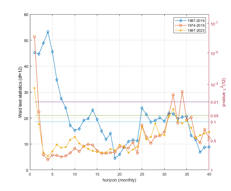
Figure 2. Multi-horizon Granger causality test from JNL to CFNAI. The X-axis displays the monthly horizon, the Y-axis displays the $p$-value. We conduct the Wald test on the first twelve GIR coefficients from JNL to CFNAI. We consider three samples: 1987-2019, 1987-2023, and 1974-2023. For robustness checks, we consider three VAR models with lag 12, 15, and 18. For each sub-sample and horizon, the presented $p$-value is the minimum one from the three VAR models. The three horizontal lines denote the significant levels of 90%, 95%, and 99%, respectively.

Figure 3: Two-stage estimates of generalized impulse responses to JNL
Refer to caption

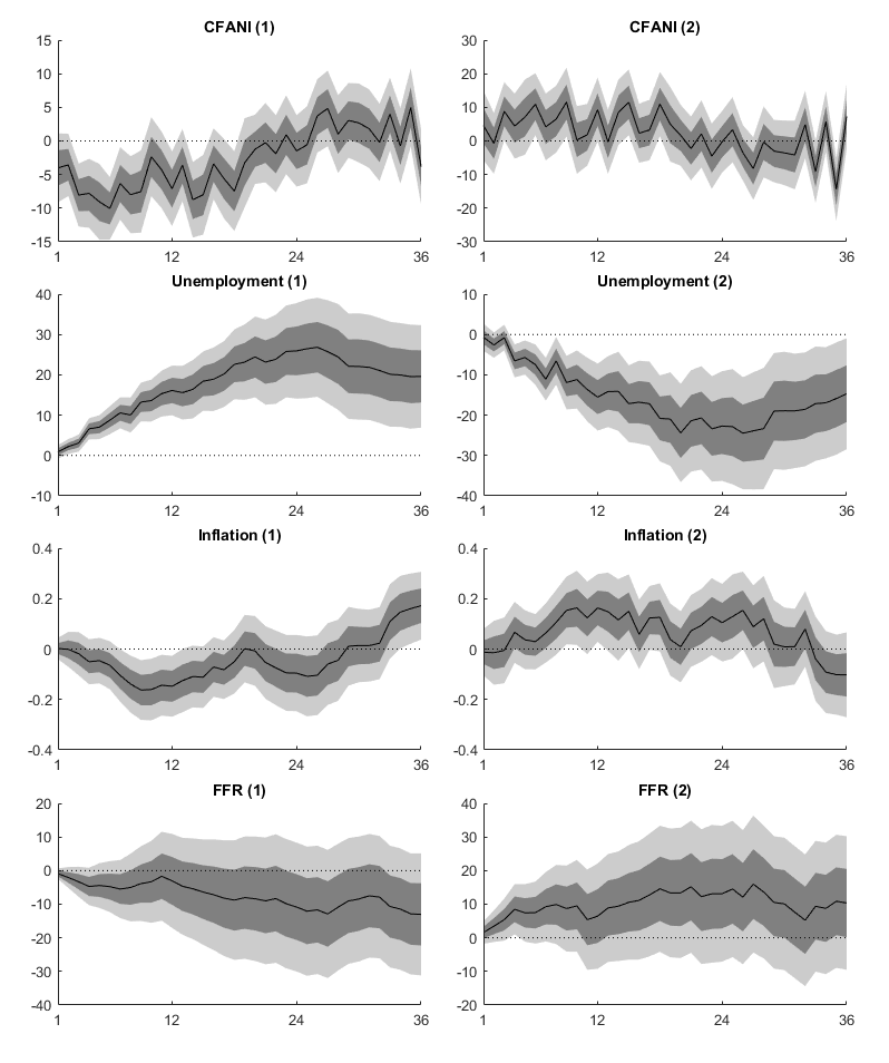
Figure 3. Two-stage estimates of GIRs to Economic uncertainty index (JNL). Note: The figure shows first two GIRs of macro-variables to economic uncertainty index (JNL). For instance, CFANI($1$) subplot displays the first GIR (the reduced-form Sims impulse response) of CFANI to JNL over 36 months; and CFANI($2$) subplot displays the second order GIR of CFANI to JNL over 36 months. The confidence interval for each estimator is built upon the asymptotic variance computed with the explicit formula of (5.42) and 68% and 95% $z$-score. The comparable GIR figures with LS projection method and recursive methods are presented in Appendix B.

Table 4:

Table 4

Two-stage estimates of generalized impulse responses

horizon Causality test two-stage estimates of twelve-lag generalized impulse responses
1 45.281* -3.999 4.584 -5.968 5.738 -4.035 0.639 4.870 -6.462 1.632 6.022 -7.614 2.496
(9.22E-06) (0.160) (0.423) (0.284) (0.269) (0.453) (0.910) (0.385) (0.198) (0.764) (0.300) (0.152) (0.619)
2 44.647* -3.565 -0.729 4.074 -2.894 -0.025 4.686 -5.894 1.182 7.435 -9.532 3.741 -0.025
(1.18E-05) (0.167) (0.885) (0.425) (0.570) (0.996) (0.380) (0.209) (0.818) (0.171) (0.061) (0.444) (0.996)
3 48.862* -8.056* 8.818 -6.188 3.975 0.443 -2.980 0.990 5.211 -7.770 4.774 -2.803 -0.731
(2.21E-06) (0.002) (0.067) (0.244) (0.487) (0.938) (0.583) (0.864) (0.387) (0.172) (0.405) (0.660) (0.913)
4 55.728* -7.790* 4.423 0.050 3.422 -6.011 3.872 3.239 -6.996 4.210 -1.891 -2.332 2.022
(1.34E-07) (0.006) (0.410) (0.993) (0.571) (0.277) (0.490) (0.585) (0.222) (0.465) (0.761) (0.721) (0.761)
5 45.654* -9.052* 7.099 0.370 -1.166 -1.963 7.439 -8.739 2.957 0.822 -3.120 0.418 4.700
(7.96E-06) (0.004) (0.254) (0.954) (0.840) (0.744) (0.240) (0.142) (0.618) (0.899) (0.647) (0.953) (0.501)
6 34.729* -10.043* 10.923* -4.996 2.004 2.445 -3.832 -0.441 1.371 -1.741 -0.337 3.848 -2.664
(0.001) (0.000) (0.033) (0.365) (0.737) (0.687) (0.501) (0.940) (0.825) (0.797) (0.962) (0.578) (0.673)
7 27.394* -6.338* 4.179 -1.441 6.309 -8.394 3.218 0.129 -3.369 1.789 2.672 -4.081 -2.652
(6.78E-03) (0.035) (0.449) (0.808) (0.302) (0.170) (0.593) (0.984) (0.623) (0.799) (0.693) (0.515) (0.652)
8 23.908* -7.998* 6.476 3.519 -4.893 -2.146 6.265 -8.511 3.942 3.728 -5.984 -1.943 6.785
(0.021) (0.012) (0.243) (0.541) (0.392) (0.706) (0.300) (0.186) (0.549) (0.562) (0.323) (0.735) (0.259)
9 17.201 -7.529* 11.565* -8.009 1.495 1.563 -4.204 1.646 3.110 -3.638 -3.805 6.487 -2.021
(0.142) (0.027) (0.042) (0.162) (0.799) (0.799) (0.506) (0.793) (0.623) (0.549) (0.519) (0.307) (0.757)
12 19.073 -7.109* 9.303 -8.101 3.384 3.520 -4.736 -4.037 8.813 -4.169 -0.005 -0.152 -0.071
(0.087) (0.021) (0.080) (0.137) (0.556) (0.564) (0.432) (0.480) (0.129) (0.493) (0.999) (0.979) (0.991)
15 19.398 -8.002* 11.491* -7.263 0.161 3.262 0.742 -4.052 0.343 1.776 -6.274 6.524 0.552
(0.079) (0.015) (0.035) (0.208) (0.978) (0.588) (0.907) (0.521) (0.957) (0.787) (0.327) (0.309) (0.936)
18 14.073 -7.460* 10.968* -4.234 0.754 -3.853 4.695 -7.847 6.297 0.614 -1.952 -1.080 0.177
(0.296) (0.024) (0.040) (0.485) (0.902) (0.527) (0.475) (0.215) (0.289) (0.919) (0.735) (0.858) (0.980)
21 10.314 -0.254 -2.242 2.473 -3.694 1.567 2.814 -3.088 0.208 -1.724 5.549 -7.879 3.465
(0.588) (0.939) (0.672) (0.675) (0.537) (0.789) (0.640) (0.589) (0.973) (0.808) (0.416) (0.228) (0.597)
24 11.192 -1.477 -0.225 4.034 -2.677 -2.833 1.510 2.949 -5.683 2.678 4.300 -10.677 13.937
(0.513) (0.619) (0.965) (0.493) (0.637) (0.638) (0.828) (0.662) (0.373) (0.670) (0.507) (0.098) (0.029)
27 21.768* 4.833 -8.216 4.579 -1.107 -2.055 -0.544 6.275 -11.425* 13.966* -19.946* 18.488* -14.127*
(0.040) (0.125) (0.115) (0.451) (0.854) (0.719) (0.927) (0.305) (0.044) (0.013) (0.001) (0.004) (0.027)
30 18.752 2.676 -3.537 -1.199 6.857 -11.838 13.102* -17.167* 15.749* -11.753 3.664 -1.679 1.953
(0.095) (0.415) (0.511) (0.844) (0.299) (0.058) (0.024) (0.003) (0.015) (0.073) (0.590) (0.810) (0.784)
33 21.628* 3.991 -9.134 10.953 -16.104* 13.919* -9.328 2.190 -0.576 0.805 -5.175 5.434 -4.660
(0.042) (0.189) (0.077) (0.051) (0.005) (0.031) (0.160) (0.735) (0.930) (0.906) (0.443) (0.394) (0.500)
36 16.861 -3.830 7.315 -8.338 1.420 1.529 -2.438 -0.442 0.549 -2.429 1.348 3.158 -1.953
(0.155) (0.221) (0.176) (0.161) (0.811) (0.799) (0.703) (0.945) (0.931) (0.730) (0.854) (0.639) (0.758)

Note - This table present two-stage estimation of twelve-lag generalized impulse response at horizon 1-9,12,15,18,21,24,27,30,33, and 36. The column of causality test displays the $p$-value of non-causality test at given horizon. The pivotal function is ${{}\mathchoice{\mbox{\boldmath$\displaystyle\mathchar 287\relax$}}{\mbox{\boldmath$\textstyle\mathchar 287\relax$}}{\mbox{\boldmath$\scriptstyle\mathchar 287\relax$}}{\mbox{\boldmath$\scriptscriptstyle\mathchar 287\relax$}}}^{2}(12)$. The numbers with sign $*$ indicate these test statistics or the coefficient estimates are statistically significant at level 95%. The comparable GIR estimates of LS projection method and recursive methods are presented in Appendix B.

Of particular interest is the finding that economic uncertainty (JNL) exhibits a causal effect on the CFNAI both in the short run (1–7 months) and the long run (approximately 2.5 years). While the short-term impact of uncertainty on economic activity is expected, its prolonged influence on the economy surpasses conventional expectations. Conversely, economic uncertainty has a sustained effect on the labor market, with JNL exerting causal influence on unemployment over a span of forty months. Surprisingly, JNL does not significantly affect the Federal Funds Rate (FFR), suggesting that the central bank may not adjust interest rates in direct response to fluctuations in economic uncertainty. Instead, the CFNAI shows causality on the FFR, which aligns with the widely held view that central banks use interest rate policy to stimulate or slow down the economy based on economic activity.

Table 4 also provides empirical evidence that statistical insignificance of impulse responses from zero does not necessarily imply zero causality over multiple horizons, and, conversely, statistically significant impulse responses from zero do not necessarily imply causality. For instance, Sims’ impulse response (the first column next to the causality test) is significant for horizons 9, 12, 15, and 18, yet none of these horizons exhibit significant multi-horizon causality tests. This discrepancy may be attributed to multicollinearity. On the other hand, at horizons 27 and 33, the causality test is statistically significant, but Sims’ impulse response is not significantly different from zero. Thus, relying solely on Sims’ impulse response for assessing multi-horizon causality could yield misleading results.

In our analysis, we specifically investigate the causality from the JNL index to CFNAI by visualizing the Wald test statistics for the null hypothesis of non-causality. Recognizing the potential sensitivity of empirical results to order selection, as highlighted by \citeasnounhamilton2004comment in the context of \citeasnounbernanke1997systematic, we conduct tests using three estimation models with lag orders of 12, 15, and 18. We report the minimum Wald test statistic across these models to ensure robustness. This approach ensures that if any Wald test statistic exceeds the critical value threshold in the plot, the results remain robust irrespective of the chosen lag order. The plot clearly illustrates that the uncertainty index does indeed exhibit causality toward economic activity, particularly around two and a half years, across all three sample periods and lag order selections.

9 Conclusion

This paper introduces a novel estimation and inference method for GIRs within a multi-horizon linear projection model. Our proposed two-stage estimation method with heteroskedasticity-robust inference complements the standard LS approach with HAC inference. The proposed covariance matrix estimation offers a robust alternative, eliminating the need for correcting serial correlation in the projection residuals. This method provides researchers with a valuable tool for applying multi-horizon linear projections in causality testing, impulse response estimation, or predictability analysis, particularly for those concerned about the efficiency of the LS projection method and the finite sample performance of HAC covariance estimates.

We derive uniform inference for two-stage estimates across the parameter space and extensively highlight the advantages of two-stage estimates over LS estimates from two key perspectives: (1) two-stage estimates generally exhibit greater efficiency than LS estimates across a wide range of parameter spaces and projection horizons, and (2) two-stage estimates can be implemented without relying on HAC standard error estimates. Instead, our explicit formula for the covariance matrix provides a positive semi-definite, heteroskedasticity-robust estimate. By allowing the projection horizon to grow with the sample size, we emphasize the crucial dependence of asymptotic normality of projection coefficient estimates on both the projection horizon and data persistence.

Our research on GIRs within a linear projection model underscores the importance of multi-horizon Granger causality in economics and finance for capturing the full dynamics of causal relationships. It also highlights the limitations of relying solely on Granger causality at horizon one or impulse response analysis when examining multi-horizon causality.

For future research, extending the finite-order VAR to an infinite-order VAR remains a promising area of interest from both theoretical and empirical perspectives. Inference for infinite-lag VAR models may require imposing restrictions on the norm of the lagged VAR coefficient matrices and carefully selecting a lag length that grows with the sample size, as discussed by \citeasnounlewis1985prediction.

Another potential extension involves exploring high-dimensional VAR models instead of finite-dimensional ones, as investigated by \citeasnounbasu2015regularized, \citeasnounadamek2023lasso, \citeasnounhecq2023granger, and others. With datasets expanding exponentially, the exploration of high-dimensionality has gained considerable attention, particularly regarding the need for robust inference on regularized coefficients. Developing a high-dimensional version of the two-stage estimation method would thus be of significant interest for future work.

References

  • [1] \harvarditem[Adamek et al.]Adamek, Smeekes and Wilms2023adamek2023lasso Adamek, R., Smeekes, S. and Wilms, I. \harvardyearleft2023\harvardyearright, ‘Lasso inference for high-dimensional time series’, Journal of Econometrics 235(2), 1114–1143.
  • [2] \harvarditem[Andrews et al.]Andrews, Cheng and Guggenberger2020andrews2020generic Andrews, D. W., Cheng, X. and Guggenberger, P. \harvardyearleft2020\harvardyearright, ‘Generic results for establishing the asymptotic size of confidence sets and tests’, Journal of Econometrics 218(2), 496–531.
  • [3] \harvarditem[Baker et al.]Baker, Bloom and Davis2016baker2016measuring Baker, S. R., Bloom, N. and Davis, S. J. \harvardyearleft2016\harvardyearright, ‘Measuring economic policy uncertainty’, The Quarterly Journal of Economics 131(4), 1593–1636.
  • [4] \harvarditemBasu and Michailidis2015basu2015regularized Basu, S. and Michailidis, G. \harvardyearleft2015\harvardyearright, ‘Regularized estimation in sparse high-dimensional time series models’, The Annals of Statistics 43(4), 1535–1567.
  • [5] \harvarditem[Benkwitz et al.]Benkwitz, Neumann and Lütekpohl2000benkwitz2000problems Benkwitz, A., Neumann, M. H. and Lütekpohl, H. \harvardyearleft2000\harvardyearright, ‘Problems related to confidence intervals for impulse responses of autoregressive processes’, Econometric Reviews 19(1), 69–103.
  • [6] \harvarditem[Bernanke et al.]Bernanke, Gertler and Watson1997bernanke1997systematic Bernanke, B. S., Gertler, M. and Watson, M. \harvardyearleft1997\harvardyearright, ‘Systematic monetary policy and the effects of oil price shocks’, Brookings papers on economic activity 1997(1), 91–157.
  • [7] \harvarditemBreitung and Brüggemann2023breitung2023projection Breitung, J. and Brüggemann, R. \harvardyearleft2023\harvardyearright, ‘Projection estimators for structural impulse responses’, Oxford Bulletin of Economics and Statistics 85(6), 1320–1340.
  • [8] \harvarditemBrockwell and Davis1991brockwell1991time Brockwell, P. J. and Davis, R. A. \harvardyearleft1991\harvardyearright, Time Series: Theory and Methods, 2 edn, Berlin: Springer Science & Business Media.
  • [9] \harvarditemCampbell and Shiller1988campbell1988dividend Campbell, J. Y. and Shiller, R. J. \harvardyearleft1988\harvardyearright, ‘The dividend-price ratio and expectations of future dividends and discount factors’, The Review of Financial Studies 1(3), 195–228.
  • [10] \harvarditemDavidson1994davidson1994stochastic Davidson, J. \harvardyearleft1994\harvardyearright, Stochastic Limit Theory: An Introduction for Econometricians, London: Oxford University Press.
  • [11] \harvarditemDiebold and Yılmaz2014diebold2014network Diebold, F. X. and Yılmaz, K. \harvardyearleft2014\harvardyearright, ‘On the network topology of variance decompositions: Measuring the connectedness of financial firms’, Journal of Econometrics 182(1), 119–134.
  • [12] \harvarditemDolado and Lütkepohl1996dolado1996making Dolado, J. J. and Lütkepohl, H. \harvardyearleft1996\harvardyearright, ‘Making Wald tests work for cointegrated VAR systems’, Econometric reviews 15(4), 369–386.
  • [13] \harvarditemDufour2003dufour2003identification Dufour, J.-M. \harvardyearleft2003\harvardyearright, ‘Identification, weak instruments, and statistical inference in econometrics’, Canadian Journal of Economics/Revue canadienne d’économique 36(4), 767–808.
  • [14] \harvarditemDufour2006dufour2006monte Dufour, J.-M. \harvardyearleft2006\harvardyearright, ‘Monte Carlo tests with nuisance parameters: A general approach to finite-sample inference and nonstandard asymptotics’, Journal of Econometrics 133(2), 443–477.
  • [15] \harvarditem[Dufour et al.]Dufour, Garcia and Taamouti2012dufour2012measuring Dufour, J.-M., Garcia, R. and Taamouti, A. \harvardyearleft2012\harvardyearright, ‘Measuring high-frequency causality between returns, realized volatility, and implied volatility’, Journal of Financial Econometrics 10(1), 124–163.
  • [16] \harvarditemDufour and Pelletier2022dufour2022practical Dufour, J.-M. and Pelletier, D. \harvardyearleft2022\harvardyearright, ‘Practical methods for modeling weak VARMA processes: Identification, estimation and specification with a macroeconomic application’, Journal of Business & Economic Statistics 40(3), 1140–1152.
  • [17] \harvarditem[Dufour et al.]Dufour, Pelletier and Renault2006dufour2006short Dufour, J.-M., Pelletier, D. and Renault, É. \harvardyearleft2006\harvardyearright, ‘Short run and long run causality in time series: inference’, Journal of Econometrics 132(2), 337–362.
  • [18] \harvarditemDufour and Renault1998dufour1998short Dufour, J.-M. and Renault, E. \harvardyearleft1998\harvardyearright, ‘Short run and long run causality in time series: theory’, Econometrica 66(5), 1099–1125.
  • [19] \harvarditem[Dufour et al.]Dufour, Renault and Zinde-Walsh2023dufour2023wald Dufour, J.-M., Renault, E. and Zinde-Walsh, V. \harvardyearleft2023\harvardyearright, ‘Wald tests when restrictions are locally singular’, CIREQ Technical Report, McGill University .
  • [20] \harvarditemDufour and Taamouti2010dufour2010short Dufour, J.-M. and Taamouti, A. \harvardyearleft2010\harvardyearright, ‘Short and long run causality measures: Theory and inference’, Journal of Econometrics 154(1), 42–58.
  • [21] \harvarditemDufour and Tessier1993dufour1993relationship Dufour, J.-M. and Tessier, D. \harvardyearleft1993\harvardyearright, ‘On the relationship between impulse response analysis, innovation accounting and Granger causality’, Economics Letters 42(4), 327–333.
  • [22] \harvarditemDufour and Valéry2015dufour2015wald Dufour, J.-M. and Valéry, P. \harvardyearleft2015\harvardyearright, ‘Wald-type tests when rank conditions fail: a smooth regularization approach’, Technical Report, McGill University and HEC Montréal .
  • [23] \harvarditemFama and French1988fama1988dividend Fama, E. F. and French, K. R. \harvardyearleft1988\harvardyearright, ‘Dividend yields and expected stock returns’, Journal of Financial Economics 22(1), 3–25.
  • [24] \harvarditem[Fernandez-Perez et al.]Fernandez-Perez, Indriawan, Tse and Xu2023fernandez2023cross Fernandez-Perez, A., Indriawan, I., Tse, Y. and Xu, Y. \harvardyearleft2023\harvardyearright, ‘Cross-asset time-series momentum: Crude oil volatility and global stock markets’, Journal of Banking & Finance 154, 106704.
  • [25] \harvarditem[Gao et al.]Gao, Hitzemann, Shaliastovich and Xu2022gao2022oil Gao, L., Hitzemann, S., Shaliastovich, I. and Xu, L. \harvardyearleft2022\harvardyearright, ‘Oil volatility risk’, Journal of Financial Economics 144(2), 456–491.
  • [26] \harvarditemGonçalves and Kilian2004gonccalves2004bootstrapping Gonçalves, S. and Kilian, L. \harvardyearleft2004\harvardyearright, ‘Bootstrapping autoregressions with conditional heteroskedasticity of unknown form’, Journal of Econometrics 123(1), 89–120.
  • [27] \harvarditemGranger1969granger1969investigating Granger, C. W. \harvardyearleft1969\harvardyearright, ‘Investigating causal relations by econometric models and cross-spectral methods’, Econometrica 37(3), 424–438.
  • [28] \harvarditemHamilton1994hamilton1994time Hamilton, J. D. \harvardyearleft1994\harvardyearright, Time Series Analysis, Princeton: Princeton University Press.
  • [29] \harvarditemHamilton and Herrera2004hamilton2004comment Hamilton, J. D. and Herrera, A. M. \harvardyearleft2004\harvardyearright, ‘Oil shocks and aggregate macroeconomic behavior: the role of monetary policy’, Journal of Money, Credit and Banking 36(2), 265–286.
  • [30] \harvarditemHannan and Rissanen1982hannan1982recursive Hannan, E. J. and Rissanen, J. \harvardyearleft1982\harvardyearright, ‘Recursive estimation of mixed autoregressive-moving average order’, Biometrika 69(1), 81–94.
  • [31] \harvarditem[Hecq et al.]Hecq, Margaritella and Smeekes2023hecq2023granger Hecq, A., Margaritella, L. and Smeekes, S. \harvardyearleft2023\harvardyearright, ‘Granger causality testing in high-dimensional VARs: a post-double-selection procedure’, Journal of Financial Econometrics 21(3), 915–958.
  • [32] \harvarditemHsiao1982hsiao1982autoregressive Hsiao, C. \harvardyearleft1982\harvardyearright, ‘Autoregressive modeling and causal ordering of economic variables’, Journal of Economic Dynamics and Control 4, 243–259.
  • [33] \harvarditemInoue and Kilian2020inoue2020uniform Inoue, A. and Kilian, L. \harvardyearleft2020\harvardyearright, ‘The uniform validity of impulse response inference in autoregressions’, Journal of Econometrics 215(2), 450–472.
  • [34] \harvarditemJordà2005jorda2005estimation Jordà, Ò. \harvardyearleft2005\harvardyearright, ‘Estimation and inference of impulse responses by local projections’, American economic review 95(1), 161–182.
  • [35] \harvarditem[Jurado et al.]Jurado, Ludvigson and Ng2015jurado2015measuring Jurado, K., Ludvigson, S. C. and Ng, S. \harvardyearleft2015\harvardyearright, ‘Measuring uncertainty’, American Economic Review 105(3), 1177–1216.
  • [36] \harvarditemKilian and Kim2011kilian2011reliable Kilian, L. and Kim, Y. J. \harvardyearleft2011\harvardyearright, ‘How reliable are local projection estimators of impulse responses?’, The Review of Economics and Statistics 93(4), 1460–1466.
  • [37] \harvarditemKilian and Lütkepohl2017kilian2017structural Kilian, L. and Lütkepohl, H. \harvardyearleft2017\harvardyearright, Structural Vector Autoregressive Analysis, Cambridge: Cambridge University Press.
  • [38] \harvarditemLewis and Reinsel1985lewis1985prediction Lewis, R. and Reinsel, G. C. \harvardyearleft1985\harvardyearright, ‘Prediction of multivariate time series by autoregressive model fitting’, Journal of Multivariate Analysis 16(3), 393–411.
  • [39] \harvarditemLütkepohl1990lutkepohl1990asymptotic Lütkepohl, H. \harvardyearleft1990\harvardyearright, ‘Asymptotic distributions of impulse response functions and forecast error variance decompositions of vector autoregressive models’, The Review of Economics and Statistics 72(1), 116–125.
  • [40] \harvarditemLütkepohl1993lutkepohl1993testing Lütkepohl, H. \harvardyearleft1993\harvardyearright, Testing for causation between two variables in higher-dimensional VAR models, in H. Schneeweiß and K. F. Zimmermann, eds, ‘Studies in Applied Econometrics’, Physica-Verlag HD, Heidelberg, pp. 75–91.
  • [41] \harvarditemLütkepohl2005lutkepohl2005new Lütkepohl, H. \harvardyearleft2005\harvardyearright, New Introduction to Multiple Time Series Analysis, Berlin: Springer Science & Business Media.
  • [42] \harvarditemLütkepohl and Burda1997lutkepohl1997modified Lütkepohl, H. and Burda, M. M. \harvardyearleft1997\harvardyearright, ‘Modified Wald tests under nonregular conditions’, Journal of Econometrics 78(2), 315–332.
  • [43] \harvarditem[Lütkepohl et al.]Lütkepohl, Staszewska-Bystrova and Winker2020lutkepohl2020constructing Lütkepohl, H., Staszewska-Bystrova, A. and Winker, P. \harvardyearleft2020\harvardyearright, ‘Constructing joint confidence bands for impulse response functions of VAR models–A review’, Econometrics and Statistics 13, 69–83.
  • [44] \harvarditemMikusheva2007mikusheva2007uniform Mikusheva, A. \harvardyearleft2007\harvardyearright, ‘Uniform inference in autoregressive models’, Econometrica 75(5), 1411–1452.
  • [45] \harvarditemMikusheva2012mikusheva2012one Mikusheva, A. \harvardyearleft2012\harvardyearright, ‘One-dimensional inference in autoregressive models with the potential presence of a unit root’, Econometrica 80(1), 173–212.
  • [46] \harvarditemMontiel Olea and Plagborg-Møller2019montiel2019simultaneous Montiel Olea, J. L. and Plagborg-Møller, M. \harvardyearleft2019\harvardyearright, ‘Simultaneous confidence bands: Theory, implementation, and an application to SVARs’, Journal of Applied Econometrics 34(1), 1–17.
  • [47] \harvarditemMontiel Olea and Plagborg-Møller2021montiel2021local Montiel Olea, J. L. and Plagborg-Møller, M. \harvardyearleft2021\harvardyearright, ‘Local projection inference is simpler and more robust than you think’, Econometrica 89(4), 1789–1823.
  • [48] \harvarditemPark and Phillips1988park1988statistical Park, J. Y. and Phillips, P. C. \harvardyearleft1988\harvardyearright, ‘Statistical inference in regressions with integrated processes: Part 1’, Econometric Theory 4(3), 468–497.
  • [49] \harvarditemPelletier2004pelletier2004problems Pelletier, D. \harvardyearleft2004\harvardyearright, ‘Problems in time series and financial econometrics: linear methods for VARMA modelling, multivariate volatility analysis, causality and value-at-risk’, Ph.D. thesis, McGill University .
  • [50] \harvarditemPhillips and Perron1988phillips1988testing Phillips, P. C. and Perron, P. \harvardyearleft1988\harvardyearright, ‘Testing for a unit root in time series regression’, Biometrika 75(2), 335–346.
  • [51] \harvarditemPlagborg-Møller and Wolf2021wolf2021same Plagborg-Møller, M. and Wolf, C. K. \harvardyearleft2021\harvardyearright, ‘Local projections and VARs estimate the same impulse responses’, Econometrica 89(2), 955–980.
  • [52] \harvarditemPope1990pope1990biases Pope, A. L. \harvardyearleft1990\harvardyearright, ‘Biases of estimators in multivariate non-gaussian autoregressions’, Journal of Time Series Analysis 11(3), 249–258.
  • [53] \harvarditemRossi and Sekhposyan2015rossi2015macroeconomic Rossi, B. and Sekhposyan, T. \harvardyearleft2015\harvardyearright, ‘Macroeconomic uncertainty indices based on nowcast and forecast error distributions’, American Economic Review 105(5), 650–655.
  • [54] \harvarditemSalamaliki and Venetis2019salamaliki2019transmission Salamaliki, P. K. and Venetis, I. A. \harvardyearleft2019\harvardyearright, ‘Transmission chains of economic uncertainty on macroeconomic activity: new empirical evidence’, Macroeconomic Dynamics 23(8), 3355–3385.
  • [55] \harvarditem[Shi et al.]Shi, Hurn and Phillips2020shi2020causal Shi, S., Hurn, S. and Phillips, P. C. \harvardyearleft2020\harvardyearright, ‘Causal change detection in possibly integrated systems: Revisiting the money–income relationship’, Journal of Financial Econometrics 18(1), 158–180.
  • [56] \harvarditemSims1980sims1980macroeconomics Sims, C. A. \harvardyearleft1980\harvardyearright, ‘Macroeconomics and reality’, Econometrica 48(1), 1–48.
  • [57] \harvarditem[Sims et al.]Sims, Stock and Watson1990sims1990inference Sims, C. A., Stock, J. H. and Watson, M. W. \harvardyearleft1990\harvardyearright, ‘Inference in linear time series models with some unit roots’, Econometrica 58(1), 113–144.
  • [58] \harvarditemStock and Watson2018stock2018identification Stock, J. H. and Watson, M. W. \harvardyearleft2018\harvardyearright, ‘Identification and estimation of dynamic causal effects in macroeconomics using external instruments’, The Economic Journal 128(610), 917–948.
  • [59] \harvarditemToda and Yamamoto1995toda1995statistical Toda, H. Y. and Yamamoto, T. \harvardyearleft1995\harvardyearright, ‘Statistical inference in vector autoregressions with possibly integrated processes’, Journal of Econometrics 66(1-2), 225–250.
  • [60] \harvarditemWiener1956wiener1956theory Wiener, N. \harvardyearleft1956\harvardyearright, ‘The theory of prediction’. in: E.F. Beckenback, ed., Modern mathematics for engineers, McGraw-Hill, New York.
  • [61] \harvarditemXu2023xu2023local Xu, K.-L. \harvardyearleft2023\harvardyearright, ‘Local projection based inference under general conditions’, Technical Report, Indiana University .
  • [62] \harvarditem[Zhang et al.]Zhang, Dufour and Galbraith2016zhang2016exchange Zhang, H. J., Dufour, J.-M. and Galbraith, J. W. \harvardyearleft2016\harvardyearright, ‘Exchange rates and commodity prices: Measuring causality at multiple horizons’, Journal of Empirical Finance 36, 100–120.
  • [63]

Appendix A Appendix: More simulation results

Table 5:

Table 5

Monte Carlo simulations: white noise process

${{}\mathchoice{\mbox{\boldmath$\displaystyle\mathchar 286\relax$}}{\mbox{\boldmath$\textstyle\mathchar 286\relax$}}{\mbox{\boldmath$\scriptstyle\mathchar 286\relax$}}{\mbox{\boldmath$\scriptscriptstyle\mathchar 286\relax$}}}_{12,1}^{(h)}$ ${{}\mathchoice{\mbox{\boldmath$\displaystyle\mathchar 286\relax$}}{\mbox{\boldmath$\textstyle\mathchar 286\relax$}}{\mbox{\boldmath$\scriptstyle\mathchar 286\relax$}}{\mbox{\boldmath$\scriptscriptstyle\mathchar 286\relax$}}}_{12,2}^{(h)}$
$h$ 1 3 6 12 24 36 1 3 6 12 24 36
value 0.000 0.000 0.000 0.000 0.000 0.000 0.000 0.000 0.000 0.000 0.000 0.000
bias of estimates
RC-VAR 0.002 1.30E-04 -1.20E-05 4.39E-07 7.22E-11 1.19E-14 0.001 -9.78E-06 -2.62E-06 4.91E-08 2.24E-11 7.43E-15
LS-Proj 0.002 0.001 -0.003 -0.001 0.002 0.002 0.001 -0.004 0.003 -0.006 -0.001 -0.003
2S(0)-Proj 0.002 0.001 -0.002 -0.001 0.002 0.002 0.001 -0.004 0.003 -0.006 -0.001 -0.003
2S(1)-Proj -0.001 0.000 -0.002 -0.002 0.001 -0.001 0.000 0.002 0.000 0.000 -0.003 -0.002
2S(2)-Proj -0.003 0.000 -0.002 0.002 -0.004 -0.001 0.000 0.001 0.009 -0.003 1.30E-04 -2.80E-04
rmse of estimates
RC-VAR 0.075 0.010 0.001 9.03E-06 1.82E-09 3.78E-13 0.075 0.007 1.94E-04 1.92E-06 5.92E-10 2.33E-13
LS-Proj 0.075 0.073 0.078 0.077 0.078 0.082 0.075 0.076 0.081 0.077 0.081 0.085
2S(0)-Proj 0.075 0.073 0.079 0.077 0.078 0.082 0.075 0.077 0.081 0.078 0.081 0.086
2S(1)-Proj 0.077 0.077 0.079 0.076 0.081 0.083 0.077 0.077 0.078 0.077 0.080 0.081
2S(2)-Proj 0.079 0.078 0.076 0.079 0.082 0.085 0.079 0.078 0.080 0.080 0.080 0.083
empirical size of tests (5% nominal size)
RC-VAR 0.054 0.001 0.000 0.000 0.000 0.000 0.047 0.001 0.000 0.000 0.000 0.000
LS-Proj 0.057 0.036 0.059 0.050 0.049 0.054 0.048 0.056 0.073 0.041 0.050 0.065
2S(0)-Proj 0.049 0.039 0.062 0.043 0.044 0.044 0.045 0.055 0.074 0.042 0.048 0.071
$\textup{2S(0)-Proj}_{b}$ 0.056 0.041 0.063 0.049 0.046 0.043 0.044 0.056 0.076 0.039 0.051 0.066
2S(1)-Proj 0.064 0.056 0.068 0.051 0.069 0.058 0.054 0.057 0.067 0.051 0.064 0.061
$\textup{2S(1)-Proj}_{b}$ 0.058 0.045 0.054 0.047 0.050 0.040 0.047 0.047 0.051 0.042 0.051 0.042
2S(2)-Proj 0.065 0.065 0.062 0.069 0.066 0.066 0.064 0.062 0.077 0.062 0.059 0.062
$\textup{2S(2)-Proj}_{b}$ 0.050 0.049 0.049 0.052 0.058 0.056 0.052 0.051 0.060 0.054 0.051 0.057
coverage ratio of nominal 95% confidence interval
RC-VAR 0.946 0.999 1.000 1.000 1.000 1.000 0.953 0.999 1.000 1.000 1.000 1.000
LS-Proj 0.943 0.964 0.941 0.950 0.951 0.946 0.952 0.944 0.927 0.959 0.950 0.935
2S(0)-Proj 0.951 0.961 0.938 0.957 0.956 0.956 0.955 0.945 0.926 0.958 0.952 0.929
$\textup{2S(0)-Proj}_{b}$ 0.944 0.959 0.937 0.951 0.954 0.957 0.956 0.944 0.924 0.961 0.949 0.934
2S(1)-Proj 0.936 0.944 0.932 0.949 0.931 0.942 0.946 0.943 0.933 0.949 0.936 0.939
$\textup{2S(1)-Proj}_{b}$ 0.942 0.955 0.946 0.953 0.950 0.960 0.953 0.953 0.949 0.958 0.949 0.958
2S(2)-Proj 0.935 0.935 0.938 0.931 0.934 0.934 0.936 0.938 0.923 0.938 0.941 0.938
$\textup{2S(2)-Proj}_{b}$ 0.950 0.951 0.951 0.948 0.942 0.944 0.948 0.949 0.940 0.946 0.949 0.943
average width of nominal 95% confidence interval
RC-VAR 0.294 0.051 0.005 2.07E-05 1.77E-09 3.87E-13 0.294 0.034 0.001 6.47E-06 7.00E-10 1.95E-13
LS-Proj 0.295 0.297 0.298 0.302 0.311 0.319 0.294 0.298 0.298 0.303 0.311 0.322
2S(0)-Proj 0.295 0.296 0.298 0.302 0.310 0.319 0.296 0.298 0.299 0.303 0.312 0.321
$\textup{2S(0)-Proj}_{b}$ 0.295 0.303 0.298 0.307 0.310 0.324 0.297 0.303 0.301 0.309 0.313 0.328
2S(1)-Proj 0.291 0.292 0.293 0.298 0.304 0.313 0.292 0.293 0.295 0.300 0.307 0.316
$\textup{2S(1)-Proj}_{b}$ 0.304 0.305 0.307 0.314 0.322 0.334 0.305 0.306 0.309 0.315 0.325 0.337
2S(2)-Proj 0.292 0.293 0.295 0.299 0.307 0.315 0.293 0.294 0.297 0.299 0.308 0.318
$\textup{2S(2)-Proj}_{b}$ 0.305 0.307 0.311 0.315 0.327 0.337 0.306 0.307 0.311 0.315 0.326 0.339

Note - The DGP follows a white noise process, $u_{t}\overset{i.i.d.}{\sim}N(0,[1,0.5;0.5,1])$.

Table 6:

Table 6

Monte Carlo simulations: I(2) process

$\displaystyle{y}_{t}=\left[\begin{array}[]{cc}1.7&-0.2\\ 0.2&1.4\end{array}\right]{y}_{t-1}+\left[\begin{array}[]{cc}-0.66&0.08\\ -0.2&-0.4\end{array}\right]{y}_{t-1}+{u}_{t}.$ (A.70)
${{}\mathchoice{\mbox{\boldmath$\displaystyle\mathchar 286\relax$}}{\mbox{\boldmath$\textstyle\mathchar 286\relax$}}{\mbox{\boldmath$\scriptstyle\mathchar 286\relax$}}{\mbox{\boldmath$\scriptscriptstyle\mathchar 286\relax$}}}_{12,1}^{(h)}$ ${{}\mathchoice{\mbox{\boldmath$\displaystyle\mathchar 286\relax$}}{\mbox{\boldmath$\textstyle\mathchar 286\relax$}}{\mbox{\boldmath$\scriptstyle\mathchar 286\relax$}}{\mbox{\boldmath$\scriptscriptstyle\mathchar 286\relax$}}}_{12,2}^{(h)}$
$h$ 1 3 6 12 24 36 1 3 6 12 24 36
value -0.200 -0.978 -2.627 -6.466 -14.445 -22.444 0.080 0.391 1.051 2.586 5.778 8.978
bias of estimates
RC-VAR -0.003 -0.018 0.015 0.492 3.033 7.087 -0.013 -0.034 -0.065 -0.264 -1.295 -2.942
LS-Proj -0.003 0.006 0.124 0.804 4.004 9.242 -0.013 -0.068 -0.224 -0.708 -2.375 -4.874
2S(2)-Proj -0.006 -0.007 0.090 0.739 3.934 9.182 -0.005 -0.012 -0.079 -0.387 -1.762 -3.966
rmse of estimates
RC-VAR 0.072 0.200 0.310 0.849 3.753 8.254 0.081 0.216 0.309 0.624 1.885 3.699
LS-Proj 0.072 0.233 0.477 1.320 5.031 10.746 0.081 0.263 0.547 1.288 3.900 7.362
2S(2)-Proj 0.084 0.211 0.393 1.132 4.713 10.365 0.149 0.254 0.352 0.750 2.380 4.776
empirical size of tests (5% nominal size)
RC-VAR 0.066 0.064 0.075 0.194 0.471 0.593 0.070 0.069 0.081 0.119 0.298 0.462
LS-Proj 0.065 0.084 0.106 0.277 0.520 0.639 0.071 0.095 0.137 0.238 0.323 0.420
2S(2)-Proj 0.078 0.061 0.080 0.224 0.489 0.636 0.086 0.064 0.090 0.172 0.327 0.417
$\textup{2S(2)-Proj}_{b}$ 0.062 0.048 0.050 0.068 0.084 0.114 0.076 0.056 0.069 0.068 0.106 0.122
coverage ratio of nominal 95% confidence interval
RC-VAR 0.934 0.936 0.925 0.806 0.529 0.407 0.930 0.931 0.919 0.881 0.702 0.538
LS-Proj 0.935 0.916 0.894 0.723 0.480 0.361 0.929 0.905 0.863 0.762 0.677 0.580
2S(2)-Proj 0.922 0.939 0.920 0.776 0.511 0.364 0.914 0.936 0.910 0.828 0.673 0.583
$\textup{2S(2)-Proj}_{b}$ 0.938 0.952 0.950 0.932 0.916 0.886 0.924 0.944 0.931 0.932 0.894 0.878
average width of nominal 95% confidence interval
RC-VAR 0.265 0.730 1.143 2.369 6.405 11.614 0.297 0.789 1.146 2.167 4.821 7.303
LS-Proj 0.266 0.831 1.614 3.362 8.823 14.233 0.298 0.917 1.749 3.632 9.703 15.937
2S(2)-Proj 0.294 0.795 1.424 2.987 8.192 14.296 0.521 0.909 1.254 2.372 5.669 10.164
$\textup{2S(2)-Proj}_{b}$ 0.307 0.859 1.593 3.694 12.819 28.260 0.537 0.954 1.382 2.772 7.611 14.729

Note - The DGP follows a VAR(2) process integrated at order two, $u_{t}\overset{i.i.d.}{\sim}N(0,[1,0.5;0.5,1])$. Two $2\times 2$ root matrices are $[0.7,-0.2;0,1]$ and $[1,0;0.2,0.4]$, whose eigenvalues are $1,0.7$ and $1,0.4$, respectively. Since the DGP contains two unit roots, only two stage results estimated with two extra lags are presented.

Appendix B Appendix: More empirical results

Figure 4: Least Squares estimates of generalized impulse responses to JNL
Refer to caption

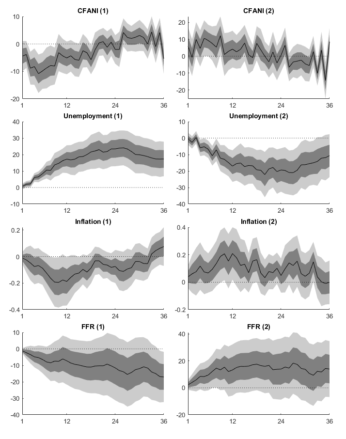
Figure 4. Projection-based Least Squares estimates of generalized impulse responses to Economic uncertainty index (JNL)

Figure 5: Recursive estimates of generalized impulse responses to JNL
Refer to caption

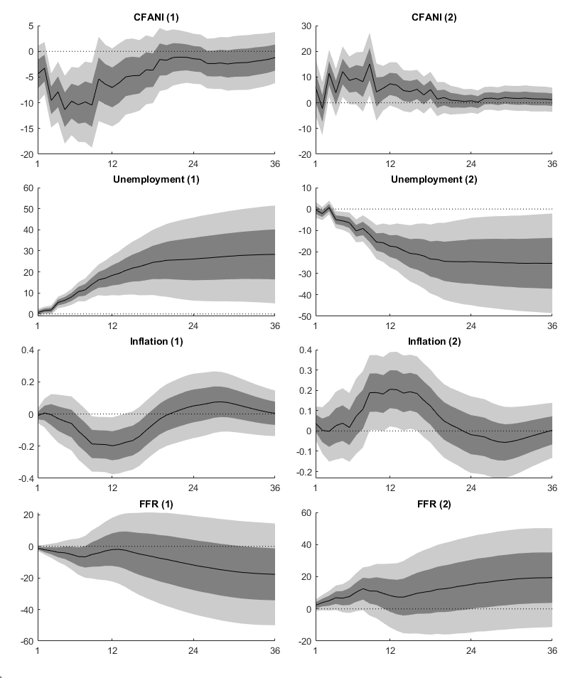
Figure 5. Recursive estimates of generalized impulse responses to Economic uncertainty index (JNL)

Table 7:

Table 7

Projection Least Squares estimates of generalized impulse responses

horizon Causality test Least Squares estimates of twelve-lag generalized impulse responses
1 28.458* -4.440 6.015 -8.599 8.689 -6.165 3.866 -0.232 -2.469 -0.420 6.176 -6.335 1.914
(0.005) (0.117) (0.284) (0.141) (0.135) (0.239) (0.413) (0.961) (0.576) (0.932) (0.275) (0.210) (0.413)
2 22.572* -3.832 -0.753 4.700 -3.740 2.033 1.681 -4.248 1.354 5.557 -8.140 4.985 -1.614
(0.032) (0.127) (0.892) (0.423) (0.456) (0.660) (0.728) (0.315) (0.784) (0.330) (0.151) (0.320) (0.491)
3 25.244* -8.820* 9.894 -7.114 6.373 -2.769 -0.911 -0.603 6.119 -9.216 8.045 -5.838 2.398
(0.014) (0.004) (0.058) (0.190) (0.217) (0.581) (0.828) (0.901) (0.308) (0.132) (0.168) (0.249) (0.359)
4 30.403* -8.240* 4.607 1.691 0.218 -2.473 1.009 4.362 -8.468 7.489 -5.289 2.080 -0.120
(0.002) (0.015) (0.400) (0.739) (0.962) (0.586) (0.849) (0.491) (0.173) (0.209) (0.343) (0.678) (0.963)
5 25.477* -10.833* 10.622* -3.119 1.891 -3.733 7.751 -10.411 7.358 -4.475 0.929 1.040 -0.286
(0.013) (0.002) (0.049) (0.546) (0.678) (0.489) (0.251) (0.107) (0.238) (0.459) (0.870) (0.847) (0.920)
6 24.932* -9.825* 9.291* -2.141 0.160 3.240 -6.370 4.403 -3.459 1.333 0.368 -0.699 0.487
(0.015) (0.003) (0.050) (0.647) (0.978) (0.633) (0.302) (0.487) (0.564) (0.818) (0.955) (0.912) (0.886)
7 25.086* -8.747* 7.527 -2.682 6.346 -8.989 6.521 -5.152 1.090 1.355 -0.530 -1.500 1.226
(0.014) (0.021) (0.144) (0.606) (0.302) (0.139) (0.313) (0.412) (0.859) (0.835) (0.931) (0.763) (0.676)
8 18.441 -7.849* 5.353 5.442 -6.392 1.819 -1.272 -0.802 0.771 2.006 -3.851 1.269 0.496
(0.103) (0.036) (0.409) (0.411) (0.297) (0.766) (0.830) (0.896) (0.906) (0.734) (0.473) (0.790) (0.862)
9 14.931 -8.043* 12.102* -8.692 4.421 -2.844 0.116 -0.365 2.409 -3.430 -0.712 2.146 -0.181
(0.245) (0.019) (0.038) (0.133) (0.502) (0.662) (0.985) (0.953) (0.679) (0.511) (0.880) (0.661) (0.952)
12 16.636 -5.090 4.170 -1.115 -2.494 6.760 -6.805 0.394 1.142 4.324 -8.061 5.103 -1.873
(0.164) (0.094) (0.453) (0.850) (0.685) (0.289) (0.257) (0.943) (0.820) (0.430) (0.167) (0.288) (0.509)
15 17.578 -5.949 7.779 -4.613 -0.790 3.534 1.338 -4.672 0.811 1.366 -6.866 10.936 -6.618
(0.129) (0.055) (0.153) (0.404) (0.866) (0.432) (0.823) (0.423) (0.878) (0.773) (0.196) (0.081) (0.081)
18 19.057 -5.751* 7.590 -0.420 -2.846 0.845 0.259 -4.743 3.627 2.909 -6.947 6.948 -5.289
(0.087) (0.033) (0.141) (0.950) (0.661) (0.872) (0.961) (0.359) (0.486) (0.554) (0.179) (0.189) (0.077)
21 26.188* 0.841 -3.358 4.070 -6.062 4.064 2.161 -5.100 0.555 -0.416 3.354 -0.911 -3.688
(0.010) (0.742) (0.480) (0.448) (0.294) (0.494) (0.691) (0.294) (0.924) (0.953) (0.599) (0.882) (0.390)
24 36.041* -2.013 0.565 5.288 -7.049 1.757 -0.671 4.526 -9.130 5.883 0.843 -0.219 -4.953
(3.19E-04) (0.450) (0.909) (0.335) (0.150) (0.740) (0.921) (0.481) (0.117) (0.276) (0.866) (0.965) (0.252)
27 22.563* 2.362 -3.452 0.670 1.055 -3.678 1.510 4.549 -9.399* 10.970* -15.232* 11.331* -6.461
(0.032) (0.369) (0.450) (0.898) (0.850) (0.512) (0.780) (0.366) (0.038) (0.025) (0.026) (0.037) (0.060)
30 26.887* 3.114 -4.569 -1.186 7.513 -12.262* 12.328* -14.308* 10.747 -7.208 0.193 -1.453 1.782
(0.008) (0.280) (0.379) (0.832) (0.204) (0.005) (0.010) (0.024) (0.095) (0.226) (0.973) (0.788) (0.531)
33 35.363* 4.380 -10.237* 10.306* -13.489* 10.865 -8.055 1.414 -0.165 1.270 -4.913 2.114 1.479
(4.10E-04) (0.128) (0.005) (0.013) (0.017) (0.083) (0.170) (0.806) (0.979) (0.839) (0.457) (0.700) (0.638)
36 25.538* -5.377 8.616* -9.267* 3.290 -1.275 0.038 -2.596 2.825 -2.501 1.987 -0.607 0.453
(0.012) (0.057) (0.038) (0.048) (0.526) (0.816) (0.994) (0.706) (0.696) (0.676) (0.748) (0.894) (0.787)

Note - This table present Least Squares estimation of twelve-lag generalized impulse response at horizon 1-9,12,15,18,21,24,27,30,33, and 36. The coefficient and covariance matrix estimation is computed through ‘hac’ command in MATLAB R2020a with setting ‘Bandwidth’=h+1. The column of ‘causality test’ displays the Wald test statistics with its $p$-value of non-causality test at given horizon. The pivotal function is ${{}\mathchoice{\mbox{\boldmath$\displaystyle\mathchar 287\relax$}}{\mbox{\boldmath$\textstyle\mathchar 287\relax$}}{\mbox{\boldmath$\scriptstyle\mathchar 287\relax$}}{\mbox{\boldmath$\scriptscriptstyle\mathchar 287\relax$}}}^{2}(12)$.

Table 8:

Table 8

Recursive VAR estimates of generalized impulse responses

horizon Causality test Recursive VAR estimates of twelve-lag generalized impulse responses
1 33.113* -4.440 6.015 -8.599 8.689 -6.165 3.866 -0.232 -2.469 -0.420 6.176 -6.335 1.914
(0.001) (0.114) (0.288) (0.147) (0.101) (0.181) (0.370) (0.957) (0.548) (0.929) (0.232) (0.169) (0.369)
2 29.642* -3.281 -2.221 6.299 -4.485 2.635 0.733 -3.447 0.323 6.502 -6.876 1.468 0.333
(0.003) (0.207) (0.672) (0.220) (0.318) (0.530) (0.859) (0.382) (0.944) (0.197) (0.126) (0.505) (0.554)
3 31.534* -9.550* 11.486* -8.191 7.037 -3.289 -0.712 -0.523 5.515 -6.453 3.385 -2.333 1.099
(0.002) (0.000) (0.014) (0.107) (0.161) (0.488) (0.872) (0.917) (0.319) (0.209) (0.320) (0.194) (0.189)
4 29.867* -7.865* 3.929 2.562 0.127 -3.488 2.358 3.033 -5.843 3.255 -1.263 -0.444 0.584
(0.003) (0.009) (0.404) (0.595) (0.978) (0.436) (0.648) (0.593) (0.262) (0.334) (0.513) (0.770) (0.487)
5 28.181* -11.340* 12.100* -4.361 2.067 -3.287 6.970 -7.806 2.809 -0.421 0.904 -2.467 1.672
(0.005) (0.001) (0.016) (0.360) (0.654) (0.535) (0.231) (0.148) (0.448) (0.855) (0.650) (0.092) (0.034)
6 25.327* -9.685* 8.702 -2.082 1.024 2.405 -3.991 0.061 0.023 1.806 -2.550 0.106 1.043
(0.013) (0.004) (0.067) (0.644) (0.849) (0.685) (0.462) (0.987) (0.993) (0.402) (0.145) (0.932) (0.175)
7 22.133* -10.394* 9.474 -2.834 6.399 -8.155 3.668 -2.277 1.754 -1.608 0.149 -0.228 0.684
(0.036) (0.005) (0.067) (0.590) (0.270) (0.129) (0.311) (0.344) (0.420) (0.382) (0.925) (0.860) (0.401)
8 19.355 -9.835* 8.194 4.026 -4.954 -0.577 1.161 -0.530 -1.351 1.879 -2.046 0.441 0.655
(0.080) (0.014) (0.167) (0.490) (0.368) (0.881) (0.628) (0.813) (0.505) (0.303) (0.217) (0.749) (0.430)
9 14.901 -10.469* 15.060* -8.241 3.382 -3.387 3.051 -3.621 2.001 -0.744 -0.204 -0.528 0.944
(0.247) (0.013) (0.016) (0.129) (0.365) (0.160) (0.142) (0.044) (0.247) (0.657) (0.890) (0.622) (0.199)
12 7.996 -7.018 7.344 -1.122 -0.829 -0.934 0.766 -1.062 1.763 -1.272 -0.463 -0.022 0.464
(0.785) (0.070) (0.087) (0.667) (0.721) (0.642) (0.639) (0.500) (0.229) (0.365) (0.739) (0.983) (0.519)
15 5.399 -4.744 4.358 -0.108 -0.549 0.285 -0.262 -0.301 -0.244 0.460 -1.340 0.445 0.305
(0.943) (0.199) (0.291) (0.959) (0.758) (0.861) (0.861) (0.831) (0.825) (0.637) (0.146) (0.528) (0.590)
18 7.140 -3.663 5.121 -2.310 1.096 -1.502 0.857 -1.171 0.497 -0.438 0.115 -0.193 0.321
(0.848) (0.262) (0.144) (0.194) (0.486) (0.256) (0.411) (0.180) (0.507) (0.504) (0.871) (0.720) (0.484)
21 4.377 -1.190 0.984 -0.358 -0.170 -0.487 -0.121 -0.077 0.149 -0.022 -0.051 -0.015 0.179
(0.976) (0.668) (0.731) (0.774) (0.858) (0.597) (0.871) (0.911) (0.811) (0.970) (0.933) (0.973) (0.639)
24 3.914 -1.448 0.762 -0.844 0.632 -0.461 0.073 -0.205 0.090 -0.025 0.341 -0.291 0.281
(0.985) (0.559) (0.748) (0.356) (0.426) (0.569) (0.910) (0.743) (0.862) (0.953) (0.484) (0.507) (0.446)
27 2.969 -2.384 1.791 -0.653 0.397 -0.567 0.171 -0.335 0.224 0.079 0.271 -0.254 0.355
(0.996) (0.343) (0.435) (0.463) (0.595) (0.434) (0.749) (0.539) (0.639) (0.846) (0.581) (0.590) (0.376)
30 3.437 -2.283 1.778 -0.540 0.241 -0.544 0.260 -0.311 0.396 -0.006 0.163 -0.132 0.357
(0.992) (0.394) (0.466) (0.475) (0.686) (0.405) (0.582) (0.542) (0.362) (0.986) (0.689) (0.738) (0.368)
33 2.742 -1.939 1.552 -0.331 0.089 -0.240 0.150 -0.154 0.368 -0.072 0.078 -0.010 0.282
(0.997) (0.472) (0.539) (0.642) (0.867) (0.704) (0.735) (0.752) (0.362) (0.811) (0.839) (0.976) (0.440)
36 2.543 -1.221 1.183 -0.143 0.000 -0.143 0.111 -0.056 0.273 -0.025 -0.044 0.096 0.192
(0.998) (0.631) (0.624) (0.823) (1.000) (0.798) (0.779) (0.899) (0.433) (0.910) (0.892) (0.723) (0.533)

Note - This table present Recursive VAR estimation of twelve-lag generalized impulse response at horizon 1-9,12,15,18,21,24,27,30,33, and 36. The coefficient and covariance matrix estimation is computed through Delta-method inference. The column of ‘causality test’ displays the Wald test statistics with its $p$-value of non-causality test at given horizon. The pivotal function is ${{}\mathchoice{\mbox{\boldmath$\displaystyle\mathchar 287\relax$}}{\mbox{\boldmath$\textstyle\mathchar 287\relax$}}{\mbox{\boldmath$\scriptstyle\mathchar 287\relax$}}{\mbox{\boldmath$\scriptscriptstyle\mathchar 287\relax$}}}^{2}(12)$.

Appendix C Appendix: Lemmas

Prior to delving into the proofs, we present a few notations and lemmas. Consider two extended transformation matrices, $\bar{G}_{1,T}$ and $\bar{G}_{2,T}$, the purpose of which is to deal with lag-augmented estimation. $\bar{G}_{1,T}$ represents a square matrix with dimensions $(p+1)K$, while $\bar{G}_{2,T}$ denotes a square matrix with dimensions $(p+2)K$,

$\displaystyle\begin{split}&\bar{G}_{1,T}:=\left[\begin{array}[]{cc}I_{K}&0\\ 0&\bar{\Upsilon}_{1}\end{array}\right]\left[\begin{array}[]{cc}I_{K}&[-P_{1},0_{K\times(p-1)K}]\\ 0_{pK\times K}&\bar{P}_{1}\end{array}\right](I_{p+1}\otimes\Pi),\\ &\bar{G}_{2,T}:=\left[\begin{array}[]{cc}I_{2K}&0\\ 0&\bar{\Upsilon}_{2}\end{array}\right]\left[\begin{array}[]{ccc}I_{K}&-(P_{1}+P_{2})&[P_{1}P_{2},0_{K\times(p-2)K}]\\ I_{K}&-(P_{1}+P_{2})&[P_{1}P_{2},0_{K\times(p-2)K}]\\ 0_{pK\times K}&0_{pK\times K}&\bar{P}_{2}\end{array}\right](I_{p+2}\otimes\Pi).\end{split}$ (C.71)

The matrices $\bar{G}_{1,T}$ and $\bar{G}_{2,T}$ are composed of three distinct components, each serving a crucial role. First, the matrix $\Pi$ is to eliminate potential cointegration within the vector of observables $y_{t}$. Second, the matrix containing $P_{1},P_{2}$ is to derive Dickey-Fuller type regressors. Finally, the component involving $\bar{\Upsilon}_{i}$ represents a probability scaling matrix, accommodating varying convergence speeds for potential non-stationary processes.

Then, we introduce notations for rotated and differenced $y_{t}$ and $x_{t}$:

$\displaystyle\tilde{y}_{t}=\Pi y_{t}$ (C.72)
$\displaystyle\Delta_{10}\tilde{y}_{t}=(I_{K}-P_{1}L)\tilde{y}_{t}$ (C.73)
$\displaystyle\Delta_{21}\tilde{y}_{t}=(I_{K}-P_{2}L)\tilde{y}_{t}$ (C.74)
$\displaystyle\Delta_{20}\tilde{y}_{t}=(I_{K}-P_{1}L)(I_{K}-P_{2}L)\tilde{y}_{t}$ (C.75)

and

$\displaystyle\tilde{x}_{t}=(I_{p}\otimes\Pi)x_{t}$ (C.76)
$\displaystyle\Delta_{10}\tilde{x}_{t}=(I_{pK}-I_{p}\otimes P_{1}L)\tilde{x}_{t}$ (C.77)
$\displaystyle\Delta_{21}\tilde{x}_{t}=(I_{pK}-I_{p}\otimes P_{2}L)\tilde{x}_{t}$ (C.78)
$\displaystyle\Delta_{20}\tilde{x}_{t}=(I_{pK}-I_{p}\otimes P_{1}L)(I_{pK}-I_{p}\otimes P_{2}L)\tilde{x}_{t}.$ (C.79)
Lemma C.1 (Boundedness of impulse responses)

Let the autoregressive coefficients be in the parameter space $\mathcal{B}({{}\mathchoice{\mbox{\boldmath$\displaystyle\mathchar 270\relax$}}{\mbox{\boldmath$\textstyle\mathchar 270\relax$}}{\mbox{\boldmath$\scriptstyle\mathchar 270\relax$}}{\mbox{\boldmath$\scriptscriptstyle\mathchar 270\relax$}}},c,{{}\mathchoice{\mbox{\boldmath$\displaystyle\mathchar 271\relax$}}{\mbox{\boldmath$\textstyle\mathchar 271\relax$}}{\mbox{\boldmath$\scriptstyle\mathchar 271\relax$}}{\mbox{\boldmath$\scriptscriptstyle\mathchar 271\relax$}}})$. Let $c=(c_{0},c_{1})$, $c_{0},c_{1}>0$, ${{}\mathchoice{\mbox{\boldmath$\displaystyle\mathchar 271\relax$}}{\mbox{\boldmath$\textstyle\mathchar 271\relax$}}{\mbox{\boldmath$\scriptstyle\mathchar 271\relax$}}{\mbox{\boldmath$\scriptscriptstyle\mathchar 271\relax$}}}\in(0,1)$.

  1. (i)

    If ${{}\mathchoice{\mbox{\boldmath$\displaystyle\mathchar 270\relax$}}{\mbox{\boldmath$\textstyle\mathchar 270\relax$}}{\mbox{\boldmath$\scriptstyle\mathchar 270\relax$}}{\mbox{\boldmath$\scriptscriptstyle\mathchar 270\relax$}}}=0$, then

    $\displaystyle\sum_{i=0}^{\infty}\|\Psi_{i}\|=O_{p}(1),$ (C.80)
    $\displaystyle\sum_{i=0}^{\infty}\|\Psi_{i}\|^{2}=O_{p}(1).$ (C.81)
  2. (ii)

    If ${{}\mathchoice{\mbox{\boldmath$\displaystyle\mathchar 270\relax$}}{\mbox{\boldmath$\textstyle\mathchar 270\relax$}}{\mbox{\boldmath$\scriptstyle\mathchar 270\relax$}}{\mbox{\boldmath$\scriptscriptstyle\mathchar 270\relax$}}}=1$, then

    $\displaystyle\sum_{i=0}^{h-1}\|\Psi_{i}\|=O_{p}(h),$ (C.82)
    $\displaystyle\sum_{i=0}^{h-1}\|\Psi_{i}\|^{2}=O_{p}(h).$ (C.83)
  3. (iii)

    If ${{}\mathchoice{\mbox{\boldmath$\displaystyle\mathchar 270\relax$}}{\mbox{\boldmath$\textstyle\mathchar 270\relax$}}{\mbox{\boldmath$\scriptstyle\mathchar 270\relax$}}{\mbox{\boldmath$\scriptscriptstyle\mathchar 270\relax$}}}=2$, then

    $\displaystyle\sum_{i=0}^{h-1}\|\Psi_{i}\|=O_{p}(h^{2}),$ (C.84)
    $\displaystyle\sum_{i=0}^{h-1}\|\Psi_{i}\|^{2}=O_{p}(h^{3}).$ (C.85)

See the proof in Subsection D.7.

Lemma C.2 (Boundedness of the LRV)

Suppose Assumption 4.1 and 4.2(i) hold. Let $w\in\mathbb{R}^{pK}$, $\|w\|=1$, $\underline{c}_{{{}\mathchoice{\mbox{\boldmath$\displaystyle\mathchar 280\relax$}}{\mbox{\boldmath$\textstyle\mathchar 280\relax$}}{\mbox{\boldmath$\scriptstyle\mathchar 280\relax$}}{\mbox{\boldmath$\scriptscriptstyle\mathchar 280\relax$}}}},\overline{c}_{{{}\mathchoice{\mbox{\boldmath$\displaystyle\mathchar 280\relax$}}{\mbox{\boldmath$\textstyle\mathchar 280\relax$}}{\mbox{\boldmath$\scriptstyle\mathchar 280\relax$}}{\mbox{\boldmath$\scriptscriptstyle\mathchar 280\relax$}}}}$ are positive constant, and $0<\underline{c}_{{{}\mathchoice{\mbox{\boldmath$\displaystyle\mathchar 280\relax$}}{\mbox{\boldmath$\textstyle\mathchar 280\relax$}}{\mbox{\boldmath$\scriptstyle\mathchar 280\relax$}}{\mbox{\boldmath$\scriptscriptstyle\mathchar 280\relax$}}}}\leq\overline{c}_{{{}\mathchoice{\mbox{\boldmath$\displaystyle\mathchar 280\relax$}}{\mbox{\boldmath$\textstyle\mathchar 280\relax$}}{\mbox{\boldmath$\scriptstyle\mathchar 280\relax$}}{\mbox{\boldmath$\scriptscriptstyle\mathchar 280\relax$}}}}<\infty$. Then, the long run variance $\Omega_{s,h}$ defined in (4.32) is bounded:

$\displaystyle 0<\underline{c}_{{{}\mathchoice{\mbox{\boldmath$\displaystyle\mathchar 280\relax$}}{\mbox{\boldmath$\textstyle\mathchar 280\relax$}}{\mbox{\boldmath$\scriptstyle\mathchar 280\relax$}}{\mbox{\boldmath$\scriptscriptstyle\mathchar 280\relax$}}}}\sum_{j=1}^{h+p-1}{{}\mathchoice{\mbox{\boldmath$\displaystyle\mathchar 288\relax$}}{\mbox{\boldmath$\textstyle\mathchar 288\relax$}}{\mbox{\boldmath$\scriptstyle\mathchar 288\relax$}}{\mbox{\boldmath$\scriptscriptstyle\mathchar 288\relax$}}}_{w,j}\leq w^{\prime}\Omega_{s,h}w\leq\overline{c}_{{{}\mathchoice{\mbox{\boldmath$\displaystyle\mathchar 280\relax$}}{\mbox{\boldmath$\textstyle\mathchar 280\relax$}}{\mbox{\boldmath$\scriptstyle\mathchar 280\relax$}}{\mbox{\boldmath$\scriptscriptstyle\mathchar 280\relax$}}}}\sum_{j=1}^{h+p-1}{{}\mathchoice{\mbox{\boldmath$\displaystyle\mathchar 288\relax$}}{\mbox{\boldmath$\textstyle\mathchar 288\relax$}}{\mbox{\boldmath$\scriptstyle\mathchar 288\relax$}}{\mbox{\boldmath$\scriptscriptstyle\mathchar 288\relax$}}}_{w,j},$ (C.86)

where ${{}\mathchoice{\mbox{\boldmath$\displaystyle\mathchar 288\relax$}}{\mbox{\boldmath$\textstyle\mathchar 288\relax$}}{\mbox{\boldmath$\scriptstyle\mathchar 288\relax$}}{\mbox{\boldmath$\scriptscriptstyle\mathchar 288\relax$}}}_{w,j}=\|\sum_{i=\max(1,j-h+1)}^{\min(p,j)}w_{i}\Psi_{1\bullet,h-j+i-1}\|^{2}$, $w_{i}$ is the $K$-dimensional sub-vector of $w$, $w=(w_{1}^{\prime},w_{2}^{\prime},\cdots,w_{p}^{\prime})^{\prime}$.

See the proof in Subsection D.8.

Lemma C.3 (Variance of variance estimates of regression score function)

Let the conditions of Proposition (4.3) hold, then

$\displaystyle\text{Var}\left((\bar{T}-p+1)^{-1}\sum_{t=p}^{\bar{T}}(w^{\prime}s_{t,h}^{*})^{2}/w^{\prime}\Omega_{s,h}w\right)\xrightarrow{p}0.$ (C.87)

See the proof in Subsection D.9.

Lemma C.4 (Bounded fourth moments of regression score function)

Suppose Assumption 4.1 and 4.2(i) hold. Then

$\displaystyle\mathbb{E}[(w^{\prime}s_{t,h}^{*})^{4}/(w^{\prime}\Omega_{s,h}w)^{2}]<c_{0}<\infty$ (C.88)

where $w\in\mathbb{R}^{pK}$, $\|w\|=1$, for some constant $c_{0}$ almost surely.

See the proof in Subsection D.10.

Lemma C.5 (Boundedness of the second moments)

Suppose Assumption 4.1 and 4.2 hold. Then

$\displaystyle\lim_{T\rightarrow\infty}T^{-1}\sum_{t=1}^{T}u_{t}u_{t}^{\prime}\xrightarrow{p}\Sigma_{u}.$ (C.89)

Moreover, let the autoregressive coefficients be in the parameter space $\mathcal{B}({{}\mathchoice{\mbox{\boldmath$\displaystyle\mathchar 270\relax$}}{\mbox{\boldmath$\textstyle\mathchar 270\relax$}}{\mbox{\boldmath$\scriptstyle\mathchar 270\relax$}}{\mbox{\boldmath$\scriptscriptstyle\mathchar 270\relax$}}},c,{{}\mathchoice{\mbox{\boldmath$\displaystyle\mathchar 271\relax$}}{\mbox{\boldmath$\textstyle\mathchar 271\relax$}}{\mbox{\boldmath$\scriptstyle\mathchar 271\relax$}}{\mbox{\boldmath$\scriptscriptstyle\mathchar 271\relax$}}})$. Let $c=(c_{0},c_{1})$, $c_{0},c_{1}>0$, ${{}\mathchoice{\mbox{\boldmath$\displaystyle\mathchar 271\relax$}}{\mbox{\boldmath$\textstyle\mathchar 271\relax$}}{\mbox{\boldmath$\scriptstyle\mathchar 271\relax$}}{\mbox{\boldmath$\scriptscriptstyle\mathchar 271\relax$}}}\in(0,1)$.

  1. (i)

    If ${{}\mathchoice{\mbox{\boldmath$\displaystyle\mathchar 270\relax$}}{\mbox{\boldmath$\textstyle\mathchar 270\relax$}}{\mbox{\boldmath$\scriptstyle\mathchar 270\relax$}}{\mbox{\boldmath$\scriptscriptstyle\mathchar 270\relax$}}}=0$ and $0<h/T\leq{{}\mathchoice{\mbox{\boldmath$\displaystyle\mathchar 267\relax$}}{\mbox{\boldmath$\textstyle\mathchar 267\relax$}}{\mbox{\boldmath$\scriptstyle\mathchar 267\relax$}}{\mbox{\boldmath$\scriptscriptstyle\mathchar 267\relax$}}}$ for ${{}\mathchoice{\mbox{\boldmath$\displaystyle\mathchar 267\relax$}}{\mbox{\boldmath$\textstyle\mathchar 267\relax$}}{\mbox{\boldmath$\scriptstyle\mathchar 267\relax$}}{\mbox{\boldmath$\scriptscriptstyle\mathchar 267\relax$}}}\in[0,1)$, then

    $\displaystyle\lim_{T\rightarrow\infty}T^{-1}\sum_{t=p}^{T}z_{t}x_{t}^{\prime}\xrightarrow{p}\mathbb{E}[z_{t}x_{t}^{\prime}],$ (C.90)
    $\displaystyle\lim_{T\rightarrow\infty}\|T^{-1}\sum_{t=1}^{T}x_{t}x_{t}^{\prime}\|=O_{p}(1),$ (C.91)
    $\displaystyle\lim_{T\rightarrow\infty}\|T^{-1/2}\sum_{t=1}^{T}x_{t}u_{t+k}^{\prime}\|=O_{p}(1),$ (C.92)
    $\displaystyle\lim_{T\rightarrow\infty}\|\bar{T}^{-1/2}\sum_{t=p}^{T-h}x_{t}e_{t+k,h}\|=O_{p}(1),$ (C.93)
  2. (ii)

    If ${{}\mathchoice{\mbox{\boldmath$\displaystyle\mathchar 270\relax$}}{\mbox{\boldmath$\textstyle\mathchar 270\relax$}}{\mbox{\boldmath$\scriptstyle\mathchar 270\relax$}}{\mbox{\boldmath$\scriptscriptstyle\mathchar 270\relax$}}}=1$ and $\frac{h}{T}\max(1,\frac{h}{w^{\prime}\Omega_{{{}\mathchoice{\mbox{\boldmath$\displaystyle\mathchar 268\relax$}}{\mbox{\boldmath$\textstyle\mathchar 268\relax$}}{\mbox{\boldmath$\scriptstyle\mathchar 268\relax$}}{\mbox{\boldmath$\scriptscriptstyle\mathchar 268\relax$}}},h}w})\xrightarrow{p}0$, then

    $\displaystyle\lim_{T\rightarrow\infty}T^{-1}\sum_{t=p}^{T}z_{t}\Delta_{10}\tilde{x}_{t}^{\prime}\xrightarrow{p}\mathbb{E}[z_{t}\Delta_{10}\tilde{x}_{t}^{\prime}],$ (C.94)
    $\displaystyle\lim_{T\rightarrow\infty}\|T^{-1}\sum_{t=1}^{T}G_{1,T}x_{t}x_{t}^{\prime}G_{1,T}^{\prime}\|=O_{p}(1).$ (C.95)
    $\displaystyle\lim_{T\rightarrow\infty}\|T^{-1/2}\sum_{t=1}^{T}G_{1,T}x_{t}u_{t+k}^{\prime}\|=O_{p}(1),$ (C.96)
    $\displaystyle\lim_{T\rightarrow\infty}\|T^{-1/2}\sum_{t=1}^{T}\Upsilon_{1}\tilde{y}_{t}u_{t+k}\|=O_{p}(1),$ (C.97)
    $\displaystyle\lim_{T\rightarrow\infty}\|\bar{T}^{-1/2}\sum_{t=p}^{T-h}G_{1,T}x_{t}e_{t+k,h}\|=O_{p}(h),$ (C.98)
  3. (iii)

    If ${{}\mathchoice{\mbox{\boldmath$\displaystyle\mathchar 270\relax$}}{\mbox{\boldmath$\textstyle\mathchar 270\relax$}}{\mbox{\boldmath$\scriptstyle\mathchar 270\relax$}}{\mbox{\boldmath$\scriptscriptstyle\mathchar 270\relax$}}}=2$ and $\frac{h^{3}}{T}\max(1,\frac{h}{w^{\prime}\Omega_{{{}\mathchoice{\mbox{\boldmath$\displaystyle\mathchar 268\relax$}}{\mbox{\boldmath$\textstyle\mathchar 268\relax$}}{\mbox{\boldmath$\scriptstyle\mathchar 268\relax$}}{\mbox{\boldmath$\scriptscriptstyle\mathchar 268\relax$}}},h}w})\xrightarrow{p}0$, then

    $\displaystyle\lim_{T\rightarrow\infty}T^{-1}\sum_{t=p}^{T}z_{t}\Delta_{20}\tilde{x}_{t}^{\prime}\xrightarrow{p}\mathbb{E}[z_{t}\Delta_{20}\tilde{x}_{t}^{\prime}],$ (C.99)
    $\displaystyle\lim_{T\rightarrow\infty}\|T^{-1}\sum_{t=1}^{T}G_{2,T}x_{t}x_{t}^{\prime}G_{2,T}^{\prime}\|=O_{p}(1),$ (C.100)
    $\displaystyle\lim_{T\rightarrow\infty}\|T^{-1/2}\sum_{t=1}^{T}G_{2,T}x_{t}u_{t+k}^{\prime}\|=O_{p}(1),$ (C.101)
    $\displaystyle\lim_{T\rightarrow\infty}\|T^{-1/2}\sum_{t=1}^{T}u_{t+k}(\tilde{y}_{t}^{\prime}\Upsilon_{2},\Delta_{21}\tilde{y}_{t}^{\prime}\Upsilon_{1})\|=O_{p}(1),$ (C.102)
    $\displaystyle\lim_{T\rightarrow\infty}\|\bar{T}^{-1/2}\sum_{t=p}^{T-h}G_{2,T}x_{t}e_{t+k,h}\|=O_{p}(h^{2}).$ (C.103)

for any non-negative integer $k$.

See the proof in Subsection D.11.

Lemma C.6 (Asymptotically negligible estimation errors)

Suppose Assumption 4.1, 4.2, and 5.1 hold. Let the autoregressive coefficients be in the parameter space $\mathcal{B}({{}\mathchoice{\mbox{\boldmath$\displaystyle\mathchar 270\relax$}}{\mbox{\boldmath$\textstyle\mathchar 270\relax$}}{\mbox{\boldmath$\scriptstyle\mathchar 270\relax$}}{\mbox{\boldmath$\scriptscriptstyle\mathchar 270\relax$}}},c,{{}\mathchoice{\mbox{\boldmath$\displaystyle\mathchar 271\relax$}}{\mbox{\boldmath$\textstyle\mathchar 271\relax$}}{\mbox{\boldmath$\scriptstyle\mathchar 271\relax$}}{\mbox{\boldmath$\scriptscriptstyle\mathchar 271\relax$}}})$. Let $c=(c_{0},c_{1})$, $c_{0},c_{1}>0$, ${{}\mathchoice{\mbox{\boldmath$\displaystyle\mathchar 271\relax$}}{\mbox{\boldmath$\textstyle\mathchar 271\relax$}}{\mbox{\boldmath$\scriptstyle\mathchar 271\relax$}}{\mbox{\boldmath$\scriptscriptstyle\mathchar 271\relax$}}}\in(0,1)$, and $w\in\mathbb{R}^{pK}$, and $\|w\|=1$. If one of the following conditions hold,

  1. (i)

    ${{}\mathchoice{\mbox{\boldmath$\displaystyle\mathchar 270\relax$}}{\mbox{\boldmath$\textstyle\mathchar 270\relax$}}{\mbox{\boldmath$\scriptstyle\mathchar 270\relax$}}{\mbox{\boldmath$\scriptscriptstyle\mathchar 270\relax$}}}=0$ and $0<h/T\leq{{}\mathchoice{\mbox{\boldmath$\displaystyle\mathchar 267\relax$}}{\mbox{\boldmath$\textstyle\mathchar 267\relax$}}{\mbox{\boldmath$\scriptstyle\mathchar 267\relax$}}{\mbox{\boldmath$\scriptscriptstyle\mathchar 267\relax$}}}$ for ${{}\mathchoice{\mbox{\boldmath$\displaystyle\mathchar 267\relax$}}{\mbox{\boldmath$\textstyle\mathchar 267\relax$}}{\mbox{\boldmath$\scriptstyle\mathchar 267\relax$}}{\mbox{\boldmath$\scriptscriptstyle\mathchar 267\relax$}}}\in[0,1)$,

  2. (ii)

    ${{}\mathchoice{\mbox{\boldmath$\displaystyle\mathchar 270\relax$}}{\mbox{\boldmath$\textstyle\mathchar 270\relax$}}{\mbox{\boldmath$\scriptstyle\mathchar 270\relax$}}{\mbox{\boldmath$\scriptscriptstyle\mathchar 270\relax$}}}=1$ and $\frac{h}{T}\max(1,\frac{h}{w^{\prime}\Omega_{{{}\mathchoice{\mbox{\boldmath$\displaystyle\mathchar 268\relax$}}{\mbox{\boldmath$\textstyle\mathchar 268\relax$}}{\mbox{\boldmath$\scriptstyle\mathchar 268\relax$}}{\mbox{\boldmath$\scriptscriptstyle\mathchar 268\relax$}}},h}w})\xrightarrow{p}0$,

  3. (iii)

    ${{}\mathchoice{\mbox{\boldmath$\displaystyle\mathchar 270\relax$}}{\mbox{\boldmath$\textstyle\mathchar 270\relax$}}{\mbox{\boldmath$\scriptstyle\mathchar 270\relax$}}{\mbox{\boldmath$\scriptscriptstyle\mathchar 270\relax$}}}=2$ and $\frac{h^{3}}{T}\max(1,\frac{h}{w^{\prime}\Omega_{{{}\mathchoice{\mbox{\boldmath$\displaystyle\mathchar 268\relax$}}{\mbox{\boldmath$\textstyle\mathchar 268\relax$}}{\mbox{\boldmath$\scriptstyle\mathchar 268\relax$}}{\mbox{\boldmath$\scriptscriptstyle\mathchar 268\relax$}}},h}w})\xrightarrow{p}0$,

then

$\displaystyle\lim_{T\rightarrow\infty}\|\bar{T}^{-1/2}\sum_{t=p}^{T-h}(\hat{z}_{t}-z_{t})x_{t-k}^{\prime}G_{{{}\mathchoice{\mbox{\boldmath$\displaystyle\mathchar 270\relax$}}{\mbox{\boldmath$\textstyle\mathchar 270\relax$}}{\mbox{\boldmath$\scriptstyle\mathchar 270\relax$}}{\mbox{\boldmath$\scriptscriptstyle\mathchar 270\relax$}}},T}^{\prime}\|=O_{p}(1),$ (C.104)
$\displaystyle\lim_{T\rightarrow\infty}\left\|\frac{1}{\left(\bar{T}w^{\prime}\Omega_{{{}\mathchoice{\mbox{\boldmath$\displaystyle\mathchar 268\relax$}}{\mbox{\boldmath$\textstyle\mathchar 268\relax$}}{\mbox{\boldmath$\scriptstyle\mathchar 268\relax$}}{\mbox{\boldmath$\scriptscriptstyle\mathchar 268\relax$}}},h}w\right)^{1/2}}\sum_{t=p}^{T-h}(\hat{z}_{t}-z_{t})e_{t,h}\right\|\xrightarrow{p}0,$ (C.105)

for finite non-negative integer $k$.

See the proof in Subsection D.12.

Lemma C.7 (Boundedness of the fourth moment)

Suppose Assumption 4.1, 4.2, and 5.1 hold. Let the autoregressive coefficients be in the parameter space $\mathcal{B}({{}\mathchoice{\mbox{\boldmath$\displaystyle\mathchar 270\relax$}}{\mbox{\boldmath$\textstyle\mathchar 270\relax$}}{\mbox{\boldmath$\scriptstyle\mathchar 270\relax$}}{\mbox{\boldmath$\scriptscriptstyle\mathchar 270\relax$}}},c,{{}\mathchoice{\mbox{\boldmath$\displaystyle\mathchar 271\relax$}}{\mbox{\boldmath$\textstyle\mathchar 271\relax$}}{\mbox{\boldmath$\scriptstyle\mathchar 271\relax$}}{\mbox{\boldmath$\scriptscriptstyle\mathchar 271\relax$}}})$. Let $c=(c_{0},c_{1})$, $c_{0},c_{1}>0$, ${{}\mathchoice{\mbox{\boldmath$\displaystyle\mathchar 271\relax$}}{\mbox{\boldmath$\textstyle\mathchar 271\relax$}}{\mbox{\boldmath$\scriptstyle\mathchar 271\relax$}}{\mbox{\boldmath$\scriptscriptstyle\mathchar 271\relax$}}}\in(0,1)$, and $w\in\mathbb{R}^{pK}$, and $\|w\|=1$. Denote $\tilde{y}_{t}=\Pi y_{t}$.

  1. (i)

    If ${{}\mathchoice{\mbox{\boldmath$\displaystyle\mathchar 270\relax$}}{\mbox{\boldmath$\textstyle\mathchar 270\relax$}}{\mbox{\boldmath$\scriptstyle\mathchar 270\relax$}}{\mbox{\boldmath$\scriptscriptstyle\mathchar 270\relax$}}}=0$, then

    $\displaystyle\max_{1\leq t\leq T}\mathbb{E}[\|\tilde{y}_{t}\|^{4}]=O_{p}(1).$ (C.106)
  2. (ii)

    If ${{}\mathchoice{\mbox{\boldmath$\displaystyle\mathchar 270\relax$}}{\mbox{\boldmath$\textstyle\mathchar 270\relax$}}{\mbox{\boldmath$\scriptstyle\mathchar 270\relax$}}{\mbox{\boldmath$\scriptscriptstyle\mathchar 270\relax$}}}=1$, then

    $\displaystyle\max_{1\leq t\leq T}\mathbb{E}[\|\Upsilon_{1}\tilde{y}_{t}\|^{4}]=O_{p}(1).$ (C.107)
  3. (iii)

    If ${{}\mathchoice{\mbox{\boldmath$\displaystyle\mathchar 270\relax$}}{\mbox{\boldmath$\textstyle\mathchar 270\relax$}}{\mbox{\boldmath$\scriptstyle\mathchar 270\relax$}}{\mbox{\boldmath$\scriptscriptstyle\mathchar 270\relax$}}}=2$, then

    $\displaystyle\max_{1\leq t\leq T}\mathbb{E}[\|\Upsilon_{2}\tilde{y}_{t}\|^{4}]=O_{p}(1).$ (C.108)

See the proof in Subsection D.13.

Appendix D Appendix: Proofs

D.1 Lemma 4.1 (LRV matrix)

Proof.

First we show $\text{LRV}(s_{t,h}^{*})=\Omega_{s,h}$. Recall the explicit form of $s_{t,h}$ in (4.30). We partition $s_{t,h}$ as $s_{t,h}=(s_{1,t,h}^{\prime},s_{2,t,h}^{\prime},\cdots,s_{p,t,h}^{\prime})^{\prime}$ where $s_{i,t,h}=u_{t+i-1}e_{t,h}$. Thus, given the explicit form of $s_{t,h}^{*}$ in (4.33), $s_{t,h}^{*}=(s_{1,t,h}^{\prime},s_{2,t+1,h}^{\prime},\cdots,s_{p,t+p-1,h}^{\prime})^{\prime}$. As $\Omega_{s,h}$ is the LRV of $s_{t,h}$, we partition $\Omega_{s,h}$ into $p\times p$ block matrices of dimension $K$,

$\displaystyle\Omega_{s,h}=\left[\Omega_{s,h}^{(ij)}\right]_{i,j=1,2,\cdots,p},$ (D.109)

where $\Omega_{s,h}^{(ij)}$ is a $K$-dimensional square matrix, $\Omega_{s,h}^{(ij)}=\sum_{k=-\infty}^{\infty}\mathbb{E}[s_{i,t,h}s_{j,t+k,h}^{\prime}]$. Under Assumption (4.1), $\Omega_{s,h}^{(ij)}=\sum_{k=-h+1}^{h-1}\mathbb{E}[s_{i,t,h}s_{j,t+k,h}^{\prime}]$, as $\mathbb{E}[s_{i,t,h}s_{j,t+k,h}^{\prime}]=0$ for all $|k|\geq h$.

Since $s_{t,h}^{*}=(s_{1,t,h}^{\prime},s_{2,t+1,h}^{\prime},\cdots,s_{p,t+p-1,h}^{\prime})^{\prime}$, to prove $\text{LRV}(s_{t,h}^{*})=\Omega_{s,h}$, it is equivalent to show $\sum_{k=-\infty}^{\infty}\mathbb{E}[s_{i,t+i-1,h}s_{j,t+k+j-1,h}^{\prime}]=\Omega_{s,h}^{(ij)}$.

$\displaystyle\begin{split}\sum_{k=-\infty}^{\infty}\mathbb{E}[s_{i,t+i-1,h}s_{j,t+k+j-1,h}^{\prime}]&=\sum_{k=-\infty}^{\infty}\mathbb{E}[s_{i,t,h}s_{j,t+k+j-i,h}^{\prime}]\\ &\quad(\text{ because of covariance stationary of $s_{t,h}$})\\ &=\sum_{k=-h+1+i-j}^{h-1+i-j}\mathbb{E}[s_{i,t,h}s_{j,t+k+j-i,h}^{\prime}]\\ &\quad(\text{ since $\mathbb{E}[s_{i,t,h}s_{j,t+k,h}^{\prime}]=0$ for all $|k|\geq h$})\\ &=\sum_{k=-h+1}^{h-1}\mathbb{E}[s_{i,t,h}s_{j,t+k,h}^{\prime}]=\Omega_{s,h}^{(ij)}\\ &\quad(\text{ replacing $k+j-i$ by $k$})\end{split}$ (D.110)

Thus, we have completed the proof of $\text{LRV}(s_{t,h}^{*})=\Omega_{s,h}$.

Next, we show $\text{LRV}(s_{t,h}^{*})=\text{Var}(s_{t,h}^{*})$. To prove the identity between LRV and variance, it is equivalent to show the serial uncorrelation of $s_{t,h}^{*}$. Without loss of generality, suppose $k>0$

𝔼[st+k,hst,h]=𝔼[𝔼[st+k,hst,h{u𝝉}𝝉>t]] (Law of Iterated Expectations)=𝔼[st+k,h𝔼[st,h{u𝝉}𝝉>t]] (Since st+k,h is measureable by the information set {u𝝉}𝝉>t for k>0)=0 (Since 𝔼[st,h{u𝝉}𝝉>t]=(et,h,et+1,h,,et+p1,h)𝔼[ut{u𝝉}𝝉>t]=0 by Assumption 4.1=0 )𝔼delimited-[]superscriptsubscript𝑠𝑡𝑘superscriptsubscript𝑠𝑡superscript𝔼delimited-[]𝔼delimited-[]conditionalsuperscriptsubscript𝑠𝑡𝑘superscriptsubscript𝑠𝑡superscriptsubscriptsubscript𝑢𝝉𝝉𝑡 (Law of Iterated Expectations)𝔼delimited-[]superscriptsubscript𝑠𝑡𝑘𝔼delimited-[]conditionalsuperscriptsubscript𝑠𝑡superscriptsubscriptsubscript𝑢𝝉𝝉𝑡 (Since st+k,h is measureable by the information set {u𝝉}𝝉>t for k>0)0 (Since 𝔼[st,h{u𝝉}𝝉>t]=(et,h,et+1,h,,et+p1,h)𝔼[ut{u𝝉}𝝉>t]=0 by Assumption 4.1=0 )\displaystyle\begin{split}\mathbb{E}[s_{t+k,h}^{*}s_{t,h}^{*^{\prime}}]&=\mathbb{E}\left[\mathbb{E}[s_{t+k,h}^{*}s_{t,h}^{*^{\prime}}\mid\{u_{{}\mathchoice{\mbox{\boldmath$\displaystyle\mathchar 284\relax$}}{\mbox{\boldmath$\textstyle\mathchar 284\relax$}}{\mbox{\boldmath$\scriptstyle\mathchar 284\relax$}}{\mbox{\boldmath$\scriptscriptstyle\mathchar 284\relax$}}}\}_{{{}\mathchoice{\mbox{\boldmath$\displaystyle\mathchar 284\relax$}}{\mbox{\boldmath$\textstyle\mathchar 284\relax$}}{\mbox{\boldmath$\scriptstyle\mathchar 284\relax$}}{\mbox{\boldmath$\scriptscriptstyle\mathchar 284\relax$}}}>t}]\right]\\ &\quad\text{ (Law of Iterated Expectations)}\\ &=\mathbb{E}\left[s_{t+k,h}^{*}\mathbb{E}[s_{t,h}^{*^{\prime}}\mid\{u_{{}\mathchoice{\mbox{\boldmath$\displaystyle\mathchar 284\relax$}}{\mbox{\boldmath$\textstyle\mathchar 284\relax$}}{\mbox{\boldmath$\scriptstyle\mathchar 284\relax$}}{\mbox{\boldmath$\scriptscriptstyle\mathchar 284\relax$}}}\}_{{{}\mathchoice{\mbox{\boldmath$\displaystyle\mathchar 284\relax$}}{\mbox{\boldmath$\textstyle\mathchar 284\relax$}}{\mbox{\boldmath$\scriptstyle\mathchar 284\relax$}}{\mbox{\boldmath$\scriptscriptstyle\mathchar 284\relax$}}}>t}]\right]\\ &\quad\text{ (Since $s_{t+k,h}^{*}$ is measureable by the information set $\{u_{{}\mathchoice{\mbox{\boldmath$\displaystyle\mathchar 284\relax$}}{\mbox{\boldmath$\textstyle\mathchar 284\relax$}}{\mbox{\boldmath$\scriptstyle\mathchar 284\relax$}}{\mbox{\boldmath$\scriptscriptstyle\mathchar 284\relax$}}}\}_{{{}\mathchoice{\mbox{\boldmath$\displaystyle\mathchar 284\relax$}}{\mbox{\boldmath$\textstyle\mathchar 284\relax$}}{\mbox{\boldmath$\scriptstyle\mathchar 284\relax$}}{\mbox{\boldmath$\scriptscriptstyle\mathchar 284\relax$}}}>t}$ for $k>0$)}\\ &=0\\ &\quad\text{ (Since $\mathbb{E}[s_{t,h}^{*}\mid\{u_{{}\mathchoice{\mbox{\boldmath$\displaystyle\mathchar 284\relax$}}{\mbox{\boldmath$\textstyle\mathchar 284\relax$}}{\mbox{\boldmath$\scriptstyle\mathchar 284\relax$}}{\mbox{\boldmath$\scriptscriptstyle\mathchar 284\relax$}}}\}_{{{}\mathchoice{\mbox{\boldmath$\displaystyle\mathchar 284\relax$}}{\mbox{\boldmath$\textstyle\mathchar 284\relax$}}{\mbox{\boldmath$\scriptstyle\mathchar 284\relax$}}{\mbox{\boldmath$\scriptscriptstyle\mathchar 284\relax$}}}>t}]=(e_{t,h},e_{t+1,h},\cdots,e_{t+p-1,h})^{\prime}\otimes\underbrace{\mathbb{E}[u_{t}\mid\{u_{{}\mathchoice{\mbox{\boldmath$\displaystyle\mathchar 284\relax$}}{\mbox{\boldmath$\textstyle\mathchar 284\relax$}}{\mbox{\boldmath$\scriptstyle\mathchar 284\relax$}}{\mbox{\boldmath$\scriptscriptstyle\mathchar 284\relax$}}}\}_{{{}\mathchoice{\mbox{\boldmath$\displaystyle\mathchar 284\relax$}}{\mbox{\boldmath$\textstyle\mathchar 284\relax$}}{\mbox{\boldmath$\scriptstyle\mathchar 284\relax$}}{\mbox{\boldmath$\scriptscriptstyle\mathchar 284\relax$}}}>t}]}_{=0\text{ by Assumption \ref{assimeanind}}}=0$ )}\end{split} (D.111)

Thus, the proof of $\text{LRV}(s_{t,h}^{*})=\text{Var}(s_{t,h}^{*})$ is complete.    

D.2 Lemma 4.2 (Asymptotic equivalence)

Proof.

Recall $\sum_{t=p}^{T-h}s_{t,h}=\overline{s}_{1,h}+\overline{s}_{2,h}+\sum_{t=p}^{T-h-p+1}s_{t,h}^{*}$ in (4.37). Thus, to prove (4.38), it is equivalent to show

$\displaystyle\bar{T}^{-1/2}w^{\prime}(\overline{s}_{1,h}+\overline{s}_{2,h})\xrightarrow{p}0.$ (D.112)

where $\overline{s}_{1,h}$ and $\overline{s}_{2,h}$ are two summations of order ($p-1$), defined as $\overline{s}_{1,h}=\sum_{i=1}^{p-1}s_{i,h}^{**}$ and $\overline{s}_{2,h}=\sum_{i=1}^{p-1}s_{i,h}^{***}$, such that $s_{i,h}^{**}=J_{(-i)}s_{i,h}^{*}$, $s_{i,h}^{***}=J_{(p-i)}s_{\bar{T}+i,h}^{*}$, $\bar{T}=T-h-p+1$, and $J_{(i)}$ and $J_{(-i)}$ respectively denote the first $iK$ rows and the last $(p-i)K$ rows of identity matrix of dimension $pK$, $[J_{(i)}^{\prime},J_{(-i)}]^{\prime}=I_{pK}$.

The convergence will be proved by showing $\bar{T}^{-1/2}s_{i,h}^{**},\bar{T}^{-1/2}s_{i,h}^{***}$ have zero mean and zero variance in the limit, and apply Chebyshev’s inequality. The mean of $\bar{T}^{-1/2}s_{i,h}^{**},\bar{T}^{-1/2}s_{i,h}^{***}$ are readily seen as zero since $s_{i,h}^{**}=J_{(-i)}s_{i,h}^{*}$, $s_{i,h}^{***}=J_{(p-i)}s_{\bar{T}+i,h}^{*}$, and $\mathbb{E}[s_{t,h}^{*}]=\mathbb{E}[(e_{t,h},e_{t+1,h},\cdots,e_{t+p-1,h})^{\prime}\otimes u_{t}]=0$ by the serial uncorrelation of $u_{t}$ nested in Assumption 4.1.

Next, we check the variance of $s_{i,h}^{**},s_{i,h}^{***}$. Given $s_{i,h}^{**}=J_{(-i)}s_{i,h}^{*}$, $s_{i,h}^{***}=J_{(p-i)}s_{\bar{T}+i,h}^{*}$, it is sufficient to check the Frobenius norm of the variance matrix of $s_{i,h}^{*}$, $\Omega_{s,h}$,

$\displaystyle\|\Omega_{s,h}\|/\bar{T}\xrightarrow{p}0.$ (D.113)

It is equivalently to show that each element in $\Omega_{s,h}/\bar{T}$ converges to zero. In other words, the variance of elements in $s_{t,h}^{*}$ is asymptotic negligible compared to $\bar{T}$. Thus, without loss of generality, we check the variance of the $i$-th element in the term $u_{t}e_{t+k,h}$ for some $0\leq k\leq p-1$,

$\displaystyle\begin{split}\mathbb{E}[u_{i,t}^{2}e_{t+k,h}^{2}]=&\mathbb{E}[u_{i,t}^{2}\sum_{j=0}^{h-1}(\Psi_{1\bullet,j}u_{t+k+h-j})^{2}]\\ &\quad(\text{since $e_{t,h}$ is the first element in $u_{t}^{(h)}$, and $u_{t}^{(h)}=\sum_{j=0}^{h-1}\Psi_{j}u_{t+h-j}$})\\ &\quad(\text{recall $\Psi_{1\bullet,j}$ indicates the first row of matrix $\Psi_{j}$})\\ \leq&\sum_{j=0}^{h-1}\|\Psi_{1\bullet,j}\|^{2}\mathbb{E}[u_{i,t}^{2}\|u_{t+k+h-j}\|^{2}]\\ \leq&\mathbb{E}[\|u_{t}\|^{4}]\sum_{j=0}^{h-1}\|\Psi_{1\bullet,j}\|^{2}\end{split}$ (D.114)

$\mathbb{E}[\|u_{t}\|^{4}]$ is bounded above by a constant due to Assumption (4.2). By Lemma (C.1), $\|\Psi_{1\bullet,j}\|^{2}$ is a constant when ${{}\mathchoice{\mbox{\boldmath$\displaystyle\mathchar 270\relax$}}{\mbox{\boldmath$\textstyle\mathchar 270\relax$}}{\mbox{\boldmath$\scriptstyle\mathchar 270\relax$}}{\mbox{\boldmath$\scriptscriptstyle\mathchar 270\relax$}}}=0$; ${{}\mathchoice{\mbox{\boldmath$\displaystyle\mathchar 281\relax$}}{\mbox{\boldmath$\textstyle\mathchar 281\relax$}}{\mbox{\boldmath$\scriptstyle\mathchar 281\relax$}}{\mbox{\boldmath$\scriptscriptstyle\mathchar 281\relax$}}}_{h}\propto h$ when ${{}\mathchoice{\mbox{\boldmath$\displaystyle\mathchar 270\relax$}}{\mbox{\boldmath$\textstyle\mathchar 270\relax$}}{\mbox{\boldmath$\scriptstyle\mathchar 270\relax$}}{\mbox{\boldmath$\scriptscriptstyle\mathchar 270\relax$}}}=1$; ${{}\mathchoice{\mbox{\boldmath$\displaystyle\mathchar 281\relax$}}{\mbox{\boldmath$\textstyle\mathchar 281\relax$}}{\mbox{\boldmath$\scriptstyle\mathchar 281\relax$}}{\mbox{\boldmath$\scriptscriptstyle\mathchar 281\relax$}}}_{h}\propto h^{2}$ when ${{}\mathchoice{\mbox{\boldmath$\displaystyle\mathchar 270\relax$}}{\mbox{\boldmath$\textstyle\mathchar 270\relax$}}{\mbox{\boldmath$\scriptstyle\mathchar 270\relax$}}{\mbox{\boldmath$\scriptscriptstyle\mathchar 270\relax$}}}=2$. Thus, under the conditions specified in this lemma, $\|\Psi_{1\bullet,j}\|^{2}/\bar{T}\xrightarrow{p}0$ for all three cases; and in turn $\|\Omega_{s,h}\|/\bar{T}$ converges to zero as well. By Chebyshev’s inequality, $\bar{T}^{-1/2}s_{i,h}^{**}$ and $\bar{T}^{-1/2}s_{i,h}^{***}$ converge to zero. Given the finite order $p$, $\bar{T}^{-1/2}w^{\prime}(\overline{s}_{1,h}+\overline{s}_{2,h})\xrightarrow{p}0$. Thus, the proof is complete.    

D.3 Proposition 4.3 (Asymptotic normality)

Proof.

Lemma 4.2 shows that $\bar{T}^{-1/2}w^{\prime}(\sum_{t=p}^{T-h}s_{t,h}-\sum_{t=p}^{\bar{T}}s_{t,h}^{*})\xrightarrow{p}0$. Therefore, to prove $\bar{T}^{-1/2}\sum_{t=p}^{T-h}w^{\prime}s_{t,h}/(w^{\prime}\Omega_{s,h}w)^{1/2}\xrightarrow{d}N(0,1)$, it is sufficient to show the following conditions hold,

  1. 1.

    $\left(\frac{\bar{T}}{\bar{T}-p+1}\right)^{-1/2}\xrightarrow{p}1$,

  2. 2.

    ${{}\mathchoice{\mbox{\boldmath$\displaystyle\mathchar 277\relax$}}{\mbox{\boldmath$\textstyle\mathchar 277\relax$}}{\mbox{\boldmath$\scriptstyle\mathchar 277\relax$}}{\mbox{\boldmath$\scriptscriptstyle\mathchar 277\relax$}}}_{\min}(\Omega_{s,h})$ is bounded below by a non-zero constant.

  3. 3.

    $(\bar{T}-p+1)^{-1/2}\sum_{t=p}^{\bar{T}}w^{\prime}s_{t,h}^{*}/(w^{\prime}\Omega_{s,h}w)^{1/2}\xrightarrow{d}N(0,1)$,

The first condition is satisfied trivially since $p$ is finite and $\bar{T}\rightarrow\infty$. The second condition is proved in Lemma C.2. The third condition will be proved by using martingale Central Limit Theorem, \citeasnoun[Theorem 24.3]davidson1994stochastic.

To apply martingale Central Limit Theorem, we need first to show the underlying process is a martingale difference sequence. Define

$\displaystyle{{}\mathchoice{\mbox{\boldmath$\displaystyle\mathchar 287\relax$}}{\mbox{\boldmath$\textstyle\mathchar 287\relax$}}{\mbox{\boldmath$\scriptstyle\mathchar 287\relax$}}{\mbox{\boldmath$\scriptscriptstyle\mathchar 287\relax$}}}_{t,h}:=(\bar{T}-p+1)^{-1/2}w^{\prime}s_{\bar{T}+1-t,h}^{*}/(w^{\prime}\Omega_{s,h}w)^{1/2},$ (D.115)

for $t=1,2,\cdots,\bar{T}-p+1$. Notice $\sum_{t=1}^{\bar{T}-p+1}{{}\mathchoice{\mbox{\boldmath$\displaystyle\mathchar 287\relax$}}{\mbox{\boldmath$\textstyle\mathchar 287\relax$}}{\mbox{\boldmath$\scriptstyle\mathchar 287\relax$}}{\mbox{\boldmath$\scriptscriptstyle\mathchar 287\relax$}}}_{t,h}=(\bar{T}-p+1)^{-1/2}\sum_{t=p}^{\bar{T}}w^{\prime}s_{t,h}^{*}/(w^{\prime}\Omega_{s,h}w)^{1/2}$. We also construct an information set but with a reversed time ordering,141414Note: the method of reversed time ordering follows the procedure in \citeasnoun[Lemma A.1]montiel2021local.

$\displaystyle\mathcal{F}_{T,t}={{}\mathchoice{\mbox{\boldmath$\displaystyle\mathchar 283\relax$}}{\mbox{\boldmath$\textstyle\mathchar 283\relax$}}{\mbox{\boldmath$\scriptstyle\mathchar 283\relax$}}{\mbox{\boldmath$\scriptscriptstyle\mathchar 283\relax$}}}(u_{\bar{T}+1-t},u_{\bar{T}+2-t},\cdots)$ (D.116)

for $t=1,2,\cdots,\bar{T}-p+1$. The sequence of sigma-algebra is a filtration, $\mathcal{F}_{T,1}\subseteq\mathcal{F}_{T,2}\subseteq\cdots$. By the mean-independence assumption (Assumption 4.1), it is readily to obtain that

$\displaystyle\mathbb{E}[{{}\mathchoice{\mbox{\boldmath$\displaystyle\mathchar 287\relax$}}{\mbox{\boldmath$\textstyle\mathchar 287\relax$}}{\mbox{\boldmath$\scriptstyle\mathchar 287\relax$}}{\mbox{\boldmath$\scriptscriptstyle\mathchar 287\relax$}}}_{t,h}\mid\mathcal{F}_{T,t-1}]=0.$ (D.117)

The zero conditional expectation is because ${{}\mathchoice{\mbox{\boldmath$\displaystyle\mathchar 287\relax$}}{\mbox{\boldmath$\textstyle\mathchar 287\relax$}}{\mbox{\boldmath$\scriptstyle\mathchar 287\relax$}}{\mbox{\boldmath$\scriptscriptstyle\mathchar 287\relax$}}}_{t,h}$ is the linear transformation of $s_{\bar{T}+1-t,h}^{*}$, such that $s_{\bar{T}+1-t,h}^{*}=(e_{\bar{T}+1-t,h},e_{\bar{T}+2-t,h},\cdots,e_{\bar{T}+p-t,h})^{\prime}\otimes u_{\bar{T}+1-t}$. Notice $(e_{\bar{T}+1-t,h},e_{\bar{T}+2-t,h},\cdots,e_{\bar{T}+p-t,h})$ is measureable by $\mathcal{F}_{T,t-1}$ but $u_{\bar{T}+1-t}$ has zero conditional expectation on $\mathcal{F}_{T,t-1}$ by Assumption 4.1. Therefore, ${{}\mathchoice{\mbox{\boldmath$\displaystyle\mathchar 287\relax$}}{\mbox{\boldmath$\textstyle\mathchar 287\relax$}}{\mbox{\boldmath$\scriptstyle\mathchar 287\relax$}}{\mbox{\boldmath$\scriptscriptstyle\mathchar 287\relax$}}}_{t,h}$ is a martingale difference sequence.

We now verify the conditions in \citeasnoun[Theorem 24.3]davidson1994stochastic to prove the convergence $\sum_{t=1}^{\bar{T}-p+1}{{}\mathchoice{\mbox{\boldmath$\displaystyle\mathchar 287\relax$}}{\mbox{\boldmath$\textstyle\mathchar 287\relax$}}{\mbox{\boldmath$\scriptstyle\mathchar 287\relax$}}{\mbox{\boldmath$\scriptscriptstyle\mathchar 287\relax$}}}_{t,h}\xrightarrow{d}N(0,1)$. The convergence holds if the following conditions are satisfied:

  1. 1.

    $\sum_{t=1}^{\bar{T}-p+1}\mathbb{E}[{{}\mathchoice{\mbox{\boldmath$\displaystyle\mathchar 287\relax$}}{\mbox{\boldmath$\textstyle\mathchar 287\relax$}}{\mbox{\boldmath$\scriptstyle\mathchar 287\relax$}}{\mbox{\boldmath$\scriptscriptstyle\mathchar 287\relax$}}}_{t,h}^{2}]=1$,

  2. 2.

    $\sum_{t=1}^{\bar{T}-p+1}{{}\mathchoice{\mbox{\boldmath$\displaystyle\mathchar 287\relax$}}{\mbox{\boldmath$\textstyle\mathchar 287\relax$}}{\mbox{\boldmath$\scriptstyle\mathchar 287\relax$}}{\mbox{\boldmath$\scriptscriptstyle\mathchar 287\relax$}}}_{t,h}^{2}\xrightarrow{p}1$, as $\bar{T}\rightarrow\infty$.

  3. 3.

    $\max_{1\leq t\leq\bar{T}-p+1}|{{}\mathchoice{\mbox{\boldmath$\displaystyle\mathchar 287\relax$}}{\mbox{\boldmath$\textstyle\mathchar 287\relax$}}{\mbox{\boldmath$\scriptstyle\mathchar 287\relax$}}{\mbox{\boldmath$\scriptscriptstyle\mathchar 287\relax$}}}_{t,h}|\xrightarrow{p}0$, as $\bar{T}\rightarrow\infty$.

The first condition holds due to the definition of $\Omega_{s,h}$, $\Omega_{s,h}=\mathbb{E}[s_{t,h}^{*}s_{t,h}^{*^{\prime}}]$. It yields $\mathbb{E}[{{}\mathchoice{\mbox{\boldmath$\displaystyle\mathchar 287\relax$}}{\mbox{\boldmath$\textstyle\mathchar 287\relax$}}{\mbox{\boldmath$\scriptstyle\mathchar 287\relax$}}{\mbox{\boldmath$\scriptscriptstyle\mathchar 287\relax$}}}_{t,h}^{2}]=(\bar{T}-p+1)^{-1}\mathbb{E}[w^{\prime}s_{t,h}^{*}s_{t,h}^{*^{\prime}}w]/w^{\prime}\Omega_{s,h}w=(\bar{T}-p+1)^{-1}$. Thus, $\sum_{t=1}^{\bar{T}-p+1}\mathbb{E}[{{}\mathchoice{\mbox{\boldmath$\displaystyle\mathchar 287\relax$}}{\mbox{\boldmath$\textstyle\mathchar 287\relax$}}{\mbox{\boldmath$\scriptstyle\mathchar 287\relax$}}{\mbox{\boldmath$\scriptscriptstyle\mathchar 287\relax$}}}_{t,h}^{2}]=1$.

The second condition will be proved by using Chebyshev’s inequality. By the first condition, we obtain the mean as $\sum_{t=1}^{\bar{T}-p+1}\mathbb{E}[{{}\mathchoice{\mbox{\boldmath$\displaystyle\mathchar 287\relax$}}{\mbox{\boldmath$\textstyle\mathchar 287\relax$}}{\mbox{\boldmath$\scriptstyle\mathchar 287\relax$}}{\mbox{\boldmath$\scriptscriptstyle\mathchar 287\relax$}}}_{t,h}^{2}]=1$. Since ${{}\mathchoice{\mbox{\boldmath$\displaystyle\mathchar 287\relax$}}{\mbox{\boldmath$\textstyle\mathchar 287\relax$}}{\mbox{\boldmath$\scriptstyle\mathchar 287\relax$}}{\mbox{\boldmath$\scriptscriptstyle\mathchar 287\relax$}}}_{t,h}:=(\bar{T}-p+1)^{-1/2}w^{\prime}s_{\bar{T}+1-t,h}^{*}/(w^{\prime}\Omega_{s,h}w)^{1/2}$, $\text{Var}\left(\sum_{t=1}^{\bar{T}-p+1}{{}\mathchoice{\mbox{\boldmath$\displaystyle\mathchar 287\relax$}}{\mbox{\boldmath$\textstyle\mathchar 287\relax$}}{\mbox{\boldmath$\scriptstyle\mathchar 287\relax$}}{\mbox{\boldmath$\scriptscriptstyle\mathchar 287\relax$}}}_{t,h}^{2}\right)=\text{Var}\left((\bar{T}-p+1)^{-1}\sum_{t=p}^{\bar{T}}(w^{\prime}s_{t,h}^{*})^{2}/(w^{\prime}\Omega_{s,h}w)\right)$. Lemma (C.3) shows that $\text{Var}\left((\bar{T}-p+1)^{-1}\sum_{t=p}^{\bar{T}}(w^{\prime}s_{t,h}^{*})^{2}/(w^{\prime}\Omega_{s,h}w)\right)\xrightarrow{p}0$. Thus, the term $\sum_{t=1}^{\bar{T}-p+1}{{}\mathchoice{\mbox{\boldmath$\displaystyle\mathchar 287\relax$}}{\mbox{\boldmath$\textstyle\mathchar 287\relax$}}{\mbox{\boldmath$\scriptstyle\mathchar 287\relax$}}{\mbox{\boldmath$\scriptscriptstyle\mathchar 287\relax$}}}_{t,h}^{2}$ has zero variance in the limit. By Chebyshev’s inequality, we obtain $\sum_{t=1}^{\bar{T}-p+1}{{}\mathchoice{\mbox{\boldmath$\displaystyle\mathchar 287\relax$}}{\mbox{\boldmath$\textstyle\mathchar 287\relax$}}{\mbox{\boldmath$\scriptstyle\mathchar 287\relax$}}{\mbox{\boldmath$\scriptscriptstyle\mathchar 287\relax$}}}_{t,h}^{2}\xrightarrow{p}1$.

To prove the third condition, by Theorem 23.16 in \citeasnoundavidson1994stochastic, it is sufficient to prove that, for arbitrary $c>0$,

$\displaystyle(\bar{T}-p+1)\mathbb{E}[{{}\mathchoice{\mbox{\boldmath$\displaystyle\mathchar 287\relax$}}{\mbox{\boldmath$\textstyle\mathchar 287\relax$}}{\mbox{\boldmath$\scriptstyle\mathchar 287\relax$}}{\mbox{\boldmath$\scriptscriptstyle\mathchar 287\relax$}}}_{t,h}^{2}\mathbb{1}_{|{{}\mathchoice{\mbox{\boldmath$\displaystyle\mathchar 287\relax$}}{\mbox{\boldmath$\textstyle\mathchar 287\relax$}}{\mbox{\boldmath$\scriptstyle\mathchar 287\relax$}}{\mbox{\boldmath$\scriptscriptstyle\mathchar 287\relax$}}}_{t,h}|>c}]\xrightarrow{p}0$ (D.118)

where $\mathbb{1}$ is an indicator function. We show the above expression:

$\displaystyle\begin{split}&(\bar{T}-p+1)\mathbb{E}[{{}\mathchoice{\mbox{\boldmath$\displaystyle\mathchar 287\relax$}}{\mbox{\boldmath$\textstyle\mathchar 287\relax$}}{\mbox{\boldmath$\scriptstyle\mathchar 287\relax$}}{\mbox{\boldmath$\scriptscriptstyle\mathchar 287\relax$}}}_{t,h}^{2}\mathbb{1}_{|{{}\mathchoice{\mbox{\boldmath$\displaystyle\mathchar 287\relax$}}{\mbox{\boldmath$\textstyle\mathchar 287\relax$}}{\mbox{\boldmath$\scriptstyle\mathchar 287\relax$}}{\mbox{\boldmath$\scriptscriptstyle\mathchar 287\relax$}}}_{t,h}|>c}]\\ \leq&(\bar{T}-p+1)\mathbb{E}[{{}\mathchoice{\mbox{\boldmath$\displaystyle\mathchar 287\relax$}}{\mbox{\boldmath$\textstyle\mathchar 287\relax$}}{\mbox{\boldmath$\scriptstyle\mathchar 287\relax$}}{\mbox{\boldmath$\scriptscriptstyle\mathchar 287\relax$}}}_{t,h}^{2}\mathbb{1}_{|{{}\mathchoice{\mbox{\boldmath$\displaystyle\mathchar 287\relax$}}{\mbox{\boldmath$\textstyle\mathchar 287\relax$}}{\mbox{\boldmath$\scriptstyle\mathchar 287\relax$}}{\mbox{\boldmath$\scriptscriptstyle\mathchar 287\relax$}}}_{t,h}|>c}\frac{{{}\mathchoice{\mbox{\boldmath$\displaystyle\mathchar 287\relax$}}{\mbox{\boldmath$\textstyle\mathchar 287\relax$}}{\mbox{\boldmath$\scriptstyle\mathchar 287\relax$}}{\mbox{\boldmath$\scriptscriptstyle\mathchar 287\relax$}}}_{t,h}^{2}}{c^{2}}]\\ \leq&(\bar{T}-p+1)\mathbb{E}[\frac{{{}\mathchoice{\mbox{\boldmath$\displaystyle\mathchar 287\relax$}}{\mbox{\boldmath$\textstyle\mathchar 287\relax$}}{\mbox{\boldmath$\scriptstyle\mathchar 287\relax$}}{\mbox{\boldmath$\scriptscriptstyle\mathchar 287\relax$}}}_{t,h}^{4}}{c^{2}}]\\ =&(\bar{T}-p+1)^{-1}\mathbb{E}[(w^{\prime}s_{t,h}^{*})^{4}/(w^{\prime}\Omega_{s,h}w)^{2}]/c^{2}\\ &(\text{by the definition of ${{}\mathchoice{\mbox{\boldmath$\displaystyle\mathchar 287\relax$}}{\mbox{\boldmath$\textstyle\mathchar 287\relax$}}{\mbox{\boldmath$\scriptstyle\mathchar 287\relax$}}{\mbox{\boldmath$\scriptscriptstyle\mathchar 287\relax$}}}_{t,h}$})\\ \xrightarrow{p}&0\end{split}$ (D.119)

The convergence is due to the fact that $\mathbb{E}[(w^{\prime}s_{t,h}^{*})^{4}/(w^{\prime}\Omega_{s,h}w)^{2}]$ is bounded above by a constant shown in Lemma (C.4).    

D.4 Proposition 5.1 (Infeasible estimates)

Proof.

The proof is conducted across three cases, where ${{}\mathchoice{\mbox{\boldmath$\displaystyle\mathchar 270\relax$}}{\mbox{\boldmath$\textstyle\mathchar 270\relax$}}{\mbox{\boldmath$\scriptstyle\mathchar 270\relax$}}{\mbox{\boldmath$\scriptscriptstyle\mathchar 270\relax$}}}\in\{0,1,2\}$. Since $\textstyle\mathchar 270\relax$ controls the persistence of the data process, when $\textstyle\mathchar 270\relax$ equals 1 or 2, the data process is allowed to contain unit root(s). Consequently, the transformation matrices $\bar{G}_{1,T}$ and $\bar{G}_{2,T}$, defined in (C.71), are necessary for inference derivation. This step adheres to the standard procedure in inference derivation for non-stationary time series processes, see \citeasnounhamilton1994time.

Case 1: ${{}\mathchoice{\mbox{\boldmath$\displaystyle\mathchar 270\relax$}}{\mbox{\boldmath$\textstyle\mathchar 270\relax$}}{\mbox{\boldmath$\scriptstyle\mathchar 270\relax$}}{\mbox{\boldmath$\scriptscriptstyle\mathchar 270\relax$}}}=0$, $\Phi\in\mathcal{B}(0,c,{{}\mathchoice{\mbox{\boldmath$\displaystyle\mathchar 271\relax$}}{\mbox{\boldmath$\textstyle\mathchar 271\relax$}}{\mbox{\boldmath$\scriptstyle\mathchar 271\relax$}}{\mbox{\boldmath$\scriptscriptstyle\mathchar 271\relax$}}})$, and $0<h\leq{{}\mathchoice{\mbox{\boldmath$\displaystyle\mathchar 267\relax$}}{\mbox{\boldmath$\textstyle\mathchar 267\relax$}}{\mbox{\boldmath$\scriptstyle\mathchar 267\relax$}}{\mbox{\boldmath$\scriptscriptstyle\mathchar 267\relax$}}}T$ for ${{}\mathchoice{\mbox{\boldmath$\displaystyle\mathchar 267\relax$}}{\mbox{\boldmath$\textstyle\mathchar 267\relax$}}{\mbox{\boldmath$\scriptstyle\mathchar 267\relax$}}{\mbox{\boldmath$\scriptscriptstyle\mathchar 267\relax$}}}\in(0,1)$. We show

$\displaystyle\begin{split}&\frac{1}{(w^{\prime}\Omega_{{{}\mathchoice{\mbox{\boldmath$\displaystyle\mathchar 268\relax$}}{\mbox{\boldmath$\textstyle\mathchar 268\relax$}}{\mbox{\boldmath$\scriptstyle\mathchar 268\relax$}}{\mbox{\boldmath$\scriptscriptstyle\mathchar 268\relax$}}},h}w)^{1/2}}\bar{T}^{1/2}(\tilde{{{}\mathchoice{\mbox{\boldmath$\displaystyle\mathchar 268\relax$}}{\mbox{\boldmath$\textstyle\mathchar 268\relax$}}{\mbox{\boldmath$\scriptstyle\mathchar 268\relax$}}{\mbox{\boldmath$\scriptscriptstyle\mathchar 268\relax$}}}}_{h}^{2S}-{{}\mathchoice{\mbox{\boldmath$\displaystyle\mathchar 268\relax$}}{\mbox{\boldmath$\textstyle\mathchar 268\relax$}}{\mbox{\boldmath$\scriptstyle\mathchar 268\relax$}}{\mbox{\boldmath$\scriptscriptstyle\mathchar 268\relax$}}}_{h})\\ =&\frac{1}{(w^{\prime}\Omega_{{{}\mathchoice{\mbox{\boldmath$\displaystyle\mathchar 268\relax$}}{\mbox{\boldmath$\textstyle\mathchar 268\relax$}}{\mbox{\boldmath$\scriptstyle\mathchar 268\relax$}}{\mbox{\boldmath$\scriptscriptstyle\mathchar 268\relax$}}},h}w)^{1/2}}(\bar{T}^{-1}\sum_{t=p}^{T-h}z_{t}x_{t}^{\prime})^{-1}(\bar{T}^{-1/2}\sum_{t=p}^{T-h}z_{t}e_{t,h})\\ \xrightarrow{d}&N(0,1).\end{split}$ (D.120)

First, according to C.90, Lemma C.5, $\bar{T}^{-1}\sum_{t=p}^{T-h}z_{t}x_{t}^{\prime}\xrightarrow{p}\mathbb{E}[z_{t}x_{t}^{\prime}]$. Next, the term $\bar{T}^{-1/2}\sum_{t=p}^{T-h}z_{t}e_{t,h}$ converges in law by Proposition 4.3; and thereby Slutsky’s theorem entails that $\bar{T}^{1/2}(\tilde{{{}\mathchoice{\mbox{\boldmath$\displaystyle\mathchar 268\relax$}}{\mbox{\boldmath$\textstyle\mathchar 268\relax$}}{\mbox{\boldmath$\scriptstyle\mathchar 268\relax$}}{\mbox{\boldmath$\scriptscriptstyle\mathchar 268\relax$}}}}_{h}^{2S}-{{}\mathchoice{\mbox{\boldmath$\displaystyle\mathchar 268\relax$}}{\mbox{\boldmath$\textstyle\mathchar 268\relax$}}{\mbox{\boldmath$\scriptstyle\mathchar 268\relax$}}{\mbox{\boldmath$\scriptscriptstyle\mathchar 268\relax$}}}_{h})\xrightarrow{d}N(0,\Omega_{{{}\mathchoice{\mbox{\boldmath$\displaystyle\mathchar 268\relax$}}{\mbox{\boldmath$\textstyle\mathchar 268\relax$}}{\mbox{\boldmath$\scriptstyle\mathchar 268\relax$}}{\mbox{\boldmath$\scriptscriptstyle\mathchar 268\relax$}}},h})$, where $\Omega_{{{}\mathchoice{\mbox{\boldmath$\displaystyle\mathchar 268\relax$}}{\mbox{\boldmath$\textstyle\mathchar 268\relax$}}{\mbox{\boldmath$\scriptstyle\mathchar 268\relax$}}{\mbox{\boldmath$\scriptscriptstyle\mathchar 268\relax$}}},h}$ is defined as $\Omega_{{{}\mathchoice{\mbox{\boldmath$\displaystyle\mathchar 268\relax$}}{\mbox{\boldmath$\textstyle\mathchar 268\relax$}}{\mbox{\boldmath$\scriptstyle\mathchar 268\relax$}}{\mbox{\boldmath$\scriptscriptstyle\mathchar 268\relax$}}},h}=\Sigma_{zx}^{-1}\Omega_{{{}\mathchoice{\mbox{\boldmath$\displaystyle\mathchar 268\relax$}}{\mbox{\boldmath$\textstyle\mathchar 268\relax$}}{\mbox{\boldmath$\scriptstyle\mathchar 268\relax$}}{\mbox{\boldmath$\scriptscriptstyle\mathchar 268\relax$}}},h}\Sigma_{zx}^{{}^{\prime}-1}$ in (5.42) and $\Sigma_{zx}:=\mathbb{E}[z_{t}x_{t}^{\prime}]$. Thus, the proof of (D.120) is complete.

Case 2: ${{}\mathchoice{\mbox{\boldmath$\displaystyle\mathchar 270\relax$}}{\mbox{\boldmath$\textstyle\mathchar 270\relax$}}{\mbox{\boldmath$\scriptstyle\mathchar 270\relax$}}{\mbox{\boldmath$\scriptscriptstyle\mathchar 270\relax$}}}=1$, $\Phi\in\mathcal{B}(1,c,{{}\mathchoice{\mbox{\boldmath$\displaystyle\mathchar 271\relax$}}{\mbox{\boldmath$\textstyle\mathchar 271\relax$}}{\mbox{\boldmath$\scriptstyle\mathchar 271\relax$}}{\mbox{\boldmath$\scriptscriptstyle\mathchar 271\relax$}}})$, and $0<h\leq\bar{h}$, such that $\frac{\bar{h}}{T}\max(1,\frac{\bar{h}}{w^{\prime}\Omega_{{{}\mathchoice{\mbox{\boldmath$\displaystyle\mathchar 268\relax$}}{\mbox{\boldmath$\textstyle\mathchar 268\relax$}}{\mbox{\boldmath$\scriptstyle\mathchar 268\relax$}}{\mbox{\boldmath$\scriptscriptstyle\mathchar 268\relax$}}},h}w})\xrightarrow{p}0$. We show

$\displaystyle\begin{split}&\frac{1}{(w^{\prime}\Omega_{{{}\mathchoice{\mbox{\boldmath$\displaystyle\mathchar 268\relax$}}{\mbox{\boldmath$\textstyle\mathchar 268\relax$}}{\mbox{\boldmath$\scriptstyle\mathchar 268\relax$}}{\mbox{\boldmath$\scriptscriptstyle\mathchar 268\relax$}}},h}w)^{1/2}}\bar{T}^{1/2}w^{\prime}(\tilde{{{}\mathchoice{\mbox{\boldmath$\displaystyle\mathchar 268\relax$}}{\mbox{\boldmath$\textstyle\mathchar 268\relax$}}{\mbox{\boldmath$\scriptstyle\mathchar 268\relax$}}{\mbox{\boldmath$\scriptscriptstyle\mathchar 268\relax$}}}}_{h}^{LA(1)-2S}-{{}\mathchoice{\mbox{\boldmath$\displaystyle\mathchar 268\relax$}}{\mbox{\boldmath$\textstyle\mathchar 268\relax$}}{\mbox{\boldmath$\scriptstyle\mathchar 268\relax$}}{\mbox{\boldmath$\scriptscriptstyle\mathchar 268\relax$}}}_{h})\\ =&\frac{1}{(w^{\prime}\Omega_{{{}\mathchoice{\mbox{\boldmath$\displaystyle\mathchar 268\relax$}}{\mbox{\boldmath$\textstyle\mathchar 268\relax$}}{\mbox{\boldmath$\scriptstyle\mathchar 268\relax$}}{\mbox{\boldmath$\scriptscriptstyle\mathchar 268\relax$}}},h}w)^{1/2}}\bar{T}^{1/2}w^{\prime}H_{1}(\sum_{t=p}^{T-h}z_{t,1}x_{t,1}^{\prime})^{-1}(\sum_{t=p}^{T-h}z_{t,1}e_{t,h})\\ =&\frac{1}{(w^{\prime}\Omega_{{{}\mathchoice{\mbox{\boldmath$\displaystyle\mathchar 268\relax$}}{\mbox{\boldmath$\textstyle\mathchar 268\relax$}}{\mbox{\boldmath$\scriptstyle\mathchar 268\relax$}}{\mbox{\boldmath$\scriptscriptstyle\mathchar 268\relax$}}},h}w)^{1/2}}w^{\prime}H_{1}\bar{G}_{1,T}^{\prime}\left(\bar{T}^{-1}\sum_{t=p}^{T-h}\left[\begin{array}[]{cc}I_{pK}&0\\ 0&\Upsilon_{1}\Pi\end{array}\right]z_{t,1}x_{t,1}^{\prime}\bar{G}_{1,T}^{\prime}\right)^{-1}\\ &\left(\bar{T}^{1/2}\sum_{t=p}^{T-h}\left[\begin{array}[]{cc}I_{pK}&0\\ 0&\Upsilon_{1}\Pi\end{array}\right]z_{t,1}e_{t,h}\right)\\ =&\frac{1}{(w^{\prime}\Omega_{{{}\mathchoice{\mbox{\boldmath$\displaystyle\mathchar 268\relax$}}{\mbox{\boldmath$\textstyle\mathchar 268\relax$}}{\mbox{\boldmath$\scriptstyle\mathchar 268\relax$}}{\mbox{\boldmath$\scriptscriptstyle\mathchar 268\relax$}}},h}w)^{1/2}}w^{\prime}H_{1}\bar{G}_{1,T}^{\prime}\left(\bar{T}^{-1}\sum_{t=p}^{T-h}\left[\begin{array}[]{cc}z_{t}\Delta_{10}\tilde{x}_{t}^{\prime}&z_{t}\tilde{y}_{t-p}^{\prime}\Upsilon_{1}\\ \Upsilon_{1}\tilde{y}_{t-p}\Delta_{10}\tilde{x}_{t}^{\prime}&\Upsilon_{1}\tilde{y}_{t-p}\tilde{y}_{t-p}^{\prime}\Upsilon_{1}\end{array}\right]\right)^{-1}\\ &\left(\bar{T}^{1/2}\sum_{t=p}^{T-h}\left[\begin{array}[]{c}z_{t}e_{t,h}\\ \Upsilon_{1}\tilde{y}_{t-p}e_{t,h}\end{array}\right]\right)\\ \xrightarrow{d}&N(0,1).\end{split}$ (D.121)

The convergence of the above expression will be verified by checking the value of $H_{1}\bar{G}_{1,T}^{\prime}$, the inverse matrix, and two $\bar{T}^{1/2}$ terms. First, the definition of $\bar{G}_{1,T}$ in (C.71) entails that $H_{1}\bar{G}_{1,T}^{\prime}=[(I_{p}\otimes\Pi^{\prime})\bar{P}_{1}^{\prime},0_{pK\times K}]$.

Then we check the invertibility of the block covariance matrix by verifying the convergence of each block matrices. The entire covariance matrix is non-singular if the following conditions hold:

  1. (1)

    $\bar{T}^{-1}\sum_{t=p}^{T-h}z_{t}\Delta_{10}\tilde{x}_{t}^{\prime}\xrightarrow{p}\mathbb{E}[z_{t}\Delta_{10}\tilde{x}_{t}^{\prime}]$,

  2. (2)

    $\|\bar{T}^{-1}\sum_{t=p}^{T-h}z_{t}\tilde{y}_{t-p}^{\prime}\Upsilon_{1}\|\xrightarrow{p}0$,

  3. (3)

    $\|\bar{T}^{-1}\sum_{t=p}^{T-h}\Upsilon_{1}\tilde{y}_{t-p}(\Delta_{10}\tilde{x}_{t})^{\prime}\|<c<\infty$,

  4. (4)

    ${{}\mathchoice{\mbox{\boldmath$\displaystyle\mathchar 277\relax$}}{\mbox{\boldmath$\textstyle\mathchar 277\relax$}}{\mbox{\boldmath$\scriptstyle\mathchar 277\relax$}}{\mbox{\boldmath$\scriptscriptstyle\mathchar 277\relax$}}}_{\min}(\bar{T}^{-1}\sum_{t=p}^{T-h}\Upsilon_{1}\tilde{y}_{t-p}\tilde{y}_{t-p}^{\prime}\Upsilon_{1})>0$ a.s.,

Condition (1) is shown in (C.94), Lemma C.5. Condition (2) is the immediate result of (C.97), Lemma C.5, as $z_{t}$ is a vector of $u_{t},\cdots,u_{t-p+1}$. Condition (3) will hold by Cauchy–Schwarz inequality and the boundedness of $\|\bar{T}^{-1}\sum_{t=p}^{T-h}\Upsilon_{1}\tilde{y}_{t-p}\tilde{y}_{t-p}^{\prime}\Upsilon_{1}\|$ and $\|\bar{T}^{-1}\sum_{t=p}^{T-h}(\Delta_{10}\tilde{x}_{t})(\Delta_{10}\tilde{x}_{t})^{\prime}\|$. The term $\|\bar{T}^{-1}\sum_{t=p}^{T-h}\Upsilon_{1}\tilde{y}_{t-p}\tilde{y}_{t-p}^{\prime}\Upsilon_{1}\|$ is bounded above by a constant, shown in (C.95), Lemma C.5, as $\Upsilon_{1}\tilde{y}_{t-p}$ is the sub-vector of $G_{1,T}x_{t-1}$; the term $\|\bar{T}^{-1}\sum_{t=p}^{T-h}(\Delta_{10}\tilde{x}_{t})(\Delta_{10}\tilde{x}_{t})^{\prime}\|$ is bounded above by a constant, as argued in the proof of (C.95), Lemma C.5. It is because $\Delta_{10}\tilde{x}_{t}$ is a stacked $\Delta_{10}\tilde{y}_{t}$’s and $\Delta_{10}\tilde{y}_{t}$ is a stationary process. Lastly, condition (4) is imposed in Assumption 5.1. Thus, the entire block covariance matrix is invertible.

Moreover, condition (1)-(4) induces that the upper-left block in the inverse of the covariance matrix converges to $\mathbb{E}[z_{t}\Delta_{10}\tilde{x}_{t}^{\prime}]^{-1}$; and the upper-right block in the inverse of the covariance matrix is a $O_{p}(\bar{T}^{-1/2})$ term because of $\|\bar{T}^{-1/2}\sum_{t=p}^{T-h}z_{t}\tilde{y}_{t-p}^{\prime}\Upsilon_{1}\|=O_{p}(1)$ as an immediate result of (C.96), Lemma C.5 ($z_{t}$ is a stacked $u_{t}$’s). Note that the value of lower-left(right) block in the inverse matrix does not matter since the last $K$ columns of matrix $H_{1}\bar{G}_{1,T}^{\prime}$ are zeros.

In the limit, $\bar{T}^{1/2}\sum_{t=p}^{T-h}z_{t}e_{t,h}$ converges in law by Proposition (4.39). The term $\|\bar{T}^{1/2}\sum_{t=p}^{T-h}\Upsilon_{1}\tilde{y}_{t-p}e_{t,h}\|$ is bounded above by an $O_{p}(h)$, shown in (C.98) in Lemma C.5, as $\Upsilon_{1}\tilde{y}_{t-p}$ is a sub-vector of $G_{1,T}x_{t-1}$.

Thus, combining all limiting results, (D.121) in the limit can be written as a summation:

$\displaystyle\frac{1}{(w^{\prime}\Omega_{{{}\mathchoice{\mbox{\boldmath$\displaystyle\mathchar 268\relax$}}{\mbox{\boldmath$\textstyle\mathchar 268\relax$}}{\mbox{\boldmath$\scriptstyle\mathchar 268\relax$}}{\mbox{\boldmath$\scriptscriptstyle\mathchar 268\relax$}}},h}w)^{1/2}}w^{\prime}H_{1}\bar{G}_{1,T}^{\prime}\left(\mathbb{E}[z_{t}\Delta_{10}\tilde{x}_{t}^{\prime}]^{-1}N(0,\Omega_{s,h})+\underbrace{O_{p}(\bar{T}^{-1/2})O_{p}(h)}_{\text{bias due to lag-augmentation}}\right)$ (D.122)

Since $H_{1}\bar{G}_{1,T}^{\prime}\mathbb{E}[z_{t}\Delta_{10}\tilde{x}_{t}^{\prime}]^{-1}=E[z_{t}x_{t}^{\prime}]^{-1}$ and $\Sigma_{zx}=E[z_{t}x_{t}^{\prime}]$, we obtain the first term has a Gaussian distribution with unity variance because of $\Omega_{{{}\mathchoice{\mbox{\boldmath$\displaystyle\mathchar 268\relax$}}{\mbox{\boldmath$\textstyle\mathchar 268\relax$}}{\mbox{\boldmath$\scriptstyle\mathchar 268\relax$}}{\mbox{\boldmath$\scriptscriptstyle\mathchar 268\relax$}}},h}=\Sigma_{zx}^{-1}\Omega_{s,h}\Sigma_{zx}^{{}^{\prime}-1}$. Moreover, to make sure the bias term converges to zero, it is sufficient to impose restriction such that

$\displaystyle\frac{h}{\bar{T}^{1/2}(w^{\prime}\Omega_{{{}\mathchoice{\mbox{\boldmath$\displaystyle\mathchar 268\relax$}}{\mbox{\boldmath$\textstyle\mathchar 268\relax$}}{\mbox{\boldmath$\scriptstyle\mathchar 268\relax$}}{\mbox{\boldmath$\scriptscriptstyle\mathchar 268\relax$}}},h}w)^{1/2}}\xrightarrow{p}0.$ (D.123)

It is satisfied under the condition $h\leq\bar{h}$, such that $\frac{\bar{h}}{T}\max(1,\frac{\bar{h}}{w^{\prime}\Omega_{{{}\mathchoice{\mbox{\boldmath$\displaystyle\mathchar 268\relax$}}{\mbox{\boldmath$\textstyle\mathchar 268\relax$}}{\mbox{\boldmath$\scriptstyle\mathchar 268\relax$}}{\mbox{\boldmath$\scriptscriptstyle\mathchar 268\relax$}}},h}w})\xrightarrow{p}0$. Thus, the proof of (D.121) is complete.

Case 3: ${{}\mathchoice{\mbox{\boldmath$\displaystyle\mathchar 270\relax$}}{\mbox{\boldmath$\textstyle\mathchar 270\relax$}}{\mbox{\boldmath$\scriptstyle\mathchar 270\relax$}}{\mbox{\boldmath$\scriptscriptstyle\mathchar 270\relax$}}}=2$, $\Phi\in\mathcal{B}(2,c,{{}\mathchoice{\mbox{\boldmath$\displaystyle\mathchar 271\relax$}}{\mbox{\boldmath$\textstyle\mathchar 271\relax$}}{\mbox{\boldmath$\scriptstyle\mathchar 271\relax$}}{\mbox{\boldmath$\scriptscriptstyle\mathchar 271\relax$}}})$ and $0<h\leq\bar{h}$, such that $\frac{\bar{h}^{3}}{T}\max(1,\frac{\bar{h}}{w^{\prime}\Omega_{{{}\mathchoice{\mbox{\boldmath$\displaystyle\mathchar 268\relax$}}{\mbox{\boldmath$\textstyle\mathchar 268\relax$}}{\mbox{\boldmath$\scriptstyle\mathchar 268\relax$}}{\mbox{\boldmath$\scriptscriptstyle\mathchar 268\relax$}}},h}w})\xrightarrow{p}0$. We show

$\displaystyle\begin{split}&\frac{1}{(w^{\prime}\Omega_{{{}\mathchoice{\mbox{\boldmath$\displaystyle\mathchar 268\relax$}}{\mbox{\boldmath$\textstyle\mathchar 268\relax$}}{\mbox{\boldmath$\scriptstyle\mathchar 268\relax$}}{\mbox{\boldmath$\scriptscriptstyle\mathchar 268\relax$}}},h}w)^{1/2}}\bar{T}^{1/2}w^{\prime}(\tilde{{{}\mathchoice{\mbox{\boldmath$\displaystyle\mathchar 268\relax$}}{\mbox{\boldmath$\textstyle\mathchar 268\relax$}}{\mbox{\boldmath$\scriptstyle\mathchar 268\relax$}}{\mbox{\boldmath$\scriptscriptstyle\mathchar 268\relax$}}}}_{h}^{LA(2)-2S}-{{}\mathchoice{\mbox{\boldmath$\displaystyle\mathchar 268\relax$}}{\mbox{\boldmath$\textstyle\mathchar 268\relax$}}{\mbox{\boldmath$\scriptstyle\mathchar 268\relax$}}{\mbox{\boldmath$\scriptscriptstyle\mathchar 268\relax$}}}_{h})\\ =&\frac{1}{(w^{\prime}\Omega_{{{}\mathchoice{\mbox{\boldmath$\displaystyle\mathchar 268\relax$}}{\mbox{\boldmath$\textstyle\mathchar 268\relax$}}{\mbox{\boldmath$\scriptstyle\mathchar 268\relax$}}{\mbox{\boldmath$\scriptscriptstyle\mathchar 268\relax$}}},h}w)^{1/2}}\bar{T}^{1/2}w^{\prime}H_{2}(\sum_{t=p}^{T-h}z_{t,2}x_{t,2}^{\prime})^{-1}(\sum_{t=p}^{T-h}z_{t,2}e_{t,h})\\ =&\frac{1}{(w^{\prime}\Omega_{{{}\mathchoice{\mbox{\boldmath$\displaystyle\mathchar 268\relax$}}{\mbox{\boldmath$\textstyle\mathchar 268\relax$}}{\mbox{\boldmath$\scriptstyle\mathchar 268\relax$}}{\mbox{\boldmath$\scriptscriptstyle\mathchar 268\relax$}}},h}w)^{1/2}}\bar{T}^{1/2}w^{\prime}H_{2}\bar{G}_{2,T}^{\prime}\left(\sum_{t=p}^{T-h}\left[\begin{array}[]{ccc}I_{pK}&&\\ &\Pi&-P_{2}\Pi\\ &&\Pi\end{array}\right]z_{t,2}x_{t,2}^{\prime}\bar{G}_{2,T}^{\prime}\right)^{-1}\\ &\left(\sum_{t=p}^{T-h}\left[\begin{array}[]{ccc}I_{pK}&&\\ &\Pi&-P_{2}\Pi\\ &&\Pi\end{array}\right]z_{t,2}e_{t,h}\right)\\ =&\frac{1}{(w^{\prime}\Omega_{{{}\mathchoice{\mbox{\boldmath$\displaystyle\mathchar 268\relax$}}{\mbox{\boldmath$\textstyle\mathchar 268\relax$}}{\mbox{\boldmath$\scriptstyle\mathchar 268\relax$}}{\mbox{\boldmath$\scriptscriptstyle\mathchar 268\relax$}}},h}w)^{1/2}}w^{\prime}H_{2}\bar{G}_{2,T}^{\prime}\\ &\left(\bar{T}^{-1}\sum_{t=p}^{T-h}\left[\begin{array}[]{ccc}z_{t}\Delta_{20}\tilde{x}_{t}^{\prime}&z_{t}\Delta_{21}\tilde{y}_{t-p}^{\prime}\Upsilon_{1}&z_{t}\tilde{y}_{t-p-1}^{\prime}\Upsilon_{2}\\ \Upsilon_{1}\Delta_{21}\tilde{y}_{t-p}\Delta_{20}\tilde{x}_{t}^{\prime}&\Upsilon_{1}\Delta_{21}\tilde{y}_{t-p}\Delta_{21}\tilde{y}_{t-p}^{\prime}&\Upsilon_{1}\Delta_{21}\tilde{y}_{t-p}\tilde{y}_{t-p-1}^{\prime}\Upsilon_{2}\\ \Upsilon_{2}\tilde{y}_{t-p-1}\Delta_{20}\tilde{x}_{t}^{\prime}&\Upsilon_{2}\tilde{y}_{t-p-1}\Delta_{21}\tilde{y}_{t-p}^{\prime}\Upsilon_{1}&\Upsilon_{2}\tilde{y}_{t-p-1}\tilde{y}_{t-p-1}^{\prime}\Upsilon_{2}\end{array}\right]\right)^{-1}\\ &\left(\bar{T}^{-1/2}\sum_{t=p}^{T-h}\left[\begin{array}[]{c}z_{t}e_{t,h}\\ \Upsilon_{1}\Delta_{21}\tilde{y}_{t-p}e_{t,h}\\ \Upsilon_{2}\tilde{y}_{t-p-1}e_{t,h}\end{array}\right]\right)\\ \xrightarrow{d}&N(0,1).\end{split}$ (D.124)

The convergence of the above expression will be verified by checking the value of $H_{2}\bar{G}_{2,T}^{\prime}$, the inverse matrix, and three $\bar{T}^{1/2}$ terms. The definition of $\bar{G}_{2,T}$ in (C.71) entails that $H_{2}\bar{G}_{2,T}^{\prime}=[(I_{p}\otimes\Pi^{\prime})\bar{P}_{2}^{\prime},0_{pK\times 2K}]$.

Then we check the invertibility of the block covariance matrix by verifying the convergence of each block matrices. The entire covariance matrix is non-singular if the following conditions hold:

  1. (1)

    $\bar{T}^{-1}\sum_{t=p}^{T-h}z_{t}\Delta_{20}\tilde{x}_{t}^{\prime}\xrightarrow{p}\mathbb{E}[z_{t}\Delta_{20}\tilde{x}_{t}^{\prime}]$,

  2. (2)

    $\|\bar{T}^{-1}\sum_{t=p}^{T-h}z_{t}\Delta_{21}\tilde{y}_{t-p}^{\prime}\Upsilon_{1}\|+\|\bar{T}^{-1}\sum_{t=p}^{T-h}z_{t}\tilde{y}_{t-p-1}^{\prime}\Upsilon_{2}\|\xrightarrow{p}0$,

  3. (3)

    $\|\bar{T}^{-1}\sum_{t=p}^{T-h}\Upsilon_{1}\Delta_{21}\tilde{y}_{t-p}\Delta_{20}\tilde{x}_{t}^{\prime}\|,\|\bar{T}^{-1}\sum_{t=p}^{T-h}\Upsilon_{2}\tilde{y}_{t-p-1}\Delta_{20}\tilde{x}_{t}^{\prime}\|<c<\infty$,

  4. (4)

    the $2\times 2$ lower-right block in the covariance matrix is non-singular almost surely

Condition (1) is shown in (C.99), Lemma C.5. Condition (2) is the immediate result of (C.102), Lemma C.5, as $z_{t}$ is a vector of $u_{t},\cdots,u_{t-p+1}$. Condition (3) will hold by Cauchy-Schwarz inequality and boundedness of $\|\bar{T}^{-1}\sum_{t=p}^{T-h}\Upsilon_{1}(\Delta_{21}\tilde{y}_{t-p})(\Delta_{21}\tilde{y}_{t-p})^{\prime}\Upsilon_{1}\|$, $\|\bar{T}^{-1}\sum_{t=p}^{T-h}(\Delta_{20}\tilde{x}_{t})(\Delta_{20}\tilde{x}_{t})^{\prime}\|$, and $\|\bar{T}^{-1}\sum_{t=p}^{T-h}\Upsilon_{2}\tilde{y}_{t-p-1}\tilde{y}_{t-p-1}^{\prime}\Upsilon_{2}\|$. The term $\|\bar{T}^{-1}\sum_{t=p}^{T-h}\Upsilon_{1}(\Delta_{21}\tilde{y}_{t-p})(\Delta_{21}\tilde{y}_{t-p})^{\prime}\Upsilon_{1}\|$ and $\|\bar{T}^{-1}\sum_{t=p}^{T-h}\Upsilon_{2}\tilde{y}_{t-p-1}\tilde{y}_{t-p-1}^{\prime}\Upsilon_{2}\|$ are bounded by a constant, shown in (C.100), Lemma C.5, as $\Delta_{21}\tilde{y}_{t-p},\tilde{y}_{t-p-1}$ are sub-vector of $G_{2,t}x_{t-2}$. The term $\|\bar{T}^{-1}\sum_{t=p}^{T-h}(\Delta_{20}\tilde{x}_{t})(\Delta_{20}\tilde{x}_{t})^{\prime}\|$ is bounded above by a constant, as argued in the proof of (C.100). It is because $\Delta_{20}\tilde{x}_{t}$ by definition is a stacked $\Delta_{20}\tilde{y}_{t}$’s and $\Delta_{20}\tilde{y}_{t}$ is a stationary process. Lastly, condition (4) is imposed in Assumption 5.1. Thus, the entire block covariance matrix is invertible.

As the covariance matrix is partitioned into $3\times 3$ block matrix, condition (1)-(4) induces that the (11)-th block in the inverse matrix converges to $\mathbb{E}[z_{t}\Delta_{20}\tilde{x}_{t}^{\prime}]^{-1}$; and (12)-th and (13)-th block in the inverse of the covariance matrix is a $O_{p}(\bar{T}^{-1/2})$ term because $\|\bar{T}^{-1/2}\sum_{t=p}^{T-h}z_{t}\Delta_{21}\tilde{y}_{t-p}^{\prime}\Upsilon_{1}\|,\|\bar{T}^{-1/2}\sum_{t=p}^{T-h}z_{t}\tilde{y}_{t-p-1}^{\prime}\Upsilon_{2}\|$ are $O_{p}(1)$ terms by (C.101), Lemma C.5 ($z_{t}$ is a vector of $u_{t},\cdots,u_{t-p+1}$). Note that the value of the rest of blocks in the inverse matrix does not matter since the last $2K$ columns of matrix $H_{2}\bar{G}_{2,T}^{\prime}$ are zeros.

In the limit, $\bar{T}^{1/2}\sum_{t=p}^{T-h}z_{t}e_{t,h}$ converges in law by Proposition (4.39); and $\|\bar{T}^{1/2}\sum_{t=p}^{T-h}\Upsilon_{1}\Delta_{21}\tilde{y}_{t-p}e_{t,h}\|,\|\bar{T}^{1/2}\sum_{t=p}^{T-h}\Upsilon_{2}\tilde{y}_{t-p-1}e_{t,h}\|$ are $O_{p}(h^{2})$ terms, shown in (C.103), Lemma C.5, as $\Upsilon_{1}\Delta_{21}\tilde{y}_{t-p},\Upsilon_{2}y_{t-p-1}$ are sub-vectors of $G_{2,T}x_{t-2}$.

In summary, combining all limiting results, (D.124) in the limit can be written as

$\displaystyle\frac{1}{(w^{\prime}\Omega_{{{}\mathchoice{\mbox{\boldmath$\displaystyle\mathchar 268\relax$}}{\mbox{\boldmath$\textstyle\mathchar 268\relax$}}{\mbox{\boldmath$\scriptstyle\mathchar 268\relax$}}{\mbox{\boldmath$\scriptscriptstyle\mathchar 268\relax$}}},h}w)^{1/2}}w^{\prime}H_{2}\bar{G}_{2,T}^{\prime}\left(\mathbb{E}[z_{t}\Delta_{20}\tilde{x}_{t}^{\prime}]^{-1}N(0,\Omega_{s,h})+\underbrace{O_{p}(\bar{T}^{-1/2})O_{p}(h^{2})}_{\text{bias due to lag-augmentation}}\right)$ (D.125)

Since $H_{2}\bar{G}_{2,T}^{\prime}\mathbb{E}[z_{t}\Delta_{20}\tilde{x}_{t}^{\prime}]^{-1}=E[z_{t}x_{t}^{\prime}]^{-1}=E[z_{t}x_{t}^{\prime}]^{-1}$ and $\Sigma_{zx}=E[z_{t}x_{t}^{\prime}]$, we obtain the first term has a Gaussian distribution with unity variance because of $\Omega_{{{}\mathchoice{\mbox{\boldmath$\displaystyle\mathchar 268\relax$}}{\mbox{\boldmath$\textstyle\mathchar 268\relax$}}{\mbox{\boldmath$\scriptstyle\mathchar 268\relax$}}{\mbox{\boldmath$\scriptscriptstyle\mathchar 268\relax$}}},h}=\Sigma_{zx}^{-1}\Omega_{s,h}\Sigma_{zx}^{{}^{\prime}-1}$. Moreover, to make sure the bias term converges to zero, it is sufficient to impose restriction such that

$\displaystyle\frac{h^{2}}{\bar{T}^{1/2}(w^{\prime}\Omega_{{{}\mathchoice{\mbox{\boldmath$\displaystyle\mathchar 268\relax$}}{\mbox{\boldmath$\textstyle\mathchar 268\relax$}}{\mbox{\boldmath$\scriptstyle\mathchar 268\relax$}}{\mbox{\boldmath$\scriptscriptstyle\mathchar 268\relax$}}},h}w)^{1/2}}\xrightarrow{p}0.$ (D.126)

It is satisfied under the condition $h\leq\bar{h}$ such that $\frac{\bar{h}^{3}}{T}\max(1,\frac{\bar{h}}{w^{\prime}\Omega_{{{}\mathchoice{\mbox{\boldmath$\displaystyle\mathchar 268\relax$}}{\mbox{\boldmath$\textstyle\mathchar 268\relax$}}{\mbox{\boldmath$\scriptstyle\mathchar 268\relax$}}{\mbox{\boldmath$\scriptscriptstyle\mathchar 268\relax$}}},h}w})\xrightarrow{p}0$. Thus, the proof of (D.124) is complete.


D.5 Proposition 5.2 (Estimates equivalence)

Proof.

The proof is conducted across three cases, where ${{}\mathchoice{\mbox{\boldmath$\displaystyle\mathchar 270\relax$}}{\mbox{\boldmath$\textstyle\mathchar 270\relax$}}{\mbox{\boldmath$\scriptstyle\mathchar 270\relax$}}{\mbox{\boldmath$\scriptscriptstyle\mathchar 270\relax$}}}\in\{0,1,2\}$.

Case 1: ${{}\mathchoice{\mbox{\boldmath$\displaystyle\mathchar 270\relax$}}{\mbox{\boldmath$\textstyle\mathchar 270\relax$}}{\mbox{\boldmath$\scriptstyle\mathchar 270\relax$}}{\mbox{\boldmath$\scriptscriptstyle\mathchar 270\relax$}}}=0$, $\Phi\in\mathcal{B}(0,c,{{}\mathchoice{\mbox{\boldmath$\displaystyle\mathchar 271\relax$}}{\mbox{\boldmath$\textstyle\mathchar 271\relax$}}{\mbox{\boldmath$\scriptstyle\mathchar 271\relax$}}{\mbox{\boldmath$\scriptscriptstyle\mathchar 271\relax$}}})$ and $0<h\leq{{}\mathchoice{\mbox{\boldmath$\displaystyle\mathchar 267\relax$}}{\mbox{\boldmath$\textstyle\mathchar 267\relax$}}{\mbox{\boldmath$\scriptstyle\mathchar 267\relax$}}{\mbox{\boldmath$\scriptscriptstyle\mathchar 267\relax$}}}T$ for ${{}\mathchoice{\mbox{\boldmath$\displaystyle\mathchar 267\relax$}}{\mbox{\boldmath$\textstyle\mathchar 267\relax$}}{\mbox{\boldmath$\scriptstyle\mathchar 267\relax$}}{\mbox{\boldmath$\scriptscriptstyle\mathchar 267\relax$}}}\in(0,1)$. We show

$\displaystyle\begin{split}&|\bar{T}^{1/2}w^{\prime}(\hat{{{}\mathchoice{\mbox{\boldmath$\displaystyle\mathchar 268\relax$}}{\mbox{\boldmath$\textstyle\mathchar 268\relax$}}{\mbox{\boldmath$\scriptstyle\mathchar 268\relax$}}{\mbox{\boldmath$\scriptscriptstyle\mathchar 268\relax$}}}}_{h}^{2S}-\tilde{{{}\mathchoice{\mbox{\boldmath$\displaystyle\mathchar 268\relax$}}{\mbox{\boldmath$\textstyle\mathchar 268\relax$}}{\mbox{\boldmath$\scriptstyle\mathchar 268\relax$}}{\mbox{\boldmath$\scriptscriptstyle\mathchar 268\relax$}}}}_{h}^{2S})|\\ =&|w^{\prime}\left((\bar{T}^{-1}\sum_{t=p}^{T-h}\hat{z}_{t}x_{t}^{\prime})^{-1}(\bar{T}^{-1/2}\sum_{t=p}^{T-h}\hat{z}_{t}e_{t,h})-(\bar{T}^{-1}\sum_{t=p}^{T-h}z_{t}x_{t}^{\prime})^{-1}(\bar{T}^{-1/2}\sum_{t=p}^{T-h}z_{t}e_{t,h})\right)|\\ \leq&\|w\|\|(\bar{T}^{-1}\sum_{t=p}^{T-h}\hat{z}_{t}x_{t}^{\prime})^{-1}-(\bar{T}^{-1}\sum_{t=p}^{T-h}z_{t}x_{t}^{\prime})^{-1}\|\|\bar{T}^{-1/2}\sum_{t=p}^{T-h}z_{t}e_{t,h}\|\\ &+\|w\|\|(\bar{T}^{-1}\sum_{t=p}^{T-h}\hat{z}_{t}x_{t}^{\prime})^{-1}\|\|\bar{T}^{-1/2}\sum_{t=p}^{T-h}(\hat{z}_{t}-z_{t})e_{t,h}\|\\ \xrightarrow{p}&0.\end{split}$ (D.127)

First, we check the convergence of $\|(\bar{T}^{-1}\sum_{t=p}^{T-h}\hat{z}_{t}x_{t}^{\prime})^{-1}-(\bar{T}^{-1}\sum_{t=p}^{T-h}z_{t}x_{t}^{\prime})^{-1}\|\|\bar{T}^{-1/2}\sum_{t=p}^{T-h}z_{t}e_{t,h}\|$. The term $\|(\bar{T}^{-1}\sum_{t=p}^{T-h}\hat{z}_{t}x_{t}^{\prime})^{-1}-(\bar{T}^{-1}\sum_{t=p}^{T-h}z_{t}x_{t}^{\prime})^{-1}\|\xrightarrow{p}0$ because of (1) $\bar{T}^{-1}\sum_{t=p}^{T-h}z_{t}x_{t}^{\prime}\xrightarrow{p}\mathbb{E}[z_{t}x_{t}^{\prime}]$ (by (C.92), Lemma C.5), (2) $\bar{T}^{-1}\sum_{t=p}^{T-h}\hat{z}_{t}x_{t}^{\prime}\xrightarrow{p}\mathbb{E}[z_{t}x_{t}^{\prime}]$ (by (C.92) in Lemma C.5 and (C.104) in Lemma C.6), and (3) $\mathbb{E}[z_{t}x_{t}^{\prime}]$ is a non-singular matrix. The term $\|\bar{T}^{-1/2}\sum_{t=p}^{T-h}z_{t}e_{t,h}\|$ is $O_{p}(1)$ in the limit, as $\bar{T}^{-1/2}\sum_{t=p}^{T-h}z_{t}e_{t,h}\xrightarrow{d}N(0,\Omega_{s,h})$ shown by Proposition 4.3 and the maximum eigenvalue of $\Omega_{s,h}$ is bounded above by a constant when ${{}\mathchoice{\mbox{\boldmath$\displaystyle\mathchar 270\relax$}}{\mbox{\boldmath$\textstyle\mathchar 270\relax$}}{\mbox{\boldmath$\scriptstyle\mathchar 270\relax$}}{\mbox{\boldmath$\scriptscriptstyle\mathchar 270\relax$}}}=0$ (see illustration in the discussion following (D.113) and (D.114)).

Next, we check the convergence of $\|(\bar{T}^{-1}\sum_{t=p}^{T-h}\hat{z}_{t}x_{t}^{\prime})^{-1}\|\|\bar{T}^{-1/2}\sum_{t=p}^{T-h}(\hat{z}_{t}-z_{t})e_{t,h}\|$. The term $\|(\bar{T}^{-1}\sum_{t=p}^{T-h}\hat{z}_{t}x_{t}^{\prime})^{-1}\|$ is bounded above by a constant since $\bar{T}^{-1}\sum_{t=p}^{T-h}\hat{z}_{t}x_{t}^{\prime}\xrightarrow{p}\mathbb{E}[z_{t}x_{t}^{\prime}]$ due to (C.92), Lemma C.5 and (C.104), Lemma C.6. The term $\|\bar{T}^{-1/2}\sum_{t=p}^{T-h}(\hat{z}_{t}-z_{t})e_{t,h}\|\xrightarrow{p}0$ by (C.105), Lemma C.6 and the non-singularity of $\Omega_{{{}\mathchoice{\mbox{\boldmath$\displaystyle\mathchar 268\relax$}}{\mbox{\boldmath$\textstyle\mathchar 268\relax$}}{\mbox{\boldmath$\scriptstyle\mathchar 268\relax$}}{\mbox{\boldmath$\scriptscriptstyle\mathchar 268\relax$}}},h}$ (implied by the non-singularity of $\Sigma_{zx}$ and $\Omega_{s,h}$).

In summary, combining all the boundedness results yields the expression of (D.127) converges to zero. Thus, (D.127) is proved.

Case 2: ${{}\mathchoice{\mbox{\boldmath$\displaystyle\mathchar 270\relax$}}{\mbox{\boldmath$\textstyle\mathchar 270\relax$}}{\mbox{\boldmath$\scriptstyle\mathchar 270\relax$}}{\mbox{\boldmath$\scriptscriptstyle\mathchar 270\relax$}}}=1$, $\Phi\in\mathcal{B}(1,c,{{}\mathchoice{\mbox{\boldmath$\displaystyle\mathchar 271\relax$}}{\mbox{\boldmath$\textstyle\mathchar 271\relax$}}{\mbox{\boldmath$\scriptstyle\mathchar 271\relax$}}{\mbox{\boldmath$\scriptscriptstyle\mathchar 271\relax$}}})$ and $0<h\leq\bar{h}$, such that $\frac{\bar{h}}{T}\max(1,\frac{\bar{h}}{w^{\prime}\Omega_{{{}\mathchoice{\mbox{\boldmath$\displaystyle\mathchar 268\relax$}}{\mbox{\boldmath$\textstyle\mathchar 268\relax$}}{\mbox{\boldmath$\scriptstyle\mathchar 268\relax$}}{\mbox{\boldmath$\scriptscriptstyle\mathchar 268\relax$}}},h}w})\xrightarrow{p}0$. We show

$\displaystyle\begin{split}&\frac{1}{(w^{\prime}\Omega_{{{}\mathchoice{\mbox{\boldmath$\displaystyle\mathchar 268\relax$}}{\mbox{\boldmath$\textstyle\mathchar 268\relax$}}{\mbox{\boldmath$\scriptstyle\mathchar 268\relax$}}{\mbox{\boldmath$\scriptscriptstyle\mathchar 268\relax$}}},h}w)^{1/2}}\bar{T}^{1/2}w^{\prime}(\hat{{{}\mathchoice{\mbox{\boldmath$\displaystyle\mathchar 268\relax$}}{\mbox{\boldmath$\textstyle\mathchar 268\relax$}}{\mbox{\boldmath$\scriptstyle\mathchar 268\relax$}}{\mbox{\boldmath$\scriptscriptstyle\mathchar 268\relax$}}}}_{h}^{LA(1)-2S}-\tilde{{{}\mathchoice{\mbox{\boldmath$\displaystyle\mathchar 268\relax$}}{\mbox{\boldmath$\textstyle\mathchar 268\relax$}}{\mbox{\boldmath$\scriptstyle\mathchar 268\relax$}}{\mbox{\boldmath$\scriptscriptstyle\mathchar 268\relax$}}}}_{h}^{LA(1)-2S})\\ =&\frac{1}{(w^{\prime}\Omega_{{{}\mathchoice{\mbox{\boldmath$\displaystyle\mathchar 268\relax$}}{\mbox{\boldmath$\textstyle\mathchar 268\relax$}}{\mbox{\boldmath$\scriptstyle\mathchar 268\relax$}}{\mbox{\boldmath$\scriptscriptstyle\mathchar 268\relax$}}},h}w)^{1/2}}\bar{T}^{1/2}w^{\prime}H_{1}\left((\sum_{t=p}^{T-h}\hat{z}_{t,1}x_{t,1}^{\prime})^{-1}(\sum_{t=p}^{T-h}\hat{z}_{t,1}e_{t,h})-(\sum_{t=p}^{T-h}z_{t,1}x_{t,1}^{\prime})^{-1}(\sum_{t=p}^{T-h}z_{t,1}e_{t,h})\right)\\ =&\frac{1}{(w^{\prime}\Omega_{{{}\mathchoice{\mbox{\boldmath$\displaystyle\mathchar 268\relax$}}{\mbox{\boldmath$\textstyle\mathchar 268\relax$}}{\mbox{\boldmath$\scriptstyle\mathchar 268\relax$}}{\mbox{\boldmath$\scriptscriptstyle\mathchar 268\relax$}}},h}w)^{1/2}}\bar{T}^{1/2}w^{\prime}H_{1}\left((\sum_{t=p}^{T-h}\hat{z}_{t,1}x_{t,1}^{\prime})^{-1}-(\sum_{t=p}^{T-h}z_{t,1}x_{t,1}^{\prime})^{-1}\right)(\sum_{t=p}^{T-h}z_{t,1}e_{t,h})\\ &+\frac{1}{(w^{\prime}\Omega_{{{}\mathchoice{\mbox{\boldmath$\displaystyle\mathchar 268\relax$}}{\mbox{\boldmath$\textstyle\mathchar 268\relax$}}{\mbox{\boldmath$\scriptstyle\mathchar 268\relax$}}{\mbox{\boldmath$\scriptscriptstyle\mathchar 268\relax$}}},h}w)^{1/2}}\bar{T}^{1/2}w^{\prime}H_{1}(\sum_{t=p}^{T-h}\hat{z}_{t,1}x_{t,1}^{\prime})^{-1}(\sum_{t=p}^{T-h}(\hat{z}_{t,1}-z_{t,1})e_{t,h}).\end{split}$ (D.128)

The convergence of the first term in the last expression of (D.128) can be shown as

$\displaystyle\begin{split}&\frac{1}{(w^{\prime}\Omega_{{{}\mathchoice{\mbox{\boldmath$\displaystyle\mathchar 268\relax$}}{\mbox{\boldmath$\textstyle\mathchar 268\relax$}}{\mbox{\boldmath$\scriptstyle\mathchar 268\relax$}}{\mbox{\boldmath$\scriptscriptstyle\mathchar 268\relax$}}},h}w)^{1/2}}\left|\bar{T}^{1/2}w^{\prime}H_{1}\left((\sum_{t=p}^{T-h}\hat{z}_{t,1}x_{t,1}^{\prime})^{-1}-(\sum_{t=p}^{T-h}z_{t,1}x_{t,1}^{\prime})^{-1}\right)(\sum_{t=p}^{T-h}z_{t,1}e_{t,h})\right|\\ =&\frac{1}{(w^{\prime}\Omega_{{{}\mathchoice{\mbox{\boldmath$\displaystyle\mathchar 268\relax$}}{\mbox{\boldmath$\textstyle\mathchar 268\relax$}}{\mbox{\boldmath$\scriptstyle\mathchar 268\relax$}}{\mbox{\boldmath$\scriptscriptstyle\mathchar 268\relax$}}},h}w)^{1/2}}\left|w^{\prime}H_{1}\bar{G}_{1,T}^{\prime}\left(\left(\bar{T}^{-1}\left[\begin{array}[]{cc}I_{pK}&0\\ 0&\Upsilon_{1}\Pi\end{array}\right]\sum_{t=p}^{T-h}\hat{z}_{t,1}x_{t,1}^{\prime}\bar{G}_{1,T}^{\prime}\right)^{-1}\right.\right.\\ &\left.\left.-\left(\bar{T}^{-1}\left[\begin{array}[]{cc}I_{pK}&0\\ 0&\Upsilon_{1}\Pi\end{array}\right]\sum_{t=p}^{T-h}z_{t,1}x_{t,1}^{\prime}\bar{G}_{1,T}^{\prime}\right)^{-1}\right)\left(\bar{T}^{-1/2}\sum_{t=p}^{T-h}\left[\begin{array}[]{cc}I_{pK}&0\\ 0&\Upsilon_{1}\Pi\end{array}\right]z_{t,1}e_{t,h}\right)\right|\\ \leq&\frac{1}{(w^{\prime}\Omega_{{{}\mathchoice{\mbox{\boldmath$\displaystyle\mathchar 268\relax$}}{\mbox{\boldmath$\textstyle\mathchar 268\relax$}}{\mbox{\boldmath$\scriptstyle\mathchar 268\relax$}}{\mbox{\boldmath$\scriptscriptstyle\mathchar 268\relax$}}},h}w)^{1/2}}\|w\|\|H_{1}\bar{G}_{1,T}^{\prime}\|\\ &\left\|\left(\bar{T}^{-1}\sum_{t=p}^{T-h}\left[\begin{array}[]{cc}\hat{z}_{t}\Delta_{10}\tilde{x}_{t}^{\prime}&\hat{z}_{t}\tilde{y}_{t-p}^{\prime}\Upsilon_{1}\\ \Upsilon_{1}\tilde{y}_{t-p}\Delta_{10}\tilde{x}_{t}^{\prime}&\Upsilon_{1}\tilde{y}_{t-p}\tilde{y}_{t-p}^{\prime}\Upsilon_{1}\end{array}\right]\right)^{-1}\right.\\ &\left.-\left(\bar{T}^{-1}\sum_{t=p}^{T-h}\left[\begin{array}[]{cc}z_{t}\Delta_{10}\tilde{x}_{t}^{\prime}&z_{t}\tilde{y}_{t-p}^{\prime}\Upsilon_{1}\\ \Upsilon_{1}\tilde{y}_{t-p}\Delta_{10}\tilde{x}_{t}^{\prime}&\Upsilon_{1}\tilde{y}_{t-p}\tilde{y}_{t-p}^{\prime}\Upsilon_{1}\end{array}\right]\right)^{-1}\right\|\\ &\left\|\left[\begin{array}[]{c}\bar{T}^{-1/2}\sum_{t=p}^{T-h}z_{t}e_{t,h}\\ \bar{T}^{-1/2}\sum_{t=p}^{T-h}\Upsilon_{1}\tilde{y}_{t-p}e_{t,h}\end{array}\right]\right\|\\ \xrightarrow{p}&0.\end{split}$ (D.129)

To show the convergence, we need to first verify the invertibility of two covariance matrices. The first covariance matrix is non-singular because it is a consistent estimate of the second covariance matrix, and the second covariance matrix has been shown as invertible in the case of ${{}\mathchoice{\mbox{\boldmath$\displaystyle\mathchar 270\relax$}}{\mbox{\boldmath$\textstyle\mathchar 270\relax$}}{\mbox{\boldmath$\scriptstyle\mathchar 270\relax$}}{\mbox{\boldmath$\scriptscriptstyle\mathchar 270\relax$}}}=1$ in the proof of Proposition 5.1, see Appendix D.4. The consistency is verified by the results of $\|\bar{T}^{-1}\sum_{t=p}^{T-h}(\hat{z}_{t}-z_{t})\Delta_{10}\tilde{x}_{t}^{\prime}\|\xrightarrow{p}0$, $\|\bar{T}^{-1}\sum_{t=p}^{T-h}(\hat{z}_{t}-z_{t})\Delta_{10}\tilde{y}_{t-p}^{\prime}\Upsilon_{1}\|\xrightarrow{p}0$. The two convergence results hold due to (C.104), Lemma C.6, as $\Delta_{10}\tilde{x}_{t}$ is a vector of stacked $\Delta_{10}\tilde{y}_{t-k}$’s (by the definition of $\Delta_{10}\tilde{x}_{t}$) and $\Delta_{10}\tilde{y}_{t-k}$ is a sub-vector of $G_{1,T}x_{t-k}$ (Similar for $\Delta_{10}\tilde{y}_{t-p}$).

As both matrices are invertibility, we obtain

$\displaystyle\begin{split}&\left\|\left(\bar{T}^{-1}\sum_{t=p}^{T-h}\left[\begin{array}[]{cc}\hat{z}_{t}\Delta_{10}\tilde{x}_{t}^{\prime}&\hat{z}_{t}\tilde{y}_{t-p}^{\prime}\Upsilon_{1}\\ \Upsilon_{1}\tilde{y}_{t-p}\Delta_{10}\tilde{x}_{t}^{\prime}&\Upsilon_{1}\tilde{y}_{t-p}\tilde{y}_{t-p}^{\prime}\Upsilon_{1}\end{array}\right]\right)^{-1}\right.\\ &\left.-\left(\bar{T}^{-1}\sum_{t=p}^{T-h}\left[\begin{array}[]{cc}z_{t}\Delta_{10}\tilde{x}_{t}^{\prime}&z_{t}\tilde{y}_{t-p}^{\prime}\Upsilon_{1}\\ \Upsilon_{1}\tilde{y}_{t-p}\Delta_{10}\tilde{x}_{t}^{\prime}&\Upsilon_{1}\tilde{y}_{t-p}\tilde{y}_{t-p}^{\prime}\Upsilon_{1}\end{array}\right]\right)^{-1}\right\|\\ \leq&\text{constant}\left(\|\bar{T}^{-1}\sum_{t=p}^{T-h}(\hat{z}_{t}-z_{t})\Delta_{10}\tilde{x}_{t}^{\prime}\|+\|(\bar{T}^{-1}\sum_{t=p}^{T-h}(\hat{z}_{t}-z_{t})\tilde{y}_{t-p}^{\prime}\Upsilon_{1})\|\right)\\ =&O_{p}(T^{-1/2})\end{split}$ (D.130)

The inequality is due to the general formula, $\|\hat{A}^{-1}-A^{-1}\|\leq\|\hat{A}^{-1}(\hat{A}-A)A^{-1}\|$. In this case, both inverse matrices are non-singular and thereby the norm of the inverse matrix is bounded above by a constant. The last equality is because (C.104) in Lemma C.6 shows that the above two norms are $O_{p}(T^{-1/2})$ terms as component in $\Delta_{10}\tilde{x}_{t}$ and $\Upsilon_{1}\tilde{y}_{t-p}$ are sub-vectors of $G_{1,T}x_{t-k}$ for some positive integer $k$.

In addition, (C.98), Lemma C.5 show that $\|\bar{T}^{-1/2}\sum_{t=p}^{T-h}\Upsilon_{1}\tilde{y}_{t-p}e_{t,h}\|$ is $O_{p}(h)$ as $\Upsilon_{1}\tilde{y}_{t-p}$ is a sub-vector of $G_{1,T}x_{t-1}$ . The term $\|\bar{T}^{-1/2}\sum_{t=p}^{T-h}z_{t}e_{t,h}\|$ is bounded by a $O_{p}(h)$ in the case of ${{}\mathchoice{\mbox{\boldmath$\displaystyle\mathchar 270\relax$}}{\mbox{\boldmath$\textstyle\mathchar 270\relax$}}{\mbox{\boldmath$\scriptstyle\mathchar 270\relax$}}{\mbox{\boldmath$\scriptscriptstyle\mathchar 270\relax$}}}=1$ because $\bar{T}^{-1/2}\sum_{t=p}^{T-h}z_{t}e_{t,h}\xrightarrow{d}N(0,\Omega_{s,h})$ shown by Proposition 4.3 and the maximum eigenvalue of $\Omega_{s,h}$ bounded above by a $O_{p}(h)$ when ${{}\mathchoice{\mbox{\boldmath$\displaystyle\mathchar 270\relax$}}{\mbox{\boldmath$\textstyle\mathchar 270\relax$}}{\mbox{\boldmath$\scriptstyle\mathchar 270\relax$}}{\mbox{\boldmath$\scriptscriptstyle\mathchar 270\relax$}}}=1$ (see illustration in the discussion following (D.113) and (D.114)). Since $0<h\leq\bar{h}$, such that $\frac{\bar{h}}{T}\max(1,\frac{\bar{h}}{w^{\prime}\Omega_{{{}\mathchoice{\mbox{\boldmath$\displaystyle\mathchar 268\relax$}}{\mbox{\boldmath$\textstyle\mathchar 268\relax$}}{\mbox{\boldmath$\scriptstyle\mathchar 268\relax$}}{\mbox{\boldmath$\scriptscriptstyle\mathchar 268\relax$}}},h}w})\xrightarrow{p}0$, it yields $\frac{h}{(Tw^{\prime}\Omega_{{{}\mathchoice{\mbox{\boldmath$\displaystyle\mathchar 268\relax$}}{\mbox{\boldmath$\textstyle\mathchar 268\relax$}}{\mbox{\boldmath$\scriptstyle\mathchar 268\relax$}}{\mbox{\boldmath$\scriptscriptstyle\mathchar 268\relax$}}},h}w)^{1/2}}\rightarrow 0$ and therefore the convergence of (D.129) holds.

Next we check the second term in the last expression of (D.128).

$\displaystyle\begin{split}&\frac{1}{(w^{\prime}\Omega_{{{}\mathchoice{\mbox{\boldmath$\displaystyle\mathchar 268\relax$}}{\mbox{\boldmath$\textstyle\mathchar 268\relax$}}{\mbox{\boldmath$\scriptstyle\mathchar 268\relax$}}{\mbox{\boldmath$\scriptscriptstyle\mathchar 268\relax$}}},h}w)^{1/2}}|\bar{T}^{1/2}w^{\prime}H_{1}(\sum_{t=p}^{T-h}\hat{z}_{t,1}x_{t,1}^{\prime})^{-1}(\sum_{t=p}^{T-h}(\hat{z}_{t,1}-z_{t,1})e_{t,h})|\\ =&\frac{1}{(w^{\prime}\Omega_{{{}\mathchoice{\mbox{\boldmath$\displaystyle\mathchar 268\relax$}}{\mbox{\boldmath$\textstyle\mathchar 268\relax$}}{\mbox{\boldmath$\scriptstyle\mathchar 268\relax$}}{\mbox{\boldmath$\scriptscriptstyle\mathchar 268\relax$}}},h}w)^{1/2}}|w^{\prime}H_{1}\bar{G}_{1,T}^{\prime}\left(\bar{T}^{-1}\left[\begin{array}[]{cc}I_{pK}&0\\ 0&\Upsilon_{1}\Pi\end{array}\right]\sum_{t=p}^{T-h}\hat{z}_{t,1}x_{t,1}^{\prime}\bar{G}_{1,T}^{\prime}\right)^{-1}\\ &\left[\begin{array}[]{cc}I_{pK}&0\\ 0&\Upsilon_{1}\Pi\end{array}\right](\sum_{t=p}^{T-h}(\hat{z}_{t,1}-z_{t,1})e_{t,h})|\\ \leq&\frac{1}{(w^{\prime}\Omega_{{{}\mathchoice{\mbox{\boldmath$\displaystyle\mathchar 268\relax$}}{\mbox{\boldmath$\textstyle\mathchar 268\relax$}}{\mbox{\boldmath$\scriptstyle\mathchar 268\relax$}}{\mbox{\boldmath$\scriptscriptstyle\mathchar 268\relax$}}},h}w)^{1/2}}\|w\|\|H_{1}\bar{G}_{1,T}^{\prime}\|\\ &\|\left(\bar{T}^{-1}\sum_{t=p}^{T-h}\left[\begin{array}[]{cc}\hat{z}_{t}\Delta_{10}\tilde{x}_{t}^{\prime}&\hat{z}_{t}\tilde{y}_{t-p}^{\prime}\Upsilon_{1}\\ \Upsilon_{1}\tilde{y}_{t-p}\Delta_{10}\tilde{x}_{t}^{\prime}&\Upsilon_{1}\tilde{y}_{t-p}\tilde{y}_{t-p}^{\prime}\Upsilon_{1}\end{array}\right]\right)^{-1}\|\\ &\|\left[\begin{array}[]{c}\bar{T}^{-1/2}\sum_{t=p}^{T-h}(\hat{z}_{t}-z_{t})e_{t,h}\\ 0\end{array}\right]\|\\ \xrightarrow{p}&0\end{split}$ (D.131)

The convergence will be verified through the boundedness of each norm. $\|H_{1}\bar{G}_{1,T}^{\prime}\|=O_{p}(1)$ as it is a constant matrix. The norm of the second term is bounded above by a constant almost surely because the argument for (D.129) entails that it is a consistent estimate for a non-singular matrix. Lastly, $\frac{1}{(w^{\prime}\Omega_{{{}\mathchoice{\mbox{\boldmath$\displaystyle\mathchar 268\relax$}}{\mbox{\boldmath$\textstyle\mathchar 268\relax$}}{\mbox{\boldmath$\scriptstyle\mathchar 268\relax$}}{\mbox{\boldmath$\scriptscriptstyle\mathchar 268\relax$}}},h}w)^{1/2}}\|\bar{T}^{-1/2}\sum_{t=p}^{T-h}(\hat{z}_{t}-z_{t})e_{t,h}\|\xrightarrow{p}0$ shown in (C.105), Lemma C.6. Therefore the convergence of (D.131) holds.

Thus, the convergence of (D.129) and (D.131) imply that (D.128) holds.

Case 3: ${{}\mathchoice{\mbox{\boldmath$\displaystyle\mathchar 270\relax$}}{\mbox{\boldmath$\textstyle\mathchar 270\relax$}}{\mbox{\boldmath$\scriptstyle\mathchar 270\relax$}}{\mbox{\boldmath$\scriptscriptstyle\mathchar 270\relax$}}}=2$, $\Phi\in\mathcal{B}(2,c,{{}\mathchoice{\mbox{\boldmath$\displaystyle\mathchar 271\relax$}}{\mbox{\boldmath$\textstyle\mathchar 271\relax$}}{\mbox{\boldmath$\scriptstyle\mathchar 271\relax$}}{\mbox{\boldmath$\scriptscriptstyle\mathchar 271\relax$}}})$ and $0<h\leq\bar{h}$, such that $\frac{\bar{h}^{3}}{T}\max(1,\frac{\bar{h}}{w^{\prime}\Omega_{{{}\mathchoice{\mbox{\boldmath$\displaystyle\mathchar 268\relax$}}{\mbox{\boldmath$\textstyle\mathchar 268\relax$}}{\mbox{\boldmath$\scriptstyle\mathchar 268\relax$}}{\mbox{\boldmath$\scriptscriptstyle\mathchar 268\relax$}}},h}w})\xrightarrow{p}0$. We show

$\displaystyle\begin{split}&\frac{1}{(w^{\prime}\Omega_{{{}\mathchoice{\mbox{\boldmath$\displaystyle\mathchar 268\relax$}}{\mbox{\boldmath$\textstyle\mathchar 268\relax$}}{\mbox{\boldmath$\scriptstyle\mathchar 268\relax$}}{\mbox{\boldmath$\scriptscriptstyle\mathchar 268\relax$}}},h}w)^{1/2}}\bar{T}^{1/2}w^{\prime}(\hat{{{}\mathchoice{\mbox{\boldmath$\displaystyle\mathchar 268\relax$}}{\mbox{\boldmath$\textstyle\mathchar 268\relax$}}{\mbox{\boldmath$\scriptstyle\mathchar 268\relax$}}{\mbox{\boldmath$\scriptscriptstyle\mathchar 268\relax$}}}}_{h}^{LA(2)-2S}-\tilde{{{}\mathchoice{\mbox{\boldmath$\displaystyle\mathchar 268\relax$}}{\mbox{\boldmath$\textstyle\mathchar 268\relax$}}{\mbox{\boldmath$\scriptstyle\mathchar 268\relax$}}{\mbox{\boldmath$\scriptscriptstyle\mathchar 268\relax$}}}}_{h}^{LA(2)-2S})\\ =&\frac{1}{(w^{\prime}\Omega_{{{}\mathchoice{\mbox{\boldmath$\displaystyle\mathchar 268\relax$}}{\mbox{\boldmath$\textstyle\mathchar 268\relax$}}{\mbox{\boldmath$\scriptstyle\mathchar 268\relax$}}{\mbox{\boldmath$\scriptscriptstyle\mathchar 268\relax$}}},h}w)^{1/2}}\bar{T}^{1/2}w^{\prime}H_{2}\left((\sum_{t=p}^{T-h}\hat{z}_{t,2}x_{t,2}^{\prime})^{-1}(\sum_{t=p}^{T-h}\hat{z}_{t,2}e_{t,h})-(\sum_{t=p}^{T-h}z_{t,2}x_{t,2}^{\prime})^{-1}(\sum_{t=p}^{T-h}z_{t,2}e_{t,h})\right)\\ =&\frac{1}{(w^{\prime}\Omega_{{{}\mathchoice{\mbox{\boldmath$\displaystyle\mathchar 268\relax$}}{\mbox{\boldmath$\textstyle\mathchar 268\relax$}}{\mbox{\boldmath$\scriptstyle\mathchar 268\relax$}}{\mbox{\boldmath$\scriptscriptstyle\mathchar 268\relax$}}},h}w)^{1/2}}\bar{T}^{1/2}w^{\prime}H_{2}\left((\sum_{t=p}^{T-h}\hat{z}_{t,2}x_{t,2}^{\prime})^{-1}-(\sum_{t=p}^{T-h}z_{t,2}x_{t,2}^{\prime})^{-1}\right)(\sum_{t=p}^{T-h}z_{t,2}e_{t,h})\\ &+\frac{1}{(w^{\prime}\Omega_{{{}\mathchoice{\mbox{\boldmath$\displaystyle\mathchar 268\relax$}}{\mbox{\boldmath$\textstyle\mathchar 268\relax$}}{\mbox{\boldmath$\scriptstyle\mathchar 268\relax$}}{\mbox{\boldmath$\scriptscriptstyle\mathchar 268\relax$}}},h}w)^{1/2}}\bar{T}^{1/2}w^{\prime}H_{2}(\sum_{t=p}^{T-h}\hat{z}_{t,2}x_{t,2}^{\prime})^{-1}(\sum_{t=p}^{T-h}(\hat{z}_{t,2}-z_{t,2})e_{t,h}).\end{split}$ (D.132)

The first term in the last expression of (D.132) can be shown as

$\displaystyle\begin{split}&\frac{1}{(w^{\prime}\Omega_{{{}\mathchoice{\mbox{\boldmath$\displaystyle\mathchar 268\relax$}}{\mbox{\boldmath$\textstyle\mathchar 268\relax$}}{\mbox{\boldmath$\scriptstyle\mathchar 268\relax$}}{\mbox{\boldmath$\scriptscriptstyle\mathchar 268\relax$}}},h}w)^{1/2}}|\bar{T}^{1/2}w^{\prime}H_{2}\left((\sum_{t=p}^{T-h}\hat{z}_{t,2}x_{t,2}^{\prime})^{-1}-(\sum_{t=p}^{T-h}z_{t,2}x_{t,2}^{\prime})^{-1}\right)(\sum_{t=p}^{T-h}z_{t,2}e_{t,h})|\\ =&\frac{1}{(w^{\prime}\Omega_{{{}\mathchoice{\mbox{\boldmath$\displaystyle\mathchar 268\relax$}}{\mbox{\boldmath$\textstyle\mathchar 268\relax$}}{\mbox{\boldmath$\scriptstyle\mathchar 268\relax$}}{\mbox{\boldmath$\scriptscriptstyle\mathchar 268\relax$}}},h}w)^{1/2}}\left|w^{\prime}H_{2}G_{2,T}^{\prime}\left(\left(\bar{T}^{-1}\sum_{t=p}^{T-h}\left[\begin{array}[]{ccc}I_{pK}&&\\ &\Upsilon_{1}\Pi&-\Upsilon_{1}P_{2}\Pi\\ &&\Upsilon_{2}\Pi\end{array}\right]\hat{z}_{t,2}x_{t,2}^{\prime}G_{2,T}^{\prime}\right)^{-1}\right.\right.\\ &\left.-\left(\bar{T}^{-1}\sum_{t=p}^{T-h}\left[\begin{array}[]{ccc}I_{pK}&&\\ &\Upsilon_{1}\Pi&-\Upsilon_{1}P_{2}\Pi\\ &&\Upsilon_{2}\Pi\end{array}\right]z_{t,2}x_{t,2}^{\prime}G_{2,T}^{\prime}\right)^{-1}\right)\\ &\left.\left(\bar{T}^{-1/2}\sum_{t=p}^{T-h}\left[\begin{array}[]{ccc}I_{pK}&&\\ &\Upsilon_{1}\Pi&-\Upsilon_{1}P_{2}\Pi\\ &&\Upsilon_{2}\Pi\end{array}\right]z_{t,2}e_{t,h}\right)\right|\\ \leq&\frac{1}{(w^{\prime}\Omega_{{{}\mathchoice{\mbox{\boldmath$\displaystyle\mathchar 268\relax$}}{\mbox{\boldmath$\textstyle\mathchar 268\relax$}}{\mbox{\boldmath$\scriptstyle\mathchar 268\relax$}}{\mbox{\boldmath$\scriptscriptstyle\mathchar 268\relax$}}},h}w)^{1/2}}\|w\|\|H_{2}G_{2,T}^{\prime}\|\\ &\|\left(\bar{T}^{-1}\sum_{t=p}^{T-h}\left[\begin{array}[]{ccc}\hat{z}_{t}\Delta_{20}\tilde{x}_{t}^{\prime}&\hat{z}_{t}\Delta_{21}\tilde{y}_{t-p}^{\prime}\Upsilon_{1}&\hat{z}_{t}\tilde{y}_{t-p-1}^{\prime}\Upsilon_{2}\\ \Upsilon_{1}\Delta_{21}\tilde{y}_{t-p}\Delta_{20}\tilde{x}_{t}^{\prime}&\Upsilon_{1}\Delta_{21}\tilde{y}_{t-p}\Delta_{21}\tilde{y}_{t-p}^{\prime}&\Upsilon_{1}\Delta_{21}\tilde{y}_{t-p}\tilde{y}_{t-p-1}^{\prime}\Upsilon_{2}\\ \Upsilon_{2}\tilde{y}_{t-p-1}\Delta_{20}\tilde{x}_{t}^{\prime}&\Upsilon_{2}\tilde{y}_{t-p-1}\Delta_{21}\tilde{y}_{t-p}^{\prime}\Upsilon_{1}&\Upsilon_{2}\tilde{y}_{t-p-1}\tilde{y}_{t-p-1}^{\prime}\Upsilon_{2}\end{array}\right]\right)^{-1}\\ &-\left(\bar{T}^{-1}\sum_{t=p}^{T-h}\left[\begin{array}[]{ccc}z_{t}\Delta_{20}\tilde{x}_{t}^{\prime}&z_{t}\Delta_{21}\tilde{y}_{t-p}^{\prime}\Upsilon_{1}&z_{t}\tilde{y}_{t-p-1}^{\prime}\Upsilon_{2}\\ \Upsilon_{1}\Delta_{21}\tilde{y}_{t-p}\Delta_{20}\tilde{x}_{t}^{\prime}&\Upsilon_{1}\Delta_{21}\tilde{y}_{t-p}\Delta_{21}\tilde{y}_{t-p}^{\prime}&\Upsilon_{1}\Delta_{21}\tilde{y}_{t-p}\tilde{y}_{t-p-1}^{\prime}\Upsilon_{2}\\ \Upsilon_{2}\tilde{y}_{t-p-1}\Delta_{20}\tilde{x}_{t}^{\prime}&\Upsilon_{2}\tilde{y}_{t-p-1}\Delta_{21}\tilde{y}_{t-p}^{\prime}\Upsilon_{1}&\Upsilon_{2}\tilde{y}_{t-p-1}\tilde{y}_{t-p-1}^{\prime}\Upsilon_{2}\end{array}\right]\right)^{-1}\|\\ &\|\bar{T}^{-1/2}\sum_{t=p}^{T-h}\left[\begin{array}[]{ccc}z_{t}e_{t,h}\\ \Upsilon_{1}\Delta_{21}\tilde{y}_{t-p}e_{t,h}\\ \Upsilon_{2}\tilde{y}_{t-p-1}e_{t,h}\end{array}\right]\|\\ \xrightarrow{p}&0\end{split}$ (D.133)

To show the convergence, we need to first verify the invertibility of two covariance matrices. The first covariance matrix is non-singular because it is a consistent estimate of the second covariance matrix, and the second covariance matrix has been shown as invertible in the case of ${{}\mathchoice{\mbox{\boldmath$\displaystyle\mathchar 270\relax$}}{\mbox{\boldmath$\textstyle\mathchar 270\relax$}}{\mbox{\boldmath$\scriptstyle\mathchar 270\relax$}}{\mbox{\boldmath$\scriptscriptstyle\mathchar 270\relax$}}}=2$ in the proof of Proposition 5.1, see Appendix D.4. The consistency is verified by the results of $\|\bar{T}^{-1}\sum_{t=p}^{T-h}(\hat{z}_{t}-z_{t})\Delta_{20}\tilde{x}_{t}^{\prime}\|\xrightarrow{p}0$, $\|\bar{T}^{-1}\sum_{t=p}^{T-h}(\hat{z}_{t}-z_{t})\Delta_{21}\tilde{y}_{t-p}^{\prime}\Upsilon_{1}\|\xrightarrow{p}0$, and $\|\bar{T}^{-1}\sum_{t=p}^{T-h}(\hat{z}_{t}-z_{t})\tilde{y}_{t-p-1}^{\prime}\Upsilon_{2}\|\xrightarrow{p}0$. The three convergence results hold due to (C.104), Lemma C.6, as $\Delta_{20}\tilde{x}_{t}$ is a stacked $\Delta_{20}\tilde{y}_{t}$’s and $\Delta_{20}\tilde{y}_{t}$ is sub-vector of $G_{2,T}x_{t}$; also $\Upsilon_{1}\Delta_{21}\tilde{y}_{t-p}$ and $\Upsilon_{2}\tilde{y}_{t-p-1}$ are sub-vectors of $G_{2,T}x_{t-2}$.

As both matrices are invertibility, we obtain

$\displaystyle\begin{split}&\|\left(\bar{T}^{-1}\sum_{t=p}^{T-h}\left[\begin{array}[]{ccc}\hat{z}_{t}\Delta_{20}\tilde{x}_{t}^{\prime}&\hat{z}_{t}\Delta_{21}\tilde{y}_{t-p}^{\prime}\Upsilon_{1}&\hat{z}_{t}\tilde{y}_{t-p-1}^{\prime}\Upsilon_{2}\\ \Upsilon_{1}\Delta_{21}\tilde{y}_{t-p}\Delta_{20}\tilde{x}_{t}^{\prime}&\Upsilon_{1}\Delta_{21}\tilde{y}_{t-p}\Delta_{21}\tilde{y}_{t-p}^{\prime}&\Upsilon_{1}\Delta_{21}\tilde{y}_{t-p}\tilde{y}_{t-p-1}^{\prime}\Upsilon_{2}\\ \Upsilon_{2}\tilde{y}_{t-p-1}\Delta_{20}\tilde{x}_{t}^{\prime}&\Upsilon_{2}\tilde{y}_{t-p-1}\Delta_{21}\tilde{y}_{t-p}^{\prime}\Upsilon_{1}&\Upsilon_{2}\tilde{y}_{t-p-1}\tilde{y}_{t-p-1}^{\prime}\Upsilon_{2}\end{array}\right]\right)^{-1}\\ &-\left(\bar{T}^{-1}\sum_{t=p}^{T-h}\left[\begin{array}[]{ccc}z_{t}\Delta_{20}\tilde{x}_{t}^{\prime}&z_{t}\Delta_{21}\tilde{y}_{t-p}^{\prime}\Upsilon_{1}&z_{t}\tilde{y}_{t-p-1}^{\prime}\Upsilon_{2}\\ \Upsilon_{1}\Delta_{21}\tilde{y}_{t-p}\Delta_{20}\tilde{x}_{t}^{\prime}&\Upsilon_{1}\Delta_{21}\tilde{y}_{t-p}\Delta_{21}\tilde{y}_{t-p}^{\prime}&\Upsilon_{1}\Delta_{21}\tilde{y}_{t-p}\tilde{y}_{t-p-1}^{\prime}\Upsilon_{2}\\ \Upsilon_{2}\tilde{y}_{t-p-1}\Delta_{20}\tilde{x}_{t}^{\prime}&\Upsilon_{2}\tilde{y}_{t-p-1}\Delta_{21}\tilde{y}_{t-p}^{\prime}\Upsilon_{1}&\Upsilon_{2}\tilde{y}_{t-p-1}\tilde{y}_{t-p-1}^{\prime}\Upsilon_{2}\end{array}\right]\right)^{-1}\|\\ \leq&\text{constant}\left(\|\bar{T}^{-1}\sum_{t=p}^{T-h}(\hat{z}_{t}-z_{t})\Delta_{20}\tilde{x}_{t}^{\prime}\|+\|(\bar{T}^{-1}\sum_{t=p}^{T-h}(\hat{z}_{t}-z_{t})\Delta_{21}\tilde{y}_{t-p}^{\prime}\Upsilon_{1})\|\right.\\ &\left.+\|(\bar{T}^{-1}\sum_{t=p}^{T-h}(\hat{z}_{t}-z_{t})\tilde{y}_{t-p-1}^{\prime}\Upsilon_{1})\|\right)\\ =&O_{p}(T^{-1/2})\end{split}$ (D.134)

The inequality shares the same argument for (D.130). The last equality is because (C.104) in Lemma C.6 shows that the above three norms are $O_{p}(T^{-1/2})$ terms, as components in $\Delta_{20}\tilde{x}_{t}$, $\Upsilon_{1}\Delta_{21}\tilde{y}_{t-p}$ and $\Upsilon_{1}\tilde{y}_{t-p-1}$ are sub-vectors of $G_{2,T}x_{t-k}$ for some positive integer $k$.

In addition, (C.103), Lemma C.5 show that $\|\bar{T}^{-1}\sum_{t=p}^{T-h}z_{t}e_{t,h}\|$, $\|\bar{T}^{-1}\sum_{t=p}^{T-h}\Upsilon_{1}\Delta_{21}\tilde{y}_{t-p}e_{t,h}\|$, and $\|\bar{T}^{-1}\sum_{t=p}^{T-h}\Upsilon_{2}\tilde{y}_{t-p-1}e_{t,h}\|$ is $O_{p}(h^{2})$ as $\Upsilon_{1}\Delta_{21}\tilde{y}_{t-p}$ and $\Upsilon_{2}\tilde{y}_{t-p-1}$ are sub-vectors of $G_{2,T}x_{t-2}$ . The term $\|\bar{T}^{-1/2}\sum_{t=p}^{T-h}z_{t}e_{t,h}\|$ is bounded by a $O_{p}(h^{2})$ in the case of ${{}\mathchoice{\mbox{\boldmath$\displaystyle\mathchar 270\relax$}}{\mbox{\boldmath$\textstyle\mathchar 270\relax$}}{\mbox{\boldmath$\scriptstyle\mathchar 270\relax$}}{\mbox{\boldmath$\scriptscriptstyle\mathchar 270\relax$}}}=2$ because $\bar{T}^{-1/2}\sum_{t=p}^{T-h}z_{t}e_{t,h}\xrightarrow{d}N(0,\Omega_{s,h})$ shown by Proposition 4.3 and the maximum eigenvalue of $\Omega_{s,h}$ bounded above by a $O_{p}(h)$ when ${{}\mathchoice{\mbox{\boldmath$\displaystyle\mathchar 270\relax$}}{\mbox{\boldmath$\textstyle\mathchar 270\relax$}}{\mbox{\boldmath$\scriptstyle\mathchar 270\relax$}}{\mbox{\boldmath$\scriptscriptstyle\mathchar 270\relax$}}}=1$ (see illustration in the discussion following (D.113) and (D.114)). Since $0<h\leq\bar{h}$, such that $\frac{\bar{h}}{T}\max(1,\frac{\bar{h}}{w^{\prime}\Omega_{{{}\mathchoice{\mbox{\boldmath$\displaystyle\mathchar 268\relax$}}{\mbox{\boldmath$\textstyle\mathchar 268\relax$}}{\mbox{\boldmath$\scriptstyle\mathchar 268\relax$}}{\mbox{\boldmath$\scriptscriptstyle\mathchar 268\relax$}}},h}w})\xrightarrow{p}0$, it yields $\frac{h}{(Tw^{\prime}\Omega_{{{}\mathchoice{\mbox{\boldmath$\displaystyle\mathchar 268\relax$}}{\mbox{\boldmath$\textstyle\mathchar 268\relax$}}{\mbox{\boldmath$\scriptstyle\mathchar 268\relax$}}{\mbox{\boldmath$\scriptscriptstyle\mathchar 268\relax$}}},h}w)^{1/2}}\rightarrow 0$ and therefore the convergence of (D.129) holds.

The last equality is because Lemma C.6 shows that the above three norms are $O_{p}(T^{-1/2})$ terms. In addition, Lemma C.5 proved that $\|\bar{T}^{-1}\sum_{t=p}^{T-h}z_{t}e_{t,h}\|$, $\|\bar{T}^{-1}\sum_{t=p}^{T-h}\Upsilon_{1}\Delta_{21}\tilde{y}_{t-p}e_{t,h}\|$, and $\|\bar{T}^{-1}\sum_{t=p}^{T-h}\Upsilon_{2}\tilde{y}_{t-p-1}e_{t,h}\|$ are bounded above by a $O_{p}(h^{2})$ terms because $\bar{T}^{-1/2}\sum_{t=p}^{T-h}z_{t}e_{t,h}\xrightarrow{d}N(0,\Omega_{s,h})$ shown by Proposition 4.3 and the maximum eigenvalue of $\Omega_{s,h}$ bounded above by a $O_{p}(h^{2})$ when ${{}\mathchoice{\mbox{\boldmath$\displaystyle\mathchar 270\relax$}}{\mbox{\boldmath$\textstyle\mathchar 270\relax$}}{\mbox{\boldmath$\scriptstyle\mathchar 270\relax$}}{\mbox{\boldmath$\scriptscriptstyle\mathchar 270\relax$}}}=2$ (see illustration in the discussion following (D.113) and (D.114)). Since $0<h\leq\bar{h}$, such that $\frac{\bar{h}^{3}}{T}\max(1,\frac{\bar{h}}{w^{\prime}\Omega_{{{}\mathchoice{\mbox{\boldmath$\displaystyle\mathchar 268\relax$}}{\mbox{\boldmath$\textstyle\mathchar 268\relax$}}{\mbox{\boldmath$\scriptstyle\mathchar 268\relax$}}{\mbox{\boldmath$\scriptscriptstyle\mathchar 268\relax$}}},h}w})\xrightarrow{p}0$, it yields $\frac{h^{2}}{(Tw^{\prime}\Omega_{{{}\mathchoice{\mbox{\boldmath$\displaystyle\mathchar 268\relax$}}{\mbox{\boldmath$\textstyle\mathchar 268\relax$}}{\mbox{\boldmath$\scriptstyle\mathchar 268\relax$}}{\mbox{\boldmath$\scriptscriptstyle\mathchar 268\relax$}}},h}w)^{1/2}}\rightarrow 0$ and therefore the convergence of (D.133) holds.

Next, the second term in the last expression of (D.132) can be shown as

$\displaystyle\begin{split}&\frac{1}{(w^{\prime}\Omega_{{{}\mathchoice{\mbox{\boldmath$\displaystyle\mathchar 268\relax$}}{\mbox{\boldmath$\textstyle\mathchar 268\relax$}}{\mbox{\boldmath$\scriptstyle\mathchar 268\relax$}}{\mbox{\boldmath$\scriptscriptstyle\mathchar 268\relax$}}},h}w)^{1/2}}|\bar{T}^{1/2}w^{\prime}H_{2}(\sum_{t=p}^{T-h}\hat{z}_{t,2}x_{t,2}^{\prime})^{-1}(\sum_{t=p}^{T-h}(\hat{z}_{t,2}-z_{t,2})e_{t,h})|\\ =&\frac{1}{(w^{\prime}\Omega_{{{}\mathchoice{\mbox{\boldmath$\displaystyle\mathchar 268\relax$}}{\mbox{\boldmath$\textstyle\mathchar 268\relax$}}{\mbox{\boldmath$\scriptstyle\mathchar 268\relax$}}{\mbox{\boldmath$\scriptscriptstyle\mathchar 268\relax$}}},h}w)^{1/2}}|w^{\prime}H_{2}G_{2,T}^{\prime}\left(\sum_{t=p}^{T-h}\left[\begin{array}[]{ccc}I_{pK}&&\\ &\Upsilon_{1}\Pi&-\Upsilon_{1}P_{2}\Pi\\ &&\Upsilon_{2}\Pi\end{array}\right]\hat{z}_{t,2}x_{t,2}^{\prime}G_{2,T}^{\prime}\right)^{-1}\\ &\sum_{t=p}^{T-h}\left[\begin{array}[]{ccc}I_{pK}&&\\ &\Upsilon_{1}\Pi&-\Upsilon_{1}P_{2}\Pi\\ &&\Upsilon_{2}\Pi\end{array}\right](\hat{z}_{t,2}-z_{t,2})e_{t,h})|\\ \leq&\frac{1}{(w^{\prime}\Omega_{{{}\mathchoice{\mbox{\boldmath$\displaystyle\mathchar 268\relax$}}{\mbox{\boldmath$\textstyle\mathchar 268\relax$}}{\mbox{\boldmath$\scriptstyle\mathchar 268\relax$}}{\mbox{\boldmath$\scriptscriptstyle\mathchar 268\relax$}}},h}w)^{1/2}}\|w\|\|H_{2}G_{2,T}^{\prime}\|\\ &\|\left(\bar{T}^{-1}\sum_{t=p}^{T-h}\left[\begin{array}[]{ccc}\hat{z}_{t}\Delta_{20}\tilde{x}_{t}^{\prime}&\hat{z}_{t}\Delta_{21}\tilde{y}_{t-p}^{\prime}\Upsilon_{1}&\hat{z}_{t}\tilde{y}_{t-p-1}^{\prime}\Upsilon_{2}\\ \Upsilon_{1}\Delta_{21}\tilde{y}_{t-p}\Delta_{20}\tilde{x}_{t}^{\prime}&\Upsilon_{1}\Delta_{21}\tilde{y}_{t-p}\Delta_{21}\tilde{y}_{t-p}^{\prime}&\Upsilon_{1}\Delta_{21}\tilde{y}_{t-p}\tilde{y}_{t-p-1}^{\prime}\Upsilon_{2}\\ \Upsilon_{2}\tilde{y}_{t-p-1}\Delta_{20}\tilde{x}_{t}^{\prime}&\Upsilon_{2}\tilde{y}_{t-p-1}\Delta_{21}\tilde{y}_{t-p}^{\prime}\Upsilon_{1}&\Upsilon_{2}\tilde{y}_{t-p-1}\tilde{y}_{t-p-1}^{\prime}\Upsilon_{2}\end{array}\right]\right)^{-1}\|\\ &\|\bar{T}^{-1/2}\sum_{t=p}^{T-h}\left[\begin{array}[]{c}(\hat{z}_{t}-z_{t})e_{t,h}\\ 0\\ 0\end{array}\right]\|\\ \xrightarrow{p}&0.\end{split}$ (D.135)

The convergence will be verified through the boundedness of each norm. $\|H_{2}\bar{G}_{2,T}^{\prime}\|=O_{p}(1)$ as it is a constant matrix. The norm of the inverse matrix is bounded above by a constant almost surely because the argument for (D.133) entails that it is a consistent estimate for a non-singular matrix. Lastly, $\frac{1}{(w^{\prime}\Omega_{{{}\mathchoice{\mbox{\boldmath$\displaystyle\mathchar 268\relax$}}{\mbox{\boldmath$\textstyle\mathchar 268\relax$}}{\mbox{\boldmath$\scriptstyle\mathchar 268\relax$}}{\mbox{\boldmath$\scriptscriptstyle\mathchar 268\relax$}}},h}w)^{1/2}}\|\bar{T}^{-1/2}\sum_{t=p}^{T-h}(\hat{z}_{t}-z_{t})e_{t,h}\|\xrightarrow{p}0$ shown in (C.105), Lemma C.6. Therefore the convergence of (D.131) holds.

Thus, the convergence of (D.133) and (D.135) imply that (D.132) holds. The proof is complete.


D.6 Proposition 5.3 (Uniform convergence)

Proof.

We decompose the following term as

$\displaystyle\begin{split}&\bar{T}^{1/2}\frac{w^{\prime}(\hat{{{}\mathchoice{\mbox{\boldmath$\displaystyle\mathchar 268\relax$}}{\mbox{\boldmath$\textstyle\mathchar 268\relax$}}{\mbox{\boldmath$\scriptstyle\mathchar 268\relax$}}{\mbox{\boldmath$\scriptscriptstyle\mathchar 268\relax$}}}}_{h}^{LA({{}\mathchoice{\mbox{\boldmath$\displaystyle\mathchar 270\relax$}}{\mbox{\boldmath$\textstyle\mathchar 270\relax$}}{\mbox{\boldmath$\scriptstyle\mathchar 270\relax$}}{\mbox{\boldmath$\scriptscriptstyle\mathchar 270\relax$}}})-\textup{2S}}-{{}\mathchoice{\mbox{\boldmath$\displaystyle\mathchar 268\relax$}}{\mbox{\boldmath$\textstyle\mathchar 268\relax$}}{\mbox{\boldmath$\scriptstyle\mathchar 268\relax$}}{\mbox{\boldmath$\scriptscriptstyle\mathchar 268\relax$}}}_{h})}{(w^{\prime}\hat{\Omega}_{{{}\mathchoice{\mbox{\boldmath$\displaystyle\mathchar 268\relax$}}{\mbox{\boldmath$\textstyle\mathchar 268\relax$}}{\mbox{\boldmath$\scriptstyle\mathchar 268\relax$}}{\mbox{\boldmath$\scriptscriptstyle\mathchar 268\relax$}}},h}w)^{1/2}}\\ =&\left(\bar{T}^{1/2}\frac{w^{\prime}(\hat{{{}\mathchoice{\mbox{\boldmath$\displaystyle\mathchar 268\relax$}}{\mbox{\boldmath$\textstyle\mathchar 268\relax$}}{\mbox{\boldmath$\scriptstyle\mathchar 268\relax$}}{\mbox{\boldmath$\scriptscriptstyle\mathchar 268\relax$}}}}_{h}^{LA({{}\mathchoice{\mbox{\boldmath$\displaystyle\mathchar 270\relax$}}{\mbox{\boldmath$\textstyle\mathchar 270\relax$}}{\mbox{\boldmath$\scriptstyle\mathchar 270\relax$}}{\mbox{\boldmath$\scriptscriptstyle\mathchar 270\relax$}}})-\textup{2S}}-\tilde{{{}\mathchoice{\mbox{\boldmath$\displaystyle\mathchar 268\relax$}}{\mbox{\boldmath$\textstyle\mathchar 268\relax$}}{\mbox{\boldmath$\scriptstyle\mathchar 268\relax$}}{\mbox{\boldmath$\scriptscriptstyle\mathchar 268\relax$}}}}_{h}^{LA({{}\mathchoice{\mbox{\boldmath$\displaystyle\mathchar 270\relax$}}{\mbox{\boldmath$\textstyle\mathchar 270\relax$}}{\mbox{\boldmath$\scriptstyle\mathchar 270\relax$}}{\mbox{\boldmath$\scriptscriptstyle\mathchar 270\relax$}}})-\textup{2S}})}{(w^{\prime}\Omega_{{{}\mathchoice{\mbox{\boldmath$\displaystyle\mathchar 268\relax$}}{\mbox{\boldmath$\textstyle\mathchar 268\relax$}}{\mbox{\boldmath$\scriptstyle\mathchar 268\relax$}}{\mbox{\boldmath$\scriptscriptstyle\mathchar 268\relax$}}}}w)^{1/2}}+\bar{T}^{1/2}\frac{w^{\prime}(\tilde{{{}\mathchoice{\mbox{\boldmath$\displaystyle\mathchar 268\relax$}}{\mbox{\boldmath$\textstyle\mathchar 268\relax$}}{\mbox{\boldmath$\scriptstyle\mathchar 268\relax$}}{\mbox{\boldmath$\scriptscriptstyle\mathchar 268\relax$}}}}_{h}^{LA({{}\mathchoice{\mbox{\boldmath$\displaystyle\mathchar 270\relax$}}{\mbox{\boldmath$\textstyle\mathchar 270\relax$}}{\mbox{\boldmath$\scriptstyle\mathchar 270\relax$}}{\mbox{\boldmath$\scriptscriptstyle\mathchar 270\relax$}}})-\textup{2S}}-{{}\mathchoice{\mbox{\boldmath$\displaystyle\mathchar 268\relax$}}{\mbox{\boldmath$\textstyle\mathchar 268\relax$}}{\mbox{\boldmath$\scriptstyle\mathchar 268\relax$}}{\mbox{\boldmath$\scriptscriptstyle\mathchar 268\relax$}}}_{h})}{(w^{\prime}\Omega_{{{}\mathchoice{\mbox{\boldmath$\displaystyle\mathchar 268\relax$}}{\mbox{\boldmath$\textstyle\mathchar 268\relax$}}{\mbox{\boldmath$\scriptstyle\mathchar 268\relax$}}{\mbox{\boldmath$\scriptscriptstyle\mathchar 268\relax$}}}}w)^{1/2}}\right)\frac{(w^{\prime}\Omega_{{{}\mathchoice{\mbox{\boldmath$\displaystyle\mathchar 268\relax$}}{\mbox{\boldmath$\textstyle\mathchar 268\relax$}}{\mbox{\boldmath$\scriptstyle\mathchar 268\relax$}}{\mbox{\boldmath$\scriptscriptstyle\mathchar 268\relax$}}}}w)^{1/2}}{(w^{\prime}\hat{\Omega}_{{{}\mathchoice{\mbox{\boldmath$\displaystyle\mathchar 268\relax$}}{\mbox{\boldmath$\textstyle\mathchar 268\relax$}}{\mbox{\boldmath$\scriptstyle\mathchar 268\relax$}}{\mbox{\boldmath$\scriptscriptstyle\mathchar 268\relax$}}},h}w)^{1/2}}.\end{split}$ (D.136)

for ${{}\mathchoice{\mbox{\boldmath$\displaystyle\mathchar 270\relax$}}{\mbox{\boldmath$\textstyle\mathchar 270\relax$}}{\mbox{\boldmath$\scriptstyle\mathchar 270\relax$}}{\mbox{\boldmath$\scriptscriptstyle\mathchar 270\relax$}}}=0,1,2$. Proposition 5.1 and 5.2 respectively show that $\bar{T}^{1/2}\frac{w^{\prime}(\hat{{{}\mathchoice{\mbox{\boldmath$\displaystyle\mathchar 268\relax$}}{\mbox{\boldmath$\textstyle\mathchar 268\relax$}}{\mbox{\boldmath$\scriptstyle\mathchar 268\relax$}}{\mbox{\boldmath$\scriptscriptstyle\mathchar 268\relax$}}}}_{h}^{LA({{}\mathchoice{\mbox{\boldmath$\displaystyle\mathchar 270\relax$}}{\mbox{\boldmath$\textstyle\mathchar 270\relax$}}{\mbox{\boldmath$\scriptstyle\mathchar 270\relax$}}{\mbox{\boldmath$\scriptscriptstyle\mathchar 270\relax$}}})-\textup{2S}}-\tilde{{{}\mathchoice{\mbox{\boldmath$\displaystyle\mathchar 268\relax$}}{\mbox{\boldmath$\textstyle\mathchar 268\relax$}}{\mbox{\boldmath$\scriptstyle\mathchar 268\relax$}}{\mbox{\boldmath$\scriptscriptstyle\mathchar 268\relax$}}}}_{h}^{LA({{}\mathchoice{\mbox{\boldmath$\displaystyle\mathchar 270\relax$}}{\mbox{\boldmath$\textstyle\mathchar 270\relax$}}{\mbox{\boldmath$\scriptstyle\mathchar 270\relax$}}{\mbox{\boldmath$\scriptscriptstyle\mathchar 270\relax$}}})-\textup{2S}})}{(w^{\prime}\Omega_{{{}\mathchoice{\mbox{\boldmath$\displaystyle\mathchar 268\relax$}}{\mbox{\boldmath$\textstyle\mathchar 268\relax$}}{\mbox{\boldmath$\scriptstyle\mathchar 268\relax$}}{\mbox{\boldmath$\scriptscriptstyle\mathchar 268\relax$}}}}w)^{1/2}}\xrightarrow{p}0$ and $\bar{T}^{1/2}\frac{w^{\prime}(\tilde{{{}\mathchoice{\mbox{\boldmath$\displaystyle\mathchar 268\relax$}}{\mbox{\boldmath$\textstyle\mathchar 268\relax$}}{\mbox{\boldmath$\scriptstyle\mathchar 268\relax$}}{\mbox{\boldmath$\scriptscriptstyle\mathchar 268\relax$}}}}_{h}^{LA({{}\mathchoice{\mbox{\boldmath$\displaystyle\mathchar 270\relax$}}{\mbox{\boldmath$\textstyle\mathchar 270\relax$}}{\mbox{\boldmath$\scriptstyle\mathchar 270\relax$}}{\mbox{\boldmath$\scriptscriptstyle\mathchar 270\relax$}}})-\textup{2S}}-{{}\mathchoice{\mbox{\boldmath$\displaystyle\mathchar 268\relax$}}{\mbox{\boldmath$\textstyle\mathchar 268\relax$}}{\mbox{\boldmath$\scriptstyle\mathchar 268\relax$}}{\mbox{\boldmath$\scriptscriptstyle\mathchar 268\relax$}}}_{h})}{(w^{\prime}\Omega_{{{}\mathchoice{\mbox{\boldmath$\displaystyle\mathchar 268\relax$}}{\mbox{\boldmath$\textstyle\mathchar 268\relax$}}{\mbox{\boldmath$\scriptstyle\mathchar 268\relax$}}{\mbox{\boldmath$\scriptscriptstyle\mathchar 268\relax$}}}}w)^{1/2}}\xrightarrow{d}N(0,1)$ for all cases of ${{}\mathchoice{\mbox{\boldmath$\displaystyle\mathchar 270\relax$}}{\mbox{\boldmath$\textstyle\mathchar 270\relax$}}{\mbox{\boldmath$\scriptstyle\mathchar 270\relax$}}{\mbox{\boldmath$\scriptscriptstyle\mathchar 270\relax$}}}=0,1,2$. Thus, to show the convergence of (D.136), given the explicit formula of $\Omega_{{{}\mathchoice{\mbox{\boldmath$\displaystyle\mathchar 268\relax$}}{\mbox{\boldmath$\textstyle\mathchar 268\relax$}}{\mbox{\boldmath$\scriptstyle\mathchar 268\relax$}}{\mbox{\boldmath$\scriptscriptstyle\mathchar 268\relax$}}},h}=\Sigma_{zx}^{-1}{\Omega}_{s,h}\Sigma_{zx}^{{}^{\prime}-1}$ and $\Sigma_{zx}$ is a constant matrix, $\Sigma_{zx}=(I_{p}\otimes\Sigma_{u}){\overline{\Psi}}_{p}^{\prime}$, it is sufficient to prove

$\displaystyle\hat{\Sigma}_{u}\xrightarrow{p}{\Sigma}_{u},$ (D.137)
$\displaystyle\hat{\overline{\Psi}}_{p}\xrightarrow{p}{\overline{\Psi}}_{p},$ (D.138)
$\displaystyle w^{\prime}\hat{\Omega}_{s,h}w/w^{\prime}{\Omega}_{s,h}w\xrightarrow{p}1$ (D.139)

for all cases of ${{}\mathchoice{\mbox{\boldmath$\displaystyle\mathchar 270\relax$}}{\mbox{\boldmath$\textstyle\mathchar 270\relax$}}{\mbox{\boldmath$\scriptstyle\mathchar 270\relax$}}{\mbox{\boldmath$\scriptscriptstyle\mathchar 270\relax$}}}=0,1,2$, $w\in\mathbb{R}^{pK}$, and $\|w\|=1$.

First, we prove (D.137). Given the definition of $\hat{\Sigma}_{u}=\frac{1}{\bar{T}}\sum_{t=p}^{T}\hat{u}_{t}\hat{u}_{t}^{\prime}$, $\hat{u}_{t}=y_{t}-\hat{\Phi}(p)x_{t}$, and $\hat{\Phi}(p)=\sum_{t=1}^{T}y_{t}x_{t-1}^{\prime}(\sum_{t=1}^{T}x_{t-1}x_{t-1}^{\prime})^{-1}$, then

$\displaystyle\begin{split}&\frac{1}{T}\sum_{t=1}^{T}\hat{u}_{t}\hat{u}_{t}^{\prime}\\ =&\frac{1}{T}\sum_{t=1}^{T}\left({u}_{t}+(\Phi(p)-\hat{\Phi}(p))x_{t-1}\right)\left({u}_{t}+(\Phi(p)-\hat{\Phi}(p))x_{t-1}\right)^{\prime}\\ =&\frac{1}{T}\sum_{t=1}^{T}u_{t}u_{t}^{\prime}+2(\frac{1}{T}\sum_{t=1}^{T}u_{t}x_{t-1}^{\prime})(\frac{1}{T}\sum_{t=1}^{T}x_{t-1}x_{t-1}^{\prime})^{-1}(\frac{1}{T}\sum_{t=1}^{T}x_{t-1}{u}_{t}^{\prime})\\ &+(\frac{1}{T}\sum_{t=1}^{T}u_{t}x_{t-1}^{\prime})(\frac{1}{T}\sum_{t=1}^{T}x_{t-1}x_{t-1}^{\prime})^{-1}(\frac{1}{T}\sum_{t=1}^{T}x_{t-1}x_{t-1}^{\prime})(\frac{1}{T}\sum_{t=1}^{T}x_{t-1}x_{t-1}^{\prime})^{-1}(\frac{1}{T}\sum_{t=1}^{T}x_{t-1}{u}_{t}^{\prime})\\ =&\frac{1}{T}\sum_{t=1}^{T}u_{t}u_{t}^{\prime}+3(\frac{1}{T}\sum_{t=1}^{T}u_{t}x_{t-1}^{\prime}G_{{{}\mathchoice{\mbox{\boldmath$\displaystyle\mathchar 270\relax$}}{\mbox{\boldmath$\textstyle\mathchar 270\relax$}}{\mbox{\boldmath$\scriptstyle\mathchar 270\relax$}}{\mbox{\boldmath$\scriptscriptstyle\mathchar 270\relax$}}},T}^{\prime})(\frac{1}{T}\sum_{t=1}^{T}G_{{{}\mathchoice{\mbox{\boldmath$\displaystyle\mathchar 270\relax$}}{\mbox{\boldmath$\textstyle\mathchar 270\relax$}}{\mbox{\boldmath$\scriptstyle\mathchar 270\relax$}}{\mbox{\boldmath$\scriptscriptstyle\mathchar 270\relax$}}},T}x_{t-1}x_{t-1}^{\prime}G_{{{}\mathchoice{\mbox{\boldmath$\displaystyle\mathchar 270\relax$}}{\mbox{\boldmath$\textstyle\mathchar 270\relax$}}{\mbox{\boldmath$\scriptstyle\mathchar 270\relax$}}{\mbox{\boldmath$\scriptscriptstyle\mathchar 270\relax$}}},T}^{\prime})^{-1}(\frac{1}{T}\sum_{t=1}^{T}G_{{{}\mathchoice{\mbox{\boldmath$\displaystyle\mathchar 270\relax$}}{\mbox{\boldmath$\textstyle\mathchar 270\relax$}}{\mbox{\boldmath$\scriptstyle\mathchar 270\relax$}}{\mbox{\boldmath$\scriptscriptstyle\mathchar 270\relax$}}},T}x_{t-1}{u}_{t}^{\prime})\\ \xrightarrow{p}&\Sigma_{u}\end{split}$ (D.140)

The convergence of $\frac{1}{T}\sum_{t=1}^{T}u_{t}u_{t}^{\prime}$ is shown in (C.89). In addition, the second term converges in probability to zero because $\|\frac{1}{T}\sum_{t=1}^{T}u_{t}x_{t-1}^{\prime}G_{{{}\mathchoice{\mbox{\boldmath$\displaystyle\mathchar 270\relax$}}{\mbox{\boldmath$\textstyle\mathchar 270\relax$}}{\mbox{\boldmath$\scriptstyle\mathchar 270\relax$}}{\mbox{\boldmath$\scriptscriptstyle\mathchar 270\relax$}}},T}^{\prime}\|\xrightarrow{p}0$ by (C.92), (C.96), and (C.101) in Lemma C.5 for ${{}\mathchoice{\mbox{\boldmath$\displaystyle\mathchar 270\relax$}}{\mbox{\boldmath$\textstyle\mathchar 270\relax$}}{\mbox{\boldmath$\scriptstyle\mathchar 270\relax$}}{\mbox{\boldmath$\scriptscriptstyle\mathchar 270\relax$}}}=0,1,2$, respectively; and $\|(\frac{1}{T}\sum_{t=1}^{T}G_{{{}\mathchoice{\mbox{\boldmath$\displaystyle\mathchar 270\relax$}}{\mbox{\boldmath$\textstyle\mathchar 270\relax$}}{\mbox{\boldmath$\scriptstyle\mathchar 270\relax$}}{\mbox{\boldmath$\scriptscriptstyle\mathchar 270\relax$}}},T}x_{t-1}x_{t-1}^{\prime}G_{{{}\mathchoice{\mbox{\boldmath$\displaystyle\mathchar 270\relax$}}{\mbox{\boldmath$\textstyle\mathchar 270\relax$}}{\mbox{\boldmath$\scriptstyle\mathchar 270\relax$}}{\mbox{\boldmath$\scriptscriptstyle\mathchar 270\relax$}}},T}^{\prime})^{-1}\|$ is bounded above by a constant almost surely by Assumption 5.1.

Next, we prove (D.138). As $\hat{\overline{\Psi}}_{p}$ is constructed through recursive VAR-based impulse response estimates and $p$ is a finite integer, it is sufficient to show the LS estimator of VAR slope coefficients is consistent. It is equivalently to show the VAR slope coefficients are consistent for ${{}\mathchoice{\mbox{\boldmath$\displaystyle\mathchar 270\relax$}}{\mbox{\boldmath$\textstyle\mathchar 270\relax$}}{\mbox{\boldmath$\scriptstyle\mathchar 270\relax$}}{\mbox{\boldmath$\scriptscriptstyle\mathchar 270\relax$}}}=0,1,2$,

$\displaystyle\begin{split}&(\frac{1}{T}\sum_{t=1}^{T}u_{t}x_{t-1}^{\prime})(\frac{1}{T}\sum_{t=1}^{T}x_{t-1}x_{t-1}^{\prime})^{-1}\\ =&(\frac{1}{T}\sum_{t=1}^{T}u_{t}x_{t-1}^{\prime}G_{{{}\mathchoice{\mbox{\boldmath$\displaystyle\mathchar 270\relax$}}{\mbox{\boldmath$\textstyle\mathchar 270\relax$}}{\mbox{\boldmath$\scriptstyle\mathchar 270\relax$}}{\mbox{\boldmath$\scriptscriptstyle\mathchar 270\relax$}}},T}^{\prime})(\frac{1}{T}\sum_{t=1}^{T}G_{{{}\mathchoice{\mbox{\boldmath$\displaystyle\mathchar 270\relax$}}{\mbox{\boldmath$\textstyle\mathchar 270\relax$}}{\mbox{\boldmath$\scriptstyle\mathchar 270\relax$}}{\mbox{\boldmath$\scriptscriptstyle\mathchar 270\relax$}}},T}x_{t-1}x_{t-1}^{\prime}G_{{{}\mathchoice{\mbox{\boldmath$\displaystyle\mathchar 270\relax$}}{\mbox{\boldmath$\textstyle\mathchar 270\relax$}}{\mbox{\boldmath$\scriptstyle\mathchar 270\relax$}}{\mbox{\boldmath$\scriptscriptstyle\mathchar 270\relax$}}},T}^{\prime})^{-1}G_{{{}\mathchoice{\mbox{\boldmath$\displaystyle\mathchar 270\relax$}}{\mbox{\boldmath$\textstyle\mathchar 270\relax$}}{\mbox{\boldmath$\scriptstyle\mathchar 270\relax$}}{\mbox{\boldmath$\scriptscriptstyle\mathchar 270\relax$}}},T}\\ \xrightarrow{p}&0.\end{split}$ (D.141)

The convergence is because $\|\frac{1}{T}\sum_{t=1}^{T}u_{t}x_{t-1}^{\prime}G_{{{}\mathchoice{\mbox{\boldmath$\displaystyle\mathchar 270\relax$}}{\mbox{\boldmath$\textstyle\mathchar 270\relax$}}{\mbox{\boldmath$\scriptstyle\mathchar 270\relax$}}{\mbox{\boldmath$\scriptscriptstyle\mathchar 270\relax$}}},T}^{\prime}\|\xrightarrow{p}0$ and $\|(\frac{1}{T}\sum_{t=1}^{T}G_{{{}\mathchoice{\mbox{\boldmath$\displaystyle\mathchar 270\relax$}}{\mbox{\boldmath$\textstyle\mathchar 270\relax$}}{\mbox{\boldmath$\scriptstyle\mathchar 270\relax$}}{\mbox{\boldmath$\scriptscriptstyle\mathchar 270\relax$}}},T}x_{t-1}x_{t-1}^{\prime}G_{{{}\mathchoice{\mbox{\boldmath$\displaystyle\mathchar 270\relax$}}{\mbox{\boldmath$\textstyle\mathchar 270\relax$}}{\mbox{\boldmath$\scriptstyle\mathchar 270\relax$}}{\mbox{\boldmath$\scriptscriptstyle\mathchar 270\relax$}}},T}^{\prime})^{-1}\|$ is bounded above by a constant almost surely. The boundedness and convergence are argued in the paragraph following (D.140). The matrix $\|G_{{{}\mathchoice{\mbox{\boldmath$\displaystyle\mathchar 270\relax$}}{\mbox{\boldmath$\textstyle\mathchar 270\relax$}}{\mbox{\boldmath$\scriptstyle\mathchar 270\relax$}}{\mbox{\boldmath$\scriptscriptstyle\mathchar 270\relax$}}},T}\|$ is a $O_{p}(1)$ term by its definition.

Lastly, we prove (D.139). Note that in Appendix (D.3), we have shown that $(\bar{T}-p+1)^{-1}\sum_{t=p}^{\bar{T}}(w^{\prime}s_{t,h}^{*})^{2}/w^{\prime}\Omega_{s,h}w\xrightarrow{p}1$, for any $w\in\mathbb{R}^{pk\times 1}$, $\|w\|=1$. Given the definition of $\hat{\Omega}_{s,h}=(\bar{T}-p+1)^{-1}\sum_{t=p}^{\bar{T}}\hat{s}_{t,h}^{*}\hat{s}_{t,h}^{*^{\prime}}$ and $\hat{s}_{t,h}^{*}=(\hat{e}_{t,h},\hat{e}_{t+1,h},\cdots,\hat{e}_{t+p-1,h})^{\prime}\otimes\hat{u}_{t}$, to prove (D.139), it is equivalent to show that

$\displaystyle\begin{split}&\frac{1}{(\bar{T}-p+1)w^{\prime}\Omega_{s,h}w}\left(\sum_{t=p}^{\bar{T}}(w^{\prime}\hat{s}_{t,h}^{*})^{2}-\sum_{t=p}^{\bar{T}}(w^{\prime}{s}_{t,h}^{*})^{2}\right)\\ =&\frac{1}{(\bar{T}-p+1)w^{\prime}\Omega_{s,h}w}\sum_{t=1}^{\bar{T}}(w^{\prime}\hat{s}_{t,h}^{*}-w^{\prime}{s}_{t,h}^{*})(w^{\prime}\hat{s}_{t,h}^{*}+w^{\prime}{s}_{t,h}^{*})\\ =&\frac{1}{(\bar{T}-p+1)w^{\prime}\Omega_{s,h}w}\sum_{t=1}^{\bar{T}}(w^{\prime}\hat{s}_{t,h}^{*}-w^{\prime}{s}_{t,h}^{*})(w^{\prime}\hat{s}_{t,h}^{*}-w^{\prime}{s}_{t,h}^{*}+2w^{\prime}{s}_{t,h}^{*})\\ =&\frac{1}{(\bar{T}-p+1)w^{\prime}\Omega_{s,h}w}\sum_{t=1}^{\bar{T}}(w^{\prime}\hat{s}_{t,h}^{*}-w^{\prime}{s}_{t,h}^{*})^{2}+\frac{2}{(\bar{T}-p+1)w^{\prime}\Omega_{s,h}w}\sum_{t=1}^{\bar{T}}(w^{\prime}\hat{s}_{t,h}^{*}-w^{\prime}{s}_{t,h}^{*})w^{\prime}{s}_{t,h}^{*}\\ \leq&\frac{\sum_{t=1}^{\bar{T}}(w^{\prime}\hat{s}_{t,h}^{*}-w^{\prime}{s}_{t,h}^{*})^{2}}{(\bar{T}-p+1)w^{\prime}\Omega_{s,h}w}+2\left(\frac{\sum_{t=1}^{\bar{T}}(w^{\prime}\hat{s}_{t,h}^{*}-w^{\prime}{s}_{t,h}^{*})^{2}}{(\bar{T}-p+1)w^{\prime}\Omega_{s,h}w}\right)^{1/2}\left(\frac{\sum_{t=1}^{\bar{T}}(w^{\prime}{s}_{t,h}^{*})^{2}}{(\bar{T}-p+1)w^{\prime}\Omega_{s,h}w}\right)^{1/2}\\ \xrightarrow{p}&0.\end{split}$ (D.142)

The convergence can be shown if (1) $\frac{\sum_{t=1}^{\bar{T}}(w^{\prime}{s}_{t,h}^{*})^{2}}{(\bar{T}-p+1)w^{\prime}\Omega_{s,h}w}\xrightarrow{p}1$ and (2) $\frac{\sum_{t=1}^{\bar{T}}(w^{\prime}\hat{s}_{t,h}^{*}-w^{\prime}{s}_{t,h}^{*})^{2}}{(\bar{T}-p+1)w^{\prime}\Omega_{s,h}w}\xrightarrow{p}0$. In Appendix (D.3), we proved the first condition by showing $\sum_{t=1}^{\bar{T}-p+1}{{}\mathchoice{\mbox{\boldmath$\displaystyle\mathchar 287\relax$}}{\mbox{\boldmath$\textstyle\mathchar 287\relax$}}{\mbox{\boldmath$\scriptstyle\mathchar 287\relax$}}{\mbox{\boldmath$\scriptscriptstyle\mathchar 287\relax$}}}_{t,h}^{2}\xrightarrow{p}1$, where ${{}\mathchoice{\mbox{\boldmath$\displaystyle\mathchar 287\relax$}}{\mbox{\boldmath$\textstyle\mathchar 287\relax$}}{\mbox{\boldmath$\scriptstyle\mathchar 287\relax$}}{\mbox{\boldmath$\scriptscriptstyle\mathchar 287\relax$}}}_{t,h}=(\bar{T}-p+1)^{-1/2}w^{\prime}s_{\bar{T}+1-t,h}^{*}/(w^{\prime}\Omega_{s,h}w)^{1/2}$. The second condition will be proved as follows,

$\displaystyle\begin{split}&\frac{1}{(\bar{T}-p+1)w^{\prime}\Omega_{s,h}w}\sum_{t=1}^{\bar{T}}(w^{\prime}\hat{s}_{t,h}^{*}-w^{\prime}{s}_{t,h}^{*})^{2}\\ =&\frac{1}{(\bar{T}-p+1)w^{\prime}\Omega_{s,h}w}\sum_{t=1}^{\bar{T}}\left(\sum_{k=1}^{p}w_{k}^{\prime}\hat{u}_{t}\hat{e}_{t+k-1,h}-w_{k}^{\prime}u_{t}e_{t+k-1,h}\right)^{2}\\ &(\text{by partition $w$ into $p$ sub-vectors, $w=(w_{1}^{\prime},w_{2}^{\prime},\cdots,w_{p}^{\prime})^{\prime}$, and $w_{k}\in\mathbb{R}^{K}$ for $k=1,2,\cdots,p$},\\ &\quad\text{also the explicit form of ${s}_{t,h}^{*}=(e_{t,h},e_{t+1,h},\cdots,e_{t+p-1,h})^{\prime}\otimes u_{t}$})\\ \leq&\frac{1}{(\bar{T}-p+1)w^{\prime}\Omega_{s,h}w}\sum_{t=1}^{\bar{T}}\left(p\sum_{k=1}^{p}\left(w_{k}^{\prime}\hat{u}_{t}\hat{e}_{t+k-1,h}-w_{k}^{\prime}u_{t}e_{t+k-1,h}\right)^{2}\right)\\ &(\text{Cauchy-Schwarz inequality})\end{split}$ (D.143)

Since $p$ is finite and the minimum eigenvalue of $\Omega_{s,h}$ is bounded below by a constant, without loss of generality, it is equivalently to show that for all $k=1,2,\cdots,p$,

$\displaystyle\begin{split}&\frac{1}{\bar{T}-p+1}\sum_{t=1}^{\bar{T}}\left(w_{k}^{\prime}\hat{u}_{t}\hat{e}_{t+k-1,h}-w_{k}^{\prime}u_{t}e_{t+k-1,h}\right)^{2}\\ =&\frac{1}{\bar{T}-p+1}\sum_{t=1}^{\bar{T}}\left(w_{k}^{\prime}(\hat{u}_{t}-u_{t})e_{t+k-1,h}+w_{k}^{\prime}u_{t}(\hat{e}_{t+k-1,h}-e_{t+k-1,h})+w_{k}^{\prime}(\hat{u}_{t}-u_{t})(\hat{e}_{t+k-1,h}-e_{t+k-1,h})\right)^{2}\\ \leq&\frac{\|w_{1}\|^{2}}{\bar{T}-p+1}\left(\|\sum_{t=1}^{\bar{T}}(\hat{u}_{t}-u_{t})e_{t+k-1,h}\|+\|\sum_{t=1}^{\bar{T}}u_{t}(\hat{e}_{t+k-1,h}-e_{t+k-1,h})\|\right.\\ &\left.+\|\sum_{t=1}^{\bar{T}}(\hat{u}_{t}-u_{t})(\hat{e}_{t+k-1,h}-e_{t+k-1,h})\|\right)\\ =&\frac{\|w_{1}\|^{2}}{\bar{T}-p+1}\left(\|\sum_{t=1}^{T}u_{t}x_{t-1}^{\prime}(\sum_{t=1}^{T}x_{t-1}x_{t-1}^{\prime})^{-1}\sum_{t=1}^{\bar{T}}x_{t-1}e_{t+k-1,h}\|\right.\\ &+\|\sum_{t=1}^{\bar{T}}u_{t}x_{t}^{\prime}(\sum_{t=1}^{\bar{T}}x_{t}x_{t}^{\prime})^{-1}\sum_{t=1}^{\bar{T}}x_{t}e_{t+k-1,h}\|\\ &\left.+\sum_{t=1}^{T}u_{t}x_{t-1}^{\prime}(\sum_{t=1}^{T}x_{t-1}x_{t-1}^{\prime})^{-1}\sum_{t=1}^{\bar{T}}x_{t-1}x_{t}^{\prime}(\sum_{t=1}^{\bar{T}}x_{t}x_{t}^{\prime})^{-1}\sum_{t=1}^{\bar{T}}x_{t}e_{t+k-1,h}\|\right)\\ \leq&\frac{\|w_{1}\|^{2}}{\bar{T}-p+1}\\ &\left(\|T^{-1/2}\sum_{t=1}^{T}u_{t}x_{t-1}^{\prime}G_{{{}\mathchoice{\mbox{\boldmath$\displaystyle\mathchar 270\relax$}}{\mbox{\boldmath$\textstyle\mathchar 270\relax$}}{\mbox{\boldmath$\scriptstyle\mathchar 270\relax$}}{\mbox{\boldmath$\scriptscriptstyle\mathchar 270\relax$}}},T}^{\prime}\|\|(T^{-1}\sum_{t=1}^{T}G_{{{}\mathchoice{\mbox{\boldmath$\displaystyle\mathchar 270\relax$}}{\mbox{\boldmath$\textstyle\mathchar 270\relax$}}{\mbox{\boldmath$\scriptstyle\mathchar 270\relax$}}{\mbox{\boldmath$\scriptscriptstyle\mathchar 270\relax$}}},T}x_{t-1}x_{t-1}^{\prime}G_{{{}\mathchoice{\mbox{\boldmath$\displaystyle\mathchar 270\relax$}}{\mbox{\boldmath$\textstyle\mathchar 270\relax$}}{\mbox{\boldmath$\scriptstyle\mathchar 270\relax$}}{\mbox{\boldmath$\scriptscriptstyle\mathchar 270\relax$}}},T}^{\prime})^{-1}\|\|T^{-1/2}\sum_{t=1}^{\bar{T}}G_{{{}\mathchoice{\mbox{\boldmath$\displaystyle\mathchar 270\relax$}}{\mbox{\boldmath$\textstyle\mathchar 270\relax$}}{\mbox{\boldmath$\scriptstyle\mathchar 270\relax$}}{\mbox{\boldmath$\scriptscriptstyle\mathchar 270\relax$}}},T}x_{t-1}e_{t+k-1,h}\|\right.\\ &+\|T^{-1/2}\sum_{t=1}^{\bar{T}}u_{t}x_{t}^{\prime}G_{{{}\mathchoice{\mbox{\boldmath$\displaystyle\mathchar 270\relax$}}{\mbox{\boldmath$\textstyle\mathchar 270\relax$}}{\mbox{\boldmath$\scriptstyle\mathchar 270\relax$}}{\mbox{\boldmath$\scriptscriptstyle\mathchar 270\relax$}}},T}^{\prime}\|\|(T^{-1}\sum_{t=1}^{\bar{T}}G_{{{}\mathchoice{\mbox{\boldmath$\displaystyle\mathchar 270\relax$}}{\mbox{\boldmath$\textstyle\mathchar 270\relax$}}{\mbox{\boldmath$\scriptstyle\mathchar 270\relax$}}{\mbox{\boldmath$\scriptscriptstyle\mathchar 270\relax$}}},T}x_{t}x_{t}^{\prime}G_{{{}\mathchoice{\mbox{\boldmath$\displaystyle\mathchar 270\relax$}}{\mbox{\boldmath$\textstyle\mathchar 270\relax$}}{\mbox{\boldmath$\scriptstyle\mathchar 270\relax$}}{\mbox{\boldmath$\scriptscriptstyle\mathchar 270\relax$}}},T}^{\prime})^{-1}\|\|T^{-1/2}\sum_{t=1}^{\bar{T}}G_{{{}\mathchoice{\mbox{\boldmath$\displaystyle\mathchar 270\relax$}}{\mbox{\boldmath$\textstyle\mathchar 270\relax$}}{\mbox{\boldmath$\scriptstyle\mathchar 270\relax$}}{\mbox{\boldmath$\scriptscriptstyle\mathchar 270\relax$}}},T}x_{t}e_{t+k-1,h}\|\\ &+\|T^{-1/2}\sum_{t=1}^{T}u_{t}x_{t-1}^{\prime}G_{{{}\mathchoice{\mbox{\boldmath$\displaystyle\mathchar 270\relax$}}{\mbox{\boldmath$\textstyle\mathchar 270\relax$}}{\mbox{\boldmath$\scriptstyle\mathchar 270\relax$}}{\mbox{\boldmath$\scriptscriptstyle\mathchar 270\relax$}}},T}^{\prime}\|\|(T^{-1}\sum_{t=1}^{T}G_{{{}\mathchoice{\mbox{\boldmath$\displaystyle\mathchar 270\relax$}}{\mbox{\boldmath$\textstyle\mathchar 270\relax$}}{\mbox{\boldmath$\scriptstyle\mathchar 270\relax$}}{\mbox{\boldmath$\scriptscriptstyle\mathchar 270\relax$}}},T}x_{t-1}x_{t-1}^{\prime}G_{{{}\mathchoice{\mbox{\boldmath$\displaystyle\mathchar 270\relax$}}{\mbox{\boldmath$\textstyle\mathchar 270\relax$}}{\mbox{\boldmath$\scriptstyle\mathchar 270\relax$}}{\mbox{\boldmath$\scriptscriptstyle\mathchar 270\relax$}}},T}^{\prime})^{-1}\|\|T^{-1}\sum_{t=1}^{\bar{T}}G_{{{}\mathchoice{\mbox{\boldmath$\displaystyle\mathchar 270\relax$}}{\mbox{\boldmath$\textstyle\mathchar 270\relax$}}{\mbox{\boldmath$\scriptstyle\mathchar 270\relax$}}{\mbox{\boldmath$\scriptscriptstyle\mathchar 270\relax$}}},T}x_{t-1}x_{t}^{\prime}G_{{{}\mathchoice{\mbox{\boldmath$\displaystyle\mathchar 270\relax$}}{\mbox{\boldmath$\textstyle\mathchar 270\relax$}}{\mbox{\boldmath$\scriptstyle\mathchar 270\relax$}}{\mbox{\boldmath$\scriptscriptstyle\mathchar 270\relax$}}},T}^{\prime}\|\\ &\left.\quad\|(T^{-1}\sum_{t=1}^{\bar{T}}G_{{{}\mathchoice{\mbox{\boldmath$\displaystyle\mathchar 270\relax$}}{\mbox{\boldmath$\textstyle\mathchar 270\relax$}}{\mbox{\boldmath$\scriptstyle\mathchar 270\relax$}}{\mbox{\boldmath$\scriptscriptstyle\mathchar 270\relax$}}},T}x_{t}x_{t}^{\prime}G_{{{}\mathchoice{\mbox{\boldmath$\displaystyle\mathchar 270\relax$}}{\mbox{\boldmath$\textstyle\mathchar 270\relax$}}{\mbox{\boldmath$\scriptstyle\mathchar 270\relax$}}{\mbox{\boldmath$\scriptscriptstyle\mathchar 270\relax$}}},T}^{\prime})^{-1}\|\|T^{-1/2}\sum_{t=1}^{\bar{T}}G_{{{}\mathchoice{\mbox{\boldmath$\displaystyle\mathchar 270\relax$}}{\mbox{\boldmath$\textstyle\mathchar 270\relax$}}{\mbox{\boldmath$\scriptstyle\mathchar 270\relax$}}{\mbox{\boldmath$\scriptscriptstyle\mathchar 270\relax$}}},T}x_{t}e_{t+k-1,h}\|\right)\\ \xrightarrow{p}&0\end{split}$ (D.144)

The convergence holds because (1) $\|T^{-1/2}\sum_{t=1}^{T}u_{t}x_{t-1}^{\prime}G_{{{}\mathchoice{\mbox{\boldmath$\displaystyle\mathchar 270\relax$}}{\mbox{\boldmath$\textstyle\mathchar 270\relax$}}{\mbox{\boldmath$\scriptstyle\mathchar 270\relax$}}{\mbox{\boldmath$\scriptscriptstyle\mathchar 270\relax$}}},T}^{\prime}\|$ is a $O_{p}(1)$ term by (C.92), (C.96), (C.101) in Lemma C.5 for cases of ${{}\mathchoice{\mbox{\boldmath$\displaystyle\mathchar 270\relax$}}{\mbox{\boldmath$\textstyle\mathchar 270\relax$}}{\mbox{\boldmath$\scriptstyle\mathchar 270\relax$}}{\mbox{\boldmath$\scriptscriptstyle\mathchar 270\relax$}}}=0,1,2$, respectively; (2) $\|(T^{-1}\sum_{t=1}^{\bar{T}}G_{{{}\mathchoice{\mbox{\boldmath$\displaystyle\mathchar 270\relax$}}{\mbox{\boldmath$\textstyle\mathchar 270\relax$}}{\mbox{\boldmath$\scriptstyle\mathchar 270\relax$}}{\mbox{\boldmath$\scriptscriptstyle\mathchar 270\relax$}}},T}x_{t}x_{t}^{\prime}G_{{{}\mathchoice{\mbox{\boldmath$\displaystyle\mathchar 270\relax$}}{\mbox{\boldmath$\textstyle\mathchar 270\relax$}}{\mbox{\boldmath$\scriptstyle\mathchar 270\relax$}}{\mbox{\boldmath$\scriptscriptstyle\mathchar 270\relax$}}},T}^{\prime})^{-1}\|$ is bounded above by a constant almost surely by Assumption 5.1; (3) $\|T^{-1}\sum_{t=1}^{\bar{T}}G_{{{}\mathchoice{\mbox{\boldmath$\displaystyle\mathchar 270\relax$}}{\mbox{\boldmath$\textstyle\mathchar 270\relax$}}{\mbox{\boldmath$\scriptstyle\mathchar 270\relax$}}{\mbox{\boldmath$\scriptscriptstyle\mathchar 270\relax$}}},T}x_{t-1}x_{t}^{\prime}G_{{{}\mathchoice{\mbox{\boldmath$\displaystyle\mathchar 270\relax$}}{\mbox{\boldmath$\textstyle\mathchar 270\relax$}}{\mbox{\boldmath$\scriptstyle\mathchar 270\relax$}}{\mbox{\boldmath$\scriptscriptstyle\mathchar 270\relax$}}},T}^{\prime}\|$ is $O_{p}(1)$ in the limit for all cases of ${{}\mathchoice{\mbox{\boldmath$\displaystyle\mathchar 270\relax$}}{\mbox{\boldmath$\textstyle\mathchar 270\relax$}}{\mbox{\boldmath$\scriptstyle\mathchar 270\relax$}}{\mbox{\boldmath$\scriptscriptstyle\mathchar 270\relax$}}}=0,1,2$ due to Cauchy-Schwarz inequality and $\|T^{-1}\sum_{t=1}^{\bar{T}}G_{{{}\mathchoice{\mbox{\boldmath$\displaystyle\mathchar 270\relax$}}{\mbox{\boldmath$\textstyle\mathchar 270\relax$}}{\mbox{\boldmath$\scriptstyle\mathchar 270\relax$}}{\mbox{\boldmath$\scriptscriptstyle\mathchar 270\relax$}}},T}x_{t}x_{t}^{\prime}G_{{{}\mathchoice{\mbox{\boldmath$\displaystyle\mathchar 270\relax$}}{\mbox{\boldmath$\textstyle\mathchar 270\relax$}}{\mbox{\boldmath$\scriptstyle\mathchar 270\relax$}}{\mbox{\boldmath$\scriptscriptstyle\mathchar 270\relax$}}},T}^{\prime}\|=O_{p}(1)$ shown in (C.91), (C.95), (C.100) in Lemma C.5 for cases of ${{}\mathchoice{\mbox{\boldmath$\displaystyle\mathchar 270\relax$}}{\mbox{\boldmath$\textstyle\mathchar 270\relax$}}{\mbox{\boldmath$\scriptstyle\mathchar 270\relax$}}{\mbox{\boldmath$\scriptscriptstyle\mathchar 270\relax$}}}=0,1,2$, respectively; (4) $\|T^{-1/2}\sum_{t=1}^{\bar{T}}G_{{{}\mathchoice{\mbox{\boldmath$\displaystyle\mathchar 270\relax$}}{\mbox{\boldmath$\textstyle\mathchar 270\relax$}}{\mbox{\boldmath$\scriptstyle\mathchar 270\relax$}}{\mbox{\boldmath$\scriptscriptstyle\mathchar 270\relax$}}},T}x_{t}e_{t+k,h}\|$ is a $O_{p}(1)$, $O_{p}(h)$, and $O_{p}(h^{2})$ term in the limit for the cases of ${{}\mathchoice{\mbox{\boldmath$\displaystyle\mathchar 270\relax$}}{\mbox{\boldmath$\textstyle\mathchar 270\relax$}}{\mbox{\boldmath$\scriptstyle\mathchar 270\relax$}}{\mbox{\boldmath$\scriptscriptstyle\mathchar 270\relax$}}}=0,1,2$, respectively, by (C.93), (C.98), and (C.103) in Lemma C.5. Therefore, given the constraints imposed on horizon $h$ for cases of ${{}\mathchoice{\mbox{\boldmath$\displaystyle\mathchar 270\relax$}}{\mbox{\boldmath$\textstyle\mathchar 270\relax$}}{\mbox{\boldmath$\scriptstyle\mathchar 270\relax$}}{\mbox{\boldmath$\scriptscriptstyle\mathchar 270\relax$}}}=1,2$, the big summation in the last expression above divided by $\bar{T}-p+1$ converges to zero. Thus, (D.142) is proved.

In summary, we have proved (D.137), (D.138), and (D.139) and in turn, the term of (D.136) converges to a standard Gaussian distribution. The proof is complete.    

D.7 Lemma A.1

Proof.

The proof will be conducted in three cases, ${{}\mathchoice{\mbox{\boldmath$\displaystyle\mathchar 270\relax$}}{\mbox{\boldmath$\textstyle\mathchar 270\relax$}}{\mbox{\boldmath$\scriptstyle\mathchar 270\relax$}}{\mbox{\boldmath$\scriptscriptstyle\mathchar 270\relax$}}}\in\{0,1,2\}$. Define $J_{1}=(I_{K},0_{K\times(p-1)K})$.

Case 1: ${{}\mathchoice{\mbox{\boldmath$\displaystyle\mathchar 270\relax$}}{\mbox{\boldmath$\textstyle\mathchar 270\relax$}}{\mbox{\boldmath$\scriptstyle\mathchar 270\relax$}}{\mbox{\boldmath$\scriptscriptstyle\mathchar 270\relax$}}}=0$, $\Phi(L)=B_{0}(L)\Pi$.

Rewrite $\Phi(L)y_{t}=u_{t}$ as $B_{0}(L)\Pi y_{t}=u_{t}$. It yields $\Pi B_{0}(L)\Pi y_{t}=\Pi u_{t}$, and the impulse response of $\Pi y_{t}$ to $\Pi u_{t}$ is gauged by the polynomial $\Pi B_{0}(L)$, which has explicit expression of $J_{1}\mathbf{B}_{0}^{h}J_{1}^{\prime}$ where $\mathbf{B}_{0}$ is the companion matrix defined in Definition 2.1 (recall $B_{{{}\mathchoice{\mbox{\boldmath$\displaystyle\mathchar 270\relax$}}{\mbox{\boldmath$\textstyle\mathchar 270\relax$}}{\mbox{\boldmath$\scriptstyle\mathchar 270\relax$}}{\mbox{\boldmath$\scriptscriptstyle\mathchar 270\relax$}}}}(L)=\sum_{i=0}^{p-{{}\mathchoice{\mbox{\boldmath$\displaystyle\mathchar 270\relax$}}{\mbox{\boldmath$\textstyle\mathchar 270\relax$}}{\mbox{\boldmath$\scriptstyle\mathchar 270\relax$}}{\mbox{\boldmath$\scriptscriptstyle\mathchar 270\relax$}}}}B_{i}L^{i}$ and $B_{0}=\Pi^{-1}$). Therefore, we obtain $\Psi_{h}=\Pi^{-1}J_{1}\mathbf{B}_{0}^{h}J_{1}^{\prime}\Pi$. The norm of impulse response matrix is bounded as

$\displaystyle\|\Psi_{h}\|=\|\Pi^{-1}J_{1}\mathbf{B}_{0}^{h}J_{1}^{\prime}\Pi\|\leq\|\Pi^{-1}\|\|\Pi\|\|J_{1}\|^{2}\|\mathbf{B}_{0}^{h}\|\leq\|\Pi^{-1}\|\|\Pi\|c_{1}(1-{{}\mathchoice{\mbox{\boldmath$\displaystyle\mathchar 271\relax$}}{\mbox{\boldmath$\textstyle\mathchar 271\relax$}}{\mbox{\boldmath$\scriptstyle\mathchar 271\relax$}}{\mbox{\boldmath$\scriptscriptstyle\mathchar 271\relax$}}})^{h},$ (D.145)

where the last inequality is due to the definition of parameter space, $\|\mathbf{B}_{0}^{h}\|\leq c_{1}(1-{{}\mathchoice{\mbox{\boldmath$\displaystyle\mathchar 271\relax$}}{\mbox{\boldmath$\textstyle\mathchar 271\relax$}}{\mbox{\boldmath$\scriptstyle\mathchar 271\relax$}}{\mbox{\boldmath$\scriptscriptstyle\mathchar 271\relax$}}})^{h}$ for some constant $c_{1}$ and ${{}\mathchoice{\mbox{\boldmath$\displaystyle\mathchar 271\relax$}}{\mbox{\boldmath$\textstyle\mathchar 271\relax$}}{\mbox{\boldmath$\scriptstyle\mathchar 271\relax$}}{\mbox{\boldmath$\scriptscriptstyle\mathchar 271\relax$}}}\in(0,1)$, and $\Pi$ is a non-singular constant matrix. Thus, apply the formula for the sum of geometric terms and it yields

$\displaystyle\sum_{i=0}^{\infty}\|\Psi_{i}\|\leq\|\Pi^{-1}\|c_{1}\frac{1}{{{}\mathchoice{\mbox{\boldmath$\displaystyle\mathchar 271\relax$}}{\mbox{\boldmath$\textstyle\mathchar 271\relax$}}{\mbox{\boldmath$\scriptstyle\mathchar 271\relax$}}{\mbox{\boldmath$\scriptscriptstyle\mathchar 271\relax$}}}}\|\Pi\|=O_{p}(1)$ (D.146)
$\displaystyle\sum_{i=0}^{\infty}\|\Psi_{i}\|^{2}\leq\|\Pi^{-1}\|c_{1}\frac{1}{1-(1-{{}\mathchoice{\mbox{\boldmath$\displaystyle\mathchar 271\relax$}}{\mbox{\boldmath$\textstyle\mathchar 271\relax$}}{\mbox{\boldmath$\scriptstyle\mathchar 271\relax$}}{\mbox{\boldmath$\scriptscriptstyle\mathchar 271\relax$}}})^{2}}\|\Pi\|=O_{p}(1)$ (D.147)

Case 2: ${{}\mathchoice{\mbox{\boldmath$\displaystyle\mathchar 270\relax$}}{\mbox{\boldmath$\textstyle\mathchar 270\relax$}}{\mbox{\boldmath$\scriptstyle\mathchar 270\relax$}}{\mbox{\boldmath$\scriptscriptstyle\mathchar 270\relax$}}}=1$, $\Phi(L)=B_{1}(L)U_{1}(L)\Pi$, where $U_{1}(L)=I-P_{1}L$.

Rewrite $\Phi(L)y_{t}=u_{t}$ as $B_{1}(L)U_{1}(L)\Pi y_{t}=u_{t}$. It yields $\Pi B_{1}(L)U_{1}(L)\Pi y_{t}=\Pi u_{t}$. First, follow Case 1 procedure, we obtain the impulse response of $U_{1}(L)\Pi y_{t}$ to $\Pi u_{t}$ as $J_{1}\mathbf{B}_{1}^{h}J_{1}^{\prime}$. Then, we derive the impulse response of $\Pi y_{t}$ to $\Pi u_{t}$ as $\sum_{i=0}^{h}P_{1}^{i}J_{1}\mathbf{B}_{1}^{i}J_{1}^{\prime}$ due to the form of $U_{1}(L)=I-P_{1}L$. Lastly, we obtain $\Psi_{h}=\Pi^{-1}(\sum_{i=0}^{h}P_{1}^{i}J_{1}\mathbf{B}_{1}^{i}J_{1}^{\prime})\Pi$. The norm of impulse response matrix is bounded as

$\displaystyle\begin{split}\|\Psi_{h}\|\leq&\|\Pi^{-1}\|\sum_{i=0}^{h}\|P_{1}^{i}\|\|J_{1}\mathbf{B}_{1}^{h-i}J_{1}^{\prime}\|\|\Pi\|\\ \leq&\|\Pi^{-1}\|\sum_{i=0}^{h}c_{1}(1-{{}\mathchoice{\mbox{\boldmath$\displaystyle\mathchar 271\relax$}}{\mbox{\boldmath$\textstyle\mathchar 271\relax$}}{\mbox{\boldmath$\scriptstyle\mathchar 271\relax$}}{\mbox{\boldmath$\scriptscriptstyle\mathchar 271\relax$}}})^{h-i}\|\Pi\|\\ &\text{ (since $P_{1}=\text{diag}[p_{k,1}]_{k=1,\cdots,K}$ and $|p_{k,1}|\leq 1$)}\\ \leq&\|\Pi^{-1}\|c_{1}\sum_{i=0}^{\infty}(1-{{}\mathchoice{\mbox{\boldmath$\displaystyle\mathchar 271\relax$}}{\mbox{\boldmath$\textstyle\mathchar 271\relax$}}{\mbox{\boldmath$\scriptstyle\mathchar 271\relax$}}{\mbox{\boldmath$\scriptscriptstyle\mathchar 271\relax$}}})^{i}\|\Pi\|\\ \leq&\|\Pi^{-1}\|c_{1}\frac{1}{{{}\mathchoice{\mbox{\boldmath$\displaystyle\mathchar 271\relax$}}{\mbox{\boldmath$\textstyle\mathchar 271\relax$}}{\mbox{\boldmath$\scriptstyle\mathchar 271\relax$}}{\mbox{\boldmath$\scriptscriptstyle\mathchar 271\relax$}}}}\|\Pi\|\end{split}$ (D.148)

Thus, apply the formula for the sum of geometric terms and it yields

$\displaystyle\sum_{i=0}^{h-1}\|\Psi_{i}\|\leq h(\|\Pi^{-1}\|c_{1}\frac{1}{{{}\mathchoice{\mbox{\boldmath$\displaystyle\mathchar 271\relax$}}{\mbox{\boldmath$\textstyle\mathchar 271\relax$}}{\mbox{\boldmath$\scriptstyle\mathchar 271\relax$}}{\mbox{\boldmath$\scriptscriptstyle\mathchar 271\relax$}}}})=O_{p}(h)$ (D.149)
$\displaystyle\sum_{i=0}^{h-1}\|\Psi_{i}\|^{2}\leq h(\|\Pi^{-1}\|c_{1}\frac{1}{{{}\mathchoice{\mbox{\boldmath$\displaystyle\mathchar 271\relax$}}{\mbox{\boldmath$\textstyle\mathchar 271\relax$}}{\mbox{\boldmath$\scriptstyle\mathchar 271\relax$}}{\mbox{\boldmath$\scriptscriptstyle\mathchar 271\relax$}}}})^{2}=O_{p}(h)$ (D.150)

Case 3: ${{}\mathchoice{\mbox{\boldmath$\displaystyle\mathchar 270\relax$}}{\mbox{\boldmath$\textstyle\mathchar 270\relax$}}{\mbox{\boldmath$\scriptstyle\mathchar 270\relax$}}{\mbox{\boldmath$\scriptscriptstyle\mathchar 270\relax$}}}=2$, $\Phi(L)=B_{2}(L)U_{1}(L)U_{2}(L)\Pi$, where $U_{1}(L)=I-\Pi_{1}L$ and $U_{2}(L)=I-\Pi_{2}L$.

Following Case 2 procedure, we obtain the impulse response of $U_{1}(L)U_{2}(L)\Pi y_{t}$ to $\Pi u_{t}$ as $J_{1}\mathbf{B}_{2}^{h}J_{1}^{\prime}$. Then, we derive the impulse response of $U_{2}(L)\Pi y_{t}$ to $\Pi u_{t}$ as $\sum_{i=0}^{h}P_{1}^{i}J_{1}\mathbf{B}_{1}^{i}J_{1}^{\prime}$ due to the form of $U_{1}(L)=I-P_{1}L$; and we derive the impulse response of $\Pi y_{t}$ to $\Pi u_{t}$ as $\sum_{i=0}^{h}P_{2}^{i}\sum_{j=0}^{h-i}P_{1}^{i}J_{1}\mathbf{B}_{1}^{h-i-j}J_{1}^{\prime}$ due to the form of $U_{2}(L)=I-P_{2}L$. Lastly, we obtain the impulse response as the following form,

$\displaystyle\begin{split}\Psi_{h}=\Pi^{-1}\left\{\sum_{i=0}^{h}P_{2}^{i}\left(\sum_{j=0}^{h-i}P_{1}^{i}J_{1}\mathbf{B}_{1}^{h-i-j}J_{1}^{\prime}\right)\right\}\Pi.\end{split}$ (D.151)

The norm of impulse response matrix is bounded as

$\displaystyle\begin{split}\|\Psi_{h}\|\leq&\|\Pi^{-1}\|\sum_{i=0}^{h}\|P_{2}^{i}\|\sum_{j=0}^{h-i}\|P_{1}^{j}\|\|J_{1}\mathbf{B}_{2}^{h-i-j}J_{1}^{\prime}\|\|\Pi\|\\ \leq&\|\Pi^{-1}\|\sum_{i=0}^{h}\sum_{j=0}^{h-i}\|J_{1}\mathbf{B}_{2}^{h-i-j}J_{1}^{\prime}\|\|\Pi\|\\ \leq&\|\Pi^{-1}\|\sum_{i=0}^{h}\sum_{j=0}^{\infty}\|J_{1}\mathbf{B}_{2}^{j}J_{1}^{\prime}\|\|\Pi\|\\ =&\|\Pi^{-1}\|(h+1)c_{1}\frac{1}{{{}\mathchoice{\mbox{\boldmath$\displaystyle\mathchar 271\relax$}}{\mbox{\boldmath$\textstyle\mathchar 271\relax$}}{\mbox{\boldmath$\scriptstyle\mathchar 271\relax$}}{\mbox{\boldmath$\scriptscriptstyle\mathchar 271\relax$}}}}\|\Pi\|\\ \end{split}$ (D.152)

Thus, apply the formula for the sum of geometric terms and it yields

$\displaystyle\sum_{i=0}^{h-1}\|\Psi_{i}\|\leq(\|\Pi^{-1}\|c_{1}\frac{1}{{{}\mathchoice{\mbox{\boldmath$\displaystyle\mathchar 271\relax$}}{\mbox{\boldmath$\textstyle\mathchar 271\relax$}}{\mbox{\boldmath$\scriptstyle\mathchar 271\relax$}}{\mbox{\boldmath$\scriptscriptstyle\mathchar 271\relax$}}}})\sum_{i=0}^{h-1}(i+1)\|\Pi\|=\text{constant}*h(h+1)/2=O_{p}(h^{2})$ (D.153)
$\displaystyle\sum_{i=0}^{h-1}\|\Psi_{i}\|^{2}\leq(\|\Pi^{-1}\|c_{1}\frac{1}{{{}\mathchoice{\mbox{\boldmath$\displaystyle\mathchar 271\relax$}}{\mbox{\boldmath$\textstyle\mathchar 271\relax$}}{\mbox{\boldmath$\scriptstyle\mathchar 271\relax$}}{\mbox{\boldmath$\scriptscriptstyle\mathchar 271\relax$}}}})^{2}\sum_{i=0}^{h-1}(i+1)^{2}\|\Pi\|^{2}=\text{constant}*h(h+1)(2h+1)/6=O_{p}(h^{3})$ (D.154)

Thus, the proof is complete.    

D.8 Lemma A.2

Proof.

Since $\Omega_{s,h}$ is the covariance matrix for $s_{t,h}^{*}$, $w^{\prime}\Omega_{s,h}w=\mathbb{E}[w^{\prime}s_{t,h}^{*}s_{t,h}^{*^{\prime}}w]$. We therefore partition $w$ into $p$ sub-vectors of dimension $K$, $w=(w_{1}^{\prime},w_{2}^{\prime},\cdots,w_{K}^{\prime})^{\prime}$ and rewrite $w^{\prime}s_{t,h}^{*}$ as

$\displaystyle\begin{split}w^{\prime}s_{t,h}^{*}=&w^{\prime}((e_{t,h},e_{t+1,h},\cdots,e_{t+p-1,h})^{\prime}\otimes u_{t})\\ =&\sum_{i=1}^{p}w_{i}^{\prime}u_{t}e_{t+i-1,h}\\ =&\sum_{i=1}^{p}w_{i}^{\prime}u_{t}(\sum_{j=1}^{h}\Psi_{1\bullet,j-1}u_{t+h+i-j})\\ &(\text{by definition, $e_{t+i-1,h}=\sum_{j=1}^{h}\Psi_{1\bullet,j-1}u_{t+h+i-j}$ })\\ =&u_{t}^{\prime}\sum_{i=1}^{p}w_{i}\sum_{j=1}^{h}\Psi_{1\bullet,j-1}u_{t+h+i-j}\\ =&u_{t}^{\prime}\sum_{j=1}^{h+p-1}\left(\sum_{i=\max(1,j-h+1)}^{\min(p,j)}w_{i}\Psi_{1\bullet,h-j+i-1}\right)u_{t+j}\\ &(\text{re-organize the summation})\\ =&\sum_{j=1}^{h+p-1}{{}\mathchoice{\mbox{\boldmath$\displaystyle\mathchar 280\relax$}}{\mbox{\boldmath$\textstyle\mathchar 280\relax$}}{\mbox{\boldmath$\scriptstyle\mathchar 280\relax$}}{\mbox{\boldmath$\scriptscriptstyle\mathchar 280\relax$}}}_{j,t}\end{split}$ (D.155)

where we define

$\displaystyle{{}\mathchoice{\mbox{\boldmath$\displaystyle\mathchar 280\relax$}}{\mbox{\boldmath$\textstyle\mathchar 280\relax$}}{\mbox{\boldmath$\scriptstyle\mathchar 280\relax$}}{\mbox{\boldmath$\scriptscriptstyle\mathchar 280\relax$}}}_{j,t}:=u_{t}^{\prime}\left(\sum_{i=\max(1,j-h+1)}^{\min(p,j)}w_{i}\Psi_{1\bullet,h-j+i-1}\right)u_{t+j}.$ (D.156)

Because of the mean-independence assumption, it is readily to check that ${{}\mathchoice{\mbox{\boldmath$\displaystyle\mathchar 280\relax$}}{\mbox{\boldmath$\textstyle\mathchar 280\relax$}}{\mbox{\boldmath$\scriptstyle\mathchar 280\relax$}}{\mbox{\boldmath$\scriptscriptstyle\mathchar 280\relax$}}}_{j,t}$ is serially uncorrelated, $\mathbb{E}[{{}\mathchoice{\mbox{\boldmath$\displaystyle\mathchar 280\relax$}}{\mbox{\boldmath$\textstyle\mathchar 280\relax$}}{\mbox{\boldmath$\scriptstyle\mathchar 280\relax$}}{\mbox{\boldmath$\scriptscriptstyle\mathchar 280\relax$}}}_{i,t}{{}\mathchoice{\mbox{\boldmath$\displaystyle\mathchar 280\relax$}}{\mbox{\boldmath$\textstyle\mathchar 280\relax$}}{\mbox{\boldmath$\scriptstyle\mathchar 280\relax$}}{\mbox{\boldmath$\scriptscriptstyle\mathchar 280\relax$}}}_{j,t}]=0$, $\forall i\neq j$. Thus,

$\displaystyle\begin{split}&w^{\prime}\Omega_{s,h}w\\ =&\mathbb{E}[(w^{\prime}s_{t,h}^{*})^{2}]\\ =&\mathbb{E}[(\sum_{j=1}^{h+p-1}{{}\mathchoice{\mbox{\boldmath$\displaystyle\mathchar 280\relax$}}{\mbox{\boldmath$\textstyle\mathchar 280\relax$}}{\mbox{\boldmath$\scriptstyle\mathchar 280\relax$}}{\mbox{\boldmath$\scriptscriptstyle\mathchar 280\relax$}}}_{j,t})^{2}]\\ =&\sum_{j=1}^{h+p-1}\mathbb{E}[{{}\mathchoice{\mbox{\boldmath$\displaystyle\mathchar 280\relax$}}{\mbox{\boldmath$\textstyle\mathchar 280\relax$}}{\mbox{\boldmath$\scriptstyle\mathchar 280\relax$}}{\mbox{\boldmath$\scriptscriptstyle\mathchar 280\relax$}}}_{j,t}^{2}].\end{split}$ (D.157)

Now, we argue that the variance of ${{}\mathchoice{\mbox{\boldmath$\displaystyle\mathchar 280\relax$}}{\mbox{\boldmath$\textstyle\mathchar 280\relax$}}{\mbox{\boldmath$\scriptstyle\mathchar 280\relax$}}{\mbox{\boldmath$\scriptscriptstyle\mathchar 280\relax$}}}_{j,t}$ is bounded,

$\displaystyle\underline{c}_{{{}\mathchoice{\mbox{\boldmath$\displaystyle\mathchar 280\relax$}}{\mbox{\boldmath$\textstyle\mathchar 280\relax$}}{\mbox{\boldmath$\scriptstyle\mathchar 280\relax$}}{\mbox{\boldmath$\scriptscriptstyle\mathchar 280\relax$}}}}{{}\mathchoice{\mbox{\boldmath$\displaystyle\mathchar 288\relax$}}{\mbox{\boldmath$\textstyle\mathchar 288\relax$}}{\mbox{\boldmath$\scriptstyle\mathchar 288\relax$}}{\mbox{\boldmath$\scriptscriptstyle\mathchar 288\relax$}}}_{w,j}\leq E[{{}\mathchoice{\mbox{\boldmath$\displaystyle\mathchar 280\relax$}}{\mbox{\boldmath$\textstyle\mathchar 280\relax$}}{\mbox{\boldmath$\scriptstyle\mathchar 280\relax$}}{\mbox{\boldmath$\scriptscriptstyle\mathchar 280\relax$}}}_{j,t}^{2}]\leq\overline{c}_{{{}\mathchoice{\mbox{\boldmath$\displaystyle\mathchar 280\relax$}}{\mbox{\boldmath$\textstyle\mathchar 280\relax$}}{\mbox{\boldmath$\scriptstyle\mathchar 280\relax$}}{\mbox{\boldmath$\scriptscriptstyle\mathchar 280\relax$}}}}{{}\mathchoice{\mbox{\boldmath$\displaystyle\mathchar 288\relax$}}{\mbox{\boldmath$\textstyle\mathchar 288\relax$}}{\mbox{\boldmath$\scriptstyle\mathchar 288\relax$}}{\mbox{\boldmath$\scriptscriptstyle\mathchar 288\relax$}}}_{w,j},$ (D.158)

where ${{}\mathchoice{\mbox{\boldmath$\displaystyle\mathchar 288\relax$}}{\mbox{\boldmath$\textstyle\mathchar 288\relax$}}{\mbox{\boldmath$\scriptstyle\mathchar 288\relax$}}{\mbox{\boldmath$\scriptscriptstyle\mathchar 288\relax$}}}_{w,j}:=\|\sum_{i=\max(1,j-h+1)}^{\min(p,j)}w_{i}\Psi_{1\bullet,h-j+i-1}\|^{2}$, for some constant $0<\underline{c}_{{{}\mathchoice{\mbox{\boldmath$\displaystyle\mathchar 280\relax$}}{\mbox{\boldmath$\textstyle\mathchar 280\relax$}}{\mbox{\boldmath$\scriptstyle\mathchar 280\relax$}}{\mbox{\boldmath$\scriptscriptstyle\mathchar 280\relax$}}}}\leq\overline{c}_{{{}\mathchoice{\mbox{\boldmath$\displaystyle\mathchar 280\relax$}}{\mbox{\boldmath$\textstyle\mathchar 280\relax$}}{\mbox{\boldmath$\scriptstyle\mathchar 280\relax$}}{\mbox{\boldmath$\scriptscriptstyle\mathchar 280\relax$}}}}<\infty$.

First, the upper bound of $E[{{}\mathchoice{\mbox{\boldmath$\displaystyle\mathchar 280\relax$}}{\mbox{\boldmath$\textstyle\mathchar 280\relax$}}{\mbox{\boldmath$\scriptstyle\mathchar 280\relax$}}{\mbox{\boldmath$\scriptscriptstyle\mathchar 280\relax$}}}_{j,t}^{2}]$ is shown as follows

$\displaystyle\begin{split}&\mathbb{E}[\|u_{t}^{\prime}(\sum_{i=\max(1,j-h+1)}^{\min(p,j)}w_{i}\Psi_{1\bullet,h-j+i-1})u_{t+j}\|^{2}]\\ \leq&\mathbb{E}[\|u_{t}\|^{2}\|\sum_{i=\max(1,j-h+1)}^{\min(p,j)}w_{i}^{\prime}u_{t}\Psi_{1\bullet,h-j+i-1}\|^{2}\|u_{t+j}\|^{2}]\\ \leq&\mathbb{E}[\|u_{t}\|^{4}]\|\sum_{i=\max(1,j-h+1)}^{\min(p,j)}w_{i}\Psi_{1\bullet,h-j+i-1}\|^{2}\\ =&\overline{c}_{{}\mathchoice{\mbox{\boldmath$\displaystyle\mathchar 280\relax$}}{\mbox{\boldmath$\textstyle\mathchar 280\relax$}}{\mbox{\boldmath$\scriptstyle\mathchar 280\relax$}}{\mbox{\boldmath$\scriptscriptstyle\mathchar 280\relax$}}}{{}\mathchoice{\mbox{\boldmath$\displaystyle\mathchar 288\relax$}}{\mbox{\boldmath$\textstyle\mathchar 288\relax$}}{\mbox{\boldmath$\scriptstyle\mathchar 288\relax$}}{\mbox{\boldmath$\scriptscriptstyle\mathchar 288\relax$}}}_{w,j}\end{split}$ (D.159)

where we define $\overline{c}_{{}\mathchoice{\mbox{\boldmath$\displaystyle\mathchar 280\relax$}}{\mbox{\boldmath$\textstyle\mathchar 280\relax$}}{\mbox{\boldmath$\scriptstyle\mathchar 280\relax$}}{\mbox{\boldmath$\scriptscriptstyle\mathchar 280\relax$}}}=\mathbb{E}[\|u_{t}\|^{4}]$ and

$\displaystyle{{}\mathchoice{\mbox{\boldmath$\displaystyle\mathchar 288\relax$}}{\mbox{\boldmath$\textstyle\mathchar 288\relax$}}{\mbox{\boldmath$\scriptstyle\mathchar 288\relax$}}{\mbox{\boldmath$\scriptscriptstyle\mathchar 288\relax$}}}_{w,j}=\|\sum_{i=\max(1,j-h+1)}^{\min(p,j)}w_{i}\Psi_{1\bullet,h-j+i-1}\|^{2}.$ (D.160)

The lower bound of $E[{{}\mathchoice{\mbox{\boldmath$\displaystyle\mathchar 280\relax$}}{\mbox{\boldmath$\textstyle\mathchar 280\relax$}}{\mbox{\boldmath$\scriptstyle\mathchar 280\relax$}}{\mbox{\boldmath$\scriptscriptstyle\mathchar 280\relax$}}}_{j,t}^{2}]$ is verified as follows:

𝔼[(i=max(1,jh+1)min(p,j)wiutΨ1,hj+i1)ut+jut+j(i=max(1,jh+1)min(p,j)Ψ1,hj+i1wiut)]=𝔼[𝔼[(i=max(1,jh+1)min(p,j)wiutΨ1,hj+i1)ut+jut+j(i=max(1,jh+1)min(p,j)Ψ1,hj+i1wiut)t+j1]](By Law of Iterated Expectations)=𝔼[(i=max(1,jh+1)min(p,j)wiutΨ1,hj+i1)𝔼[ut+jut+jt+j1](i=max(1,jh+1)min(p,j)Ψ1,hj+i1wiut)]c𝔼[i=max(1,jh+1)min(p,j)wiutΨ1,hj+i12](By Assumption 4.2𝝀min(𝔼[ut+jut+jt+j1])>c>0,a.s. and quadratic inequality)=c𝔼[uti=max(1,jh+1)min(p,j)wiΨ1,hj+i12]=c𝔼[trace(ut(i=max(1,jh+1)min(p,j)wiΨ1,hj+i1)(i=max(1,jh+1)min(p,j)Ψ1,hj+i1wi)ut)]=ctrace(𝔼[utut](i=max(1,jh+1)min(p,j)wiΨ1,hj+i1)(i=max(1,jh+1)min(p,j)Ψ1,hj+i1wi))](since 𝔼[trace(A)]=trace(𝔼[A]))=ctrace((i=max(1,jh+1)min(p,j)Ψ1,hj+i1wi)Σu(i=max(1,jh+1)min(p,j)wiΨ1,hj+i1))](since the trace is invariant under cyclic permutation)c𝝀min(Σu)trace((i=max(1,jh+1)min(p,j)wiΨ1,hj+i1)(i=max(1,jh+1)min(p,j)Ψ1,hj+i1wi))(By quadratic inequality)=c𝝀min(Σu)i=max(1,jh+1)min(p,j)wiΨ1,hj+i12=c¯𝝃𝝍w,j\displaystyle\begin{split}&\mathbb{E}[(\sum_{i=\max(1,j-h+1)}^{\min(p,j)}w_{i}^{\prime}u_{t}\Psi_{1\bullet,h-j+i-1})u_{t+j}u_{t+j}^{\prime}(\sum_{i=\max(1,j-h+1)}^{\min(p,j)}\Psi_{1\bullet,h-j+i-1}^{\prime}w_{i}^{\prime}u_{t})]\\ =&\mathbb{E}[\mathbb{E}[(\sum_{i=\max(1,j-h+1)}^{\min(p,j)}w_{i}^{\prime}u_{t}\Psi_{1\bullet,h-j+i-1})u_{t+j}u_{t+j}^{\prime}(\sum_{i=\max(1,j-h+1)}^{\min(p,j)}\Psi_{1\bullet,h-j+i-1}^{\prime}w_{i}^{\prime}u_{t})\mid\mathcal{F}_{t+j-1}]]\\ &(\text{By Law of Iterated Expectations})\\ =&\mathbb{E}[(\sum_{i=\max(1,j-h+1)}^{\min(p,j)}w_{i}^{\prime}u_{t}\Psi_{1\bullet,h-j+i-1})\mathbb{E}[u_{t+j}u_{t+j}^{\prime}\mid\mathcal{F}_{t+j-1}](\sum_{i=\max(1,j-h+1)}^{\min(p,j)}\Psi_{1\bullet,h-j+i-1}^{\prime}w_{i}^{\prime}u_{t})]\\ \geq&c\mathbb{E}[\|\sum_{i=\max(1,j-h+1)}^{\min(p,j)}w_{i}^{\prime}u_{t}\Psi_{1\bullet,h-j+i-1}\|^{2}]\\ &(\text{By Assumption \ref{assmoment}, }{{}\mathchoice{\mbox{\boldmath$\displaystyle\mathchar 277\relax$}}{\mbox{\boldmath$\textstyle\mathchar 277\relax$}}{\mbox{\boldmath$\scriptstyle\mathchar 277\relax$}}{\mbox{\boldmath$\scriptscriptstyle\mathchar 277\relax$}}}_{\min}(\mathbb{E}[u_{t+j}u_{t+j}^{\prime}\mid\mathcal{F}_{t+j-1}])>c>0,a.s.\text{ and quadratic inequality})\\ =&c\mathbb{E}[\|u_{t}^{\prime}\sum_{i=\max(1,j-h+1)}^{\min(p,j)}w_{i}\Psi_{1\bullet,h-j+i-1}\|^{2}]\\ =&c\mathbb{E}[\text{trace}\left(u_{t}^{\prime}(\sum_{i=\max(1,j-h+1)}^{\min(p,j)}w_{i}\Psi_{1\bullet,h-j+i-1})(\sum_{i=\max(1,j-h+1)}^{\min(p,j)}\Psi_{1\bullet,h-j+i-1}^{\prime}w_{i}^{\prime})u_{t}\right)]\\ =&c*\text{trace}\left(\mathbb{E}[u_{t}u_{t}^{\prime}](\sum_{i=\max(1,j-h+1)}^{\min(p,j)}w_{i}\Psi_{1\bullet,h-j+i-1})(\sum_{i=\max(1,j-h+1)}^{\min(p,j)}\Psi_{1\bullet,h-j+i-1}^{\prime}w_{i}^{\prime})\right)]\\ &(\text{since $\mathbb{E}[\text{trace}(A)]=\text{trace}(\mathbb{E}[A])$})\\ =&c*\text{trace}\left((\sum_{i=\max(1,j-h+1)}^{\min(p,j)}\Psi_{1\bullet,h-j+i-1}^{\prime}w_{i}^{\prime})\Sigma_{u}(\sum_{i=\max(1,j-h+1)}^{\min(p,j)}w_{i}\Psi_{1\bullet,h-j+i-1})\right)]\\ &(\text{since the trace is invariant under cyclic permutation})\\ \geq&c{{}\mathchoice{\mbox{\boldmath$\displaystyle\mathchar 277\relax$}}{\mbox{\boldmath$\textstyle\mathchar 277\relax$}}{\mbox{\boldmath$\scriptstyle\mathchar 277\relax$}}{\mbox{\boldmath$\scriptscriptstyle\mathchar 277\relax$}}}_{\min}(\Sigma_{u})\text{trace}\left((\sum_{i=\max(1,j-h+1)}^{\min(p,j)}w_{i}\Psi_{1\bullet,h-j+i-1})(\sum_{i=\max(1,j-h+1)}^{\min(p,j)}\Psi_{1\bullet,h-j+i-1}^{\prime}w_{i}^{\prime})\right)\\ &(\text{By quadratic inequality})\\ =&c{{}\mathchoice{\mbox{\boldmath$\displaystyle\mathchar 277\relax$}}{\mbox{\boldmath$\textstyle\mathchar 277\relax$}}{\mbox{\boldmath$\scriptstyle\mathchar 277\relax$}}{\mbox{\boldmath$\scriptscriptstyle\mathchar 277\relax$}}}_{\min}(\Sigma_{u})\|\sum_{i=\max(1,j-h+1)}^{\min(p,j)}w_{i}\Psi_{1\bullet,h-j+i-1}\|^{2}\\ =&\underline{c}_{{}\mathchoice{\mbox{\boldmath$\displaystyle\mathchar 280\relax$}}{\mbox{\boldmath$\textstyle\mathchar 280\relax$}}{\mbox{\boldmath$\scriptstyle\mathchar 280\relax$}}{\mbox{\boldmath$\scriptscriptstyle\mathchar 280\relax$}}}{{}\mathchoice{\mbox{\boldmath$\displaystyle\mathchar 288\relax$}}{\mbox{\boldmath$\textstyle\mathchar 288\relax$}}{\mbox{\boldmath$\scriptstyle\mathchar 288\relax$}}{\mbox{\boldmath$\scriptscriptstyle\mathchar 288\relax$}}}_{w,j}\end{split} (D.161)

where we define $\underline{c}_{{}\mathchoice{\mbox{\boldmath$\displaystyle\mathchar 280\relax$}}{\mbox{\boldmath$\textstyle\mathchar 280\relax$}}{\mbox{\boldmath$\scriptstyle\mathchar 280\relax$}}{\mbox{\boldmath$\scriptscriptstyle\mathchar 280\relax$}}}=c{{}\mathchoice{\mbox{\boldmath$\displaystyle\mathchar 277\relax$}}{\mbox{\boldmath$\textstyle\mathchar 277\relax$}}{\mbox{\boldmath$\scriptstyle\mathchar 277\relax$}}{\mbox{\boldmath$\scriptscriptstyle\mathchar 277\relax$}}}_{\min}(\Sigma_{u})$, and ${{}\mathchoice{\mbox{\boldmath$\displaystyle\mathchar 288\relax$}}{\mbox{\boldmath$\textstyle\mathchar 288\relax$}}{\mbox{\boldmath$\scriptstyle\mathchar 288\relax$}}{\mbox{\boldmath$\scriptscriptstyle\mathchar 288\relax$}}}_{w,j}$ is defined in (D.159).

By Assumption 4.2(i), $\underline{c}_{{}\mathchoice{\mbox{\boldmath$\displaystyle\mathchar 280\relax$}}{\mbox{\boldmath$\textstyle\mathchar 280\relax$}}{\mbox{\boldmath$\scriptstyle\mathchar 280\relax$}}{\mbox{\boldmath$\scriptscriptstyle\mathchar 280\relax$}}}$ is some positive constant. Moreover, to show $\underline{c}_{{{}\mathchoice{\mbox{\boldmath$\displaystyle\mathchar 280\relax$}}{\mbox{\boldmath$\textstyle\mathchar 280\relax$}}{\mbox{\boldmath$\scriptstyle\mathchar 280\relax$}}{\mbox{\boldmath$\scriptscriptstyle\mathchar 280\relax$}}}}\sum_{j=1}^{h+p-1}{{}\mathchoice{\mbox{\boldmath$\displaystyle\mathchar 288\relax$}}{\mbox{\boldmath$\textstyle\mathchar 288\relax$}}{\mbox{\boldmath$\scriptstyle\mathchar 288\relax$}}{\mbox{\boldmath$\scriptscriptstyle\mathchar 288\relax$}}}_{w,j}>0$, it is sufficient to show $\sum_{j=1}^{h+p-1}{{}\mathchoice{\mbox{\boldmath$\displaystyle\mathchar 288\relax$}}{\mbox{\boldmath$\textstyle\mathchar 288\relax$}}{\mbox{\boldmath$\scriptstyle\mathchar 288\relax$}}{\mbox{\boldmath$\scriptscriptstyle\mathchar 288\relax$}}}_{w,j}>0$. We verify this result by explicitly writing out the form of $\sum_{j=1}^{h+p-1}{{}\mathchoice{\mbox{\boldmath$\displaystyle\mathchar 288\relax$}}{\mbox{\boldmath$\textstyle\mathchar 288\relax$}}{\mbox{\boldmath$\scriptstyle\mathchar 288\relax$}}{\mbox{\boldmath$\scriptscriptstyle\mathchar 288\relax$}}}_{w,j}$:

$\displaystyle\begin{split}&\sum_{j=1}^{h+p-1}{{}\mathchoice{\mbox{\boldmath$\displaystyle\mathchar 288\relax$}}{\mbox{\boldmath$\textstyle\mathchar 288\relax$}}{\mbox{\boldmath$\scriptstyle\mathchar 288\relax$}}{\mbox{\boldmath$\scriptscriptstyle\mathchar 288\relax$}}}_{w,j}\\ \geq&\sum_{j=h}^{h+p-1}{{}\mathchoice{\mbox{\boldmath$\displaystyle\mathchar 288\relax$}}{\mbox{\boldmath$\textstyle\mathchar 288\relax$}}{\mbox{\boldmath$\scriptstyle\mathchar 288\relax$}}{\mbox{\boldmath$\scriptscriptstyle\mathchar 288\relax$}}}_{w,j}\\ =&\underbrace{\|w_{p}\Psi_{1\bullet,0}\|^{2}}_{={{}\mathchoice{\mbox{\boldmath$\displaystyle\mathchar 288\relax$}}{\mbox{\boldmath$\textstyle\mathchar 288\relax$}}{\mbox{\boldmath$\scriptstyle\mathchar 288\relax$}}{\mbox{\boldmath$\scriptscriptstyle\mathchar 288\relax$}}}_{w,h+p-1}}+\underbrace{\|w_{p-1}\Psi_{1\bullet,0}+w_{p}\Psi_{1\bullet,1}\|^{2}\mathbb{1}_{(p>1)}}_{={{}\mathchoice{\mbox{\boldmath$\displaystyle\mathchar 288\relax$}}{\mbox{\boldmath$\textstyle\mathchar 288\relax$}}{\mbox{\boldmath$\scriptstyle\mathchar 288\relax$}}{\mbox{\boldmath$\scriptscriptstyle\mathchar 288\relax$}}}_{w,h+p-2}}\\ &+\underbrace{\|w_{p-2}\Psi_{1\bullet,0}+w_{p-1}\Psi_{1\bullet,1}+w_{p-3}\Psi_{1\bullet,3}\|^{2}\mathbb{1}_{(p>2)}}_{={{}\mathchoice{\mbox{\boldmath$\displaystyle\mathchar 288\relax$}}{\mbox{\boldmath$\textstyle\mathchar 288\relax$}}{\mbox{\boldmath$\scriptstyle\mathchar 288\relax$}}{\mbox{\boldmath$\scriptscriptstyle\mathchar 288\relax$}}}_{w,h+p-3}}+\cdots+\underbrace{\|\sum_{i=0}^{p-1}w_{p-i}\Psi_{1\bullet,i}\|^{2}}_{={{}\mathchoice{\mbox{\boldmath$\displaystyle\mathchar 288\relax$}}{\mbox{\boldmath$\textstyle\mathchar 288\relax$}}{\mbox{\boldmath$\scriptstyle\mathchar 288\relax$}}{\mbox{\boldmath$\scriptscriptstyle\mathchar 288\relax$}}}_{w,h}}\end{split}$ (D.162)

Then, we check the last expression term by term. Given any constant vector $w\in\mathbb{R}^{Kp}\backslash$, $\|w\|=1$, and its partition $w=(w_{1}^{\prime},w_{2}^{\prime},\cdots,w_{p}^{\prime})^{\prime}$, suppose the last nonzero sub-vector is denoted as $w_{q}$, such that $\|w_{q}\|^{2}\neq 0$ and $\|w_{j}\|^{2}=0$ for all $j>q$. Thus, we could state that ${{}\mathchoice{\mbox{\boldmath$\displaystyle\mathchar 288\relax$}}{\mbox{\boldmath$\textstyle\mathchar 288\relax$}}{\mbox{\boldmath$\scriptstyle\mathchar 288\relax$}}{\mbox{\boldmath$\scriptscriptstyle\mathchar 288\relax$}}}_{w,h+j-1}=0$ for all $j=q+1,\cdots,p$ and ${{}\mathchoice{\mbox{\boldmath$\displaystyle\mathchar 288\relax$}}{\mbox{\boldmath$\textstyle\mathchar 288\relax$}}{\mbox{\boldmath$\scriptstyle\mathchar 288\relax$}}{\mbox{\boldmath$\scriptscriptstyle\mathchar 288\relax$}}}_{w,h+q-1}=\|w_{q}\Psi_{1\bullet,0}\|^{2}=\|w_{q}\|^{2}>0$ because $\Psi_{0}=I_{K}$ by the definition of impulse response function. Therefore, we have shown the last expression above is a positive constant and it induces $\sum_{j=1}^{h+p-1}{{}\mathchoice{\mbox{\boldmath$\displaystyle\mathchar 288\relax$}}{\mbox{\boldmath$\textstyle\mathchar 288\relax$}}{\mbox{\boldmath$\scriptstyle\mathchar 288\relax$}}{\mbox{\boldmath$\scriptscriptstyle\mathchar 288\relax$}}}_{w,j}>0,\text{ given }w\in\mathbb{R}^{Kp}$, $\|w\|=1$, and thereby the variance matrix $\Omega_{s,h}$ is positive definite,

$\displaystyle w^{\prime}\Omega_{s,h}w\geq c_{{{}\mathchoice{\mbox{\boldmath$\displaystyle\mathchar 280\relax$}}{\mbox{\boldmath$\textstyle\mathchar 280\relax$}}{\mbox{\boldmath$\scriptstyle\mathchar 280\relax$}}{\mbox{\boldmath$\scriptscriptstyle\mathchar 280\relax$}}}}\sum_{j=1}^{h+p-1}{{}\mathchoice{\mbox{\boldmath$\displaystyle\mathchar 288\relax$}}{\mbox{\boldmath$\textstyle\mathchar 288\relax$}}{\mbox{\boldmath$\scriptstyle\mathchar 288\relax$}}{\mbox{\boldmath$\scriptscriptstyle\mathchar 288\relax$}}}_{w,h}>0.$ (D.163)

Lastly, we need to check $\overline{c}_{{{}\mathchoice{\mbox{\boldmath$\displaystyle\mathchar 280\relax$}}{\mbox{\boldmath$\textstyle\mathchar 280\relax$}}{\mbox{\boldmath$\scriptstyle\mathchar 280\relax$}}{\mbox{\boldmath$\scriptscriptstyle\mathchar 280\relax$}}}}\geq\underline{c}_{{{}\mathchoice{\mbox{\boldmath$\displaystyle\mathchar 280\relax$}}{\mbox{\boldmath$\textstyle\mathchar 280\relax$}}{\mbox{\boldmath$\scriptstyle\mathchar 280\relax$}}{\mbox{\boldmath$\scriptscriptstyle\mathchar 280\relax$}}}}$,

$\displaystyle\begin{split}\overline{c}_{{{}\mathchoice{\mbox{\boldmath$\displaystyle\mathchar 280\relax$}}{\mbox{\boldmath$\textstyle\mathchar 280\relax$}}{\mbox{\boldmath$\scriptstyle\mathchar 280\relax$}}{\mbox{\boldmath$\scriptscriptstyle\mathchar 280\relax$}}}}&=\mathbb{E}[\|u_{t}\|^{4}]\\ &\geq\mathbb{E}[\|u_{t+j}\|^{2}\|u_{t}\|^{2}]=\mathbb{E}[\mathbb{E}[\|u_{t+j}\|^{2}\|u_{t}\|^{2}|\mathcal{F}_{t+j-1}]]=\mathbb{E}[\|u_{t}\|^{2}\mathbb{E}[\|u_{t+j}\|^{2}|\mathcal{F}_{t+j-1}]]\\ &\geq c\mathbb{E}[\|u_{t}\|^{2}]\\ &\geq c{{}\mathchoice{\mbox{\boldmath$\displaystyle\mathchar 277\relax$}}{\mbox{\boldmath$\textstyle\mathchar 277\relax$}}{\mbox{\boldmath$\scriptstyle\mathchar 277\relax$}}{\mbox{\boldmath$\scriptscriptstyle\mathchar 277\relax$}}}_{\min}(\Sigma_{u})=\underline{c}_{{{}\mathchoice{\mbox{\boldmath$\displaystyle\mathchar 280\relax$}}{\mbox{\boldmath$\textstyle\mathchar 280\relax$}}{\mbox{\boldmath$\scriptstyle\mathchar 280\relax$}}{\mbox{\boldmath$\scriptscriptstyle\mathchar 280\relax$}}}}\end{split}$ (D.164)

In summary, we obtain

$\displaystyle 0<\underline{c}_{{{}\mathchoice{\mbox{\boldmath$\displaystyle\mathchar 280\relax$}}{\mbox{\boldmath$\textstyle\mathchar 280\relax$}}{\mbox{\boldmath$\scriptstyle\mathchar 280\relax$}}{\mbox{\boldmath$\scriptscriptstyle\mathchar 280\relax$}}}}\sum_{j=1}^{h+p-1}{{}\mathchoice{\mbox{\boldmath$\displaystyle\mathchar 288\relax$}}{\mbox{\boldmath$\textstyle\mathchar 288\relax$}}{\mbox{\boldmath$\scriptstyle\mathchar 288\relax$}}{\mbox{\boldmath$\scriptscriptstyle\mathchar 288\relax$}}}_{w,j}\leq w^{\prime}\Omega_{s,h}w\leq\overline{c}_{{{}\mathchoice{\mbox{\boldmath$\displaystyle\mathchar 280\relax$}}{\mbox{\boldmath$\textstyle\mathchar 280\relax$}}{\mbox{\boldmath$\scriptstyle\mathchar 280\relax$}}{\mbox{\boldmath$\scriptscriptstyle\mathchar 280\relax$}}}}\sum_{j=1}^{h+p-1}{{}\mathchoice{\mbox{\boldmath$\displaystyle\mathchar 288\relax$}}{\mbox{\boldmath$\textstyle\mathchar 288\relax$}}{\mbox{\boldmath$\scriptstyle\mathchar 288\relax$}}{\mbox{\boldmath$\scriptscriptstyle\mathchar 288\relax$}}}_{w,j}.$ (D.165)


D.9 Lemma A.3

Proof.

As shown in (D.155), $w^{\prime}s_{t,h}^{*}=\sum_{j=1}^{h+p-1}{{}\mathchoice{\mbox{\boldmath$\displaystyle\mathchar 280\relax$}}{\mbox{\boldmath$\textstyle\mathchar 280\relax$}}{\mbox{\boldmath$\scriptstyle\mathchar 280\relax$}}{\mbox{\boldmath$\scriptscriptstyle\mathchar 280\relax$}}}_{j,t}$. Thus, we could write

$\displaystyle\begin{split}&\text{Var}\left((\bar{T}-p+1)^{-1}\sum_{t=p}^{\bar{T}}(w^{\prime}s_{t,h}^{*})^{2}/w^{\prime}\Omega_{s,h}w\right)\\ =&(\bar{T}-p+1)^{-2}(w^{\prime}\Omega_{s,h}w)^{-2}\text{Var}\left(\sum_{t=p}^{\bar{T}}(\sum_{j=1}^{h+p-1}{{}\mathchoice{\mbox{\boldmath$\displaystyle\mathchar 280\relax$}}{\mbox{\boldmath$\textstyle\mathchar 280\relax$}}{\mbox{\boldmath$\scriptstyle\mathchar 280\relax$}}{\mbox{\boldmath$\scriptscriptstyle\mathchar 280\relax$}}}_{j,t})^{2}\right)\\ =&(\bar{T}-p+1)^{-2}(w^{\prime}\Omega_{s,h}w)^{-2}\sum_{|m|\leq\bar{T}-p}(\bar{T}-p+1-|m|)\text{Cov}((\sum_{j=1}^{h+p-1}{{}\mathchoice{\mbox{\boldmath$\displaystyle\mathchar 280\relax$}}{\mbox{\boldmath$\textstyle\mathchar 280\relax$}}{\mbox{\boldmath$\scriptstyle\mathchar 280\relax$}}{\mbox{\boldmath$\scriptscriptstyle\mathchar 280\relax$}}}_{j,0})^{2},(\sum_{j=1}^{h+p-1}{{}\mathchoice{\mbox{\boldmath$\displaystyle\mathchar 280\relax$}}{\mbox{\boldmath$\textstyle\mathchar 280\relax$}}{\mbox{\boldmath$\scriptstyle\mathchar 280\relax$}}{\mbox{\boldmath$\scriptscriptstyle\mathchar 280\relax$}}}_{j,m})^{2})\\ =&(\bar{T}-p+1)^{-1}(w^{\prime}\Omega_{s,h}w)^{-2}\sum_{|m|\leq\bar{T}-p}(1-|m|/\bar{T})|\Gamma_{m}|\\ \leq&2\bar{T}^{-1}(w^{\prime}\Omega_{s,h}w)^{-2}\sum_{m=0}^{\bar{T}-p}|\Gamma_{m}|,\end{split}$ (D.166)

where we define

$\displaystyle\Gamma_{m}:=\text{Cov}((\sum_{j=1}^{h+p-1}{{}\mathchoice{\mbox{\boldmath$\displaystyle\mathchar 280\relax$}}{\mbox{\boldmath$\textstyle\mathchar 280\relax$}}{\mbox{\boldmath$\scriptstyle\mathchar 280\relax$}}{\mbox{\boldmath$\scriptscriptstyle\mathchar 280\relax$}}}_{j,0})^{2},(\sum_{j=1}^{h+p-1}{{}\mathchoice{\mbox{\boldmath$\displaystyle\mathchar 280\relax$}}{\mbox{\boldmath$\textstyle\mathchar 280\relax$}}{\mbox{\boldmath$\scriptstyle\mathchar 280\relax$}}{\mbox{\boldmath$\scriptscriptstyle\mathchar 280\relax$}}}_{j,m})^{2}).$ (D.167)

By expanding the summation of $(\sum_{j=1}^{h+p-1}{{}\mathchoice{\mbox{\boldmath$\displaystyle\mathchar 280\relax$}}{\mbox{\boldmath$\textstyle\mathchar 280\relax$}}{\mbox{\boldmath$\scriptstyle\mathchar 280\relax$}}{\mbox{\boldmath$\scriptscriptstyle\mathchar 280\relax$}}}_{j,0})^{2},(\sum_{j=1}^{h+p-1}{{}\mathchoice{\mbox{\boldmath$\displaystyle\mathchar 280\relax$}}{\mbox{\boldmath$\textstyle\mathchar 280\relax$}}{\mbox{\boldmath$\scriptstyle\mathchar 280\relax$}}{\mbox{\boldmath$\scriptscriptstyle\mathchar 280\relax$}}}_{j,m})^{2}$, we obtain

$\displaystyle\Gamma_{m}=\sum_{i=1}^{h+p-1}\sum_{j=1}^{h+p-1}\sum_{k=1}^{h+p-1}\sum_{l=1}^{h+p-1}\text{Cov}({{}\mathchoice{\mbox{\boldmath$\displaystyle\mathchar 280\relax$}}{\mbox{\boldmath$\textstyle\mathchar 280\relax$}}{\mbox{\boldmath$\scriptstyle\mathchar 280\relax$}}{\mbox{\boldmath$\scriptscriptstyle\mathchar 280\relax$}}}_{i,0}{{}\mathchoice{\mbox{\boldmath$\displaystyle\mathchar 280\relax$}}{\mbox{\boldmath$\textstyle\mathchar 280\relax$}}{\mbox{\boldmath$\scriptstyle\mathchar 280\relax$}}{\mbox{\boldmath$\scriptscriptstyle\mathchar 280\relax$}}}_{j,0},\quad{{}\mathchoice{\mbox{\boldmath$\displaystyle\mathchar 280\relax$}}{\mbox{\boldmath$\textstyle\mathchar 280\relax$}}{\mbox{\boldmath$\scriptstyle\mathchar 280\relax$}}{\mbox{\boldmath$\scriptscriptstyle\mathchar 280\relax$}}}_{k,m}{{}\mathchoice{\mbox{\boldmath$\displaystyle\mathchar 280\relax$}}{\mbox{\boldmath$\textstyle\mathchar 280\relax$}}{\mbox{\boldmath$\scriptstyle\mathchar 280\relax$}}{\mbox{\boldmath$\scriptscriptstyle\mathchar 280\relax$}}}_{l,m}).$ (D.168)

Given the definition of ${{}\mathchoice{\mbox{\boldmath$\displaystyle\mathchar 280\relax$}}{\mbox{\boldmath$\textstyle\mathchar 280\relax$}}{\mbox{\boldmath$\scriptstyle\mathchar 280\relax$}}{\mbox{\boldmath$\scriptscriptstyle\mathchar 280\relax$}}}_{j,t}$, ${{}\mathchoice{\mbox{\boldmath$\displaystyle\mathchar 280\relax$}}{\mbox{\boldmath$\textstyle\mathchar 280\relax$}}{\mbox{\boldmath$\scriptstyle\mathchar 280\relax$}}{\mbox{\boldmath$\scriptscriptstyle\mathchar 280\relax$}}}_{j,t}:=u_{t}^{\prime}(\sum_{i=\max(1,j-h+1)}^{\min(p,j)}w_{i}\Psi_{1\bullet,h-j+i-1})u_{t+j}$, and mean-independence assumption (Assumption 4.1), if $i=j$, then the covariance equals to zero for all $k\neq l$. It is because $k+m\neq l+m$ and only at most one value can be equal to $i$ (or $j$). If $i\neq j$, then the covariance has non-zero value unless $\{i,j\}=\{m+k,m+l\}$. Thus,

$\displaystyle\Gamma_{m}=\sum_{j=1}^{h+p-1}\sum_{l=1}^{h+p-1}\text{Cov}({{}\mathchoice{\mbox{\boldmath$\displaystyle\mathchar 280\relax$}}{\mbox{\boldmath$\textstyle\mathchar 280\relax$}}{\mbox{\boldmath$\scriptstyle\mathchar 280\relax$}}{\mbox{\boldmath$\scriptscriptstyle\mathchar 280\relax$}}}_{j,0}^{2},{{}\mathchoice{\mbox{\boldmath$\displaystyle\mathchar 280\relax$}}{\mbox{\boldmath$\textstyle\mathchar 280\relax$}}{\mbox{\boldmath$\scriptstyle\mathchar 280\relax$}}{\mbox{\boldmath$\scriptscriptstyle\mathchar 280\relax$}}}_{l,m}^{2})+\sum_{j=1}^{h+p-1}\sum_{i\neq j}\text{Cov}({{}\mathchoice{\mbox{\boldmath$\displaystyle\mathchar 280\relax$}}{\mbox{\boldmath$\textstyle\mathchar 280\relax$}}{\mbox{\boldmath$\scriptstyle\mathchar 280\relax$}}{\mbox{\boldmath$\scriptscriptstyle\mathchar 280\relax$}}}_{i,0}{{}\mathchoice{\mbox{\boldmath$\displaystyle\mathchar 280\relax$}}{\mbox{\boldmath$\textstyle\mathchar 280\relax$}}{\mbox{\boldmath$\scriptstyle\mathchar 280\relax$}}{\mbox{\boldmath$\scriptscriptstyle\mathchar 280\relax$}}}_{j,0},\quad{{}\mathchoice{\mbox{\boldmath$\displaystyle\mathchar 280\relax$}}{\mbox{\boldmath$\textstyle\mathchar 280\relax$}}{\mbox{\boldmath$\scriptstyle\mathchar 280\relax$}}{\mbox{\boldmath$\scriptscriptstyle\mathchar 280\relax$}}}_{i-m,m}{{}\mathchoice{\mbox{\boldmath$\displaystyle\mathchar 280\relax$}}{\mbox{\boldmath$\textstyle\mathchar 280\relax$}}{\mbox{\boldmath$\scriptstyle\mathchar 280\relax$}}{\mbox{\boldmath$\scriptscriptstyle\mathchar 280\relax$}}}_{j-m,m})$ (D.169)

and

$\displaystyle\begin{split}&\sum_{m=0}^{\bar{T}-p}|\Gamma_{m}|\\ \leq&\sum_{m=0}^{\bar{T}-p}\sum_{j=1}^{h+p-1}\sum_{l=1}^{h+p-1}|\text{Cov}({{}\mathchoice{\mbox{\boldmath$\displaystyle\mathchar 280\relax$}}{\mbox{\boldmath$\textstyle\mathchar 280\relax$}}{\mbox{\boldmath$\scriptstyle\mathchar 280\relax$}}{\mbox{\boldmath$\scriptscriptstyle\mathchar 280\relax$}}}_{j,0}^{2},{{}\mathchoice{\mbox{\boldmath$\displaystyle\mathchar 280\relax$}}{\mbox{\boldmath$\textstyle\mathchar 280\relax$}}{\mbox{\boldmath$\scriptstyle\mathchar 280\relax$}}{\mbox{\boldmath$\scriptscriptstyle\mathchar 280\relax$}}}_{l,m}^{2})|+\sum_{m=0}^{\bar{T}-p}\sum_{j=1}^{h+p-1}\sum_{i\neq j}|\text{Cov}({{}\mathchoice{\mbox{\boldmath$\displaystyle\mathchar 280\relax$}}{\mbox{\boldmath$\textstyle\mathchar 280\relax$}}{\mbox{\boldmath$\scriptstyle\mathchar 280\relax$}}{\mbox{\boldmath$\scriptscriptstyle\mathchar 280\relax$}}}_{i,0}{{}\mathchoice{\mbox{\boldmath$\displaystyle\mathchar 280\relax$}}{\mbox{\boldmath$\textstyle\mathchar 280\relax$}}{\mbox{\boldmath$\scriptstyle\mathchar 280\relax$}}{\mbox{\boldmath$\scriptscriptstyle\mathchar 280\relax$}}}_{j,0},\quad{{}\mathchoice{\mbox{\boldmath$\displaystyle\mathchar 280\relax$}}{\mbox{\boldmath$\textstyle\mathchar 280\relax$}}{\mbox{\boldmath$\scriptstyle\mathchar 280\relax$}}{\mbox{\boldmath$\scriptscriptstyle\mathchar 280\relax$}}}_{i-m,m}{{}\mathchoice{\mbox{\boldmath$\displaystyle\mathchar 280\relax$}}{\mbox{\boldmath$\textstyle\mathchar 280\relax$}}{\mbox{\boldmath$\scriptstyle\mathchar 280\relax$}}{\mbox{\boldmath$\scriptscriptstyle\mathchar 280\relax$}}}_{j-m,m})|\end{split}$ (D.170)

Notice that for the second term, it is implicitly restricted that $m<\min(i,j)$, since both $i-m$ and $j-m$ shall be strict positive.

We will now show the boundedness of above two terms.

(1) Boundedness of $\sum_{m=0}^{\bar{T}-p}\sum_{j=1}^{h+p-1}\sum_{l=1}^{h+p-1}\text{Cov}({{}\mathchoice{\mbox{\boldmath$\displaystyle\mathchar 280\relax$}}{\mbox{\boldmath$\textstyle\mathchar 280\relax$}}{\mbox{\boldmath$\scriptstyle\mathchar 280\relax$}}{\mbox{\boldmath$\scriptscriptstyle\mathchar 280\relax$}}}_{j,0}^{2},{{}\mathchoice{\mbox{\boldmath$\displaystyle\mathchar 280\relax$}}{\mbox{\boldmath$\textstyle\mathchar 280\relax$}}{\mbox{\boldmath$\scriptstyle\mathchar 280\relax$}}{\mbox{\boldmath$\scriptscriptstyle\mathchar 280\relax$}}}_{l,m}^{2})$: Since ${{}\mathchoice{\mbox{\boldmath$\displaystyle\mathchar 280\relax$}}{\mbox{\boldmath$\textstyle\mathchar 280\relax$}}{\mbox{\boldmath$\scriptstyle\mathchar 280\relax$}}{\mbox{\boldmath$\scriptscriptstyle\mathchar 280\relax$}}}_{j,t}=u_{t}^{\prime}(\sum_{i=\max(1,j-h+1)}^{\min(p,j)}w_{i}\Psi_{1\bullet,h-j+i-1})u_{t+j})$, we rewrite ${{}\mathchoice{\mbox{\boldmath$\displaystyle\mathchar 280\relax$}}{\mbox{\boldmath$\textstyle\mathchar 280\relax$}}{\mbox{\boldmath$\scriptstyle\mathchar 280\relax$}}{\mbox{\boldmath$\scriptscriptstyle\mathchar 280\relax$}}}_{j,t}^{2}$ as

$\displaystyle\begin{split}{{}\mathchoice{\mbox{\boldmath$\displaystyle\mathchar 280\relax$}}{\mbox{\boldmath$\textstyle\mathchar 280\relax$}}{\mbox{\boldmath$\scriptstyle\mathchar 280\relax$}}{\mbox{\boldmath$\scriptscriptstyle\mathchar 280\relax$}}}_{j,t}^{2}={{}\mathchoice{\mbox{\boldmath$\displaystyle\mathchar 288\relax$}}{\mbox{\boldmath$\textstyle\mathchar 288\relax$}}{\mbox{\boldmath$\scriptstyle\mathchar 288\relax$}}{\mbox{\boldmath$\scriptscriptstyle\mathchar 288\relax$}}}_{w,j}(u_{t}^{\prime}M_{j}u_{t+j})^{2},\end{split}$ (D.171)

where $M_{j}$ is a $K\times K$ constant matrix, $M_{j}=(\sum_{i=\max(1,j-h+1)}^{\min(p,j)}w_{i}\Psi_{1\bullet,h-j+i-1})/{{}\mathchoice{\mbox{\boldmath$\displaystyle\mathchar 288\relax$}}{\mbox{\boldmath$\textstyle\mathchar 288\relax$}}{\mbox{\boldmath$\scriptstyle\mathchar 288\relax$}}{\mbox{\boldmath$\scriptscriptstyle\mathchar 288\relax$}}}_{w,j}^{1/2}$, and $\|M_{j}\|=1$. It yields the first term is bounded above by

$\displaystyle\begin{split}&\sum_{m=0}^{\bar{T}-p}\sum_{j=1}^{h+p-1}\sum_{l=1}^{h+p-1}|\text{Cov}({{}\mathchoice{\mbox{\boldmath$\displaystyle\mathchar 280\relax$}}{\mbox{\boldmath$\textstyle\mathchar 280\relax$}}{\mbox{\boldmath$\scriptstyle\mathchar 280\relax$}}{\mbox{\boldmath$\scriptscriptstyle\mathchar 280\relax$}}}_{j,0}^{2},{{}\mathchoice{\mbox{\boldmath$\displaystyle\mathchar 280\relax$}}{\mbox{\boldmath$\textstyle\mathchar 280\relax$}}{\mbox{\boldmath$\scriptstyle\mathchar 280\relax$}}{\mbox{\boldmath$\scriptscriptstyle\mathchar 280\relax$}}}_{l,m}^{2})|\\ \leq&\sum_{j=1}^{h+p-1}\sum_{l=1}^{h+p-1}{{}\mathchoice{\mbox{\boldmath$\displaystyle\mathchar 288\relax$}}{\mbox{\boldmath$\textstyle\mathchar 288\relax$}}{\mbox{\boldmath$\scriptstyle\mathchar 288\relax$}}{\mbox{\boldmath$\scriptscriptstyle\mathchar 288\relax$}}}_{w,j}{{}\mathchoice{\mbox{\boldmath$\displaystyle\mathchar 288\relax$}}{\mbox{\boldmath$\textstyle\mathchar 288\relax$}}{\mbox{\boldmath$\scriptstyle\mathchar 288\relax$}}{\mbox{\boldmath$\scriptscriptstyle\mathchar 288\relax$}}}_{w,l}\underset{\|M_{j}\|,\|M_{l}\|=1}{\text{sup}}\left(\sum_{m=0}^{\bar{T}-p}|\text{Cov}((u_{0}^{\prime}M_{j}u_{j})^{2},(u_{m}^{\prime}M_{l}u_{m+l})^{2})|\right)\end{split}$ (D.172)

Let’s expand two terms, $(u_{0}^{\prime}M_{j}u_{j})^{2}$ and $(u_{m}^{\prime}M_{l}u_{m+l})^{2}$. We obtain

$\displaystyle\begin{split}&\underset{\|M_{j}\|,\|M_{l}\|=1}{\text{sup}}\sum_{m=0}^{\bar{T}-p}|\text{Cov}((u_{0}^{\prime}M_{j}u_{j})^{2},(u_{m}^{\prime}M_{l}u_{m+l})^{2})|\\ \leq&(\sum_{l_{1}=1}^{K}\sum_{l_{2}=1}^{K}|M_{l_{1}l_{2},j}|)^{2}(\sum_{l_{1}=1}^{K}\sum_{l_{2}=1}^{K}|M_{l_{1}l_{2},l}|)^{2}\underset{j_{1},j_{2},j_{3},j_{4}}{\text{sup}}\sum_{m=0}^{\bar{T}-p}|\text{Cov}(\tilde{u}_{j_{1},0}\tilde{u}_{j_{2},j},\tilde{u}_{j_{3},m}\tilde{u}_{j_{4},m+l})|\\ &(\text{$M_{l_{1}l_{2},j}$ denotes the $l_{1}l_{2}$-th element in $M_{j}$})\\ \leq&K^{4}\underset{j_{1},j_{2},j_{3},j_{4}}{\text{sup}}\sum_{m=0}^{\bar{T}-p}|\text{Cov}(\tilde{u}_{j_{1},0}\tilde{u}_{j_{2},j},\tilde{u}_{j_{3},m}\tilde{u}_{j_{4},m+l})|\\ \leq&\text{constant}\end{split}$ (D.173)

where $\tilde{u}_{t}=u_{t}\otimes u_{t}$, $j_{1},j_{2},j_{3},j_{4}=1,2,\cdots,K^{2}$. The second last inequality is due to $(\sum_{l_{1}=1}^{K}\sum_{l_{2}=1}^{K}|M_{l_{1}l_{2},j}|)\leq K\|M_{j}\|^{2}=K$ by Cauchy–Schwarz inequality. The last inequality is because the dimension $K$ is finite and $\underset{j_{1},j_{2},j_{3},j_{4}}{\text{sup}}\sum_{m=0}^{\bar{T}-p}|\text{Cov}(\tilde{u}_{j_{1},0}\tilde{u}_{j_{2},j},\tilde{u}_{j_{3},m}\tilde{u}_{j_{4},m+l})|$ is bounded by a constant. The boundedness of $\underset{j_{1},j_{2},j_{3},j_{4}}{\text{sup}}\sum_{m=0}^{\bar{T}-p}|\text{Cov}(\tilde{u}_{j_{1},0}\tilde{u}_{j_{2},j},\tilde{u}_{j_{3},m}\tilde{u}_{j_{4},m+l})|$ is implied by the condition of finite fourth order of cumulant of series $u_{t}\otimes u_{t}$ given in Assumption 4.2(ii), which is argued in the Footnote 3 in the Supplement of \citeasnounmontiel2021local. Consequently, the term in (D.172) is bounded from above by

$\displaystyle\text{constant}*(\sum_{j=1}^{h-p+1}{{}\mathchoice{\mbox{\boldmath$\displaystyle\mathchar 288\relax$}}{\mbox{\boldmath$\textstyle\mathchar 288\relax$}}{\mbox{\boldmath$\scriptstyle\mathchar 288\relax$}}{\mbox{\boldmath$\scriptscriptstyle\mathchar 288\relax$}}}_{w,j})^{2},$ (D.174)

since $\sum_{j=1}^{h+p-1}\sum_{l=1}^{h+p-1}{{}\mathchoice{\mbox{\boldmath$\displaystyle\mathchar 288\relax$}}{\mbox{\boldmath$\textstyle\mathchar 288\relax$}}{\mbox{\boldmath$\scriptstyle\mathchar 288\relax$}}{\mbox{\boldmath$\scriptscriptstyle\mathchar 288\relax$}}}_{w,j}{{}\mathchoice{\mbox{\boldmath$\displaystyle\mathchar 288\relax$}}{\mbox{\boldmath$\textstyle\mathchar 288\relax$}}{\mbox{\boldmath$\scriptstyle\mathchar 288\relax$}}{\mbox{\boldmath$\scriptscriptstyle\mathchar 288\relax$}}}_{w,l}=(\sum_{j=1}^{h-p+1}{{}\mathchoice{\mbox{\boldmath$\displaystyle\mathchar 288\relax$}}{\mbox{\boldmath$\textstyle\mathchar 288\relax$}}{\mbox{\boldmath$\scriptstyle\mathchar 288\relax$}}{\mbox{\boldmath$\scriptscriptstyle\mathchar 288\relax$}}}_{w,j})^{2}$ .

Given $(w^{\prime}\Omega_{s,h}w)^{2}\geq\underline{c}_{{}\mathchoice{\mbox{\boldmath$\displaystyle\mathchar 280\relax$}}{\mbox{\boldmath$\textstyle\mathchar 280\relax$}}{\mbox{\boldmath$\scriptstyle\mathchar 280\relax$}}{\mbox{\boldmath$\scriptscriptstyle\mathchar 280\relax$}}}(\sum_{j=1}^{h-p+1}{{}\mathchoice{\mbox{\boldmath$\displaystyle\mathchar 288\relax$}}{\mbox{\boldmath$\textstyle\mathchar 288\relax$}}{\mbox{\boldmath$\scriptstyle\mathchar 288\relax$}}{\mbox{\boldmath$\scriptscriptstyle\mathchar 288\relax$}}}_{w,j})^{2}$ by Lemma C.2, it yields

$\displaystyle\begin{split}2(\bar{T}-p+1)^{-1}(w^{\prime}\Omega_{s,h}w)^{-2}\sum_{m=0}^{\bar{T}-p}\sum_{j=1}^{h+p-1}\sum_{l=1}^{h+p-1}|\text{Cov}({{}\mathchoice{\mbox{\boldmath$\displaystyle\mathchar 280\relax$}}{\mbox{\boldmath$\textstyle\mathchar 280\relax$}}{\mbox{\boldmath$\scriptstyle\mathchar 280\relax$}}{\mbox{\boldmath$\scriptscriptstyle\mathchar 280\relax$}}}_{j,0}^{2},{{}\mathchoice{\mbox{\boldmath$\displaystyle\mathchar 280\relax$}}{\mbox{\boldmath$\textstyle\mathchar 280\relax$}}{\mbox{\boldmath$\scriptstyle\mathchar 280\relax$}}{\mbox{\boldmath$\scriptscriptstyle\mathchar 280\relax$}}}_{l,m}^{2})|\xrightarrow{p}0\end{split}$ (D.175)

as long as $(\bar{T}-p+1)\rightarrow\infty$.

(2) Boundedness of $\sum_{m=0}^{\bar{T}-p}\sum_{j=1}^{h+p-1}\sum_{i\neq j}|\text{Cov}({{}\mathchoice{\mbox{\boldmath$\displaystyle\mathchar 280\relax$}}{\mbox{\boldmath$\textstyle\mathchar 280\relax$}}{\mbox{\boldmath$\scriptstyle\mathchar 280\relax$}}{\mbox{\boldmath$\scriptscriptstyle\mathchar 280\relax$}}}_{i,0}{{}\mathchoice{\mbox{\boldmath$\displaystyle\mathchar 280\relax$}}{\mbox{\boldmath$\textstyle\mathchar 280\relax$}}{\mbox{\boldmath$\scriptstyle\mathchar 280\relax$}}{\mbox{\boldmath$\scriptscriptstyle\mathchar 280\relax$}}}_{j,0},\quad{{}\mathchoice{\mbox{\boldmath$\displaystyle\mathchar 280\relax$}}{\mbox{\boldmath$\textstyle\mathchar 280\relax$}}{\mbox{\boldmath$\scriptstyle\mathchar 280\relax$}}{\mbox{\boldmath$\scriptscriptstyle\mathchar 280\relax$}}}_{i-m,m}{{}\mathchoice{\mbox{\boldmath$\displaystyle\mathchar 280\relax$}}{\mbox{\boldmath$\textstyle\mathchar 280\relax$}}{\mbox{\boldmath$\scriptstyle\mathchar 280\relax$}}{\mbox{\boldmath$\scriptscriptstyle\mathchar 280\relax$}}}_{j-m,m})|$.

Since $\mathbb{E}[{{}\mathchoice{\mbox{\boldmath$\displaystyle\mathchar 280\relax$}}{\mbox{\boldmath$\textstyle\mathchar 280\relax$}}{\mbox{\boldmath$\scriptstyle\mathchar 280\relax$}}{\mbox{\boldmath$\scriptscriptstyle\mathchar 280\relax$}}}_{i,0}{{}\mathchoice{\mbox{\boldmath$\displaystyle\mathchar 280\relax$}}{\mbox{\boldmath$\textstyle\mathchar 280\relax$}}{\mbox{\boldmath$\scriptstyle\mathchar 280\relax$}}{\mbox{\boldmath$\scriptscriptstyle\mathchar 280\relax$}}}_{j,0}]=0$ for all $i\neq j$ under mean-independence assumption, it yields

$\displaystyle\begin{split}&\sum_{m=0}^{\bar{T}-p}\sum_{j=1}^{h+p-1}\sum_{i\neq j}|\text{Cov}({{}\mathchoice{\mbox{\boldmath$\displaystyle\mathchar 280\relax$}}{\mbox{\boldmath$\textstyle\mathchar 280\relax$}}{\mbox{\boldmath$\scriptstyle\mathchar 280\relax$}}{\mbox{\boldmath$\scriptscriptstyle\mathchar 280\relax$}}}_{i,0}{{}\mathchoice{\mbox{\boldmath$\displaystyle\mathchar 280\relax$}}{\mbox{\boldmath$\textstyle\mathchar 280\relax$}}{\mbox{\boldmath$\scriptstyle\mathchar 280\relax$}}{\mbox{\boldmath$\scriptscriptstyle\mathchar 280\relax$}}}_{j,0},\quad{{}\mathchoice{\mbox{\boldmath$\displaystyle\mathchar 280\relax$}}{\mbox{\boldmath$\textstyle\mathchar 280\relax$}}{\mbox{\boldmath$\scriptstyle\mathchar 280\relax$}}{\mbox{\boldmath$\scriptscriptstyle\mathchar 280\relax$}}}_{i-m,m}{{}\mathchoice{\mbox{\boldmath$\displaystyle\mathchar 280\relax$}}{\mbox{\boldmath$\textstyle\mathchar 280\relax$}}{\mbox{\boldmath$\scriptstyle\mathchar 280\relax$}}{\mbox{\boldmath$\scriptscriptstyle\mathchar 280\relax$}}}_{j-m,m})|\\ =&\sum_{m=0}^{\bar{T}-p}\sum_{j=1}^{h+p-1}\sum_{i\neq j}|\mathbb{E}[{{}\mathchoice{\mbox{\boldmath$\displaystyle\mathchar 280\relax$}}{\mbox{\boldmath$\textstyle\mathchar 280\relax$}}{\mbox{\boldmath$\scriptstyle\mathchar 280\relax$}}{\mbox{\boldmath$\scriptscriptstyle\mathchar 280\relax$}}}_{i,0}{{}\mathchoice{\mbox{\boldmath$\displaystyle\mathchar 280\relax$}}{\mbox{\boldmath$\textstyle\mathchar 280\relax$}}{\mbox{\boldmath$\scriptstyle\mathchar 280\relax$}}{\mbox{\boldmath$\scriptscriptstyle\mathchar 280\relax$}}}_{j,0}{{}\mathchoice{\mbox{\boldmath$\displaystyle\mathchar 280\relax$}}{\mbox{\boldmath$\textstyle\mathchar 280\relax$}}{\mbox{\boldmath$\scriptstyle\mathchar 280\relax$}}{\mbox{\boldmath$\scriptscriptstyle\mathchar 280\relax$}}}_{i-m,m}{{}\mathchoice{\mbox{\boldmath$\displaystyle\mathchar 280\relax$}}{\mbox{\boldmath$\textstyle\mathchar 280\relax$}}{\mbox{\boldmath$\scriptstyle\mathchar 280\relax$}}{\mbox{\boldmath$\scriptscriptstyle\mathchar 280\relax$}}}_{j-m,m})]\\ \leq&\sum_{m=0}^{\bar{T}-p}\sum_{j=1}^{h+p-1}\sum_{i\neq j}{{}\mathchoice{\mbox{\boldmath$\displaystyle\mathchar 288\relax$}}{\mbox{\boldmath$\textstyle\mathchar 288\relax$}}{\mbox{\boldmath$\scriptstyle\mathchar 288\relax$}}{\mbox{\boldmath$\scriptscriptstyle\mathchar 288\relax$}}}_{w,i}^{1/2}{{}\mathchoice{\mbox{\boldmath$\displaystyle\mathchar 288\relax$}}{\mbox{\boldmath$\textstyle\mathchar 288\relax$}}{\mbox{\boldmath$\scriptstyle\mathchar 288\relax$}}{\mbox{\boldmath$\scriptscriptstyle\mathchar 288\relax$}}}_{w,j}^{1/2}{{}\mathchoice{\mbox{\boldmath$\displaystyle\mathchar 288\relax$}}{\mbox{\boldmath$\textstyle\mathchar 288\relax$}}{\mbox{\boldmath$\scriptstyle\mathchar 288\relax$}}{\mbox{\boldmath$\scriptscriptstyle\mathchar 288\relax$}}}_{w,i-m}^{1/2}{{}\mathchoice{\mbox{\boldmath$\displaystyle\mathchar 288\relax$}}{\mbox{\boldmath$\textstyle\mathchar 288\relax$}}{\mbox{\boldmath$\scriptstyle\mathchar 288\relax$}}{\mbox{\boldmath$\scriptscriptstyle\mathchar 288\relax$}}}_{w,j-m}^{1/2}\mathbb{E}[\|u_{0}\|^{2}\|u_{m}\|^{2}\|u_{i}\|^{2}\|u_{j}\|^{2}]\\ &(\text{ we use ${{}\mathchoice{\mbox{\boldmath$\displaystyle\mathchar 280\relax$}}{\mbox{\boldmath$\textstyle\mathchar 280\relax$}}{\mbox{\boldmath$\scriptstyle\mathchar 280\relax$}}{\mbox{\boldmath$\scriptscriptstyle\mathchar 280\relax$}}}_{j,t}=u_{t}^{\prime}(\sum_{i=\max(1,j-h+1)}^{\min(p,j)}w_{i}\Psi_{1\bullet,h-j+i-1})u_{t+j})$, ${{}\mathchoice{\mbox{\boldmath$\displaystyle\mathchar 288\relax$}}{\mbox{\boldmath$\textstyle\mathchar 288\relax$}}{\mbox{\boldmath$\scriptstyle\mathchar 288\relax$}}{\mbox{\boldmath$\scriptscriptstyle\mathchar 288\relax$}}}_{w,j}^{1/2}=\|\sum_{i=\max(1,j-h+1)}^{\min(p,j)}w_{i}\Psi_{1\bullet,h-j+i-1}\|$})\\ \leq&\mathbb{E}[\|u_{0}\|^{8}]\sum_{m=0}^{\bar{T}-p}\sum_{j=1}^{h+p-1}\sum_{i\neq j}{{}\mathchoice{\mbox{\boldmath$\displaystyle\mathchar 288\relax$}}{\mbox{\boldmath$\textstyle\mathchar 288\relax$}}{\mbox{\boldmath$\scriptstyle\mathchar 288\relax$}}{\mbox{\boldmath$\scriptscriptstyle\mathchar 288\relax$}}}_{w,i}^{1/2}{{}\mathchoice{\mbox{\boldmath$\displaystyle\mathchar 288\relax$}}{\mbox{\boldmath$\textstyle\mathchar 288\relax$}}{\mbox{\boldmath$\scriptstyle\mathchar 288\relax$}}{\mbox{\boldmath$\scriptscriptstyle\mathchar 288\relax$}}}_{w,j}^{1/2}{{}\mathchoice{\mbox{\boldmath$\displaystyle\mathchar 288\relax$}}{\mbox{\boldmath$\textstyle\mathchar 288\relax$}}{\mbox{\boldmath$\scriptstyle\mathchar 288\relax$}}{\mbox{\boldmath$\scriptscriptstyle\mathchar 288\relax$}}}_{w,i-m}^{1/2}{{}\mathchoice{\mbox{\boldmath$\displaystyle\mathchar 288\relax$}}{\mbox{\boldmath$\textstyle\mathchar 288\relax$}}{\mbox{\boldmath$\scriptstyle\mathchar 288\relax$}}{\mbox{\boldmath$\scriptscriptstyle\mathchar 288\relax$}}}_{w,j-m}^{1/2}\\ =&\mathbb{E}[\|u_{0}\|^{8}]\sum_{m=0}^{h+p-1}\sum_{j=1}^{h+p-1}\sum_{i\neq j}{{}\mathchoice{\mbox{\boldmath$\displaystyle\mathchar 288\relax$}}{\mbox{\boldmath$\textstyle\mathchar 288\relax$}}{\mbox{\boldmath$\scriptstyle\mathchar 288\relax$}}{\mbox{\boldmath$\scriptscriptstyle\mathchar 288\relax$}}}_{w,i}^{1/2}{{}\mathchoice{\mbox{\boldmath$\displaystyle\mathchar 288\relax$}}{\mbox{\boldmath$\textstyle\mathchar 288\relax$}}{\mbox{\boldmath$\scriptstyle\mathchar 288\relax$}}{\mbox{\boldmath$\scriptscriptstyle\mathchar 288\relax$}}}_{w,j}^{1/2}{{}\mathchoice{\mbox{\boldmath$\displaystyle\mathchar 288\relax$}}{\mbox{\boldmath$\textstyle\mathchar 288\relax$}}{\mbox{\boldmath$\scriptstyle\mathchar 288\relax$}}{\mbox{\boldmath$\scriptscriptstyle\mathchar 288\relax$}}}_{w,i-m}^{1/2}{{}\mathchoice{\mbox{\boldmath$\displaystyle\mathchar 288\relax$}}{\mbox{\boldmath$\textstyle\mathchar 288\relax$}}{\mbox{\boldmath$\scriptstyle\mathchar 288\relax$}}{\mbox{\boldmath$\scriptscriptstyle\mathchar 288\relax$}}}_{w,j-m}^{1/2}\\ &(\text{ since $i-m,j-m$ shall be positive integers})\end{split}$ (D.176)

By Assumption 4.2 that the eighth moment of $u_{t}$ is bounded, the boundedness of the last term in (D.176) will be checked under three scenarios ${{}\mathchoice{\mbox{\boldmath$\displaystyle\mathchar 270\relax$}}{\mbox{\boldmath$\textstyle\mathchar 270\relax$}}{\mbox{\boldmath$\scriptstyle\mathchar 270\relax$}}{\mbox{\boldmath$\scriptscriptstyle\mathchar 270\relax$}}}\in\{0,1,2\}$ with the respective condition imposed on the projection horizon $h$.

For the cases of ${{}\mathchoice{\mbox{\boldmath$\displaystyle\mathchar 270\relax$}}{\mbox{\boldmath$\textstyle\mathchar 270\relax$}}{\mbox{\boldmath$\scriptstyle\mathchar 270\relax$}}{\mbox{\boldmath$\scriptscriptstyle\mathchar 270\relax$}}}=1,2$, the boundedness of the last term in (D.176) can be obtained by Cauchy–Schwarz inequality:

$\displaystyle\begin{split}&\sum_{m=0}^{h+p-1}\sum_{j=1}^{h+p-1}\sum_{i\neq j}{{}\mathchoice{\mbox{\boldmath$\displaystyle\mathchar 288\relax$}}{\mbox{\boldmath$\textstyle\mathchar 288\relax$}}{\mbox{\boldmath$\scriptstyle\mathchar 288\relax$}}{\mbox{\boldmath$\scriptscriptstyle\mathchar 288\relax$}}}_{w,i}^{1/2}{{}\mathchoice{\mbox{\boldmath$\displaystyle\mathchar 288\relax$}}{\mbox{\boldmath$\textstyle\mathchar 288\relax$}}{\mbox{\boldmath$\scriptstyle\mathchar 288\relax$}}{\mbox{\boldmath$\scriptscriptstyle\mathchar 288\relax$}}}_{w,j}^{1/2}{{}\mathchoice{\mbox{\boldmath$\displaystyle\mathchar 288\relax$}}{\mbox{\boldmath$\textstyle\mathchar 288\relax$}}{\mbox{\boldmath$\scriptstyle\mathchar 288\relax$}}{\mbox{\boldmath$\scriptscriptstyle\mathchar 288\relax$}}}_{w,i-m}^{1/2}{{}\mathchoice{\mbox{\boldmath$\displaystyle\mathchar 288\relax$}}{\mbox{\boldmath$\textstyle\mathchar 288\relax$}}{\mbox{\boldmath$\scriptstyle\mathchar 288\relax$}}{\mbox{\boldmath$\scriptscriptstyle\mathchar 288\relax$}}}_{w,j-m}^{1/2}\\ \leq&(h+p)(\sum_{j=1}^{h+p-1}\sum_{i=1}^{h+p-1}{{}\mathchoice{\mbox{\boldmath$\displaystyle\mathchar 288\relax$}}{\mbox{\boldmath$\textstyle\mathchar 288\relax$}}{\mbox{\boldmath$\scriptstyle\mathchar 288\relax$}}{\mbox{\boldmath$\scriptscriptstyle\mathchar 288\relax$}}}_{w,i}{{}\mathchoice{\mbox{\boldmath$\displaystyle\mathchar 288\relax$}}{\mbox{\boldmath$\textstyle\mathchar 288\relax$}}{\mbox{\boldmath$\scriptstyle\mathchar 288\relax$}}{\mbox{\boldmath$\scriptscriptstyle\mathchar 288\relax$}}}_{w,j})^{1/2}(\sum_{j=1}^{h+p-1}\sum_{i=1}^{h+p-1}{{}\mathchoice{\mbox{\boldmath$\displaystyle\mathchar 288\relax$}}{\mbox{\boldmath$\textstyle\mathchar 288\relax$}}{\mbox{\boldmath$\scriptstyle\mathchar 288\relax$}}{\mbox{\boldmath$\scriptscriptstyle\mathchar 288\relax$}}}_{w,i}{{}\mathchoice{\mbox{\boldmath$\displaystyle\mathchar 288\relax$}}{\mbox{\boldmath$\textstyle\mathchar 288\relax$}}{\mbox{\boldmath$\scriptstyle\mathchar 288\relax$}}{\mbox{\boldmath$\scriptscriptstyle\mathchar 288\relax$}}}_{w,j})^{1/2}\\ =&(h+p)(\sum_{j=1}^{h+p-1}{{}\mathchoice{\mbox{\boldmath$\displaystyle\mathchar 288\relax$}}{\mbox{\boldmath$\textstyle\mathchar 288\relax$}}{\mbox{\boldmath$\scriptstyle\mathchar 288\relax$}}{\mbox{\boldmath$\scriptscriptstyle\mathchar 288\relax$}}}_{w,j})^{2}.\end{split}$ (D.177)

When $h/T\xrightarrow{p}0$ holds, $\frac{h}{\bar{T}-p+1}=\frac{h}{T}\frac{T}{T-h}\frac{T-h}{\bar{T}-p+1}\xrightarrow{p}0$, because $\frac{T}{T-h}=\frac{1}{1-h/T}\rightarrow{1}$ and $\frac{T-h}{\bar{T}-p+1}\rightarrow{1}$.

Combining the result of (D.199) that $(w^{\prime}\Omega_{s,h}w)^{2}\geq\underline{c}_{{}\mathchoice{\mbox{\boldmath$\displaystyle\mathchar 280\relax$}}{\mbox{\boldmath$\textstyle\mathchar 280\relax$}}{\mbox{\boldmath$\scriptstyle\mathchar 280\relax$}}{\mbox{\boldmath$\scriptscriptstyle\mathchar 280\relax$}}}(\sum_{j=1}^{h-p+1}{{}\mathchoice{\mbox{\boldmath$\displaystyle\mathchar 288\relax$}}{\mbox{\boldmath$\textstyle\mathchar 288\relax$}}{\mbox{\boldmath$\scriptstyle\mathchar 288\relax$}}{\mbox{\boldmath$\scriptscriptstyle\mathchar 288\relax$}}}_{w,j})^{2}$, the term of $\sum_{m=0}^{h+p-1}\sum_{j=1}^{h+p-1}\sum_{i\neq j}{{}\mathchoice{\mbox{\boldmath$\displaystyle\mathchar 288\relax$}}{\mbox{\boldmath$\textstyle\mathchar 288\relax$}}{\mbox{\boldmath$\scriptstyle\mathchar 288\relax$}}{\mbox{\boldmath$\scriptscriptstyle\mathchar 288\relax$}}}_{w,i}^{1/2}{{}\mathchoice{\mbox{\boldmath$\displaystyle\mathchar 288\relax$}}{\mbox{\boldmath$\textstyle\mathchar 288\relax$}}{\mbox{\boldmath$\scriptstyle\mathchar 288\relax$}}{\mbox{\boldmath$\scriptscriptstyle\mathchar 288\relax$}}}_{w,j}^{1/2}{{}\mathchoice{\mbox{\boldmath$\displaystyle\mathchar 288\relax$}}{\mbox{\boldmath$\textstyle\mathchar 288\relax$}}{\mbox{\boldmath$\scriptstyle\mathchar 288\relax$}}{\mbox{\boldmath$\scriptscriptstyle\mathchar 288\relax$}}}_{w,i-m}^{1/2}{{}\mathchoice{\mbox{\boldmath$\displaystyle\mathchar 288\relax$}}{\mbox{\boldmath$\textstyle\mathchar 288\relax$}}{\mbox{\boldmath$\scriptstyle\mathchar 288\relax$}}{\mbox{\boldmath$\scriptscriptstyle\mathchar 288\relax$}}}_{w,j-m}^{1/2}$ is bounded:

$\displaystyle(\bar{T}-p+1)^{-1}(w^{\prime}\Omega_{s,h}w)^{-2}\sum_{m=0}^{h+p-1}\sum_{j=1}^{h+p-1}\sum_{i\neq j}{{}\mathchoice{\mbox{\boldmath$\displaystyle\mathchar 288\relax$}}{\mbox{\boldmath$\textstyle\mathchar 288\relax$}}{\mbox{\boldmath$\scriptstyle\mathchar 288\relax$}}{\mbox{\boldmath$\scriptscriptstyle\mathchar 288\relax$}}}_{w,i}^{1/2}{{}\mathchoice{\mbox{\boldmath$\displaystyle\mathchar 288\relax$}}{\mbox{\boldmath$\textstyle\mathchar 288\relax$}}{\mbox{\boldmath$\scriptstyle\mathchar 288\relax$}}{\mbox{\boldmath$\scriptscriptstyle\mathchar 288\relax$}}}_{w,j}^{1/2}{{}\mathchoice{\mbox{\boldmath$\displaystyle\mathchar 288\relax$}}{\mbox{\boldmath$\textstyle\mathchar 288\relax$}}{\mbox{\boldmath$\scriptstyle\mathchar 288\relax$}}{\mbox{\boldmath$\scriptscriptstyle\mathchar 288\relax$}}}_{w,i-m}^{1/2}{{}\mathchoice{\mbox{\boldmath$\displaystyle\mathchar 288\relax$}}{\mbox{\boldmath$\textstyle\mathchar 288\relax$}}{\mbox{\boldmath$\scriptstyle\mathchar 288\relax$}}{\mbox{\boldmath$\scriptscriptstyle\mathchar 288\relax$}}}_{w,j-m}^{1/2}\xrightarrow{p}0.$ (D.178)

Notice that the above boundedness holds under the condition $h/T\xrightarrow{p}0$, which is satisfied for the case ${{}\mathchoice{\mbox{\boldmath$\displaystyle\mathchar 270\relax$}}{\mbox{\boldmath$\textstyle\mathchar 270\relax$}}{\mbox{\boldmath$\scriptstyle\mathchar 270\relax$}}{\mbox{\boldmath$\scriptscriptstyle\mathchar 270\relax$}}}=1$ or ${{}\mathchoice{\mbox{\boldmath$\displaystyle\mathchar 270\relax$}}{\mbox{\boldmath$\textstyle\mathchar 270\relax$}}{\mbox{\boldmath$\scriptstyle\mathchar 270\relax$}}{\mbox{\boldmath$\scriptscriptstyle\mathchar 270\relax$}}}=2$. Thus, we have shown that the boundedness for (D.176) when ${{}\mathchoice{\mbox{\boldmath$\displaystyle\mathchar 270\relax$}}{\mbox{\boldmath$\textstyle\mathchar 270\relax$}}{\mbox{\boldmath$\scriptstyle\mathchar 270\relax$}}{\mbox{\boldmath$\scriptscriptstyle\mathchar 270\relax$}}}=1,2$.

On the other hand, for the stationary case that ${{}\mathchoice{\mbox{\boldmath$\displaystyle\mathchar 270\relax$}}{\mbox{\boldmath$\textstyle\mathchar 270\relax$}}{\mbox{\boldmath$\scriptstyle\mathchar 270\relax$}}{\mbox{\boldmath$\scriptscriptstyle\mathchar 270\relax$}}}=0$, the projection horizon is allowed to be a non-trivial fraction of the sample size $T$, the boundedness for (D.176) can not be shown by the above method. The proof will be conducted by showing the implicit relationship between ${{}\mathchoice{\mbox{\boldmath$\displaystyle\mathchar 288\relax$}}{\mbox{\boldmath$\textstyle\mathchar 288\relax$}}{\mbox{\boldmath$\scriptstyle\mathchar 288\relax$}}{\mbox{\boldmath$\scriptscriptstyle\mathchar 288\relax$}}}_{w,j}$ and ${{}\mathchoice{\mbox{\boldmath$\displaystyle\mathchar 288\relax$}}{\mbox{\boldmath$\textstyle\mathchar 288\relax$}}{\mbox{\boldmath$\scriptstyle\mathchar 288\relax$}}{\mbox{\boldmath$\scriptscriptstyle\mathchar 288\relax$}}}_{w,j-m}$. Recall the form of ${{}\mathchoice{\mbox{\boldmath$\displaystyle\mathchar 288\relax$}}{\mbox{\boldmath$\textstyle\mathchar 288\relax$}}{\mbox{\boldmath$\scriptstyle\mathchar 288\relax$}}{\mbox{\boldmath$\scriptscriptstyle\mathchar 288\relax$}}}_{w,j}$,

$\displaystyle{{}\mathchoice{\mbox{\boldmath$\displaystyle\mathchar 288\relax$}}{\mbox{\boldmath$\textstyle\mathchar 288\relax$}}{\mbox{\boldmath$\scriptstyle\mathchar 288\relax$}}{\mbox{\boldmath$\scriptscriptstyle\mathchar 288\relax$}}}_{w,j}^{1/2}=\|\sum_{i=\max(1,j-h+1)}^{\min(p,j)}w_{i}\Psi_{1\bullet,h-j+i-1}\|.$ (D.179)

The number of items in the summation, $\sum_{i=\max(1,j-h+1)}^{\min(p,j)}w_{i}\Psi_{1\bullet,h-j+i-1}$, depends on the value of $j$:

  1. 1.

    $1\leq j\leq p-1$, there are $j$ terms in the summation.

  2. 2.

    $p\leq j\leq h$, there are $p$ terms in the summation.

  3. 3.

    $h+1\leq j\leq h+p-1$, there are $(h+p-j)$ terms in the summation.

Thus, we use indicator functions to partition $\sum_{m=0}^{h+p-1}\sum_{j=1}^{h+p-1}\sum_{i\neq j}{{}\mathchoice{\mbox{\boldmath$\displaystyle\mathchar 288\relax$}}{\mbox{\boldmath$\textstyle\mathchar 288\relax$}}{\mbox{\boldmath$\scriptstyle\mathchar 288\relax$}}{\mbox{\boldmath$\scriptscriptstyle\mathchar 288\relax$}}}_{w,i}^{1/2}{{}\mathchoice{\mbox{\boldmath$\displaystyle\mathchar 288\relax$}}{\mbox{\boldmath$\textstyle\mathchar 288\relax$}}{\mbox{\boldmath$\scriptstyle\mathchar 288\relax$}}{\mbox{\boldmath$\scriptscriptstyle\mathchar 288\relax$}}}_{w,j}^{1/2}{{}\mathchoice{\mbox{\boldmath$\displaystyle\mathchar 288\relax$}}{\mbox{\boldmath$\textstyle\mathchar 288\relax$}}{\mbox{\boldmath$\scriptstyle\mathchar 288\relax$}}{\mbox{\boldmath$\scriptscriptstyle\mathchar 288\relax$}}}_{w,i-m}^{1/2}{{}\mathchoice{\mbox{\boldmath$\displaystyle\mathchar 288\relax$}}{\mbox{\boldmath$\textstyle\mathchar 288\relax$}}{\mbox{\boldmath$\scriptstyle\mathchar 288\relax$}}{\mbox{\boldmath$\scriptscriptstyle\mathchar 288\relax$}}}_{w,j-m}^{1/2}$ into three parts,

$\displaystyle\begin{split}&\sum_{m=0}^{h+p-1}\sum_{j=1}^{h+p-1}\sum_{i\neq j}{{}\mathchoice{\mbox{\boldmath$\displaystyle\mathchar 288\relax$}}{\mbox{\boldmath$\textstyle\mathchar 288\relax$}}{\mbox{\boldmath$\scriptstyle\mathchar 288\relax$}}{\mbox{\boldmath$\scriptscriptstyle\mathchar 288\relax$}}}_{w,i}^{1/2}{{}\mathchoice{\mbox{\boldmath$\displaystyle\mathchar 288\relax$}}{\mbox{\boldmath$\textstyle\mathchar 288\relax$}}{\mbox{\boldmath$\scriptstyle\mathchar 288\relax$}}{\mbox{\boldmath$\scriptscriptstyle\mathchar 288\relax$}}}_{w,j}^{1/2}{{}\mathchoice{\mbox{\boldmath$\displaystyle\mathchar 288\relax$}}{\mbox{\boldmath$\textstyle\mathchar 288\relax$}}{\mbox{\boldmath$\scriptstyle\mathchar 288\relax$}}{\mbox{\boldmath$\scriptscriptstyle\mathchar 288\relax$}}}_{w,i-m}^{1/2}{{}\mathchoice{\mbox{\boldmath$\displaystyle\mathchar 288\relax$}}{\mbox{\boldmath$\textstyle\mathchar 288\relax$}}{\mbox{\boldmath$\scriptstyle\mathchar 288\relax$}}{\mbox{\boldmath$\scriptscriptstyle\mathchar 288\relax$}}}_{w,j-m}^{1/2}\\ =&2\sum_{j=1}^{h+p-1}\sum_{i=1}^{j-1}\sum_{m=0}^{i-1}{{}\mathchoice{\mbox{\boldmath$\displaystyle\mathchar 288\relax$}}{\mbox{\boldmath$\textstyle\mathchar 288\relax$}}{\mbox{\boldmath$\scriptstyle\mathchar 288\relax$}}{\mbox{\boldmath$\scriptscriptstyle\mathchar 288\relax$}}}_{w,i}^{1/2}{{}\mathchoice{\mbox{\boldmath$\displaystyle\mathchar 288\relax$}}{\mbox{\boldmath$\textstyle\mathchar 288\relax$}}{\mbox{\boldmath$\scriptstyle\mathchar 288\relax$}}{\mbox{\boldmath$\scriptscriptstyle\mathchar 288\relax$}}}_{w,j}^{1/2}{{}\mathchoice{\mbox{\boldmath$\displaystyle\mathchar 288\relax$}}{\mbox{\boldmath$\textstyle\mathchar 288\relax$}}{\mbox{\boldmath$\scriptstyle\mathchar 288\relax$}}{\mbox{\boldmath$\scriptscriptstyle\mathchar 288\relax$}}}_{w,i-m}^{1/2}{{}\mathchoice{\mbox{\boldmath$\displaystyle\mathchar 288\relax$}}{\mbox{\boldmath$\textstyle\mathchar 288\relax$}}{\mbox{\boldmath$\scriptstyle\mathchar 288\relax$}}{\mbox{\boldmath$\scriptscriptstyle\mathchar 288\relax$}}}_{w,j-m}^{1/2}\\ &(\text{ since $i,j$ are exchangeable and $j>i>m$})\\ \leq&2(\mathbb{1}_{\{p\leq i,j,i-m,j-m\leq h\}}\sum_{j=1}^{h+p-1}\sum_{i=1}^{j-1}\sum_{m=0}^{i-1}{{}\mathchoice{\mbox{\boldmath$\displaystyle\mathchar 288\relax$}}{\mbox{\boldmath$\textstyle\mathchar 288\relax$}}{\mbox{\boldmath$\scriptstyle\mathchar 288\relax$}}{\mbox{\boldmath$\scriptscriptstyle\mathchar 288\relax$}}}_{w,i}^{1/2}{{}\mathchoice{\mbox{\boldmath$\displaystyle\mathchar 288\relax$}}{\mbox{\boldmath$\textstyle\mathchar 288\relax$}}{\mbox{\boldmath$\scriptstyle\mathchar 288\relax$}}{\mbox{\boldmath$\scriptscriptstyle\mathchar 288\relax$}}}_{w,j}^{1/2}{{}\mathchoice{\mbox{\boldmath$\displaystyle\mathchar 288\relax$}}{\mbox{\boldmath$\textstyle\mathchar 288\relax$}}{\mbox{\boldmath$\scriptstyle\mathchar 288\relax$}}{\mbox{\boldmath$\scriptscriptstyle\mathchar 288\relax$}}}_{w,i-m}^{1/2}{{}\mathchoice{\mbox{\boldmath$\displaystyle\mathchar 288\relax$}}{\mbox{\boldmath$\textstyle\mathchar 288\relax$}}{\mbox{\boldmath$\scriptstyle\mathchar 288\relax$}}{\mbox{\boldmath$\scriptscriptstyle\mathchar 288\relax$}}}_{w,j-m}^{1/2}\\ &+\mathbb{1}_{\{j>h\}}\sum_{j=1}^{h+p-1}\sum_{i=1}^{j-1}\sum_{m=0}^{i-1}{{}\mathchoice{\mbox{\boldmath$\displaystyle\mathchar 288\relax$}}{\mbox{\boldmath$\textstyle\mathchar 288\relax$}}{\mbox{\boldmath$\scriptstyle\mathchar 288\relax$}}{\mbox{\boldmath$\scriptscriptstyle\mathchar 288\relax$}}}_{w,i}^{1/2}{{}\mathchoice{\mbox{\boldmath$\displaystyle\mathchar 288\relax$}}{\mbox{\boldmath$\textstyle\mathchar 288\relax$}}{\mbox{\boldmath$\scriptstyle\mathchar 288\relax$}}{\mbox{\boldmath$\scriptscriptstyle\mathchar 288\relax$}}}_{w,j}^{1/2}{{}\mathchoice{\mbox{\boldmath$\displaystyle\mathchar 288\relax$}}{\mbox{\boldmath$\textstyle\mathchar 288\relax$}}{\mbox{\boldmath$\scriptstyle\mathchar 288\relax$}}{\mbox{\boldmath$\scriptscriptstyle\mathchar 288\relax$}}}_{w,i-m}^{1/2}{{}\mathchoice{\mbox{\boldmath$\displaystyle\mathchar 288\relax$}}{\mbox{\boldmath$\textstyle\mathchar 288\relax$}}{\mbox{\boldmath$\scriptstyle\mathchar 288\relax$}}{\mbox{\boldmath$\scriptscriptstyle\mathchar 288\relax$}}}_{w,j-m}^{1/2}\\ &+\mathbb{1}_{\{i-p<m<i\}}\sum_{j=1}^{h+p-1}\sum_{i=1}^{j-1}\sum_{m=0}^{i-1}{{}\mathchoice{\mbox{\boldmath$\displaystyle\mathchar 288\relax$}}{\mbox{\boldmath$\textstyle\mathchar 288\relax$}}{\mbox{\boldmath$\scriptstyle\mathchar 288\relax$}}{\mbox{\boldmath$\scriptscriptstyle\mathchar 288\relax$}}}_{w,i}^{1/2}{{}\mathchoice{\mbox{\boldmath$\displaystyle\mathchar 288\relax$}}{\mbox{\boldmath$\textstyle\mathchar 288\relax$}}{\mbox{\boldmath$\scriptstyle\mathchar 288\relax$}}{\mbox{\boldmath$\scriptscriptstyle\mathchar 288\relax$}}}_{w,j}^{1/2}{{}\mathchoice{\mbox{\boldmath$\displaystyle\mathchar 288\relax$}}{\mbox{\boldmath$\textstyle\mathchar 288\relax$}}{\mbox{\boldmath$\scriptstyle\mathchar 288\relax$}}{\mbox{\boldmath$\scriptscriptstyle\mathchar 288\relax$}}}_{w,i-m}^{1/2}{{}\mathchoice{\mbox{\boldmath$\displaystyle\mathchar 288\relax$}}{\mbox{\boldmath$\textstyle\mathchar 288\relax$}}{\mbox{\boldmath$\scriptstyle\mathchar 288\relax$}}{\mbox{\boldmath$\scriptscriptstyle\mathchar 288\relax$}}}_{w,j-m}^{1/2})\end{split}$ (D.180)

The rule of partition:

$\displaystyle\begin{cases}j>h\quad\quad\quad\quad\quad\quad\quad\quad\quad\quad\quad\quad\quad\quad\quad\quad\quad(\text{2nd indicator }\mathbb{1}_{\{j>h\}})\\ p\leq j\leq h\begin{cases}i\geq p\begin{cases}j-m\geq p\begin{cases}i-m\geq p\quad\quad(\text{1st indicator }\mathbb{1}_{\{p\leq i,j,i-m,j-m\leq h\}})\\ i-m<p\quad\quad(\text{3rd indicator }\mathbb{1}_{\{i-p<m<i\}})\end{cases}\\ j-m<p\Rightarrow i-m<p\quad(\text{3rd indicator }\mathbb{1}_{\{i-p<m<i\}})\end{cases}\\ i<p\Rightarrow i-m<p\quad\quad\quad\quad\quad\quad(\text{3rd indicator }\mathbb{1}_{\{i-p<m<i\}})\end{cases}\\ j<p\Rightarrow i<p\Rightarrow i-m<p\quad\quad\quad\quad\quad\quad\quad\quad(\text{3rd indicator }\mathbb{1}_{\{i-p<m<i\}})\end{cases}$ (D.181)

If we could show the boundedness of the above three terms with indicator functions for the case of ${{}\mathchoice{\mbox{\boldmath$\displaystyle\mathchar 270\relax$}}{\mbox{\boldmath$\textstyle\mathchar 270\relax$}}{\mbox{\boldmath$\scriptstyle\mathchar 270\relax$}}{\mbox{\boldmath$\scriptscriptstyle\mathchar 270\relax$}}}=0$, then the boundedness of (D.176) can be proved.

1. Boundedness for the term with $\mathbb{1}_{\{p\leq i,j,i-m,j-m\leq h\}}$ The proof relies on the explicit form of ${{}\mathchoice{\mbox{\boldmath$\displaystyle\mathchar 288\relax$}}{\mbox{\boldmath$\textstyle\mathchar 288\relax$}}{\mbox{\boldmath$\scriptstyle\mathchar 288\relax$}}{\mbox{\boldmath$\scriptscriptstyle\mathchar 288\relax$}}}_{w,j-m}^{1/2}$ for $p\leq j,j-m\leq h$,

$\displaystyle\begin{split}&{{}\mathchoice{\mbox{\boldmath$\displaystyle\mathchar 288\relax$}}{\mbox{\boldmath$\textstyle\mathchar 288\relax$}}{\mbox{\boldmath$\scriptstyle\mathchar 288\relax$}}{\mbox{\boldmath$\scriptscriptstyle\mathchar 288\relax$}}}_{w,j-m}^{1/2}=\|\sum_{i=1}^{p}w_{i}\Psi_{1\bullet,h-j+m+i-1}\|=\|\sum_{i=1}^{p}W_{i}\Psi_{h-j+m+i-1}\|,\end{split}$ (D.182)

$\text{by defining }W_{i}=w_{i}[1,0_{1\times(K-1)}]$. Then, we use the result of Lemma E.6 from Supplement of \citeasnounmontiel2021local:

$\displaystyle\Psi_{h+m}=\Psi_{h}\Psi_{m}+\sum_{l=2}^{p}((\sum_{k=0}^{p-l}\Psi_{h-1-k}\Phi_{l+k})J_{l-1}^{\prime}\mathrm{\Phi}^{m-1}J_{1}^{\prime})$ (D.183)

for all $h,m>0$ and $\Psi_{i}=0$ when $i<0$, where $\mathrm{\Phi}$ is the $pK\times pK$ companion matrix containing the coefficients in $\Phi(L)$, and $J_{l}$ is the $K\times pK$ matrix obtained from the partition of a $pK$-dimension identity matrix, $I_{pK}=[J_{1}^{\prime},J_{2}^{\prime},\cdots,J_{p}^{\prime}]$. We reorder the double summation above and obtain

$\displaystyle\Psi_{h+m}=\Psi_{h}\Psi_{m}+\sum_{l=2}^{p}\Psi_{h+1-l}(\sum_{k=l}^{p}\Phi_{k}J_{k-1}\mathrm{\Phi}^{m-1}J_{1}^{\prime}).$ (D.184)

Then, we combine the results of (D.184) and (D.182),

$\displaystyle\begin{split}{{}\mathchoice{\mbox{\boldmath$\displaystyle\mathchar 288\relax$}}{\mbox{\boldmath$\textstyle\mathchar 288\relax$}}{\mbox{\boldmath$\scriptstyle\mathchar 288\relax$}}{\mbox{\boldmath$\scriptscriptstyle\mathchar 288\relax$}}}_{w,j-m}^{1/2}=&\|\sum_{i=1}^{p}W_{i}\Psi_{h-j+m+i-1}\|\\ =&\|\sum_{i=1}^{p}W_{i}\left(\Psi_{h-j+i-1}\Psi_{m}+\sum_{l=2}^{p}\Psi_{h-j+i-l}(\sum_{k=l}^{p}\Phi_{k}J_{k-1}\mathrm{\Phi}^{m-1}J_{1}^{\prime})\right)\|\\ =&\|\sum_{i=1}^{p}W_{i}\Psi_{h-j+i-1}\Psi_{m}+\sum_{l=2}^{p}\left(\sum_{i=1}^{p}W_{i}\Psi_{h-j+i-l}\sum_{k=l}^{p}\Phi_{k}J_{k-1}\right)\mathrm{\Phi}^{m-1}J_{1}^{\prime}\|\\ \leq&\|\sum_{i=1}^{p}W_{i}\Psi_{h-j+i-1}\|\|\Psi_{m}\|+\sum_{l=2}^{p}\|\sum_{i=1}^{p}W_{i}\Psi_{h-j+i-l}\|\|\sum_{k=l}^{p}\Phi_{k}J_{k-1}\|\|\mathrm{\Phi}^{m-1}J_{1}^{\prime}\|\\ =&{{}\mathchoice{\mbox{\boldmath$\displaystyle\mathchar 288\relax$}}{\mbox{\boldmath$\textstyle\mathchar 288\relax$}}{\mbox{\boldmath$\scriptstyle\mathchar 288\relax$}}{\mbox{\boldmath$\scriptscriptstyle\mathchar 288\relax$}}}_{w,j}^{1/2}\|\Psi_{m}\|+\sum_{l=2}^{p}{{}\mathchoice{\mbox{\boldmath$\displaystyle\mathchar 288\relax$}}{\mbox{\boldmath$\textstyle\mathchar 288\relax$}}{\mbox{\boldmath$\scriptstyle\mathchar 288\relax$}}{\mbox{\boldmath$\scriptscriptstyle\mathchar 288\relax$}}}_{w,j-1+l}^{1/2}\|\sum_{k=l}^{p}\Phi_{k}J_{k-1}\|\|\mathrm{\Phi}^{m-1}J_{1}^{\prime}\|\\ \leq&{{}\mathchoice{\mbox{\boldmath$\displaystyle\mathchar 288\relax$}}{\mbox{\boldmath$\textstyle\mathchar 288\relax$}}{\mbox{\boldmath$\scriptstyle\mathchar 288\relax$}}{\mbox{\boldmath$\scriptscriptstyle\mathchar 288\relax$}}}_{w,j}^{1/2}\|\Psi_{m}\|+\sum_{l=2}^{p}{{}\mathchoice{\mbox{\boldmath$\displaystyle\mathchar 288\relax$}}{\mbox{\boldmath$\textstyle\mathchar 288\relax$}}{\mbox{\boldmath$\scriptstyle\mathchar 288\relax$}}{\mbox{\boldmath$\scriptscriptstyle\mathchar 288\relax$}}}_{w,j-1+l}^{1/2}\|\mathrm{\Phi}\|\|\mathrm{\Phi}^{m-1}\|\\ &(\|\sum_{k=l}^{p}\Phi_{k}J_{k-1}\|\|=\|[\Phi_{l},\Phi_{l+1},\cdots,\Phi_{p}]\|=\|J_{1}\mathrm{\Phi}[J_{l}^{\prime},J_{l+1}^{\prime},\cdots,J_{p}^{\prime}]\|\leq\|\mathrm{\Phi}\|)\\ =&{{}\mathchoice{\mbox{\boldmath$\displaystyle\mathchar 288\relax$}}{\mbox{\boldmath$\textstyle\mathchar 288\relax$}}{\mbox{\boldmath$\scriptstyle\mathchar 288\relax$}}{\mbox{\boldmath$\scriptscriptstyle\mathchar 288\relax$}}}_{w,j}^{1/2}\|J_{1}\mathrm{\Phi}^{m}J_{1}^{\prime}\|+\sum_{l=2}^{p}{{}\mathchoice{\mbox{\boldmath$\displaystyle\mathchar 288\relax$}}{\mbox{\boldmath$\textstyle\mathchar 288\relax$}}{\mbox{\boldmath$\scriptstyle\mathchar 288\relax$}}{\mbox{\boldmath$\scriptscriptstyle\mathchar 288\relax$}}}_{w,j-1+l}^{1/2}\|\mathrm{\Phi}\|\|\mathrm{\Phi}^{m-1}\|\\ &(\text{by definition, $\Psi_{m}=J_{1}\mathrm{\Phi}^{m}J_{1}^{\prime}$ })\\ \leq&{{}\mathchoice{\mbox{\boldmath$\displaystyle\mathchar 288\relax$}}{\mbox{\boldmath$\textstyle\mathchar 288\relax$}}{\mbox{\boldmath$\scriptstyle\mathchar 288\relax$}}{\mbox{\boldmath$\scriptscriptstyle\mathchar 288\relax$}}}_{w,j}^{1/2}\|\mathrm{\Phi}^{m}\|+\sum_{l=2}^{p}{{}\mathchoice{\mbox{\boldmath$\displaystyle\mathchar 288\relax$}}{\mbox{\boldmath$\textstyle\mathchar 288\relax$}}{\mbox{\boldmath$\scriptstyle\mathchar 288\relax$}}{\mbox{\boldmath$\scriptscriptstyle\mathchar 288\relax$}}}_{w,j-1+l}^{1/2}\|\mathrm{\Phi}\|\|\mathrm{\Phi}^{m-1}\|\\ &(\text{since $\|J_{1}\mathrm{\Phi}^{m}J_{1}^{\prime}\|\leq\|\mathrm{\Phi}^{m}\|$ })\\ \leq&\text{constant}*(1-{{}\mathchoice{\mbox{\boldmath$\displaystyle\mathchar 271\relax$}}{\mbox{\boldmath$\textstyle\mathchar 271\relax$}}{\mbox{\boldmath$\scriptstyle\mathchar 271\relax$}}{\mbox{\boldmath$\scriptscriptstyle\mathchar 271\relax$}}})^{m}\sum_{l=1}^{p}{{}\mathchoice{\mbox{\boldmath$\displaystyle\mathchar 288\relax$}}{\mbox{\boldmath$\textstyle\mathchar 288\relax$}}{\mbox{\boldmath$\scriptstyle\mathchar 288\relax$}}{\mbox{\boldmath$\scriptscriptstyle\mathchar 288\relax$}}}_{w,j-1+l}^{1/2}\end{split}$ (D.185)

where the last inequality is due to $\|\mathrm{\Phi}^{h}\|\leq\text{constant}*(1-{{}\mathchoice{\mbox{\boldmath$\displaystyle\mathchar 271\relax$}}{\mbox{\boldmath$\textstyle\mathchar 271\relax$}}{\mbox{\boldmath$\scriptstyle\mathchar 271\relax$}}{\mbox{\boldmath$\scriptscriptstyle\mathchar 271\relax$}}})^{h}$. The boundedness, $\|\mathrm{\Phi}^{h}\|\leq\text{constant}*(1-{{}\mathchoice{\mbox{\boldmath$\displaystyle\mathchar 271\relax$}}{\mbox{\boldmath$\textstyle\mathchar 271\relax$}}{\mbox{\boldmath$\scriptstyle\mathchar 271\relax$}}{\mbox{\boldmath$\scriptscriptstyle\mathchar 271\relax$}}})^{h}$, is because $\mathrm{\Phi}^{h}=(I_{p}\otimes\Pi^{-1})\mathbf{B}_{0}^{h}(I_{p}\otimes\Pi)$ when the data process is stationary (${{}\mathchoice{\mbox{\boldmath$\displaystyle\mathchar 270\relax$}}{\mbox{\boldmath$\textstyle\mathchar 270\relax$}}{\mbox{\boldmath$\scriptstyle\mathchar 270\relax$}}{\mbox{\boldmath$\scriptscriptstyle\mathchar 270\relax$}}}=0$), such that $\|\mathbf{B}_{0}^{h}\|\leq c_{1}(1-{{}\mathchoice{\mbox{\boldmath$\displaystyle\mathchar 271\relax$}}{\mbox{\boldmath$\textstyle\mathchar 271\relax$}}{\mbox{\boldmath$\scriptstyle\mathchar 271\relax$}}{\mbox{\boldmath$\scriptscriptstyle\mathchar 271\relax$}}})^{h},$ and constant rotation matrix $\Pi$ satisfies ${{}\mathchoice{\mbox{\boldmath$\displaystyle\mathchar 277\relax$}}{\mbox{\boldmath$\textstyle\mathchar 277\relax$}}{\mbox{\boldmath$\scriptstyle\mathchar 277\relax$}}{\mbox{\boldmath$\scriptscriptstyle\mathchar 277\relax$}}}_{\min}(\Pi)>c_{0}$. It yields,

j=1h+p1ij𝝍w,i1/2𝝍w,j1/2𝝍w,im1/2𝝍w,jm1/2constant(1ϵ)2mj=1h+p1ij𝝍w,i1/2𝝍w,j1/2(k=1p𝝍w,i1+k1/2)(k=1p𝝍w,j1+k1/2)(use the result of (D.185), 𝝍w,jm1/2constant(1ϵ)ml=1p𝝍w,j1+l1/2 )constant(1ϵ)2mp2(j=1h+p1ij𝝍w,i𝝍w,j)1/2(j=1h+p1ij𝝍w,i𝝍w,j)1/2(note that (k=1p𝝍w,i1+k1/2)(k=1p𝝍w,j1+k1/2) contains p2 number of terms, and obtainj=1h+p1ij𝝍w,i1/2𝝍w,j1/2𝝍w,i1+k11/2𝝍w,j1+k21/2(j=1h+p1ij𝝍w,i𝝍w,j)1/2(j=1h+p1ij𝝍w,i𝝍w,j)1/2for all k1,k2=1,2,,p )constant(1ϵ)2mp2(j=1h+p1𝝍w,j)2(since j=1h+p1ij𝝍w,i𝝍w,j(j=1h+p1𝝍w,j)(i=1h+p1𝝍w,i)=(j=1h+p1𝝍w,j)2)superscriptsubscript𝑗1𝑝1subscript𝑖𝑗superscriptsubscript𝝍𝑤𝑖12superscriptsubscript𝝍𝑤𝑗12superscriptsubscript𝝍𝑤𝑖𝑚12superscriptsubscript𝝍𝑤𝑗𝑚12constantsuperscript1bold-italic-ϵ2𝑚superscriptsubscript𝑗1𝑝1subscript𝑖𝑗superscriptsubscript𝝍𝑤𝑖12superscriptsubscript𝝍𝑤𝑗12superscriptsubscript𝑘1𝑝superscriptsubscript𝝍𝑤𝑖1𝑘12superscriptsubscript𝑘1𝑝superscriptsubscript𝝍𝑤𝑗1𝑘12use the result of (D.185), 𝝍w,jm1/2constant(1ϵ)ml=1p𝝍w,j1+l1/2 constantsuperscript1bold-italic-ϵ2𝑚superscript𝑝2superscriptsuperscriptsubscript𝑗1𝑝1subscript𝑖𝑗subscript𝝍𝑤𝑖subscript𝝍𝑤𝑗12superscriptsuperscriptsubscript𝑗1𝑝1subscript𝑖𝑗subscript𝝍𝑤𝑖subscript𝝍𝑤𝑗12note that (k=1p𝝍w,i1+k1/2)(k=1p𝝍w,j1+k1/2) contains p2 number of terms, and obtainsuperscriptsubscript𝑗1𝑝1subscript𝑖𝑗superscriptsubscript𝝍𝑤𝑖12superscriptsubscript𝝍𝑤𝑗12superscriptsubscript𝝍𝑤𝑖1subscript𝑘112superscriptsubscript𝝍𝑤𝑗1subscript𝑘212superscriptsuperscriptsubscript𝑗1𝑝1subscript𝑖𝑗subscript𝝍𝑤𝑖subscript𝝍𝑤𝑗12superscriptsuperscriptsubscript𝑗1𝑝1subscript𝑖𝑗subscript𝝍𝑤𝑖subscript𝝍𝑤𝑗12for all k1,k2=1,2,,p constantsuperscript1bold-italic-ϵ2𝑚superscript𝑝2superscriptsuperscriptsubscript𝑗1𝑝1subscript𝝍𝑤𝑗2since j=1h+p1ij𝝍w,i𝝍w,j(j=1h+p1𝝍w,j)(i=1h+p1𝝍w,i)=(j=1h+p1𝝍w,j)2\displaystyle\begin{split}&\sum_{j=1}^{h+p-1}\sum_{i\neq j}{{}\mathchoice{\mbox{\boldmath$\displaystyle\mathchar 288\relax$}}{\mbox{\boldmath$\textstyle\mathchar 288\relax$}}{\mbox{\boldmath$\scriptstyle\mathchar 288\relax$}}{\mbox{\boldmath$\scriptscriptstyle\mathchar 288\relax$}}}_{w,i}^{1/2}{{}\mathchoice{\mbox{\boldmath$\displaystyle\mathchar 288\relax$}}{\mbox{\boldmath$\textstyle\mathchar 288\relax$}}{\mbox{\boldmath$\scriptstyle\mathchar 288\relax$}}{\mbox{\boldmath$\scriptscriptstyle\mathchar 288\relax$}}}_{w,j}^{1/2}{{}\mathchoice{\mbox{\boldmath$\displaystyle\mathchar 288\relax$}}{\mbox{\boldmath$\textstyle\mathchar 288\relax$}}{\mbox{\boldmath$\scriptstyle\mathchar 288\relax$}}{\mbox{\boldmath$\scriptscriptstyle\mathchar 288\relax$}}}_{w,i-m}^{1/2}{{}\mathchoice{\mbox{\boldmath$\displaystyle\mathchar 288\relax$}}{\mbox{\boldmath$\textstyle\mathchar 288\relax$}}{\mbox{\boldmath$\scriptstyle\mathchar 288\relax$}}{\mbox{\boldmath$\scriptscriptstyle\mathchar 288\relax$}}}_{w,j-m}^{1/2}\\ \leq&\text{constant}*(1-{{}\mathchoice{\mbox{\boldmath$\displaystyle\mathchar 271\relax$}}{\mbox{\boldmath$\textstyle\mathchar 271\relax$}}{\mbox{\boldmath$\scriptstyle\mathchar 271\relax$}}{\mbox{\boldmath$\scriptscriptstyle\mathchar 271\relax$}}})^{2m}\sum_{j=1}^{h+p-1}\sum_{i\neq j}{{}\mathchoice{\mbox{\boldmath$\displaystyle\mathchar 288\relax$}}{\mbox{\boldmath$\textstyle\mathchar 288\relax$}}{\mbox{\boldmath$\scriptstyle\mathchar 288\relax$}}{\mbox{\boldmath$\scriptscriptstyle\mathchar 288\relax$}}}_{w,i}^{1/2}{{}\mathchoice{\mbox{\boldmath$\displaystyle\mathchar 288\relax$}}{\mbox{\boldmath$\textstyle\mathchar 288\relax$}}{\mbox{\boldmath$\scriptstyle\mathchar 288\relax$}}{\mbox{\boldmath$\scriptscriptstyle\mathchar 288\relax$}}}_{w,j}^{1/2}(\sum_{k=1}^{p}{{}\mathchoice{\mbox{\boldmath$\displaystyle\mathchar 288\relax$}}{\mbox{\boldmath$\textstyle\mathchar 288\relax$}}{\mbox{\boldmath$\scriptstyle\mathchar 288\relax$}}{\mbox{\boldmath$\scriptscriptstyle\mathchar 288\relax$}}}_{w,i-1+k}^{1/2})(\sum_{k=1}^{p}{{}\mathchoice{\mbox{\boldmath$\displaystyle\mathchar 288\relax$}}{\mbox{\boldmath$\textstyle\mathchar 288\relax$}}{\mbox{\boldmath$\scriptstyle\mathchar 288\relax$}}{\mbox{\boldmath$\scriptscriptstyle\mathchar 288\relax$}}}_{w,j-1+k}^{1/2})\\ &(\text{use the result of \eqref{b169}, ${{}\mathchoice{\mbox{\boldmath$\displaystyle\mathchar 288\relax$}}{\mbox{\boldmath$\textstyle\mathchar 288\relax$}}{\mbox{\boldmath$\scriptstyle\mathchar 288\relax$}}{\mbox{\boldmath$\scriptscriptstyle\mathchar 288\relax$}}}_{w,j-m}^{1/2}\leq\text{constant}*(1-{{}\mathchoice{\mbox{\boldmath$\displaystyle\mathchar 271\relax$}}{\mbox{\boldmath$\textstyle\mathchar 271\relax$}}{\mbox{\boldmath$\scriptstyle\mathchar 271\relax$}}{\mbox{\boldmath$\scriptscriptstyle\mathchar 271\relax$}}})^{m}\sum_{l=1}^{p}{{}\mathchoice{\mbox{\boldmath$\displaystyle\mathchar 288\relax$}}{\mbox{\boldmath$\textstyle\mathchar 288\relax$}}{\mbox{\boldmath$\scriptstyle\mathchar 288\relax$}}{\mbox{\boldmath$\scriptscriptstyle\mathchar 288\relax$}}}_{w,j-1+l}^{1/2}$ })\\ \leq&\text{constant}*(1-{{}\mathchoice{\mbox{\boldmath$\displaystyle\mathchar 271\relax$}}{\mbox{\boldmath$\textstyle\mathchar 271\relax$}}{\mbox{\boldmath$\scriptstyle\mathchar 271\relax$}}{\mbox{\boldmath$\scriptscriptstyle\mathchar 271\relax$}}})^{2m}p^{2}(\sum_{j=1}^{h+p-1}\sum_{i\neq j}{{}\mathchoice{\mbox{\boldmath$\displaystyle\mathchar 288\relax$}}{\mbox{\boldmath$\textstyle\mathchar 288\relax$}}{\mbox{\boldmath$\scriptstyle\mathchar 288\relax$}}{\mbox{\boldmath$\scriptscriptstyle\mathchar 288\relax$}}}_{w,i}{{}\mathchoice{\mbox{\boldmath$\displaystyle\mathchar 288\relax$}}{\mbox{\boldmath$\textstyle\mathchar 288\relax$}}{\mbox{\boldmath$\scriptstyle\mathchar 288\relax$}}{\mbox{\boldmath$\scriptscriptstyle\mathchar 288\relax$}}}_{w,j})^{1/2}(\sum_{j=1}^{h+p-1}\sum_{i\neq j}{{}\mathchoice{\mbox{\boldmath$\displaystyle\mathchar 288\relax$}}{\mbox{\boldmath$\textstyle\mathchar 288\relax$}}{\mbox{\boldmath$\scriptstyle\mathchar 288\relax$}}{\mbox{\boldmath$\scriptscriptstyle\mathchar 288\relax$}}}_{w,i}{{}\mathchoice{\mbox{\boldmath$\displaystyle\mathchar 288\relax$}}{\mbox{\boldmath$\textstyle\mathchar 288\relax$}}{\mbox{\boldmath$\scriptstyle\mathchar 288\relax$}}{\mbox{\boldmath$\scriptscriptstyle\mathchar 288\relax$}}}_{w,j})^{1/2}\\ &(\text{note that $(\sum_{k=1}^{p}{{}\mathchoice{\mbox{\boldmath$\displaystyle\mathchar 288\relax$}}{\mbox{\boldmath$\textstyle\mathchar 288\relax$}}{\mbox{\boldmath$\scriptstyle\mathchar 288\relax$}}{\mbox{\boldmath$\scriptscriptstyle\mathchar 288\relax$}}}_{w,i-1+k}^{1/2})(\sum_{k=1}^{p}{{}\mathchoice{\mbox{\boldmath$\displaystyle\mathchar 288\relax$}}{\mbox{\boldmath$\textstyle\mathchar 288\relax$}}{\mbox{\boldmath$\scriptstyle\mathchar 288\relax$}}{\mbox{\boldmath$\scriptscriptstyle\mathchar 288\relax$}}}_{w,j-1+k}^{1/2})$ contains $p^{2}$ number of terms, and obtain}\\ &\quad\text{$\sum_{j=1}^{h+p-1}\sum_{i\neq j}{{}\mathchoice{\mbox{\boldmath$\displaystyle\mathchar 288\relax$}}{\mbox{\boldmath$\textstyle\mathchar 288\relax$}}{\mbox{\boldmath$\scriptstyle\mathchar 288\relax$}}{\mbox{\boldmath$\scriptscriptstyle\mathchar 288\relax$}}}_{w,i}^{1/2}{{}\mathchoice{\mbox{\boldmath$\displaystyle\mathchar 288\relax$}}{\mbox{\boldmath$\textstyle\mathchar 288\relax$}}{\mbox{\boldmath$\scriptstyle\mathchar 288\relax$}}{\mbox{\boldmath$\scriptscriptstyle\mathchar 288\relax$}}}_{w,j}^{1/2}{{}\mathchoice{\mbox{\boldmath$\displaystyle\mathchar 288\relax$}}{\mbox{\boldmath$\textstyle\mathchar 288\relax$}}{\mbox{\boldmath$\scriptstyle\mathchar 288\relax$}}{\mbox{\boldmath$\scriptscriptstyle\mathchar 288\relax$}}}_{w,i-1+k_{1}}^{1/2}{{}\mathchoice{\mbox{\boldmath$\displaystyle\mathchar 288\relax$}}{\mbox{\boldmath$\textstyle\mathchar 288\relax$}}{\mbox{\boldmath$\scriptstyle\mathchar 288\relax$}}{\mbox{\boldmath$\scriptscriptstyle\mathchar 288\relax$}}}_{w,j-1+k_{2}}^{1/2}\leq(\sum_{j=1}^{h+p-1}\sum_{i\neq j}{{}\mathchoice{\mbox{\boldmath$\displaystyle\mathchar 288\relax$}}{\mbox{\boldmath$\textstyle\mathchar 288\relax$}}{\mbox{\boldmath$\scriptstyle\mathchar 288\relax$}}{\mbox{\boldmath$\scriptscriptstyle\mathchar 288\relax$}}}_{w,i}{{}\mathchoice{\mbox{\boldmath$\displaystyle\mathchar 288\relax$}}{\mbox{\boldmath$\textstyle\mathchar 288\relax$}}{\mbox{\boldmath$\scriptstyle\mathchar 288\relax$}}{\mbox{\boldmath$\scriptscriptstyle\mathchar 288\relax$}}}_{w,j})^{1/2}(\sum_{j=1}^{h+p-1}\sum_{i\neq j}{{}\mathchoice{\mbox{\boldmath$\displaystyle\mathchar 288\relax$}}{\mbox{\boldmath$\textstyle\mathchar 288\relax$}}{\mbox{\boldmath$\scriptstyle\mathchar 288\relax$}}{\mbox{\boldmath$\scriptscriptstyle\mathchar 288\relax$}}}_{w,i}{{}\mathchoice{\mbox{\boldmath$\displaystyle\mathchar 288\relax$}}{\mbox{\boldmath$\textstyle\mathchar 288\relax$}}{\mbox{\boldmath$\scriptstyle\mathchar 288\relax$}}{\mbox{\boldmath$\scriptscriptstyle\mathchar 288\relax$}}}_{w,j})^{1/2}$}\\ &\quad\text{for all $k_{1},k_{2}=1,2,\cdots,p$ })\\ \leq&\text{constant}*(1-{{}\mathchoice{\mbox{\boldmath$\displaystyle\mathchar 271\relax$}}{\mbox{\boldmath$\textstyle\mathchar 271\relax$}}{\mbox{\boldmath$\scriptstyle\mathchar 271\relax$}}{\mbox{\boldmath$\scriptscriptstyle\mathchar 271\relax$}}})^{2m}p^{2}(\sum_{j=1}^{h+p-1}{{}\mathchoice{\mbox{\boldmath$\displaystyle\mathchar 288\relax$}}{\mbox{\boldmath$\textstyle\mathchar 288\relax$}}{\mbox{\boldmath$\scriptstyle\mathchar 288\relax$}}{\mbox{\boldmath$\scriptscriptstyle\mathchar 288\relax$}}}_{w,j})^{2}\\ &(\text{since $\sum_{j=1}^{h+p-1}\sum_{i\neq j}{{}\mathchoice{\mbox{\boldmath$\displaystyle\mathchar 288\relax$}}{\mbox{\boldmath$\textstyle\mathchar 288\relax$}}{\mbox{\boldmath$\scriptstyle\mathchar 288\relax$}}{\mbox{\boldmath$\scriptscriptstyle\mathchar 288\relax$}}}_{w,i}{{}\mathchoice{\mbox{\boldmath$\displaystyle\mathchar 288\relax$}}{\mbox{\boldmath$\textstyle\mathchar 288\relax$}}{\mbox{\boldmath$\scriptstyle\mathchar 288\relax$}}{\mbox{\boldmath$\scriptscriptstyle\mathchar 288\relax$}}}_{w,j}\leq(\sum_{j=1}^{h+p-1}{{}\mathchoice{\mbox{\boldmath$\displaystyle\mathchar 288\relax$}}{\mbox{\boldmath$\textstyle\mathchar 288\relax$}}{\mbox{\boldmath$\scriptstyle\mathchar 288\relax$}}{\mbox{\boldmath$\scriptscriptstyle\mathchar 288\relax$}}}_{w,j})(\sum_{i=1}^{h+p-1}{{}\mathchoice{\mbox{\boldmath$\displaystyle\mathchar 288\relax$}}{\mbox{\boldmath$\textstyle\mathchar 288\relax$}}{\mbox{\boldmath$\scriptstyle\mathchar 288\relax$}}{\mbox{\boldmath$\scriptscriptstyle\mathchar 288\relax$}}}_{w,i})=(\sum_{j=1}^{h+p-1}{{}\mathchoice{\mbox{\boldmath$\displaystyle\mathchar 288\relax$}}{\mbox{\boldmath$\textstyle\mathchar 288\relax$}}{\mbox{\boldmath$\scriptstyle\mathchar 288\relax$}}{\mbox{\boldmath$\scriptscriptstyle\mathchar 288\relax$}}}_{w,j})^{2}$})\\ \end{split} (D.186)

Thus, when $i,j,i-m,j-m\in[p,h]$,

$\displaystyle\begin{split}&\mathbb{1}_{\{p\leq i,j,i-m,j-m\leq h\}}\sum_{j=1}^{h+p-1}\sum_{i=1}^{j-1}\sum_{m=0}^{i-1}{{}\mathchoice{\mbox{\boldmath$\displaystyle\mathchar 288\relax$}}{\mbox{\boldmath$\textstyle\mathchar 288\relax$}}{\mbox{\boldmath$\scriptstyle\mathchar 288\relax$}}{\mbox{\boldmath$\scriptscriptstyle\mathchar 288\relax$}}}_{w,i}^{1/2}{{}\mathchoice{\mbox{\boldmath$\displaystyle\mathchar 288\relax$}}{\mbox{\boldmath$\textstyle\mathchar 288\relax$}}{\mbox{\boldmath$\scriptstyle\mathchar 288\relax$}}{\mbox{\boldmath$\scriptscriptstyle\mathchar 288\relax$}}}_{w,j}^{1/2}{{}\mathchoice{\mbox{\boldmath$\displaystyle\mathchar 288\relax$}}{\mbox{\boldmath$\textstyle\mathchar 288\relax$}}{\mbox{\boldmath$\scriptstyle\mathchar 288\relax$}}{\mbox{\boldmath$\scriptscriptstyle\mathchar 288\relax$}}}_{w,i-m}^{1/2}{{}\mathchoice{\mbox{\boldmath$\displaystyle\mathchar 288\relax$}}{\mbox{\boldmath$\textstyle\mathchar 288\relax$}}{\mbox{\boldmath$\scriptstyle\mathchar 288\relax$}}{\mbox{\boldmath$\scriptscriptstyle\mathchar 288\relax$}}}_{w,j-m}^{1/2}\\ =&\mathbb{1}_{\{p\leq i,j,i-m,j-m\leq h\}}\sum_{m=0}^{h+p-1}\sum_{j=1}^{h+p-1}\sum_{i\neq j}{{}\mathchoice{\mbox{\boldmath$\displaystyle\mathchar 288\relax$}}{\mbox{\boldmath$\textstyle\mathchar 288\relax$}}{\mbox{\boldmath$\scriptstyle\mathchar 288\relax$}}{\mbox{\boldmath$\scriptscriptstyle\mathchar 288\relax$}}}_{w,i}^{1/2}{{}\mathchoice{\mbox{\boldmath$\displaystyle\mathchar 288\relax$}}{\mbox{\boldmath$\textstyle\mathchar 288\relax$}}{\mbox{\boldmath$\scriptstyle\mathchar 288\relax$}}{\mbox{\boldmath$\scriptscriptstyle\mathchar 288\relax$}}}_{w,j}^{1/2}{{}\mathchoice{\mbox{\boldmath$\displaystyle\mathchar 288\relax$}}{\mbox{\boldmath$\textstyle\mathchar 288\relax$}}{\mbox{\boldmath$\scriptstyle\mathchar 288\relax$}}{\mbox{\boldmath$\scriptscriptstyle\mathchar 288\relax$}}}_{w,i-m}^{1/2}{{}\mathchoice{\mbox{\boldmath$\displaystyle\mathchar 288\relax$}}{\mbox{\boldmath$\textstyle\mathchar 288\relax$}}{\mbox{\boldmath$\scriptstyle\mathchar 288\relax$}}{\mbox{\boldmath$\scriptscriptstyle\mathchar 288\relax$}}}_{w,j-m}^{1/2}\\ \leq&\mathbb{1}_{\{p\leq i,j,i-m,j-m\leq h\}}\sum_{m=0}^{h+p-1}\text{constant}*(1-{{}\mathchoice{\mbox{\boldmath$\displaystyle\mathchar 271\relax$}}{\mbox{\boldmath$\textstyle\mathchar 271\relax$}}{\mbox{\boldmath$\scriptstyle\mathchar 271\relax$}}{\mbox{\boldmath$\scriptscriptstyle\mathchar 271\relax$}}})^{2m}p^{2}(\sum_{j=1}^{h+p-1}{{}\mathchoice{\mbox{\boldmath$\displaystyle\mathchar 288\relax$}}{\mbox{\boldmath$\textstyle\mathchar 288\relax$}}{\mbox{\boldmath$\scriptstyle\mathchar 288\relax$}}{\mbox{\boldmath$\scriptscriptstyle\mathchar 288\relax$}}}_{w,j})^{2}\\ \leq&\sum_{m=0}^{\infty}\text{constant}*(1-{{}\mathchoice{\mbox{\boldmath$\displaystyle\mathchar 271\relax$}}{\mbox{\boldmath$\textstyle\mathchar 271\relax$}}{\mbox{\boldmath$\scriptstyle\mathchar 271\relax$}}{\mbox{\boldmath$\scriptscriptstyle\mathchar 271\relax$}}})^{2m}p^{2}(\sum_{j=1}^{h+p-1}{{}\mathchoice{\mbox{\boldmath$\displaystyle\mathchar 288\relax$}}{\mbox{\boldmath$\textstyle\mathchar 288\relax$}}{\mbox{\boldmath$\scriptstyle\mathchar 288\relax$}}{\mbox{\boldmath$\scriptscriptstyle\mathchar 288\relax$}}}_{w,j})^{2}\\ \leq&\text{constant}*\frac{p^{2}}{1-(1-{{}\mathchoice{\mbox{\boldmath$\displaystyle\mathchar 271\relax$}}{\mbox{\boldmath$\textstyle\mathchar 271\relax$}}{\mbox{\boldmath$\scriptstyle\mathchar 271\relax$}}{\mbox{\boldmath$\scriptscriptstyle\mathchar 271\relax$}}})^{2}}(\sum_{j=1}^{h+p-1}{{}\mathchoice{\mbox{\boldmath$\displaystyle\mathchar 288\relax$}}{\mbox{\boldmath$\textstyle\mathchar 288\relax$}}{\mbox{\boldmath$\scriptstyle\mathchar 288\relax$}}{\mbox{\boldmath$\scriptscriptstyle\mathchar 288\relax$}}}_{w,j})^{2}\end{split}$ (D.187)

2. Boundedness for the term with $\mathbb{1}_{\{j\geq h\}}$

$\displaystyle\begin{split}&\mathbb{1}_{\{j>h\}}\sum_{j=1}^{h+p-1}\sum_{i=1}^{j-1}\sum_{m=0}^{i-1}{{}\mathchoice{\mbox{\boldmath$\displaystyle\mathchar 288\relax$}}{\mbox{\boldmath$\textstyle\mathchar 288\relax$}}{\mbox{\boldmath$\scriptstyle\mathchar 288\relax$}}{\mbox{\boldmath$\scriptscriptstyle\mathchar 288\relax$}}}_{w,i}^{1/2}{{}\mathchoice{\mbox{\boldmath$\displaystyle\mathchar 288\relax$}}{\mbox{\boldmath$\textstyle\mathchar 288\relax$}}{\mbox{\boldmath$\scriptstyle\mathchar 288\relax$}}{\mbox{\boldmath$\scriptscriptstyle\mathchar 288\relax$}}}_{w,j}^{1/2}{{}\mathchoice{\mbox{\boldmath$\displaystyle\mathchar 288\relax$}}{\mbox{\boldmath$\textstyle\mathchar 288\relax$}}{\mbox{\boldmath$\scriptstyle\mathchar 288\relax$}}{\mbox{\boldmath$\scriptscriptstyle\mathchar 288\relax$}}}_{w,i-m}^{1/2}{{}\mathchoice{\mbox{\boldmath$\displaystyle\mathchar 288\relax$}}{\mbox{\boldmath$\textstyle\mathchar 288\relax$}}{\mbox{\boldmath$\scriptstyle\mathchar 288\relax$}}{\mbox{\boldmath$\scriptscriptstyle\mathchar 288\relax$}}}_{w,j-m}^{1/2}\\ \leq&(p-1)\underset{j\in(h,h+p)}{\sup}{{}\mathchoice{\mbox{\boldmath$\displaystyle\mathchar 288\relax$}}{\mbox{\boldmath$\textstyle\mathchar 288\relax$}}{\mbox{\boldmath$\scriptstyle\mathchar 288\relax$}}{\mbox{\boldmath$\scriptscriptstyle\mathchar 288\relax$}}}_{w,j}^{1/2}\sum_{i=1}^{h+p-1}\sum_{m=0}^{i-1}{{}\mathchoice{\mbox{\boldmath$\displaystyle\mathchar 288\relax$}}{\mbox{\boldmath$\textstyle\mathchar 288\relax$}}{\mbox{\boldmath$\scriptstyle\mathchar 288\relax$}}{\mbox{\boldmath$\scriptscriptstyle\mathchar 288\relax$}}}_{w,i}^{1/2}{{}\mathchoice{\mbox{\boldmath$\displaystyle\mathchar 288\relax$}}{\mbox{\boldmath$\textstyle\mathchar 288\relax$}}{\mbox{\boldmath$\scriptstyle\mathchar 288\relax$}}{\mbox{\boldmath$\scriptscriptstyle\mathchar 288\relax$}}}_{w,i-m}^{1/2}{{}\mathchoice{\mbox{\boldmath$\displaystyle\mathchar 288\relax$}}{\mbox{\boldmath$\textstyle\mathchar 288\relax$}}{\mbox{\boldmath$\scriptstyle\mathchar 288\relax$}}{\mbox{\boldmath$\scriptscriptstyle\mathchar 288\relax$}}}_{w,j-m}^{1/2}\\ \leq&(p-1)\underset{j\in(h,h+p)}{\sup}{{}\mathchoice{\mbox{\boldmath$\displaystyle\mathchar 288\relax$}}{\mbox{\boldmath$\textstyle\mathchar 288\relax$}}{\mbox{\boldmath$\scriptstyle\mathchar 288\relax$}}{\mbox{\boldmath$\scriptscriptstyle\mathchar 288\relax$}}}_{w,j}^{1/2}\sum_{m=0}^{h+p-1}\sum_{i=m+1}^{h+p-1}{{}\mathchoice{\mbox{\boldmath$\displaystyle\mathchar 288\relax$}}{\mbox{\boldmath$\textstyle\mathchar 288\relax$}}{\mbox{\boldmath$\scriptstyle\mathchar 288\relax$}}{\mbox{\boldmath$\scriptscriptstyle\mathchar 288\relax$}}}_{w,i}^{1/2}{{}\mathchoice{\mbox{\boldmath$\displaystyle\mathchar 288\relax$}}{\mbox{\boldmath$\textstyle\mathchar 288\relax$}}{\mbox{\boldmath$\scriptstyle\mathchar 288\relax$}}{\mbox{\boldmath$\scriptscriptstyle\mathchar 288\relax$}}}_{w,i-m}^{1/2}{{}\mathchoice{\mbox{\boldmath$\displaystyle\mathchar 288\relax$}}{\mbox{\boldmath$\textstyle\mathchar 288\relax$}}{\mbox{\boldmath$\scriptstyle\mathchar 288\relax$}}{\mbox{\boldmath$\scriptscriptstyle\mathchar 288\relax$}}}_{w,j-m}^{1/2}\\ \leq&(p-1)\underset{j\in(h,h+p)}{\sup}{{}\mathchoice{\mbox{\boldmath$\displaystyle\mathchar 288\relax$}}{\mbox{\boldmath$\textstyle\mathchar 288\relax$}}{\mbox{\boldmath$\scriptstyle\mathchar 288\relax$}}{\mbox{\boldmath$\scriptscriptstyle\mathchar 288\relax$}}}_{w,j}^{1/2}\sum_{m=0}^{h+p-1}{{}\mathchoice{\mbox{\boldmath$\displaystyle\mathchar 288\relax$}}{\mbox{\boldmath$\textstyle\mathchar 288\relax$}}{\mbox{\boldmath$\scriptstyle\mathchar 288\relax$}}{\mbox{\boldmath$\scriptscriptstyle\mathchar 288\relax$}}}_{w,j-m}^{1/2}\sum_{i=m+1}^{h+p-1}{{}\mathchoice{\mbox{\boldmath$\displaystyle\mathchar 288\relax$}}{\mbox{\boldmath$\textstyle\mathchar 288\relax$}}{\mbox{\boldmath$\scriptstyle\mathchar 288\relax$}}{\mbox{\boldmath$\scriptscriptstyle\mathchar 288\relax$}}}_{w,i}^{1/2}{{}\mathchoice{\mbox{\boldmath$\displaystyle\mathchar 288\relax$}}{\mbox{\boldmath$\textstyle\mathchar 288\relax$}}{\mbox{\boldmath$\scriptstyle\mathchar 288\relax$}}{\mbox{\boldmath$\scriptscriptstyle\mathchar 288\relax$}}}_{w,i-m}^{1/2}\\ \leq&(p-1)\underset{j\in(h,h+p)}{\sup}{{}\mathchoice{\mbox{\boldmath$\displaystyle\mathchar 288\relax$}}{\mbox{\boldmath$\textstyle\mathchar 288\relax$}}{\mbox{\boldmath$\scriptstyle\mathchar 288\relax$}}{\mbox{\boldmath$\scriptscriptstyle\mathchar 288\relax$}}}_{w,j}^{1/2}\sum_{m=0}^{h+p-1}{{}\mathchoice{\mbox{\boldmath$\displaystyle\mathchar 288\relax$}}{\mbox{\boldmath$\textstyle\mathchar 288\relax$}}{\mbox{\boldmath$\scriptstyle\mathchar 288\relax$}}{\mbox{\boldmath$\scriptscriptstyle\mathchar 288\relax$}}}_{w,j-m}^{1/2}(\sum_{i=0}^{h+p-1}{{}\mathchoice{\mbox{\boldmath$\displaystyle\mathchar 288\relax$}}{\mbox{\boldmath$\textstyle\mathchar 288\relax$}}{\mbox{\boldmath$\scriptstyle\mathchar 288\relax$}}{\mbox{\boldmath$\scriptscriptstyle\mathchar 288\relax$}}}_{w,i})\\ &(\text{Cauchy\textendash Schwarz inequality: }\sum_{i=m+1}^{h+p-1}{{}\mathchoice{\mbox{\boldmath$\displaystyle\mathchar 288\relax$}}{\mbox{\boldmath$\textstyle\mathchar 288\relax$}}{\mbox{\boldmath$\scriptstyle\mathchar 288\relax$}}{\mbox{\boldmath$\scriptscriptstyle\mathchar 288\relax$}}}_{w,i}^{1/2}{{}\mathchoice{\mbox{\boldmath$\displaystyle\mathchar 288\relax$}}{\mbox{\boldmath$\textstyle\mathchar 288\relax$}}{\mbox{\boldmath$\scriptstyle\mathchar 288\relax$}}{\mbox{\boldmath$\scriptscriptstyle\mathchar 288\relax$}}}_{w,i-m}^{1/2}\leq\sum_{i=0}^{h+p-1}{{}\mathchoice{\mbox{\boldmath$\displaystyle\mathchar 288\relax$}}{\mbox{\boldmath$\textstyle\mathchar 288\relax$}}{\mbox{\boldmath$\scriptstyle\mathchar 288\relax$}}{\mbox{\boldmath$\scriptscriptstyle\mathchar 288\relax$}}}_{w,i})\\ \leq&\text{constant}*(\sum_{i=0}^{h+p-1}{{}\mathchoice{\mbox{\boldmath$\displaystyle\mathchar 288\relax$}}{\mbox{\boldmath$\textstyle\mathchar 288\relax$}}{\mbox{\boldmath$\scriptstyle\mathchar 288\relax$}}{\mbox{\boldmath$\scriptscriptstyle\mathchar 288\relax$}}}_{w,i})^{2}\end{split}$ (D.188)

The last inequality is because $p$ is finite order, $\underset{j\in(h,h+p)}{\sup}{{}\mathchoice{\mbox{\boldmath$\displaystyle\mathchar 288\relax$}}{\mbox{\boldmath$\textstyle\mathchar 288\relax$}}{\mbox{\boldmath$\scriptstyle\mathchar 288\relax$}}{\mbox{\boldmath$\scriptscriptstyle\mathchar 288\relax$}}}_{w,j}^{1/2}\leq\sum_{j=0}^{h+p-1}{{}\mathchoice{\mbox{\boldmath$\displaystyle\mathchar 288\relax$}}{\mbox{\boldmath$\textstyle\mathchar 288\relax$}}{\mbox{\boldmath$\scriptstyle\mathchar 288\relax$}}{\mbox{\boldmath$\scriptscriptstyle\mathchar 288\relax$}}}_{w,j}^{1/2}$, and $(\sum_{j=0}^{h+p-1}{{}\mathchoice{\mbox{\boldmath$\displaystyle\mathchar 288\relax$}}{\mbox{\boldmath$\textstyle\mathchar 288\relax$}}{\mbox{\boldmath$\scriptstyle\mathchar 288\relax$}}{\mbox{\boldmath$\scriptscriptstyle\mathchar 288\relax$}}}_{w,j}^{1/2})$ is finite when ${{}\mathchoice{\mbox{\boldmath$\displaystyle\mathchar 270\relax$}}{\mbox{\boldmath$\textstyle\mathchar 270\relax$}}{\mbox{\boldmath$\scriptstyle\mathchar 270\relax$}}{\mbox{\boldmath$\scriptscriptstyle\mathchar 270\relax$}}}=0$, such that

$\displaystyle\begin{split}\sum_{j=0}^{h+p-1}{{}\mathchoice{\mbox{\boldmath$\displaystyle\mathchar 288\relax$}}{\mbox{\boldmath$\textstyle\mathchar 288\relax$}}{\mbox{\boldmath$\scriptstyle\mathchar 288\relax$}}{\mbox{\boldmath$\scriptscriptstyle\mathchar 288\relax$}}}_{w,j}^{1/2}=&\sum_{j=0}^{h+p-1}\|\sum_{i=\max(1,j-h+1)}^{\min(p,j)}w_{i}\Psi_{1\bullet,h-j+i-1}\|\\ \leq&\sum_{j=0}^{h+p-1}\|\sum_{i=1}^{p}w_{i}\Psi_{1\bullet,h-j+i-1}\|\\ =&\sum_{i=1}^{p}\sum_{j=0}^{h+p-1}\|\Psi_{1\bullet,h-j+i-1}\|\\ \leq&\sum_{i=1}^{p}\sum_{h=0}^{\infty}\|\Psi_{1\bullet,h}\|\leq\text{constant}.\end{split}$ (D.189)

The last inequality is shown in (C.80), Lemma C.1 when ${{}\mathchoice{\mbox{\boldmath$\displaystyle\mathchar 270\relax$}}{\mbox{\boldmath$\textstyle\mathchar 270\relax$}}{\mbox{\boldmath$\scriptstyle\mathchar 270\relax$}}{\mbox{\boldmath$\scriptscriptstyle\mathchar 270\relax$}}}=0$.

3. Boundedness for the term with $\mathbb{1}_{\{i-p<m<i\}}$

$\displaystyle\begin{split}&\mathbb{1}_{\{i-p<m<i\}}\sum_{j=1}^{h+p-1}\sum_{i=1}^{j-1}\sum_{m=0}^{i-1}{{}\mathchoice{\mbox{\boldmath$\displaystyle\mathchar 288\relax$}}{\mbox{\boldmath$\textstyle\mathchar 288\relax$}}{\mbox{\boldmath$\scriptstyle\mathchar 288\relax$}}{\mbox{\boldmath$\scriptscriptstyle\mathchar 288\relax$}}}_{w,i}^{1/2}{{}\mathchoice{\mbox{\boldmath$\displaystyle\mathchar 288\relax$}}{\mbox{\boldmath$\textstyle\mathchar 288\relax$}}{\mbox{\boldmath$\scriptstyle\mathchar 288\relax$}}{\mbox{\boldmath$\scriptscriptstyle\mathchar 288\relax$}}}_{w,j}^{1/2}{{}\mathchoice{\mbox{\boldmath$\displaystyle\mathchar 288\relax$}}{\mbox{\boldmath$\textstyle\mathchar 288\relax$}}{\mbox{\boldmath$\scriptstyle\mathchar 288\relax$}}{\mbox{\boldmath$\scriptscriptstyle\mathchar 288\relax$}}}_{w,i-m}^{1/2}{{}\mathchoice{\mbox{\boldmath$\displaystyle\mathchar 288\relax$}}{\mbox{\boldmath$\textstyle\mathchar 288\relax$}}{\mbox{\boldmath$\scriptstyle\mathchar 288\relax$}}{\mbox{\boldmath$\scriptscriptstyle\mathchar 288\relax$}}}_{w,j-m}^{1/2}\\ =&\sum_{j=1}^{h+p-1}\sum_{i=1}^{j-1}\sum_{k=1}^{p-1}{{}\mathchoice{\mbox{\boldmath$\displaystyle\mathchar 288\relax$}}{\mbox{\boldmath$\textstyle\mathchar 288\relax$}}{\mbox{\boldmath$\scriptstyle\mathchar 288\relax$}}{\mbox{\boldmath$\scriptscriptstyle\mathchar 288\relax$}}}_{w,i}^{1/2}{{}\mathchoice{\mbox{\boldmath$\displaystyle\mathchar 288\relax$}}{\mbox{\boldmath$\textstyle\mathchar 288\relax$}}{\mbox{\boldmath$\scriptstyle\mathchar 288\relax$}}{\mbox{\boldmath$\scriptscriptstyle\mathchar 288\relax$}}}_{w,j}^{1/2}{{}\mathchoice{\mbox{\boldmath$\displaystyle\mathchar 288\relax$}}{\mbox{\boldmath$\textstyle\mathchar 288\relax$}}{\mbox{\boldmath$\scriptstyle\mathchar 288\relax$}}{\mbox{\boldmath$\scriptscriptstyle\mathchar 288\relax$}}}_{w,k}^{1/2}{{}\mathchoice{\mbox{\boldmath$\displaystyle\mathchar 288\relax$}}{\mbox{\boldmath$\textstyle\mathchar 288\relax$}}{\mbox{\boldmath$\scriptstyle\mathchar 288\relax$}}{\mbox{\boldmath$\scriptscriptstyle\mathchar 288\relax$}}}_{w,k+j-i}^{1/2}\\ &(\text{replace $i-m$ by $k$. Since $i-p<m<i$, then $0<i-m<p$})\\ =&\sum_{j=1}^{h+p-1}\sum_{n=1}^{j-1}\sum_{k=1}^{p-1}{{}\mathchoice{\mbox{\boldmath$\displaystyle\mathchar 288\relax$}}{\mbox{\boldmath$\textstyle\mathchar 288\relax$}}{\mbox{\boldmath$\scriptstyle\mathchar 288\relax$}}{\mbox{\boldmath$\scriptscriptstyle\mathchar 288\relax$}}}_{w,j-n}^{1/2}{{}\mathchoice{\mbox{\boldmath$\displaystyle\mathchar 288\relax$}}{\mbox{\boldmath$\textstyle\mathchar 288\relax$}}{\mbox{\boldmath$\scriptstyle\mathchar 288\relax$}}{\mbox{\boldmath$\scriptscriptstyle\mathchar 288\relax$}}}_{w,j}^{1/2}{{}\mathchoice{\mbox{\boldmath$\displaystyle\mathchar 288\relax$}}{\mbox{\boldmath$\textstyle\mathchar 288\relax$}}{\mbox{\boldmath$\scriptstyle\mathchar 288\relax$}}{\mbox{\boldmath$\scriptscriptstyle\mathchar 288\relax$}}}_{w,k}^{1/2}{{}\mathchoice{\mbox{\boldmath$\displaystyle\mathchar 288\relax$}}{\mbox{\boldmath$\textstyle\mathchar 288\relax$}}{\mbox{\boldmath$\scriptstyle\mathchar 288\relax$}}{\mbox{\boldmath$\scriptscriptstyle\mathchar 288\relax$}}}_{w,k+n}^{1/2}\\ &(\text{denote }j-i=n)\\ \leq&(p-1)\underset{k\in[1,p)}{\sup}{{}\mathchoice{\mbox{\boldmath$\displaystyle\mathchar 288\relax$}}{\mbox{\boldmath$\textstyle\mathchar 288\relax$}}{\mbox{\boldmath$\scriptstyle\mathchar 288\relax$}}{\mbox{\boldmath$\scriptscriptstyle\mathchar 288\relax$}}}_{w,k}^{1/2}\sum_{n=1}^{h+p-1}{{}\mathchoice{\mbox{\boldmath$\displaystyle\mathchar 288\relax$}}{\mbox{\boldmath$\textstyle\mathchar 288\relax$}}{\mbox{\boldmath$\scriptstyle\mathchar 288\relax$}}{\mbox{\boldmath$\scriptscriptstyle\mathchar 288\relax$}}}_{w,k+n}^{1/2}\sum_{j=1}^{h+p-1}{{}\mathchoice{\mbox{\boldmath$\displaystyle\mathchar 288\relax$}}{\mbox{\boldmath$\textstyle\mathchar 288\relax$}}{\mbox{\boldmath$\scriptstyle\mathchar 288\relax$}}{\mbox{\boldmath$\scriptscriptstyle\mathchar 288\relax$}}}_{w,j}^{1/2}{{}\mathchoice{\mbox{\boldmath$\displaystyle\mathchar 288\relax$}}{\mbox{\boldmath$\textstyle\mathchar 288\relax$}}{\mbox{\boldmath$\scriptstyle\mathchar 288\relax$}}{\mbox{\boldmath$\scriptscriptstyle\mathchar 288\relax$}}}_{w,j-n}^{1/2}\\ \leq&\text{constant}*(\sum_{i=0}^{h+p-1}{{}\mathchoice{\mbox{\boldmath$\displaystyle\mathchar 288\relax$}}{\mbox{\boldmath$\textstyle\mathchar 288\relax$}}{\mbox{\boldmath$\scriptstyle\mathchar 288\relax$}}{\mbox{\boldmath$\scriptscriptstyle\mathchar 288\relax$}}}_{w,i})^{2}\end{split}$ (D.190)

The last inequality uses some intermediate results from (D.188):

  1. 1.

    $\underset{m\in[1,p)}{\sup}{{}\mathchoice{\mbox{\boldmath$\displaystyle\mathchar 288\relax$}}{\mbox{\boldmath$\textstyle\mathchar 288\relax$}}{\mbox{\boldmath$\scriptstyle\mathchar 288\relax$}}{\mbox{\boldmath$\scriptscriptstyle\mathchar 288\relax$}}}_{w,m}^{1/2}\leq\sum_{i=0}^{h+p-1}{{}\mathchoice{\mbox{\boldmath$\displaystyle\mathchar 288\relax$}}{\mbox{\boldmath$\textstyle\mathchar 288\relax$}}{\mbox{\boldmath$\scriptstyle\mathchar 288\relax$}}{\mbox{\boldmath$\scriptscriptstyle\mathchar 288\relax$}}}_{w,i}$.

  2. 2.

    $\sum_{n=1}^{h+p-1}{{}\mathchoice{\mbox{\boldmath$\displaystyle\mathchar 288\relax$}}{\mbox{\boldmath$\textstyle\mathchar 288\relax$}}{\mbox{\boldmath$\scriptstyle\mathchar 288\relax$}}{\mbox{\boldmath$\scriptscriptstyle\mathchar 288\relax$}}}_{w,k+n}^{1/2}\leq\text{constant}$ when ${{}\mathchoice{\mbox{\boldmath$\displaystyle\mathchar 270\relax$}}{\mbox{\boldmath$\textstyle\mathchar 270\relax$}}{\mbox{\boldmath$\scriptstyle\mathchar 270\relax$}}{\mbox{\boldmath$\scriptscriptstyle\mathchar 270\relax$}}}=0$, similarly as (D.189).

  3. 3.

    $\sum_{j=1}^{h+p-1}{{}\mathchoice{\mbox{\boldmath$\displaystyle\mathchar 288\relax$}}{\mbox{\boldmath$\textstyle\mathchar 288\relax$}}{\mbox{\boldmath$\scriptstyle\mathchar 288\relax$}}{\mbox{\boldmath$\scriptscriptstyle\mathchar 288\relax$}}}_{w,j}^{1/2}{{}\mathchoice{\mbox{\boldmath$\displaystyle\mathchar 288\relax$}}{\mbox{\boldmath$\textstyle\mathchar 288\relax$}}{\mbox{\boldmath$\scriptstyle\mathchar 288\relax$}}{\mbox{\boldmath$\scriptscriptstyle\mathchar 288\relax$}}}_{w,j-n}^{1/2}\leq(\sum_{i=0}^{h+p-1}{{}\mathchoice{\mbox{\boldmath$\displaystyle\mathchar 288\relax$}}{\mbox{\boldmath$\textstyle\mathchar 288\relax$}}{\mbox{\boldmath$\scriptstyle\mathchar 288\relax$}}{\mbox{\boldmath$\scriptscriptstyle\mathchar 288\relax$}}}_{w,i})$ by Cauchy–Schwarz inequality.

In summary, combining the result of (D.187), (D.188), (D.190), when ${{}\mathchoice{\mbox{\boldmath$\displaystyle\mathchar 270\relax$}}{\mbox{\boldmath$\textstyle\mathchar 270\relax$}}{\mbox{\boldmath$\scriptstyle\mathchar 270\relax$}}{\mbox{\boldmath$\scriptscriptstyle\mathchar 270\relax$}}}=0$, $T\rightarrow\infty$, $h\leq\bar{h}={{}\mathchoice{\mbox{\boldmath$\displaystyle\mathchar 267\relax$}}{\mbox{\boldmath$\textstyle\mathchar 267\relax$}}{\mbox{\boldmath$\scriptstyle\mathchar 267\relax$}}{\mbox{\boldmath$\scriptscriptstyle\mathchar 267\relax$}}}T$ and ${{}\mathchoice{\mbox{\boldmath$\displaystyle\mathchar 267\relax$}}{\mbox{\boldmath$\textstyle\mathchar 267\relax$}}{\mbox{\boldmath$\scriptstyle\mathchar 267\relax$}}{\mbox{\boldmath$\scriptscriptstyle\mathchar 267\relax$}}}\in(0,1)$,

$\displaystyle(\bar{T}-p+1)^{-1}(w^{\prime}\Omega_{s,h}w)^{-2}\sum_{m=0}^{h+p-1}\sum_{j=1}^{h+p-1}\sum_{i\neq j}{{}\mathchoice{\mbox{\boldmath$\displaystyle\mathchar 288\relax$}}{\mbox{\boldmath$\textstyle\mathchar 288\relax$}}{\mbox{\boldmath$\scriptstyle\mathchar 288\relax$}}{\mbox{\boldmath$\scriptscriptstyle\mathchar 288\relax$}}}_{w,i}^{1/2}{{}\mathchoice{\mbox{\boldmath$\displaystyle\mathchar 288\relax$}}{\mbox{\boldmath$\textstyle\mathchar 288\relax$}}{\mbox{\boldmath$\scriptstyle\mathchar 288\relax$}}{\mbox{\boldmath$\scriptscriptstyle\mathchar 288\relax$}}}_{w,j}^{1/2}{{}\mathchoice{\mbox{\boldmath$\displaystyle\mathchar 288\relax$}}{\mbox{\boldmath$\textstyle\mathchar 288\relax$}}{\mbox{\boldmath$\scriptstyle\mathchar 288\relax$}}{\mbox{\boldmath$\scriptscriptstyle\mathchar 288\relax$}}}_{w,i-m}^{1/2}{{}\mathchoice{\mbox{\boldmath$\displaystyle\mathchar 288\relax$}}{\mbox{\boldmath$\textstyle\mathchar 288\relax$}}{\mbox{\boldmath$\scriptstyle\mathchar 288\relax$}}{\mbox{\boldmath$\scriptscriptstyle\mathchar 288\relax$}}}_{w,j-m}^{1/2}\xrightarrow{p}0,$ (D.191)

The convergence is because Lemma C.2 shows $0<\underline{c}_{{{}\mathchoice{\mbox{\boldmath$\displaystyle\mathchar 280\relax$}}{\mbox{\boldmath$\textstyle\mathchar 280\relax$}}{\mbox{\boldmath$\scriptstyle\mathchar 280\relax$}}{\mbox{\boldmath$\scriptscriptstyle\mathchar 280\relax$}}}}\sum_{j=1}^{h+p-1}{{}\mathchoice{\mbox{\boldmath$\displaystyle\mathchar 288\relax$}}{\mbox{\boldmath$\textstyle\mathchar 288\relax$}}{\mbox{\boldmath$\scriptstyle\mathchar 288\relax$}}{\mbox{\boldmath$\scriptscriptstyle\mathchar 288\relax$}}}_{w,j}\leq w^{\prime}\Omega_{s,h}w\leq\overline{c}_{{{}\mathchoice{\mbox{\boldmath$\displaystyle\mathchar 280\relax$}}{\mbox{\boldmath$\textstyle\mathchar 280\relax$}}{\mbox{\boldmath$\scriptstyle\mathchar 280\relax$}}{\mbox{\boldmath$\scriptscriptstyle\mathchar 280\relax$}}}}\sum_{j=1}^{h+p-1}{{}\mathchoice{\mbox{\boldmath$\displaystyle\mathchar 288\relax$}}{\mbox{\boldmath$\textstyle\mathchar 288\relax$}}{\mbox{\boldmath$\scriptstyle\mathchar 288\relax$}}{\mbox{\boldmath$\scriptscriptstyle\mathchar 288\relax$}}}_{w,j}$, and $\underline{c}_{{{}\mathchoice{\mbox{\boldmath$\displaystyle\mathchar 280\relax$}}{\mbox{\boldmath$\textstyle\mathchar 280\relax$}}{\mbox{\boldmath$\scriptstyle\mathchar 280\relax$}}{\mbox{\boldmath$\scriptscriptstyle\mathchar 280\relax$}}}}$ and $\overline{c}_{{{}\mathchoice{\mbox{\boldmath$\displaystyle\mathchar 280\relax$}}{\mbox{\boldmath$\textstyle\mathchar 280\relax$}}{\mbox{\boldmath$\scriptstyle\mathchar 280\relax$}}{\mbox{\boldmath$\scriptscriptstyle\mathchar 280\relax$}}}}$ are positive constant.

Combining the convergence shown in (D.178) for cases of ${{}\mathchoice{\mbox{\boldmath$\displaystyle\mathchar 270\relax$}}{\mbox{\boldmath$\textstyle\mathchar 270\relax$}}{\mbox{\boldmath$\scriptstyle\mathchar 270\relax$}}{\mbox{\boldmath$\scriptscriptstyle\mathchar 270\relax$}}}=1,2$, we have shown the boundedness for the term in (D.176) such that

$\displaystyle(\bar{T}-p+1)^{-1}(w^{\prime}\Omega_{s,h}w)^{-2}\sum_{m=0}^{\bar{T}-p}\sum_{j=1}^{h+p-1}\sum_{i\neq j}|\text{Cov}({{}\mathchoice{\mbox{\boldmath$\displaystyle\mathchar 280\relax$}}{\mbox{\boldmath$\textstyle\mathchar 280\relax$}}{\mbox{\boldmath$\scriptstyle\mathchar 280\relax$}}{\mbox{\boldmath$\scriptscriptstyle\mathchar 280\relax$}}}_{i,0}{{}\mathchoice{\mbox{\boldmath$\displaystyle\mathchar 280\relax$}}{\mbox{\boldmath$\textstyle\mathchar 280\relax$}}{\mbox{\boldmath$\scriptstyle\mathchar 280\relax$}}{\mbox{\boldmath$\scriptscriptstyle\mathchar 280\relax$}}}_{j,0},\quad{{}\mathchoice{\mbox{\boldmath$\displaystyle\mathchar 280\relax$}}{\mbox{\boldmath$\textstyle\mathchar 280\relax$}}{\mbox{\boldmath$\scriptstyle\mathchar 280\relax$}}{\mbox{\boldmath$\scriptscriptstyle\mathchar 280\relax$}}}_{i-m,m}{{}\mathchoice{\mbox{\boldmath$\displaystyle\mathchar 280\relax$}}{\mbox{\boldmath$\textstyle\mathchar 280\relax$}}{\mbox{\boldmath$\scriptstyle\mathchar 280\relax$}}{\mbox{\boldmath$\scriptscriptstyle\mathchar 280\relax$}}}_{j-m,m})|\xrightarrow{p}0.$ (D.192)

for any ${{}\mathchoice{\mbox{\boldmath$\displaystyle\mathchar 270\relax$}}{\mbox{\boldmath$\textstyle\mathchar 270\relax$}}{\mbox{\boldmath$\scriptstyle\mathchar 270\relax$}}{\mbox{\boldmath$\scriptscriptstyle\mathchar 270\relax$}}}=0,1,2$. Combining the convergence of (D.175), we show the convergence,

$\displaystyle\text{Var}\left((\bar{T}-p+1)^{-1}\sum_{t=p}^{\bar{T}}(w^{\prime}s_{t,h}^{*})^{2}/w^{\prime}\Omega_{s,h}w\right)\xrightarrow{p}0.$ (D.193)

Thus, the proof is complete.


D.10 Lemma A.4

Proof.

First we write $\mathbb{E}[(w^{\prime}s_{t,h}^{*})^{4}]=\mathbb{E}[(\sum_{j=1}^{h+p-1}{{}\mathchoice{\mbox{\boldmath$\displaystyle\mathchar 280\relax$}}{\mbox{\boldmath$\textstyle\mathchar 280\relax$}}{\mbox{\boldmath$\scriptstyle\mathchar 280\relax$}}{\mbox{\boldmath$\scriptscriptstyle\mathchar 280\relax$}}}_{j,t})^{4}]$, as shown in (D.155) that $w^{\prime}s_{t,h}^{*}=\sum_{j=1}^{h+p-1}{{}\mathchoice{\mbox{\boldmath$\displaystyle\mathchar 280\relax$}}{\mbox{\boldmath$\textstyle\mathchar 280\relax$}}{\mbox{\boldmath$\scriptstyle\mathchar 280\relax$}}{\mbox{\boldmath$\scriptscriptstyle\mathchar 280\relax$}}}_{j,t}$, where ${{}\mathchoice{\mbox{\boldmath$\displaystyle\mathchar 280\relax$}}{\mbox{\boldmath$\textstyle\mathchar 280\relax$}}{\mbox{\boldmath$\scriptstyle\mathchar 280\relax$}}{\mbox{\boldmath$\scriptscriptstyle\mathchar 280\relax$}}}_{j,t}=u_{t}^{\prime}(\sum_{i=\max(1,j-h+1)}^{\min(p,j)}w_{i}\Psi_{1\bullet,h-j+i-1})u_{t+j}.$ Because of the mean-independence assumption, it is readily to check that $\mathbb{E}[{{}\mathchoice{\mbox{\boldmath$\displaystyle\mathchar 280\relax$}}{\mbox{\boldmath$\textstyle\mathchar 280\relax$}}{\mbox{\boldmath$\scriptstyle\mathchar 280\relax$}}{\mbox{\boldmath$\scriptscriptstyle\mathchar 280\relax$}}}_{i,t}^{3}{{}\mathchoice{\mbox{\boldmath$\displaystyle\mathchar 280\relax$}}{\mbox{\boldmath$\textstyle\mathchar 280\relax$}}{\mbox{\boldmath$\scriptstyle\mathchar 280\relax$}}{\mbox{\boldmath$\scriptscriptstyle\mathchar 280\relax$}}}_{j,t}]=0$, $\forall i\neq j$:

$\displaystyle\begin{split}&\mathbb{E}[{{}\mathchoice{\mbox{\boldmath$\displaystyle\mathchar 280\relax$}}{\mbox{\boldmath$\textstyle\mathchar 280\relax$}}{\mbox{\boldmath$\scriptstyle\mathchar 280\relax$}}{\mbox{\boldmath$\scriptscriptstyle\mathchar 280\relax$}}}_{i,t}^{3}{{}\mathchoice{\mbox{\boldmath$\displaystyle\mathchar 280\relax$}}{\mbox{\boldmath$\textstyle\mathchar 280\relax$}}{\mbox{\boldmath$\scriptstyle\mathchar 280\relax$}}{\mbox{\boldmath$\scriptscriptstyle\mathchar 280\relax$}}}_{j,t}]\\ =&\mathbb{E}[E[{{}\mathchoice{\mbox{\boldmath$\displaystyle\mathchar 280\relax$}}{\mbox{\boldmath$\textstyle\mathchar 280\relax$}}{\mbox{\boldmath$\scriptstyle\mathchar 280\relax$}}{\mbox{\boldmath$\scriptscriptstyle\mathchar 280\relax$}}}_{i,t}^{3}{{}\mathchoice{\mbox{\boldmath$\displaystyle\mathchar 280\relax$}}{\mbox{\boldmath$\textstyle\mathchar 280\relax$}}{\mbox{\boldmath$\scriptstyle\mathchar 280\relax$}}{\mbox{\boldmath$\scriptscriptstyle\mathchar 280\relax$}}}_{j,t}\mid u_{t},u_{t+i}]]\\ =&\mathbb{E}[{{}\mathchoice{\mbox{\boldmath$\displaystyle\mathchar 280\relax$}}{\mbox{\boldmath$\textstyle\mathchar 280\relax$}}{\mbox{\boldmath$\scriptstyle\mathchar 280\relax$}}{\mbox{\boldmath$\scriptscriptstyle\mathchar 280\relax$}}}_{i,t}^{3}(\sum_{i=\max(1,j-h+1)}^{\min(p,j)}w_{i}^{\prime}u_{t}\Psi_{1\bullet,h-j+i-1})\mathbb{E}[u_{t+j}\mid u_{t},u_{t+i}]]\\ =&0\text{ (by mean-independence, $\mathbb{E}[u_{t+j}\mid u_{t},u_{t+i}]=0$ )}\end{split}$ (D.194)

Similarly, $\mathbb{E}[{{}\mathchoice{\mbox{\boldmath$\displaystyle\mathchar 280\relax$}}{\mbox{\boldmath$\textstyle\mathchar 280\relax$}}{\mbox{\boldmath$\scriptstyle\mathchar 280\relax$}}{\mbox{\boldmath$\scriptscriptstyle\mathchar 280\relax$}}}_{k}^{2}{{}\mathchoice{\mbox{\boldmath$\displaystyle\mathchar 280\relax$}}{\mbox{\boldmath$\textstyle\mathchar 280\relax$}}{\mbox{\boldmath$\scriptstyle\mathchar 280\relax$}}{\mbox{\boldmath$\scriptscriptstyle\mathchar 280\relax$}}}_{i,t}{{}\mathchoice{\mbox{\boldmath$\displaystyle\mathchar 280\relax$}}{\mbox{\boldmath$\textstyle\mathchar 280\relax$}}{\mbox{\boldmath$\scriptstyle\mathchar 280\relax$}}{\mbox{\boldmath$\scriptscriptstyle\mathchar 280\relax$}}}_{j,t}]=0$, $\forall i\neq j$. Thus,

$\displaystyle\begin{split}&\mathbb{E}[(w^{\prime}s_{t,h}^{*})^{4}]\\ =&\mathbb{E}[(\sum_{j=1}^{h+p-1}{{}\mathchoice{\mbox{\boldmath$\displaystyle\mathchar 280\relax$}}{\mbox{\boldmath$\textstyle\mathchar 280\relax$}}{\mbox{\boldmath$\scriptstyle\mathchar 280\relax$}}{\mbox{\boldmath$\scriptscriptstyle\mathchar 280\relax$}}}_{j,t})^{4}]\\ =&\sum_{j=1}^{h+p-1}\mathbb{E}[{{}\mathchoice{\mbox{\boldmath$\displaystyle\mathchar 280\relax$}}{\mbox{\boldmath$\textstyle\mathchar 280\relax$}}{\mbox{\boldmath$\scriptstyle\mathchar 280\relax$}}{\mbox{\boldmath$\scriptscriptstyle\mathchar 280\relax$}}}_{j,t}^{4}]+6\sum_{j=1}^{h+p-1}\sum_{l=j+1}^{h+p-1}\mathbb{E}[{{}\mathchoice{\mbox{\boldmath$\displaystyle\mathchar 280\relax$}}{\mbox{\boldmath$\textstyle\mathchar 280\relax$}}{\mbox{\boldmath$\scriptstyle\mathchar 280\relax$}}{\mbox{\boldmath$\scriptscriptstyle\mathchar 280\relax$}}}_{j,t}^{2}{{}\mathchoice{\mbox{\boldmath$\displaystyle\mathchar 280\relax$}}{\mbox{\boldmath$\textstyle\mathchar 280\relax$}}{\mbox{\boldmath$\scriptstyle\mathchar 280\relax$}}{\mbox{\boldmath$\scriptscriptstyle\mathchar 280\relax$}}}_{l}^{2}].\end{split}$ (D.195)

Then, we show the boundedness of $\mathbb{E}[{{}\mathchoice{\mbox{\boldmath$\displaystyle\mathchar 280\relax$}}{\mbox{\boldmath$\textstyle\mathchar 280\relax$}}{\mbox{\boldmath$\scriptstyle\mathchar 280\relax$}}{\mbox{\boldmath$\scriptscriptstyle\mathchar 280\relax$}}}_{j,t}^{4}]$ and $\mathbb{E}[{{}\mathchoice{\mbox{\boldmath$\displaystyle\mathchar 280\relax$}}{\mbox{\boldmath$\textstyle\mathchar 280\relax$}}{\mbox{\boldmath$\scriptstyle\mathchar 280\relax$}}{\mbox{\boldmath$\scriptscriptstyle\mathchar 280\relax$}}}_{j,t}^{2}{{}\mathchoice{\mbox{\boldmath$\displaystyle\mathchar 280\relax$}}{\mbox{\boldmath$\textstyle\mathchar 280\relax$}}{\mbox{\boldmath$\scriptstyle\mathchar 280\relax$}}{\mbox{\boldmath$\scriptscriptstyle\mathchar 280\relax$}}}_{l}^{2}].$

$\displaystyle\begin{split}&\mathbb{E}[{{}\mathchoice{\mbox{\boldmath$\displaystyle\mathchar 280\relax$}}{\mbox{\boldmath$\textstyle\mathchar 280\relax$}}{\mbox{\boldmath$\scriptstyle\mathchar 280\relax$}}{\mbox{\boldmath$\scriptscriptstyle\mathchar 280\relax$}}}_{j,t}^{4}]\\ =&\mathbb{E}[(\sum_{i=\max(1,j-h+1)}^{\min(p,j)}w_{i}^{\prime}u_{t}\Psi_{1\bullet,h-j+i-1}u_{t+j})^{4}]\\ \leq&\mathbb{E}[\|\sum_{i=\max(1,j-h+1)}^{\min(p,j)}w_{i}^{\prime}u_{t}\Psi_{1\bullet,h-j+i-1}\|^{4}\|u_{t+j}\|^{4}]\\ =&\mathbb{E}[\|u_{t}\|^{4}\|\sum_{i=\max(1,j-h+1)}^{\min(p,j)}w_{i}\Psi_{1\bullet,h-j+i-1}\|^{4}\|u_{t+j}\|^{4}]\\ \leq&\|\sum_{i=\max(1,j-h+1)}^{\min(p,j)}w_{i}\Psi_{1\bullet,h-j+i-1}\|^{4}\mathbb{E}[\|u_{t}\|^{8}]\\ =&{{}\mathchoice{\mbox{\boldmath$\displaystyle\mathchar 288\relax$}}{\mbox{\boldmath$\textstyle\mathchar 288\relax$}}{\mbox{\boldmath$\scriptstyle\mathchar 288\relax$}}{\mbox{\boldmath$\scriptscriptstyle\mathchar 288\relax$}}}_{w,j}^{2}\mathbb{E}[\|u_{t}\|^{8}].\end{split}$ (D.196)

Also,

$\displaystyle\begin{split}&\mathbb{E}[{{}\mathchoice{\mbox{\boldmath$\displaystyle\mathchar 280\relax$}}{\mbox{\boldmath$\textstyle\mathchar 280\relax$}}{\mbox{\boldmath$\scriptstyle\mathchar 280\relax$}}{\mbox{\boldmath$\scriptscriptstyle\mathchar 280\relax$}}}_{j,t}^{2}{{}\mathchoice{\mbox{\boldmath$\displaystyle\mathchar 280\relax$}}{\mbox{\boldmath$\textstyle\mathchar 280\relax$}}{\mbox{\boldmath$\scriptstyle\mathchar 280\relax$}}{\mbox{\boldmath$\scriptscriptstyle\mathchar 280\relax$}}}_{l}^{2}]\\ =&\mathbb{E}[(\sum_{i=\max(1,j-h+1)}^{\min(p,j)}w_{i}^{\prime}u_{t}\Psi_{1\bullet,h-j+i-1}u_{t+j})^{2}(\sum_{i=1}^{\min(p,l)}w_{i}^{\prime}u_{t}\Psi_{1\bullet,h-l+i-1}u_{t+l})^{2}]\\ \leq&\mathbb{E}[\|u_{t}\|^{4}\|u_{t+j}\|^{2}\|u_{t+l}\|^{2}]\|\sum_{i=\max(1,j-h+1)}^{\min(p,j)}w_{i}^{\prime}\Psi_{1\bullet,h-j+i-1}\|^{2}\|\sum_{i=1}^{\min(p,l)}w_{i}^{\prime}u_{t}\Psi_{1\bullet,h-l+i-1}u_{t+l}\|^{2}\\ &(\text{since }(\sum_{i=\max(1,j-h+1)}^{\min(p,j)}w_{i}^{\prime}u_{t}\Psi_{1\bullet,h-j+i-1}u_{t+j})^{2}\leq\|u_{t}\|^{2}\|u_{t+j}\|^{2}\|\sum_{i=\max(1,j-h+1)}^{\min(p,j)}w_{i}^{\prime}\Psi_{1\bullet,h-j+i-1}\|^{2})\\ \leq&\mathbb{E}[\|u_{t}\|^{8}]\|\sum_{i=\max(1,j-h+1)}^{\min(p,j)}w_{i}^{\prime}\Psi_{1\bullet,h-j+i-1}\|^{2}\|\sum_{i=1}^{\min(p,l)}w_{i}^{\prime}u_{t}\Psi_{1\bullet,h-l+i-1}u_{t+l}\|^{2}\\ =&\mathbb{E}[\|u_{t}\|^{8}]{{}\mathchoice{\mbox{\boldmath$\displaystyle\mathchar 288\relax$}}{\mbox{\boldmath$\textstyle\mathchar 288\relax$}}{\mbox{\boldmath$\scriptstyle\mathchar 288\relax$}}{\mbox{\boldmath$\scriptscriptstyle\mathchar 288\relax$}}}_{w,j}{{}\mathchoice{\mbox{\boldmath$\displaystyle\mathchar 288\relax$}}{\mbox{\boldmath$\textstyle\mathchar 288\relax$}}{\mbox{\boldmath$\scriptstyle\mathchar 288\relax$}}{\mbox{\boldmath$\scriptscriptstyle\mathchar 288\relax$}}}_{w,l}\end{split}$ (D.197)

Now, let’s wrap up all results for $\mathbb{E}[(w^{\prime}s_{t,h}^{*})^{4}/(w^{\prime}\Omega_{s,h}w)^{2}]$. The numerator is bounded from above:

$\displaystyle\begin{split}\mathbb{E}[(w^{\prime}s_{t,h}^{*})^{4}]=&\sum_{j=1}^{h+p-1}\mathbb{E}[{{}\mathchoice{\mbox{\boldmath$\displaystyle\mathchar 280\relax$}}{\mbox{\boldmath$\textstyle\mathchar 280\relax$}}{\mbox{\boldmath$\scriptstyle\mathchar 280\relax$}}{\mbox{\boldmath$\scriptscriptstyle\mathchar 280\relax$}}}_{j,t}^{4}]+6\sum_{j=1}^{h+p-1}\sum_{l=j+1}^{h+p-1}\mathbb{E}[{{}\mathchoice{\mbox{\boldmath$\displaystyle\mathchar 280\relax$}}{\mbox{\boldmath$\textstyle\mathchar 280\relax$}}{\mbox{\boldmath$\scriptstyle\mathchar 280\relax$}}{\mbox{\boldmath$\scriptscriptstyle\mathchar 280\relax$}}}_{j,t}^{2}{{}\mathchoice{\mbox{\boldmath$\displaystyle\mathchar 280\relax$}}{\mbox{\boldmath$\textstyle\mathchar 280\relax$}}{\mbox{\boldmath$\scriptstyle\mathchar 280\relax$}}{\mbox{\boldmath$\scriptscriptstyle\mathchar 280\relax$}}}_{l}^{2}]\\ \leq&\mathbb{E}[\|u_{t}\|^{8}](\sum_{j=1}^{h+p-1}{{}\mathchoice{\mbox{\boldmath$\displaystyle\mathchar 288\relax$}}{\mbox{\boldmath$\textstyle\mathchar 288\relax$}}{\mbox{\boldmath$\scriptstyle\mathchar 288\relax$}}{\mbox{\boldmath$\scriptscriptstyle\mathchar 288\relax$}}}_{w,j}^{2}+6\sum_{j=1}^{h+p-1}\sum_{l=j+1}^{h+p-1}{{}\mathchoice{\mbox{\boldmath$\displaystyle\mathchar 288\relax$}}{\mbox{\boldmath$\textstyle\mathchar 288\relax$}}{\mbox{\boldmath$\scriptstyle\mathchar 288\relax$}}{\mbox{\boldmath$\scriptscriptstyle\mathchar 288\relax$}}}_{w,j}{{}\mathchoice{\mbox{\boldmath$\displaystyle\mathchar 288\relax$}}{\mbox{\boldmath$\textstyle\mathchar 288\relax$}}{\mbox{\boldmath$\scriptstyle\mathchar 288\relax$}}{\mbox{\boldmath$\scriptscriptstyle\mathchar 288\relax$}}}_{w,l})\\ \leq&\mathbb{E}[\|u_{t}\|^{8}]3(\sum_{j=1}^{h+p-1}{{}\mathchoice{\mbox{\boldmath$\displaystyle\mathchar 288\relax$}}{\mbox{\boldmath$\textstyle\mathchar 288\relax$}}{\mbox{\boldmath$\scriptstyle\mathchar 288\relax$}}{\mbox{\boldmath$\scriptscriptstyle\mathchar 288\relax$}}}_{w,j})^{2}.\end{split}$ (D.198)

By (D.157) and (D.158) in the proof of Lemma C.2, $w^{\prime}\Omega_{s,h}w=\sum_{j=1}^{h+p-1}\mathbb{E}[{{}\mathchoice{\mbox{\boldmath$\displaystyle\mathchar 280\relax$}}{\mbox{\boldmath$\textstyle\mathchar 280\relax$}}{\mbox{\boldmath$\scriptstyle\mathchar 280\relax$}}{\mbox{\boldmath$\scriptscriptstyle\mathchar 280\relax$}}}_{j,t}^{2}]$ and

$\displaystyle\underline{c}_{{}\mathchoice{\mbox{\boldmath$\displaystyle\mathchar 280\relax$}}{\mbox{\boldmath$\textstyle\mathchar 280\relax$}}{\mbox{\boldmath$\scriptstyle\mathchar 280\relax$}}{\mbox{\boldmath$\scriptscriptstyle\mathchar 280\relax$}}}^{2}(\sum_{j=1}^{h+p-1}{{}\mathchoice{\mbox{\boldmath$\displaystyle\mathchar 288\relax$}}{\mbox{\boldmath$\textstyle\mathchar 288\relax$}}{\mbox{\boldmath$\scriptstyle\mathchar 288\relax$}}{\mbox{\boldmath$\scriptscriptstyle\mathchar 288\relax$}}}_{w,j})^{2}\leq(w^{\prime}\Omega_{s,h}w)^{2}\leq\overline{c}_{{}\mathchoice{\mbox{\boldmath$\displaystyle\mathchar 280\relax$}}{\mbox{\boldmath$\textstyle\mathchar 280\relax$}}{\mbox{\boldmath$\scriptstyle\mathchar 280\relax$}}{\mbox{\boldmath$\scriptscriptstyle\mathchar 280\relax$}}}^{2}(\sum_{j=1}^{h+p-1}{{}\mathchoice{\mbox{\boldmath$\displaystyle\mathchar 288\relax$}}{\mbox{\boldmath$\textstyle\mathchar 288\relax$}}{\mbox{\boldmath$\scriptstyle\mathchar 288\relax$}}{\mbox{\boldmath$\scriptscriptstyle\mathchar 288\relax$}}}_{w,j})^{2}$ (D.199)

Combining (D.198) and (D.199) and bounded eighth moment of $u_{t}$ (Assumption 4.2(i)) yields

$\displaystyle\mathbb{E}[(w^{\prime}s_{t,h}^{*})^{4}/(w^{\prime}\Omega_{s,h}w)^{2}]\leq 3\mathbb{E}[\|u_{t}\|^{8}]/\underline{c}_{{}\mathchoice{\mbox{\boldmath$\displaystyle\mathchar 280\relax$}}{\mbox{\boldmath$\textstyle\mathchar 280\relax$}}{\mbox{\boldmath$\scriptstyle\mathchar 280\relax$}}{\mbox{\boldmath$\scriptscriptstyle\mathchar 280\relax$}}}^{2}<c_{0}<\infty$ (D.200)

for some constant $c_{0}$. It completes the proof.    

D.11 Lemma A.5

Proof.

Proof of (C.89): The convergence in probability will be proved by Cheybeshev’s inequality. First, $T^{-1}\mathbb{E}[\sum_{t=1}^{T}u_{t}u_{t}^{\prime}]=\Sigma_{u}$. Then, we need to show its variance converges to zero. Without loss of generality, we focus on $i$-th element of $u_{t}$,

$\displaystyle\begin{split}&\textup{Var}(T^{-1}\sum_{t=1}^{T}u_{i,t}^{2})\\ =&T^{-1}\sum_{|m|=0}^{T}(1-\frac{|m|}{T})\textup{Cov}(u_{i,0}^{2},u_{i,m}^{2})\\ \leq&\frac{2}{T}\sum_{|m|=0}^{T}|\textup{Cov}(u_{i,0}^{2},u_{i,m}^{2})|\end{split}$ (D.201)

By Assumption 4.2(ii), the autocovariance of $u_{t}\otimes u_{t}$ is absolutely summable. Thus, $\sum_{|m|=0}^{T}|\textup{Cov}(u_{i,0}^{2},u_{i,m}^{2})|$ is bounded by a constant from above and it induces the last expression above converges to zero in probability. In summary, using Cheybeshev’s inequality we could show the convergence (C.89).

Proof of (C.90) (Similarly for (C.94) and (C.99)):

Given $x_{t}$ contains $p$-lag $y_{t}$’s and $z_{t}$ contains $p$-lag $u_{t}$’s, to prove (C.90), it is sufficient to prove

$\displaystyle\lim_{T\rightarrow\infty}T^{-1}\sum_{t=1}^{T}y_{t}u_{t+k}^{\prime}\xrightarrow{p}0$ (D.202)
$\displaystyle\lim_{T\rightarrow\infty}T^{-1}\sum_{t=1}^{T}y_{t}u_{t-k}^{\prime}\xrightarrow{p}\Psi_{k}\Sigma_{u}$ (D.203)

for $k\geq 0$ . Here, we use the information that when ${{}\mathchoice{\mbox{\boldmath$\displaystyle\mathchar 270\relax$}}{\mbox{\boldmath$\textstyle\mathchar 270\relax$}}{\mbox{\boldmath$\scriptstyle\mathchar 270\relax$}}{\mbox{\boldmath$\scriptscriptstyle\mathchar 270\relax$}}}=0$, $y_{t}$ is stationary, such that $y_{t}=\sum_{i=0}^{\infty}\Psi_{i}u_{t-i}$. We first show the convergence of (D.202),

T1t=1Tytut+k=T1t=1Ti=0Ψiutiut+k=i=0ΨiT1t=1Tutiut+ki=0ΨiT1t=1Tutiut+k𝑝0 (as i=0Ψi is bounded by a constant shown in (C.80), Lemma C.1 when 𝜹=0)\displaystyle\begin{split}&\|T^{-1}\sum_{t=1}^{T}y_{t}u_{t+k}^{\prime}\|\\ =&\|T^{-1}\sum_{t=1}^{T}\sum_{i=0}^{\infty}\Psi_{i}u_{t-i}u_{t+k}^{\prime}\|\\ =&\|\sum_{i=0}^{\infty}\Psi_{i}T^{-1}\sum_{t=1}^{T}u_{t-i}u_{t+k}^{\prime}\|\\ \leq&\sum_{i=0}^{\infty}\|\Psi_{i}\|\|T^{-1}\sum_{t=1}^{T}u_{t-i}u_{t+k}^{\prime}\|\\ \xrightarrow{p}&0\quad\text{ (as $\sum_{i=0}^{\infty}\|\Psi_{i}\|$ is bounded by a constant shown in \eqref{sumirf0}, Lemma \ref{lemmabound} when ${{}\mathchoice{\mbox{\boldmath$\displaystyle\mathchar 270\relax$}}{\mbox{\boldmath$\textstyle\mathchar 270\relax$}}{\mbox{\boldmath$\scriptstyle\mathchar 270\relax$}}{\mbox{\boldmath$\scriptscriptstyle\mathchar 270\relax$}}}=0$})\end{split} (D.204)

The convergence $\|T^{-1}\sum_{t=1}^{T}u_{t}u_{t+k}^{\prime}\|\xrightarrow{p}0$ for all $k>0$ can be readily checked element-by-element by Chebyshev’s inequality. Due to mean-independence by Assumption 4.1, its mean equals to zero. Its variance is given below

Var(T1t=1Tui,tuj,t+k)=𝔼[(T1t=1Tui,tuj,t+k)2]=T2𝔼[t=1Tui,t2uj,t+k2](as mean-independence by Assumption 4.1)T1𝔼[ut2ut+k2]T1𝔼[ut4]𝑝0 (bounded fourth moment implied by Assumption 4.2)\displaystyle\begin{split}&\text{Var}(T^{-1}\sum_{t=1}^{T}u_{i,t}u_{j,t+k})\\ =&\mathbb{E}[(T^{-1}\sum_{t=1}^{T}u_{i,t}u_{j,t+k})^{2}]\\ =&T^{-2}\mathbb{E}[\sum_{t=1}^{T}u_{i,t}^{2}u_{j,t+k}^{2}]\\ &(\text{as mean-independence by Assumption \ref{assimeanind}})\\ \leq&T^{-1}\mathbb{E}[\|u_{t}\|^{2}\|u_{t+k}\|^{2}]\\ \leq&T^{-1}\mathbb{E}[\|u_{t}\|^{4}]\\ \xrightarrow{p}&0\quad\text{ (bounded fourth moment implied by Assumption \ref{assmoment}})\end{split} (D.205)

Next, we prove (D.203),

$\displaystyle\begin{split}&T^{-1}\sum_{t=1}^{T}y_{t}u_{t-k}^{\prime}\\ =&T^{-1}\sum_{t=1}^{T}\sum_{j=0}^{\infty}\Psi_{j}u_{t-j}u_{t-k}^{\prime}\\ =&T^{-1}\sum_{t=1}^{T}\sum_{j\neq k}\Psi_{j}u_{t-j}u_{t-k}^{\prime}+T^{-1}\sum_{t=1}^{T}\Psi_{j}u_{t-k}u_{t-k}^{\prime}\\ =&\sum_{j\neq k}\Psi_{j}T^{-1}\sum_{t=1}^{T}u_{t-j}u_{t-k}^{\prime}+\Psi_{j}T^{-1}\sum_{t=1}^{T}u_{t-k}u_{t-k}^{\prime}\\ \xrightarrow{p}&\Psi_{j}\Sigma_{u}.\end{split}$ (D.206)

The convergence is because we have shown $\|T^{-1}\sum_{t=1}^{T}u_{t}u_{t+k}^{\prime}\|\xrightarrow{p}0$ for all $k>0$, and (C.89) shows $T^{-1}\sum_{t=1}^{T}u_{t-k}u_{t-k}^{\prime}\xrightarrow{p}\Sigma_{u}$, and $\sum_{j=0}^{\infty}\|\Psi_{j}\|$ is bounded above by a constant when the data process is stationary ${{}\mathchoice{\mbox{\boldmath$\displaystyle\mathchar 270\relax$}}{\mbox{\boldmath$\textstyle\mathchar 270\relax$}}{\mbox{\boldmath$\scriptstyle\mathchar 270\relax$}}{\mbox{\boldmath$\scriptscriptstyle\mathchar 270\relax$}}}=0$ (given in (C.80), Lemma C.1). In summary, the proof is complete.

The proofs of convergence of (C.94) and (C.99) follow the similar procedure. It is due to the fact that when ${{}\mathchoice{\mbox{\boldmath$\displaystyle\mathchar 270\relax$}}{\mbox{\boldmath$\textstyle\mathchar 270\relax$}}{\mbox{\boldmath$\scriptstyle\mathchar 270\relax$}}{\mbox{\boldmath$\scriptscriptstyle\mathchar 270\relax$}}}=1$, $\Delta_{10}\tilde{x}_{t}$ contains $p$-lag $\Delta_{10}\tilde{y}_{t}$ and $\Delta_{10}\tilde{y}_{t}$ is stationary; when ${{}\mathchoice{\mbox{\boldmath$\displaystyle\mathchar 270\relax$}}{\mbox{\boldmath$\textstyle\mathchar 270\relax$}}{\mbox{\boldmath$\scriptstyle\mathchar 270\relax$}}{\mbox{\boldmath$\scriptscriptstyle\mathchar 270\relax$}}}=2$, $\Delta_{20}\tilde{x}_{t}$ contains $p$-lag $\Delta_{20}\tilde{y}_{t}$ and $\Delta_{20}\tilde{y}_{t}$ is stationary. Thus, the convergence of sample means of $\Delta_{10}\tilde{y}_{t}u_{t+k}$ /$\Delta_{20}\tilde{y}_{t}u_{t-k}$ and $\Delta_{20}\tilde{y}_{t}u_{t+k}$ /$\Delta_{20}\tilde{y}_{t}u_{t-k}$ can be shown in the same manner as the proofs for (D.202) /(D.203).

Proof of (C.91) (Similarly for (C.95) and (C.100)): First, the boundedness of (C.91) will be proved by Cheybeshev’s inequality. As $\Pi y_{t}=\tilde{y}_{t}$, Without loss of generality, we consider $i$-th element in $\tilde{y}_{t}$. First, $\mathbb{E}[T^{-1}\sum_{t=1}^{T}\tilde{y}_{i,t}^{2}]=\mathbb{E}[\tilde{y}_{i,t}^{2}]$ which is a constant term since $\tilde{y}_{t}=B_{0}(L)u_{t}$ is a covariance stationary process. Then, we need to show its variance is bounded above by a constant.

$\displaystyle\begin{split}&\textup{Var}(T^{-1}\sum_{t=1}^{T}\tilde{y}_{i,t}^{2})\\ =&T^{-2}\textup{Var}(\sum_{t=1}^{T}\tilde{y}_{i,t}^{2})\\ \leq&\max_{1\leq t\leq T}\textup{Var}(\tilde{y}_{i,t}^{2})\\ \leq&\max_{1\leq t\leq T}\mathbb{E}[y_{i,t}^{4}]\end{split}$ (D.207)

The last expression is a $O_{p}(1)$ term as shown in (C.106), Lemma C.7.

Next, we prove (C.95). Similar to the proof of (C.91), we need to check that the term has a bounded mean and variance. Note that the first $(p-1)K$ elements in $G_{1,T}x_{t}$ are lagged $\Delta_{10}\tilde{y}_{t}$’s, which are covariance stationary. Thus, its sample variance has a finite mean and variance, as can be proved in a similar manner to the proof for (C.91). The last $K$ elements are potentially non-stationary processes scaled by a probability scaling matrix, $\Upsilon_{1}\tilde{y}_{t-p}$. Without loss of generality, we focus on its $i$-th element. Recall the $i$-th element on the main diagonal of $\Upsilon_{1}$ is $g_{i,1}^{-1/2}$. The mean is bounded as follows,

$\displaystyle\begin{split}&\mathbb{E}[T^{-1}\sum_{t=1}^{T}g_{i,1}^{-1}\tilde{y}_{i,t}^{2}]\leq\max_{1\leq t\leq T}\mathbb{E}[g_{i,1}^{-1}\tilde{y}_{i,t}^{2}]\leq\max_{1\leq t\leq T}\mathbb{E}[\|\Upsilon_{1}\tilde{y}_{t}\|^{4}]=O_{p}(1),\end{split}$ (D.208)

by (C.107), Lemma C.7. Next, its variance is shown to be bounded as follows,

$\displaystyle\begin{split}\textup{Var}(T^{-1}\sum_{t=1}^{T}g_{i,1}^{-1}\tilde{y}_{i,t}^{2})\leq\max_{1\leq t\leq T}\textup{Var}(g_{i,1}^{-1}y_{i,t}^{2})\leq\max_{1\leq t\leq T}\mathbb{E}[g_{i,1}^{-2}\tilde{y}_{i,t}^{4}]\leq\max_{1\leq t\leq T}\mathbb{E}[\|\Upsilon_{1}\tilde{y}_{t}\|^{4}]=O_{p}(1),\end{split}$ (D.209)

by (C.107), Lemma C.7. Thus, for each element in $G_{1,T}x_{t}$, its sample variance has finite mean and variance. In turn, (C.95) is proved.

Lastly, we prove (C.100). Similar to the proof of (C.91). We need to check the term has bounded mean and variance. In particular, the first $(p-2)K$ elements in $G_{2,T}x_{t}$ are lagged $\Delta_{20}\tilde{y}_{t}=B_{2}(L)u_{t}$, which are covariance stationary. Thus, its sample variance has a finite mean and variance, as can be proved in a similar manner to the proof for (C.91). The second last $K$ elements in $G_{2,T}x_{t}$ are potentially I(1) processes scaled by a probability scaling matrix $\Upsilon_{1}\Delta_{21}\tilde{y}_{t-p}$. Its sample variance has finite mean and variance, as can be proved in a similar manner to the proof for (C.95). Lastly, the last $K$ elements in $G_{2,T}x_{t}$ are also potentially I(2) processes scaled by a probability scaling matrix $\Upsilon_{2}\tilde{y}_{t-p-1}$. To show its sample variance is bounded, without loss of generality, we focus on its $i$-th element. Its mean is shown bounded as follows,

$\displaystyle\begin{split}\mathbb{E}[T^{-1}\sum_{t=1}^{T}g_{i,2}^{-1}\tilde{y}_{i,t}^{2}]\leq\max_{1\leq t\leq T}\mathbb{E}[g_{i,2}^{-1}\tilde{y}_{i,t}^{2}]\leq\max_{1\leq t\leq T}\mathbb{E}[\|\Upsilon_{2}\tilde{y}_{t}\|^{4}]=O_{p}(1),\end{split}$ (D.210)

by (C.108), Lemma C.7. Next, its variance is shown to be bounded as follows,

$\displaystyle\begin{split}\textup{Var}(T^{-1}\sum_{t=1}^{T}g_{i,2}^{-1}\tilde{y}_{i,t}^{2})\leq\max_{1\leq t\leq T}\textup{Var}(g_{i,2}^{-1}y_{i,t}^{2})\leq\max_{1\leq t\leq T}\mathbb{E}[g_{i,2}^{-2}\tilde{y}_{i,t}^{4}]\leq\max_{1\leq t\leq T}\mathbb{E}[\|\Upsilon_{2}\tilde{y}_{t}\|^{4}]=O_{p}(1),\end{split}$ (D.211)

by (C.108), Lemma C.7. Thus, for each element in $G_{2,T}x_{t}$, its sample variance has finite mean and variance. In turn, (C.100) is proved.

Proof of (C.92) (Similarly for (C.96), (C.97); and (C.101), (C.102)): the boundedness will be proved by Cheybeshev’s inequality (finite mean and finite variance). As $x_{t}$ contains $p$-lag $y_{t}$’s, without loss of generality, it is equivalent to show $T^{-1/2}\sum_{t=1}^{T}u_{i,t+k}y_{j,t}=O_{p}(1)$ for all $k>0$ and any $i=1,2,\cdots,K$. By mean-independence assumption (Assumption 4.1, the mean $\mathbb{E}[T^{-1/2}\sum_{t=1}^{T}u_{i,t+k}y_{j,t}]=0$. Then, we need to show its variance is bounded above by a constant.

Var(T1/2t=1Tui,t+kyj,t)=𝔼[(T1/2t=1Tui,t+kyj,t)2]=T1t=1T𝔼[yj,t2ui,tk2](due to mean independence by Assumption 4.1 )=𝔼[yj,t2ui,tk2](as yt is covariance stationary when 𝜹=0)𝔼[yj,t4]1/2𝔼[ui,t4]1/2Varsuperscript𝑇12superscriptsubscript𝑡1𝑇subscript𝑢𝑖𝑡𝑘subscript𝑦𝑗𝑡𝔼delimited-[]superscriptsuperscript𝑇12superscriptsubscript𝑡1𝑇subscript𝑢𝑖𝑡𝑘subscript𝑦𝑗𝑡2superscript𝑇1superscriptsubscript𝑡1𝑇𝔼delimited-[]superscriptsubscript𝑦𝑗𝑡2superscriptsubscript𝑢𝑖𝑡𝑘2due to mean independence by Assumption 4.1 𝔼delimited-[]superscriptsubscript𝑦𝑗𝑡2superscriptsubscript𝑢𝑖𝑡𝑘2as yt is covariance stationary when 𝜹=0𝔼superscriptdelimited-[]superscriptsubscript𝑦𝑗𝑡412𝔼superscriptdelimited-[]superscriptsubscript𝑢𝑖𝑡412\displaystyle\begin{split}&\textup{Var}(T^{-1/2}\sum_{t=1}^{T}u_{i,t+k}y_{j,t})\\ =&\mathbb{E}[(T^{-1/2}\sum_{t=1}^{T}u_{i,t+k}y_{j,t})^{2}]\\ =&T^{-1}\sum_{t=1}^{T}\mathbb{E}[y_{j,t}^{2}u_{i,t-k}^{2}]\\ &(\text{due to mean independence by Assumption \ref{assimeanind} })\\ =&\mathbb{E}[y_{j,t}^{2}u_{i,t-k}^{2}]\\ &(\text{as $y_{t}$ is covariance stationary when ${{}\mathchoice{\mbox{\boldmath$\displaystyle\mathchar 270\relax$}}{\mbox{\boldmath$\textstyle\mathchar 270\relax$}}{\mbox{\boldmath$\scriptstyle\mathchar 270\relax$}}{\mbox{\boldmath$\scriptscriptstyle\mathchar 270\relax$}}}=0$})\\ \leq&\mathbb{E}[y_{j,t}^{4}]^{1/2}\mathbb{E}[u_{i,t}^{4}]^{1/2}\end{split} (D.212)

The last expression is a $O_{p}(1)$ term because $y_{t}=\Pi^{-1}\tilde{y}_{t}$, $\Pi$ is a non-singular rotation matrix, $\tilde{y}_{t}$ has boundedness of fourth moments shown in (C.106) of Lemma C.7 when ${{}\mathchoice{\mbox{\boldmath$\displaystyle\mathchar 270\relax$}}{\mbox{\boldmath$\textstyle\mathchar 270\relax$}}{\mbox{\boldmath$\scriptstyle\mathchar 270\relax$}}{\mbox{\boldmath$\scriptscriptstyle\mathchar 270\relax$}}}=0$, and $u_{t}$ has bounded fourth moment by Assumption 4.2.

Then we prove (C.96) and (C.97). The boundedness will be proved in the similar manner as (C.92). We will show both expressions have finite mean and finite variable. The mean of two expressions are equal to zero because of mean independence of $u_{t}$. The boundedness of the variance is shown through the fourth moment of $u_{t}$ and $G_{1,T}x_{t}$. When ${{}\mathchoice{\mbox{\boldmath$\displaystyle\mathchar 270\relax$}}{\mbox{\boldmath$\textstyle\mathchar 270\relax$}}{\mbox{\boldmath$\scriptstyle\mathchar 270\relax$}}{\mbox{\boldmath$\scriptscriptstyle\mathchar 270\relax$}}}=1$, the first $(p-1)K$ elements in $G_{1,T}x_{t}$ is stationary and thereby its fourth moment can be shown as bounded in a similar manner as the proof for (C.106); its last $K$ elements in $G_{1,T}x_{t}$ is lagged $\Upsilon_{1}\tilde{y}_{t}$ whose fourth moment is shown as bounded in (C.107) in Lemma C.7.

Lastly we prove (C.101) and (C.102). The boundedness will be proved in the similar manner as (C.92). We will show both expressions have finite mean and finite variable. The mean of two expressions are equal to zero because of mean independence of $u_{t}$. The boundedness of the variance is shown through the fourth moment of $u_{t}$ and $G_{2,T}x_{t}$. When ${{}\mathchoice{\mbox{\boldmath$\displaystyle\mathchar 270\relax$}}{\mbox{\boldmath$\textstyle\mathchar 270\relax$}}{\mbox{\boldmath$\scriptstyle\mathchar 270\relax$}}{\mbox{\boldmath$\scriptscriptstyle\mathchar 270\relax$}}}=2$, the first $(p-2)K$ elements in $G_{2,T}x_{t}$ are stationary whose fourth moment can be shown as bounded in a similar manner as the proof for (C.106); its second last $K$ elements $(\Upsilon_{1}\Delta_{21}\tilde{y}_{t-p+2})$ is potentially non-stationary process whose fourth moment can be shown as bounded in a similar manner as the proof for (C.107); its last $K$ element $(\Upsilon_{2}\tilde{y}_{t-p+1})$ has bounded fourth moment shown in (C.108) in Lemma C.7.

In summary, (C.96), (C.97) and (C.101), (C.102) are bounded above by a constant almost surely because all of these terms have zero mean and finite variance.

Proof of (C.93) (Similarly for (C.98) and (C.103)): Expand $e_{t,h}=\sum_{i=0}^{h-1}\Psi_{1\bullet,i}u_{t+h-1}$. Given $\sum_{i=0}^{h-1}\|\Psi_{i}\|^{2}=O_{p}(1)$ by (C.81) of Lemma C.1 and $\|\bar{T}^{-1/2}\sum_{t=p}^{T-h}x_{t}u_{t+k}^{\prime}\|=O_{p}(1)$ by (C.92) for the case of ${{}\mathchoice{\mbox{\boldmath$\displaystyle\mathchar 270\relax$}}{\mbox{\boldmath$\textstyle\mathchar 270\relax$}}{\mbox{\boldmath$\scriptstyle\mathchar 270\relax$}}{\mbox{\boldmath$\scriptscriptstyle\mathchar 270\relax$}}}=0$, $\|\bar{T}^{-1/2}\sum_{t=p}^{T-h}x_{t}e_{t+k,h}\|\leq\sum_{i=0}^{h-1}\|\Psi_{i}\|^{2}\|\bar{T}^{-1/2}\sum_{t=p}^{T-h}x_{t}u_{t+h-i,h}^{\prime}\|=O_{p}(1)$. Similarly, (C.98)/ (C.103) can be proved by using the results of (C.83) and (C.96) / (C.85) and (C.101).


D.12 Lemma A.6

Proof.

Proof of (C.104):

$\displaystyle\begin{split}&\|\bar{T}^{-1/2}\sum_{t=p}^{T-h}(\hat{z}_{t}-z_{t})x_{t}^{\prime}G_{{{}\mathchoice{\mbox{\boldmath$\displaystyle\mathchar 270\relax$}}{\mbox{\boldmath$\textstyle\mathchar 270\relax$}}{\mbox{\boldmath$\scriptstyle\mathchar 270\relax$}}{\mbox{\boldmath$\scriptscriptstyle\mathchar 270\relax$}}},T}^{\prime}\|\\ =&\sum_{i=0}^{p-1}\|\bar{T}^{-1/2}\sum_{t=p}^{T-h}(\hat{u}_{t-i}-{u}_{t-i})x_{t}^{\prime}G_{{{}\mathchoice{\mbox{\boldmath$\displaystyle\mathchar 270\relax$}}{\mbox{\boldmath$\textstyle\mathchar 270\relax$}}{\mbox{\boldmath$\scriptstyle\mathchar 270\relax$}}{\mbox{\boldmath$\scriptscriptstyle\mathchar 270\relax$}}},T}^{\prime}\|\\ =&\sum_{i=0}^{p-1}\|\bar{T}^{-1/2}\sum_{t=1}^{T}u_{t}x_{t}^{\prime}G_{{{}\mathchoice{\mbox{\boldmath$\displaystyle\mathchar 270\relax$}}{\mbox{\boldmath$\textstyle\mathchar 270\relax$}}{\mbox{\boldmath$\scriptstyle\mathchar 270\relax$}}{\mbox{\boldmath$\scriptscriptstyle\mathchar 270\relax$}}},T}^{\prime}(\sum_{t=1}^{T}G_{{{}\mathchoice{\mbox{\boldmath$\displaystyle\mathchar 270\relax$}}{\mbox{\boldmath$\textstyle\mathchar 270\relax$}}{\mbox{\boldmath$\scriptstyle\mathchar 270\relax$}}{\mbox{\boldmath$\scriptscriptstyle\mathchar 270\relax$}}},T}x_{t}x_{t}^{\prime}G_{{{}\mathchoice{\mbox{\boldmath$\displaystyle\mathchar 270\relax$}}{\mbox{\boldmath$\textstyle\mathchar 270\relax$}}{\mbox{\boldmath$\scriptstyle\mathchar 270\relax$}}{\mbox{\boldmath$\scriptscriptstyle\mathchar 270\relax$}}},T}^{\prime})^{-1}\sum_{t=p}^{T-h}G_{{{}\mathchoice{\mbox{\boldmath$\displaystyle\mathchar 270\relax$}}{\mbox{\boldmath$\textstyle\mathchar 270\relax$}}{\mbox{\boldmath$\scriptstyle\mathchar 270\relax$}}{\mbox{\boldmath$\scriptscriptstyle\mathchar 270\relax$}}},T}x_{t-i}x_{t}^{\prime}G_{{{}\mathchoice{\mbox{\boldmath$\displaystyle\mathchar 270\relax$}}{\mbox{\boldmath$\textstyle\mathchar 270\relax$}}{\mbox{\boldmath$\scriptstyle\mathchar 270\relax$}}{\mbox{\boldmath$\scriptscriptstyle\mathchar 270\relax$}}},T}^{\prime}\|\\ \leq&(\frac{\bar{T}}{T})^{1/2}\sum_{i=0}^{p-1}\|T^{-1/2}\sum_{t=1}^{T}u_{t}x_{t}^{\prime}G_{{{}\mathchoice{\mbox{\boldmath$\displaystyle\mathchar 270\relax$}}{\mbox{\boldmath$\textstyle\mathchar 270\relax$}}{\mbox{\boldmath$\scriptstyle\mathchar 270\relax$}}{\mbox{\boldmath$\scriptscriptstyle\mathchar 270\relax$}}},T}^{\prime}\|\|(T^{-1}\sum_{t=1}^{T}G_{{{}\mathchoice{\mbox{\boldmath$\displaystyle\mathchar 270\relax$}}{\mbox{\boldmath$\textstyle\mathchar 270\relax$}}{\mbox{\boldmath$\scriptstyle\mathchar 270\relax$}}{\mbox{\boldmath$\scriptscriptstyle\mathchar 270\relax$}}},T}x_{t}x_{t}^{\prime}G_{{{}\mathchoice{\mbox{\boldmath$\displaystyle\mathchar 270\relax$}}{\mbox{\boldmath$\textstyle\mathchar 270\relax$}}{\mbox{\boldmath$\scriptstyle\mathchar 270\relax$}}{\mbox{\boldmath$\scriptscriptstyle\mathchar 270\relax$}}},T}^{\prime})^{-1}\|\|\bar{T}^{-1}\sum_{t=p}^{T-h}G_{{{}\mathchoice{\mbox{\boldmath$\displaystyle\mathchar 270\relax$}}{\mbox{\boldmath$\textstyle\mathchar 270\relax$}}{\mbox{\boldmath$\scriptstyle\mathchar 270\relax$}}{\mbox{\boldmath$\scriptscriptstyle\mathchar 270\relax$}}},T}x_{t-i}x_{t}^{\prime}G_{{{}\mathchoice{\mbox{\boldmath$\displaystyle\mathchar 270\relax$}}{\mbox{\boldmath$\textstyle\mathchar 270\relax$}}{\mbox{\boldmath$\scriptstyle\mathchar 270\relax$}}{\mbox{\boldmath$\scriptscriptstyle\mathchar 270\relax$}}},T}^{\prime}\|\\ =&O_{p}(1).\end{split}$ (D.213)

By Lemma C.5, $\|T^{-1/2}\sum_{t=1}^{T}u_{t}x_{t}^{\prime}G_{{{}\mathchoice{\mbox{\boldmath$\displaystyle\mathchar 270\relax$}}{\mbox{\boldmath$\textstyle\mathchar 270\relax$}}{\mbox{\boldmath$\scriptstyle\mathchar 270\relax$}}{\mbox{\boldmath$\scriptscriptstyle\mathchar 270\relax$}}},T}^{\prime}\|$ and $\|\bar{T}^{-1}\sum_{t=p}^{T-h}G_{{{}\mathchoice{\mbox{\boldmath$\displaystyle\mathchar 270\relax$}}{\mbox{\boldmath$\textstyle\mathchar 270\relax$}}{\mbox{\boldmath$\scriptstyle\mathchar 270\relax$}}{\mbox{\boldmath$\scriptscriptstyle\mathchar 270\relax$}}},T}x_{t-i}x_{t}^{\prime}G_{{{}\mathchoice{\mbox{\boldmath$\displaystyle\mathchar 270\relax$}}{\mbox{\boldmath$\textstyle\mathchar 270\relax$}}{\mbox{\boldmath$\scriptstyle\mathchar 270\relax$}}{\mbox{\boldmath$\scriptscriptstyle\mathchar 270\relax$}}},T}^{\prime}\|$ are $O_{p}(1)$ terms for ${{}\mathchoice{\mbox{\boldmath$\displaystyle\mathchar 270\relax$}}{\mbox{\boldmath$\textstyle\mathchar 270\relax$}}{\mbox{\boldmath$\scriptstyle\mathchar 270\relax$}}{\mbox{\boldmath$\scriptscriptstyle\mathchar 270\relax$}}}=0,1,2$. Also, $\|(T^{-1}\sum_{t=1}^{T}G_{{{}\mathchoice{\mbox{\boldmath$\displaystyle\mathchar 270\relax$}}{\mbox{\boldmath$\textstyle\mathchar 270\relax$}}{\mbox{\boldmath$\scriptstyle\mathchar 270\relax$}}{\mbox{\boldmath$\scriptscriptstyle\mathchar 270\relax$}}},T}x_{t}x_{t}^{\prime}G_{{{}\mathchoice{\mbox{\boldmath$\displaystyle\mathchar 270\relax$}}{\mbox{\boldmath$\textstyle\mathchar 270\relax$}}{\mbox{\boldmath$\scriptstyle\mathchar 270\relax$}}{\mbox{\boldmath$\scriptscriptstyle\mathchar 270\relax$}}},T}^{\prime})^{-1}\|$ is bounded above by a constant almost surely by Assumption 5.1, and $\bar{T}/T<1$. Thus, (C.104) is proved.

Proof of (C.105):

$\displaystyle\begin{split}&\frac{1}{(w^{\prime}\Omega_{{{}\mathchoice{\mbox{\boldmath$\displaystyle\mathchar 268\relax$}}{\mbox{\boldmath$\textstyle\mathchar 268\relax$}}{\mbox{\boldmath$\scriptstyle\mathchar 268\relax$}}{\mbox{\boldmath$\scriptscriptstyle\mathchar 268\relax$}}},h}w)^{1/2}}\|\bar{T}^{-1/2}\sum_{t=p}^{T-h}(\hat{z}_{t}-z_{t})e_{t,h}\|\\ =&\frac{1}{(w^{\prime}\Omega_{{{}\mathchoice{\mbox{\boldmath$\displaystyle\mathchar 268\relax$}}{\mbox{\boldmath$\textstyle\mathchar 268\relax$}}{\mbox{\boldmath$\scriptstyle\mathchar 268\relax$}}{\mbox{\boldmath$\scriptscriptstyle\mathchar 268\relax$}}},h}w)^{1/2}}\sum_{i=0}^{p-1}\|\bar{T}^{-1/2}\sum_{t=p}^{T-h}(\hat{u}_{t-i}-u_{t-i})e_{t,h}\|\\ =&\frac{1}{(Tw^{\prime}\Omega_{{{}\mathchoice{\mbox{\boldmath$\displaystyle\mathchar 268\relax$}}{\mbox{\boldmath$\textstyle\mathchar 268\relax$}}{\mbox{\boldmath$\scriptstyle\mathchar 268\relax$}}{\mbox{\boldmath$\scriptscriptstyle\mathchar 268\relax$}}},h}w)^{1/2}}\sum_{i=0}^{p-1}\|(T^{-1/2}\sum_{t=p}^{T}u_{t}x_{t}^{\prime})(T^{-1}\sum_{t=p}^{T}x_{t}x_{t}^{\prime})^{-1}(\bar{T}^{-1/2}\sum_{t=p}^{T-h}x_{t-i}e_{t,h})\|\\ =&\frac{1}{(Tw^{\prime}\Omega_{{{}\mathchoice{\mbox{\boldmath$\displaystyle\mathchar 268\relax$}}{\mbox{\boldmath$\textstyle\mathchar 268\relax$}}{\mbox{\boldmath$\scriptstyle\mathchar 268\relax$}}{\mbox{\boldmath$\scriptscriptstyle\mathchar 268\relax$}}},h}w)^{1/2}}\sum_{i=0}^{p-1}\|(T^{-1/2}\sum_{t=p}^{T}u_{t}x_{t}^{\prime}G_{{{}\mathchoice{\mbox{\boldmath$\displaystyle\mathchar 270\relax$}}{\mbox{\boldmath$\textstyle\mathchar 270\relax$}}{\mbox{\boldmath$\scriptstyle\mathchar 270\relax$}}{\mbox{\boldmath$\scriptscriptstyle\mathchar 270\relax$}}},T}^{\prime})(T^{-1}\sum_{t=p}^{T}G_{{{}\mathchoice{\mbox{\boldmath$\displaystyle\mathchar 270\relax$}}{\mbox{\boldmath$\textstyle\mathchar 270\relax$}}{\mbox{\boldmath$\scriptstyle\mathchar 270\relax$}}{\mbox{\boldmath$\scriptscriptstyle\mathchar 270\relax$}}},T}x_{t}x_{t}^{\prime}G_{{{}\mathchoice{\mbox{\boldmath$\displaystyle\mathchar 270\relax$}}{\mbox{\boldmath$\textstyle\mathchar 270\relax$}}{\mbox{\boldmath$\scriptstyle\mathchar 270\relax$}}{\mbox{\boldmath$\scriptscriptstyle\mathchar 270\relax$}}},T}^{\prime})^{-1}\\ &(T^{-1/2}\sum_{t=p}^{T-h}G_{{{}\mathchoice{\mbox{\boldmath$\displaystyle\mathchar 270\relax$}}{\mbox{\boldmath$\textstyle\mathchar 270\relax$}}{\mbox{\boldmath$\scriptstyle\mathchar 270\relax$}}{\mbox{\boldmath$\scriptscriptstyle\mathchar 270\relax$}}},T}x_{t-i}e_{t,h})\|\\ \leq&\frac{1}{(Tw^{\prime}\Omega_{{{}\mathchoice{\mbox{\boldmath$\displaystyle\mathchar 268\relax$}}{\mbox{\boldmath$\textstyle\mathchar 268\relax$}}{\mbox{\boldmath$\scriptstyle\mathchar 268\relax$}}{\mbox{\boldmath$\scriptscriptstyle\mathchar 268\relax$}}},h}w)^{1/2}}\sum_{i=0}^{p-1}\|T^{-1/2}\sum_{t=p}^{T}u_{t}x_{t}^{\prime}G_{{{}\mathchoice{\mbox{\boldmath$\displaystyle\mathchar 270\relax$}}{\mbox{\boldmath$\textstyle\mathchar 270\relax$}}{\mbox{\boldmath$\scriptstyle\mathchar 270\relax$}}{\mbox{\boldmath$\scriptscriptstyle\mathchar 270\relax$}}},T}^{\prime}\|\|(T^{-1}\sum_{t=p}^{T}G_{{{}\mathchoice{\mbox{\boldmath$\displaystyle\mathchar 270\relax$}}{\mbox{\boldmath$\textstyle\mathchar 270\relax$}}{\mbox{\boldmath$\scriptstyle\mathchar 270\relax$}}{\mbox{\boldmath$\scriptscriptstyle\mathchar 270\relax$}}},T}x_{t}x_{t}^{\prime}G_{{{}\mathchoice{\mbox{\boldmath$\displaystyle\mathchar 270\relax$}}{\mbox{\boldmath$\textstyle\mathchar 270\relax$}}{\mbox{\boldmath$\scriptstyle\mathchar 270\relax$}}{\mbox{\boldmath$\scriptscriptstyle\mathchar 270\relax$}}},T}^{\prime})^{-1}\|\\ &\|T^{-1/2}\sum_{t=p}^{T-h}G_{{{}\mathchoice{\mbox{\boldmath$\displaystyle\mathchar 270\relax$}}{\mbox{\boldmath$\textstyle\mathchar 270\relax$}}{\mbox{\boldmath$\scriptstyle\mathchar 270\relax$}}{\mbox{\boldmath$\scriptscriptstyle\mathchar 270\relax$}}},T}x_{t-i}e_{t,h}\|\\ \xrightarrow{p}&0\end{split}$ (D.214)

By Lemma C.5, $\|T^{-1/2}\sum_{t=p}^{T}u_{t}x_{t}^{\prime}G_{{{}\mathchoice{\mbox{\boldmath$\displaystyle\mathchar 270\relax$}}{\mbox{\boldmath$\textstyle\mathchar 270\relax$}}{\mbox{\boldmath$\scriptstyle\mathchar 270\relax$}}{\mbox{\boldmath$\scriptscriptstyle\mathchar 270\relax$}}},T}^{\prime}\|$ is a $O_{p}(1)$ term in the limit for ${{}\mathchoice{\mbox{\boldmath$\displaystyle\mathchar 270\relax$}}{\mbox{\boldmath$\textstyle\mathchar 270\relax$}}{\mbox{\boldmath$\scriptstyle\mathchar 270\relax$}}{\mbox{\boldmath$\scriptscriptstyle\mathchar 270\relax$}}}=0,1,2$; and $\|T^{-1/2}\sum_{t=p}^{T-h}G_{{{}\mathchoice{\mbox{\boldmath$\displaystyle\mathchar 270\relax$}}{\mbox{\boldmath$\textstyle\mathchar 270\relax$}}{\mbox{\boldmath$\scriptstyle\mathchar 270\relax$}}{\mbox{\boldmath$\scriptscriptstyle\mathchar 270\relax$}}},T}x_{t-i}e_{t,h}\|$ is a $O_{p}(1)$, $O_{p}(h)$, and $O_{p}(h^{2})$ term in the limit for ${{}\mathchoice{\mbox{\boldmath$\displaystyle\mathchar 270\relax$}}{\mbox{\boldmath$\textstyle\mathchar 270\relax$}}{\mbox{\boldmath$\scriptstyle\mathchar 270\relax$}}{\mbox{\boldmath$\scriptscriptstyle\mathchar 270\relax$}}}=0,1$, and $2$, respectively. Also, $\|(T^{-1}\sum_{t=1}^{T}G_{{{}\mathchoice{\mbox{\boldmath$\displaystyle\mathchar 270\relax$}}{\mbox{\boldmath$\textstyle\mathchar 270\relax$}}{\mbox{\boldmath$\scriptstyle\mathchar 270\relax$}}{\mbox{\boldmath$\scriptscriptstyle\mathchar 270\relax$}}},T}x_{t}x_{t}^{\prime}G_{{{}\mathchoice{\mbox{\boldmath$\displaystyle\mathchar 270\relax$}}{\mbox{\boldmath$\textstyle\mathchar 270\relax$}}{\mbox{\boldmath$\scriptstyle\mathchar 270\relax$}}{\mbox{\boldmath$\scriptscriptstyle\mathchar 270\relax$}}},T}^{\prime})^{-1}\|$ is bounded above by a constant almost surely by Assumption 5.1, and $w^{\prime}\Omega_{{{}\mathchoice{\mbox{\boldmath$\displaystyle\mathchar 268\relax$}}{\mbox{\boldmath$\textstyle\mathchar 268\relax$}}{\mbox{\boldmath$\scriptstyle\mathchar 268\relax$}}{\mbox{\boldmath$\scriptscriptstyle\mathchar 268\relax$}}},h}w$ is bounded below by a constant shown in Lemma (C.2). In summary, when ${{}\mathchoice{\mbox{\boldmath$\displaystyle\mathchar 270\relax$}}{\mbox{\boldmath$\textstyle\mathchar 270\relax$}}{\mbox{\boldmath$\scriptstyle\mathchar 270\relax$}}{\mbox{\boldmath$\scriptscriptstyle\mathchar 270\relax$}}}=0$, the product of all three norms is $O_{p}(1)$ and the convergence holds as $T\rightarrow\infty$; when ${{}\mathchoice{\mbox{\boldmath$\displaystyle\mathchar 270\relax$}}{\mbox{\boldmath$\textstyle\mathchar 270\relax$}}{\mbox{\boldmath$\scriptstyle\mathchar 270\relax$}}{\mbox{\boldmath$\scriptscriptstyle\mathchar 270\relax$}}}=1$, the product of all three norms is bounded by a $O_{p}(h)$ term, given the condition imposed on horizon $h$, $\frac{h}{T}\max(1,\frac{h}{w^{\prime}\Omega_{{{}\mathchoice{\mbox{\boldmath$\displaystyle\mathchar 268\relax$}}{\mbox{\boldmath$\textstyle\mathchar 268\relax$}}{\mbox{\boldmath$\scriptstyle\mathchar 268\relax$}}{\mbox{\boldmath$\scriptscriptstyle\mathchar 268\relax$}}},h}w})\xrightarrow{p}0$, the convergence holds; lastly, when ${{}\mathchoice{\mbox{\boldmath$\displaystyle\mathchar 270\relax$}}{\mbox{\boldmath$\textstyle\mathchar 270\relax$}}{\mbox{\boldmath$\scriptstyle\mathchar 270\relax$}}{\mbox{\boldmath$\scriptscriptstyle\mathchar 270\relax$}}}=2$, the product of all three norms is bounded by a $O_{p}(h^{2})$ term, given the condition imposed on horizon $h$, $\frac{h^{3}}{T}\max(1,\frac{h}{w^{\prime}\Omega_{{{}\mathchoice{\mbox{\boldmath$\displaystyle\mathchar 268\relax$}}{\mbox{\boldmath$\textstyle\mathchar 268\relax$}}{\mbox{\boldmath$\scriptstyle\mathchar 268\relax$}}{\mbox{\boldmath$\scriptscriptstyle\mathchar 268\relax$}}},h}w})\xrightarrow{p}0$, the convergence holds. In summary, (C.105) is proved.    

D.13 Lemma A.7

Proof.

Denote $\tilde{\Psi}_{h}=\Pi\Psi_{h}$. Without loss of generality, the proof will focus on the first element of $\tilde{y}_{t}$. We first write $\tilde{y}_{1,t}$ as the summation of the product of impulse response functions and past innovations, and the boundedness will be proved case by case for ${{}\mathchoice{\mbox{\boldmath$\displaystyle\mathchar 270\relax$}}{\mbox{\boldmath$\textstyle\mathchar 270\relax$}}{\mbox{\boldmath$\scriptstyle\mathchar 270\relax$}}{\mbox{\boldmath$\scriptscriptstyle\mathchar 270\relax$}}}\in\{0,1,2\}$.

$\displaystyle\begin{split}&\max_{1\leq t\leq T}\mathbb{E}[\tilde{y}_{1,t}^{4}]\\ =&\max_{1\leq t\leq T}\mathbb{E}[(\sum_{l=0}^{t}\tilde{\Psi}_{1\bullet,l}u_{t-l})^{4}]\\ \leq&\max_{1\leq t\leq T}\sum_{l=0}^{t}\|\tilde{\Psi}_{1\bullet,l}\|^{4}\mathbb{E}[\|u_{t-l}\|^{4}]+6\sum_{l_{1}=0}^{t}\sum_{l_{2}\neq l_{1}}\|\tilde{\Psi}_{i\bullet,l_{1}}\|^{2}\tilde{\Psi}_{i\bullet,l_{2}}\|^{2}\mathbb{E}[\|u_{t-l_{1}}\|^{2}\|u_{t-l_{2}}\|^{2}]\\ &(\text{By mean-independence assumption})\\ \leq&\mathbb{E}[\|u_{t}\|^{4}]\max_{1\leq t\leq T}3\left(\sum_{l=0}^{t}\|\tilde{\Psi}_{1\bullet,l}\|^{2}\right)^{2}.\end{split}$ (D.215)

Since $\mathbb{E}[\|u_{t}\|^{4}]$ is finite, the boundedness of the fourth moment depends on the term $\max_{1\leq t\leq T}\left(\sum_{l=0}^{t}\|\tilde{\Psi}_{1\bullet,l}\|^{2}\right)^{2}$.

Case 1: ${{}\mathchoice{\mbox{\boldmath$\displaystyle\mathchar 270\relax$}}{\mbox{\boldmath$\textstyle\mathchar 270\relax$}}{\mbox{\boldmath$\scriptstyle\mathchar 270\relax$}}{\mbox{\boldmath$\scriptscriptstyle\mathchar 270\relax$}}}=0$.

In this case, (C.81) in Lemma C.1 has shown that $\sum_{h=0}^{\infty}\|\Psi_{h}\|^{2}$ is bounded by a constant. As $\tilde{\Psi}=\Pi\Psi$ and $\Pi$ is a constant matrix, $\max_{1\leq t\leq T}\mathbb{E}[\tilde{y}_{1,t}^{4}]$ is bounded above by a constant.

Case 2: ${{}\mathchoice{\mbox{\boldmath$\displaystyle\mathchar 270\relax$}}{\mbox{\boldmath$\textstyle\mathchar 270\relax$}}{\mbox{\boldmath$\scriptstyle\mathchar 270\relax$}}{\mbox{\boldmath$\scriptscriptstyle\mathchar 270\relax$}}}=1$.

In Appendix (D.7), we have shown that $\tilde{\Psi}_{h}=\sum_{i=0}^{h}P_{1}^{i}J_{1}\mathbf{B}_{1}^{i}J_{1}^{\prime}$ when ${{}\mathchoice{\mbox{\boldmath$\displaystyle\mathchar 270\relax$}}{\mbox{\boldmath$\textstyle\mathchar 270\relax$}}{\mbox{\boldmath$\scriptstyle\mathchar 270\relax$}}{\mbox{\boldmath$\scriptscriptstyle\mathchar 270\relax$}}}=1$. As $P_{1}$ is diagonal matrix, it yields,

$\displaystyle\begin{split}\|\tilde{\Psi}_{1\bullet,h}\|\leq&\sum_{l=0}^{h}|{{}\mathchoice{\mbox{\boldmath$\displaystyle\mathchar 282\relax$}}{\mbox{\boldmath$\textstyle\mathchar 282\relax$}}{\mbox{\boldmath$\scriptstyle\mathchar 282\relax$}}{\mbox{\boldmath$\scriptscriptstyle\mathchar 282\relax$}}}_{1,1}|^{h-l}\|\mathbf{B}_{1}^{l}\|\\ \leq&\sum_{l=0}^{h}|{{}\mathchoice{\mbox{\boldmath$\displaystyle\mathchar 282\relax$}}{\mbox{\boldmath$\textstyle\mathchar 282\relax$}}{\mbox{\boldmath$\scriptstyle\mathchar 282\relax$}}{\mbox{\boldmath$\scriptscriptstyle\mathchar 282\relax$}}}_{1,1}|^{h-l}c_{1}(1-{{}\mathchoice{\mbox{\boldmath$\displaystyle\mathchar 271\relax$}}{\mbox{\boldmath$\textstyle\mathchar 271\relax$}}{\mbox{\boldmath$\scriptstyle\mathchar 271\relax$}}{\mbox{\boldmath$\scriptscriptstyle\mathchar 271\relax$}}})^{l}\\ =&\max(|{{}\mathchoice{\mbox{\boldmath$\displaystyle\mathchar 282\relax$}}{\mbox{\boldmath$\textstyle\mathchar 282\relax$}}{\mbox{\boldmath$\scriptstyle\mathchar 282\relax$}}{\mbox{\boldmath$\scriptscriptstyle\mathchar 282\relax$}}}_{1,1}|,1-{{}\mathchoice{\mbox{\boldmath$\displaystyle\mathchar 271\relax$}}{\mbox{\boldmath$\textstyle\mathchar 271\relax$}}{\mbox{\boldmath$\scriptstyle\mathchar 271\relax$}}{\mbox{\boldmath$\scriptscriptstyle\mathchar 271\relax$}}}/2)^{h}c_{1}\sum_{l=0}^{h}\frac{|{{}\mathchoice{\mbox{\boldmath$\displaystyle\mathchar 282\relax$}}{\mbox{\boldmath$\textstyle\mathchar 282\relax$}}{\mbox{\boldmath$\scriptstyle\mathchar 282\relax$}}{\mbox{\boldmath$\scriptscriptstyle\mathchar 282\relax$}}}_{1,1}|^{h-l}}{\max(|{{}\mathchoice{\mbox{\boldmath$\displaystyle\mathchar 282\relax$}}{\mbox{\boldmath$\textstyle\mathchar 282\relax$}}{\mbox{\boldmath$\scriptstyle\mathchar 282\relax$}}{\mbox{\boldmath$\scriptscriptstyle\mathchar 282\relax$}}}_{1,1}|,1-{{}\mathchoice{\mbox{\boldmath$\displaystyle\mathchar 271\relax$}}{\mbox{\boldmath$\textstyle\mathchar 271\relax$}}{\mbox{\boldmath$\scriptstyle\mathchar 271\relax$}}{\mbox{\boldmath$\scriptscriptstyle\mathchar 271\relax$}}}/2)^{h}}(1-{{}\mathchoice{\mbox{\boldmath$\displaystyle\mathchar 271\relax$}}{\mbox{\boldmath$\textstyle\mathchar 271\relax$}}{\mbox{\boldmath$\scriptstyle\mathchar 271\relax$}}{\mbox{\boldmath$\scriptscriptstyle\mathchar 271\relax$}}})^{l}\\ \leq&\max(|{{}\mathchoice{\mbox{\boldmath$\displaystyle\mathchar 282\relax$}}{\mbox{\boldmath$\textstyle\mathchar 282\relax$}}{\mbox{\boldmath$\scriptstyle\mathchar 282\relax$}}{\mbox{\boldmath$\scriptscriptstyle\mathchar 282\relax$}}}_{1,1}|,1-{{}\mathchoice{\mbox{\boldmath$\displaystyle\mathchar 271\relax$}}{\mbox{\boldmath$\textstyle\mathchar 271\relax$}}{\mbox{\boldmath$\scriptstyle\mathchar 271\relax$}}{\mbox{\boldmath$\scriptscriptstyle\mathchar 271\relax$}}}/2)^{h}c_{1}\sum_{l=0}^{h}\left(\frac{1-{{}\mathchoice{\mbox{\boldmath$\displaystyle\mathchar 271\relax$}}{\mbox{\boldmath$\textstyle\mathchar 271\relax$}}{\mbox{\boldmath$\scriptstyle\mathchar 271\relax$}}{\mbox{\boldmath$\scriptscriptstyle\mathchar 271\relax$}}}}{\max(|{{}\mathchoice{\mbox{\boldmath$\displaystyle\mathchar 282\relax$}}{\mbox{\boldmath$\textstyle\mathchar 282\relax$}}{\mbox{\boldmath$\scriptstyle\mathchar 282\relax$}}{\mbox{\boldmath$\scriptscriptstyle\mathchar 282\relax$}}}_{1,1}|,1-{{}\mathchoice{\mbox{\boldmath$\displaystyle\mathchar 271\relax$}}{\mbox{\boldmath$\textstyle\mathchar 271\relax$}}{\mbox{\boldmath$\scriptstyle\mathchar 271\relax$}}{\mbox{\boldmath$\scriptscriptstyle\mathchar 271\relax$}}}/2)}\right)^{l}\\ &(\text{as }\frac{|{{}\mathchoice{\mbox{\boldmath$\displaystyle\mathchar 282\relax$}}{\mbox{\boldmath$\textstyle\mathchar 282\relax$}}{\mbox{\boldmath$\scriptstyle\mathchar 282\relax$}}{\mbox{\boldmath$\scriptscriptstyle\mathchar 282\relax$}}}_{1,1}|^{h-l}}{\max(|{{}\mathchoice{\mbox{\boldmath$\displaystyle\mathchar 282\relax$}}{\mbox{\boldmath$\textstyle\mathchar 282\relax$}}{\mbox{\boldmath$\scriptstyle\mathchar 282\relax$}}{\mbox{\boldmath$\scriptscriptstyle\mathchar 282\relax$}}}_{1,1}|,1-{{}\mathchoice{\mbox{\boldmath$\displaystyle\mathchar 271\relax$}}{\mbox{\boldmath$\textstyle\mathchar 271\relax$}}{\mbox{\boldmath$\scriptstyle\mathchar 271\relax$}}{\mbox{\boldmath$\scriptscriptstyle\mathchar 271\relax$}}}/2)^{h}}\leq\max(|{{}\mathchoice{\mbox{\boldmath$\displaystyle\mathchar 282\relax$}}{\mbox{\boldmath$\textstyle\mathchar 282\relax$}}{\mbox{\boldmath$\scriptstyle\mathchar 282\relax$}}{\mbox{\boldmath$\scriptscriptstyle\mathchar 282\relax$}}}_{1,1}|,1-{{}\mathchoice{\mbox{\boldmath$\displaystyle\mathchar 271\relax$}}{\mbox{\boldmath$\textstyle\mathchar 271\relax$}}{\mbox{\boldmath$\scriptstyle\mathchar 271\relax$}}{\mbox{\boldmath$\scriptscriptstyle\mathchar 271\relax$}}}/2)^{-l})\\ \leq&\max(|{{}\mathchoice{\mbox{\boldmath$\displaystyle\mathchar 282\relax$}}{\mbox{\boldmath$\textstyle\mathchar 282\relax$}}{\mbox{\boldmath$\scriptstyle\mathchar 282\relax$}}{\mbox{\boldmath$\scriptscriptstyle\mathchar 282\relax$}}}_{1,1}|,1-{{}\mathchoice{\mbox{\boldmath$\displaystyle\mathchar 271\relax$}}{\mbox{\boldmath$\textstyle\mathchar 271\relax$}}{\mbox{\boldmath$\scriptstyle\mathchar 271\relax$}}{\mbox{\boldmath$\scriptscriptstyle\mathchar 271\relax$}}}/2)^{h}c_{1}\frac{1}{1-\frac{1-{{}\mathchoice{\mbox{\boldmath$\displaystyle\mathchar 271\relax$}}{\mbox{\boldmath$\textstyle\mathchar 271\relax$}}{\mbox{\boldmath$\scriptstyle\mathchar 271\relax$}}{\mbox{\boldmath$\scriptscriptstyle\mathchar 271\relax$}}}}{\max(|{{}\mathchoice{\mbox{\boldmath$\displaystyle\mathchar 282\relax$}}{\mbox{\boldmath$\textstyle\mathchar 282\relax$}}{\mbox{\boldmath$\scriptstyle\mathchar 282\relax$}}{\mbox{\boldmath$\scriptscriptstyle\mathchar 282\relax$}}}_{1,1}|,1-{{}\mathchoice{\mbox{\boldmath$\displaystyle\mathchar 271\relax$}}{\mbox{\boldmath$\textstyle\mathchar 271\relax$}}{\mbox{\boldmath$\scriptstyle\mathchar 271\relax$}}{\mbox{\boldmath$\scriptscriptstyle\mathchar 271\relax$}}}/2)}}\\ \leq&c_{1}(\frac{2}{{{}\mathchoice{\mbox{\boldmath$\displaystyle\mathchar 271\relax$}}{\mbox{\boldmath$\textstyle\mathchar 271\relax$}}{\mbox{\boldmath$\scriptstyle\mathchar 271\relax$}}{\mbox{\boldmath$\scriptscriptstyle\mathchar 271\relax$}}}}-1)\max(|{{}\mathchoice{\mbox{\boldmath$\displaystyle\mathchar 282\relax$}}{\mbox{\boldmath$\textstyle\mathchar 282\relax$}}{\mbox{\boldmath$\scriptstyle\mathchar 282\relax$}}{\mbox{\boldmath$\scriptscriptstyle\mathchar 282\relax$}}}_{1,1}|,1-{{}\mathchoice{\mbox{\boldmath$\displaystyle\mathchar 271\relax$}}{\mbox{\boldmath$\textstyle\mathchar 271\relax$}}{\mbox{\boldmath$\scriptstyle\mathchar 271\relax$}}{\mbox{\boldmath$\scriptscriptstyle\mathchar 271\relax$}}}/2)^{h}\\ &(\text{as }\frac{1-{{}\mathchoice{\mbox{\boldmath$\displaystyle\mathchar 271\relax$}}{\mbox{\boldmath$\textstyle\mathchar 271\relax$}}{\mbox{\boldmath$\scriptstyle\mathchar 271\relax$}}{\mbox{\boldmath$\scriptscriptstyle\mathchar 271\relax$}}}}{\max(|{{}\mathchoice{\mbox{\boldmath$\displaystyle\mathchar 282\relax$}}{\mbox{\boldmath$\textstyle\mathchar 282\relax$}}{\mbox{\boldmath$\scriptstyle\mathchar 282\relax$}}{\mbox{\boldmath$\scriptscriptstyle\mathchar 282\relax$}}}_{1,1}|,1-{{}\mathchoice{\mbox{\boldmath$\displaystyle\mathchar 271\relax$}}{\mbox{\boldmath$\textstyle\mathchar 271\relax$}}{\mbox{\boldmath$\scriptstyle\mathchar 271\relax$}}{\mbox{\boldmath$\scriptscriptstyle\mathchar 271\relax$}}}/2)}\leq\frac{1-{{}\mathchoice{\mbox{\boldmath$\displaystyle\mathchar 271\relax$}}{\mbox{\boldmath$\textstyle\mathchar 271\relax$}}{\mbox{\boldmath$\scriptstyle\mathchar 271\relax$}}{\mbox{\boldmath$\scriptscriptstyle\mathchar 271\relax$}}}}{1-{{}\mathchoice{\mbox{\boldmath$\displaystyle\mathchar 271\relax$}}{\mbox{\boldmath$\textstyle\mathchar 271\relax$}}{\mbox{\boldmath$\scriptstyle\mathchar 271\relax$}}{\mbox{\boldmath$\scriptscriptstyle\mathchar 271\relax$}}}/2}=1-\frac{{{}\mathchoice{\mbox{\boldmath$\displaystyle\mathchar 271\relax$}}{\mbox{\boldmath$\textstyle\mathchar 271\relax$}}{\mbox{\boldmath$\scriptstyle\mathchar 271\relax$}}{\mbox{\boldmath$\scriptscriptstyle\mathchar 271\relax$}}}}{2-{{}\mathchoice{\mbox{\boldmath$\displaystyle\mathchar 271\relax$}}{\mbox{\boldmath$\textstyle\mathchar 271\relax$}}{\mbox{\boldmath$\scriptstyle\mathchar 271\relax$}}{\mbox{\boldmath$\scriptscriptstyle\mathchar 271\relax$}}}})\end{split}$ (D.216)

Then, we show the boundedness,

max1tTl=0tΨ~1,l2l=0TΨ~1,l2c12(2ϵ1)2l=0Tmax(|𝝆1,1|,1ϵ/2)2l(the upper bound of Ψ~1,l when 𝜹=1 is given in (D.216))c12(2ϵ1)2max(min(11|𝝆1,1|2,T),11(1ϵ/2)2)(l=0T|𝝆1,1|2lmin(11|𝝆1,1|2,T),l=0T(1ϵ/2)2l11(1ϵ/2)2)constantmin(11|𝝆1,1|,T)(as |𝝆1,1|1,min(11|𝝆1,1|2,T)min(11|𝝆1,1|,T)g1,1)constantg1,1.\displaystyle\begin{split}\max_{1\leq t\leq T}\sum_{l=0}^{t}\|\tilde{\Psi}_{1\bullet,l}\|^{2}\leq&\sum_{l=0}^{T}\|\tilde{\Psi}_{1\bullet,l}\|^{2}\\ \leq&c_{1}^{2}(\frac{2}{{{}\mathchoice{\mbox{\boldmath$\displaystyle\mathchar 271\relax$}}{\mbox{\boldmath$\textstyle\mathchar 271\relax$}}{\mbox{\boldmath$\scriptstyle\mathchar 271\relax$}}{\mbox{\boldmath$\scriptscriptstyle\mathchar 271\relax$}}}}-1)^{2}\sum_{l=0}^{T}\max(|{{}\mathchoice{\mbox{\boldmath$\displaystyle\mathchar 282\relax$}}{\mbox{\boldmath$\textstyle\mathchar 282\relax$}}{\mbox{\boldmath$\scriptstyle\mathchar 282\relax$}}{\mbox{\boldmath$\scriptscriptstyle\mathchar 282\relax$}}}_{1,1}|,1-{{}\mathchoice{\mbox{\boldmath$\displaystyle\mathchar 271\relax$}}{\mbox{\boldmath$\textstyle\mathchar 271\relax$}}{\mbox{\boldmath$\scriptstyle\mathchar 271\relax$}}{\mbox{\boldmath$\scriptscriptstyle\mathchar 271\relax$}}}/2)^{2l}\\ &(\text{the upper bound of }\|\tilde{\Psi}_{1\bullet,l}\|\text{ when ${{}\mathchoice{\mbox{\boldmath$\displaystyle\mathchar 270\relax$}}{\mbox{\boldmath$\textstyle\mathchar 270\relax$}}{\mbox{\boldmath$\scriptstyle\mathchar 270\relax$}}{\mbox{\boldmath$\scriptscriptstyle\mathchar 270\relax$}}}=1$ is given in }\eqref{b190})\\ \leq&c_{1}^{2}(\frac{2}{{{}\mathchoice{\mbox{\boldmath$\displaystyle\mathchar 271\relax$}}{\mbox{\boldmath$\textstyle\mathchar 271\relax$}}{\mbox{\boldmath$\scriptstyle\mathchar 271\relax$}}{\mbox{\boldmath$\scriptscriptstyle\mathchar 271\relax$}}}}-1)^{2}\max\left(\min(\frac{1}{1-|{{}\mathchoice{\mbox{\boldmath$\displaystyle\mathchar 282\relax$}}{\mbox{\boldmath$\textstyle\mathchar 282\relax$}}{\mbox{\boldmath$\scriptstyle\mathchar 282\relax$}}{\mbox{\boldmath$\scriptscriptstyle\mathchar 282\relax$}}}_{1,1}|^{2}},T),\frac{1}{1-(1-{{}\mathchoice{\mbox{\boldmath$\displaystyle\mathchar 271\relax$}}{\mbox{\boldmath$\textstyle\mathchar 271\relax$}}{\mbox{\boldmath$\scriptstyle\mathchar 271\relax$}}{\mbox{\boldmath$\scriptscriptstyle\mathchar 271\relax$}}}/2)^{2}}\right)\\ &\left(\sum_{l=0}^{T}|{{}\mathchoice{\mbox{\boldmath$\displaystyle\mathchar 282\relax$}}{\mbox{\boldmath$\textstyle\mathchar 282\relax$}}{\mbox{\boldmath$\scriptstyle\mathchar 282\relax$}}{\mbox{\boldmath$\scriptscriptstyle\mathchar 282\relax$}}}_{1,1}|^{2l}\leq\min(\frac{1}{1-|{{}\mathchoice{\mbox{\boldmath$\displaystyle\mathchar 282\relax$}}{\mbox{\boldmath$\textstyle\mathchar 282\relax$}}{\mbox{\boldmath$\scriptstyle\mathchar 282\relax$}}{\mbox{\boldmath$\scriptscriptstyle\mathchar 282\relax$}}}_{1,1}|^{2}},T),\quad\sum_{l=0}^{T}(1-{{}\mathchoice{\mbox{\boldmath$\displaystyle\mathchar 271\relax$}}{\mbox{\boldmath$\textstyle\mathchar 271\relax$}}{\mbox{\boldmath$\scriptstyle\mathchar 271\relax$}}{\mbox{\boldmath$\scriptscriptstyle\mathchar 271\relax$}}}/2)^{2l}\leq\frac{1}{1-(1-{{}\mathchoice{\mbox{\boldmath$\displaystyle\mathchar 271\relax$}}{\mbox{\boldmath$\textstyle\mathchar 271\relax$}}{\mbox{\boldmath$\scriptstyle\mathchar 271\relax$}}{\mbox{\boldmath$\scriptscriptstyle\mathchar 271\relax$}}}/2)^{2}}\right)\\ \leq&\text{constant}*\min(\frac{1}{1-|{{}\mathchoice{\mbox{\boldmath$\displaystyle\mathchar 282\relax$}}{\mbox{\boldmath$\textstyle\mathchar 282\relax$}}{\mbox{\boldmath$\scriptstyle\mathchar 282\relax$}}{\mbox{\boldmath$\scriptscriptstyle\mathchar 282\relax$}}}_{1,1}|},T)\\ &(\text{as }|{{}\mathchoice{\mbox{\boldmath$\displaystyle\mathchar 282\relax$}}{\mbox{\boldmath$\textstyle\mathchar 282\relax$}}{\mbox{\boldmath$\scriptstyle\mathchar 282\relax$}}{\mbox{\boldmath$\scriptscriptstyle\mathchar 282\relax$}}}_{1,1}|\leq 1,\min(\frac{1}{1-|{{}\mathchoice{\mbox{\boldmath$\displaystyle\mathchar 282\relax$}}{\mbox{\boldmath$\textstyle\mathchar 282\relax$}}{\mbox{\boldmath$\scriptstyle\mathchar 282\relax$}}{\mbox{\boldmath$\scriptscriptstyle\mathchar 282\relax$}}}_{1,1}|^{2}},T)\leq\min\left(\frac{1}{1-|{{}\mathchoice{\mbox{\boldmath$\displaystyle\mathchar 282\relax$}}{\mbox{\boldmath$\textstyle\mathchar 282\relax$}}{\mbox{\boldmath$\scriptstyle\mathchar 282\relax$}}{\mbox{\boldmath$\scriptscriptstyle\mathchar 282\relax$}}}_{1,1}|},T\right)\equiv g_{1,1})\\ \equiv&\text{constant}*g_{1,1}.\end{split} (D.217)

Since $\Upsilon_{1}$ is a diagonal matrix whose the first element is $g_{1,1}^{-1/2}$, (D.217) yields that $\max_{1\leq t\leq T}\left(\sum_{l=0}^{t}\|\tilde{\Psi}_{1\bullet,l}\|^{2}\right)^{2}$ divided by $g_{1,1}^{2}$ produces a constant term. Thus, it proves that $\max_{1\leq t\leq T}\mathbb{E}[\|\Upsilon_{1}\tilde{y}_{t}\|^{4}]=O_{p}(1)$.

Case 3: ${{}\mathchoice{\mbox{\boldmath$\displaystyle\mathchar 270\relax$}}{\mbox{\boldmath$\textstyle\mathchar 270\relax$}}{\mbox{\boldmath$\scriptstyle\mathchar 270\relax$}}{\mbox{\boldmath$\scriptscriptstyle\mathchar 270\relax$}}}=2$. In Appendix (D.7), we have shown that $\tilde{\Psi}_{h}=\sum_{i=0}^{h}P_{2}^{i}\left(\sum_{j=0}^{h-i}P_{1}^{i}J_{1}\mathbf{B}_{1}^{h-i-j}J_{1}^{\prime}\right)$ when ${{}\mathchoice{\mbox{\boldmath$\displaystyle\mathchar 270\relax$}}{\mbox{\boldmath$\textstyle\mathchar 270\relax$}}{\mbox{\boldmath$\scriptstyle\mathchar 270\relax$}}{\mbox{\boldmath$\scriptscriptstyle\mathchar 270\relax$}}}=2$. As $P_{1},P_{2}$ are diagonal matrices, it yields

$\displaystyle\begin{split}&\|\tilde{\Psi}_{1\bullet,h}\|\\ \leq&\sum_{l_{1}=0}^{h}|{{}\mathchoice{\mbox{\boldmath$\displaystyle\mathchar 282\relax$}}{\mbox{\boldmath$\textstyle\mathchar 282\relax$}}{\mbox{\boldmath$\scriptstyle\mathchar 282\relax$}}{\mbox{\boldmath$\scriptscriptstyle\mathchar 282\relax$}}}_{1,2}|^{l_{1}}\sum_{l_{2}=0}^{h-l_{1}}|{{}\mathchoice{\mbox{\boldmath$\displaystyle\mathchar 282\relax$}}{\mbox{\boldmath$\textstyle\mathchar 282\relax$}}{\mbox{\boldmath$\scriptstyle\mathchar 282\relax$}}{\mbox{\boldmath$\scriptscriptstyle\mathchar 282\relax$}}}_{1,1}|^{l_{2}}\|\mathbf{B}_{2}^{h-l_{1}-l_{2}}\|\\ \leq&c_{1}(\frac{2}{{{}\mathchoice{\mbox{\boldmath$\displaystyle\mathchar 271\relax$}}{\mbox{\boldmath$\textstyle\mathchar 271\relax$}}{\mbox{\boldmath$\scriptstyle\mathchar 271\relax$}}{\mbox{\boldmath$\scriptscriptstyle\mathchar 271\relax$}}}}-1)\sum_{l_{1}=0}^{h}|{{}\mathchoice{\mbox{\boldmath$\displaystyle\mathchar 282\relax$}}{\mbox{\boldmath$\textstyle\mathchar 282\relax$}}{\mbox{\boldmath$\scriptstyle\mathchar 282\relax$}}{\mbox{\boldmath$\scriptscriptstyle\mathchar 282\relax$}}}_{1,2}|^{l_{1}}\max(|{{}\mathchoice{\mbox{\boldmath$\displaystyle\mathchar 282\relax$}}{\mbox{\boldmath$\textstyle\mathchar 282\relax$}}{\mbox{\boldmath$\scriptstyle\mathchar 282\relax$}}{\mbox{\boldmath$\scriptscriptstyle\mathchar 282\relax$}}}_{1,1}|,1-{{}\mathchoice{\mbox{\boldmath$\displaystyle\mathchar 271\relax$}}{\mbox{\boldmath$\textstyle\mathchar 271\relax$}}{\mbox{\boldmath$\scriptstyle\mathchar 271\relax$}}{\mbox{\boldmath$\scriptscriptstyle\mathchar 271\relax$}}}/2)^{h-l_{1}}\\ \leq&c_{1}(\frac{2}{{{}\mathchoice{\mbox{\boldmath$\displaystyle\mathchar 271\relax$}}{\mbox{\boldmath$\textstyle\mathchar 271\relax$}}{\mbox{\boldmath$\scriptstyle\mathchar 271\relax$}}{\mbox{\boldmath$\scriptscriptstyle\mathchar 271\relax$}}}}-1)\max(|{{}\mathchoice{\mbox{\boldmath$\displaystyle\mathchar 282\relax$}}{\mbox{\boldmath$\textstyle\mathchar 282\relax$}}{\mbox{\boldmath$\scriptstyle\mathchar 282\relax$}}{\mbox{\boldmath$\scriptscriptstyle\mathchar 282\relax$}}}_{1,2}|,1-{{}\mathchoice{\mbox{\boldmath$\displaystyle\mathchar 271\relax$}}{\mbox{\boldmath$\textstyle\mathchar 271\relax$}}{\mbox{\boldmath$\scriptstyle\mathchar 271\relax$}}{\mbox{\boldmath$\scriptscriptstyle\mathchar 271\relax$}}}/4)^{h}\sum_{l_{1}=0}^{h}\frac{|{{}\mathchoice{\mbox{\boldmath$\displaystyle\mathchar 282\relax$}}{\mbox{\boldmath$\textstyle\mathchar 282\relax$}}{\mbox{\boldmath$\scriptstyle\mathchar 282\relax$}}{\mbox{\boldmath$\scriptscriptstyle\mathchar 282\relax$}}}_{1,2}|^{l_{1}}}{\max(|{{}\mathchoice{\mbox{\boldmath$\displaystyle\mathchar 282\relax$}}{\mbox{\boldmath$\textstyle\mathchar 282\relax$}}{\mbox{\boldmath$\scriptstyle\mathchar 282\relax$}}{\mbox{\boldmath$\scriptscriptstyle\mathchar 282\relax$}}}_{1,2}|,1-{{}\mathchoice{\mbox{\boldmath$\displaystyle\mathchar 271\relax$}}{\mbox{\boldmath$\textstyle\mathchar 271\relax$}}{\mbox{\boldmath$\scriptstyle\mathchar 271\relax$}}{\mbox{\boldmath$\scriptscriptstyle\mathchar 271\relax$}}}/4)^{h}}\max(|{{}\mathchoice{\mbox{\boldmath$\displaystyle\mathchar 282\relax$}}{\mbox{\boldmath$\textstyle\mathchar 282\relax$}}{\mbox{\boldmath$\scriptstyle\mathchar 282\relax$}}{\mbox{\boldmath$\scriptscriptstyle\mathchar 282\relax$}}}_{1,1}|,1-{{}\mathchoice{\mbox{\boldmath$\displaystyle\mathchar 271\relax$}}{\mbox{\boldmath$\textstyle\mathchar 271\relax$}}{\mbox{\boldmath$\scriptstyle\mathchar 271\relax$}}{\mbox{\boldmath$\scriptscriptstyle\mathchar 271\relax$}}}/2)^{h-l_{1}}\\ \leq&c_{1}(\frac{2}{{{}\mathchoice{\mbox{\boldmath$\displaystyle\mathchar 271\relax$}}{\mbox{\boldmath$\textstyle\mathchar 271\relax$}}{\mbox{\boldmath$\scriptstyle\mathchar 271\relax$}}{\mbox{\boldmath$\scriptscriptstyle\mathchar 271\relax$}}}}-1)\max(|{{}\mathchoice{\mbox{\boldmath$\displaystyle\mathchar 282\relax$}}{\mbox{\boldmath$\textstyle\mathchar 282\relax$}}{\mbox{\boldmath$\scriptstyle\mathchar 282\relax$}}{\mbox{\boldmath$\scriptscriptstyle\mathchar 282\relax$}}}_{1,2}|,1-{{}\mathchoice{\mbox{\boldmath$\displaystyle\mathchar 271\relax$}}{\mbox{\boldmath$\textstyle\mathchar 271\relax$}}{\mbox{\boldmath$\scriptstyle\mathchar 271\relax$}}{\mbox{\boldmath$\scriptscriptstyle\mathchar 271\relax$}}}/4)^{h}\sum_{l_{1}=0}^{h}\left(\frac{\max(|{{}\mathchoice{\mbox{\boldmath$\displaystyle\mathchar 282\relax$}}{\mbox{\boldmath$\textstyle\mathchar 282\relax$}}{\mbox{\boldmath$\scriptstyle\mathchar 282\relax$}}{\mbox{\boldmath$\scriptscriptstyle\mathchar 282\relax$}}}_{1,1}|,1-{{}\mathchoice{\mbox{\boldmath$\displaystyle\mathchar 271\relax$}}{\mbox{\boldmath$\textstyle\mathchar 271\relax$}}{\mbox{\boldmath$\scriptstyle\mathchar 271\relax$}}{\mbox{\boldmath$\scriptscriptstyle\mathchar 271\relax$}}}/2)}{\max(|{{}\mathchoice{\mbox{\boldmath$\displaystyle\mathchar 282\relax$}}{\mbox{\boldmath$\textstyle\mathchar 282\relax$}}{\mbox{\boldmath$\scriptstyle\mathchar 282\relax$}}{\mbox{\boldmath$\scriptscriptstyle\mathchar 282\relax$}}}_{1,2}|,1-{{}\mathchoice{\mbox{\boldmath$\displaystyle\mathchar 271\relax$}}{\mbox{\boldmath$\textstyle\mathchar 271\relax$}}{\mbox{\boldmath$\scriptstyle\mathchar 271\relax$}}{\mbox{\boldmath$\scriptscriptstyle\mathchar 271\relax$}}}/4)}\right)^{l_{1}}\\ &(\text{because }\frac{|{{}\mathchoice{\mbox{\boldmath$\displaystyle\mathchar 282\relax$}}{\mbox{\boldmath$\textstyle\mathchar 282\relax$}}{\mbox{\boldmath$\scriptstyle\mathchar 282\relax$}}{\mbox{\boldmath$\scriptscriptstyle\mathchar 282\relax$}}}_{1,2}|^{l_{1}}}{\max(|{{}\mathchoice{\mbox{\boldmath$\displaystyle\mathchar 282\relax$}}{\mbox{\boldmath$\textstyle\mathchar 282\relax$}}{\mbox{\boldmath$\scriptstyle\mathchar 282\relax$}}{\mbox{\boldmath$\scriptscriptstyle\mathchar 282\relax$}}}_{1,2}|,1-{{}\mathchoice{\mbox{\boldmath$\displaystyle\mathchar 271\relax$}}{\mbox{\boldmath$\textstyle\mathchar 271\relax$}}{\mbox{\boldmath$\scriptstyle\mathchar 271\relax$}}{\mbox{\boldmath$\scriptscriptstyle\mathchar 271\relax$}}}/4)^{h}}\leq\max(|{{}\mathchoice{\mbox{\boldmath$\displaystyle\mathchar 282\relax$}}{\mbox{\boldmath$\textstyle\mathchar 282\relax$}}{\mbox{\boldmath$\scriptstyle\mathchar 282\relax$}}{\mbox{\boldmath$\scriptscriptstyle\mathchar 282\relax$}}}_{1,2}|,1-{{}\mathchoice{\mbox{\boldmath$\displaystyle\mathchar 271\relax$}}{\mbox{\boldmath$\textstyle\mathchar 271\relax$}}{\mbox{\boldmath$\scriptstyle\mathchar 271\relax$}}{\mbox{\boldmath$\scriptscriptstyle\mathchar 271\relax$}}}/4)^{l_{1}-h})\end{split}$ (D.218)

Then, the boundedness of $\sum_{l=0}^{T}\|\tilde{\Psi}_{1\bullet,l}\|^{2}$ will be discussed under the following two circumstances. The purpose that the proof is illustrated in two cases is when ${{}\mathchoice{\mbox{\boldmath$\displaystyle\mathchar 282\relax$}}{\mbox{\boldmath$\textstyle\mathchar 282\relax$}}{\mbox{\boldmath$\scriptstyle\mathchar 282\relax$}}{\mbox{\boldmath$\scriptscriptstyle\mathchar 282\relax$}}}_{1,1}$ is close to unit circle, the definition of the parameter space restrict $|{{}\mathchoice{\mbox{\boldmath$\displaystyle\mathchar 282\relax$}}{\mbox{\boldmath$\textstyle\mathchar 282\relax$}}{\mbox{\boldmath$\scriptstyle\mathchar 282\relax$}}{\mbox{\boldmath$\scriptscriptstyle\mathchar 282\relax$}}}_{1,2}|=1$; on the other hand, when ${{}\mathchoice{\mbox{\boldmath$\displaystyle\mathchar 282\relax$}}{\mbox{\boldmath$\textstyle\mathchar 282\relax$}}{\mbox{\boldmath$\scriptstyle\mathchar 282\relax$}}{\mbox{\boldmath$\scriptscriptstyle\mathchar 282\relax$}}}_{1,1}$ is bounded away from the unit circle, two roots ${{}\mathchoice{\mbox{\boldmath$\displaystyle\mathchar 282\relax$}}{\mbox{\boldmath$\textstyle\mathchar 282\relax$}}{\mbox{\boldmath$\scriptstyle\mathchar 282\relax$}}{\mbox{\boldmath$\scriptscriptstyle\mathchar 282\relax$}}}_{1,1},{{}\mathchoice{\mbox{\boldmath$\displaystyle\mathchar 282\relax$}}{\mbox{\boldmath$\textstyle\mathchar 282\relax$}}{\mbox{\boldmath$\scriptstyle\mathchar 282\relax$}}{\mbox{\boldmath$\scriptscriptstyle\mathchar 282\relax$}}}_{1,2}$ can be arbitrarily close to each other.

Circumstance 1: $|{{}\mathchoice{\mbox{\boldmath$\displaystyle\mathchar 282\relax$}}{\mbox{\boldmath$\textstyle\mathchar 282\relax$}}{\mbox{\boldmath$\scriptstyle\mathchar 282\relax$}}{\mbox{\boldmath$\scriptscriptstyle\mathchar 282\relax$}}}_{1,1}|\leq 1-{{}\mathchoice{\mbox{\boldmath$\displaystyle\mathchar 271\relax$}}{\mbox{\boldmath$\textstyle\mathchar 271\relax$}}{\mbox{\boldmath$\scriptstyle\mathchar 271\relax$}}{\mbox{\boldmath$\scriptscriptstyle\mathchar 271\relax$}}}/2$. The last expression of (D.218) is less than

$\displaystyle c_{1}(\frac{2}{{{}\mathchoice{\mbox{\boldmath$\displaystyle\mathchar 271\relax$}}{\mbox{\boldmath$\textstyle\mathchar 271\relax$}}{\mbox{\boldmath$\scriptstyle\mathchar 271\relax$}}{\mbox{\boldmath$\scriptscriptstyle\mathchar 271\relax$}}}}-1)(\frac{4}{{{}\mathchoice{\mbox{\boldmath$\displaystyle\mathchar 271\relax$}}{\mbox{\boldmath$\textstyle\mathchar 271\relax$}}{\mbox{\boldmath$\scriptstyle\mathchar 271\relax$}}{\mbox{\boldmath$\scriptscriptstyle\mathchar 271\relax$}}}}-1)\max(|{{}\mathchoice{\mbox{\boldmath$\displaystyle\mathchar 282\relax$}}{\mbox{\boldmath$\textstyle\mathchar 282\relax$}}{\mbox{\boldmath$\scriptstyle\mathchar 282\relax$}}{\mbox{\boldmath$\scriptscriptstyle\mathchar 282\relax$}}}_{1,2}|,1-{{}\mathchoice{\mbox{\boldmath$\displaystyle\mathchar 271\relax$}}{\mbox{\boldmath$\textstyle\mathchar 271\relax$}}{\mbox{\boldmath$\scriptstyle\mathchar 271\relax$}}{\mbox{\boldmath$\scriptscriptstyle\mathchar 271\relax$}}}/4)^{h},$ (D.219)

since $\sum_{l_{1}=0}^{h}\left(\frac{\max(|{{}\mathchoice{\mbox{\boldmath$\displaystyle\mathchar 282\relax$}}{\mbox{\boldmath$\textstyle\mathchar 282\relax$}}{\mbox{\boldmath$\scriptstyle\mathchar 282\relax$}}{\mbox{\boldmath$\scriptscriptstyle\mathchar 282\relax$}}}_{1,1}|,1-{{}\mathchoice{\mbox{\boldmath$\displaystyle\mathchar 271\relax$}}{\mbox{\boldmath$\textstyle\mathchar 271\relax$}}{\mbox{\boldmath$\scriptstyle\mathchar 271\relax$}}{\mbox{\boldmath$\scriptscriptstyle\mathchar 271\relax$}}}/2)}{\max(|{{}\mathchoice{\mbox{\boldmath$\displaystyle\mathchar 282\relax$}}{\mbox{\boldmath$\textstyle\mathchar 282\relax$}}{\mbox{\boldmath$\scriptstyle\mathchar 282\relax$}}{\mbox{\boldmath$\scriptscriptstyle\mathchar 282\relax$}}}_{1,2}|,1-{{}\mathchoice{\mbox{\boldmath$\displaystyle\mathchar 271\relax$}}{\mbox{\boldmath$\textstyle\mathchar 271\relax$}}{\mbox{\boldmath$\scriptstyle\mathchar 271\relax$}}{\mbox{\boldmath$\scriptscriptstyle\mathchar 271\relax$}}}/4)}\right)^{l_{1}}\leq\sum_{l_{1}=0}^{\infty}\left(\frac{1-{{}\mathchoice{\mbox{\boldmath$\displaystyle\mathchar 271\relax$}}{\mbox{\boldmath$\textstyle\mathchar 271\relax$}}{\mbox{\boldmath$\scriptstyle\mathchar 271\relax$}}{\mbox{\boldmath$\scriptscriptstyle\mathchar 271\relax$}}}/2}{1-{{}\mathchoice{\mbox{\boldmath$\displaystyle\mathchar 271\relax$}}{\mbox{\boldmath$\textstyle\mathchar 271\relax$}}{\mbox{\boldmath$\scriptstyle\mathchar 271\relax$}}{\mbox{\boldmath$\scriptscriptstyle\mathchar 271\relax$}}}/4}\right)^{l_{1}}=\frac{4}{{{}\mathchoice{\mbox{\boldmath$\displaystyle\mathchar 271\relax$}}{\mbox{\boldmath$\textstyle\mathchar 271\relax$}}{\mbox{\boldmath$\scriptstyle\mathchar 271\relax$}}{\mbox{\boldmath$\scriptscriptstyle\mathchar 271\relax$}}}}-1$. As $c_{1}(\frac{2}{{{}\mathchoice{\mbox{\boldmath$\displaystyle\mathchar 271\relax$}}{\mbox{\boldmath$\textstyle\mathchar 271\relax$}}{\mbox{\boldmath$\scriptstyle\mathchar 271\relax$}}{\mbox{\boldmath$\scriptscriptstyle\mathchar 271\relax$}}}}-1)(\frac{4}{{{}\mathchoice{\mbox{\boldmath$\displaystyle\mathchar 271\relax$}}{\mbox{\boldmath$\textstyle\mathchar 271\relax$}}{\mbox{\boldmath$\scriptstyle\mathchar 271\relax$}}{\mbox{\boldmath$\scriptscriptstyle\mathchar 271\relax$}}}}-1)$ is constant and $\sum_{l_{1}=0}^{\infty}(1-{{}\mathchoice{\mbox{\boldmath$\displaystyle\mathchar 271\relax$}}{\mbox{\boldmath$\textstyle\mathchar 271\relax$}}{\mbox{\boldmath$\scriptstyle\mathchar 271\relax$}}{\mbox{\boldmath$\scriptscriptstyle\mathchar 271\relax$}}}/4)^{2l_{1}}$ is bounded by a constant from above, it yields

l=0TΨ~1,l2l=0Tc1(2ϵ1)(4ϵ1)max(|𝝆1,2|,1ϵ/4)l(use the result of (D.219))constantmin(11|𝝆1,2|,T)2(as l=0T|𝝆1,2|lmin(11|𝝆1,2|2,T),l=0T(1ϵ/4)l4ϵ)=constantgi,2.\displaystyle\begin{split}\sum_{l=0}^{T}\|\tilde{\Psi}_{1\bullet,l}\|^{2}\leq&\sum_{l=0}^{T}c_{1}(\frac{2}{{{}\mathchoice{\mbox{\boldmath$\displaystyle\mathchar 271\relax$}}{\mbox{\boldmath$\textstyle\mathchar 271\relax$}}{\mbox{\boldmath$\scriptstyle\mathchar 271\relax$}}{\mbox{\boldmath$\scriptscriptstyle\mathchar 271\relax$}}}}-1)(\frac{4}{{{}\mathchoice{\mbox{\boldmath$\displaystyle\mathchar 271\relax$}}{\mbox{\boldmath$\textstyle\mathchar 271\relax$}}{\mbox{\boldmath$\scriptstyle\mathchar 271\relax$}}{\mbox{\boldmath$\scriptscriptstyle\mathchar 271\relax$}}}}-1)\max(|{{}\mathchoice{\mbox{\boldmath$\displaystyle\mathchar 282\relax$}}{\mbox{\boldmath$\textstyle\mathchar 282\relax$}}{\mbox{\boldmath$\scriptstyle\mathchar 282\relax$}}{\mbox{\boldmath$\scriptscriptstyle\mathchar 282\relax$}}}_{1,2}|,1-{{}\mathchoice{\mbox{\boldmath$\displaystyle\mathchar 271\relax$}}{\mbox{\boldmath$\textstyle\mathchar 271\relax$}}{\mbox{\boldmath$\scriptstyle\mathchar 271\relax$}}{\mbox{\boldmath$\scriptscriptstyle\mathchar 271\relax$}}}/4)^{l}\\ &(\text{use the result of \eqref{b.205}})\\ \leq&\text{constant}*\min\left(\frac{1}{1-|{{}\mathchoice{\mbox{\boldmath$\displaystyle\mathchar 282\relax$}}{\mbox{\boldmath$\textstyle\mathchar 282\relax$}}{\mbox{\boldmath$\scriptstyle\mathchar 282\relax$}}{\mbox{\boldmath$\scriptscriptstyle\mathchar 282\relax$}}}_{1,2}|},T\right)^{2}\\ &\left(\text{as }\sum_{l=0}^{T}|{{}\mathchoice{\mbox{\boldmath$\displaystyle\mathchar 282\relax$}}{\mbox{\boldmath$\textstyle\mathchar 282\relax$}}{\mbox{\boldmath$\scriptstyle\mathchar 282\relax$}}{\mbox{\boldmath$\scriptscriptstyle\mathchar 282\relax$}}}_{1,2}|^{l}\leq\min(\frac{1}{1-|{{}\mathchoice{\mbox{\boldmath$\displaystyle\mathchar 282\relax$}}{\mbox{\boldmath$\textstyle\mathchar 282\relax$}}{\mbox{\boldmath$\scriptstyle\mathchar 282\relax$}}{\mbox{\boldmath$\scriptscriptstyle\mathchar 282\relax$}}}_{1,2}|^{2}},T),\quad\sum_{l=0}^{T}(1-{{}\mathchoice{\mbox{\boldmath$\displaystyle\mathchar 271\relax$}}{\mbox{\boldmath$\textstyle\mathchar 271\relax$}}{\mbox{\boldmath$\scriptstyle\mathchar 271\relax$}}{\mbox{\boldmath$\scriptscriptstyle\mathchar 271\relax$}}}/4)^{l}\leq\frac{4}{{{}\mathchoice{\mbox{\boldmath$\displaystyle\mathchar 271\relax$}}{\mbox{\boldmath$\textstyle\mathchar 271\relax$}}{\mbox{\boldmath$\scriptstyle\mathchar 271\relax$}}{\mbox{\boldmath$\scriptscriptstyle\mathchar 271\relax$}}}}\right)\\ =&\text{constant}*g_{i,2}.\end{split} (D.220)

The last inequality is because $g_{i,2}=\min\left(\frac{1}{1-|{{}\mathchoice{\mbox{\boldmath$\displaystyle\mathchar 282\relax$}}{\mbox{\boldmath$\textstyle\mathchar 282\relax$}}{\mbox{\boldmath$\scriptstyle\mathchar 282\relax$}}{\mbox{\boldmath$\scriptscriptstyle\mathchar 282\relax$}}}_{1,1}|},T\right)^{2}\min\left(\frac{1}{1-|{{}\mathchoice{\mbox{\boldmath$\displaystyle\mathchar 282\relax$}}{\mbox{\boldmath$\textstyle\mathchar 282\relax$}}{\mbox{\boldmath$\scriptstyle\mathchar 282\relax$}}{\mbox{\boldmath$\scriptscriptstyle\mathchar 282\relax$}}}_{1,2}|},T\right)$ and the term $\left(\frac{1}{1-|{{}\mathchoice{\mbox{\boldmath$\displaystyle\mathchar 282\relax$}}{\mbox{\boldmath$\textstyle\mathchar 282\relax$}}{\mbox{\boldmath$\scriptstyle\mathchar 282\relax$}}{\mbox{\boldmath$\scriptscriptstyle\mathchar 282\relax$}}}_{1,1}|},T\right)$ is bounded by a constant from above given $|{{}\mathchoice{\mbox{\boldmath$\displaystyle\mathchar 282\relax$}}{\mbox{\boldmath$\textstyle\mathchar 282\relax$}}{\mbox{\boldmath$\scriptstyle\mathchar 282\relax$}}{\mbox{\boldmath$\scriptscriptstyle\mathchar 282\relax$}}}_{1,1}|\leq 1-{{}\mathchoice{\mbox{\boldmath$\displaystyle\mathchar 271\relax$}}{\mbox{\boldmath$\textstyle\mathchar 271\relax$}}{\mbox{\boldmath$\scriptstyle\mathchar 271\relax$}}{\mbox{\boldmath$\scriptscriptstyle\mathchar 271\relax$}}}/2$ in this circumstance. Note that the ‘constant’ term in the last expression may not be identical the the ‘constant’ term in the second last expression, as it shall take account of the constant upper bound for $\left(\frac{1}{1-|{{}\mathchoice{\mbox{\boldmath$\displaystyle\mathchar 282\relax$}}{\mbox{\boldmath$\textstyle\mathchar 282\relax$}}{\mbox{\boldmath$\scriptstyle\mathchar 282\relax$}}{\mbox{\boldmath$\scriptscriptstyle\mathchar 282\relax$}}}_{1,1}|},T\right)$. In summary, $\max_{1\leq t\leq T}\left(\sum_{l=0}^{t}\|\tilde{\Psi}_{1\bullet,l}\|^{2}\right)^{2}$ divided by $g_{1,2}^{2}$ produces a constant term under ${{}\mathchoice{\mbox{\boldmath$\displaystyle\mathchar 270\relax$}}{\mbox{\boldmath$\textstyle\mathchar 270\relax$}}{\mbox{\boldmath$\scriptstyle\mathchar 270\relax$}}{\mbox{\boldmath$\scriptscriptstyle\mathchar 270\relax$}}}=2$ and $|{{}\mathchoice{\mbox{\boldmath$\displaystyle\mathchar 282\relax$}}{\mbox{\boldmath$\textstyle\mathchar 282\relax$}}{\mbox{\boldmath$\scriptstyle\mathchar 282\relax$}}{\mbox{\boldmath$\scriptscriptstyle\mathchar 282\relax$}}}_{1,1}|\leq 1-{{}\mathchoice{\mbox{\boldmath$\displaystyle\mathchar 271\relax$}}{\mbox{\boldmath$\textstyle\mathchar 271\relax$}}{\mbox{\boldmath$\scriptstyle\mathchar 271\relax$}}{\mbox{\boldmath$\scriptscriptstyle\mathchar 271\relax$}}}/2$.

Circumstance 2: $|{{}\mathchoice{\mbox{\boldmath$\displaystyle\mathchar 282\relax$}}{\mbox{\boldmath$\textstyle\mathchar 282\relax$}}{\mbox{\boldmath$\scriptstyle\mathchar 282\relax$}}{\mbox{\boldmath$\scriptscriptstyle\mathchar 282\relax$}}}_{1,1}|\geq 1-{{}\mathchoice{\mbox{\boldmath$\displaystyle\mathchar 271\relax$}}{\mbox{\boldmath$\textstyle\mathchar 271\relax$}}{\mbox{\boldmath$\scriptstyle\mathchar 271\relax$}}{\mbox{\boldmath$\scriptscriptstyle\mathchar 271\relax$}}}/2$. Given the definition of the parameter space, $|{{}\mathchoice{\mbox{\boldmath$\displaystyle\mathchar 282\relax$}}{\mbox{\boldmath$\textstyle\mathchar 282\relax$}}{\mbox{\boldmath$\scriptstyle\mathchar 282\relax$}}{\mbox{\boldmath$\scriptscriptstyle\mathchar 282\relax$}}}_{1,2}|=1$ once $|{{}\mathchoice{\mbox{\boldmath$\displaystyle\mathchar 282\relax$}}{\mbox{\boldmath$\textstyle\mathchar 282\relax$}}{\mbox{\boldmath$\scriptstyle\mathchar 282\relax$}}{\mbox{\boldmath$\scriptscriptstyle\mathchar 282\relax$}}}_{1,1}|\geq 1-{{}\mathchoice{\mbox{\boldmath$\displaystyle\mathchar 271\relax$}}{\mbox{\boldmath$\textstyle\mathchar 271\relax$}}{\mbox{\boldmath$\scriptstyle\mathchar 271\relax$}}{\mbox{\boldmath$\scriptscriptstyle\mathchar 271\relax$}}}/2$. Thus, the last expression of (D.218) is less than

$\displaystyle c_{1}(\frac{2}{{{}\mathchoice{\mbox{\boldmath$\displaystyle\mathchar 271\relax$}}{\mbox{\boldmath$\textstyle\mathchar 271\relax$}}{\mbox{\boldmath$\scriptstyle\mathchar 271\relax$}}{\mbox{\boldmath$\scriptscriptstyle\mathchar 271\relax$}}}}-1)\sum_{l_{1}=0}^{h}|{{}\mathchoice{\mbox{\boldmath$\displaystyle\mathchar 282\relax$}}{\mbox{\boldmath$\textstyle\mathchar 282\relax$}}{\mbox{\boldmath$\scriptstyle\mathchar 282\relax$}}{\mbox{\boldmath$\scriptscriptstyle\mathchar 282\relax$}}}_{1,1}|^{l_{1}}.$ (D.221)

It yields

$\displaystyle\begin{split}&\sum_{h=0}^{T}\|\tilde{\Psi}_{1\bullet,h}\|^{2}\\ \leq&c_{1}^{2}(\frac{2}{{{}\mathchoice{\mbox{\boldmath$\displaystyle\mathchar 271\relax$}}{\mbox{\boldmath$\textstyle\mathchar 271\relax$}}{\mbox{\boldmath$\scriptstyle\mathchar 271\relax$}}{\mbox{\boldmath$\scriptscriptstyle\mathchar 271\relax$}}}}-1)^{2}\sum_{h=0}^{T}(\sum_{l_{1}=0}^{h}|{{}\mathchoice{\mbox{\boldmath$\displaystyle\mathchar 282\relax$}}{\mbox{\boldmath$\textstyle\mathchar 282\relax$}}{\mbox{\boldmath$\scriptstyle\mathchar 282\relax$}}{\mbox{\boldmath$\scriptscriptstyle\mathchar 282\relax$}}}_{1,1}|^{l_{1}})^{2}\\ \leq&c_{1}^{2}(\frac{2}{{{}\mathchoice{\mbox{\boldmath$\displaystyle\mathchar 271\relax$}}{\mbox{\boldmath$\textstyle\mathchar 271\relax$}}{\mbox{\boldmath$\scriptstyle\mathchar 271\relax$}}{\mbox{\boldmath$\scriptscriptstyle\mathchar 271\relax$}}}}-1)^{2}\sum_{h=0}^{T}\min\left(\frac{1-|{{}\mathchoice{\mbox{\boldmath$\displaystyle\mathchar 282\relax$}}{\mbox{\boldmath$\textstyle\mathchar 282\relax$}}{\mbox{\boldmath$\scriptstyle\mathchar 282\relax$}}{\mbox{\boldmath$\scriptscriptstyle\mathchar 282\relax$}}}_{1,1}|^{h+1}}{1-|{{}\mathchoice{\mbox{\boldmath$\displaystyle\mathchar 282\relax$}}{\mbox{\boldmath$\textstyle\mathchar 282\relax$}}{\mbox{\boldmath$\scriptstyle\mathchar 282\relax$}}{\mbox{\boldmath$\scriptscriptstyle\mathchar 282\relax$}}}_{1,1}|},h\right)^{2}\\ \leq&c_{1}^{2}(\frac{2}{{{}\mathchoice{\mbox{\boldmath$\displaystyle\mathchar 271\relax$}}{\mbox{\boldmath$\textstyle\mathchar 271\relax$}}{\mbox{\boldmath$\scriptstyle\mathchar 271\relax$}}{\mbox{\boldmath$\scriptscriptstyle\mathchar 271\relax$}}}}-1)^{2}\sum_{h=0}^{T}\min\left(\frac{1}{(1-|{{}\mathchoice{\mbox{\boldmath$\displaystyle\mathchar 282\relax$}}{\mbox{\boldmath$\textstyle\mathchar 282\relax$}}{\mbox{\boldmath$\scriptstyle\mathchar 282\relax$}}{\mbox{\boldmath$\scriptscriptstyle\mathchar 282\relax$}}}_{1,1}|)^{2}},h^{2}\right)\\ =&c_{1}^{2}(\frac{2}{{{}\mathchoice{\mbox{\boldmath$\displaystyle\mathchar 271\relax$}}{\mbox{\boldmath$\textstyle\mathchar 271\relax$}}{\mbox{\boldmath$\scriptstyle\mathchar 271\relax$}}{\mbox{\boldmath$\scriptscriptstyle\mathchar 271\relax$}}}}-1)^{2}\min\left(\frac{T}{(1-|{{}\mathchoice{\mbox{\boldmath$\displaystyle\mathchar 282\relax$}}{\mbox{\boldmath$\textstyle\mathchar 282\relax$}}{\mbox{\boldmath$\scriptstyle\mathchar 282\relax$}}{\mbox{\boldmath$\scriptscriptstyle\mathchar 282\relax$}}}_{1,1}|)^{2}},O_{p}(T^{3})\right)\end{split}$ (D.222)

In this case, $|{{}\mathchoice{\mbox{\boldmath$\displaystyle\mathchar 282\relax$}}{\mbox{\boldmath$\textstyle\mathchar 282\relax$}}{\mbox{\boldmath$\scriptstyle\mathchar 282\relax$}}{\mbox{\boldmath$\scriptscriptstyle\mathchar 282\relax$}}}_{1,1}|\geq 1-{{}\mathchoice{\mbox{\boldmath$\displaystyle\mathchar 271\relax$}}{\mbox{\boldmath$\textstyle\mathchar 271\relax$}}{\mbox{\boldmath$\scriptstyle\mathchar 271\relax$}}{\mbox{\boldmath$\scriptscriptstyle\mathchar 271\relax$}}}/2$ and $|{{}\mathchoice{\mbox{\boldmath$\displaystyle\mathchar 282\relax$}}{\mbox{\boldmath$\textstyle\mathchar 282\relax$}}{\mbox{\boldmath$\scriptstyle\mathchar 282\relax$}}{\mbox{\boldmath$\scriptscriptstyle\mathchar 282\relax$}}}_{1,2}|=1$. It yields $g_{i,2}\equiv\min\left(\frac{1}{1-|{{}\mathchoice{\mbox{\boldmath$\displaystyle\mathchar 282\relax$}}{\mbox{\boldmath$\textstyle\mathchar 282\relax$}}{\mbox{\boldmath$\scriptstyle\mathchar 282\relax$}}{\mbox{\boldmath$\scriptscriptstyle\mathchar 282\relax$}}}_{1,1}|},T\right)^{2}\min\left(\frac{1}{1-|{{}\mathchoice{\mbox{\boldmath$\displaystyle\mathchar 282\relax$}}{\mbox{\boldmath$\textstyle\mathchar 282\relax$}}{\mbox{\boldmath$\scriptstyle\mathchar 282\relax$}}{\mbox{\boldmath$\scriptscriptstyle\mathchar 282\relax$}}}_{1,2}|},T\right)=T\min\left(\frac{1}{1-|{{}\mathchoice{\mbox{\boldmath$\displaystyle\mathchar 282\relax$}}{\mbox{\boldmath$\textstyle\mathchar 282\relax$}}{\mbox{\boldmath$\scriptstyle\mathchar 282\relax$}}{\mbox{\boldmath$\scriptscriptstyle\mathchar 282\relax$}}}_{1,1}|},T\right)^{2}=\min\left(\frac{T}{(1-|{{}\mathchoice{\mbox{\boldmath$\displaystyle\mathchar 282\relax$}}{\mbox{\boldmath$\textstyle\mathchar 282\relax$}}{\mbox{\boldmath$\scriptstyle\mathchar 282\relax$}}{\mbox{\boldmath$\scriptscriptstyle\mathchar 282\relax$}}}_{1,1}|)^{2}},T^{3}\right)$. Given the last expression of (D.222), it induces that $\left(\sum_{h=0}^{T}\|\tilde{\Psi}_{1\bullet,h}\|^{2}\right)^{2}/g_{i,2}^{2}=O_{p}(1)$. Thus, we have shown that the fourth moment of $\tilde{y}_{1,t}$ scaled by $g_{1,2}^{-2}$ is bounded above by a constant when ${{}\mathchoice{\mbox{\boldmath$\displaystyle\mathchar 270\relax$}}{\mbox{\boldmath$\textstyle\mathchar 270\relax$}}{\mbox{\boldmath$\scriptstyle\mathchar 270\relax$}}{\mbox{\boldmath$\scriptscriptstyle\mathchar 270\relax$}}}=2$.

In summary, the proof of boundedness of the fourth moment of $\tilde{y}_{t}$ is complete for ${{}\mathchoice{\mbox{\boldmath$\displaystyle\mathchar 270\relax$}}{\mbox{\boldmath$\textstyle\mathchar 270\relax$}}{\mbox{\boldmath$\scriptstyle\mathchar 270\relax$}}{\mbox{\boldmath$\scriptscriptstyle\mathchar 270\relax$}}}=0,1,2$.    

Appendix E Appendix: Algorithm for simulation-based inference

In this section, we present the Monte Carlo and bootstrap methodologies for hypothesis testing and constructing confidence intervals concerning two-stage GIR estimates.

E.1 Monte Carlo test (LMC and MMC) and confidence interval

In this subsection, we conduct simulation-based tests, namely the Local Monte Carlo test (LMC) and Maximized Monte Carlo test (MMC). The LMC test is an asymptotic Monte Carlo test relying on a consistent point estimator, whereas the MMC test, also an asymptotic Monte Carlo test, is predicated on a consistent set of estimators. The theoretical underpinnings of both LMC and MMC tests can be found in \citeasnoundufour2006monte.

To execute these Monte Carlo tests, it is imperative to specify the distribution of the innovation process. While the most prevalent assumption is an i.i.d. Gaussian distribution, theoretically any innovation process that fully defines its distribution can be employed, such as the $t$-distribution with unknown degrees of freedom or the alpha-distribution, which accounts for heavy tails. It is noteworthy that if the distribution encompasses nuisance parameter(s), the consistent estimator(s) of those parameter(s) must be encompassed within the consistent set (or points). For the sake of computational expediency, we opt for the i.i.d. Gaussian distribution in this subsection.

The procedure for LMC test is outlined below:

  1. 1.

    Fit the data with an unrestricted VAR($p$) model, yielding the estimates $\hat{\Phi}_{i}$ for $i=1,2,\cdots,p$ and $\hat{\Sigma}_{u}$.

  2. 2.

    Choose $\textstyle\mathchar 270\relax$ and conduct two-stage estimation, yielding the two-stage estimate $\hat{{{}\mathchoice{\mbox{\boldmath$\displaystyle\mathchar 268\relax$}}{\mbox{\boldmath$\textstyle\mathchar 268\relax$}}{\mbox{\boldmath$\scriptstyle\mathchar 268\relax$}}{\mbox{\boldmath$\scriptscriptstyle\mathchar 268\relax$}}}}_{h}^{LA({{}\mathchoice{\mbox{\boldmath$\displaystyle\mathchar 270\relax$}}{\mbox{\boldmath$\textstyle\mathchar 270\relax$}}{\mbox{\boldmath$\scriptstyle\mathchar 270\relax$}}{\mbox{\boldmath$\scriptscriptstyle\mathchar 270\relax$}}})-2S}$ and its covariance matrix estimate $\hat{\Sigma}_{{{}\mathchoice{\mbox{\boldmath$\displaystyle\mathchar 268\relax$}}{\mbox{\boldmath$\textstyle\mathchar 268\relax$}}{\mbox{\boldmath$\scriptstyle\mathchar 268\relax$}}{\mbox{\boldmath$\scriptscriptstyle\mathchar 268\relax$}}},h}$. For the null hypothesis $\mathcal{H}_{0}:g({{}\mathchoice{\mbox{\boldmath$\displaystyle\mathchar 268\relax$}}{\mbox{\boldmath$\textstyle\mathchar 268\relax$}}{\mbox{\boldmath$\scriptstyle\mathchar 268\relax$}}{\mbox{\boldmath$\scriptscriptstyle\mathchar 268\relax$}}}_{h})=0$, compute its Wald test statistic $\mathscr{W}_{0}$.

  3. 3.

    For each Monte Carlo Simulation $n=1,2,\cdots,N$:

    1. a.

      Generate VAR residuals $\hat{u}_{t}^{*}=\hat{\Sigma}_{u}^{1/2}{{}\mathchoice{\mbox{\boldmath$\displaystyle\mathchar 271\relax$}}{\mbox{\boldmath$\textstyle\mathchar 271\relax$}}{\mbox{\boldmath$\scriptstyle\mathchar 271\relax$}}{\mbox{\boldmath$\scriptscriptstyle\mathchar 271\relax$}}}_{t}$ for $t=1,2,\cdots,T$, where ${{}\mathchoice{\mbox{\boldmath$\displaystyle\mathchar 271\relax$}}{\mbox{\boldmath$\textstyle\mathchar 271\relax$}}{\mbox{\boldmath$\scriptstyle\mathchar 271\relax$}}{\mbox{\boldmath$\scriptscriptstyle\mathchar 271\relax$}}}_{t}\overset{i.i.d.}{\sim}N(0,I)$.

    2. b.

      Generate linear projection residuals, $\hat{u}_{t}^{(h)}=\sum_{i=0}^{h-1}\tilde{\Psi}_{i}\hat{u}_{t+h-i}^{*}$ for $t=p,p+1,\cdots,T-h$, where $\tilde{\Psi}_{i}$ is computed through the explicit formula (2.13) and $\hat{\Phi}_{i}$ from Step 1.

    3. c.

      Generate Monte Carlo data from the linear projection model (2.9), using the restricted coefficient estimates $\hat{{{}\mathchoice{\mbox{\boldmath$\displaystyle\mathchar 268\relax$}}{\mbox{\boldmath$\textstyle\mathchar 268\relax$}}{\mbox{\boldmath$\scriptstyle\mathchar 268\relax$}}{\mbox{\boldmath$\scriptscriptstyle\mathchar 268\relax$}}}}_{h}^{LA({{}\mathchoice{\mbox{\boldmath$\displaystyle\mathchar 270\relax$}}{\mbox{\boldmath$\textstyle\mathchar 270\relax$}}{\mbox{\boldmath$\scriptstyle\mathchar 270\relax$}}{\mbox{\boldmath$\scriptscriptstyle\mathchar 270\relax$}}})-2S}$ which impose the constraints of the null hypothesis, $g({{}\mathchoice{\mbox{\boldmath$\displaystyle\mathchar 268\relax$}}{\mbox{\boldmath$\textstyle\mathchar 268\relax$}}{\mbox{\boldmath$\scriptstyle\mathchar 268\relax$}}{\mbox{\boldmath$\scriptscriptstyle\mathchar 268\relax$}}}_{h})=0$, and $\hat{e}_{t,h}$ where $\hat{e}_{t,h}$ is the first element in $\hat{u}_{t}^{(h)}$.

    4. d.

      Apply the two-stage estimation method and compute the test statistics, denoted as $\mathscr{W}_{b}$.

  4. 4.

    The simulated $p$-value, $\hat{p}_{N}[\mathscr{W}_{0}]$ is computed by

    $\displaystyle\hat{p}_{N}[x]=\left\{1+\sum_{n=1}^{N}\mathbb{1}\left[\mathscr{W}_{i}-x\right]\right\}/(N+1),$ (E.223)

    $\mathbb{1}[z]=1$ if $z\geqslant 0$ and $\mathbb{1}[z]=0$ if $z<0$.

  5. 5.

    The null hypothesis is rejected at level $\textstyle\mathchar 267\relax$ if the simulated $p$-value is less than $\textstyle\mathchar 267\relax$.

The aforementioned procedure for the LMC test mirrors the approach outlined in Section 6 of \citeasnoundufour2006short. Should there be interest in constructing confidence interval for specific individual coefficient, we offer a test inversion approach. Initially, a numerical grid is established between two predetermined values, which serve as the boundaries for a particular coefficient. At each grid point, the null hypothesis, which states the coefficient is equal to the grid number, is tested. The confidence set encompasses those grid numbers for which the null hypothesis is not rejected at level $\textstyle\mathchar 267\relax$. The minimum and maximum constants within that set establish the test-inversed $(1-{{}\mathchoice{\mbox{\boldmath$\displaystyle\mathchar 267\relax$}}{\mbox{\boldmath$\textstyle\mathchar 267\relax$}}{\mbox{\boldmath$\scriptstyle\mathchar 267\relax$}}{\mbox{\boldmath$\scriptscriptstyle\mathchar 267\relax$}}})\%$ confidence interval.

It is noteworthy that the LMC test represents a special case of the MMC test, with the distinction lying in the treatment of nuisance parameters. Specifically, the LMC test considers consistent points for nuisance parameters, whereas the MMC test incorporates a consistent set for them. From a perspective of size control, if a hypothesis cannot be rejected using the LMC test, it will yield the same conclusion as the MMC test. Nevertheless, as elucidated by \citeasnoundufour2006monte, computing the $p$-value using the MMC test may still offer valuable insights into the strength of evidence against the null hypothesis.

The MMC test entails a higher computational cost but affords more precise control over the test level. This arises because the MMC test incorporates a consistent set of nuisance parameters, unlike the LMC procedure described earlier, which relies on point estimates. The inclusion of the consistent set of nuisance parameters in the MMC test necessitates conducting the Monte Carlo test for each point in the consistent set, which can be computationally intensive, particularly when dealing with a large number of nuisance parameters. Despite this, we still present the procedure for the LMC test below for two primary reasons. Firstly, the LMC test can better regulate the test level, as point estimates may notably deviate from the true parameters, particularly in small samples. In certain tests, avoiding false rejections holds paramount importance. Secondly, with datasets featuring few nuisance parameters and ongoing advancements in computer speed, the MMC test may emerge as an attractive option.

The procedure for the LMC test is as follows:

  1. 1.

    Formulate a restricted subset of the parameter space as the consistent set. Practically, utilize the consistent points obtained from the LMC test as the starting values, and construct a box by extending a few units on each side of the estimates, meanwhile restricting the parameters of interest according to the null hypothesis.

  2. 2.

    Calculate the simulated $p$-values for each point in the consistent set, potentially by employing a grid. The maximized $p$-value corresponds to the simulated $p$-value of the MMC tests.

  3. 3.

    Reject the null hypothesis at level $\textstyle\mathchar 267\relax$ if the simulated $p$-value of the MMC tests is less than $\textstyle\mathchar 267\relax$.

It is reasonable to anticipate a significant increase in computational cost with the dimensionality of the parameter space. Conversely, the MMC test demonstrates superior ability to control the test level compared to the LMC test. The approach for constructing confidence intervals based on the MMC test closely resembles that of the LMC test, with the exception of substituting the LMC $p$-value with the MMC $p$-value.

E.2 Bootstrap implementation

In this subsection, we introduce a parametric bootstrap approach for the two-stage GIR estimates. Our implementation is grounded in the wild bootstrap algorithm, as proposed by \citeasnoungonccalves2004bootstrapping, which accommodates autoregressive models with conditional heteroskedasticity.

For the construction of confidence intervals, we adopt equal-tailed percentile-$t$ intervals. The bootstrap algorithm employed for the two-stage estimates, aimed at constructing a $(1-{{}\mathchoice{\mbox{\boldmath$\displaystyle\mathchar 267\relax$}}{\mbox{\boldmath$\textstyle\mathchar 267\relax$}}{\mbox{\boldmath$\scriptstyle\mathchar 267\relax$}}{\mbox{\boldmath$\scriptscriptstyle\mathchar 267\relax$}}})\%$ confidence interval, is delineated below. This algorithm closely adheres to the procedure advocated by \citeasnounmontiel2021local. Our inference results rely on the asymptotic variance matrix estimation formula introduced in Proposition 5.3. The scalar parameter of interest is designated as $w^{\prime}{{}\mathchoice{\mbox{\boldmath$\displaystyle\mathchar 268\relax$}}{\mbox{\boldmath$\textstyle\mathchar 268\relax$}}{\mbox{\boldmath$\scriptstyle\mathchar 268\relax$}}{\mbox{\boldmath$\scriptscriptstyle\mathchar 268\relax$}}}_{h}$, where $w\in\mathbb{R}^{pK\times 1}$.

  1. 1.

    Choose $\textstyle\mathchar 270\relax$ and compute the GIR estimates $\hat{{}\mathchoice{\mbox{\boldmath$\displaystyle\mathchar 268\relax$}}{\mbox{\boldmath$\textstyle\mathchar 268\relax$}}{\mbox{\boldmath$\scriptstyle\mathchar 268\relax$}}{\mbox{\boldmath$\scriptscriptstyle\mathchar 268\relax$}}}_{h}^{LA({{}\mathchoice{\mbox{\boldmath$\displaystyle\mathchar 270\relax$}}{\mbox{\boldmath$\textstyle\mathchar 270\relax$}}{\mbox{\boldmath$\scriptstyle\mathchar 270\relax$}}{\mbox{\boldmath$\scriptscriptstyle\mathchar 270\relax$}}})-2S}$, along with the covariance matrix $\hat{\Sigma}_{{{}\mathchoice{\mbox{\boldmath$\displaystyle\mathchar 268\relax$}}{\mbox{\boldmath$\textstyle\mathchar 268\relax$}}{\mbox{\boldmath$\scriptstyle\mathchar 268\relax$}}{\mbox{\boldmath$\scriptscriptstyle\mathchar 268\relax$}}},h}w$.

  2. 2.

    Estimate the VAR($p$) model to obtain the VAR coefficient estimates and the residuals $\hat{u}_{t}$. (While not mandatory, it is recommended to utilize the coefficient bias-correction proposed by \citeasnounpope1990biases)

  3. 3.

    Compute the recursive VAR-based GIR estimates, $\hat{{{}\mathchoice{\mbox{\boldmath$\displaystyle\mathchar 268\relax$}}{\mbox{\boldmath$\textstyle\mathchar 268\relax$}}{\mbox{\boldmath$\scriptstyle\mathchar 268\relax$}}{\mbox{\boldmath$\scriptscriptstyle\mathchar 268\relax$}}}}_{h}^{(RC)}$, using the VAR coefficient estimates from Step 2 and the formula provided in Equation (2.15).

  4. 4.

    For each bootstrap iteration $b=1,2,\cdots,B$:

    1. (i)

      Generate bootstrap residuals $\hat{u}_{t}^{*}={{}\mathchoice{\mbox{\boldmath$\displaystyle\mathchar 271\relax$}}{\mbox{\boldmath$\textstyle\mathchar 271\relax$}}{\mbox{\boldmath$\scriptstyle\mathchar 271\relax$}}{\mbox{\boldmath$\scriptscriptstyle\mathchar 271\relax$}}}_{t}\hat{u}_{t}$, $t=1,2,\cdots,T$, where ${{}\mathchoice{\mbox{\boldmath$\displaystyle\mathchar 271\relax$}}{\mbox{\boldmath$\textstyle\mathchar 271\relax$}}{\mbox{\boldmath$\scriptstyle\mathchar 271\relax$}}{\mbox{\boldmath$\scriptscriptstyle\mathchar 271\relax$}}}_{t}\overset{i.i.d.}{\sim}N(0,1)$.

    2. (ii)

      Generate bootstrap data $y_{t}^{*}$, $t=1,2,\cdots,T$, through the VAR($p$) model with the coefficients estimates from Step 2, the simulated residual $\hat{u}_{t}^{*}$, and the initial observations $(y_{0}^{*},\cdots,y_{-p+1}^{*})$ which are a block of $p$ consecutive observations drawn randomly from the sample.

    3. (iii)

      Apply the two-stage estimation model and compute the GIR estimates $\hat{{{}\mathchoice{\mbox{\boldmath$\displaystyle\mathchar 268\relax$}}{\mbox{\boldmath$\textstyle\mathchar 268\relax$}}{\mbox{\boldmath$\scriptstyle\mathchar 268\relax$}}{\mbox{\boldmath$\scriptscriptstyle\mathchar 268\relax$}}}}_{h,b}^{LA({{}\mathchoice{\mbox{\boldmath$\displaystyle\mathchar 270\relax$}}{\mbox{\boldmath$\textstyle\mathchar 270\relax$}}{\mbox{\boldmath$\scriptstyle\mathchar 270\relax$}}{\mbox{\boldmath$\scriptscriptstyle\mathchar 270\relax$}}})-2S}$ and covariance matrix estimate $\hat{\Sigma}_{{{}\mathchoice{\mbox{\boldmath$\displaystyle\mathchar 268\relax$}}{\mbox{\boldmath$\textstyle\mathchar 268\relax$}}{\mbox{\boldmath$\scriptstyle\mathchar 268\relax$}}{\mbox{\boldmath$\scriptscriptstyle\mathchar 268\relax$}}},h,b}$.

    4. (iv)

      Store $\hat{T}^{*}_{b}=w^{\prime}(\hat{{{}\mathchoice{\mbox{\boldmath$\displaystyle\mathchar 268\relax$}}{\mbox{\boldmath$\textstyle\mathchar 268\relax$}}{\mbox{\boldmath$\scriptstyle\mathchar 268\relax$}}{\mbox{\boldmath$\scriptscriptstyle\mathchar 268\relax$}}}}_{h,b}^{LA({{}\mathchoice{\mbox{\boldmath$\displaystyle\mathchar 270\relax$}}{\mbox{\boldmath$\textstyle\mathchar 270\relax$}}{\mbox{\boldmath$\scriptstyle\mathchar 270\relax$}}{\mbox{\boldmath$\scriptscriptstyle\mathchar 270\relax$}}})-2S}-\hat{{{}\mathchoice{\mbox{\boldmath$\displaystyle\mathchar 268\relax$}}{\mbox{\boldmath$\textstyle\mathchar 268\relax$}}{\mbox{\boldmath$\scriptstyle\mathchar 268\relax$}}{\mbox{\boldmath$\scriptscriptstyle\mathchar 268\relax$}}}}_{h}^{(RC)})/(w^{\prime}\hat{\Sigma}_{{{}\mathchoice{\mbox{\boldmath$\displaystyle\mathchar 268\relax$}}{\mbox{\boldmath$\textstyle\mathchar 268\relax$}}{\mbox{\boldmath$\scriptstyle\mathchar 268\relax$}}{\mbox{\boldmath$\scriptscriptstyle\mathchar 268\relax$}}},h,b}w)^{1/2}$

  5. 5.

    Compute the ${{}\mathchoice{\mbox{\boldmath$\displaystyle\mathchar 267\relax$}}{\mbox{\boldmath$\textstyle\mathchar 267\relax$}}{\mbox{\boldmath$\scriptstyle\mathchar 267\relax$}}{\mbox{\boldmath$\scriptscriptstyle\mathchar 267\relax$}}}/2$ and $1-{{}\mathchoice{\mbox{\boldmath$\displaystyle\mathchar 267\relax$}}{\mbox{\boldmath$\textstyle\mathchar 267\relax$}}{\mbox{\boldmath$\scriptstyle\mathchar 267\relax$}}{\mbox{\boldmath$\scriptscriptstyle\mathchar 267\relax$}}}/2$ quantiles of the $B$ draws of $\hat{T}^{*}_{b}$. Denote them by $\hat{q}_{{{}\mathchoice{\mbox{\boldmath$\displaystyle\mathchar 267\relax$}}{\mbox{\boldmath$\textstyle\mathchar 267\relax$}}{\mbox{\boldmath$\scriptstyle\mathchar 267\relax$}}{\mbox{\boldmath$\scriptscriptstyle\mathchar 267\relax$}}}/2}$ and $\hat{q}_{1-{{}\mathchoice{\mbox{\boldmath$\displaystyle\mathchar 267\relax$}}{\mbox{\boldmath$\textstyle\mathchar 267\relax$}}{\mbox{\boldmath$\scriptstyle\mathchar 267\relax$}}{\mbox{\boldmath$\scriptscriptstyle\mathchar 267\relax$}}}/2}$, respectively.

  6. 6.

    The bootstrap confidence interval for $w^{\prime}\hat{{}\mathchoice{\mbox{\boldmath$\displaystyle\mathchar 268\relax$}}{\mbox{\boldmath$\textstyle\mathchar 268\relax$}}{\mbox{\boldmath$\scriptstyle\mathchar 268\relax$}}{\mbox{\boldmath$\scriptscriptstyle\mathchar 268\relax$}}}_{h}^{LA({{}\mathchoice{\mbox{\boldmath$\displaystyle\mathchar 270\relax$}}{\mbox{\boldmath$\textstyle\mathchar 270\relax$}}{\mbox{\boldmath$\scriptstyle\mathchar 270\relax$}}{\mbox{\boldmath$\scriptscriptstyle\mathchar 270\relax$}}})-2S}$ is

    $\displaystyle\left[w^{\prime}\hat{{}\mathchoice{\mbox{\boldmath$\displaystyle\mathchar 268\relax$}}{\mbox{\boldmath$\textstyle\mathchar 268\relax$}}{\mbox{\boldmath$\scriptstyle\mathchar 268\relax$}}{\mbox{\boldmath$\scriptscriptstyle\mathchar 268\relax$}}}_{h}^{LA({{}\mathchoice{\mbox{\boldmath$\displaystyle\mathchar 270\relax$}}{\mbox{\boldmath$\textstyle\mathchar 270\relax$}}{\mbox{\boldmath$\scriptstyle\mathchar 270\relax$}}{\mbox{\boldmath$\scriptscriptstyle\mathchar 270\relax$}}})-2S}-\hat{q}_{1-{{}\mathchoice{\mbox{\boldmath$\displaystyle\mathchar 267\relax$}}{\mbox{\boldmath$\textstyle\mathchar 267\relax$}}{\mbox{\boldmath$\scriptstyle\mathchar 267\relax$}}{\mbox{\boldmath$\scriptscriptstyle\mathchar 267\relax$}}}/2}(w^{\prime}\hat{\Sigma}_{{{}\mathchoice{\mbox{\boldmath$\displaystyle\mathchar 268\relax$}}{\mbox{\boldmath$\textstyle\mathchar 268\relax$}}{\mbox{\boldmath$\scriptstyle\mathchar 268\relax$}}{\mbox{\boldmath$\scriptscriptstyle\mathchar 268\relax$}}},h}w)^{1/2},w^{\prime}\hat{{}\mathchoice{\mbox{\boldmath$\displaystyle\mathchar 268\relax$}}{\mbox{\boldmath$\textstyle\mathchar 268\relax$}}{\mbox{\boldmath$\scriptstyle\mathchar 268\relax$}}{\mbox{\boldmath$\scriptscriptstyle\mathchar 268\relax$}}}_{h}^{LA({{}\mathchoice{\mbox{\boldmath$\displaystyle\mathchar 270\relax$}}{\mbox{\boldmath$\textstyle\mathchar 270\relax$}}{\mbox{\boldmath$\scriptstyle\mathchar 270\relax$}}{\mbox{\boldmath$\scriptscriptstyle\mathchar 270\relax$}}})-2S}-\hat{q}_{{{}\mathchoice{\mbox{\boldmath$\displaystyle\mathchar 267\relax$}}{\mbox{\boldmath$\textstyle\mathchar 267\relax$}}{\mbox{\boldmath$\scriptstyle\mathchar 267\relax$}}{\mbox{\boldmath$\scriptscriptstyle\mathchar 267\relax$}}}/2}(w^{\prime}\hat{\Sigma}_{{{}\mathchoice{\mbox{\boldmath$\displaystyle\mathchar 268\relax$}}{\mbox{\boldmath$\textstyle\mathchar 268\relax$}}{\mbox{\boldmath$\scriptstyle\mathchar 268\relax$}}{\mbox{\boldmath$\scriptscriptstyle\mathchar 268\relax$}}},h}w)^{1/2}\right].$

Note that the confidence interval derived from the aforementioned algorithm pertains to a single coefficient. However, the coverage ratio of a joint confidence band, constructed based on the $(1-{{}\mathchoice{\mbox{\boldmath$\displaystyle\mathchar 267\relax$}}{\mbox{\boldmath$\textstyle\mathchar 267\relax$}}{\mbox{\boldmath$\scriptstyle\mathchar 267\relax$}}{\mbox{\boldmath$\scriptscriptstyle\mathchar 267\relax$}}})\%$ pointwise bootstrap confidence intervals, is typically less than $(1-{{}\mathchoice{\mbox{\boldmath$\displaystyle\mathchar 267\relax$}}{\mbox{\boldmath$\textstyle\mathchar 267\relax$}}{\mbox{\boldmath$\scriptstyle\mathchar 267\relax$}}{\mbox{\boldmath$\scriptscriptstyle\mathchar 267\relax$}}})\%$ due to sequential testing issues—unless the estimates are perfectly correlated, as discussed generally in \citeasnounlutkepohl2020constructing.

We opt for the "sup-t" band for constructing simultaneous confidence bands (\citeasnounmontiel2019simultaneous). This choice is motivated by the "sup-t" band’s ability to maintain the narrowest width among simultaneous confidence bands while preserving the $(1-{{}\mathchoice{\mbox{\boldmath$\displaystyle\mathchar 267\relax$}}{\mbox{\boldmath$\textstyle\mathchar 267\relax$}}{\mbox{\boldmath$\scriptstyle\mathchar 267\relax$}}{\mbox{\boldmath$\scriptscriptstyle\mathchar 267\relax$}}})\%$ level, compared to several potential alternatives such as Bonferroni, Sidak, or Projection-based methods (see discussion in Section 3 of \citeasnounmontiel2019simultaneous).

Since the Bootstrap implementation in the aforementioned Step 4 produces a sequence of $\hat{T}_{b}^{*}$, representing the probability density function for the statistical pivot for $w^{\prime}\hat{{{}\mathchoice{\mbox{\boldmath$\displaystyle\mathchar 268\relax$}}{\mbox{\boldmath$\textstyle\mathchar 268\relax$}}{\mbox{\boldmath$\scriptstyle\mathchar 268\relax$}}{\mbox{\boldmath$\scriptscriptstyle\mathchar 268\relax$}}}}_{h}^{LA({{}\mathchoice{\mbox{\boldmath$\displaystyle\mathchar 270\relax$}}{\mbox{\boldmath$\textstyle\mathchar 270\relax$}}{\mbox{\boldmath$\scriptstyle\mathchar 270\relax$}}{\mbox{\boldmath$\scriptscriptstyle\mathchar 270\relax$}}})-2S}$, we can derive the bootstrap distribution using the coefficient and covariance estimates from Step 1. Thus, Algorithm 2 in \citeasnounmontiel2019simultaneous can be implemented for constructing simultaneous confidence bands for multiple coefficients.

For example, in the case of a multi-horizon causality test where the null hypothesis involves $p$ coefficients in ${{}\mathchoice{\mbox{\boldmath$\displaystyle\mathchar 268\relax$}}{\mbox{\boldmath$\textstyle\mathchar 268\relax$}}{\mbox{\boldmath$\scriptstyle\mathchar 268\relax$}}{\mbox{\boldmath$\scriptscriptstyle\mathchar 268\relax$}}}_{h}$, the simultaneous confidence band for these $p$ coefficients can be constructed as the method described. The null hypothesis of non-causality, which is these $p$ coefficients are equal to zero, can then be tested by verifying if these bands include zero or not. The null hypothesis will be rejected at level of $\textstyle\mathchar 267\relax$ if at least one band does not include zero.

Appendix F Appendix: Data source

Here is the list of data source

  • CFNAI: Chicago Fed National Activity Index (CFNAI). Download from Federal Reserve Bank of Chicago website (https://www.chicagofed.org/research/data/cfnai/current-data)

  • JNL: Jurado, Kyle, Ludvigson, Sydney C. and Ng, Serena, JLN 3-Month Ahead Macroeconomic Uncertainty [JLNUM3M], retrieved from FRED, Federal Reserve Bank of St. Louis; https://fred.stlouisfed.org/series/JLNUM3M, February 23, 2024.

  • Unemp: The source code is: LNS14000000, from U.S. Bureau of Labor Statistics, Unemployment Rate [UNRATE], retrieved from FRED, Federal Reserve Bank of St. Louis; https://fred.stlouisfed.org/series/UNRATE, February 23, 2024.

  • Inflation: Computed from monthly data of Consumer Price Index, $\text{inflation}_{t}=\text{CPI}_{t}/\text{CPI}_{t-1}-1$. The Consumer Price Index is from U.S. Bureau of Labor Statistics, Consumer Price Index for All Urban Consumers: All Items in U.S. City Average [CPIAUCSL], retrieved from FRED, Federal Reserve Bank of St. Louis; https://fred.stlouisfed.org/series/CPIAUCSL, February 23, 2024.

  • FFR: Board of Governors of the Federal Reserve System (US), Federal Funds Effective Rate [FEDFUNDS], retrieved from FRED, Federal Reserve Bank of St. Louis; https://fred.stlouisfed.org/series/FEDFUNDS, February 23, 2024.