Lattice Light Shift Evaluations In a Dual-Ensemble Yb Optical Lattice Clock

Abstract

In state-of-the-art optical lattice clocks, beyond-electric-dipole polarizability terms lead to a break-down of magic wavelength trapping. In this Letter, we report a novel approach to evaluate lattice light shifts, specifically addressing recent discrepancies in the atomic multipolarizability term between experimental techniques and theoretical calculations. We combine imaging and multi-ensemble techniques to evaluate lattice light shift atomic coefficients, leveraging comparisons in a dual-ensemble lattice clock to rapidly evaluate differential frequency shifts. Further, we demonstrate application of a running wave field to probe both the multipolarizability and hyperpolarizability coefficients, establishing a new technique for future lattice light shift evaluations.

Optical lattice clocks (OLCs) are among the most accurate [1, 2, 3, 4] and precise [5, 6, 7, 8] sensors ever created by humankind, positioning them as strong candidates for the redefinition of the SI second [9]. Modern clock performance further supports studies of fundamental physics, from searches for dark matter [10, 11] to tests of general relativity [12, 13]. In parallel, emerging transportable OLCs promise to revolutionize relativistic geodesy, mapping Earth’s geoid to new levels [14].

Central to OLC performance is the trapping of ultracold atoms at the so-called magic wavelength (or frequency) [15, 16], where the differential dynamic polarizability between clock electronic states vanishes. The resulting differential light shift is fundamental to OLCs and is an accuracy-limiting systematic effect [2, 4]. Higher-order perturbations from magic wavelength trapping, such as magnetic-dipole and electric-quadrupole terms (so-called multipolarizability) [17], produce nontrival couplings between the resulting light shifts and the motional states of the atomic sample, challenging the efficacy of magic wavelength trapping. Careful characterization of these shifts is ongoing. Multiple experimental evaluations of these higher-multipolar corrections in ⁸⁷Sr [18, 19, 20], combined with recent theoretical development [21, 22], have resolved disagreement of both the sign and magnitude of the multipolarizabilty coefficient. In ¹⁷¹Yb, disagreement remains between a single experimental result [23] and theoretical calculations [38, 39, 32].

Simultaneously, recent efforts have demonstrated how imaging techniques combined with multi-ensemble operation may be used to enhance the measurement capabilities of OLCs [24]. For example, differential measurements made by synchronous comparison between multiple optical clocks [6, 5] or within a single clock system [7] reject common mode laser noise, realizing an effective decoherence-free subspace [24, 25]. Such techniques in 1D OLCs have demonstrated remarkable progress, observing the gravitational redshift at the millimeter scale [13] and utilizing multi-apparatus operation for extended coherence times [26, 5].

In this Letter we demonstrate application of emerging multi-ensemble techniques to a full differential polarizability evaluation in an Yb OLC. Our experimental apparatus, described in previous publications [2, 27], is a standard OLC utilizing a vertical retro-reflected 1D magic wavelength optical lattice at 759 nm. Here, we employ a recently demonstrated ‘ratchet loading’ technique [28]. We load two spatially separated ensembles using a combination of magnetic field control during MOT operation and shelving to the metastable clock state (see Fig. 1). We then employ clock-mediated Sisyphus cooling [27] to achieve radial temperatures of $\sim 600$ nK and sideband cooling to prepare atoms in the ground longitudinal band, providing a more uniform sampling of the lattice antinodes. This dual-ensemble preparation forms the basis of the experiments reported in this Letter, allowing differential measurements between the ensembles. Details of the dual-ensemble preparation are given in the Supplemental Material [29].

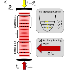
Figure 1: (a) Schematic of a dual-ensemble 1D Yb OLC (not to scale). The 759 nm lattice is formed via retro-reflection of a single beam and clock light is introduced through the mirror used for reflection of the 759 nm beam. The directions of the polarization, magnetic field, and gravity orientation are indicated. (b) A 759 nm transverse running wave may be introduced to ensemble 2, allowing evaluation of the running wave magic wavelength and hyperpolarizability via differential comparisons. (c) The longitudinal motional state of the atoms in each ensemble may be manipulated separately, providing enhanced, differential sensitivity to higher-order light shift terms.

Near the magic wavelength, the lattice light shift $\delta\nu_{LS}$ can be written as a function of trap depth $U$, detuning $\delta_{L}$ of lattice frequency $\nu_{L}$ from the electric dipole ($E1$) magic frequency $\nu_{E1}$ ($\delta_{L}=\nu_{L}-\nu_{E1}$), radial temperature $T_{r}$, and longitudinal vibrational state $n_{z}$. For simplicity we follow Ref. [18], adopting a light shift model utilizing a harmonic basis (see Appendix A for a complementary treatment with a more general model). The lattice light shift is then given by

$$\frac{\delta\nu_{LS}(u,\delta_{L},n_{z})}{\nu_{c}}\approx \bigg{(}\frac{\partial\tilde{\alpha}_{E1}}{\partial\nu}\delta_{L}-\tilde{\alpha}_{M1E2}\bigg{)}\bigg{(}n_{z}+1/2\bigg{)}u^{1/2}$$ (1)

$$-\bigg{[}\frac{\partial\tilde{\alpha}_{E1}}{\partial\nu}\delta_{L}+\frac{3}{2}\tilde{\beta}\bigg{(}n_{z}^{2}+n_{z}+\frac{1}{2}\bigg{)}\bigg{]}u$$

$$+2\tilde{\beta}\bigg{(}n_{z}+\frac{1}{2}\bigg{)}u^{3/2}-\tilde{\beta}u^{2},$$

where we have divided the clock shift ($\delta\nu_{LS}$) by the clock frequency ($\nu_{c}$) and utilize normalized trap depths $u=U/E_{R}$. $E_{R}=(h\nu_{L})^{2}/2mc^{2}$ is the recoil energy and $c$ the speed of light, $m$ the atomic mass, and $h$ Planck’s constant. The effects of transverse temperatures are captured via an effective depth $u^{j}\rightarrow(1+jk_{B}T_{r}/uE_{R})^{-1}u^{j}$ [18, 30] where $j$ is the power series exponent for each term in Eq. (1). $k_{B}$ is the Boltzmann constant and trap depth is measured via sideband spectroscopy [31]. All trap depths $u^{j}$ in the Letter implicitly assume this effective radial thermal averaging.

Complete lattice light shift evaluations require knowledge of $\nu_{E1}$ and the three differential atomic coefficients within Eq. (1). $\frac{\partial\tilde{\alpha}_{E1}}{\partial\nu}$ is the linear slope of the differential $E1$ polarizability between the ground (¹S₀) and excited (³P₀) clock states arising from a Taylor expansion about $\nu_{E1}$. $\tilde{\alpha}_{M1E2}$ and $\tilde{\beta}$ are the differential multipolarzability and hyperpolarizability, respectively. These coefficients are often evaluated via interleaved comparisons between two trap depths ($u$) [32] or two motional states ($n_{z}$) [18]. By operating over a broad range of trap depths, lattice frequencies, and motional states, individual polarizability terms can be disentangled and measured. In many OLCs, however, practical limits of the realizable trap depths make such an evaluation daunting at the state-of-the-art level. Here, we overcome this limitation by supplementing the standard evaluation techniques with imaging and multi-ensemble operation.

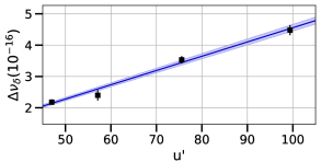
Figure 2: $\frac{\partial\tilde{\alpha}_{E1}}{\partial\nu}$ is measured by temporally self-interleaving between lattice frequency detunings $\delta_{2}$ and $\delta_{1}$ for a single ensemble. The frequency shift, with error bars derived from the Allan deviation at half the total measurement time, is plotted versus $u^{\prime}$. A linear fit, with 1-$\sigma$ error bars (shaded region), gives $\frac{\partial\tilde{\alpha}_{E1}}{\partial\nu}$ as the slope.

Evaluation of $\partial\tilde{\alpha}_{E1}/\partial\nu$.–The only terms in Eq. (1) that include $\partial\tilde{\alpha}_{E1}/\partial\nu$ are proportional to $\delta_{L}$. Therefore, self-interleaved measurements of the light shift at two lattice detunings $\delta_{1}$ and $\delta_{2}$ allow $\frac{\partial\tilde{\alpha}_{E1}}{\partial\nu}$ to be isolated. With the same initial preparation conditions, the frequency difference is

$$\frac{\Delta\nu_{\delta}(u,\delta_{1},\delta_{2},n_{z})}{\nu_{c}} =-\frac{\partial\tilde{\alpha}_{E1}}{\partial\nu}\big{(}\delta_{2}-\delta_{1}\big{)}u^{\prime},$$ (2)

where we have introduced $u^{\prime}=[u-(n_{z}+1/2)u^{1/2}]$. Critically, such a measurement is independent of $\tilde{\alpha}_{M1E2}$, $\tilde{\beta}$, and $\nu_{E1}$, while also benefiting from identical atom preparation to differentially reject cold collision shifts. As shown in Fig. 2, we perform these measurements at four trap depths with $\delta_{2}-\delta_{1}=-108.2(2)$ MHz and find $\frac{\partial\tilde{\alpha}_{E1}}{\partial\nu}=4.2(1)\times 10^{-20}$/MHz, in excellent agreement with previous measurements [2, 33].

Evaluation of $\tilde{\beta}$.–We now turn to the remaining atomic coefficients in Eq. (1). At the limited trap depths available in our apparatus ($<140$ $E_{R}$), evaluation of these shifts with standard interleaved measurements is challenging. Instead, we utilize imaging and dual-ensemble operation as shown in Fig. 1. Frequency comparisons between the two ensembles (found by converting differences in excitation probabilities to frequency via the known Rabi lineshape [29]) are insensitive to laser frequency-noise, providing enhanced relative stability [24, 8]. We regularly measure frequency instabilities of $\sim 4\times 10^{-17}$ at 1 s for synchronous comparison between ensembles as compared with $\sim 3\times 10^{-16}$ for temporally self-interleaved measurements, allowing us to evaluate shifts nearly 50 times faster.

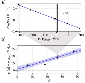
Figure 3: Measurement of the running wave magic frequency, $\nu_{r}^{\prime}(u^{\prime})$. (a) The frequency shift arising from the addition of a running wave, measured synchronously, is plotted versus the running wave frequency, $\nu_{r}$. Error bars are smaller than the point size and $\nu_{\mathrm{offset}}=394~{}798~{}300$ MHz. We show the fit for a $u^{\prime}=54$ standing wave contribution with black lines showing the fitted intercept for $\nu_{r}^{\prime}(u^{\prime})$. (b) $\nu_{r}^{\prime}(u^{\prime})$ is plotted versus $u^{\prime}$ for each of the four evaluated depths. The blue line and associated 1-$\sigma$ statistical uncertainty region show the fit to Eq. (4).

We apply an auxiliary running wave field to the second ensemble (Fig. 1(b)), near the magic frequency (but $>$MHz detuned from the standing wave laser frequency). For a running wave the $E1$ polarizability and multipolarizability terms simply add, in contrast to a standing wave where they are out of phase. The fractional frequency shift from the addition of an auxiliary running wave to the standing wave is

$$\frac{\delta\nu_{R}(u_{r},u^{\prime},\delta_{r})}{\nu_{c}} \approx-\bigg{(}\frac{\partial\tilde{\alpha}_{E1}}{\partial\nu}\delta_{r}+\tilde{\alpha}_{M1E2}+\tilde{\beta}_{d}u^{\prime}\bigg{)}u_{r},$$ (3)

where $u_{r}$ is the running wave ‘depth’, $u^{\prime}$ the average standing wave depth experienced by the atoms (as introduced in Eq. (2)), $\delta_{r}=\nu_{r}-\nu_{E1}$, and $\nu_{r}$ the running wave frequency (note that shifts of order $u_{r}^{2}$ and higher have been omitted here [29]). Equation (3) includes a shift term that is $\propto u^{\prime}u_{r}$, arising from the dichromatic hyperpolarizability $\tilde{\beta}_{d}$ [34, 35]. For parallel linear lattice and running wave polarizations (Fig. 1), the dichromatic hyperpolarzability is related to the more familiar hyperpolarzability of Eq. (1) by $\tilde{\beta}_{d}=4\tilde{\beta}$ [35]. This interference effect provides a new method to determine $\tilde{\beta}$ with minimal correlation to $\nu_{E1}$ [32]. Further, the use of synchronous dual-ensemble measurements facilitates its precise determination at shallow lattice depths. The auxiliary field has a $u^{\prime}$-dependent frequency $\nu_{r}^{\prime}(u^{\prime})$ where $\delta\nu_{R}(u_{r},u^{\prime},\nu^{\prime}_{r}-\nu_{E1})=0$, given by

$$\nu_{r}^{\prime}(u^{\prime})=\bigg{(}\nu_{E1}-\frac{\tilde{\alpha}_{M1E2}}{\frac{\partial\tilde{\alpha}_{E1}}{\partial\nu}}\bigg{)}-\frac{4\tilde{\beta}u^{\prime}}{\frac{\partial\tilde{\alpha}_{E1}}{\partial\nu}}.$$ (4)

$\nu_{r}^{\prime}(u^{\prime})$ is a linear function of $u^{\prime}$ with a slope revealing $\tilde{\beta}$ and an offset $\nu_{r}^{\prime}(0)=\nu_{E1}-\tilde{\alpha}_{M1E2}/\frac{\partial\tilde{\alpha}_{E1}}{\partial\nu}$, directly relating $\nu_{E1}$ and $\tilde{\alpha}_{M1E2}$.

To experimentally evaluate $\nu_{r}^{\prime}(u^{\prime})$ we apply a running wave beam with a waist of $\approx 150$ $\mu$m to ensemble 2. We evaluate the ensemble-averaged depth to be $u_{r}\approx 10$, calibrated in-situ by dividing the slope of Fig. 3a by $-\frac{\partial\tilde{\alpha}_{E1}}{\partial\nu}$. In this experiment, we do not apply Sisyphus cooling to lower the radial temperature, unlike all other measurements in this paper, as the addition of the running wave interferes with the optical access used for cooling. At four different standing wave depths the running wave frequency is stepped over 500 MHz centered around the approximate location of $\nu_{r}^{\prime}(u^{\prime})$ (see Fig. 3). From these measurements a linear fit gives $\tilde{\beta}=-1.7(4)\times 10^{-21}$ and $\nu_{r}^{\prime}(0)=394~{}798~{}300.4(18)$ MHz. This value of $\tilde{\beta}$ falls between previous measurements using relatively deep optical lattices [32, 23] and is in good agreement with independent evaluations made via 2-photon resonances [36, 37].

Evaluation of $\tilde{\alpha}_{M1E2}$ and $\nu_{E1}$.–Returning to Fig. 1, we may prepare ensemble 1 in $n_{z}\approx 0$ and ensemble 2 in either $n_{z}\approx 1$ or $n_{z}\approx 2$ [29]. This allows differential comparisons between ensembles to be preferentially sensitive to the $\tilde{\alpha}_{M1E2}$ dominated $\sqrt{u}$ term of Eq. (1). The differential lattice light shift between samples with motional states $n_{1}$ and $n_{2}$ is given by

$$\frac{\Delta\nu_{n}(u,\delta_{r}^{\prime},n_{1},n_{2})}{\nu_{c}}\approx \bigg{(}\frac{\partial\tilde{\alpha}_{E1}}{\partial\nu}\delta_{r}^{\prime}-2\tilde{\alpha}_{M1E2}\bigg{)}\big{(}n_{2}-n_{1}\big{)}u^{1/2}$$ (5)

$$-\frac{3}{2}\tilde{\beta}\bigg{(}n_{2}^{2}+n_{2}-n_{1}^{2}-n_{1}\bigg{)}u$$

$$+2\tilde{\beta}\bigg{(}n_{2}-n_{1}\bigg{)}u^{3/2}$$

with $\delta_{r}^{\prime}=(\nu_{L}-\nu_{r}^{\prime}(0))$. Note the elimination of $\nu_{E1}$ in Eq. (5) by substitution of $\nu_{r}^{\prime}(0)$ into Eq. (1). With the determinations of $\frac{\partial\tilde{\alpha}_{E1}}{\partial\nu}$, $\nu_{r}^{\prime}(0)$, and $\tilde{\beta}$ in hand, this leaves only $\tilde{\alpha}_{M1E2}$ to evaluate.

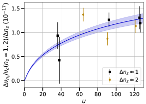
Figure 4: $\tilde{\alpha}_{M1E2}$ is measured via synchronous comparison of $n_{z}\approx 0$ to $n_{z}\approx 1$ (black squares) and to $n_{z}\approx 2$ (gold diamonds). The fit to $\Delta\nu_{n_{z}}/\nu_{c}$, Eq. (5), is shown in blue, with associated 1-$\sigma$ statistical uncertainty shaded. We plot the shifts normalized by $\Delta n_{z}=n_{2}-n_{1}$ to highlight the $\sqrt{u^{\prime}}$ dependence predominantly arising from $\tilde{\alpha}_{M1E2}$. State-preparation errors resulted in $\Delta n_{z}\approx 1\rightarrow 0.8$ and $\Delta n_{z}\approx 2\rightarrow 1.3$ [29]. As a result the plotted fit to Eq. (5) is meant as a visual guide as it assumes perfect state preparation. A Monte-Carlo fit to Eq. (1) for each ensemble is required to fully account for $n_{z}$ and other experimental values, with the results in Table 1. A reduced chi-squared of 1.7 is found.

As shown in Fig. 4, we perform differential $n_{z}$ experiments at a variety of trap depths. The shift is shown normalized by the differential $n_{z}$ applied between ensembles, highlighting the $\sqrt{u}$ dependence (fit shown in blue). The radial temperatures are measured for each ensemble, and $n_{z}$-dependent cold collision corrections are applied [29]. A Monte-Carlo method is used to propagate sources of uncertainty from both measured atomic coefficients and model inputs to the fit of each ensemble to Eq. (1). We find $\tilde{\alpha}_{M1E2}=-1.41(9)\times 10^{-18}$, in good agreement with a previous measurement at lower precision [23]. Finally, $\tilde{\alpha}_{M1E2}$ is substituted back into the definition of $\nu_{r}^{\prime}(0)$, giving $\nu_{E1}=394~{}798~{}266.9(26)$ MHz. Table 1 summarizes our experimental results.

Table 1: Summary of experimental and theoretical values derived from this work. See Appendix A for a complementary Born-Oppenheimer + WKB treatment [30].

Coefficient	Value
$\frac{\partial\tilde{\alpha}_{E1}}{\partial\nu}$ ($10^{-20}$/MHz)	4.2(1)
$\tilde{\beta}$ ($10^{-21}$)	$-1.7(4)$
$\tilde{\alpha}_{M1E2}^{\text{Experiment}}$ $(10^{-18})$	$-1.41(9)$
$\tilde{\alpha}_{M1E2}^{\text{Theory}}$ $(10^{-18})$	$-1.9(5)$
$\nu_{E1}$ (MHz)	$394~{}798~{}266.9(26)$
$\nu^{\prime}_{r}(0)$ (MHz)	$394~{}798~{}300.4(18)$

Theoretical predictions of $\tilde{\alpha}_{M1E2}$.–It is now recognized that earlier calculations for Yb [38, 39, 32], Sr [34, 38, 39, 40, 41], and other alkaline-earth(-like) systems [38, 39, 42, 43, 44, 45] did not include the important diamagnetic contribution to the $M1$ polarizability at the magic wavelength. This resulted in a disagreement between theoretical and experimental results [18, 23, 19, 20], recently resolved in the case of Sr [21, 22]. The diamagnetic shift has been discussed extensively in the literature for the case of uniform dc magnetic fields (e.g., Refs. [46, 47, 48]). In a nonrelativistic treatment, the diamagnetic shift appears at first order in perturbation theory and is proportional to the expectation value $\langle r^{2}\rangle$, where $r$ denotes the distance from the electron to the nucleus, a sum over all electrons is implied, and a total electronic angular momentum $J=0$ is assumed. In a relativistic treatment starting from the Dirac equation, the emergence of the diamagnetic shift is less conspicuous. It arises at second-order in perturbation theory, being attributed to negative-energy (positron) states in the summation over states. However, it can be reformulated in terms of the expectation value $\langle\beta r^{2}\rangle$, where $\beta$ is a conventional $4\times 4$ Dirac matrix [46, 47]. Evaluated between Dirac bispinors, the operators $r^{2}$ and $\beta r^{2}$ have contributions attributed to large and small components of the Dirac bispinors. The inclusion of $\beta$ merely effects a sign change for the small-component contribution, which vanishes in the nonrelativistic limit [48].

For Yb, we start by considering the differential $M1$ polarizability in the dc limit. Table 2 presents a breakdown of contributions calculated as detailed in the Supplemental Material [29]. The final results are compared to the experimental value, which has a $0.1\%$ uncertainty [2, 49]. As expected, we find that the ${{}^{3}P_{0}}$–${{}^{3}P_{1}}$ “paramagnetic” contribution dominates, in part due to a small energy denominator (i.e., the fine structure splitting) in the second-order summation over states. Meanwhile, we find that the diamagnetic contribution amounts to a $\sim\!2\%$ correction, with other contributions being an order of magnitude smaller still. Though sub-dominant, the diamagnetic contribution is non-negligible in the theory-experiment comparison, exemplifying its role in the differential $M1$ polarizability.

Table 2: $M1$ differential polarizability, evaluated in the dc limit and at the magic frequency. Theoretical contributions include the ${{}^{3}P_{0}}-{{}^{3}P_{1}}$ paramagnetic (positive energy state) contribution, the diamagnetic (negative energy state) contribution, and other smaller contributions. This is an abbreviated version of a more expansive table presented in the Supplemental Material [29], which also includes discussion of theoretical uncertainties. For the dc limit, the final theoretical value is compared to the experimental value. All values are in $10^{-3}$ a.u., where a.u. denotes atomic units based on Gaussian electromagnetic expressions.

contribution	dc limit	magic frequency
${{}^{3}P_{0}}-{{}^{3}P_{1}}$	$5.469$	$-0.016$
diamagnetic	$-0.099$	$-0.099$
other	$0.008$	$-0.002$
total	$5.379(10)$	$-0.116(5)$
expt. [2, 49]	$5.363(6)$

We next consider the differential $M1$ polarizability evaluated at the magic wavelength (see Table 2 and [29]). We find that, relative to the dc limit, the ${{}^{3}P_{0}}$–${{}^{3}P_{1}}$ paramagnetic contribution is largely suppressed, a consequence of the lattice photon energy being much greater than the fine structure splitting. Meanwhile, the dc value for the diamagnetic contribution can be directly applied for the magic wavelength case, as the photon energy is significantly below the energy associated with electron-positron pair production. It follows that the diamagnetic contribution becomes the dominant contribution for the differential $M1$ polarizability at the magic wavelength. Further, evaluating and including the differential $E2$ polarizability at the magic wavelength [29], we obtain the theoretical result $\tilde{\alpha}_{M1E2}=-1.9(5)\times 10^{-18}$, in good agreement with the experimental results (Table 1). Finally, using formalism described in Ref. [40] we found $\tilde{\beta}~{}=-2.3\times 10^{-21}$ in the CI+all-order approximation. In two dominant terms, we replaced the theoretical denominators with more correct experimental ones, that strongly affect the result. We consider the result an order of magnitude estimate.

Summary.–With multi-ensemble operation and imaging, we realize a complete lattice light shift evaluation of a standard retro-reflected 1D OLC using modest trap depths. Our independent evaluation provides valuable atomic coefficients for Yb OLCs while also demonstrating novel techniques for the evaluation of both $\frac{\partial\tilde{\alpha}_{E1}}{\partial\nu}$, $\tilde{\beta}$, and $\tilde{\alpha}_{M1E2}$ [34]. Finally, the experimental and theoretical results from this Letter further validate the recent consensus on the origin of the disagreement on the sign and magnitude of the multipolarizability term $\tilde{\alpha}_{M1E2}$.

Acknowledgments.–We thank K. Kim and A. Staron for careful reading of the manuscript. T.B. acknowledges insightful conversations with A. Goban and R. Hutson. The experimental work was supported by NIST, ONR, and NSF QLCI Grant No. 2016244 and Grant No. 2012117 (KG). T.B. acknowledges support from the NRC RAP. The theoretical work has been supported in part by the US NSF Grants No. PHY-2309254, OMA-2016244, US Office of Naval Research Grant No. N00014-20-1-2513, and by the European Research Council (ERC) under the Horizon 2020 Research and Innovation Program of the European Union (Grant Agreement No. 856415). Calculations in this work were done through the use of Information Technologies resources at the University of Delaware, specifically the high-performance Caviness and DARWIN computer clusters.

I Appendix A: Born-Oppenheimer + WKB Approximation

The lattice light shift model in the main text follows a standard harmonic basis treatment [18]. While it gives important physical intuition, these models are known to break down at higher temperatures as they fail to capture axial-radial couplings [30]. Considering our radial temperature of $\sim 600$ nK ($\sim 1~{}\mu$K in the running wave measurements), we elect to perform an additional analysis using a Born-Oppenheimer+WKB treatment (BO+WKB) which better captures axial-radial couplings [30]. In this treatment the lattice light shift is given by

$$\frac{\delta\nu_{LS}(u,\delta_{L},n_{z},T_{r})}{\nu_{c}}\approx -\sum_{n_{z}}W_{n_{z}}\bigg{[}\frac{\partial\tilde{\alpha}_{E1}}{\partial\nu}\delta_{L}X(n_{z},u_{0},T_{r})u_{0}$$ (6)

$$+\tilde{\alpha}_{M1E2}Y(n_{z},u_{0},T_{r})u_{0}$$

$$+\tilde{\beta}Z(n_{z},u_{0},T_{r})u_{0}^{2}\bigg{]},$$

where $W_{n_{z}}$ is an $n_{z}$ band weight and $u_{0}$ is the peak trap depth normalized by $E_{R}$. $X(n_{z},u_{0},T_{r})$, $Y(n_{z},u_{0},T_{r})$, and $Z(n_{z},u_{0},T_{r})$ are trap depth reduction factors which are numerically calculated [30]. As presented in Table 3, we find good agreement between models, but note a 1-$\sigma$ discrepancy of $\frac{\partial\tilde{\alpha}_{s}{E1}}{\partial\nu}$. We note that future evaluations with improved uncertainties will likely need to utilize colder temperatures to continue to employ the harmonic basis model.

Table 3: Comparison of experimental results as derived from either the harmonic (Eq. (1)) or BO+WKB (Eq. (6)) treatment.

Coefficient	Harmonic Basis	BO+WKB
$\frac{\partial\tilde{\alpha}_{E1}}{\partial\nu}$ ($10^{-20}$/MHz)	4.21(10)	4.31(9)
$\tilde{\beta}$ ($10^{-21}$)	$-1.7(4)$	$-2.0(6)$
$\tilde{\alpha}_{M1E2}^{\text{Experiment}}$ $(10^{-18})$	$-1.41(9)$	$-1.45(8)$
$\nu_{E1}$ (MHz)	$394~{}798~{}266.9(26)$	$394~{}798~{}266.3(30)$
$\nu^{\prime}_{r}(0)$ (MHz)	$394~{}798~{}300.4(18)$	$394~{}798~{}300.0(25)$

References

- Ushijima et al. [2015] I. Ushijima, M. Takamoto, M. Das, T. Ohkubo, and H. Katori, Cryogenic optical lattice clocks, Nature Photonics 9, 185 (2015).
- McGrew et al. [2018] W. McGrew, X. Zhang, R. Fasano, S. Schäffer, K. Beloy, D. Nicolodi, R. Brown, N. Hinkley, G. Milani, M. Schioppo, et al., Atomic clock performance enabling geodesy below the centimetre level, Nature 564, 87 (2018).
- Bothwell et al. [2019] T. Bothwell, D. Kedar, E. Oelker, J. M. Robinson, S. L. Bromley, W. L. Tew, J. Ye, and C. J. Kennedy, JILA SrI optical lattice clock with uncertainty of 2, Metrologia 56, 065004 (2019).
- Aeppli et al. [2024] A. Aeppli, K. Kim, W. Warfield, M. S. Safronova, and J. Ye, Clock with 8 systematic uncertainty, Phys. Rev. Lett. 133, 023401 (2024).
- Schioppo et al. [2017] M. Schioppo, R. C. Brown, W. F. McGrew, N. Hinkley, R. J. Fasano, K. Beloy, T. Yoon, G. Milani, D. Nicolodi, J. Sherman, et al., Ultrastable optical clock with two cold-atom ensembles, Nature Photonics 11, 48 (2017).
- Oelker et al. [2019] E. Oelker, R. Hutson, C. Kennedy, L. Sonderhouse, T. Bothwell, A. Goban, D. Kedar, C. Sanner, J. Robinson, G. Marti, et al., Demonstration of 4.8 stability at 1 s for two independent optical clocks, Nature Photonics 13, 714 (2019).
- Zheng et al. [2022] X. Zheng, J. Dolde, V. Lochab, B. N. Merriman, H. Li, and S. Kolkowitz, Differential clock comparisons with a multiplexed optical lattice clock, Nature 602, 425 (2022).
- Bothwell et al. [2022] T. Bothwell, C. J. Kennedy, A. Aeppli, D. Kedar, J. M. Robinson, E. Oelker, A. Staron, and J. Ye, Resolving the gravitational redshift across a millimetre-scale atomic sample, Nature 602, 420 (2022).
- Dimarcq et al. [2024] N. Dimarcq, M. Gertsvolf, G. Mileti, S. Bize, C. Oates, E. Peik, D. Calonico, T. Ido, P. Tavella, F. Meynadier, et al., Roadmap towards the redefinition of the second, Metrologia 61, 012001 (2024).
- Derevianko and Pospelov [2014] A. Derevianko and M. Pospelov, Hunting for topological dark matter with atomic clocks, Nature Physics 10, 933 (2014).
- Kennedy et al. [2020] C. J. Kennedy, E. Oelker, J. M. Robinson, T. Bothwell, D. Kedar, W. R. Milner, G. E. Marti, A. Derevianko, and J. Ye, Precision metrology meets cosmology: improved constraints on ultralight dark matter from atom-cavity frequency comparisons, Phys. Rev. Lett. 125, 201302 (2020).
- Takamoto et al. [2020] M. Takamoto, I. Ushijima, N. Ohmae, T. Yahagi, K. Kokado, H. Shinkai, and H. Katori, Test of general relativity by a pair of transportable optical lattice clocks, Nature photonics 14, 411 (2020).
- Zheng et al. [2023] X. Zheng, J. Dolde, M. C. Cambria, H. M. Lim, and S. Kolkowitz, A lab-based test of the gravitational redshift with a miniature clock network, Nature Communications 14, 4886 (2023).
- Mehlstäubler et al. [2018] T. E. Mehlstäubler, G. Grosche, C. Lisdat, P. O. Schmidt, and H. Denker, Atomic clocks for geodesy, Reports on Progress in Physics 81, 064401 (2018).
- Takamoto and Katori [2003] M. Takamoto and H. Katori, Spectroscopy of the 1SP0 clock transition of Sr87 in an optical lattice, Phys. Rev. Lett. 91, 223001 (2003).
- Ye et al. [2008] J. Ye, H. Kimble, and H. Katori, Quantum state engineering and precision metrology using state-insensitive light traps, science 320, 1734 (2008).
- Taichenachev et al. [2008] A. Taichenachev, V. Yudin, V. Ovsiannikov, V. Pal’Chikov, and C. W. Oates, Frequency shifts in an optical lattice clock due to magnetic-dipole and electric-quadrupole transitions, Phys. Rev. Lett. 101, 193601 (2008).
- Ushijima et al. [2018] I. Ushijima, M. Takamoto, and H. Katori, Operational magic intensity for Sr optical lattice clocks, Phys. Rev. Lett. 121, 263202 (2018).
- Dörscher et al. [2023] S. Dörscher, J. Klose, S. Maratha Palli, and C. Lisdat, Experimental determination of the polarizability of the strontium clock transition, Phys. Rev. Res. 5, L012013 (2023).
- Kim et al. [2023a] K. Kim, A. Aeppli, T. Bothwell, and J. Ye, Evaluation of lattice light shift at low uncertainty for a shallow lattice Sr optical clock, Phys. Rev. Lett. 130, 113203 (2023a).
- Wu et al. [2023a] F.-F. Wu, T.-Y. Shi, W.-T. Ni, and L.-Y. Tang, Contribution of negative-energy states to the polarizability of optical clocks, Phys. Rev. A 108, L051101 (2023a).
- Porsev et al. [2023] S. Porsev, M. Kozlov, and M. Safronova, Contribution of negative-energy states to multipolar polarizabilities of the Sr optical lattice clock, Phys. Rev. A 108, L051102 (2023).
- Nemitz et al. [2019] N. Nemitz, A. A. Jørgensen, R. Yanagimoto, F. Bregolin, and H. Katori, Modeling light shifts in optical lattice clocks, Phys. Rev. A 99, 033424 (2019).
- Marti et al. [2018] G. E. Marti, R. B. Hutson, A. Goban, S. L. Campbell, N. Poli, and J. Ye, Imaging optical frequencies with 100 Hz precision and 1.1 m resolution, Phys. Rev. Lett. 120, 103201 (2018).
- Manovitz et al. [2019] T. Manovitz, R. Shaniv, Y. Shapira, R. Ozeri, and N. Akerman, Precision measurement of atomic isotope shifts using a two-isotope entangled state, Phys. Rev. Lett. 123, 203001 (2019).
- Kim et al. [2023b] M. E. Kim, W. F. McGrew, N. V. Nardelli, E. R. Clements, Y. S. Hassan, X. Zhang, J. L. Valencia, H. Leopardi, D. B. Hume, T. M. Fortier, A. D. Ludlow, and D. R. Leibrandt, Improved interspecies optical clock comparisons through differential spectroscopy, Nature Physics 19, 25 (2023b).
- Chen et al. [2024] C.-C. Chen, J. L. Siegel, B. D. Hunt, T. Grogan, Y. S. Hassan, K. Beloy, K. Gibble, R. C. Brown, and A. D. Ludlow, Clock-line-mediated sisyphus cooling, Phys. Rev. Lett. 133, 053401 (2024).
- Hassan et al. [2024] Y. S. Hassan, T. Kobayashi, T. Bothwell, J. L. Siegel, B. D. Hunt, K. Beloy, K. Gibble, T. Grogan, and A. Ludlow, Ratchet loading and multi-ensemble operation in an optical lattice clock, Quantum Science and Technology (2024).
- [29] See Supplemental Material at [editor insert url].
- Beloy et al. [2020] K. Beloy, W. McGrew, X. Zhang, D. Nicolodi, R. J. Fasano, Y. Hassan, R. Brown, and A. Ludlow, Modeling motional energy spectra and lattice light shifts in optical lattice clocks, Phys. Rev. A 101, 053416 (2020).
- Blatt et al. [2009] S. Blatt, J. W. Thomsen, G. K. Campbell, A. D. Ludlow, M. D. Swallows, M. J. Martin, M. M. Boyd, and J. Ye, Rabi spectroscopy and excitation inhomogeneity in a one-dimensional optical lattice clock, Phys. Rev. A 80, 052703 (2009).
- Brown et al. [2017] R. C. Brown, N. B. Phillips, K. Beloy, W. F. McGrew, M. Schioppo, R. J. Fasano, G. Milani, X. Zhang, N. Hinkley, H. Leopardi, et al., Hyperpolarizability and operational magic wavelength in an optical lattice clock, Phys. Rev. Lett. 119, 253001 (2017).
- Kim et al. [2021] H. Kim, M.-S. Heo, C. Y. Park, D.-H. Yu, and W.-K. Lee, Absolute frequency measurement of the 171Yb optical lattice clock at KRISS using TAI for over a year, Metrologia 58, 055007 (2021).
- Ovsiannikov et al. [2013] V. Ovsiannikov, V. Pal’Chikov, A. Taichenachev, V. Yudin, and H. Katori, Multipole, nonlinear, and anharmonic uncertainties of clocks of Sr atoms in an optical lattice, Phys. Rev. A 88, 013405 (2013).
- Beloy [2024] K. Beloy, In Preparation (2024).
- Kobayashi et al. [2018] T. Kobayashi, D. Akamatsu, Y. Hisai, T. Tanabe, H. Inaba, T. Suzuyama, F.-L. Hong, K. Hosaka, and M. Yasuda, Uncertainty evaluation of an 171Yb optical lattice clock at NMIJ, IEEE Transactions on Ultrasonics, Ferroelectrics, and Frequency Control 65, 2449 (2018).
- Pizzocaro et al. [2020] M. Pizzocaro, F. Bregolin, P. Barbieri, B. Rauf, F. Levi, and D. Calonico, Absolute frequency measurement of the transition of 171Yb with a link to international atomic time, Metrologia 57, 035007 (2020).
- Katori et al. [2015] H. Katori, V. D. Ovsiannikov, S. I. Marmo, and V. G. Palchikov, Strategies for reducing the light shift in atomic clocks, Phys. Rev. A 91, 052503 (2015).
- Ovsiannikov et al. [2016] V. D. Ovsiannikov, S. I. Marmo, V. G. Palchikov, and H. Katori, Higher-order effects on the precision of clocks of neutral atoms in optical lattices, Phys. Rev. A 93, 043420 (2016).
- Porsev et al. [2018] S. G. Porsev, M. S. Safronova, U. I. Safronova, and M. G. Kozlov, Multipolar polarizabilities and hyperpolarizabilities in the Sr optical lattice clock, Phys. Rev. Lett. 120, 063204 (2018).
- Wu et al. [2019] F.-F. Wu, Y.-B. Tang, T.-Y. Shi, and L.-Y. Tang, Dynamic multipolar polarizabilities and hyperpolarizabilities of the Sr lattice clock, Phys. Rev. A 100, 042514 (2019).
- Ovsiannikov et al. [2017] V. D. Ovsiannikov, S. I. Marmo, S. N. Mokhnenko, and V. G. Palchikov, Higher-order effects on uncertainties of clocks of Mg atoms in an optical lattice, J. Phys.: Conf. Ser. 793, 012020 (2017).
- Wu et al. [2020] F.-F. Wu, Y.-B. Tang, T.-Y. Shi, and L.-Y. Tang, Magic-intensity trapping of the Mg lattice clock with light shift suppressed below , Phys. Rev. A 101, 053414 (2020).
- Porsev and Safronova [2020] S. G. Porsev and M. S. Safronova, Calculation of higher-order corrections to the light shift of the clock transition in Cd, Phys. Rev. A 102, 012811 (2020).
- Wu et al. [2023b] L. Wu, X. Wang, T. Wang, J. Jiang, and C. Dong, Be optical lattice clocks with the fractional Stark shift up to the level of , New J. Phys. 25, 043011 (2023b).
- Szmytkowski [2002] R. Szmytkowski, Larmor diamagnetism and Van Vleck paramagnetism in relativistic quantum theory: The Gordon decomposition approach, Phys. Rev. A 65, 032112 (2002).
- Kutzelnigg [2003] W. Kutzelnigg, Diamagnetism in relativistic theory, Phys. Rev. A 67, 032109 (2003).
- Shiga et al. [2011] N. Shiga, W. M. Itano, and J. J. Bollinger, Diamagnetic correction to the 9Be+ ground-state hyperfine constant, Phys. Rev. A 84, 012510 (2011).
- [49] The quadratic Zeeman shift coefficient for the clock transition is reported as in Ref. [2]. Here, we report a corrected value of , as discussed in the Supplemental Material [29].
- Dzuba and Derevianko [2010] V. A. Dzuba and A. Derevianko, Dynamic polarizabilities and related properties of clock states of the ytterbium atom, J. Phys. B 43, 074011 (2010).