Uniform Ergodicity and Ergodic-Risk Constrained Policy Optimization

Abstract

In stochastic systems, risk-sensitive control balances performance with resilience to less likely events. Although existing methods rely on finite-horizon risk criteria, this paper introduces ergodic-risk criteria that capture long-term cumulative risks through probabilistic limit theorems. Extending the Linear Quadratic Regulation (LQR) framework, we incorporate constraints on these ergodic-risk criteria derived from the asymptotic behavior of cumulative costs, accounting for extreme deviations. Using tailored Functional Central Limit Theorems (FCLT), we demonstrate that the time-correlated terms in the ergodic-risk criteria converge under strong ergodicity, and establish conditions for convergence in non-stationary settings while characterizing the distribution and providing explicit formulations for the limiting variance of the risk functional. The FCLT is developed by applying ergodic theory for Markov chains and obtaining uniform ergodicity of the controlled process. For quadratic risk functionals on linear dynamics, in addition to internal stability, the uniform ergodicity requires the (possibly heavy-tailed) dynamic noise to have a finite fourth moment. This offers a clear path to quantifying long-term uncertainty. We also propose a primal-dual constrained policy optimization method that optimizes the average performance while ensuring ergodic-risk constraints are satisfied. Our framework offers a practical, theoretically guaranteed approach for long-term risk-sensitive control, backed by convergence guarantees and validations through simulations.

I Introduction

Optimizing average performance, as is typical in standard stochastic optimal control, often fails to yield effective policies for decision making in stochastic environments where deviations from expected outcomes carry significant risk; e.g. in financial markets [1], safe robotics and autonomous systems [2], and healthcare [3]. As such, incorporating risk measures become vital in such decision making problems for balancing the performance with resilience to rare events.

While robust control frameworks (e.g. the mixed $\mathcal{H}_{2}$-$\mathcal{H}_{\infty}$ in [4]), focus on incorporating the worst-case scenario performance (e.g. $\mathcal{H}_{\infty}$-norm) as a constraint, they can be overly conservative, inefficient, or even unfeasible when those unlikely events are (possibly) unbounded. Risk-aware approaches, on the other hand, offer a (probabilistic) compromise by building on available stochastic priors to manage both risk and performance, simultaneously. Consequently, there have been significant efforts [5, 6, 7, 8] in developing risk-aware decision making frameworks using tools like Conditional Value at Risk (CVaR) [1], Markov Risk Measure [9], and Entropic Value at Risk (EVaR) [10], offering a better balance by considering both risk and average performance.

These measures are often deployed on finite-horizon variables and/or in finite state-space models [6, 7, 8]. While avoiding complications regarding limiting probabilities, they may not fully capture long-term risk associated with the stochastic behaviors, especially in unbounded general-state Markov processes pertaining to applications of our interest; also see the recent survey [11]. Also at the stationary limits of the process, the optimal policy that minimizes the worst-case CVaR of the quadratic cost is shown to be equivalent to that of the Linear Quadratic Regulators (LQR) optimal [12]. This is yet another evidence suggesting that risk-sensitive design is particularly critical in nonstationary settings. Among these, the folklore risk-sensitive framework by Whittle [5], aka Linear Exponential Quadratic Gaussian (LEQG), handles the general unbounded nonstationary setting–which (in certain parameter regimes) can be interpreted as optimizing a specific mixture of the average performance and its higher moments (e.g. variance). However, the Gaussian noise is critical for the exponentiation to be well-defined, and thus does not capture cases with heavy-tailed noise distributions with rare events. This motivated [13] to introduce a framework for constraining the uncertainty in the “state-related portion” of the finite-horizon LQR cost, which is then extended to infinite-horizon through policy optimization techniques [14].

This paper considers the stochastic Linear Time Invariant (LTI) model with process noise having bounded moments up to the fourth order, prototyping a framework for risk-aware decision-making in unbounded, nonstationary Markov processes with (possibly) heavy-tailed noise. We introduce ergodic-risk criteria, using limit theorems in probability to address risks in the long-term stochastic behavior, focusing on extreme deviations beyond mean performance (Section II). By incorporating stochastic stability of the process and ergodic theory [15], we manage system state correlations in the ergodic-risk criteria to establish their well-definiteness through Functional Central Limit Theorems tailored in Theorem 11. This enables us to address long-term risk in non-stationary processes, previously excluded from the literature (see e.g. [12]). Lastly, we propose a constrained policy optimization framework using strong duality in primal-dual methods that optimizes average performance while meeting ergodic-risk constraints (Section V), with a convergence guarantee and validations through simulations (Section V-D). Our ergodic-risk framework generalizes that of [14] in which the risk functional does not explicitly depend on the input signal (see Section V-A).

Our contributions are as follows:

• Formalizing Ergodic-Risk Criteria: We introduce a novel ergodic-risk criterion as an extension of risk-sensitive control, capturing long-term cumulative risks through probabilistic limit theorems. This formulation accounts for extreme deviations in the system’s performance over time.

• Convergence and Distribution Characterization Using Functional Central Limit Theorems (FCLT): Using tailored FCLT, we demonstrate that time-correlated terms in the ergodic-risk criteria converge under strong ergodicity. We establish conditions for this convergence in non-stationary settings and provide explicit formulations for the limiting variance of the risk functional. The FCLT is developed by applying ergodic theory for Markov chains and obtaining uniform ergodicity of the controlled process. For quadratic risk functionals on linear dynamics, uniform ergodicity, in addition to internal stability, requires the dynamic noise to have a finite fourth moment, even if it is heavy-tailed.

• Control Synthesis Integration: We integrate the ergodic-risk criterion into a control synthesis framework, enabling its practical application in long-term risk-aware control for stochastic systems, specifically those with unbounded state spaces and non-stationary dynamics.

• Primal-Dual Constrained Policy Optimization: By first establishing a strong duality, we propose a constrained policy optimization framework based on a primal-dual method that optimizes the system’s average performance while satisfying ergodic-risk constraints. This method is supported by a convergence guarantee and is validated through simulations. Our framework generalizes that of [14] in which the risk functional does not explicitly depend on the input signal.

The rest of the paper is organized as follows:

In Section II, we present the background and problem setup, defining the stochastic linear time-invariant (LTI) model and introducing the ergodic-risk criterion. This section formalizes the risk-sensitive control framework, providing the foundational aspects of the problem. In Section III, we conduct a detailed theoretical analysis of the ergodic-risk criterion, demonstrating its convergence properties using tailored Functional Central Limit Theorems (FCLT). We apply ergodic theory and establish the uniform ergodicity of the controlled process. Section IV integrates the ergodic-risk criterion into a control synthesis framework, showing how it can be applied to manage long-term risks in stochastic systems. In Section V, We also explore the strong duality properties of the proposed constrained policy optimization framework, and develop a primal-dual method that optimizes average performance while satisfying ergodic-risk constraints. Finally, in Section V-D, we validate the framework through simulations and discuss the convergence guarantees of the proposed algorithms, concluding with insights for future research directions in Section VI.

II Background and Problem Setup

Consider the discrete-time stochastic linear system,

$${X}_{t+1}=A{X}_{t}+B{U}_{t}+H{W}_{t+1}$$ (1)

where $A\in\mathbb{R}^{n\times n}$, $B\in\mathbb{R}^{n\times m}$, and $H\in\mathbb{R}^{n\times d}$ are system parameters, i.e., $n\times n$, $n\times m$, and $n\times d$ real matrices, ${X}_{t}$ and ${U}_{t}$ denote the state and input vectors, respectively. Also, ${W}_{t}$ is denoting the mean-zero process noise and ${X}_{0}$ is the initial state vectors that are sampled from probability distributions $\mathbb{P}_{{W}}$ and $\mathbb{P}_{0}$ with covariances $\Sigma_{W}$ and $\Sigma_{0}$, respectively. We denote the mean of initial distribution by $m_{0}={\mathbb{E}\,}({X}_{0})$. We denote the history of state-input trajectory up to time $t$ by ${\mathcal{H}}_{t}=\{{X}_{j},{U}_{j}\}_{j=0}^{t}$ and $\mathcal{F}_{t}=\sigma({\mathcal{H}}_{t})$ denotes the $\sigma$-algebra generated by ${\mathcal{H}}_{t}$. Note that each ${W}_{t}$ is measurable with respect to $\mathcal{F}_{t}$, which we denote by ${W}_{t}\in\mathcal{F}_{t}$. Let $\mathcal{F}_{-1}$ be the trivial $\sigma$-algebra, then at each time $t\geq 0$, we apply an admissible input signal ${U}_{t}\in\mathcal{L}_{2}(\mathcal{F}_{t-1}\vee\sigma\{{X}_{t}\})$ (i.e. measurable with respect to the smallest $\sigma$-algebra containing both $\mathcal{F}_{t-1}$ and $\sigma\{{X}_{t}\}$) and measure the next stochastic state vector ${X}_{t+1}$.

Intuitively, we require the process noise and initial states to be uncorrelated across time, i.e.,

$${X}_{0}\perp{W}_{t},\text{ and }{W}_{t}\perp{W}_{s},\quad\forall t,s\geq 1.$$

In particular, for each $t\geq 0$, the process noise ${W}_{t}$ is independent of $\mathcal{F}_{t-1}$, but (by definition) measurable with respect to $\mathcal{F}_{t}$. For simplicity, we pose the following stronger assumption.

Assumption 1.

The sequence $\{{W}_{t}\}$ consists of i.i.d. samples of a common zero-mean probability measure $\mathbb{P}_{w}$ that is non-singular with respect to Lebesgue measure $\lambda$ on $\mathbb{R}^{d}$, has a non-trivial density, and has finite second moment (with covariance $\Sigma_{W}\succ 0$).

Given an input signal ${U}=\{{U}_{t}\}_{t=0}^{T}$, we define the cumulative cost

$$J_{T}({U})=\sum_{t=0}^{T}{X}_{t}^{\intercal}Q{X}_{t}+{U}_{t}^{\intercal}R{U}_{t},$$ (2)

with $Q\succeq 0$ and $R\succ 0$ being positive semidefinite and positive definite matrices, respectively. Conventionally, the infinite-horizon Linear Quadratic Regulators (LQR) problem is to design a sequence of admissible inputs ${U}=\{{U}_{t}\}_{0}^{\infty}$ that minimizes

$$J({U})=\limsup_{T\to\infty}\frac{1}{T}{\mathbb{E}\,}[J_{T}({U})],$$

subject to dynamics in Equation 1. It is well known that the optimal solution to this problem reduces to solving the Discrete-time Algebraic Riccati Equation (DARE)

$$P_{\mathrm{LQR}}=A^{\intercal}P_{\mathrm{LQR}}A+Q\\ -A^{\intercal}P_{\mathrm{LQR}}B(R+B^{\intercal}P_{\mathrm{LQR}}B)^{-1}B^{\intercal}P_{\mathrm{LQR}}A,$$

for the unknown matrix $P_{\mathrm{LQR}}$ that quadratically parameterizes the so-called cost-to-go. Subsequently, one sets ${U}_{t}^{*}=K_{\mathrm{LQR}}{X}_{t}$, where the optimal LQR gain (policy) $K_{\mathrm{LQR}}\in\mathbb{R}^{m\times n}$ is given by $K_{\mathrm{LQR}}=-(R+B^{\intercal}P_{\mathrm{LQR}}B)^{-1}B^{\intercal}P_{\mathrm{LQR}}A,$ and the optimal cost $J({U}^{*})=\mathrm{tr}\left[P_{\mathrm{LQR}}\Sigma_{W}\right]$ with $\Sigma_{W}$ denoting the covariance of $\mathbb{P}_{{W}}$. Note that $\Sigma_{0}$ will not affect the optimal cost.

Lastly, we set some terminologies. A policy $\pi=\{\pi_{t}\}_{t}$ is a collection measurable mappings that generate an input sequence $\{{U}_{t}=\pi_{t}({\mathcal{H}}_{t-1},{X}_{t})\}_{t}$ such ${U}_{t}$ is admissible for all time $t$. A policy is Markov if it does not depend on the history ${\mathcal{H}}_{t-1}$ for every $t$, and called stationary if it is independent of time $t$. So, the optimal LQR policy is a stationary Markov policy, and this work we also restrict ourselves to the class of affine stationary Markov policies.

II-A Ergodic-Risk Criterion for Stochastic Systems

We propose a risk criterion that captures the long-term uncertainty by accumulating step-wise uncertainties as the system evolves. Since each state ${X}_{t}$ is observed iteratively, it is natural to consider the uncertainty at each stage and accumulate these contributions over time to characterize the overall risk. This leads to a cumulative uncertainty variable, which converges to a limiting value if properly normalized.

To formalize this, let us consider any measurable functional of choice $g:\mathbb{R}^{n}\times\mathbb{R}^{m}\mapsto\mathbb{R}$, called “risk functional,” for example a quadratic/affine function in ${X}_{t}$ and/or ${U}_{t}$ which evaluates the performance of each sample path (possibly different than the performance cost). At each time $t-1$, we have access to information in $\mathcal{F}_{t-1}$, so the risk factor at time $t$ is the “uncertain component” of the risk functional $g({X}_{t},{U}_{t})$. This motivates the following definition

$$C_{t}\coloneqq g({X}_{t},{U}_{t})-{\mathbb{E}\,}[g({X}_{t},{U}_{t})|\mathcal{F}_{t-1}],\quad\text{for $t\geq 0$,}$$ (3)

capturing the uncertainty in $g({X}_{t},{U}_{t})$ relative to that past information—see Figure 1. To account for the long-term risk behavior, especially in non-stationary systems with heavy-tailed noise, we define the ergodic-risk criterion $C_{\infty}$ as the limit of the normalized cumulative uncertainty:

$$\frac{1}{\sqrt{t}}S_{t}\coloneqq\frac{1}{\sqrt{t}}\sum_{s=0}^{t}C_{s}\xrightarrow{d\;}C_{\infty},\quad t\to\infty.$$ (4)

We also consider the asymptotic conditional variance $\gamma_{N}^{2}$ defined as the limit

$$\frac{1}{t}N_{t}\coloneqq\frac{1}{t}\sum_{s=1}^{t}{\mathbb{E}\,}[C_{s}^{2}|\mathcal{F}_{s-1}]\xrightarrow{a.s.}\gamma_{N}^{2},\quad t\to\infty,$$ (5)

which would serve as an “estimate” of the asymptotic variance of $C_{\infty}$, whenever well-defined (see Remark 13).

Figure 1: The conditional expectation ${\mathbb{E}\,}[g({X}_{t},{U}_{t})|\mathcal{F}_{t-1}]$ is the orthogonal projection (in blue) of the risk functional $g({X}_{t},{U}_{t})$ onto $\mathcal{L}^{2}(\mathcal{F}_{t-1})$, i.e. its best estimate by the information up to time $t-1$, i.e. the solution to $\arg\min_{\hat{g}\in\mathcal{L}^{2}(\mathcal{F}_{t-1})}\|g-\hat{g}\|_{\mathcal{L}^{2}(\mathcal{F}_{t-1})}=\sqrt{{\mathbb{E}\,}[(g-\hat{g})^{2}]}.$ The random variable $C_{t}$ (in red) then retains the “uncertain part” of the risk functional at time $t$.

Lemma 2.

Suppose

$$|g(x,u)|\leq M(\|x\|^{p}+\|u\|^{p}),\;\forall(x,u)\in\mathbb{R}^{n}\times\mathbb{R}^{m}$$

for some non-negative constants $M,p\geq 1$. Given an affine stationary Markov policy for dynamics equation 1, if the process noise $\{{W}_{t}\}$ and initial condition has finite moments up to order $p$, then $\{C_{t},\mathcal{F}_{t}\}_{0}^{\infty}$ is a Martingale Difference Sequence (MDS); i.e. for all $t$

1. $C_{t}$ is $\mathcal{F}_{t}$-adapted, and

2. ${\mathbb{E}\,}|C_{t}|<\infty$, and

3. ${\mathbb{E}\,}[C_{t}|\mathcal{F}_{t-1}]=0$, a.s. .

Proof.

Note that $g({X}_{t},{U}_{t})\in\mathcal{F}_{t}$ for each $t$. So, $C_{t}$ is $\mathcal{F}_{t}$-adapted. By Conditional Jensen’s Inequality we obtain that for each $t$

$${\mathbb{E}\,}|C_{t}| \leq{\mathbb{E}\,}|g({X}_{t},{U}_{t})|+{\mathbb{E}\,}[{\mathbb{E}\,}[|g({X}_{t},{U}_{t})|\;|\mathcal{F}_{t-1}]]$$

$$=2{\mathbb{E}\,}|g({X}_{t},{U}_{t})|$$

$$\leq 2M\left({\mathbb{E}\,}\|{X}_{t}\|^{p}+{\mathbb{E}\,}\|{U}_{t}\|^{p}\right)<\infty,$$

where the equality follows the Tower property and the last inequality is due to the moment condition on the process noise, the linear dynamics, and the fact that $\pi$ is affine. Because in that case, there exists another constant $M_{2}$ such that

$$\|{X}_{t}\|\leq M_{2}(\|{X}_{t-1}\|+\|{W}_{t}\|+1),$$

$$\|{U}_{t}\|\leq M_{2}(\|{X}_{t-1}\|+1),$$

which by Holder inequality imply that

$$\|{X}_{t}\|^{p}+\|{U}_{t}\|^{p}\leq 3^{p}M_{2}^{p}(\|{X}_{t-1}\|^{p}+\|{W}_{t}\|^{p}+1).$$

If the process noise and initial condition has moments up to order $p$ then ${\mathbb{E}\,}(\|{X}_{t}\|^{p}+\|{U}_{t}\|^{p})$ is bounded for each finite $t$. Finally, ${\mathbb{E}\,}[C_{t}|\mathcal{F}_{t-1}]=0$ by linearity of expectation and Tower property, and thus $\{C_{t},\mathcal{F}_{t}\}$ is a MDS. ∎

Even though, we have shown that $C_{t}$ is a MDS, the well-definiteness of this limiting quantity requires careful analysis of convergence in distribution. Note that the summands are highly correlated through the dynamics in equation 1 and thus vanilla Central Limit Theorem does not apply as it requires independent summands. One can instead apply an extended version of CLT for martingales; e.g. Martingale Central Limit Theorem in [16, Theorem 5.1]. However, even such extension is not useful here because the conditions translates to such strong stability conditions on equation 1 that is not feasible.

II-B A primer on the quadratic case

Next, if we restrict ourselves to the “linear/affine policies” $\pi:x\mapsto Kx+\ell$ for some matrix parameter $K$ and constant vector $\ell$, then each input is designed to be ${U}_{k-1}=K{X}_{k-1}+\ell$. We define the set of (Schur) stabilizing policies as

$$\mathcal{S}=\left\{K\in\mathbb{R}^{m\times n}\;:\;A_{K}\coloneqq A+BK\text{ is Schur stable}\right\},$$

i.e. $A+BK$ has spectral radius less than 1. We refer to $\pi=(K,\ell)\in\mathcal{S}\times\mathbb{R}^{m}$ as the policy without ambiguity. For $\mathcal{S}$ to be non-empty, we consider the following minimal assumption:

Assumption 3.

The pair $(A,B)$ is stabilizable.

Let us define the following processes that become particularly relevant when the risk function is quadratic, i.e. $g(x,u)=x^{\intercal}Q^{c}x+u^{\intercal}R^{c}u$ for some $Q^{c},R^{c}\succeq 0$; namely, the running average and the running covariance

$${\Lambda}_{t} \coloneqq\sum_{s=1}^{t}({X}_{s}-\bar{x}_{K}),\text{ and }$$

$$\Gamma_{t} \coloneqq\sum_{s=1}^{t}({X}_{s}-\bar{x}_{K})({X}_{s}-\bar{x}_{K})^{\intercal},$$ (6)

where

$$\bar{x}_{K}\coloneqq\sum_{\tau=0}^{\infty}A_{K}^{\tau}B\ell.$$ (7)

Now, we can easily argue about the expectation of running average and covariance as follows.

Lemma 4.

Under Assumptions 1 and 3, for any stabilizing affine stationary Markov policy $\pi\in\mathcal{S}\times\mathbb{R}^{m}$, we have the following limits as $t\to\infty$:

$${\mathbb{E}\,}[{X}_{t}]\to\bar{x}_{K},\;{\mathbb{E}\,}[{\Lambda}_{t}/t]\to 0,\\ {\mathbb{E}\,}[\Lambda_{t}/\sqrt{t}]\to 0,\text{ and }{\mathbb{E}\,}[\Gamma_{t}/t]\to\Sigma_{K},$$

where $\Sigma_{K}$ is the unique positive definite solution to the following Lyapunov equation:

$$\Sigma_{K}=A_{K}\Sigma_{K}A_{K}^{\intercal}+H\Sigma_{W}H^{\intercal}.$$ (8)

Furthermore, we have the following convergence in probability:

$${\Lambda}_{t}/t\xrightarrow{p}0,\text{ as }t\to\infty,$$

and the boundedness in probability: there exists absolute constants $\bar{c}_{1},\bar{c}_{2}$ such that for any (large enough) $m$

$$\mathbb{P}(\|{X}_{t}\|\geq m)\leq\bar{c}_{1}/(m-\bar{c}_{2}\|\ell\|)^{2},\quad\forall t\geq 0.$$

Proof.

Note that

$${X}_{t+1}=A_{K}^{t+1}{X}_{0}+\bar{x}_{t}+\sum_{\tau=0}^{t}A_{K}^{t-\tau}H{W}_{\tau+1}$$ (9)

where $\bar{x}_{t}\coloneqq\sum_{\tau=0}^{t}A_{K}^{\tau}B\ell$. By 1 on noise distribution, we observe that

$$\Sigma_{t+1}\coloneqq{\mathbb{E}\,}[({X}_{t+1}-\bar{x}_{t})({X}_{t+1}-\bar{x}_{t})^{\intercal}]$$

must satisfy for all $t\geq 0$:

$$\Sigma_{t+1}=A_{K}^{t+1}\Sigma_{0}(A_{K}^{\intercal})^{t+1}+\sum_{\tau=0}^{t}A_{K}^{\tau}H\Sigma_{W}H^{\intercal}(A_{K}^{\intercal})^{\tau}.$$

As $K\in\mathcal{S}$, $A_{K}$ is stabilizing and so $A_{K}^{t}$ converges to zero geometrically fast as $t$ goes to infinity. Thus, the series is absolutely convergent and we observe that $\Sigma_{t}\to\Sigma_{K}$ where the existence, uniqueness, and positive-definiteness of $\Sigma_{K}$ follows from Discrete Lyapunov Equation. Additionally, as $t\to\infty$ we obtain that $\bar{x}_{t}\to\bar{x}_{K}$, and thus ${\mathbb{E}\,}[{X}_{t+1}]=A_{K}^{t+1}m_{0}+\bar{x}_{t}\to\bar{x}_{K}$. Therefore, for all $t\geq 1$,

$${\mathbb{E}\,}[{\Lambda}_{t}]=\sum_{s=1}^{t}A_{K}^{s}m_{0}+\sum_{s=1}^{t}(\bar{x}_{s-1}-\bar{x}_{K}),$$ (10)

and thus ${\mathbb{E}\,}[{\Lambda}_{t}/t]\to 0$. Note that by exponential stability, both $\sum_{s=1}^{t}(\bar{x}_{s-1}-\bar{x}_{K})$ and $\sum_{s=1}A_{K}^{s}m_{0}$ converge exponentially fast as $t\to\infty$. Thus, by equation 10, ${\mathbb{E}\,}[\Lambda_{t}/\sqrt{t}]\to 0$. Similarly,

$${\mathbb{E}\,}[\Gamma_{t}]=\sum_{s=1}^{t}\Sigma_{s}\\ +\sum_{s=1}^{t}2A_{K}^{s}m_{0}(\bar{x}_{s-1}-\bar{x}_{K})^{\intercal}+(\bar{x}_{s-1}-\bar{x}_{K})(\bar{x}_{s-1}-\bar{x}_{K})^{\intercal}$$ (11)

and thus ${\mathbb{E}\,}[\Gamma_{t}/t]\to\Sigma_{K}$ as $\Sigma_{t}\to\Sigma_{K}$. Next, as ${\mathbb{E}\,}[{X}_{t}]\to\bar{x}_{K}$ exponentially fast, it suffices to show the last claim for the centered process $\{{X}_{t}-\bar{x}_{K}\}$. So consider equation 9 where $\ell=0$ implying the $\bar{x}_{K}=0$ and thus

$${\Lambda}_{t+1} =\sum_{s=0}^{t}{X}_{s+1}$$

$$=\sum_{s=0}^{t}A_{K}^{s+1}{X}_{0}+\sum_{s=0}^{t}\sum_{\tau=0}^{s}A_{K}^{s-\tau}H{W}_{\tau+1}$$

$$=-{X}_{0}+\sum_{s=-1}^{t}A_{K}^{s+1}{X}_{0}+\sum_{\tau=0}^{t}\sum_{s=\tau}^{t}A_{K}^{s-\tau}H{W}_{\tau+1}$$

$$=-{X}_{0}+\sum_{\tau=-1}^{t}\mathcal{A}_{t-\tau}H{W}_{\tau+1},$$

where $\mathcal{A}_{t}\coloneqq\sum_{s=0}^{t}A_{K}^{s}$ and for simplicity we denote, with abuse of notation, $H{W}_{0}\coloneqq{X}_{0}$. Let us without loss of generality assume $\Sigma_{W}=\Sigma_{0}$ in the rest of the argument. If $K\in\mathcal{S}$, then there exists uniform constants $C,\rho$ such that [17, Lemma 6] $\|A_{K}^{s}\|\leq C\rho^{s},\forall s$, implying that

$$\|\mathcal{A}_{t}\|\leq C\frac{1-\rho^{t}}{1-\rho}\leq\frac{C}{1-\rho}$$

Now, for any $\epsilon>0$, Markov Inequality implies

$$\mathbb{P}\{\|{\Lambda}_{t+1} +{X}_{0}\|>\epsilon t\}$$

$$= \mathbb{P}\{\mathrm{tr}\left[({\Lambda}_{t+1}+{X}_{0})({\Lambda}_{t+1}+{X}_{0})^{\intercal}\right]>\epsilon^{2}t^{2}\}$$

$$\leq \frac{1}{\epsilon^{2}t^{2}}{\mathbb{E}\,}\mathrm{tr}\left[({\Lambda}_{t+1}+{X}_{0})({\Lambda}_{t+1}+{X}_{0})^{\intercal}\right]$$

$$= \frac{1}{\epsilon^{2}t^{2}}{\mathbb{E}\,}\mathrm{tr}\left[\sum_{\tau=-1}^{t}\sum_{s=-1}^{t}\mathcal{A}_{t-\tau}H{W}_{\tau}{W}_{s}^{\intercal}H^{\intercal}\mathcal{A}_{t-s}^{\intercal}\right]$$

$$= \frac{1}{\epsilon^{2}t^{2}}\mathrm{tr}\left[\sum_{s=-1}^{t}\mathcal{A}_{t-s}H\Sigma_{W}H^{\intercal}\mathcal{A}_{t-s}^{\intercal}\right]$$

$$= \frac{1}{\epsilon^{2}t^{2}}\mathrm{tr}\left[H\Sigma_{W}H^{\intercal}\sum_{s=0}^{t+1}\mathcal{A}_{s}^{\intercal}\mathcal{A}_{s}\right]$$

$$\leq \frac{\|H\|^{2}\mathrm{tr}\left[\Sigma_{W}\right]}{\epsilon^{2}t^{2}}\left\|\sum_{s=0}^{t+1}\mathcal{A}_{s}^{\intercal}\mathcal{A}_{s}\right\|$$

$$\leq \frac{\|H\|^{2}\mathrm{tr}\left[\Sigma_{W}\right]}{\epsilon^{2}t^{2}}\sum_{s=0}^{t+1}\left\|\mathcal{A}_{s}\right\|^{2}$$

$$\leq \frac{\|H\|^{2}\mathrm{tr}\left[\Sigma_{W}\right]}{\epsilon^{2}t^{2}}\frac{C^{2}(t+1)}{(1-\rho)^{2}}$$

$$\leq \mathcal{O}(\frac{1}{\epsilon^{2}t})$$

where we used ${\mathbb{E}\,}{{W}_{\tau}{W}_{s}^{\intercal}}=0$ for $\tau\neq s$ and bounded second-order moments of the noise and initial condition. This implies the convergence of ${\Lambda}_{t}/t\xrightarrow{p}0$ in probability. For the last claim, the case of $\ell=0$ follows by a similar argument using Markov Inequality and convergence of $\Sigma_{t}$ and thus, is omitted. For the case of nonzero $\ell$, by [18, Lemma 6], there exists a constant $\bar{c}_{2}$ such that $\|\bar{x}_{t}\|\leq\bar{c}_{2}\|\ell\|$ for all $t\geq 0$. Therefore, $\|{X}_{t}-\bar{x}_{t}\|\geq\|{X}_{t}\|-\bar{c}_{2}\|\ell\|$ which implies that

$$\mathbb{P}(\|{X}_{t}\|\geq m)\leq\mathbb{P}\left(\|{X}_{t}-\bar{x}_{t}\|\geq m-\bar{c}_{2}\|\ell\|\right).$$

This completes the proof. ∎

This allows us to reason about the first and second moment of the process, and also conclude convergence in probability of terms like:

$$\|{X}_{t}\|^{2}/a_{t}\xrightarrow{p}0,$$

for any (scalar deterministic) sequence $a_{t}\to+\infty$ as $t\to\infty$. However, it still does not provide much more for the convergence of $C_{\infty}$ in distribution. In particular, we need much more sophisticated tools to argue about convergence of terms like ${\Lambda}_{t}/\sqrt{t}$, $\Gamma_{t}/\sqrt{t}$, or even $\Gamma_{t}/t$ as $t\to\infty$ (beyond their expectation).

Here, we use another type of extensions to CLT known as “Functional Central Limit Theorem” that extends the Martingale CLT to Markov chains, connecting to their “stochastic stability” properties. Before detailing out this analysis, we discuss the so-called “uniform ergodicity” as a stochastic stability notion that allows for such convergence to hold [15].

III $V$-uniform ergodicity as stochastic stability

We adopt a general-state Markov Decision Process (MDP) perspective. Consider the chain $\mathbf{\Phi}=\{{X}_{t}\}_{0}^{\infty}$ that evolves on the Borel space $(\mathbb{R}^{n},\mathcal{B}(\mathbb{R}^{n}))$ according to the linear state space model Equation 1 for some admissible sequence $\{{U}_{t}\}$. Because $\{{W}_{t}\}$ is i.i.d, then this Markov chain has the following stationary transition kernel

$$P_{u}(x,E)\coloneqq\mathbb{P}\{Ax+Bu+H{W}_{1}\in E\},$$

for any $E\in\mathcal{B}(\mathbb{R}^{n})$. We think of a transition probability kernel as

• for each $E\in\mathcal{B}(\mathrm{X})$, $P_{u}(.,E)$ is a non-negative measurable function on $\mathbb{R}^{n}$, and

• for each $x\in\mathbb{R}^{n}$, $P_{u}(x,.)$ is a probability measure on $\mathcal{B}(\mathbb{R}^{n})$.

Also, $P_{u}$ acts on bounded measurable functions $f$ on $\mathbb{R}^{n}$ as

$$P_{u}(x,f)\coloneqq P_{u}f(x)\coloneqq\int_{\mathbb{R}^{n}}P_{u}(x,dy)f(y),$$

and acts on $\sigma$-finite measures $\mu$ on $\mathcal{B}(\mathbb{R}^{n})$ as

$$\mu P_{u}(E)=\int_{\mathbb{R}^{n}}\mu(dx)P_{u}(x,E).$$

Finally, for any stationary Markov policy $\pi$, we denote the MDP resulting from adopting policy $\pi$ by $\mathbf{\Phi}^{\pi}=\{{X}_{t}\}$ with transition kernel $P_{\pi}$. Also, we inductively define the $n$-step transition kernel

$$P_{\pi}^{n}(x,E)\coloneqq\int_{\mathbb{R}^{n}}P_{\pi(x)}(x,dy)P_{\pi}^{n-1}(y,E),\quad n\geq 2$$

for any $x\in\mathbb{R}^{n},E\in\mathcal{B}(\mathbb{R}^{n})$, with $P_{\pi}(x,E)=P_{\pi(x)}(x,E)$. In particular, for every $x\in\mathbb{R}^{n}$ and $E\in\mathcal{B}(\mathbb{R}^{n})$

$$P_{\pi}(x,E)=\mathbb{P}(Ax+B\pi(x)+{W}_{1}\in E)=\mathbb{P}_{x}\{{X}_{1}\in E\}$$

where ${X}_{1}\in\mathbf{\Phi}^{\pi}$.

The standard ergodic theory establishes conditions for existence of the following limit

$$\lim_{t\to\infty}{\mathbb{E}\,}_{x}[f({X}_{t})]=\sigma(f)\coloneqq\int fd\sigma,$$

for every initial condition and every “bounded function” $f$ on $\mathbb{R}^{n}$, where $\sigma$ is an invariant probability measure, i.e. $\sigma(E)=\sigma P_{u}(E),\;\forall E\in\mathcal{B}(\mathbb{R}^{n})$. To avoid this boundedness assumption, we instead consider the convergence in the $V$-norm, for any (fixed) $V:\mathbb{R}^{n}\mapsto[1,\infty)$, defined as:

$$\|\nu\|_{V}=\sup_{g:|g|\leq V}\left|\nu(g)\coloneqq\int gd\nu\right|$$

where $\nu$ is any signed measure.

Definition 5.

Consider two transition kernels $P_{1},P_{2}$ and consider positive function $V:\mathbb{R}^{n}\to[1,\infty)$. Define the $V$-norm distance:

$$|||P_{1}-P_{2}|||_{V}\coloneqq\sup_{x\in\mathbb{R}^{n}}\frac{\|P_{1}(x,.)-P_{2}(x,.)\|_{V}}{V(x)}.$$

The chain $\mathbf{\Phi}$ is called $V$-uniformly ergodic if

$$|||P^{n}-1\otimes\sigma|||_{V}\to 0,\quad\text{ as }n\to\infty,$$

where the $\otimes$ denotes the outer product of a function and a measure.

We know that $V$-uniformly ergodic chains are always $V$-geometrically ergodic, i.e., there exists $r>1$ such that

$$\sum_{1}^{\infty}r^{n}\|P^{n}(x,.)-\sigma\|_{V}<\infty,\quad\forall x\in\mathbb{R}^{n}.$$

Just like Lyapunov stability, to obtain $V$-uniform ergodicity it is often easier to use a sufficient drift condition known as “Foster-Lyapunov” or its extension as “$f$-modulated drift condition”: We say $\mathbf{\Phi}$ satisfies the $f$-modulated drift condition if for all $x\in\mathbb{R}^{n}$,

$$\Delta V(x)\coloneqq PV(x)-V(x)\leq-f(x)+bI_{C}(x),$$

where $PV(x)\coloneqq{\mathbb{E}\,}\left[V({X}_{t+1})|{X}_{t}=x\right]$. In the special case, where $f(x)=\beta V(x)$ for some $\beta>0$, we call it the geometric drift condition.

This is formalized in the following theorem, but first, we need to introduce the following terminologies:

Definition 6.

A chain $\mathbf{\Phi}=\{{X}_{t}\}$ is called

• (Lebesgue-)irreducible if for any measurable set $E\in\mathcal{B}(\mathbb{R}^{n})$ with positive Lebesgue measure $\lambda(E)>0$

  $$\mathbb{P}_{x}\{\mathbf{\Phi}\text{ ever enters }E\}>0,\;\forall x\in\mathbb{R}^{n};$$

• Harris recurrent if for any $E\in\mathcal{B}(\mathbb{R}^{n})$ with $\lambda(E)>0$

  $$\mathbb{P}_{x}\{\mathbf{\Phi}\in E~{}~{}i.o.\}=1,\;\forall x\in E,$$

  where $\{\mathbf{\Phi}\in E~{}~{}i.o.\}\coloneqq\bigcap_{k=1}^{\infty}\bigcup_{t=k}^{\infty}\{{X}_{t}\in E\}$;

• a T-chain if every compact set is small, i.e., for every compact set $E\in\mathcal{B}(\mathbb{R}^{n})$ there exists $m>0$ and some nontrivial measure $\nu_{m}$ on $\mathcal{B}(\mathbb{R}^{n})$ such that for all $x\in E$ and all $F\in\mathcal{B}(\mathbb{R}^{n})$

  $$P^{m}(x,F)=\mathbb{P}_{x}\{{X}_{m}\in F\}\geq\nu_{m}(F);$$

• positive if it admits a unique invariant probability measure measure $\sigma$, i.e.

  $$\sigma P(E)=\sigma(E),\quad\forall E\in\mathcal{B}(\mathbb{R}^{n});$$

• (strongly-)aperiodic if there exists a $\nu_{1}$-small set with positive $\nu_{1}$-measure, i.e., there exists some set $E\in\mathcal{B}(\mathbb{R}^{n})$ and some nontrivial measure $\nu_{1}$ on $\mathcal{B}(\mathbb{R}^{n})$ such that $\nu_{1}(E)>0$ and for all $x\in E$ and all $F\in\mathcal{B}(\mathbb{R}^{n})$

  $$P(x,F)\geq\nu_{1}(F).$$

Theorem 7 ($f$-norm Ergodic Theorem [15, 14.0.1]).

Suppose the chain $\mathbf{\Phi}=\{{X}_{t}\}$ is Lebesgue-irreducible and strongly aperiodic, and $f:\mathbb{R}^{n}\mapsto[1,\infty)$. The following are equivalent:

• There exists some petite set $C$ and some extended-valued non-negative function $V$ such that $V(x_{0})<\infty$ for some $x_{0}\in\mathbb{R}^{n}$, and the $f$-modulated drift condition holds.

• The chain is positive Harris recurrent with invariant probability $\sigma$ such that $\sigma(f)<\infty$.

In case any of these hold, the chain is $f$-ergodic on $S_{V}=\{x\;:\;V(x)<\infty\}$, i.e. for any $x\in S_{V}$

$$\|P^{k}(x,\cdot)-\sigma\|_{f}\to 0,\quad k\to\infty.$$

If, in addition, $\sigma(V)<\infty$ then there exists a finite constant $B_{f}$ such that for all $x\in S_{V}$

$$\sum_{k=0}^{\infty}\|P^{k}(x,\cdot)-\sigma\|_{f}\leq B_{f}(V(x)+1).$$

It is worth noting that, for positive recurrent chains with invariant probability $\sigma$, the condition $\sigma(f)<\infty$ is critical to obtain ergodicity. Using the Comparison Theorem, we have the following sufficient condition that guarantees $\sigma(f)\leq\sigma(s)$: there exists non-negative, finite-valued functions $V,f$ and $s$ on $\mathbb{R}^{n}$ satisfying

$$\Delta V(x)\leq-f(x)+s(x),\quad\forall x\in\mathbb{R}^{n}.$$

Finally, we restate the following result that enables us characterize $V$-uniform ergodicity by the geometric drift condition:

Theorem 8 ([15, Theorem 16.0.1]).

Suppose that $\mathbf{\Phi}$ is Lebesgue-irreducible and aperiodic. Then the following are equivalent for any $V\geq 1$:

• $\mathbf{\Phi}$ is $V$-uniformly ergodic.

• The geometric drift condition holds for some petite set $C$ and some $V_{0}$, where $V_{0}$ is equivalent to $V$ in the sense that for some $c\geq 1$,

  $$c^{-1}V\leq V_{0}\leq cV.$$

It is worth noting that $V$-uniform ergodicity is invariant of constant multiplication of $V$.

III-A $V$-uniform ergodicity of LTI systems

Now, consider the chain $\mathbf{\Phi}^{\pi}=\{{X}_{t}\}$ representing the closed loop dynamics equation 1 under a policy $\pi=(K,\ell)$ starting from some ${X}_{0}=x$. We next establish the properties defined in Definition 6 for this model which are essentially known except the last form of the uniform ergodicity in fourth power.

Theorem 9.

Suppose Assumptions 1 and 3 holds. Then, for any $\pi\in\mathcal{S}\times\mathbb{R}^{m}$ such that $(A_{K},H)$ is controllable, $\mathbf{\Phi}^{\pi}$ is

• Lebesgue-irreducible, aperiodic T-chain;

• positive, Harris recurrent with a unique invariant probability measure $\sigma_{\pi}$ which is the law of ${X}_{\infty}$ defined as

  $${X}_{\infty}\coloneqq\bar{x}_{K}+\sum_{t=0}^{\infty}A_{K}^{t}HW_{t},$$

  where $\bar{x}_{K}\coloneqq\sum_{\tau=0}^{\infty}A_{K}^{\tau}B\ell$;

• $V$-uniformly ergodic with $V(x)=\|x-\bar{x}_{K}\|_{M}^{2}+1$ for any $M\succ 0$, where $\|x\|_{M}^{2}=x^{\intercal}Mx$;

• $V$-uniformly ergodic with $V(x)=\|x-\bar{x}_{K}\|_{M}^{4}+1$ for any $M\succ 0$, if in addition the noise $\{{W}_{t}\}$ has finite fourth moment.

Proof.

The first claim follows directly from [15, Proposition 6.3.5] whenever $(A_{K},H)$ is controllable. Thus, to show that it is a positive, Harris recurrent chain, by Theorem 7 it suffices to show that the $f$-modulated drift condition holds. Additionally, for the $V$-uniform ergodic property, by Theorem 8 and equivalence of norms (in finite dimensional spaces), overall it suffices to show that the stronger, geometric drift condition holds for the specific $M$ solving the following Lyapunov equation

$$M=A_{K}^{\intercal}MA_{K}+Q,$$

for some $Q\succ I$. Because $A_{K}$ is Schur stable, there exists a unique positive definite $M\succ Q$ solving this Lyapunov equation.

Note that by Lemma 4, ${\mathbb{E}\,}[{X}_{t}]\to\bar{x}_{K}$ for any $\ell\in\mathbb{R}^{m}$. Therefore, it suffices to show the claim for the centered process $\{{X}_{t}-\bar{x}_{K}\}$. Also, the quadratic case of $V(x)=\|x\|_{M}^{2}+1$ is simpler and follows similarly. Thus, we focus on the case $V(x)=\|x\|_{M}^{4}+1$ with $\ell=0$ implying $\bar{x}_{K}=0$. We compute that

$$V( {X}_{t+1})=\|A_{K}{X}_{t}+{W}_{t+1}\|_{M}^{4}+1$$

$$= \left(\|A_{K}{X}_{t}\|_{M}^{2}+\|{W}_{t+1}\|_{M}^{2}+2\langle A_{K}{X}_{t},{W}_{t+1}\rangle\right)^{2}+1$$

$$= \|A_{K}{X}_{t}\|_{M}^{4}+\|{W}_{t+1}\|_{M}^{4}+4|\langle A_{K}{X}_{t},{W}_{t+1}\rangle|^{2}$$

$$+2\|A_{K}{X}_{t}\|_{M}^{2}\|{W}_{t+1}\|_{M}^{2}+4\|A_{K}{X}_{t}\|_{M}^{2}\langle A_{K}{X}_{t},{W}_{t+1}\rangle$$

$$+4\|{W}_{t+1}\|_{M}^{2}\langle A_{K}{X}_{t},{W}_{t+1}\rangle+1$$

$$\leq \|A_{K}{X}_{t}\|_{M}^{4}+\|{W}_{t+1}\|_{M}^{4}+4\|A_{K}{X}_{t}\|_{M}^{2}\|{W}_{t+1}\|_{M}^{2}$$

$$+2\|A_{K}{X}_{t}\|_{M}^{2}\|{W}_{t+1}\|_{M}^{2}+4\|A_{K}{X}_{t}\|_{M}^{2}\langle A_{K}{X}_{t},{W}_{t+1}\rangle$$

$$+4\|{W}_{t+1}\|_{M}^{3}\|A_{K}{X}_{t}\|_{M}+1,$$

where the last inequality follows by Cauchy-Schwarz and the fact that $M\succ Q\succ I$, and so $\|x\|\leq\|x\|_{Q}\leq\|x\|_{M}\leq\lambda_{\max}(M)\|x\|_{Q}$ for all $x\in\mathbb{R}^{n}$. Thus, as ${W}_{t+1}$ is independent of $\mathcal{F}_{t}$, by properties of conditional expectation we obtain for any $x\in\mathbb{R}^{n}$

$$\Delta V( x)={\mathbb{E}\,}[V({X}_{t+1}|{X}_{t}=x)]-V(x)$$

$$\leq \|A_{K}x\|_{M}^{4}-\|x\|_{M}^{4}+m_{4}+4m_{2}\|A_{K}x\|_{M}^{2}$$

$$+2m_{2}\|A_{K}x\|_{M}^{2}+0+4m_{3}\|A_{K}x\|_{M}$$

where $m_{4}={\mathbb{E}\,}\|{W}\|_{M}^{4}$, $m_{3}={\mathbb{E}\,}\|{W}\|_{M}^{3}$, and $m_{2}={\mathbb{E}\,}\|{W}\|_{M}^{2}$. The Lyapunov equation implies that for any $x\in\mathbb{R}^{n}$ that

$$\|A_{K}x\|_{M}^{2}-\|x\|_{M}^{2}=-\|x\|_{Q}^{2},$$

and also $2\|A_{K}x\|_{M}\leq\|A_{K}x\|_{M}^{2}+1$. Thus,

$$\Delta V( x)={\mathbb{E}\,}[V({X}_{t+1}|{X}_{t}=x)]-V(x)$$

$$\leq -\|x\|_{Q}^{2}(\|A_{K}x\|_{M}^{2}+\|x\|_{M}^{2})+m_{4}+2m_{3}$$

$$+(6m_{2}+2m_{3})\|A_{K}x\|_{M}^{2}$$

$$= (6m_{2}+2m_{3}-\|x\|_{Q}^{2})\|A_{K}x\|_{M}^{2}$$

$$+m_{4}+2m_{3}-\|x\|_{Q}^{2}\|x\|_{M}^{2}$$

$$\leq -\frac{1}{2\lambda_{\max}(M)^{4}}V(x)+(6m_{2}+2m_{3}-\|x\|_{Q}^{2})\|A_{K}x\|_{M}^{2}$$

$$+m_{4}+2m_{3}+\frac{1}{2\lambda_{\max}(M)^{4}}-\frac{1}{2}\|x\|_{Q}^{4}$$

where the last inequality follows by $\|x\|_{Q}\leq\|x\|_{M}\leq\lambda_{\max}(M)\|x\|_{Q}$. Now, choose the set $C$ to be

$$C\coloneqq\left\{x\;\big{|}\;\|x\|_{Q}\leq\max\{6m_{2}+2m_{3},1+2m_{4}+4m_{3}\}\right\},$$

and notice that

$$\Delta V(x)\leq-\frac{1}{2\lambda_{\max}(M)^{4}}V(x)+bI_{C}(x),$$

where

$$b\coloneqq m_{4}+2m_{3}+\frac{1}{2}\\ +(6m_{2}+2m_{3})\lambda_{\max}(M)^{2}\max\{6m_{2}+2m_{3},1+2m_{4}+4m_{3}\}^{2},$$

because $\|A_{K}x\|_{M}\leq\|x\|_{M}\leq\lambda_{\max}(M)\|x\|_{Q}$ and $\|x\|_{Q}\leq\max\{6m_{2}+2m_{3},1+2m_{4}+4m_{3}\}$ on $C$. Finally, as long as $\pi$ is stabilizing and the noise has finite fourth moment, $b$ is a uniformly bounded constant and $C$ is a compact measurable set because $x\mapsto\|x\|_{Q}$ is continuous. By the first claim, $\mathbf{\Phi}^{\pi}$ is a Lebesgue-irreducible strongly aperiodic T-chain, and thus $C$ is small set and thus also a petite set. Therefore, the geometric drift condition holds, and the claim follows by Theorem 8.

Finally, in the most general case, one can use the construction of “minimal sub-invariant measures” [15, Theorem 10.4.9] in order to obtain a computable expression for $\sigma_{\pi}$. For the particular LTI case, we provide the following argument which is very similar to [15, Section 10.5.4]. By 1, equation 9 implies that

$${X}_{t+1}\sim A_{K}^{t+1}{X}_{0}+\bar{x}_{t}+\sum_{s=0}^{t}A_{K}^{s}H{W}_{s},$$

i.e. has the same law. But, by Lemma 4, we observe that as $A_{K}$ is stable

$${\mathbb{E}\,}[| {X}_{t+1}|]\leq\|A_{K}^{t+1}\|m_{0}+(\|\bar{x}_{K}\|+{\mathbb{E}\,}[\|W_{1}\|])\sum_{s=0}^{t}\|A_{K}^{s}H\|$$

$$\leq C_{K}m_{0}+(\|\bar{x}_{K}\|+{\mathbb{E}\,}[\|W_{1}\|])\sum_{s=0}^{\infty}\|A_{K}^{s}H\|<\infty,$$

for some constant $C_{K}>0$ where the second inequality follows by [17, Lemma 6] and the last one is due to finite moment condition on $W_{1}$. Thus, Fubini-Tonelli’s Theorem implies that ${X}_{\infty}$ is absolutely convergent and well-defined with

$${\mathbb{E}\,}[|{X}_{\infty}|]\leq(\|\ell\|+{\mathbb{E}\,}[\|W_{1}\|])\sum_{s=0}^{\infty}\|A_{K}^{s}H\|<\infty.$$

Next we show that $\sigma_{\pi}$, as the law of ${X}_{\infty}$, is an invariant measure. Consider any bounded continuous function $g$ and any $x_{0}\in\mathbb{R}^{n}$, and note that by the Dominated Convergence Theorem

$$P^{t}g(x_{0})={\mathbb{E}\,}_{x_{0}}g({X}_{t})\to{\mathbb{E}\,}g({X}_{\infty}),$$

as $t\to\infty$. Now, consider the function $Pg$ and note that it is continuous as $g$ is and $P$ represents a T-chain, a specially Feller continuous kernel.

$$\sigma_{\pi}(Pg)={\mathbb{E}\,}[Pg({X}_{\infty})]=\lim_{t\to\infty}{\mathbb{E}\,}_{x_{0}}Pg({X}_{t})\\ =\lim_{t\to\infty}{\mathbb{E}\,}_{x_{0}}g({X}_{t+1})={\mathbb{E}\,}[g({X}_{\infty})]=\sigma_{\pi}(g).$$

Since $\pi_{\sigma}$ is determined by its value over continuous bounded functions, it must be the unique invariant probability measure. ∎

Remark 10.

As we will see later, for convergence of terms like $\Gamma_{t}/\sqrt{t}$ we require the chain $\mathbf{\Phi}^{\pi}$ to be $V$-uniformly ergodic for $V(x)=\|x\|^{4}+1$. This is the main reason for the requirement that noise process $\{{W}_{t}\}$ must have finite fourth moment.

To see why such a (relatively stronger notion of) stochastic stability is useful, we state the following (general) functional limit theorem. Recall that by Theorem 9,

$$\sigma_{\pi}(g)=\int gd\sigma_{\pi}={\mathbb{E}\,}[g({X}_{\infty})].$$

For any function $g\colon\mathbb{R}^{n}\to\mathbb{R}$ and invariant probability measure $\sigma_{\pi}$ under policy $\pi$, define

$$\bar{g}(x)\coloneqq g(x)-\sigma_{\pi}(g)$$

and consider the series

$$S_{t}^{\pi}(\bar{g})\coloneqq\sum_{k=1}^{t}\bar{g}({X}_{k}),$$

where $\mathbf{\Phi}^{\pi}=\{{X}_{k}\}$ is the Markov chain under policy $\pi$.

Theorem 11.

Suppose Assumptions 1 and 3 holds and consider the chain $\mathbf{\Phi}^{\pi}$ for any policy $\pi=(K,\ell)\in\mathcal{S}\times\mathbb{R}^{n}$ that is stabilizing and $(A_{K},H)$ is controllable. If the noise process $\{W_{t}\}$ has finite fourth moment, then
(i) If $g$ satisfies $\sigma_{\pi}(|g|)={\mathbb{E}\,}[|g({X}_{\infty})|]<\infty$, then LLN holds:

$$\lim_{n\to\infty}\frac{1}{t}S_{t}^{\pi}(g)=\sigma_{\pi}(g)\quad a.s.[\mathbb{P}_{*}].$$

(ii) If $g$ satisfies $g^{2}(x)\leq\|x-\bar{x}_{K}\|_{M}^{4}+1$ for a.e. $x\in\mathbb{R}^{n}$ for some $M\succ 0$ then the constant

$$\gamma_{g}^{2}:=\mathrm{E}_{\sigma_{\pi}}\left[\bar{g}^{2}\left({X}_{0}\right)\right]+2\sum_{k=1}^{\infty}\mathrm{E}_{\sigma_{\pi}}\left[\bar{g}\left({X}_{0}\right)\bar{g}\left({X}_{k}\right)\right]$$

is well-defined, non-negative and finite, and coincides with the asymptotic variance

$$\lim_{t\to\infty}\frac{1}{t}\mathrm{E}_{\sigma_{\pi}}\left[\left(S_{t}(\bar{g})\right)^{2}\right]=\gamma_{g}^{2}.$$

(iii) If the conditions of (ii) hold and if $\gamma_{g}^{2}=0$, then

$$\lim_{t\to\infty}\frac{1}{\sqrt{t}}S_{t}(g)=0\quad\text{ a.s. }\left[\mathbb{P}_{*}\right].$$

(iv) If the conditions of (ii) hold and if $\gamma_{g}^{2}>0$, then for each initial condition $x\in\mathbb{R}^{n}$,

$$\frac{1}{\sqrt{t}}S_{t}(\bar{g})\xrightarrow{d\;}\mathcal{N}(0,\gamma_{g}^{2}),$$

Proof.

Under stabilizing policies, $\mathbf{\Phi}^{\pi}$ is a positive Harris chain with invariant probability $\sigma_{\pi}$ by Theorem 9. This result is then a particular case of Theorem 17.0.1 in [15]. ∎

III-B A tailored Functional LLN and CLT

Next, a couple of corollaries follows from Theorem 11, which are tailored LLN and CLT. First, it enables us to argue about the convergence of linear functionals on $\Gamma_{t}/t$ and even $\Gamma_{t}/\sqrt{t}$ with $\Gamma_{t}$ defined in section II-B–which was not possible before; and will be utilized later for quantifying ergodic-risks with quadratic functional $g$.

Corollary 12.

Consider the chain $\mathbf{\Phi}^{\pi}$ under premise of Theorem 11 for some some policy $\pi=(K,\ell)$.

(i) If the noise process $\{W_{t}\}$ has finite second moment, then

$$\frac{1}{t}{\Lambda}_{t}\xrightarrow{a.s.}0,$$

and

$$\frac{1}{\sqrt{t}}{\Lambda}_{t}\xrightarrow{d\;}\mathcal{N}(0,\Sigma_{\Gamma}(0)),$$

where $\bar{x}_{s}\coloneqq\sum_{\tau=0}^{s}A_{K}^{\tau}B\ell$ and

$$\Sigma_{\Gamma}(\omega)=(I-e^{i\omega}A_{K})^{-1}H\Sigma_{W}H^{\intercal}\left(I-e^{-i\omega}A_{K}^{\intercal}\right)^{-1}.$$

(ii) If the noise process $\{W_{t}\}$ has finite fourth moment, then for any constant matrix $M$

$$\frac{1}{t}\mathrm{tr}\left[M\Gamma_{t}\right]\xrightarrow{a.s.}\mathrm{tr}\left[M\Sigma_{K}\right],$$

where $\Sigma_{K}$ solves

$$\Sigma_{K}=A_{K}\Sigma_{K}A_{K}^{\intercal}+H\Sigma_{W}H^{\intercal}.$$

In this case,

$$\frac{1}{\sqrt{t}}\mathrm{tr}\left[M(\Gamma_{t}-t\Sigma_{K})\right]\xrightarrow{d\;}\mathcal{N}(0,\gamma_{M}^{2}\coloneqq\sum_{j=1}^{d}\lambda_{j}^{2}\gamma_{v_{j}}^{2}),$$ (12)

where $\bar{M}=\sum_{j}\lambda_{j}v_{j}v_{j}^{\intercal}$ is the symmetric part of $M$, $\gamma_{v_{j}}^{2}$ is the asymptotic variance given by

$$\gamma_{v_{j}}^{2}=\sum_{k=-\infty}^{\infty}\left({\mathbb{E}\,}\left[(v_{j}^{\intercal}Y_{0}Y_{k}^{\intercal}v_{j})^{2}\right]-(v_{j}^{\intercal}\Sigma_{K}v_{j})^{2}\right),$$

and $\{Y_{t}:t\in\mathbb{Z}\}$ is the stationary process given by $Y_{t}=\sum_{n=0}^{\infty}A_{K}^{n}H{W}_{t-n}$ with $\{{W}_{t}\}$ as i.i.d. samples of the same probability measure $\mathbb{P}_{w}$. If, in addition, $\mathbb{P}_{w}$ is Gaussian then it admits the integral form

$$\gamma_{M}^{2}=\frac{1}{\pi}\int_{-\pi}^{\pi}\sum_{j=1}^{d}\lambda_{j}^{2}|v_{j}^{\intercal}\Sigma_{\Gamma}(\omega)v_{j}|^{2}d\omega.$$

Notice that in the Gaussian case, $\gamma_{M}^{2}$ is directly related to the $\mathcal{H}_{2}$-norm of the closed-loop system.

Proof.

Similar to the argument in the proof of Lemma 4, recall the expectation equation 10 and equation 11 that by exponential stability, both $\sum_{s=1}^{t}(\bar{x}_{s-1}-\bar{x}_{K})$ and $\sum_{s=1}A_{K}^{s}m_{0}$ converge exponentially fast as $t\to\infty$. Therefore, it suffices to show the claim for the centered process $\{{X}_{t}-\bar{x}_{K}\}$ and thus consider only the policies with $\ell=0$. We note that for any policy $K\in\mathcal{S}$, the model $\mathbf{\Phi}^{\pi}=\{{X}_{t}\}$ with $\pi=(K,0)$ is $V$-uniformly ergodic with $V(x)=\|x\|^{2}+1$ whenever noise process $\{W_{t}\}$ has finite second moment, and with $V(x)=\|x\|^{4}+1$ whenever it has finite fourth moment.

Claim (i): For the first part, Theorem 11 implies that for any vector $v\neq 0\in\mathbb{R}^{n}$, the LLN and CLT holds for process $\bm{Y}=\{v^{\intercal}{X}_{t}\}$ with $g(x)=x$ because $g^{2}\leq V$; i.e. the LLN holds:

$$\frac{1}{t}\sum_{k=1}^{t}v^{\intercal}{X}_{k}\xrightarrow{a.s.}\sigma_{\pi}^{v}(g).$$

But by Theorem 9, $\sigma_{\pi}^{v}$ is the law of $v^{\intercal}{X}_{\infty}$ and thus

$$\sigma_{\pi}^{v}(g)={\mathbb{E}\,}[g(v^{\intercal}{X}_{\infty})]=v^{\intercal}{\mathbb{E}\,}[{X}_{\infty}]=0,$$

by the absolute convergence of series defining ${X}_{\infty}$.

Also, the CLT holds:

$$v^{\intercal}{\Lambda}_{t}/\sqrt{t}=\frac{1}{\sqrt{t}}\sum_{s=1}^{t}v^{\intercal}{X}_{s}\xrightarrow{d\;}\mathcal{N}(0,\gamma_{v}^{2})$$ (13)

with the asymptotic variance $\gamma_{v}^{2}>0$. Next, by [15, Theorem 17.6.2], the asymptotic variance $\gamma_{v}$ is given by

$$\gamma_{v}^{2}=v^{\intercal}(I-A_{K})^{-1}H\Sigma_{W}H^{\intercal}\left(I-A_{K}^{\intercal}\right)^{-1}v.$$ (14)

To see this, let $Y_{t}=v^{\intercal}{X}_{t}$ for $t\in\mathbb{Z}_{+}$. Since $A_{K}$ is Schur stable, then a unique invariant probability $\sigma_{\pi}$ exists by Theorem 9, and hence a stationary version of the process $Y_{t}$ also exists, defined for $t\in\mathbb{Z}$. The stationary process can be realized as

$$Y_{t}=\sum_{n=0}^{\infty}h_{n}{W}_{t-n},$$

where $h_{n}=v^{\intercal}A_{K}^{n}H$ and $\left\{{W}_{t}\right\}_{t\in\mathbb{Z}}$ are i.i.d. with mean zero and covariance $\Sigma_{W}=$ $\mathrm{E}\left[{W}_{1}{W}_{1}^{\intercal}\right]$, which is assumed to be finite. Now if we define the autocovariance sequence

$$R(s)={\mathbb{E}\,}_{\sigma_{\pi}^{v}}[Y_{s}Y_{0}],\quad s\in\mathbb{Z},$$

then the asymptotic variance is given by

$$\gamma_{v}^{2}=\sum_{s=-\infty}^{\infty}R(s)=D(\omega)|_{\omega=0},$$

where $D(\omega)$ is the spectral density associated with stationary process $\mathbf{Y}$ and the equality follows by the Fourier series form of $D(\omega)$. But it is easy to show that [20, pp. 66]

$$D(\omega)=F(e^{i\omega})\Sigma_{W}F(e^{i\omega})^{*},$$

where

$$F(e^{i\omega})\coloneqq\sum_{n=0}^{\infty}h_{n}e^{in\omega}=v^{\intercal}(I-e^{i\omega}A_{K})^{-1}H.$$

Thus, evaluating $D(\omega)|_{\omega=0}$ justifies the expression in equation 14 for every $v\in\mathbb{R}^{n}$. The first claim then follows by Cramér-Wold device [21].

Claim (ii): Similarly for the second part, Theorem 11 implies that for any vector $v\neq 0\in\mathbb{R}^{n}$, the LLN and CLT holds for process $\bm{Y}=\{v^{\intercal}{X}_{t}\}$ with $g(x)=\|x\|^{2}$ because $g^{2}\leq V$; i.e. the LLN holds:

$$\frac{1}{t}\sum_{s=1}^{t}v^{\intercal}{X}_{s}{X}_{s}^{\intercal}v\xrightarrow{a.s.}\sigma_{\pi}^{v}(g).$$

In this case,

$$\sigma_{\pi}^{v}(g)={\mathbb{E}\,}[g(v^{\intercal}{X}_{\infty})]=v^{\intercal}{\mathbb{E}\,}[{X}_{\infty}{X}_{\infty}^{\intercal}]v=v^{\intercal}\Sigma_{K}v,$$

where the last inequality follows by the noise assumption 1 and the absolutely convergence series form of Discrete Lyapunov Equation in equation 8.

Additionally, the CLT holds:

$$\frac{1}{\sqrt{t}}\sum_{s=1}^{t}v^{\intercal}({X}_{s}{X}_{s}^{\intercal}-\Sigma_{K})v\xrightarrow{d\;}\mathcal{N}(0,\gamma_{v}^{2})$$ (15)

with the asymptotic variance $\gamma_{v}^{2}>0$ which in this case, considering the stationary process $\mathbf{Y}$, is given by

$$\gamma_{v}^{2}= \sum_{s=-\infty}^{\infty}{\mathbb{E}\,}_{\sigma_{\pi}^{v}}\left[(Y_{0}^{2}-\sigma_{\pi}^{v}(g))(Y_{s}^{2}-\sigma_{\pi}^{v}(g))\right]$$

$$= \sum_{s=-\infty}^{\infty}{\mathbb{E}\,}_{\sigma_{\pi}^{v}}\left[Y_{0}^{2}Y_{s}^{2}\right]-{\mathbb{E}\,}_{\sigma_{\pi}^{v}}[Y_{0}^{2}]{\mathbb{E}\,}_{\sigma_{\pi}^{v}}[Y_{s}^{2}],$$

where the second equality is because $\mathbf{Y}$ is the stationary process, so $\sigma_{\pi}^{v}(g)={\mathbb{E}\,}_{\sigma_{\pi}^{v}}[Y_{s}^{2}]=V^{\intercal}\Sigma_{K}v$ for any $s\in\mathbb{Z}$. Now, if the noise process $\{{W}_{t}\}$ is Gaussian, then $\mathbf{Y}$ is a Gaussian process and by Isserlis’ Theorem we obtain that

$${\mathbb{E}\,}_{\sigma_{\pi}^{v}}\left[Y_{0}^{2}Y_{s}^{2}\right]-{\mathbb{E}\,}_{\sigma_{\pi}^{v}}[Y_{0}^{2}]{\mathbb{E}\,}_{\sigma_{\pi}^{v}}[Y_{s}^{2}]=2({\mathbb{E}\,}_{\sigma_{\pi}^{v}}\left[Y_{0}Y_{s}\right])^{2},$$

and thus

$$\gamma_{v}^{2}=2\sum_{s=-\infty}^{\infty}R(s)^{2}=\frac{1}{\pi}\int_{-\pi}^{\pi}|D(\omega)|^{2}d\omega,$$

where the last equality follows by Parseval’s theorem with $|\cdot|$ denoting the modulus.

Finally, for any matrix $M$ and any positive semi-definite matrix $\Gamma$, note that

$$\mathrm{tr}\left[M\Gamma\right]=\mathrm{tr}\left[\Gamma^{1/2}M\Gamma^{1/2}\right]=\mathrm{tr}\left[\Gamma^{1/2}\bar{M}\Gamma^{1/2}\right]=\mathrm{tr}\left[\bar{M}\Gamma\right],$$

where $\bar{M}$ is the symmetric part of $M$. Therefore, it suffices to show the claim for symmetric $M$ matrices. Consider the eigenvalue decomposition of $M=\sum_{i=1}^{d}\lambda_{i}v_{i}v_{i}^{\intercal}$ and notice that

$$\Gamma\mapsto\mathrm{tr}\left[M\Gamma\right]=\sum_{i=1}^{d}\lambda_{i}v_{i}\Gamma v_{i}^{\intercal}$$

is a continuous mapping. By equation 15, for each $i\in\{0,1,\cdots,d\}$ we have

$$\frac{1}{\sqrt{t}}v_{i}(\Gamma_{t}-t\Sigma_{K})v_{i}^{\intercal}\xrightarrow{d\;}\bar{\Gamma}_{i}$$

where $\bar{\Gamma}_{i}\sim\mathcal{N}(0,\gamma_{v_{i}}^{2})$ with $\gamma_{v_{i}}^{2}$ defined in equation 14 for each $v_{i}$. But $v_{i}\perp v_{j}$ whenever $i\neq j$ because $M$ is symmetric. This implies that $\{\bar{\Gamma}_{i}\}_{i=1}^{d}$ is a set of mutually uncorrelated Gaussian random variables and thus independent. Therefore, the last claim follows by Continuous Mapping theorem and because

$$\sum_{i=1}^{d}\lambda_{i}\bar{\Gamma}_{i}\sim\mathcal{N}\left(0,\sum_{i=1}^{d}\lambda_{i}^{2}\gamma_{v_{i}}\right).$$

This completes the proof. ∎

Remark 13.

The asymptotic conditional variance $\gamma_{N}^{2}$ defined in equation 5 serves as an “estimate” of $\gamma_{M}^{2}=\lim_{t\to\infty}{\mathbb{E}\,}[S_{t}^{2}/t]$ with $S_{t}\coloneqq\sum_{s=1}^{t}C_{s}$ in the following sense: by Doob’s decomposition we can show that

$$S_{t}^{2}=M_{t}+N_{t}$$

where $(M_{t},\mathcal{F}_{t})$ is a martingale and $(N_{t},\mathcal{F}_{t})$ is predictable defined as

$$N_{t}-N_{t-1}={\mathbb{E}\,}[S_{t}^{2}-S_{t-1}^{2}|\mathcal{F}_{t-1}]={\mathbb{E}\,}[(S_{t}-S_{t-1})^{2}|\mathcal{F}_{t-1}]\\ ={\mathbb{E}\,}[C_{t}^{2}|\mathcal{F}_{t-1}],$$

where the second equality follows because $(S_{t},\mathcal{F}_{t})$ is a martingale. Thus,

$$S_{t}^{2}=M_{t}+\sum_{s=1}^{t}{\mathbb{E}\,}[C_{s}^{2}|\mathcal{F}_{s-1}].$$

So, $N_{t}$ can be interpreted as an intrinsic measure of time for the martingale $S_{t}$. Also, it can be interpreted as “the amount of informaiton” contained in the past history of the process, related to a standard Fisher information [22, p. 54].

IV Quadratic Ergodic-Risk Criteria and Policy Optimization

In this section, we show that how the ergodic theory considered here can be utilized to quantify limiting risk criteria that are useful in control and decision-making. In particular, such limiting risk criteria can be incorporated as a constraint in the optimal control and reinforcement learning frameworks. The case of linear $g$, which will be useful for affine risk functionals, follows similarly where it requires the noise to have only finite second moment; and so is left to the reader.

Recall the risk criterion at each time $t$ defined as

$$C_{t}\coloneqq g({X}_{t},{U}_{t})-{\mathbb{E}\,}[g({X}_{t},{U}_{t})|\mathcal{F}_{t-1}].$$

The next result shows the limiting risk criterion $C_{\infty}$ defined in equation 4 is indeed well-defined for a quadratic $g$. Additionally, it shows that risk criteria in the form of the asymptotic conditional variance equation 5 is well-defined.

Corollary 14.

Consider the chain $\mathbf{\Phi}^{\pi}$ under the premise of Theorem 11 for some some policy $\pi=(K,\ell)$ and let

$$g(x,u)=x^{\intercal}Q^{c}x+u^{\intercal}R^{c}u$$

for some $Q^{c},R^{c}\succeq 0$. If the noise process $\{W_{t}\}$ has finite fourth moment, then the asymptotic variance $\gamma_{M}^{2}$ in equation 12 with $M\coloneqq Q_{K}^{c}-A_{K}^{\intercal}Q_{K}^{c}A_{K}$ is well-defined, non-negative and finite. In this case, if $\gamma_{M}^{2}>0$ then

$$\frac{1}{\sqrt{t}}S_{t}\coloneqq\frac{1}{\sqrt{t}}\sum_{s=1}^{t}C_{s}\xrightarrow{d\;}C_{\infty}\sim\mathcal{N}(0,\gamma_{M}^{2}),\quad t\to\infty;$$

otherwise, $\sum_{s=0}^{t}C_{s}/\sqrt{t}\xrightarrow{a.s.}0$. Furthermore,

$$\frac{1}{t}\sum_{s=1}^{t}C_{s}\xrightarrow{a.s.}0,$$

and

$$\frac{1}{t}\sum_{s=1}^{t}{\mathbb{E}\,}[C_{s}^{2}|\mathcal{F}_{s-1}]\xrightarrow{a.s.}\gamma_{N}^{2},$$

where

$$\gamma_{N}^{2}=4\mathrm{tr}\left[Q_{K}^{c}H\Sigma_{W}H^{\intercal}Q_{K}^{c}(\Sigma_{K}-H\Sigma_{W}H^{\intercal}+\bar{x}_{K}\bar{x}_{K}^{\intercal})\right]\\ +4M_{3}(Q_{K}^{c})^{\intercal}Q_{K}^{c}\bar{x}_{K}+m_{4}(Q_{K}^{c}),$$ (16)

with

$$M_{3}(Q_{K}^{c}) \coloneq{\mathbb{E}\,}\big{[}H{W}_{1}\mathrm{tr}\left[Q_{K}^{c}H({W}_{1}{W}_{1}^{\intercal}-\Sigma_{W})H^{\intercal}\right]\big{]},$$ (17)

$$m_{4}(Q_{K}^{c}) \coloneq{\mathbb{E}\,}\left[\mathrm{tr}\left[Q_{K}^{c}H({W}_{1}{W}_{1}^{\intercal}-\Sigma_{W})H^{\intercal}\right]^{2}\right].$$

Remark 15.

Note that, in particular and by Tower property, we can deduce that

$$\frac{1}{t}\sum_{s=1}^{t}{\mathbb{E}\,}[C_{s}^{2}]\xrightarrow{a.s.}\gamma_{N}^{2}.$$

Furthermore, the implications of Theorem 9 and Theorem 11 are far beyond the quadratic case. For instance, one can easy apply this result to argue about the ergodic-risk criterion arising from the “Huber loss” which will be more sensitive to outliers compared to the quadratic one. Essentially, the same analysis carries through for any $g$ as long as $g^{2}(x)\leq\|x\|^{4}+c$ for some constant $c$.

Proof.

Consider the process $\{{X}_{t}\}$ with any $K\in\mathcal{S}$ and starting from a fixed ${X}_{0}=x_{0}$. For simplicity, we define $G_{t}:=g({X}_{t},{U}_{t}),~{}t\geq 0$ and note that $G_{0}=x_{0}^{\intercal}Q_{K}^{c}x_{0},$ and

$$G_{t+1}=\\ (A_{K}{X}_{t}+B\ell+H{W}_{t+1})^{\intercal}Q_{K}^{c}(A_{K}{X}_{t}+B\ell+H{W}_{t+1}),$$

for $t\geq 0$. This, together with 1 imply that

$${\mathbb{E}\,}[G_{t+1}|\mathcal{F}_{t}]={X}_{t}^{\intercal}A_{K}^{\intercal}Q_{K}^{c}A_{K}{X}_{t}+\mathrm{tr}\left[Q_{K}^{c}H\Sigma_{W}H^{\intercal}\right]\\ +2\ell^{\intercal}B^{\intercal}Q_{K}^{c}A_{K}{X}_{t}+\ell^{\intercal}B^{\intercal}Q_{K}^{c}B\ell$$

where $\Sigma_{W}$ denotes the covariance of ${W}\sim\mathbb{P}_{{W}}$. Thus,

$$C_{t+1}={X}_{t+1}^{\intercal}Q_{K}^{c}{X}_{t+1}-{X}_{t}^{\intercal}A_{K}^{\intercal}Q_{K}^{c}A_{K}{X}_{t}\\ -\mathrm{tr}\left[Q_{K}^{c}H\Sigma_{W}H^{\intercal}\right]-2\ell^{\intercal}B^{\intercal}Q_{K}^{c}A_{K}{X}_{t}-\ell^{\intercal}B^{\intercal}Q_{K}^{c}B\ell.$$ (18)

By definitions in section II-B, we obtain that

$${\bm{r}}_{t} \coloneqq\sum_{s=1}^{t}{X}_{s}={\Lambda}_{t}+t\bar{x}_{K},$$ (19)

$$Z_{t} \coloneqq\sum_{s=1}^{t}{X}_{s}{X}_{s}^{\intercal}=\Gamma_{t}+2\bar{x}_{K}{\Lambda}_{t}^{\intercal}+t\bar{x}_{K}\bar{x}_{K}^{\intercal}.$$

Recall $S_{t}\coloneqq\sum_{s=1}^{t}C_{s}$ and therefore, the cyclic property of trace and definition $\Gamma_{t}$ imply that

$$S_{t}=\mathrm{tr}\left[Q_{K}^{c}Z_{t}\right]-\mathrm{tr}\left[A_{K}^{\intercal}Q_{K}^{c}A_{K}(Z_{t-1}+x_{0}x_{0}^{\intercal})\right]\\ -t\,\mathrm{tr}\left[Q_{K}^{c}H\Sigma_{W}H^{\intercal}\right]-2\ell^{\intercal}B^{\intercal}Q_{K}^{c}A_{K}({\bm{r}}_{t-1}+x_{0})\\ -t\,\ell^{\intercal}B^{\intercal}Q_{K}^{c}B\ell,$$

which, using equation 19, can be rewritten as

$$S_{t}=\mathrm{tr}\left[Q_{K}^{c}\Gamma_{t}\right]+2\bar{x}_{K}^{\intercal}Q_{K}^{c}{\Lambda}_{t}+t\bar{x}_{K}^{\intercal}Q_{K}^{c}\bar{x}_{K}\\ -\mathrm{tr}\left[A_{K}^{\intercal}Q_{K}^{c}A_{K}(\Gamma_{t-1}+x_{0}x_{0}^{\intercal})\right]-2\bar{x}_{K}^{\intercal}A_{K}^{\intercal}Q_{K}^{c}A_{K}{\Lambda}_{t-1}\\ -t\bar{x}_{K}^{\intercal}A_{K}^{\intercal}Q_{K}^{c}A_{K}\bar{x}_{K}-t\,\mathrm{tr}\left[Q_{K}^{c}H\Sigma_{W}H^{\intercal}\right]\\ -2\ell^{\intercal}B^{\intercal}Q_{K}^{c}A_{K}({\Lambda}_{t-1}+(t-1)\bar{x}_{K}+x_{0})-t\,\ell^{\intercal}B^{\intercal}Q_{K}^{c}B\ell,$$ (20)

Also, by Lyapunov equation equation 8, we have

$$\mathrm{tr}\left[Q_{K}^{c}\Sigma_{K}-A_{K}^{\intercal}Q_{K}^{c}A_{K}\Sigma_{K}-Q_{K}^{c}H\Sigma_{W}H^{\intercal}\right]=0.$$ (21)

Therefore, by applying the LLN in Corollary 12 to equation 20 we conclude that as $t\to\infty$,

$$S_{t}/t\xrightarrow{a.s.}\bar{x}_{K}^{\intercal}Q_{K}^{c}\bar{x}_{K}-\bar{x}_{K}^{\intercal}A_{K}^{\intercal}Q_{K}^{c}A_{K}\bar{x}_{K}\\ -2\ell^{\intercal}B^{\intercal}Q_{K}^{c}A_{K}\bar{x}_{K}-\ell^{\intercal}B^{\intercal}Q_{K}^{c}B\ell\\ =\bar{x}_{K}^{\intercal}Q_{K}^{c}\bar{x}_{K}-(A_{K}\bar{x}_{K}+B\ell)^{\intercal}Q_{K}^{c}(A_{K}\bar{x}_{K}+B\ell)=0,$$

where the last equality follows by the fact that the stationary average $\bar{x}_{K}$ must satisfy

$$\bar{x}_{K}=A_{K}\bar{x}_{K}+B\ell,$$ (22)

Next, by equation 21 we can rewrite equation 20 as

$$S_{t}=\mathrm{tr}\left[(Q_{K}^{c}-A_{K}^{\intercal}Q_{K}^{c}A_{K})(\Gamma_{t}-t\Sigma_{K})\right]\\ +\mathrm{tr}\left[A_{K}^{\intercal}Q_{K}^{c}A_{K}(({X}_{t}-\bar{x}_{K})({X}_{t}-\bar{x}_{K})^{\intercal}-x_{0}x_{0}^{\intercal})\right]\\ +2\bar{x}_{K}^{\intercal}Q_{K}^{c}{\Lambda}_{t}-2\bar{x}_{K}^{\intercal}A_{K}^{\intercal}Q_{K}^{c}A_{K}{\Lambda}_{t-1}-2\ell^{\intercal}B^{\intercal}Q_{K}^{c}A_{K}{\Lambda}_{t-1}\\ +t\bar{x}_{K}^{\intercal}Q_{K}^{c}\bar{x}_{K}-t\bar{x}_{K}^{\intercal}A_{K}^{\intercal}Q_{K}^{c}A_{K}\bar{x}_{K}-2t\ell^{\intercal}B^{\intercal}Q_{K}^{c}A_{K}\bar{x}_{K}\\ -t\,\ell^{\intercal}B^{\intercal}Q_{K}^{c}B\ell+2\ell^{\intercal}B^{\intercal}Q_{K}^{c}A_{K}(\bar{x}_{K}-x_{0})\\ =\mathrm{tr}\left[(Q_{K}^{c}-A_{K}^{\intercal}Q_{K}^{c}A_{K})(\Gamma_{t}-t\Sigma_{K})\right]\qquad\qquad\quad\\ +\mathrm{tr}\left[A_{K}^{\intercal}Q_{K}^{c}A_{K}(({X}_{t}-\bar{x}_{K})({X}_{t}-\bar{x}_{K})^{\intercal}-x_{0}x_{0}^{\intercal})\right]\\ +2\bar{x}_{K}^{\intercal}Q_{K}^{c}({X}_{t}-\bar{x}_{K})\\ +2\ell^{\intercal}B^{\intercal}Q_{K}^{c}A_{K}(\bar{x}_{K}-x_{0})$$ (23)

where the last equality follows by equation 22.

Recall that the CLT in Corollary 12 implies the convergence in distribution of $\frac{1}{\sqrt{t}}(\mathrm{tr}\left[M(\Gamma_{t}-t\Sigma_{K})\right]$ for any constant matrix $M$. Furthermore, Lemma 4 implies that both $\mathrm{tr}\left[A_{K}^{\intercal}Q_{K}^{c}A_{K}({X}_{t}-\bar{x}_{K})({X}_{t}-\bar{x}_{K})^{\intercal}\right]/\sqrt{t}$ and $\bar{x}_{K}^{\intercal}Q_{K}^{c}({X}_{t}-\bar{x}_{K})/\sqrt{t}$ converges to zero in probability as $t\to\infty$. Now, consider the linear (and thus continuous) mapping $\Gamma\mapsto\mathrm{tr}\left[(Q_{K}^{c}-A_{K}^{\intercal}Q_{K}^{c}A_{K})\Gamma\right]$ and therefore, by applying Continuous Mapping Theorem to equation 23, we obtain that $\frac{1}{\sqrt{t}}S_{t}$ converges in distribution to $\mathcal{N}(0,\gamma_{M}^{2})$ whenever $\gamma_{M}^{2}>0$, and otherwise converges to zero almost surely.
Finally, we define the conditional covariance

$$N_{t}^{2}\coloneqq\sum_{s=1}^{t}{\mathbb{E}\,}[C_{s+1}^{2}|\mathcal{F}_{s}],$$

and show the convergence of $N_{t}^{2}/t$. For that, equation 18 simplifies to

$$C_{t+1}= 2(A_{K}{X}_{t}+B\ell)^{\intercal}Q_{K}^{c}H{W}_{t+1}$$

$$+\mathrm{tr}\left[Q_{K}^{c}H({W}_{t+1}{W}_{t+1}^{\intercal}-\Sigma_{W})H^{\intercal}\right]$$

$$= 2(A_{K}({X}_{t}-\bar{x}_{K})+\bar{x}_{K})^{\intercal}Q_{K}^{c}H{W}_{t+1}$$

$$+\mathrm{tr}\left[Q_{K}^{c}H({W}_{t+1}{W}_{t+1}^{\intercal}-\Sigma_{W})H^{\intercal}\right]$$

where the last equality follows by equation 22. Thus

$${\mathbb{E}\,}[ C_{t+1}^{2}|\mathcal{F}_{t}]=$$

$$4(A_{K}({X}_{t}-\bar{x}_{K})+\bar{x}_{K})^{\intercal}$$

$$\cdot Q_{K}^{c}H\Sigma_{W}H^{\intercal}Q_{K}^{c}(A_{K}({X}_{t}-\bar{x}_{K})+\bar{x}_{K})$$

$$+4(A_{K}({X}_{t}-\bar{x}_{K})+\bar{x}_{K})^{\intercal}Q_{K}^{c}$$

$$\cdot{\mathbb{E}\,}[H{W}_{t+1}\mathrm{tr}\left[Q_{K}^{c}H({W}_{t+1}{W}_{t+1}^{\intercal}-\Sigma_{W})H^{\intercal}\right]|\mathcal{F}_{t}]$$

$$+{\mathbb{E}\,}[\mathrm{tr}\left[Q_{K}^{c}H({W}_{t+1}{W}_{t+1}^{\intercal}-\Sigma_{W})H^{\intercal}\right]^{2}|\mathcal{F}_{t}]$$

$$= 4(A_{K}({X}_{t}-\bar{x}_{K})+\bar{x}_{K})^{\intercal}$$

$$\cdot Q_{K}^{c}H\Sigma_{W}H^{\intercal}Q_{K}^{c}(A_{K}({X}_{t}-\bar{x}_{K})+\bar{x}_{K})$$

$$+4(A_{K}({X}_{t}-\bar{x}_{K})+\bar{x}_{K})^{\intercal}Q_{K}^{c}M_{3}(Q_{K}^{c})+m_{4}(Q_{K}^{c})$$

$$= 4\mathrm{tr}\left[A_{K}^{\intercal}Q_{K}^{c}H\Sigma_{W}H^{\intercal}Q_{K}^{c}A_{K}({X}_{t}-\bar{x}_{K})({X}_{t}-\bar{x}_{K})^{\intercal}\right]$$

$$+\bar{x}_{K}^{\intercal}Q_{K}^{c}H\Sigma_{W}H^{\intercal}Q_{K}^{c}(8A_{K}({X}_{t}-\bar{x}_{K})+4\bar{x}_{K})$$

$$+4M_{3}(Q_{K}^{c})^{\intercal}Q_{K}^{c}(A_{K}({X}_{t}-\bar{x}_{K})+\bar{x}_{K})+m_{4}(Q_{K}^{c})$$

where $M_{3}(Q_{K}^{c})$ and $m_{4}(Q_{K}^{c})$ are defined in equation 17 and we dropped the conditionals because ${W}_{t+1}$ is independent of $\mathcal{F}_{t}$. Both quantities in equation 17 are well-defined by the moment assumption on the noise. Therefore,

$$N_{t}^{2}=4\mathrm{tr}\left[A_{K}^{\intercal}Q_{K}^{c}H\Sigma_{W}H^{\intercal}Q_{K}^{c}A_{K}\Gamma_{t}\right]\\ +\bar{x}_{K}^{\intercal}Q_{K}^{c}H\Sigma_{W}H^{\intercal}Q_{K}^{c}(8A_{K}{\Lambda}_{t}+4t\bar{x}_{K})\\ +4M_{3}(Q_{K}^{c})^{\intercal}Q_{K}^{c}(A_{K}{\Lambda}_{t}+t\bar{x}_{K})+t\,m_{4}(Q_{K}^{c}).$$

Finally, by Corollary 12, we obtain the almost sure convergence:

$$\frac{1}{t}N_{t}^{2}\xrightarrow{a.s.}4\mathrm{tr}\left[A_{K}^{\intercal}Q_{K}^{c}H\Sigma_{W}H^{\intercal}Q_{K}^{c}A_{K}\Sigma_{K}\right]\\ +4\bar{x}_{K}^{\intercal}Q_{K}^{c}H\Sigma_{W}H^{\intercal}Q_{K}^{c}\bar{x}_{K}+4M_{3}(Q_{K}^{c})^{\intercal}Q_{K}^{c}\bar{x}_{K}+m_{4}(Q_{K}^{c}).$$

But, by cyclic permutation property of the trace and the Lyapunov equation:

$$\mathrm{tr}\left[A_{K}^{\intercal}Q_{K}^{c}H\Sigma_{W}H^{\intercal}Q_{K}^{c}A_{K}\Sigma_{K}\right]\\ =\mathrm{tr}\left[Q_{K}^{c}H\Sigma_{W}H^{\intercal}Q_{K}^{c}(\Sigma_{K}-H\Sigma_{W}H^{\intercal})\right].$$

Combining the last two equations completes the proof. ∎

IV-A Constrained Policy optimization

The policy optimization (PO) approach to control design pivots on a parameterization of the feasible policies for the synthesis problem. One can view the LQR cost naturally as a map $J(K,\ell):(K,\ell)\mapsto J({U}=K{X}+\ell)$, and thus reducing the risk-constrained problem to the following constrained optimization problem:

$$\displaystyle\min\;J(K,\ell) \coloneqq J({U}=K{X}+\ell)$$ (24)

$$\text{s.t.}~{}~{}{X}_{t+1} =A_{K}{X}_{t}+B\ell+{W}_{t+1},\quad\forall t\geq 0,$$

$$(K,\ell) \in\mathcal{S}\times\mathbb{R}^{m}$$

and $$\text{some risk measure on }C_{\infty}\text{ or }\gamma_{N}^{2}$$

where $A_{K}=A+BK$ is the closed-loop dynamics, and we expand on different risk measures on $C_{\infty}$ in the following section.

For any stabilizing policy $\pi=(K,\ell)\in\mathcal{S}\times\mathbb{R}^{m}$, we can compute the cost as

$$J_{T}(U=\pi({X}))=\\ {X}_{0}^{\intercal}Q_{K}{X}_{0}+\sum_{t=1}^{T}\big{[}({X}_{t}-\bar{x}_{K})^{\intercal}Q_{K}({X}_{t}-\bar{x}_{K})\\ +2\bar{x}_{K}^{\intercal}Q_{K}({X}_{t}-\bar{x}_{K})+\bar{x}_{K}^{\intercal}Q_{K}\bar{x}_{K}\big{]}\\ =\mathrm{tr}\left[Q_{K}\left({X}_{0}{X}_{0}^{\intercal}+\Gamma_{T}+2{\Lambda}_{T}\bar{x}_{K}^{\intercal}+T\bar{x}_{K}\bar{x}_{K}^{\intercal}\right)\right]$$

where $Q_{K}=Q+K^{\intercal}RK$ and we used the cyclic permutation property of trace, together with definitions in section II-B. Now, by Lemma 4 and Corollary 14 we obtain that

$$J(\pi)=\lim_{T\to\infty}E[J_{T}(\pi)/T]=\mathrm{tr}\left[Q_{K}(\Sigma_{K}+\bar{x}_{K}\bar{x}_{K}^{\intercal})\right],$$

with $\Sigma_{K}$ in equation 8 and $\bar{x}_{K}$ in equation 7.

Finally, by applying Corollary 14, the optimization problem in Equation 24 is well-defined and reduces to:

$$\displaystyle\min\;J(K,\ell) =\mathrm{tr}\left[Q_{K}(\Sigma_{K}+\bar{x}_{K}\bar{x}_{K}^{\intercal})\right]$$ (25)

$$\text{s.t.}~{}~{}\Sigma_{K} =A_{K}\Sigma_{K}A_{K}^{\intercal}+H^{\intercal}\Sigma_{W}H,$$

$$(K,\ell) \in\mathcal{S}\times\mathbb{R}^{m}$$

and $$\text{some risk measure on }\mathcal{N}(0,\gamma_{M}^{2})\text{ or }\gamma_{N}^{2}$$

with $\gamma_{M}^{2}$ and $\gamma_{N}^{2}$ defined in Corollary 14.

V Strong Duality and Primal Dual Algorithm

We note that Corollary 14 indeed ensures that $C_{\infty}$ is distributed normally. Therefore, any reasonable choice of a coherent risk measure on $C_{\infty}$ (such as Conditional Value-at-Risk CVaR_α and the Entropic Value-at-Risk EVaR_α on $C_{\infty}$ at a level $\alpha$), essentially reduces to an upperbound on a linear functional of $\gamma_{M}^{2}$. As discussed in Remark 13, the asymptotic conditional variance $\gamma_{N}^{2}$ can be interpreted as an “estimate” of $\gamma_{N}^{2}$ which has a more tractable expression. Thus, herein we only consider constrained on $\gamma_{N}^{2}$ and defer the other one to our future work.

Therefore, equation 25 in this case reduces to

$$\displaystyle\min_{(K,\ell)\in\mathcal{S}\times\mathbb{R}^{m}} \;J(K,\ell)=\mathrm{tr}\left[Q_{K}(\Sigma_{K}+\bar{x}_{K}\bar{x}_{K}^{\intercal})\right]$$ (26)

$$\text{s.t.}~{}~{}\Sigma_{K} =A_{K}\Sigma_{K}A_{K}^{\intercal}+H^{\intercal}\Sigma_{W}H,$$

$$\gamma_{N}^{2} \leq\bar{\beta}$$

with $\gamma_{N}^{2}$ defined in equation 16 and for some constant $\bar{\beta}$ encapsulating the risk level, where

$$\bar{x}_{K}=(I-A_{K})^{-1}B\ell,$$ (27)

which follows by the identity in equation 22. So, let us consider the Lagrangian $L:\mathcal{S}\times\mathbb{R}^{m}\times\mathbb{R}_{\geq 0}\mapsto\mathbb{R}$ defined as

$$L(K,\ell,\lambda)\coloneqq \mathrm{tr}\left[Q_{K}(\Sigma_{K}+\bar{x}_{K}\bar{x}_{K}^{\intercal})\right]+\lambda\left(\gamma_{N}^{2}-\bar{\beta}\right)$$

$$= \mathrm{tr}\left[(Q_{K}+4\lambda Q_{K}^{c}H\Sigma_{W}H^{\intercal}Q_{K}^{c})(\Sigma_{K}+\bar{x}_{K}\bar{x}_{K}^{\intercal})\right]$$

$$+4\lambda M_{3}(Q_{K}^{c})^{\intercal}Q_{K}^{c}\bar{x}_{K}-\lambda\beta(Q_{K}^{c}),$$ (28)

where

$$\beta(Q_{K}^{c})\coloneqq 4\mathrm{tr}\left[(Q_{K}^{c}H\Sigma_{W}H^{\intercal})^{2}\right]-m_{4}(Q_{K}^{c})+\bar{\beta},$$

with $m_{4}(Q_{K}^{c})$ defined in equation 17.

Hereafter, we focus on the case where the risk functional $g$ does not depend on the input explicitly, and the policies that are linear, deferring the general case to our future work.

V-A Quadratic Ergodic-Risk Criteria with $R^{c}=0$ and $\ell=0$

Let us assume that the risk measure $g$ does not depend on control input explicitly; i.e. $R^{c}=0$, and so $Q_{K}^{c}=Q^{c}$ is constant. This case is related to the framework considered in [14]. In addition to system-theoretic assumptions in 3 that is necessary for feasibility of the optimization (non-empty domain $\mathcal{S}$), in the following result we also need controllability of the pair $(A^{\intercal},Q^{\frac{1}{2}})$ to guarantee regularity of the Lagrangian, i.e. coercivity of $L(\cdot,\lambda)$ for each $\lambda$. For simplicity, we consider slightly stronger conditions and obtain the following results based on [17, Lemma 1 and 2].

Assumption 16.

Assume $Q\succ 0$ and $H$ is full row rank.

Lemma 17.

Suppose Assumptions 1, 3, and 16 hold. For each $\lambda\geq 0$, consider the Lagrangian $L_{\lambda}(\cdot)=L(\cdot,\lambda):\mathcal{S}\to\mathbb{R}$. The following statements are true: (i) $L_{\lambda}(\cdot)$and $\gamma_{N}^{2}(\cdot)$ are smooth with $\nabla L_{\lambda}(K)=2(RK+B^{\intercal}P_{(K,\lambda)}A_{K})\Sigma_{K}$ where $P_{(K,\lambda)}$ is the unique solution to $$P_{(K,\lambda)}=A_{K}^{\intercal}P_{(K,\lambda)}A_{K}+Q_{K}+4\lambda Q^{c}H\Sigma_{W}H^{\intercal}Q^{c}.$$ (ii) $L_{\lambda}(\cdot)$is coercive with compact sublevel sets $\mathcal{S}_{\alpha}$ for each $\alpha>0$. (iii) $L_{\lambda}(\cdot)$admits a unique global minimizer $K^{*}(\lambda)=\arg\min_{K\in\mathcal{S}}L_{\lambda}(K)$ that is stabilizing, given by $$K^{*}(\lambda)=-(R+B^{\intercal}P_{(K^{*}(\lambda),\lambda)}B)^{-1}B^{\intercal}P_{(K^{*}(\lambda),\lambda)}A,$$ and $L_{\lambda}(K^{*}(\lambda))=\mathrm{tr}\left[P_{(K^{*}(\lambda),\lambda)}H\Sigma_{W}H^{\intercal}\right]+\lambda\beta[Q^{c}]$. (iv) The restriction $L_{\lambda}(\cdot)|_{\mathcal{S}_{\alpha}}$ for any (non-empty) sublevel set $\mathcal{S}_{\alpha}$ has Lipschitz continuous gradient, is gradient dominated, and has a quadratic lower model; in particular, for all $K,K^{\prime}\in\mathcal{S}_{\alpha}$ the following inequalities are true: $\|\nabla L_{\lambda}(K)-\nabla L_{\lambda}(K^{\prime})\|_{F}\leq\ell\|K-K^{\prime}\|_{F}$ and $c_{2}\|K-K^{*}\|_{F}^{2}\leq c_{1}[L_{\lambda}(K)-L_{\lambda}(K^{*})]\leq\|\nabla L_{\lambda}(K)\|_{F}^{2},$ for some positive constants $\ell(\alpha),c_{1}(\alpha)$, and $c_{2}(\alpha)$ that only depend on $\alpha$ and are independent of $K$.

Proof.

The smoothness of $L_{\lambda}(\cdot)$ and $\gamma_{N}^{2}(\cdot)$ follows by smoothness of $\Sigma_{K}$ in $K$, which together with the expression for $\nabla_{K}L(K,\lambda)$ are obtained similar to derivations of [17, Lemma 2], with $P_{(K,\lambda)}$ being the unique positive definite solution to the displayed Lyapunov equation whenever $K\in\mathcal{S}$ is stabilizing. Also, $Q_{K}+4\lambda Q^{c}H\Sigma_{W}H^{\intercal}Q^{c}\succeq Q$ for each $\lambda\geq 0$, and thus $L(K,\lambda)-\lambda\beta[Q^{c}]\geq\mathrm{tr}\left[Q\Sigma_{K}\right]=\mathrm{tr}\left[P_{(K,0)}H\Sigma_{W}H^{\intercal}\right],$ where the equality follows by the cyclic permutation property of trace with $P_{(K,0)}$ satisfying $P_{(K,0)}=A_{K}^{\intercal}P_{(K,0)}A_{K}+Q_{K}.$ Now, by a similar argument as [17, Lemma 1], we can show that $L(K,\lambda)-\lambda\beta[Q^{c}]\geq\mathrm{tr}\left[P_{n}H_{n}\Sigma_{W}H_{n}^{\intercal}\right],$ where $P_{n}$ is the unique solution to $P_{n}=(A_{K}^{n})^{\intercal}P_{n}A_{K}^{n}+Q_{K}$ which is positive definite as $(A_{K},Q^{\frac{1}{2}})$ is observable, and $H_{n}=[H\;\;A_{K}H\;\;\cdots\;\;A_{K}^{n-1}H]$ which is full-rank as $(A_{K},H)$ is controllable; thus $H_{n}\Sigma_{W}H_{n}^{\intercal}$ is positive definite as also $\Sigma\succ 0$. Again, by a similar argument as [17, Lemma 1], we can show that $\mathrm{tr}\left[P_{n}H_{n}\Sigma_{W}H_{n}^{\intercal}\right]\geq\underline{\lambda}(H_{n}\Sigma_{W}H_{n}^{\intercal})\underline{\lambda}(R)\|K\|_{F}^{2}.$ Therefore, if $\|K\|\to\infty$, $L(K,\lambda)$ approaches $+\infty$; also, if $K\to\partial\mathcal{S}$, $P_{n}$ approaches $+\infty$, resulting in $L(K,\lambda)$ approaching $+\infty$ because $H_{n}\Sigma_{W}H_{n}^{\intercal}\succ 0$. So, we conclude the coercivity of $L(\cdot,\lambda)$ and thus, the resulting compact sublevel sets. The rest of the claims follows directly by observing that $P_{(K,\lambda)}$ essentially satisfies the dual Lyapunov equation as that $X_{(L)}$ in [17, Lemma 2] where $Q$ is replaced with $Q+4\lambda Q^{c}H\Sigma_{W}H^{\intercal}Q^{c}$. This completes the proof. ∎

V-B Strong Duality

Now that $K^{*}(\lambda)$ is uniquely well-defined for each $\lambda\geq 0$, the dual problem can be written in following forms

$$\sup_{\lambda\geq 0}\min_{K\in\mathcal{S}}L(K,\lambda)=\sup_{\lambda\geq 0}\mathrm{tr}\left[P_{(K^{*}(\lambda),\lambda)}H\Sigma_{W}H^{\intercal}\right]+\lambda\beta[Q^{c}]\\ =\sup_{\lambda\geq 0}\mathrm{tr}\left[Q_{K^{*}(\lambda)}\Sigma_{K^{*}(\lambda)}\right]+\lambda\left(\gamma_{N}^{2}(K^{*}(\lambda))-\bar{\beta}\right),$$

with $P_{(K^{*}(\lambda),\lambda)}$ defined in Lemma 17. It is standard to assume the primal problem is strictly feasible:

Assumption 18 (Slater’s Condition).

Assume $\bar{\beta}$ is large enough such that there exists $K\in\mathcal{S}$ with $\gamma_{N}^{2}(K)<\bar{\beta}$.

This enables us to establish strong duality for $L$ meaning that both primal and dual problems are feasible with identical values. Because we know the cost function is globally lower bounded, $\mathrm{tr}\left[Q_{K}\Sigma_{K}\right]\geq 0$, then Slater’s condition implies feasibility of the dual problem, and that there exists a finite $\lambda_{0}\geq 0$ such that $\gamma_{N}^{2}(K^{*}(\lambda_{0}))\leq\bar{\beta}$. Now, if we let

$$\lambda^{*}=\min\{\lambda_{0}\;:\;\lambda_{0}\geq 0\text{ and }\gamma_{N}^{2}(K^{*}(\lambda_{0}))\leq\bar{\beta}\},$$ (29)

then we claim that the pair $(K^{*}(\lambda^{*}),\lambda^{*})$ is the saddle point of the Lagrangian $L(K,\lambda)$, and therefore obtain the strong duality. For this claim to hold, by the KKT conditions, it suffice to show that the complementary slackness holds:

$$\mathrm{CS}(\lambda^{*})\coloneqq\lambda^{*}(\gamma_{N}^{2}(K^{*}(\lambda^{*}))-\bar{\beta})=0.$$ (30)

But, we know that $P_{(K,\lambda)}$ is real analytic in $(K,\lambda)$ and is positive definite for each $\lambda\geq 0$. Thus, $K^{*}(\lambda)$ as defined in Lemma 17 is smooth in $\lambda$. So, $\gamma_{N}^{2}\circ K^{*}(\cdot)$ is continuous by composition and lower bounded by zero. Therefore, complementary slackness follows because the minimum of a strictly monotone function on a compact set in equation 29 is attained at the boundary.

V-C The Algorithm

By establishing a strong duality, we can solve the dual problem without loss of optimality. In particular, using the properties of $L_{\lambda}(\cdot)$ obtained in Lemma 17, we devise simple primal-dual updates to solve equation 26 by accessing the gradient and constrained violation values, as proposed in Algorithm 1.

Algorithm 1 Primal-Dual Ergodic-Risk Constrained LQR

1:Set $K_{0}\in\mathcal{S}_{\alpha}$ for some $\alpha>0$, $\lambda_{0}=1$, and tolerance $\epsilon>0$ and stepsize $\eta_{m}=(\gamma_{N}^{2}(K_{0})-\bar{\beta})^{-1}(m+1)^{-1/2}$

2:for $m=0,1,\cdots,T=\mathcal{O}(\ln(\ln(\epsilon))/\epsilon^{2})$ do

3:     while $\|\nabla_{K}L_{\lambda_{m}}(K)\|_{F}\geq\sqrt{\epsilon}$ do

4:         $G\leftarrow-(R+B^{\intercal}P_{K,{\lambda_{m}}}B)^{-1}\nabla L_{\lambda_{m}}(K)\Sigma_{K}^{-1}$

5:         $K\leftarrow K+\frac{1}{2}G$      

6:     $\lambda_{m+1}\leftarrow\max\left[0,\lambda_{m}+\eta_{m}(\gamma_{N}^{2}(K)-\bar{\beta})\right]$

7:return $(K,\lambda\coloneq\frac{1}{T}\sum_{m=1}^{T}\lambda_{m})$

We next provide a convergence guarantee by combining recent LQR policy optimization [23, 18] with saddle point optimization techniques [24], and illustrate the performance of Algorithm 1 through simulations.

V-D Convergence Guarantee and Simulations

The results in Lemma 17 and the initialization in Algorithm 1 ensure that the premise of [18, Theorem 4.3] is satisfied. Also, $G$ is the Riemannian quasi-Newton direction and the update on $K$ is known as the Hewer’s algorithm which is proved to converge at a quadratic rate, as discussed in detail in [18, Remark 5]. And therefore, the inner loop terminates very fast in $\ln(\ln(\epsilon))$ steps and essentially returns an $\epsilon$ accurate estimate of $K^{*}(\lambda_{m})$. We could instead use a pure gradient descent algorithm, but this would result in a slower convergence rate (see Remark 19). Furthermore, the outer loop is expected to take $\mathcal{O}(1/\epsilon^{2})$ steps to obtain $\epsilon$ error on the functional $L(K^{*}(\lambda),\lambda)$ following standard primal-dual guarantees [24]. Thus, assuming that Assumptions 1, 3, 16, and 18 hold, Algorithm 1 obtains an $\epsilon$ accurate solution to problem equation 26 in $\mathcal{O}(\ln(\ln(\epsilon))/\epsilon^{2})$ steps.

Remark 19.

We could similarly notice that the premises of Theorem 1 in [17] are also satisfied using properties in Lemma 17. Then, as a special case of [17, Theorem 1] where we have accurate gradient information $\nabla L_{\lambda}(K)$, and constants $\gamma,s$ and $s_{0}$ approach zero, we obtain the linear convergence of gradient descent to the unique global minimizer $K^{*}(\lambda)$. The inner loop then only utilizes the gradient information $\nabla_{K}L_{\lambda}(K)$, however, it takes $\mathcal{O}(\ln(\epsilon))$ steps to complete.

Next, we illustrate the performance of Algorithm 1 on randomly generated problem instances with 4 states and 2 inputs, where we set $\bar{\beta}$ such that any feasible policy is $10\%$ more conservative than the LQR optimal; i.e. $\bar{\beta}=0.9\gamma_{N}^{2}(K_{LQR})$. Its progress on 50 randomly sampled problem instances is illustrated in Figure 2, where the errors in KKT conditions are considered as performance measures and $\overline{(\cdot)}$ denotes normalization of a sequence with respect to its first element. Because these instances are drawn at random, the Slater’s condition might fail to hold, which essentially means such a conservative performance is not feasible by any policy $K$ and thus causing the algorithm to fail in such instances.

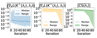
Figure 2: Convergence of Algorithm 1 on 50 randomly sampled problem instances vs iteration $m$.

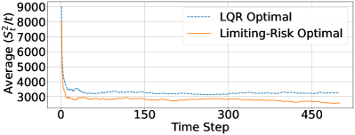
Figure 3: The average running covariance $S_{t}^{2}/t$ over 100 system responses under LQR versus Ergodic-Risk optimal policies.

We also show how the Ergodic-Risk optimal policy behaves compared to the LQR optimal policy. In addition to its resilience to large disturbances observed in [13, 14], here we compare their performance in terms of the running variance of the cumulative risk—which we have now guaranteed to be well-defined. In particular, we consider one of the random problem instances from the previous setup and this time set $\bar{\beta}=0.7\gamma_{N}^{2}(K_{LQR})$. In Figure 3, we illustrate the average of $S_{t}^{2}/t$ with $S_{t}$ defined in equation 4 over 1000 roll-outs of the dynamics in equation 1 with $\mathbb{P}_{W}$ being Student’s t-distribution with parameter $\nu=5$. Note that this noise distribution has finite fourth moment and unbounded fifth moment. Also, recall that $\gamma_{N}^{2}$ is an estimate of $\gamma_{M}^{2}=\lim_{t\to\infty}{\mathbb{E}\,}[S_{t}^{2}/t]$ (Remark 13); therefore, the simulation illustrates that the proposed Ergodic-Risk policy from equation 26 results in smaller (empirical) values, confirming a more risk averse behavior compared to the LQR optimal one.

VI Conclusions

We introduced ergodic-risk criteria in COCP as a flexible framework to capture long-term cumulative uncertainties using appropriate risk functionals. By considering linear constraints on $\gamma_{N}^{2}$ and integrating recent advances in policy optimization, we proposed a primal-dual algorithm with convergence guarantees. A key future direction is extending this approach to directly constrain $\gamma_{M}^{2}$ and develop efficient sample-based algorithms.

References

• [1] R. T. Rockafellar and S. Uryasev, “Optimization of conditional value-at-risk,” The Journal of Risk, vol. 2, no. 3, pp. 21–41, 2000.
• [2] A. Majumdar and M. Pavone, “How Should a Robot Assess Risk? Towards an Axiomatic Theory of Risk in Robotics,” in Robotics Research, pp. 75–84, 2020.
• [3] H.-G. Eichler and B. Bloechl-Daum, et. al., “The risks of risk aversion in drug regulation,” Nature Reviews Drug Discovery, vol. 12, pp. 907–916, Dec. 2013.
• [4] K. Zhang, B. Hu, and T. Başar, “Policy Optimization for H-2 Linear Control with H-infinity Robustness Guarantee: Implicit Regularization and Global Convergence,” SIAM Journal on Control and Optimization, vol. 59, pp. 4081–4109, Jan. 2021.
• [5] P. Whittle, “Risk-Sensitive Linear/Quadratic/Gaussian Control,” Advances in Applied Probability, vol. 13, no. 4, pp. 764–777, 1981.
• [6] V. Borkar and R. Jain, “Risk-Constrained Markov Decision Processes,” IEEE Trans. Autom. Control, pp. 2574–2579, Sept. 2014.
• [7] Y. Chow, M. Ghavamzadeh, L. Janson, and M. Pavone, “Risk-Constrained Reinforcement Learning with Percentile Risk Criteria,” Apr. 2017. arXiv:1512.01629 [cs, math].
• [8] P. Sopasakis, D. Herceg, A. Bemporad, and P. Patrinos, “Risk-averse model predictive control,” Automatica, pp. 281–288, Feb. 2019.
• [9] A. Ruszczyński, “Risk-averse dynamic programming for Markov decision processes,” Math. Program., pp. 235–261, Oct. 2010.
• [10] A. Ahmadi-Javid, “Entropic Value-at-Risk: A New Coherent Risk Measure,” J. Optim. Theory Appl., vol. 155, pp. 1105–1123, Dec. 2012.
• [11] A. Biswas and V. S. Borkar, “Ergodic risk-sensitive control—A survey,” Annual Reviews in Control, vol. 55, pp. 118–141, Jan. 2023.
• [12] M. Kishida and A. Cetinkaya, “Risk-Aware Linear Quadratic Control Using Conditional Value-at-Risk,” IEEE Transactions on Automatic Control, vol. 68, pp. 416–423, Jan. 2023.
• [13] A. Tsiamis, D. S. Kalogerias, L. F. O. Chamon, A. Ribeiro, and G. J. Pappas, “Risk-Constrained Linear-Quadratic Regulators,” Oct. 2020. arXiv:2004.04685 [cs, eess, math].
• [14] F. Zhao and K. You, “Global Convergence of Policy Gradient Primal–Dual Methods for Risk-Constrained LQRs,” IEEE Transactions on Automatic Control, vol. 68, no. 5, 2023.
• [15] S. MEYN and R. L. TWEEDIE, Markov Chains and Stochastic Stability. Cambridge University Press, 2009.
• [16] T. Komorowski and A. Walczuk, “Central limit theorem for Markov processes with spectral gap in the Wasserstein metric,” Stochastic Processes and their Applications, vol. 122, pp. 2155–2184, May 2012.
• [17] S. Talebi, A. Taghvaei, and M. Mesbahi, “Data-driven Optimal Filtering for Linear Systems with Unknown Noise Covariances,” in Advances in Neural Inform. Process. Sys., pp. 69546–69585, 2023.
• [18] S. Talebi and M. Mesbahi, “Policy Optimization over Submanifolds for Linearly Constrained Feedback Synthesis,” IEEE Transactions on Automatic Control, pp. 1–16, 2023.
• [19] S. Meyn, “The policy iteration algorithm for average reward Markov decision processes with general state space,” IEEE Transactions on Automatic Control, vol. 42, pp. 1663–1680, Dec. 1997. Conference Name: IEEE Transactions on Automatic Control.
• [20] P. R. Kumar and P. P. Varaiya, Stochastic systems: estimation, identification, and adaptive control. Classics in applied mathematics, Philadelphia, Pennsylvania: Society for Industrial and Applied Mathematics (SIAM, 3600 Market Street, Floor 6, Philadelphia, PA 19104), 2015. OCLC: 930320873.
• [21] R. Durrett, Probability: Theory and Examples. Cambridge: Cambridge University Press, 5 ed., 2019.
• [22] P. Hall and C. C. Heyde, Martingale Limit Theory and Its Application. Academic Press, Dec. 1980.
• [23] M. Fazel, R. Ge, S. Kakade, and M. Mesbahi, “Global Convergence of Policy Gradient Methods for the Linear Quadratic Regulator,” in Int. Conf. on Machine Learning, pp. 1467–1476, PMLR, July 2018.
• [24] A. Nedić and A. Ozdaglar, “Subgradient Methods for Saddle-Point Problems,” J. Optim. Theory Appl., vol. 142, pp. 205–228, July 2009.