Symmetries of Liouvillians of squeeze-driven parametric oscillators

Abstract

We study the symmetries of the Liouville superoperator of one dimensional parametric oscillators, especially the so-called squeeze-driven Kerr oscillator, and discover a remarkable quasi-spin symmetry $su(2)$ at integer values of the ratio $\eta=\omega/K$ of the detuning parameter $\omega$ to the Kerr coefficient $K$, which reflects the symmetry previously found for the Hamiltonian operator. We find that the Liouvillian of an $su(2)$ representation $\left|j,m_{j}\right\rangle$ has a characteristic double-ellipsoidal structure, and calculate the relaxation time $T_{X}$ for this structure. We then study the phase transitions of the Liouvillian which occur as a function of the parameters $\xi=\varepsilon_{2}/K$ and $\eta=\omega/K$. Finally, we study the temperature dependence of the spectrum of eigenvalues of the Liouvillian. Our findings may have applications in the generation and stabilization of states of interest in quantum computing.

Keywords: open quantum systems, Kerr parametric oscillator, squeeze-driven Kerr oscillator, quasi-spin symmetry, quantum phase transitions, quantum computing

1 Introduction

Symmetries of models in which the Hamiltonian operator is expressed in terms of elements, $\hat{G}_{i}$, of a Lie algebra $g$, appear in many areas of physics, ranging from particle physics [1, 2] to nuclear physics [3] and molecular physics [4]. In these models, $\hat{H}=\sum_{i}\alpha_{i}\hat{G}_{i}$, where $\alpha_{i}$ are tunable parameters, and the algebra $g$ is called the spectrum generating algebra (SGA) of the model. Dynamic symmetries occur when the parameters $\alpha_{i}$ take special values for which $\hat{H}$ becomes a function of the invariant Casimir operators of the algebra $g$. As a result, its eigenvalues can be written in explicit analytic form, making a connection between theory and experiment particularly straightforward. The concept of dynamic symmetry has been so far applied to closed systems. It is of importance to see whether or not this concept can be extended to open quantum systems coupled to an external environment, where the role of the Hamiltonian operator is replaced by that of the Liouvillian superoperator. In this article we address this question and discover a hitherto unknown symmetry of the Liouvillian of one-dimensional parametric oscillators.

In recent years, several parametric models have been considered for possible applications to quantum information science, such as, among others, the Lipkin-Meshkov-Glick model [5], the Kerr oscillator model, the Rabi [6] and Dicke [7] models and the Jaynes-Cummings [8] model. In this article, we concentrate our attention to the squeezed Kerr oscillator, a bosonic model, as a prototype of the class of models comprising, among others, the Lipkin model [5], a fermionic model, and the one-dimensional vibron model [4], a bosonic model. The study of symmetries of models involving coupled systems of bosons and fermions, such as the Rabi, Dicke, and Jaynes-Cummings models, will be deferred to a later publication.

Kerr-nonlinear parametric oscillators (KPOs) can be implemented experimentally with superconducting quantum circuit oscillators, and their applications to quantum computation have been considered by many authors [9, 10, 11, 12, 13, 14, 15, 16, 17, 18, 19, 20]. In a previous publication [21], it was found that the algebraic structure of the Hamiltonian of the squeezed Kerr oscillator

$$\hat{H}=-\omega\hat{a}^{{\dagger}}\hat{a}+K\hat{a}^{{\dagger}2}\hat{a}^{2}-\varepsilon_{2}(\hat{a}^{{\dagger}}\hat{a}^{{\dagger}}+\hat{a}\hat{a})$$ (1)

where $\hat{a}^{{\dagger}},\hat{a}$ are one-dimensional boson creation and annihilation operators satisfying $\left[\hat{a},\hat{a}^{{\dagger}}\right]=1$, is the symplectic algebra $sp(2,\mathcal{R})\sim su(1,1)$. It was also found that, for integer values of the ratio $\omega/K\equiv\eta$ in the Kerr Hamiltonian $\hat{H}=-\omega\hat{a}^{{\dagger}}\hat{a}+K\hat{a}^{{\dagger}2}\hat{a}^{2}$, an unexpected dynamic quasi-spin symmetry, $su(2)$, occurs and that for non-zero values of the ratio $\varepsilon_{2}/K\equiv\xi$ a Quantum Phase Transition (QPT) [22] and an Excited State Quantum Phase Transition (ESQPT) [23, 24, 25] occur [26, 27].

In describing Markovian open quantum systems, one needs to go from a study of the eigenvalues of the Hamiltonian operator to the study of the eigenvalues of the Liouvillian superoperator, which appears in the Lindblad equation and governs dissipative dynamics for the system density matrix [28, 29]. Liouvillians of all parametric oscillators at zero temperature possess $u(1)$ dynamic symmetry, thus eigenvalues can be written in explicit analytic form [30, 31]. However, it turns out that the Liouvillian of the Kerr oscillator also has an unexpected $su(2)$ quasi-spin dynamic symmetry which reflects that found previously for the Hamiltonian operator. We thus extend, in the first part of this paper, the concept of dynamic symmetry from Hamiltonian operators to Liouvillian superoperators. We note that the quasi-spin dynamic symmetry described here is a “local” symmetry in the sense that it occurs only for certain values of the parameters of the model. This symmetry differs from the “global” symmetry $Z_{2}\equiv\Pi$ (parity) [32] of the Liouvillian which occurs for any value in the parameter space.

In the second part of the paper, we study QPTs and ESQPTs of open systems, enlarging the usual definition for closed systems [23]. Our definition for open systems is identical to that proposed in [33], and it considers both the Liouvillian gap [34] and the order parameter. In performing this study we concentrate our attention to the squeeze-driven Kerr oscillator with quadratic squeezing, as a prototype of all squeeze-driven bosonic systems, including the squeeze-driven harmonic oscillator [35] and other squeeze-driven fermionic systems which can be bosonized such as the squeeze-driven Lipkin model [5]. Dissipative phase transitions are of great importance in a variety of fields, including photonic quantum systems [36, 37, 38, 39, 40, 41], and the results presented here can be of use for studying these systems.

Finally, in the third part of the paper, we discuss the effects of a non-zero temperature on the Liouvillian, especially the modification to the eigenvalues of the truncated harmonic oscillator and the Kerr oscillator. In particular, we show that the quasi-spin symmetry $su(2)$ persists even at non-zero temperature, although with modifications. This result is of particular importance in designing quantum hardware, since properties of the Liouvillian determine the relaxation rate of the system.

The key result of this paper is the recognition of the quasi spin-symmetry $su(2)$ of the Liouvillian superoperator, which persists at nonzero squeezing $\xi$ and gives rise to large relaxation times at integer values of the parameter $\eta=\omega/K$. This result is of use for developing quantum computation devices based on the Kerr oscillator (KPO) [9, 10], and generating long-lived states. Another important development is the introduction of algebraic methods to the study of open quantum systems and the derivation in explicit analytic form of solutions for the eigenvalues of the Liouvillian superoperator. The algebraic structure of one-dimensional oscillators is relatively simple, but algebraic methods can play an important role in more complex situations of coupled oscillators, or oscillators in many dimensions, as shown in [3, 4] for applications to nuclear and molecular physics.

This paper is structured as follows. We first introduce the theoretical framework in section 2.1, derive analytic expressions for the eigenvalues of parametric one-dimensional oscillators in sections 2.2 and 2.3, and confirm analytical formulas with numerical calculations in section 2.4. In section 3 we introduce and discuss the $su(2)$ quasispin symmetry of the Kerr oscillator Liouvillian. In section 4, we consider the squeezed Kerr oscillator, and in section 4.1, we discuss the structure of the eigenvalues of the Liouville superoperator. In section 5, we study the QPTs that occur as a function of the parameters $\xi=\varepsilon_{2}/K$ and $\eta=\omega/K$, first for the Hamiltonian in section 5.1, and second for the Liouvillian in section 5.2, for a fixed value of the ratio $\zeta=\kappa/K$ of the dissipator $\kappa$ to the Kerr coefficient $K$. We discuss thermodynamic limits of these QPTs in sections 5.2.1 and 5.2.2. In section 6, we consider temperature dependence, and finally, in section 7, we present our conclusions and indicate directions for future work.

2 Spectral theory of parametric one-dimensional oscillators

2.1 Theoretical framework

Consider an open quantum system with Hilbert space $\mathcal{H}$, Hamiltonian $\hat{H}$, and system density matrix $\hat{\rho}(t)$. Assuming the system obeys Markovian dynamics, it can be described by the Lindblad master equation [28, 29, 42]

$$\partial_{t}\hat{\rho}(t)=-\rmi\left[\hat{H},\hat{\rho}(t)\right]+\sum_{i}\kappa_{i}\mathcal{D}[\hat{\Gamma}_{i}]\hat{\rho}(t),$$ (2)

where $\hat{H}$ is in units of $\hbar$ and the dissipation superoperator $\mathcal{D}[\hat{\Gamma}_{i}]$ is [28, 29, 42]

$$\mathcal{D}\left[\hat{\Gamma}_{i}\right]\hat{\rho}(t)=\hat{\Gamma}_{i}\hat{\rho}(t)\hat{\Gamma}_{i}^{{\dagger}}-\frac{1}{2}\left[\hat{\Gamma}_{i}^{{\dagger}}\hat{\Gamma}_{i}\hat{\rho}(t)+\hat{\rho}(t)\hat{\Gamma}_{i}^{{\dagger}}\hat{\Gamma}_{i}\right]$$ (3)

Here $\hat{\Gamma}_{i}$ is the Lindblad operator associated with a specific dissipation channel occurring at a rate $\kappa_{i}\geq 0$ and describes how the environment acts on the system. Since the Lindblad equation is linear in $\hat{\rho}$, it can be expressed in terms of the so-called Liouville superoperator $\mathcal{L}$

$$\partial_{t}\hat{\rho}(t)=\mathcal{L}\hat{\rho}(t)$$ (4)

which contains an imaginary part describing unitary evolution and a real part characterizing dissipation

$$\mathcal{L}\hat{\rho}(t)=\mathcal{L}^{(0)}\hat{\rho}(t)+\mathcal{L}^{(1)}\hat{\rho}(t)$$ (5)

where

$$\mathcal{L}^{(0)}\hat{\rho}(t)=-\rmi\left[\hat{H},\hat{\rho}(t)\right],\qquad\mathcal{L}^{(1)}\hat{\rho}(t)=\sum_{i}\kappa_{i}\mathcal{D}\left[\hat{\Gamma}_{i}\right]\hat{\rho}(t).$$ (6)

We have denoted here operators by a hat and superoperators (i.e. operators of operators) by a script letter. Superoperators, such as $\mathcal{L}$, acts on the space of linear operators on $\mathcal{H}$, which we will denote as $\mathcal{H}\otimes\mathcal{H}$. The operator space $\mathcal{H}\otimes\mathcal{H}$ is itself a Hilbert space, with inner product between $\hat{A},\hat{B}\in\mathcal{H}\otimes\mathcal{H}$ given by the Hilbert-Schmidt inner product [42],

$$\left\langle\hat{A},\hat{B}\right\rangle=\mathrm{Tr}\left[\hat{A}^{{\dagger}}\hat{B}\right].$$ (7)

The eigenvalues of the Liouvillian $\mathcal{L}$ will be denoted by $\lambda_{i}$

$$\mathcal{L}\hat{\rho}_{i}=\lambda_{i}\hat{\rho}_{i}$$ (8)

where $\hat{\rho}_{i}$ is the eigenmatrix corresponding to eigenvalue $\lambda_{i}$. Note that here we have dropped the time dependence for simplicity. The Liouvillian $\mathcal{L}$ is not Hermitian, so its eigenvalues $\lambda_{i}$ may be complex,

$$\lambda_{i}=\rmi\lambda_{i}^{(0)}+\lambda_{i}^{(1)},$$ (9)

and its eigenmatrices are not necessarily orthogonal,

$$\left\langle\hat{\rho}_{i},\hat{\rho}_{j\neq i}\right\rangle=\mathrm{Tr}\left[\hat{\rho}_{i}^{{\dagger}}\hat{\rho}_{j\neq i}\right]\neq 0$$ (10)

It can be proven [42] that $\mathrm{Re}[\lambda_{i}]\leq 0$ $\forall\lambda_{i}$, and there is always a zero eigenvalue $\lambda_{0}=0$. Moreover, complex eigenvalues occur in conjugate pairs, as (8) implies

$$\mathcal{L}\hat{\rho}_{i}^{{\dagger}}=\lambda_{i}^{\ast}\hat{\rho}_{i}^{{\dagger}}.$$ (11)

Proof: Taking the adjoint of (8) and rewriting in terms of (2) gives

$$\left(\mathcal{L}\hat{\rho}_{i}\right)^{{\dagger}} = \left(-\rmi\left[\hat{H},\hat{\rho}_{i}\right]\right)^{{\dagger}}+\sum_{k}\kappa_{k}\left(\hat{\Gamma}_{k}\hat{\rho}_{i}\hat{\Gamma}_{k}^{{\dagger}}-\frac{1}{2}\left[\hat{\Gamma}_{k}^{{\dagger}}\hat{\Gamma}_{k}\hat{\rho}_{i}+\hat{\rho}_{i}\hat{\Gamma}_{k}^{{\dagger}}\hat{\Gamma}_{k}\right]\right)^{{\dagger}}$$ (12)

$$= -\rmi\left[\hat{H},\hat{\rho}_{i}^{{\dagger}}\right]+\sum_{i}\kappa_{i}\hat{\Gamma}_{k}\hat{\rho}_{i}^{{\dagger}}\hat{\Gamma}_{k}^{{\dagger}}-\frac{1}{2}\left[\hat{\Gamma}_{k}^{{\dagger}}\hat{\Gamma}_{k}\hat{\rho}_{i}^{{\dagger}}+\hat{\rho}_{i}^{{\dagger}}\hat{\Gamma}_{k}^{{\dagger}}\hat{\Gamma}_{k}\right]$$

$$= \mathcal{L}\hat{\rho}_{i}^{{\dagger}}=\lambda_{i}^{\ast}\hat{\rho}_{i}^{{\dagger}}.$$

Eigenmatrices $\hat{\rho}_{i}$ need not be Hermitian, and if $\hat{\rho}_{i}$ is Hermitian, the eigenvalue $\lambda_{i}=\lambda_{i}^{\ast}$ must be real. Consequently, real eigenvalues of degeneracy 1 must have corresponding Hermitian eigenmatrices $\hat{\rho}_{i}$, and it is always possible to construct Hermitian linear combinations of eigenmatrices for degenerate real eigenvalues $\lambda_{i}$ of the form $\left(\hat{\rho}_{i}+\hat{\rho}_{i}^{{\dagger}}\right)$ and $\rmi\left(\hat{\rho}_{i}-\hat{\rho}_{i}^{{\dagger}}\right)$.

For computational purposes, it is convenient to work with a vectorized representation of operators and a matrix representation of superoperators [17, 18, 32, 33, 43], where, given a basis $\left\{\left|e_{n}\right\rangle\right\}$ of $\mathcal{H}$, an operator $\hat{A}\in\mathcal{H}\otimes\mathcal{H}$ is mapped to a vector

$$\hat{A}=\sum_{n,m}A_{nm}\left|e_{n}\right\rangle\left\langle e_{m}\right|\rightarrow\left|A\right\rangle\rangle=\sum_{n,m}A_{nm}\left|e_{n}\right\rangle\otimes\left|e_{m}\right\rangle.$$ (13)

From this one can show that left and right multiplication of an operator $\hat{O}\in\mathcal{H}\otimes\mathcal{H}$ on $\hat{A}$ are represented by matrix superoperators as

$$\hat{O}\hat{A}\rightarrow\left(\hat{O}\otimes\hat{I}\right)\left|A\right\rangle\rangle,\qquad\hat{A}\hat{O}\rightarrow\left(\hat{I}\otimes\hat{O}^{T}\right)\left|A\right\rangle\rangle,$$ (14)

where $\hat{I}$ is the identity. Applying this mapping to the Liouvillian $\mathcal{L}$ yields

$$\mathcal{L} \rightarrow -\rmi\left[\left(\hat{H}\otimes\hat{I}\right)-\left(\hat{I}\otimes\hat{H}^{T}\right)\right]$$ (15)

$$+\sum_{i}\kappa_{i}\left[\left(\hat{\Gamma}_{i}\otimes\hat{\Gamma}_{i}^{\ast}\right)-\frac{1}{2}\left(\hat{\Gamma}_{i}^{{\dagger}}\hat{\Gamma}_{i}\otimes\hat{I}\right)-\frac{1}{2}\left(\hat{I}\otimes\hat{\Gamma}_{i}^{T}\hat{\Gamma}_{i}^{\ast}\right)\right].$$

It is important to note that eigenmatrices of the Liouvillian are not density matrices, since to be a physical density matrix, $\hat{\rho}(t)$ must be Hermitian, positive definite, and have unit trace. However, it is possible [33] to construct density matrices from Hermitian linear combinations of eigenmatrices $\hat{\rho}_{i}$.

2.2 Spectral theory of one-dimensional oscillators

We consider here one-dimensional oscillators with Hamiltonian written in terms of one-dimensional creation and annihilation operators $\hat{a}^{{\dagger}},\hat{a}$ with commutation relation $\left[\hat{a},\hat{a}^{{\dagger}}\right]=1$,

$$\hat{H}=\omega_{1}(\hat{a}^{{\dagger}}\hat{a})+\omega_{2}(\hat{a}^{{\dagger}}\hat{a})^{2}+\omega_{3}(\hat{a}^{{\dagger}}\hat{a})^{3}+...=\sum_{k}\omega_{k}(\hat{a}^{{\dagger}}\hat{a})^{k},$$ (16)

where $\omega_{k}$ are tunable parameters. The eigenvalues of $\hat{H}$ are trivially given by

$$E_{n}=\omega_{1}n+\omega_{2}n^{2}+\omega_{3}n^{3}+...,\qquad n=0,1,2,...$$ (17)

and the eigenfunctions by

$$\left|n\right\rangle=\frac{1}{\sqrt{n!}}(\hat{a}^{{\dagger}})^{n}\left|0\right\rangle.$$ (18)

The Hilbert space $\mathcal{H}$ of this oscillator is infinite-dimensional, but may be truncated in practical applications to a finite number of bosonic excitations $N$, such that $n=0,1,...,N$. The model Hilbert space $\mathcal{H}$ of this truncated oscillator is of dimension $N_{\rm Fock}=N+1$, and is an invariant subspace of the untruncated, infinite-dimensional space.

The most general spectrum generating algebra for one-dimensional oscillators is the Heisenberg algebra $h(2)$ [31], composed of operators $\hat{a},\hat{a}^{{\dagger}},\hat{a}^{{\dagger}}\hat{a}$, and the identity operator $\hat{I}$, with commutation relations

$$\left[\hat{a},\hat{a}^{{\dagger}}\right] = \hat{I},\quad\left[\hat{a},\hat{I}\right]=\left[\hat{a}^{{\dagger}},\hat{I}\right]=0$$

$$\left[\hat{a},\hat{a}^{{\dagger}}\hat{a}\right] = \hat{a},\quad\left[\hat{a}^{{\dagger}},\hat{a}^{{\dagger}}\hat{a}\right]=-\hat{a}^{{\dagger}}.$$ (19)

$h(2)$ is non-compact and its representations are infinite-dimensional. To perform calculations for truncated oscillators with finite $N$, it is convenient to introduce an auxiliary boson $s$ [31] and introduce operators $\hat{F}_{-}=\hat{s}^{{\dagger}}\hat{a}$, $\hat{F}_{+}=\hat{a}^{{\dagger}}s$, $\hat{n}=\hat{a}^{{\dagger}}\hat{a}$, $\hat{n}_{s}=\hat{s}^{{\dagger}}\hat{s}$, such that $\hat{n}+\hat{n}_{s}=\hat{N}$ gives the total boson number $N$. These four operators satisfy the Lie algebra of $u(2)$, which is therefore a spectrum generating algebra for the truncated oscillator. By considering only $\hat{n}=\hat{a}^{{\dagger}}\hat{a}$, one has the algebra of $u(1)$, a subalgebra of $u(2)$ and $h(2)$, often written as $u(2)\supset u(1)$ or $h(2)\supset u(1)$. Formally, one may obtain the algebra $h(2)$ from $u(2)$ by replacing the operators $\hat{s}$ and $\hat{s}^{{\dagger}}$ by $\sqrt{N}$ and taking the limit $N\rightarrow\infty$. The algebra $h(2)$ is called the contracted algebra of $u(2)$ and denoted by

$$u(2)\rightarrow_{c}h(2).$$ (20)

The Hamiltonian $\hat{H}$ in (16) is written in terms only of the $u(1)$ Casimir operator, $\hat{n}=\hat{a}^{{\dagger}}\hat{a}$, and thus has a so-called $u(1)$ “dynamic symmetry”, that is, a situation in which $\hat{H}$ is written in terms only of invariant operators of an algebra. Note that although for one-dimensional problems this is a trivial statement, it is not so for higher dimensional problems as described in [31].

For the open system, we consider bosonic dissipators

$$\mathcal{D}\left[\hat{a}^{k}\right]\hat{\rho}(t)=\hat{a}^{k}\hat{\rho}(t)\hat{a}^{{\dagger}k}-\frac{1}{2}\left[\hat{a}^{{\dagger}k}\hat{a}^{k}\hat{\rho}(t)+\hat{\rho}(t)\hat{a}^{{\dagger}k}\hat{a}^{k}\right].$$ (21)

Particularly important are the linear

$$\mathcal{D}\left[\hat{a}\right]\hat{\rho}(t)=\hat{a}\hat{\rho}(t)\hat{a}^{{\dagger}}-\frac{1}{2}\left[\hat{a}^{{\dagger}}\hat{a}\hat{\rho}(t)+\hat{\rho}(t)\hat{a}^{{\dagger}}\hat{a}\right]$$ (22)

and quadratic

$$\mathcal{D}\left[\hat{a}^{2}\right]\hat{\rho}(t)=\hat{a}^{2}\hat{\rho}(t)\hat{a}^{{\dagger}2}-\frac{1}{2}\left[\hat{a}^{{\dagger}2}\hat{a}^{2}\hat{\rho}(t)+\hat{\rho}(t)\hat{a}^{{\dagger}2}\hat{a}^{2}\right]$$ (23)

dissipators, which may describe one- and two-photon losses to the environment [17, 18, 19]. We note here that the dissipators are also built in terms of elements of $h(2)$ and their powers. The powers of algebra elements also form an algebra, called the enveloping algebra of $h(2)$. However, one only needs the representation theory of $h(2)$ to make use of its enveloping algebra in calculations.

In order to find the eigenvalues of $\mathcal{L}$ for these models, one must construct a basis for its eigenmatrices $\hat{\rho}_{i}$. A generic operator for a one-dimensional bosonic system can be expanded onto a Fock basis $\left\{\left|n\right\rangle\right\}$ of oscillator eigenfunctions,

$$\hat{\rho}=\sum_{n,m}\rho_{nm}\left|n\right\rangle\left\langle m\right|$$ (24)

where $\rho_{nm}$ are its matrix elements, and we have dropped the time dependence of $\rho_{nm}$ for simplicity. $\hat{\rho}$ is an element of the operator Hilbert space $\mathcal{H}\otimes\mathcal{H}$, which for the truncated oscillator, has dimension $(N+1)\times(N+1)=N_{\rm Fock}\times N_{\rm Fock}$.

When there is a $u(1)$ dynamic symmetry, the Hamiltonian is diagonal in the basis $\left\{\left|n\right\rangle\right\}$, with eigenvalues $E_{n}$. Hence, the imaginary part of the Liouvillian $\mathcal{L}^{(0)}\hat{\rho}=-\rmi\left[\hat{H},\hat{\rho}\right]$ is also diagonal, as one can see by expanding $\left[\hat{H},\hat{\rho}\right]=\hat{H}\hat{\rho}-\hat{\rho}\hat{H}$ and using $\hat{\rho}$ from (24). Thus, $\mathcal{L}^{(0)}$ has eigenmatrices of the form $\left|n\right\rangle\left\langle m\right|$ and spectrum given by

$$\mathcal{L}^{(0)}\left|n\right\rangle\left\langle m\right|=-\rmi(E_{n}-E_{m})\left|n\right\rangle\left\langle m\right|.$$ (25)

We remark that $\mathcal{L}^{(0)}$ simply describes the closed system with no dissipation. Introducing linear dissipation with strength $\kappa$, the Liouvillian at zero temperature is $\mathcal{L}=\mathcal{L}^{(0)}+\mathcal{L}^{(1)}$, with dissipator

$$\mathcal{L}^{(1)}\hat{\rho}=\kappa\left(\hat{a}\hat{\rho}\hat{a}^{{\dagger}}-\frac{1}{2}(\hat{a}^{{\dagger}}\hat{a}\hat{\rho}+\hat{\rho}\hat{a}^{{\dagger}}\hat{a})\right).$$ (26)

In the Fock basis, we find the Liouvillian, $\mathcal{L}=\mathcal{L}^{(0)}+\mathcal{L}^{(1)}$, has matrix elements given by

$$\mathcal{L}\left|n\right\rangle\left\langle m\right| = \left[-\rmi\left(E_{n}-E_{m}\right)-\frac{\kappa}{2}(n+m)\right]\left|n\right\rangle\left\langle m\right|$$ (27)

$$+\left[\kappa\sqrt{n}\sqrt{m}\right]\left|n-1\right\rangle\left\langle m-1\right|$$

Making use of the vectorized representation (13), we note that the matrix representative of $\mathcal{L}$ is upper triangular in the Fock basis,

$$\left(\matrix{\lambda_{00}&\times&&\cr&\lambda_{01}&\times&\cr&&\lambda_{02}&\times\cr 0&&&\ddots}\right)$$ (28)

with eigenvalues given by its diagonal elements, which are therefore

$$\lambda_{n,m}=-\rmi\left(E_{n}-E_{m}\right)-\frac{\kappa}{2}(n+m).$$ (29)

Note that the real part of $\lambda_{n,m}$ is always $<0$ and there is a zero eigenvalue $n=m=0$. Also, eigenmatrices $\hat{\rho}_{n,m}\neq\left|n\right\rangle\left\langle m\right|$ due to off-diagonal matrix elements of $\mathcal{L}$, however, we are not concerned with explicit expressions of $\hat{\rho}_{n,m}$ here.

As another example, one can treat the Liouvillian at zero-temperature with quadratic dissipation similarly, $\mathcal{L}=\mathcal{L}^{(0)}+\mathcal{L}^{(1)}$, where

$$\mathcal{L}^{(1)}\hat{\rho}=\kappa_{2}\left(\hat{a}^{2}\hat{\rho}\hat{a}^{{\dagger}2}-\frac{1}{2}(\hat{a}^{{\dagger}2}\hat{a}^{2}\hat{\rho}+\hat{\rho}\hat{a}^{{\dagger}2}\hat{a}^{2})\right)$$ (30)

and $\kappa_{2}$ is the strength of dissipation. Following the same treatment as above for linear dissipation, the Liouvillian has Fock basis matrix elements

$$\mathcal{L}\left|n\right\rangle\left\langle m\right| = \left[-\rmi\left(E_{n}-E_{m}\right)-\frac{\kappa_{2}}{2}\left(n(n-1)+m(m-1)\right)\right]\left|n\right\rangle\left\langle m\right|$$ (31)

$$+\left[\kappa_{2}\sqrt{n(n-1)}\sqrt{m(m-1)}\right]\left|n-2\right\rangle\left\langle m-2\right|$$

and eigenvalues

$$\lambda_{n,m}=-\rmi\left(E_{n}-E_{m}\right)-\frac{\kappa_{2}}{2}\left[n(n-1)+m(m-1)\right]$$ (32)

In principle one may follow this procedure for linear combinations of dissipators of arbitrary $k$-photon losses, (21), but in this article we will focus on the linear case.

In section 6 we will also consider non-zero temperatures parametrized in terms of an average thermal population $\bar{n}_{\rm th}$. The linear dissipator at non-zero temperature is [17, 18, 19]

$$\mathcal{L}^{(1)}\hat{\rho}=\kappa\left(1+\bar{n}_{\rm th}\right)\mathcal{D}\left[\hat{a}\right]\hat{\rho}+\kappa\bar{n}_{\rm th}\mathcal{D}\left[\hat{a}^{{\dagger}}\right]\hat{\rho}.$$ (33)

The new term here is

$$\mathcal{D}\left[\hat{a}^{{\dagger}}\right] = \hat{a}^{{\dagger}}\hat{\rho}\hat{a}-\frac{1}{2}\left(\hat{a}\hat{a}^{{\dagger}}\hat{\rho}+\hat{\rho}\hat{a}\hat{a}^{{\dagger}}\right)$$ (34)

$$= \hat{a}^{{\dagger}}\hat{\rho}\hat{a}-\frac{1}{2}\left[\left(1+\hat{a}^{{\dagger}}\hat{a}\right)\hat{\rho}+\hat{\rho}\left(1+\hat{a}^{{\dagger}}\hat{a}\right)\right].$$

The combined linear dissipator at non-zero temperature, can then be written as

$$\mathcal{L}^{(1)}\hat{\rho} = \kappa\left(\hat{a}\hat{\rho}\hat{a}^{{\dagger}}-\frac{1}{2}\left(\hat{a}^{{\dagger}}\hat{a}\hat{\rho}+\hat{\rho}\hat{a}^{{\dagger}}\hat{a}\right)\right)$$ (35)

$$+\kappa\bar{n}_{\rm th}\left(\hat{a}\hat{\rho}\hat{a}^{{\dagger}}+\hat{a}^{{\dagger}}\hat{\rho}\hat{a}\right)-\kappa\bar{n}_{\rm th}\left(\hat{a}^{{\dagger}}\hat{a}\hat{\rho}+\hat{\rho}\hat{a}^{{\dagger}}\hat{a}+\hat{\rho}\right).$$

The full Liouvillian, $\mathcal{L}=\mathcal{L}^{(0)}+\mathcal{L}^{(1)}$, has matrix elements

$$\mathcal{L}\left|n\right\rangle\left\langle m\right| = \left[-\rmi\left(E_{n}-E_{m}\right)-\frac{\kappa}{2}(1+2\bar{n}_{\rm th})(n+m)-\kappa\bar{n}_{\rm th}\right]\left|n\right\rangle\left\langle m\right|$$ (36)

$$+\left[\kappa(1+\bar{n}_{\rm th})\sqrt{n}\sqrt{m}\right]\left|n-1\right\rangle\left\langle m-1\right|$$

$$+\left[\kappa\bar{n}_{\rm th}\sqrt{n+1}\sqrt{m+1}\right]\left|n+1\right\rangle\left\langle m+1\right|$$

The matrix representative of $\mathcal{L}$ is now tridiagonal,

$$\left(\matrix{L_{00}&\times&&\cr\times&L_{11}&\times&\cr&\times&L_{12}&\times\cr&&\times&\ddots}\right)$$ (37)

and has eigenvalues which generally must be computed numerically.

2.3 Specific cases at zero temperature

In the following sections, our analysis will focus on the zero temperature case, $\bar{n}_{\rm th}=0$, for simplicity and clarity. We will consider non-zero temperatures, $\bar{n}_{\rm th}\neq 0$, in section 6.

2.3.1 Harmonic oscillator.

The algebraic Hamiltonian is

$$\hat{H}=\omega\left(\hat{a}^{{\dagger}}\hat{a}\right)=\omega\hat{n}$$ (38)

with eigenvalues

$$E_{n}=\omega n$$ (39)

The eigenvalues of the Liouvillian superoperator are

$$\lambda_{n,m}=-\rmi\omega\left(n-m\right)-\frac{\kappa}{2}(n+m).$$ (40)

2.3.2 Kerr oscillator.

The Kerr oscillator has gained recent attention for its potential applications to quantum computing [10, 17, 18]. Its algebraic Hamiltonian is

$$\hat{H}=-\omega\hat{a}^{{\dagger}}\hat{a}+K\hat{a}^{{\dagger}2}\hat{a}^{2}=-\omega\hat{n}+K\hat{n}(\hat{n}-1)$$ (41)

with eigenvalues

$$E_{n}=-\omega n+Kn(n-1).$$ (42)

The parameter $\omega$ is denoted by $\Delta$ in [17, 18]. It is convenient to introduce a dimensionless Hamiltonian

$$\frac{\hat{H}}{K}=-\frac{\omega}{K}\hat{n}+\hat{n}(\hat{n}-1)=-\eta\hat{n}+\hat{n}(\hat{n}-1)=-\eta^{\prime}\hat{n}+\hat{n}^{2}.$$ (43)

with eigenvalues

$$E_{n}=-\eta^{\prime}n+n^{2}.$$ (44)

The eigenvalues of the Liouvillian of the Kerr oscillator are

$$\lambda_{n,m}=-\rmi\left[\left(-\eta^{\prime}n+n^{2}\right)-\left(-\eta^{\prime}m+m^{2}\right)\right]-\frac{\kappa}{2}(n+m).$$ (45)

The Hamiltonian of the Kerr oscillator has a quasi-spin symmetry for integer values of the parameter $\eta^{\prime}=\eta+1$ [21] which will be reflected into symmetries of the eigenvalues of the Liouvillian superoperator to be discussed in the following subsections.

2.4 Numerical evaluation of the eigenvalues

In order to evaluate numerically the eigenvalues of the Liouville superoperator, one must use the vectorized representation (13-15) and diagonalize $\mathcal{L}$ in a truncated $N_{\rm Fock}\times N_{\rm Fock}$ dimensional space. Diagonalization gives complex eigenvalues

$$\lambda_{i}=\mathrm{Re}[\lambda_{i}]+\rmi\cdot\mathrm{Im}[\lambda_{i}].$$ (46)

which can be displayed as a scatterplot in the complex plane. We consider here the harmonic oscillator (38) and the Kerr oscillator (41) with linear dissipation. In all subsequent figures we use a strength of dissipation $\kappa=0.1$ and $N_{\rm Fock}=10$.

2.4.1 Harmonic oscillator.

The Liouvillian spectrum for $\omega=-1,K=0$ is shown in figure 1.

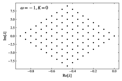
Figure 1: Scatterplot of the harmonic oscillator ($\omega=-1,K=0$) Liouvillian eigenvalues in the complex plane for $N_{\rm Fock}=10$.

The scatterplot of the harmonic oscillator eigenvalues has two symmetries, reflection symmetry about the real axis $n\leftrightarrow m$, and reflection about the imaginary axis at $-\kappa\frac{N}{2}=-\kappa\frac{N_{\rm Fock}-1}{2}$. While the former occurs for any size of the Hilbert space $\mathcal{H}$ due to eigenvalues occurring in conjugate pairs (11), the latter depends on the size $N_{\rm Fock}=N+1$ of the Hilbert space.

As discussed in subsection 2.2, the algebraic structure of the harmonic oscillator for finite $N$ is $u(2)\supset u(1)$. Bosonic representations of $u(2)$ are totally symmetric representations characterized by the integer $N$, while those of $u(1)$ are characterized by the integer $n$, with $n=0,1,2,...,N$, written symbolically as [31]

$$\left|\begin{array}[]{ccc}\vspace{-0.2em}u(2)&\supset&u(1)\\ \vspace{-0.2em}\downarrow&&\downarrow\\ [N]&&n\end{array}\right\rangle,\qquad n=0,1,2,...,N.$$ (47)

Numerical diagonalization confirms the analytic formula (40) obtained by using the dynamic symmetry of the harmonic oscillator. From (40) one can also see that the geometric reflection symmetry of the scatterplot about the imaginary axis changes $n,m$ into $n\rightarrow N-m,m\rightarrow N-n$.

2.4.2 Kerr oscillator.

Liouvillian spectrum scatterplots for $\omega=-1,0,1,2,3,4$ , $K=1$ for $N_{\rm Fock}=10$ are shown in figure 2, and agree with the analytic formula (45).

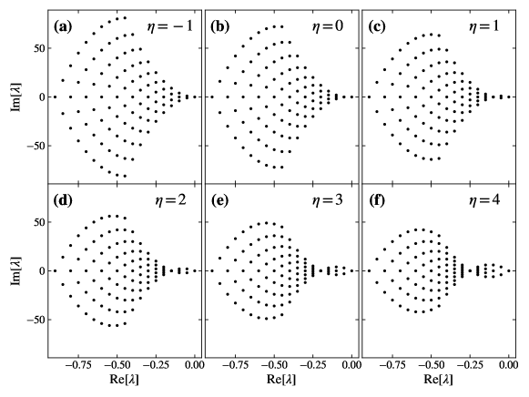
Figure 2: Scatterplots of the Kerr oscillator Liouvillian spectrum for integer values of the ratio $\omega/K=\eta=-1,0,1,2,3,4$ for $N_{\rm Fock}=10$.

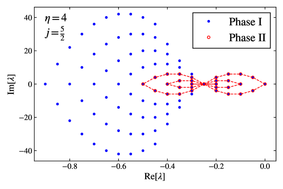
Figure 3: Scatterplot of the Kerr oscillator Liouvillian spectrum for $\omega/K=\eta=4$ showing the separation of eigenvalues into two phases, Phase I (blue) and Phase II (red).

The eigenvalues of the Hamiltonian of the Kerr oscillator have a two phase structure [21]. In Phase I states are singly degenerate, while in Phase II they are doubly degenerate. It has been found that Phase II has, for integer values of $\eta$, a remarkable quasi-spin $su(2)$ symmetry, with states characterized by quasi-spin representations $\left|j,m_{j}\right\rangle$, with $j=\frac{\eta+1}{2}$ and energies counted from the lowest state given by $E-E_{\rm min}=m_{j}^{2}$ for integer $j$ and $E-E_{\rm min}=m_{j}^{2}-\frac{1}{4}$ for half integer $j$ [21]. This quasi-spin symmetry $su(2)$ is not the same as the symmetry of the one-dimensional harmonic oscillator discussed in subsection 2.2, and it represents a major novel finding. Details of the derivation of the quasi-spin symmetry $su(2)$, its construction using two boson operators, and its role in determining the eigenvalues of the Hamiltonian $\hat{H}$ are given in [21] and A. It is a remarkable result of the present article that both the two phase structure and the $su(2)$ quasi-spin symmetry appear in the eigenvalues of the Liouville superoperator. The eigenvalues of $\mathcal{L}$ for Phase I have the same structure of the anharmonic oscillator, $\omega=-1,K=1$ (figure 2a). The eigenvalues of $\mathcal{L}$ for Phase II have a characteristic double-ellipsoidal structure which is different for $\eta=\mathrm{even}$ and $\eta=\mathrm{odd}$, and a highly degenerate accumulation point. The two structures are interpenetrating, as shown for $\eta=\omega/K=4$ in figure 3, where the two structures are color coded, Phase I in blue and Phase II in red. Note that the accumulation point at the center of the double-ellipsoidal structure of Phase II is six-fold degenerate.

3 Quasi-spin symmetry of the Kerr oscillator Liouvillian

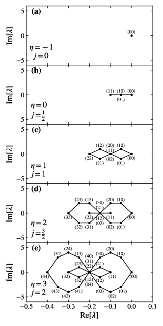
Figure 4: Eigenvalues of the Liouvillian superoperator of the Kerr oscillator for irreducible representations $\left|j,m_{j}\right\rangle$ of $su(2)_{j}$ with $j=0,1/2,1,3/2,2$. Points are labeled by $(n,m)=\left(j-m_{j},j-m_{j}^{\prime}\right)$, (45). Note the accumulation point at the center of the double-ellispoidal structure.

The $su(2)$ quasi-spin symmetry of the Kerr oscillator Liouvillian appears as a consequence of the Hamiltonian symmetry. As discussed in A, the Hamiltonian projected onto the Phase II subspace of the Kerr oscillator can be written in quasi-spin notation as

$$\frac{\hat{H}}{K}=\hat{j}_{z}^{2}-\frac{1}{8}\left(1-(-1)^{2j}\right),$$ (48)

acting on states $\left|j,m_{j}\right\rangle$ where $\hat{j}_{z}\left|j,m_{j}\right\rangle=m_{j}\left|j,m_{j}\right\rangle$. Similarly making use of the two-boson construction of representations of $su(2)$ described in A, one can characterize the eigenvalues of the Liouvillian for Phase II in terms of an $su(2)$ representation $\left|j,m_{j}\right\rangle$ $\left(j=\frac{\eta^{\prime}}{2}=\frac{N}{2}\right)$ and its dual representation $j^{\ast}$ (which for $su(2)$ is isomorphic to the original representation $j$ [31]). Eigenvalues, as shown in figure 4, can then be labeled by $(m_{j},m_{j}^{\prime})$ and (45) can be rewritten as

$$\lambda_{j,m_{j},m_{j}^{\prime}}=-\rmi\left(m_{j}^{2}-m_{j}^{\prime 2}\right)-\kappa\left(j-\frac{m_{j}+m_{j}^{\prime}}{2}\right)$$ (49)

where $n=(j-m_{j})$ and $m=(j-m_{j}^{\prime})$. Associated eigenmatrices are denoted $\hat{\rho}_{j,m_{j},m_{j}^{\prime}}$. Furthermore, we can express the Liouvillian $\mathcal{L}$ projected onto the Phase II subspace in terms of quasi-spin operators,

$$\mathcal{L}\hat{\rho}=-\rmi\left[\hat{j}_{z}^{2}-\frac{1}{8}\left(1-(-1)^{2j}\right),\hat{\rho}\right]-\frac{\kappa}{2}\left((j-\hat{j}_{z})\hat{\rho}+\hat{\rho}(j-\hat{j}_{z})\right)$$ (50)

The quasi-spin dynamic symmetry of the Liouvillian is evident here, as $\mathcal{L}$ consists exclusively of invariant operators of $su(2)_{j}$ acting on $\hat{\rho}$ from the left, and invariant operators of the dual $su(2)_{j^{\ast}}$ acting on $\hat{\rho}$ from the right. It is important to clarify that eigenmatrices of $\mathcal{L}$ in the Phase II subspace, $\hat{\rho}_{j,m_{j},m_{j}^{\prime}}$, are not the same as outer products of Hamiltonian eigenstates, $\left|j,m_{j}\right\rangle\left\langle j,m_{j}^{\prime}\right|$, as discussed in subsection 2.2. Rather, the notation $(m_{j},m_{j}^{\prime})$ simply labels Liouvillian eigenmatrices with $su(2)_{j}$ quantum numbers.

From a mathematical point of view, it is interesting to display the eigenvalues of the Liouville superoperator for irreducible representations of $su(2)_{j}$, as shown in figure 4. The symmetries of the Liouvillian are particularly evident in this figure. In addition to the reflection on the $\mathrm{Re}[\lambda]$ axis due to the definition of the Liouvillian (6), there is a symmetry of reflection on the $\mathrm{Im}[\lambda]$ axis at $\mathrm{Re}[\lambda]=-\kappa j$ ($\kappa=0.1$ in the figure). This symmetry is a consequence of the degeneracy of the Hamiltonian, and allows points to the left and to the right of the accumulation point $\mathrm{Re}[\lambda]=-\kappa j$ to be classified separately in conjugate pairs of $su(2)$ representations. To be specific, points to the right of the accumulation point can be classified as representations of $su(2)$, $\left|J,M\right\rangle$ with $0\leq J\leq j$. Points to the left can be classified in a similar way as $\left|\bar{J},\bar{M}\right\rangle$, where $\left|\bar{J},\bar{M}\right\rangle$ are conjugate representations of $su(2)$ obtained from $\left|J,M\right\rangle$ by reflection. These $su(2)$ representations are obtained from the $(m_{j},m_{j}^{\prime})$ or the $(n,m)$ classification by

$$J = j-\frac{m_{j}+m_{j}^{\prime}}{2}=\frac{n+m}{2}$$

$$M = \frac{m_{j}^{\prime}-m_{j}}{2}=\frac{n-m}{2}$$

$$\bar{J} = j+\frac{m_{j}+m_{j}^{\prime}}{2}=(\eta+1)-\frac{n+m}{2}$$

$$\bar{M} = \frac{m_{j}-m_{j}^{\prime}}{2}=-\frac{n-m}{2}$$ (51)

As an example of this classification, the accumulation point at the center of the double-ellipsoidal structure in figure 4e, $\eta=3,j=2$, has $(n,m)=(40),(31),(22),(13),(04)$, forming a representation [31] $J=2$ and $M=\pm 2,\pm 1,0$. In this figure starting from the right and moving to the left, one has $su(2)$ representations grouped in vertical bands $J=0,\frac{1}{2},1,\frac{3}{2}$; $J=\bar{J}=2$; $\bar{J}=\frac{3}{2},1,\frac{1}{2},0$.

The spectrum of the Liouvillian in Phase II can also be expressed in terms of $\left|J,M\right\rangle$ and $\left|\bar{J},\bar{M}\right\rangle$ representations, where, denoting eigenmatrices $\hat{\rho}_{j,J,M}$ and $\hat{\rho}_{j,\bar{J},\bar{M}}$, one obtains

$$\mathcal{L}\hat{\rho}_{j,J,M} =\left[4\rmi\left(j-J\right)M-\kappa J\right]\hat{\rho}_{j,J,M} \qquad 0\leq J\leq j$$

$$\mathcal{L}\hat{\rho}_{j,\bar{J},\bar{M}} =\left[4\rmi\left(j-\bar{J}\right)\bar{M}-\kappa\left(2j-\bar{J}\right)\right]\hat{\rho}_{j,\bar{J},\bar{M}} \qquad 0\leq\bar{J}\leq j$$ (52)

Note that $J=j$ and $\bar{J}=j$ denote the same representation, so one must be careful not to overcount here. All three different forms, $(n,m)$, $(m_{j},m_{j}^{\prime})$, $(J,M)(\bar{J},\bar{M})$, are equivalent and can be obtained from each other by the relation given above.

Particularly interesting is the Liouvillian of a spinor, $j=\frac{1}{2}$, consisting of a line, since the two Hamiltonian eigenstates $n=0$ and $n=1$ are degenerate and therefore $\mathrm{Im}[\lambda]=0$. These degenerate spinor states may be used to form a basis for a qubit.

We note that numerical diagonalization confirms the analytic formulas derived above, and that the $su(2)$ symmetry of the Liouville superoperator at integer values of the parameter $\eta$ has key implications for the stabilization of long-lived states, as will shown be in section 4.

4 Spectral theory of one-dimensional squeezed oscillators

One-dimensional squeezed oscillators have Hamiltonians of the form

$$\hat{H}=\sum_{k}\omega_{k}\left(\hat{a}^{{\dagger}}\hat{a}\right)^{k}+\sum_{k_{\rm s}}\varepsilon_{k_{\rm s}}\left(\hat{a}^{{\dagger}k_{\rm s}}+\hat{a}^{k_{\rm s}}\right)$$ (53)

where $k_{\rm s}$ denotes the order of the squeezing, and zero-temperature linear dissipators $\mathcal{D}[\hat{a}]\hat{\rho}(t)$ given in (22). The eigenvalues of the Liouville superoperator for squeezed oscillators cannot be solved analytically even at zero-temperature. $\hat{H}$ still has a $h(2)$ spectrum generating algebra but no longer has $u(1)$ symmetry. Therefore, its eigenfunctions are of the form

$$\left|\psi_{\alpha}\right\rangle=\sum_{n=0}^{\infty}c_{n}^{(\alpha)}\left|n\right\rangle$$ (54)

and we can no longer use the $u(1)$ symmetry to diagonalize $\mathcal{L}$ as was done in the previous section. In this case, the eigenvalues must be evaluated numerically in a truncated Hilbert space of dimension $N_{\rm Fock}=N+1$. The dimension of the Hilbert space plays here an important role especially for large values of the parameters $\varepsilon_{k_{\rm s}}$, since the truncated space is invariant under the action of $\hat{a}^{{\dagger}}\hat{a}$ and $\hat{a}$, but not of $\hat{a}^{{\dagger}}$. Thus, careful attention must be given to $N_{\rm Fock}$ to ensure convergence of eigenvalues and properties of interest.

In this article, we consider squeezed Kerr oscillators with linear dissipation, the class of models with Hamiltonian $\hat{H}$ and Liouvillian $\mathcal{L}=\mathcal{L}^{(0)}+\mathcal{L}^{(1)}$ given by

$$\hat{H} = -\omega\hat{a}^{{\dagger}}\hat{a}+K\hat{a}^{{\dagger}2}\hat{a}^{2}-\varepsilon_{2}\left(\hat{a}^{{\dagger}2}+\hat{a}^{2}\right)$$

$$\mathcal{L}^{(1)}\hat{\rho} = \kappa\left(\hat{a}\hat{\rho}\hat{a}^{{\dagger}}-\frac{1}{2}(\hat{a}^{{\dagger}}\hat{a}\hat{\rho}+\hat{\rho}\hat{a}^{{\dagger}}\hat{a}\right).$$ (55)

These models have been proposed as devices for robust quantum computation [10] and squeezing can be implemented experimentally with superconducting circuits [17, 18, 19].

4.1 Evolution of the Liouvillian eigenvalues as a function of $\varepsilon_{2}/K$

We have studied numerically the eigenvalues of the Liouville superoperator for the harmonic oscillator and the squeezed Kerr oscillator as a function of the parameter $\varepsilon_{2}$. In all scatterplots shown below we have used $\kappa=0.1$.

4.1.1 Squeezed Harmonic oscillator.

The Liouvillian spectrum for $\omega=-1,K=0$ is shown in figure 5 as a function of squeezing $\varepsilon_{2}$. Here, squeezing leads to the formation of structures similar to those of figure 4. At $\varepsilon_{2}=1.0$, one can recognize a representation $j^{\prime}=1/2$ of $su(2)$ consisting of a line with four points (see figure 4) with $-0.2\leq\mathrm{Re}[\lambda]\leq 0$. We denote these representations $\left|j^{\prime},m^{\prime}\right\rangle$ since they are different from the representations $\left|j,m_{j}\right\rangle$ discussed previously.

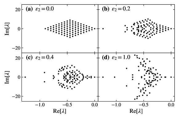
Figure 5: Scatterplot of the squeezed harmonic oscillator ($\omega=-1,K=0$) Liouvillian spectrum for $\varepsilon_{2}=0,0.2,0.4,1.0$, and $N_{\rm Fock}=10$.

4.1.2 Squeezed Kerr oscillator.

We have investigated the Liouvillian spectrum of the squeezed Kerr oscillator for $\omega=-1,0,1$, $K=1$. The dimensionless Hamiltonian for these cases is

$$\frac{\hat{H}}{K}=-\eta\hat{n}+\hat{n}(\hat{n}-1)-\xi\hat{P}_{2}$$ (56)

where $\hat{n}=\hat{a}^{{\dagger}}\hat{a}$ is the number operator, $\hat{P}_{2}=\left(\hat{a}^{{\dagger}2}+\hat{a}^{2}\right)$ is the pairing operator of order 2 and $\eta=\omega/K,\xi=\varepsilon_{2}/K$. Scatterplots of eigenvalues for these three cases, $\eta=-1,0,+1$, needed in the study of the quantum phase transitions to be discussed in the next section, are shown in figure 6.

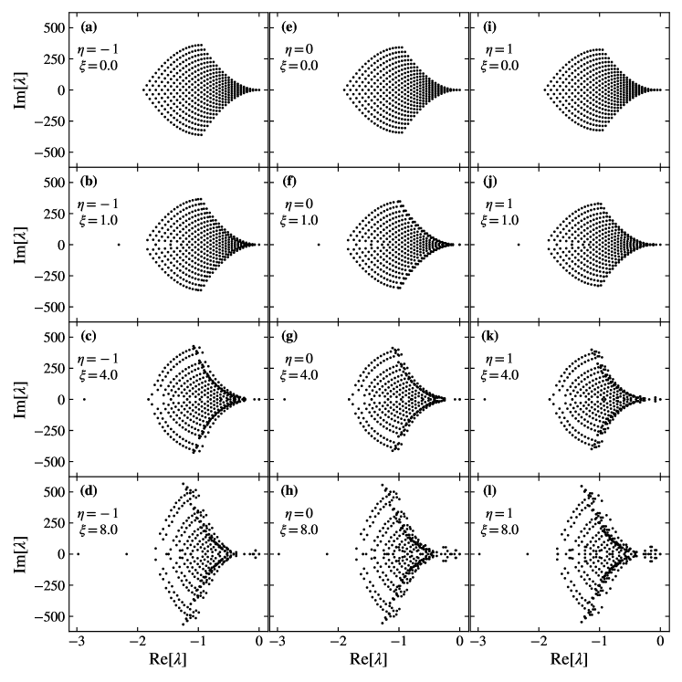
Figure 6: Scatterplot of the squeezed Kerr oscillator for $\eta=\omega/K=-1,0,+1$, $\xi=\varepsilon_{2}/K=0.0,1.0,4.0,8.0$, and $N_{\rm Fock}=20$.

As $\xi$ increases, one can observe the formation of structures similar to those of figure 4. These structures are particularly evident for $\xi=4.0$ and $\xi=8.0$. Their actual form is similar but not identical to that of figure 4, since here the energy of the states belonging to the representation $\left|j^{\prime},m^{\prime}\right\rangle$ of $su(2)$ are $E_{m^{\prime}_{j^{\prime}}}=|m^{\prime}_{j^{\prime}}|$ [21] and not $E_{m^{\prime}_{j^{\prime}}}={m^{\prime}_{j^{\prime}}}^{2}$.

This form is illustrated in figure 7a, where the portion $\left|\mathrm{Re}\left[\lambda\right]\right|\leq 1$ of the scatterplot for $\eta=\omega/K=0$, $\xi=\varepsilon_{2}/K=12.0$ is shown, with doubly degenerate points marked in red. The two phases are clearly separated here. The structure of Phase II is a perturbed form of a doubly degenerate anharmonic oscillator with energies given approximately by equation (52) of [21],

$$E_{\nu}^{\pi}=4\xi\nu\left(1-\frac{\nu}{N_{\rm eff}}\right)$$ (57)

where $\nu^{\pi}$ $(\nu=0,1,...;\pi=\pm)$ denotes the quantum states, and $N_{\rm eff}=N_{\rm conv}/2$ where $N_{\rm conv}$ is the value $N_{\rm Fock}-1$ of states required in the numerical calculation for convergence of eigenvalues in Phase II. The Liouvillian spectrum of the oscillator is

$$\lambda_{\nu,\nu^{\prime}}=-\rmi\left(E_{\nu}-E_{\nu^{\prime}}\right)-\frac{\kappa}{2}\left(\nu+\nu^{\prime}\right)$$ (58)

shown in figure 7b. For the first three branches, the imaginary parts of Phase II eigenvalues, $\mathrm{Im}\left[\lambda\right]$, follow closely (58). However, the real parts, $\mathrm{Re}\left[\lambda\right]$, are highly perturbed. Moreover, the fourth branch consisting of a single doubly degenerate point does not appear in panel (a) due to mixing with the singly degenerate states of Phase I.

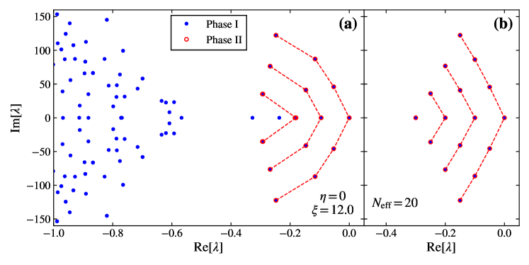
Figure 7: (a) Portion $\left|\mathrm{Re}\left[\lambda\right]\right|\leq 1$ of the scatterplot of the squeezed Kerr oscillator for $\eta=\omega/K=0$ and $\xi=\varepsilon_{2}/K=12.0$. Doubly degenerate points belonging to Phase II are colored in red. Here $N=80=2N_{\rm conv}$ to ensure convergence of Phase I and Phase II eigenvalues for $\xi=12.0$. (b) Scatterplot of the doubly degenerate anharmonic oscillator of (58) with $\nu=0,1,2,3$, $\pi=\pm$, and $N_{\rm eff}=20$. All points are doubly degenerate and colored in red.

In order to clarify further the situation, we consider next the evolution of the eigenvalues of the Liouville superoperator for the squeezed Kerr oscillator as a function of the parameter $\xi=\varepsilon_{2}/K$ separated into real and imaginary part. In figure 8, we show $\mathrm{Re}[\lambda_{i}]$ and $\mathrm{Im}[\lambda_{i}]$ for the first nine eigenvalues. From this figure one can see that $\mathrm{Re}[\lambda_{1}]$ for $\eta=1$ has a discontinuity around $\xi=0$. To clarify this behavior we show in figure 9 a close up of $\mathrm{Re}[\lambda_{i}]$ for small $\xi$. The discontinuity is related to a 1st order QPT which will be discussed in the following section.

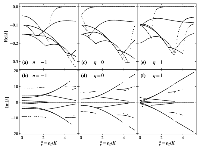
Figure 8: The lowest eigenvalues $\lambda_{i}(i=1,...,9)$ of the Liouville superoperator for the Kerr oscillator for $\eta=\omega/K=-1,0,+1$ as a function of $\xi=\varepsilon_{2}/K$.

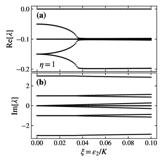
Figure 9: The small $\xi$ behavior of $\mathrm{Re}[\lambda_{i}]$ for the Kerr oscillator for $\eta=+1$.

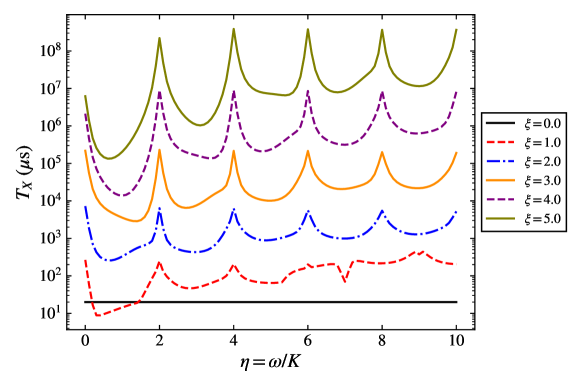
Figure 10: The relaxation time $T_{X}$ of the squeezed Kerr oscillator for $0\leq\eta\leq 10$, $0\leq\xi\leq 5$, and $\kappa=0.1$ $\mu$s^-1.

From the lowest nonzero eigenvalue $\lambda_{1}$ we can calculate the relaxation time

$$T_{X}=-\frac{1}{\mathrm{Re}[\lambda_{1}]}$$ (59)

shown in figure 10 for some values of $\xi$ and as a function of $\eta$. We see that for large $\xi$ a characteristic behavior emerges, that is for even values of the parameter $\eta$ the relaxation time is larger than for odd values. The peak at $\eta=2$ already appears for $\xi=0.5$, while those at $\eta=4,6,8,10$ appear at $\xi=\eta/4=1,1.5,2.0,2.5$. These peaks at integer $\eta$ can be attributed to the quasi-spin symmetry of the Liouvillian maintained at nonzero $\xi$, discussed previously. Maxima in $T_{X}$ occur at even $\eta$ due to degeneracies of Hamiltonian eigenvalues maintained for finite $\xi$ and smaller $T_{X}$ occur at odd $\eta$ due to avoided level crossings. These Hamiltonian properties are further discussed in [21]. This result is of particular importance for quantum computing, since it shows that by appropriately tuning the parameters one can devise systems with large relaxation time.

5 QPT and ESQPT in open systems

5.1 QPT and ESQPT of the Hamiltonian operator

Quantum Phase Transitions (QPT) [22] and associated Excited State Quantum Phase Transitions (ESQPT) [23, 24, 25] of Hamiltonian operators have been extensively studied in a variety of systems [44], especially for algebraic models with structure $g\equiv su(n)$ [23]. For the Hamiltonian operator the consequences of a QPT are: (i) the ground state energy $E_{0}$ is a non-analytic function of the control parameter at $\xi=\xi_{\rm c}$; (ii) the ground state wave function properties, expressed via “order parameters”, i.e. the expectation value of some suitable chosen operator $\left\langle\hat{o}\right\rangle$, are non-analytic at $\xi=\xi_{\rm c}$; (iii) the energy gap $\Delta_{E_{1}}=E_{1}-E_{0}$ between the ground state and the first excited state vanishes at $\xi=\xi_{\rm c}$. For finite systems with $N$ constituents, the defining characteristic of a QPT is not the presence of a true singularity but rather well-defined scaling properties of the relevant quantities towards their singular $N\rightarrow\infty$ limits, called the thermodynamic limit. QPTs are called 0th, 1st, 2nd,… order if the discontinuity occurs in the ground state energy, $E_{0}$, or in the first, second,… derivative $\partial E_{0}/\partial\xi,\partial^{2}E_{0}/\partial\xi^{2},...$ (Ehrenfest classification). In the associated order parameter $\left\langle\hat{o}\right\rangle$, the discontinuities occur for first order in $\left\langle\hat{o}\right\rangle$, second order in $\partial\left\langle\hat{o}\right\rangle/\partial\xi$, …

The Hamiltonian operator $\hat{H}$ of (56) has two control parameters, $\eta$ and $\xi$. It has already been found that, for $\eta=0$ and $\xi=0$, there is a 2nd order QPT and, as a function of $\xi$, an associated ESQPT [26, 27]. The phase structure of the Hamiltonian operator of the squeezed Kerr oscillator is however more complicated than a single 2nd order transition.

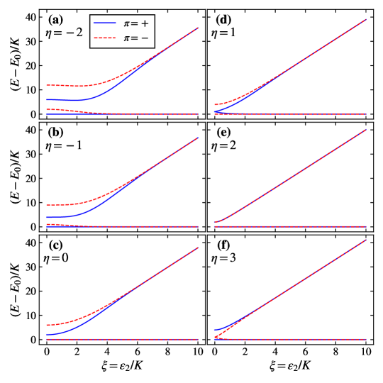
Figure 11: The energy levels of the squeezed Kerr oscillator as a function of $\xi$ for $-2\leq\eta\leq+3$. Levels are labeled by parity $\pi=\pm$.

To illustrate this point, we show in figure 11 a plot of the lowest four energy levels as a function of $\xi$ for $-2\leq\eta\leq+3$. One can see here clearly the occurrence of property (iii) (vanishing of the Hamiltonian gap), indicating a transition at values $\xi_{\rm k}$ given by $\xi_{\rm k}=-2\eta$ for $\eta=-2,-1,0$, but a more complex structure for $\eta>0$. The value $\xi_{\rm k}$ at which $\Delta_{E_{1}}=E_{1}-E_{0}=0$ is also called a “kissing point”, hence the index $\rm k$ given to $\xi$.

In figure 12, we show a plot of the lowest four energy levels as a function of $\eta$ for $0\leq\xi\leq 5$. The behavior of the energy levels as a function of $\eta$ for fixed $\xi$ is rather complex. At $\xi=0$, it is dictated by the quasi-spin symmetry $su(2)$, as shown in A. It consists in a succession of crossing of levels of opposite parity at integer values of $\eta=0,1,2,$… At $\xi>0$ the level crossings persist, as seen for example at $\xi=1$ and $\xi=2$, but for large $\eta$ and/or large $\xi$ levels become doubly degenerate. This situation, with the occurrence of three phases I, II, III was described in detail in [21]. Its description in terms of phase transitions is rather complex and it requires the study of the classical limit of the algebraic Hamiltonian. We therefore defer it to a later publication.

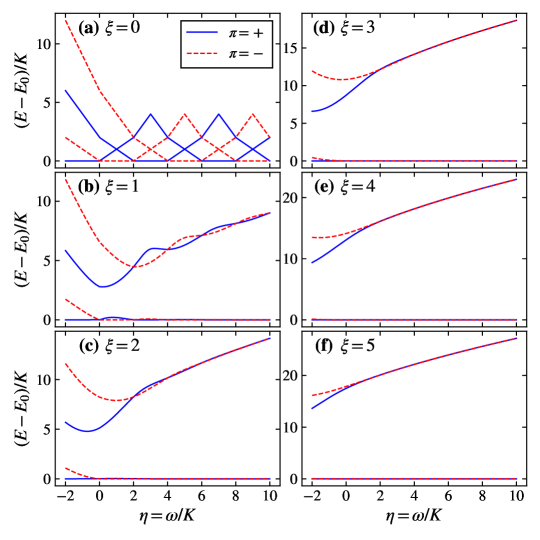
Figure 12: The energy levels of the squeezed Kerr oscillator as a function of $\eta$ for $\xi=0,1,...,5$. Levels are labeled by parity $\pi=\pm$.

For 2nd order transitions of Hamiltonian operators, it is possible to find scaling properties and study the so-called thermodynamic limit $N\rightarrow\infty$, as, for example, in [45]. To this end, it is convenient to construct the scaled Hamiltonian

$$\frac{\hat{H}}{K}=-\eta\hat{n}+\frac{1}{N}\hat{n}(\hat{n}-1)-\chi\hat{P}_{2}$$ (60)

where $N=N_{\rm Fock}-1$ and $\chi=\xi/N$. At the critical point of a phase transition, all properties are expected to scale as a power law $N^{-A}$, where $A$ is the scaling exponent. Particularly important is the order parameter, $\nu=\left\langle\hat{n}_{0}(\chi)\right\rangle/N$, which scales as $\nu(\chi_{\rm c})=A_{n0}N^{-A_{n1}}$. The order parameter as a function of $\chi$ is shown in figure 13 for $\eta=-1$ and different values of $N$. For the Hamiltonian operator with truncated Hilbert space $\mathcal{H}$ of dimension $N_{\rm Fock}=N+1$, it is possible to carry out calculations with large values of $N$ and thus identify the critical point and scaling behavior accurately. The phase transition is 2nd order since, at the critical point $\chi_{\rm c}=0.5$, the first derivative of the order parameter $\nu$ is discontinuous (Ehrenfest classification).

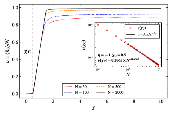
Figure 13: Order parameter for $\eta=-1$ as a function of $\chi$ for different values of $N$. The critical value is $\chi_{\rm c}=0.5$, shown by a dashed vertical line. The scaling behavior of the order parameter at $\chi_{\rm c}$ is plotted in the insert.

The scaling behavior of the order parameter for the $\eta=-1$ case is $\nu(\chi_{\rm c})=0.2065\times N^{-0.6365}$. A similar situation occurs for $\eta=-2$ and $\eta=0$. The critical value is $\chi_{\rm c}=-\frac{1}{2}\eta$. Note that the critical point $\chi_{\rm c}$ is not equal to the kissing point $\xi_{\rm k}$, rather, they are related by $\chi_{\rm c}=\frac{1}{4}\xi_{\rm k}$.

5.2 QPT and ESQPT of the Liouville superoperator

The Liouville superoperator of (4) contains three control parameters, $\eta=\omega/K,\xi=\varepsilon_{2}/K$ and $\zeta=\kappa/K$, the latter being the ratio of the dissipator, $\kappa$, to the Kerr coefficient, $K$. Minganti et al. [33] provided a formal definition of a QPT of order $M$ for open system,s similar to the Ehrenfest classification of QPTs of Hamiltonian operators mentioned in section 5.1,

$$\lim_{\xi\rightarrow\xi_{\rm c}}\left|\frac{\partial^{M}}{\partial\xi^{M}}\lim_{N\rightarrow\infty}Tr\left[\hat{\rho}_{ss}(\xi,N)\hat{o}\right]\right|=+\infty.$$ (61)

In this definition, the ground state of $\hat{H}$, $E_{0}$, is replaced by the steady-state density matrix $\hat{\rho}_{ss}$, which is a normalized eigenmatrix of the Liouvillian corresponding to a zero eigenvalue, $\lambda_{0}=0$, $\hat{\rho}_{ss}=\hat{\rho}_{0}/\mathrm{Tr}\left[\hat{\rho}_{0}\right]$. While in the case of closed systems one needs to consider the eigenvalues of $\hat{H}$ as in figures 11 and 12, for open systems one must consider the eigenvalues $\lambda_{i}$ of the Liouville superoperator $\mathcal{L}$, ordered in such a way that $\left|\mathrm{Re}\left[\lambda_{0}\right]\right|<\left|\mathrm{Re}[\lambda_{1}]\right|<...<\left|\mathrm{Re}[\lambda_{n}]\right|$, and then look at their properties.

5.2.1 Second order QPT of the squeezed Kerr oscillator.

The study of 2nd order QPT of the Liouville superoperator is straightforward, as one needs to consider only the first non-zero eigenvalue $\lambda_{1}$. The real part $\mathrm{Re}[\lambda_{1}]$ (Liouvillian gap), called also the asymptotic decay rate [34], is of importance since it determines the slowest relaxation time of the system in the long-time limit, $T_{X}$ (59).The imaginary part $\mathrm{Im}[\lambda_{1}]$, called the Hamiltonian gap, is also relevant, since at the critical point it closes [34], [46] and the levels touch.

To illustrate these properties, we consider now two cases, $\eta=-1$ and $\eta=0$. Consider first the case of $\eta=-1$, called the squeezed quadratic oscillator, with Hamiltonian

$$\frac{\hat{H}}{K}=\hat{n}^{2}-\xi\hat{P}_{2}$$ (62)

and Liouville superoperator as in (4). A similar case was also considered in [33], but with quadratic dissipation also included. The real and imaginary parts of the eigenvalue $\lambda_{1}$ as a function of $\xi$ for $N=100$ are shown in figure 14a,b. One can see clearly the occurrence of a phase transition. In $\mathrm{Im}[\lambda_{1}]$ the second order QPT appears as the closing of the Hamiltonian gap at $\xi_{\rm k}=2$. In $\mathrm{Re}[\lambda_{1}]$ it appears as a minimum. The relaxation time $T_{X}$ is shown in figure 14c. Here the QPT appears as a minimum at $\xi_{\rm k}=2$.

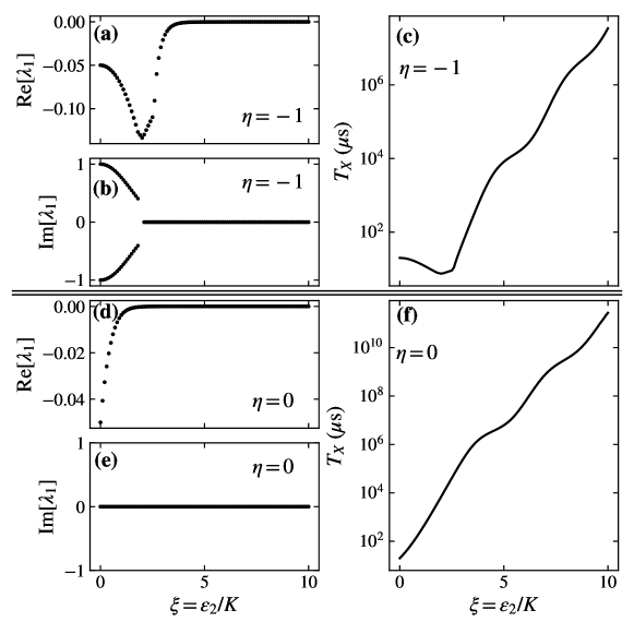
Figure 14: Top: (a) $\mathrm{Re}[\lambda_{1}]$ and (b) $\mathrm{Im}[\lambda_{1}]$ as a function of $\xi$ for the squeezed quadratic oscillator. (c) The relaxation time $T_{X}$ as a function of $\xi$ for the squeezed quadratic oscillator. Bottom: (d) $\mathrm{Re}[\lambda_{1}]$ and (e) $\mathrm{Im}[\lambda_{1}]$ as a function of $\xi$ for the squeezed Kerr oscillator. (f) The relaxation time $T_{X}$ as a function of $\xi$ for the squeezed Kerr oscillator.

Consider next the case $\eta=0$, called the squeezed Kerr oscillator, with Hamiltonian

$$\frac{\hat{H}}{K}=\hat{n}(\hat{n}-1)-\xi\hat{P}_{2}.$$ (63)

The real and imaginary parts of the eigenvalue $\lambda_{1}$ as a function of $\xi$ for $N=100$ are shown in figure 14d,e. The QPT here is not seen because it is obscured by the fact that the kissing point is at $\xi_{\rm k}=0$. The relaxation time is shown in figure 14f.

We now consider the scaling properties of the squeezed quadratic oscillator, $\eta=-1$, with scaled Hamiltonian as in (60) and linear dissipator of (4). Scaling properties now depend also on $\zeta=\kappa/K$ and one needs to consider both the order parameter $\nu=\left\langle\hat{n}_{0}\right\rangle/N$ and the Liouvillian gap, $\Delta=-\mathrm{Re}[\lambda_{1}]$. While the former is a property of the Hamiltonian and appears in section 5.1, the latter appears only for dissipative phase transitions. These quantities are shown in figure 15, as a function of $\chi$ for a fixed value of $\zeta=0.1$. A similar calculation of the order parameter was done previously in [33].

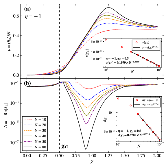
Figure 15: (a) The order parameter $\nu=\left\langle\hat{n}_{0}\right\rangle/N$ as a function of $\chi$ for $\zeta=0.1$; (b) The Liouvillian gap $\Delta=-\mathrm{Re}[\lambda_{1}]$ as function of $\chi$ for $\zeta=0.1$. Both in (a) and (b) $10\leq N\leq 80$. The critical value $\chi_{\rm c}$ is shown by a dashed vertical line. The scaling behavior of $\nu(\chi_{\rm c})$ is plotted in the insert in (a), and the scaling behavior of $\Delta\chi_{1}=\chi_{\max}-\chi_{\rm c}$ is plotted in the insert in (b).

We first note that the Hilbert space $\mathcal{H}\otimes\mathcal{H}$ of the Liouvillian is of dimension $N_{\rm Fock}\times N_{\rm Fock}$, and therefore we consider values $N\leq 80$ for computational purposes, in contrast with studies of the Hamiltonian. We also note that in figure 15a the critical value of the order parameter $\nu$ is the same as for the Hamiltonian for $\eta=-1$, $\chi_{\rm c}=0.5$, and that the transition is of 2nd order since the slope of $\nu$ is discontinuous at $\chi_{\rm c}$ in the $N\rightarrow\infty$ limit. This property was also emphasized in a recent preprint where experimental results were presented [47]. The scaling exponent, shown in the insert of figure 15a is however different from that of the Hamiltonian, $\nu(\chi_{\rm c})=0.1979\times N^{-0.4699}$, indicating a dependence on $\zeta$ (here $\zeta=0.1$). As the discontinuity here is smoothed out by finite $N$ effects, in figure 16 we display a close up view of $\nu$, $\Delta$, and $\frac{\rm{d}\nu}{\rm{d}\chi}$ around the critical point to better illustrate behavior at $\chi_{\rm c}$ and the discontinuity in $\frac{\rm{d}\nu}{\rm{d}\chi}$. Another feature apparent in figure 15a is the maximum occurring at about $\chi\cong 1.25$ before $\nu$ approaches its asymptotic value of $\nu=1/2$. This maximum is also related to finite $N$ effects and is a result of approximating a piecewise discontinuous function by a continuous one, sometimes called the Gibbs phenomenon [48].

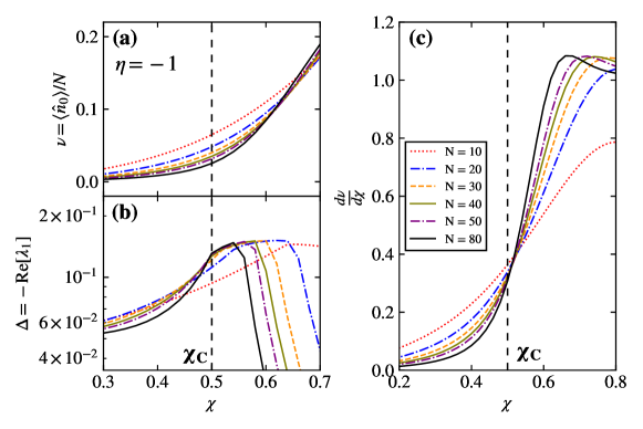
Figure 16: An enlarged version of the region around the critical point $\chi_{c}$ of figure 15. (a) Order parameter; (b) Liouvillian gap; (c) First derivative of the order parameter, $\frac{\rm{d}\nu}{\rm{d}\chi}$, plotted to emphasize its discontinuous behavior near $\chi_{c}$.

Of particular interest is the behavior of the Liouvillian gap $\Delta=-\mathrm{Re}\left[\lambda_{1}\right]$ in figure 15b. At the critical point $\chi_{c}=0.5$, $\Delta$ approaches a maximum value in the $N\rightarrow\infty$ limit, as expected from the previous figure 14a for the unscaled system, where $\mathrm{Re}\left[\lambda_{1}\right]$ has a minimum. This behavior is apparent in figure 16b. Several quantities can be used to describe the scaling behavior of $\Delta$. We use here the quantity $\Delta\chi_{1}=\chi_{\max}-\chi_{c}$, where $\chi_{\max}$ is the value of $\chi$ at the maximum value attained by $\Delta$, e.g. $\Delta\left(\chi_{\max}\right)=\max\left[\Delta\right]$. The scaling behavior of this quantity is shown in the insert of figure 15b, as $\Delta\chi_{1}=0.6706\times N^{-0.5716}$.

Another important feature of figure 15b is the minimum of $\Delta$ occurring at $\chi_{\min}\cong 0.9$. This minimum, found at large values of $\chi=\xi/N$, was not noted in [33], since the calculation was stopped at values less than $\chi_{\min}$. The minimum occurs at ultrastrong values of the squeezing strength $\xi_{\min}\cong 0.9N$, which diverge as $N\rightarrow\infty$. The study of this ultrastrong regime is outside the scope of the present article.

5.2.2 First order QPT of the squeezed Kerr oscillator.

The study of first order QPTs, both non-dissipative and dissipative, is more complicated than that of second order. For the Hamiltonian operator, first order QPTs were investigated in complex algebraic models [44] either, years ago, in models in large numbers of dimensions such as the $su(6)$ interacting boson model [49], or, more recently, in coupled Bose-Fermi systems such as the Dicke or Rabi Models [50, 51].

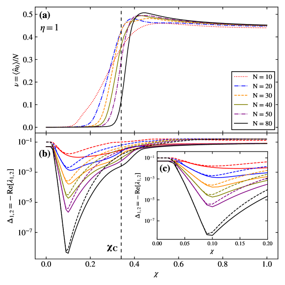
Figure 17: (a) The order parameter $\nu$ as a function of $\chi$ for $\zeta=0.1$; (b) The Liouvillian gaps $\mathrm{Re}[\lambda_{1}]$ (full line), $\mathrm{Re}[\lambda_{2}]$(dashed line), as a function of $\chi$ for $\zeta=0.1$; (c) close-up of the Liouvillian gap for small $\xi\leq 0.2$. The dashed vertical line indicates the value of $\chi_{\rm c}$ at $N=80$.

In the case of higher-dimensional models [3] it was found [49] that one needs more than one excited eigenvalue, $E_{1}$, to study 1st order transitions. The complications found in the study of 1st order QPTs of Hamiltonian operators are even more apparent in the study of 1st order QPTs of Liouville superoperators. In [33], it was suggested to consider two non-zero eigenvalues $\lambda_{1}$ and $\lambda_{2}$ of the Liouville superoperator. Here, we consider specifically the case of $\eta=+1$, with scaled Hamiltonian of (60) and linear dissipator of (4), and study its order parameter $\nu$ and the real parts of its eigenvalues $\mathrm{Re}[\lambda_{1}]$, $\mathrm{Re}[\lambda_{2}]$. These quantities are shown in figure 17 as a function of $\chi$ for $\zeta=0.1$.

In figure 17a one can clearly see the discontinuity in the order parameter $\nu$ (a property of the lowest eigenstate) indicating a first order QPT (Ehrenfest classification). As $N$ increases, the value $\chi_{\rm c}$ at which the discontinuity occurs increases. At $N=80$ it is $\chi_{\rm c}\cong 0.34$. We estimate by extrapolation that in the asymptotic limit, $N\rightarrow\infty$, $\chi_{\rm c}=0.4$. The behavior of the Liouvillian gap is more complicated. Both $\Delta_{1}=-\mathrm{Re}[\lambda_{1}]$ and $\Delta_{2}=-\mathrm{Re}[\lambda_{2}]$ have a minimum. Up to $\chi\cong 0.10$, the values of $\Delta_{1}$ and $\Delta_{2}$ are degenerate. From that point on, they split. The first order QPT which occurs for the order parameter $\nu$ at $\chi_{\rm c}\cong 0.34$ (for $N=80$), appears in the Liouvillian gap as an inflection point in $\Delta_{1}$, observed in figure 17b. The properties of the Liouvillian gap for small values of $\chi$ observed in figure 17b-c are consistent with panel (e) of figure 8. We also note that the behavior of the Liouvillian gap as a function of $\chi$, while similar to that of [33] for small $\chi\leq 0.1$, differs for $\chi\geq 0.1$. The difference may be due to the fact that the authors in [33] included also a quadratic dissipator, and that we take the asymptotic thermodynamic limit to be $N\rightarrow\infty$ where $N$ is the maximum number of bosons, $N=N_{\rm Fock}-1$.

6 Temperature dependence

In this section we consider the temperature dependence of the eigenvalues of the Liouville superoperator $\mathcal{L}$ and the relaxation time $T_{X}$.

6.1 Harmonic oscillator

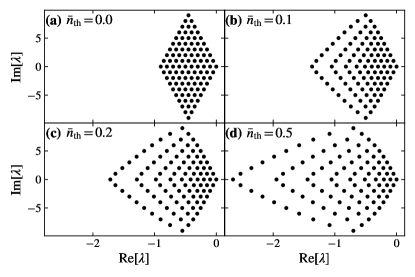
Figure 18: Temperature dependence of the eigenvalue spectrum of the harmonic oscillator with $N_{\rm Fock}=10$ for $\bar{n}_{\rm th}=0.0,0.1,0.2,0.5$.

For the truncated harmonic oscillator, $\omega=-1,$ $K=0$, the spectrum of eigenvalues of the Liouville superoperator is shown in figure 18 for $N_{\rm Fock}=10$ and average temperatures $\bar{n}_{\rm th}=0,0.1,0.2,0.5$. The effect of the temperature is to deform the spectrum from the rhombic structure of panel (a) to the dilated structure of panels (b-d). The real part of the eigenvalue $\lambda_{1}$ changes from $\mathrm{Re}[\lambda_{1}]=-0.050$ at $\bar{n}_{\rm th}=0$ to $\mathrm{Re}[\lambda_{1}]=-0.078$ at $\bar{n}_{\rm th}=0.1$. Correspondently, the relaxation time for $\kappa=0.1$ $\mu$s^-1 changes from $T_{X}=20$ $\mu$s to $T_{X}=12.8$ $\mu$s. It is important to note that truncation and finite $N$ effects are important for finite temperature, especially as $\bar{n}_{\rm th}$ increases.

6.2 Kerr oscillator

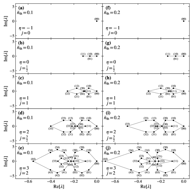
Figure 19: Temperature dependence of the eigenvalue spectrum of the Liouvillian of the Kerr oscillator with $N_{\rm Fock}=10$. Points are labelled by the (here approximate) values of $(n,m)$ for comparison with figure 4.

For the Kerr oscillator, $\omega=-1,0,1,2,3,$ $K=1,$ $\varepsilon_{2}=0$, we show in figure 19, the deformation of the eigenvalues of the Liouvillian for the quasi-spin representation $\left|j,m_{j}\right\rangle$ of figure 4 when going from $\bar{n}_{\rm th}=0$ to $\bar{n}_{\rm th}=0.2$. It appears that the geometric double ellipsoidal structure of the eigenvalues persists, although somewhat deformed. Also, the degeneracy of the middle point is lifted.

6.3 Squeezed Kerr oscillator

Here we present results for the squeezed Kerr oscillator, $\eta=\omega/K=-1,0,$ $\xi=\varepsilon_{2}/K\neq 0$. The behavior of the relaxation time $T_{X}$ as a function of $\bar{n}_{\rm th}$ for several values of $\xi$ and $\eta$ was investigated in great detail in [19]. Here we show in figure 20a-b the behavior of $\mathrm{Re}[\lambda_{1}]$ as a function of $\xi$ for several values of $\bar{n}_{\rm th}$ between $0.0$ and $1.0$ and $\eta=-1,0$. One can clearly see the second order dissipative QPT occurring at $\xi_{\rm k}\cong 2.0$ for $\eta=-1$ and a smoother behavior for $\eta=0$ where the QPT occurs at $\xi=0$ and it is thus masked when $\xi>0$. From $\mathrm{Re}[\lambda_{1}]$, we can calculate the relaxation time $T_{X}=-\frac{1}{\mathrm{Re}[\lambda_{1}]}$ as a function of $\xi$, given in figure 20c-d. Here, we see a dramatic decrease of the relaxation time even for small $\bar{n}_{\rm th}=0.1$. This behavior is emphasized in the subsequent figure 21, which shows the relaxation as a function of $0.0\leq\bar{n}_{\rm th}\leq 1.0$ for $\eta=-1$ and $\eta=0$. A similar situation occurs for the relaxation time as a function of $\eta$ [19], shown in figure 22 for $\xi_{\rm k}=2.0$ and several values of $\bar{n}_{\rm th}$ between $0.0$ and $1.0$. One can see here that although the peaked structure for $\eta=\mathrm{even}$ persists even at large temperatures, it is gradually washed away. These results stress that while the squeezed Kerr oscillator can be parametrically tuned to maximize relaxation time, thermal effects and maintaining low temperatures are equally important to doing so.

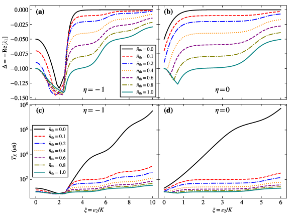
Figure 20: Behavior of $\mathrm{Re}[\lambda_{1}]$ as a function of $\xi$ for several values of $\bar{n}_{\rm th}$ and $\eta=-1$ (a)$,\eta=0$ (b). Behavior of $T_{X}$ as a function of $\xi$ for several values of $\bar{n}_{\rm th}$ and $\eta=-1$ (c), $\eta=0$ (d).

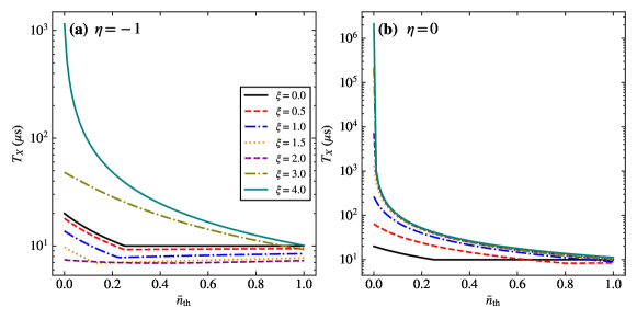
Figure 21: Behavior of $T_{X}$ as a function of $0\leq\bar{n}_{\rm th}\leq 1.0$ for several values of $\xi$ and $\eta=-1$ (a)$,\eta=0$ (b).

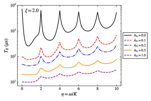
Figure 22: Behavior of $T_{X}$ as a function of $\eta=\omega/K$ for $\xi=2$ and several values of $\bar{n}_{\rm th}$. In this figure, $\kappa=0.1$ $\mu$s^-1.

7 Summary and conclusions

In this article, we have investigated the symmetries of the Liouville superoperator, $\mathcal{L}$, of one-dimensional parametric oscillators, especially the squeeze-driven Kerr oscillator. We have shown that for integer values of the ratio $\eta=\omega/K$ in the Kerr Hamiltonian $\hat{H}=-\omega\hat{n}+K\hat{n}(\hat{n}-1)$, the spectrum of $\mathcal{L}$ has a characteristic double-ellipsoidal structure and an hitherto unknown $su(2)$ quasi-spin symmetry, which reflects the symmetry of the Hamiltonian $\hat{H}$. We have also shown that, as a result of this quasi-spin symmetry, the relaxation time $T_{X}$ is particularly large for even integer values of the ratio $\eta$ in the squeeze-driven Hamiltonian $\hat{H}=-\omega\hat{n}+K\hat{n}(\hat{n}-1)-\varepsilon_{2}\hat{P}_{2}$, a result of importance for the generation of long-lived states useful in quantum computing. On the other hand, we have shown that at nonzero temperature the relaxation time $T_{X}$ decreases dramatically, even for low thermal populations $\bar{n}_{\rm th}\cong 0.1$. Our combined results suggest that ‘optimal’ Kerr devices are for $\eta=\mathrm{even}=4,6,...,\xi=\rm{large}\geq 4.0$, kept at the lowest possible temperature, $\bar{n}_{\rm th}\leq 0.1$.

The results presented here can be extended to oscillators with higher order squeezing, cubic, $k_{\rm s}=3$, and quartic, $k_{\rm s}=4$, which can be realized experimentally [18, 19] and to higher order dissipation, such as quadratic, $k_{\rm d}=2$, and cubic, $k_{\rm d}=3$, which may play a role in experiments [19]. Our results are also of relevance to all parametric one-dimensional oscillators and to all other models with Hamiltonian operators which can be cast in the form of non-linear squeezed oscillators. This includes the Lipkin model, with Hamiltonian

$$\hat{H}=\omega\hat{J}_{z}+K\hat{J}_{z}^{2}-\varepsilon_{2}(\hat{J}_{+}^{2}+\hat{J}_{-}^{2}),$$ (64)

and dissipators $\mathcal{D}[\hat{J}_{\pm}]\hat{\rho}(t)$ [43] which, together with the Kerr oscillator and the one-dimensional vibron model, form a “universality class” of parametric oscillators.

Our recognition that the Liouville superoperator of the Kerr oscillator has a quasi-spin symmetry $su(2)$ reflecting the symmetry of its Hamiltonian has major implications for the study of Open Parametric Oscillators (OPO) [9, 10]. The study of symmetries of the Liouvillian performed here can be extended to two coupled oscillators, $su_{1}(2)\oplus su_{2}(2)$, in the same way in which is done in nuclear physics for the proton-neutron interacting boson model, $su_{1}(6)\oplus su_{2}(6)$ [3], and in molecular physics for triatomic molecules, $su_{1}(4)\oplus su_{2}(4)$ [4], and most importantly, to a large number of coupled oscillators on a lattice $\sum_{i}\oplus su_{i}(2)$, in the same way in which it is done in the algebraic theory of crystal vibrations [52, 53].

Finally, the study of symmetries and dissipative quantum phase transitions of Liouvillian presented here can be extended to more complex models, such as the Rabi, Dicke and Jaynes-Cummings models [50, 51], the Hamiltonian of which is expressed in terms of boson, $\hat{a}^{{\dagger}},\hat{a}$ and fermion, $\hat{\sigma}_{x},\hat{\sigma}_{y},\hat{\sigma}_{z}$, operators and for which the quantum phase transitions of the Hamiltonian have already been studied [50, 51].

Appendix A Review of the quasi-spin symmetry $\mathbf{su(2)}$

Consider the dimensionless Hamiltonian

$$\hat{H}_{1}=\frac{\hat{H}}{K}=-\left(\eta+1\right)\hat{n}+\hat{n}^{2}=-\eta^{\prime}\hat{n}+\hat{n}^{2}$$ (65)

The eigenvalues of $\hat{H}_{1}$ counted from the lowest state are shown in figure 23.

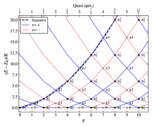
Figure 23: Excitation energy of the Hamiltonian $\hat{H}_{1}$ (65) as a function of the parameter $\eta=\omega/K$ showing the degeneracies that occur for integer values of the parameter $\eta$ and the classification of states in terms of quasi-spin quantum numbers $\left|j,m_{j}\right\rangle$. States are colored by parity, and the separatrix, marked with a black dashed line, $E_{s}/K=\eta/2+\eta^{2}/4$, divides the spectrum into two phases.

To the left of the dashed line, called the separatrix, states are singly degenerate with eigenvalues $E=-\eta^{\prime}n+n^{2}$. To the right of the separatrix and for $\eta^{\prime}=\eta+1=\mathrm{integer}$, degeneracies occur. The degenerate points can be characterized by quasi-spin quantum numbers $\left|j,m_{j}\right\rangle$. The values of the quasi-spin are $j=\frac{\eta^{\prime}}{2}=\frac{\eta+1}{2}$, while those of $m_{j}$ are

$$m_{j} = \pm j,\pm\left(j-1\right),...,\pm 1/2;\quad j=\mathrm{half-integer};\quad\eta=\mathrm{even}$$

$$m_{j} = \pm j,\pm\left(j-1\right),...,0;\quad j=\mathrm{integer};\quad\eta=\mathrm{odd}.$$ (66)

The eigenvalues $E_{m}$ are given by

$$E_{m}=m_{j}^{2}-j^{2}.$$ (67)

When counted from the lowest state, they can be written as

$$E_{m} = m_{j}^{2}-1/4\quad j=\mathrm{half-integer}$$

$$E_{m} = m_{j}^{2}\qquad j=\mathrm{integer}.$$ (68)

Both sets of eigenvalues correspond to the quasi-spin symmetry $su(2)\supset so(2)$. To further elucidate this quasi-spin symmetry, it is convenient to explicitly construct the representations $\left|j,m_{j}\right\rangle$ with two boson operators $\hat{b}_{1},\hat{b}_{2}$ with eigenvalues of the number operators $\hat{n}_{1},\hat{n}_{2}$ satisfying $n_{1}+n_{2}=N$. In this situation, products of the two boson operators, $\hat{b}_{1}^{{\dagger}}\hat{b}_{2}$, $\hat{b}_{2}^{{\dagger}}\hat{b}_{2}$, $\hat{n}_{1}=\hat{b}_{1}^{{\dagger}}\hat{b}_{1}$, $\hat{n}_{2}=\hat{b}_{2}^{{\dagger}}\hat{b}_{2}$, form the Lie algebra $u(2)$, and the degenerate states of the Hamiltonian $\hat{H}_{1}$ can be realized by letting $\hat{n}=\hat{n}_{1}$ in (65) and $N=\eta^{\prime}=2j$. The minimum energy is found to be $E_{\rm min}=-\eta^{\prime 2}/4+1/4$ for $\eta^{\prime}=\mathrm{odd}$ and $E_{\rm min}=-\eta^{\prime 2}/4$ for $\eta^{\prime}=\mathrm{even}$, yielding energies counted from the lowest state,

$$E_{n}-E_{\rm min} = n_{1}^{2}-\eta^{\prime}n_{1}+\eta^{\prime 2}/4-1/4\quad\eta^{\prime}=\mathrm{odd}$$

$$E_{n}-E_{\rm min} = n_{1}^{2}-\eta^{\prime}n_{1}+\eta^{\prime 2}/4\qquad\eta^{\prime}=\mathrm{even}.$$ (69)

These formulae can be converted to the $su(2)$ quasi-spin notation, $\left|j,m_{j}\right\rangle$, by noting $n_{1}+n_{2}=N=\eta^{\prime}=2j$, and using,

$$j=\left(\frac{n_{2}+n_{1}}{2}\right),\quad m_{j}=\left(\frac{n_{2}-n_{1}}{2}\right)$$ (70)

to explicitly obtain (A) from (A). Furthermore, we can compactly write the Hamiltonian $\hat{H}_{1}$, counting from the lowest energy state, in the $N=2j$ subspace of the full Hilbert space in terms of quasi-spin operators,

$$\hat{H}_{1}=\hat{j}_{z}^{2}-\frac{1}{8}\left(1-(-1)^{2j}\right)$$ (71)

where $\hat{j}_{z}\left|j,m_{j}\right\rangle=m_{j}\left|j,m_{j}\right\rangle$. The quasi-spin dynamic symmetry of $\hat{H}_{1}$ is evident here as it is written exclusively in terms of the $su(2)\supset so(2)$ invariant Casimir operator $\hat{j}_{z}$.

In terms of the two boson operators $\hat{b}_{1},\hat{b}_{2}$, the wave functions of the degenerate states can be written as

$$\left|n_{1},n_{2}\right\rangle=\frac{1}{\sqrt{n_{1}!\left(N-n_{1}\right)!}}\left(\hat{b}_{2}^{{\dagger}}\right)^{N-n_{1}}\left(\hat{b}_{1}\right)^{n_{1}}\left|0\right\rangle$$ (72)

The notation $\left|n_{1},n_{2}\right\rangle$ can be converted to the usual quasi-spin notation by means of (70), giving

$$\left|j,m_{j}\right\rangle=\frac{1}{\sqrt{\left(j-m_{j}\right)!\left(j+m_{j}\right)!}}\left(\hat{b}_{2}^{{\dagger}}\right)^{j+m_{j}}\left(\hat{b}_{1}^{{\dagger}}\right)^{j-m_{j}}\left|0\right\rangle.$$ (73)

Additional details can be found in [21] and [31].

References

References

- [1] Gell-Mann M 1962 Phys. Rev. 125(3) 1067–1084 URL https://link.aps.org/doi/10.1103/PhysRev.125.1067
- [2] Ne’eman Y 1961 Nucl. Phys. 26 222–229 ISSN 0029-5582 URL https://www.sciencedirect.com/science/article/pii/0029558261901341
- [3] Iachello F and Arima A 1987 The Interacting Boson Model Cambridge Monographs on Mathematical Physics (Cambridge University Press)
- [4] Iachello F and Levine R D 1995 Algebraic Theory of Molecules (Oxford University Press) ISBN 9780195080919 URL https://doi.org/10.1093/oso/9780195080919.001.0001
- [5] Lipkin H, Meshkov N and Glick A 1965 Nucl. Phys. 62 188–198 ISSN 0029-5582 URL https://www.sciencedirect.com/science/article/pii/002955826590862X
- [6] Rabi I I 1936 Phys. Rev. 49(4) 324–328 URL https://link.aps.org/doi/10.1103/PhysRev.49.324
- [7] Dicke R H 1954 Phys. Rev. 93(1) 99–110 URL https://link.aps.org/doi/10.1103/PhysRev.93.99
- [8] Jaynes E T and Cummings F W 1963 IEEE Proc. 51 89–109
- [9] Goto H 2016 Sci. Rep. 6 21686 URL https://doi.org/10.1038/srep21686
- [10] Goto H 2019 J. Phys. Soc. Japan 88 061015 URL https://doi.org/10.7566/JPSJ.88.061015
- [11] Mirrahimi M, Leghtas Z, Albert V V, Touzard S, Schoelkopf R J, Jiang L and Devoret M H 2014 New J. Phys. 16 045014 URL https://dx.doi.org/10.1088/1367-2630/16/4/045014
- [12] Puri S, Boutin S and Blais A 2017 npj Quantum Inf. 3 18 URL https://doi.org/10.1038/s41534-017-0019-1
- [13] Grimm A, Frattini N E, Puri S, Mundhada S O, Touzard S, Mirrahimi M, Girvin S M, Shankar S and Devoret M H 2020 Nature 584 205–209 URL https://doi.org/10.1038/s41586-020-2587-z
- [14] Blais A, Grimsmo A L, Girvin S M and Wallraff A 2021 Rev. Mod. Phys. 93(2) 025005 URL https://link.aps.org/doi/10.1103/RevModPhys.93.025005
- [15] Darmawan A S, Brown B J, Grimsmo A L, Tuckett D K and Puri S 2021 PRX Quantum 2(3) 030345 URL https://link.aps.org/doi/10.1103/PRXQuantum.2.030345
- [16] Kwon S, Watabe S and Tsai J S 2022 npj Quantum Inf. 8 40 URL https://doi.org/10.1038/s41534-022-00553-z
- [17] Frattini N E, Cortiñas R G, Venkatraman J, Xiao X, Su Q, Lei C U, Chapman B J, Joshi V R, Girvin S M, Schoelkopf R J, Puri S and Devoret M H 2022 The squeezed kerr oscillator: spectral kissing and phase-flip robustness (Preprint 2209.03934)
- [18] Venkatraman J, Cortinas R G, Frattini N E, Xiao X and Devoret M H 2023 A driven quantum superconducting circuit with multiple tunable degeneracies (Preprint 2211.04605)
- [19] Venkatraman J 2023 Controlling the Effective Hamiltonian of a Driven Quantum Superconducting Circuit Ph.D. thesis Yale University URL https://www.proquest.com/dissertations-theses/controlling-effective-hamiltonian-driven-quantum/docview/2835334119/se-2
- [20] Kirchmair G, Vlastakis B, Leghtas Z, Nigg S E, Paik H, Ginossar E, Mirrahimi M, Frunzio L, Girvin S M and Schoelkopf R J 2013 Nature 495 205–209 URL https://doi.org/10.1038/nature11902
- [21] Iachello F, Cortiñas R G, Pérez-Bernal F and Santos L F 2023 J. Phys. A: Math. Theor. 56 495305 URL https://dx.doi.org/10.1088/1751-8121/ad09eb
- [22] Sachdev S 1999 Quantum Phase Transitions (Cambridge University Press)
- [23] Caprio M, Cejnar P and Iachello F 2008 Ann. Phys., NY 323 1106–1135 ISSN 0003-4916 URL https://www.sciencedirect.com/science/article/pii/S0003491607001042
- [24] Cejnar P and Stránský P 2008 Phys. Rev. E 78(3) 031130 URL https://link.aps.org/doi/10.1103/PhysRevE.78.031130
- [25] Cejnar P, Stránský P, Macek M and Kloc M 2021 J. Phys. A: Math. Theor. 54 133001 URL https://dx.doi.org/10.1088/1751-8121/abdfe8
- [26] Prado Reynoso M A, Nader D J, Chávez-Carlos J, Ordaz-Mendoza B E, Cortiñas R G, Batista V S, Lerma-Hernández S, Pérez-Bernal F and Santos L F 2023 Phys. Rev. A 108(3) 033709 URL https://link.aps.org/doi/10.1103/PhysRevA.108.033709
- [27] Chávez-Carlos J, Lezama T L M, Cortiñas R G, Venkatraman J, Devoret M H, Batista V S, Pérez-Bernal F and Santos L F 2023 npj Quantum Inf. 9 76 URL https://doi.org/10.1038/s41534-023-00745-1
- [28] Lindblad G 1976 Commun. Math. Phys. 48 119–130 URL https://doi.org/10.1007/BF01608499
- [29] Gorini V, Kossakowski A and Sudarshan E C G 1976 J. Math. Phys. 17 821–825 ISSN 0022-2488 (Preprint https://pubs.aip.org/aip/jmp/article-pdf/17/5/821/19090720/821_1_online.pdf) URL https://doi.org/10.1063/1.522979
- [30] Iachello F 1994 Algebraic theory Lie Algebras, Cohomology, and New Applications to Quantum Mechanics (Contemp. Math vol 160) ed Kamran N and Olver P (Providence, Rhode Island: American Mathematical Society) p 151
- [31] Iachello F 2006 Lie Algebras and Applications 2nd ed (Lecture Notes in Physics vol 708) (Berlin: Springer)
- [32] Albert V V and Jiang L 2014 Phys. Rev. A 89(2) 022118 URL https://link.aps.org/doi/10.1103/PhysRevA.89.022118
- [33] Minganti F, Biella A, Bartolo N and Ciuti C 2018 Phys. Rev. A 98(4) 042118 URL https://link.aps.org/doi/10.1103/PhysRevA.98.042118
- [34] Kessler E M, Giedke G, Imamoglu A, Yelin S F, Lukin M D and Cirac J I 2012 Phys. Rev. A 86(1) 012116 URL https://link.aps.org/doi/10.1103/PhysRevA.86.012116
- [35] Lieu S, Belyansky R, Young J T, Lundgren R, Albert V V and Gorshkov A V 2020 Phys. Rev. Lett. 125(24) 240405 URL https://link.aps.org/doi/10.1103/PhysRevLett.125.240405
- [36] Houck A A, Türeci H E and Koch J 2012 Nat. Phys. 8 292–299 URL https://doi.org/10.1038/nphys2251
- [37] Fitzpatrick M, Sundaresan N M, Li A C Y, Koch J and Houck A A 2017 Phys. Rev. X 7(1) 011016 URL https://link.aps.org/doi/10.1103/PhysRevX.7.011016
- [38] Fink J M, Dombi A, Vukics A, Wallraff A and Domokos P 2017 Phys. Rev. X 7(1) 011012 URL https://link.aps.org/doi/10.1103/PhysRevX.7.011012
- [39] Rodriguez S R K, Casteels W, Storme F, Carlon Zambon N, Sagnes I, Le Gratiet L, Galopin E, Lemaître A, Amo A, Ciuti C and Bloch J 2017 Phys. Rev. Lett. 118(24) 247402 URL https://link.aps.org/doi/10.1103/PhysRevLett.118.247402
- [40] Fink T, Schade A, Höfling S, Schneider C and Imamoglu A 2018 Nat. Phys. 14 365–369 URL https://doi.org/10.1038/s41567-017-0020-9
- [41] Gutiérrez-Jáuregui R and Carmichael H J 2018 Phys. Rev. A 98(2) 023804 URL https://link.aps.org/doi/10.1103/PhysRevA.98.023804
- [42] Breuer H P and Petruccione F 2007 The Theory of Open Quantum Systems (Oxford University Press) ISBN 9780199213900 URL https://doi.org/10.1093/acprof:oso/9780199213900.001.0001
- [43] Rubio-García A, Corps A L, Relaño A, Molina R A, Pérez-Bernal F, García-Ramos J E and Dukelsky J 2022 Phys. Rev. A 106(1) L010201 URL https://link.aps.org/doi/10.1103/PhysRevA.106.L010201
- [44] Carr L D 2011 Understanding Quantum Phase Transitions (CRC Press)
- [45] Pérez-Bernal F and Iachello F 2008 Phys. Rev. A 77(3) 032115 URL https://link.aps.org/doi/10.1103/PhysRevA.77.032115
- [46] Horstmann B, Cirac J I and Giedke G 2013 Phys. Rev. A 87(1) 012108 URL https://link.aps.org/doi/10.1103/PhysRevA.87.012108
- [47] Beaulieu G, Minganti F, Frasca S, Savona V, Felicetti S, Candia R D and Scarlino P 2023 Observation of first- and second-order dissipative phase transitions in a two-photon driven kerr resonator (Preprint 2310.13636)
- [48] Matthews J and Walker R L 1970 Mathematical Methods of Physics (Oxford University Press) ISBN 9780805370027
- [49] Iachello F and Zamfir N V 2004 Phys. Rev. Lett. 92(21) 212501 URL https://link.aps.org/doi/10.1103/PhysRevLett.92.212501
- [50] Shen L T, Tang C Q, Shi Z, Wu H, Yang Z B and Zheng S B 2022 Phys. Rev. A 106(2) 023705 URL https://link.aps.org/doi/10.1103/PhysRevA.106.023705
- [51] Yang J, Shi Z, Yang Z B, Shen L T and Zheng S B 2023 Phys. Scr. 98 045107 URL https://dx.doi.org/10.1088/1402-4896/acc1b4
- [52] Iachello F, Dietz B, Miski-Oglu M and Richter A 2015 Phys. Rev. B 91(21) 214307 URL https://link.aps.org/doi/10.1103/PhysRevB.91.214307
- [53] Dietz B, Iachello F and Macek M 2017 Crystals 7 ISSN 2073-4352 URL https://www.mdpi.com/2073-4352/7/8/246