Visibility Stokes parameters as a foundation for
quantum information science with undetected photons

Abstract

The phenomenon of induced coherence without induced emission allows to reconstruct the quantum state of a photon that remains undetected. The state information is transferred to its partner photon via optical coherence. Using this phenomenon, a number of established quantum information protocols could be adapted for undetected photons. Despite partial attempts, no general procedure for such adaptation exists. Here we shed light on the matter by showing the close relation between two very dissimilar techniques, namely the quantum state tomography of qubits and the recently developed quantum state tomography of undetected photons. We do so by introducing a set of parameters that quantify the coherence and that mimic the Stokes parameters known from the polarization state tomography. We also perform a thorough analysis of the environment of undetected photons and its role in the reconstruction process.

I Introduction

Recent years have witnessed the advent of quantum technologies fueled by quantum information science that uses intrinsic quantum properties of systems such as photons [1]. These particles are excellent information carriers and can be transmitted through different media, however, they are destroyed in the measurement process. The development of optical coherence has inspired alternative ways to inspect the state of photons without destroying them through a quantum interference effect called induced coherence without induced emission [2, 3]. Among these techniques, one can find the quantification of two-photon transverse momenta [4], entanglement certification of a Bell state [5], and the qubit quantum state tomography [6]. The same interference effect has also inspired several applications for probing objects with undetected light [7], such as imaging [8, 9], spectroscopy [10], optical coherence tomography [11, 12], holography [13], and imaging distillation [14]. Recently, the estimation of the quantum state of undetected photons has been addressed [15].

Even though many of these techniques can be counted among the quantum information protocols, a universal recipe that would allow the translation of already established quantum protocols to the context of coherence-based configuration with undetected photons is missing. In this work, we make a significant step towards filling this gap and delineate the relation between the standard quantum state tomography [16] and the tomography of undetected photons [6]. More specifically, we focus on the quantum state tomography of undetected qubits represented by the polarization of single photons. We reformulate this technique using a novel type of coherence-based parameters that we term visibility Stokes parameters. These parameters are associated with the corresponding visibility operators that resemble Pauli matrices. This way, we make a bridge between the tomography of undetected photons and the standard tomography of qubits. This mutual relation represents a stepping stone for adapting other quantum information techniques to the context of coherence-based quantum operations acting on undetected photons. As a part of our investigation, we present a general analysis of the coherence conditions of the state tomography setup. Unlike in Ref. [6], our treatment does not rely on any extra assumption. To study the effect of the mixedness of the quantum state on the visibility Stokes parameters, we present a comprehensive analysis of the role of the environment.

This manuscript is organized as follows: In Sec. II we review the standard tomography technique with Stokes parameters, Bloch vectors and Pauli operators. Then, in Sec. III, we introduce the visibility Stokes parameters that allow us to represent the pure polarization state of the idler photon by visibility measurements performed on the signal photon. The notion of visibility Stokes parameters is generalized for mixed states in Sec. IV, where a number of complications is discussed and possible remedies are proposed. In Sec. V, we present the quantum operators corresponding to the visibility Stokes parameters, and in Sec. VI, we calculate the post-measurement states of the idler photon. We conclude in Sec. VII.

II Preliminaries

II.1 Quantum state tomography

The method that allows to determine the quantum state $\hat{\rho}_{I}$ of a quantum system such as a photon is called quantum state tomography [16, 17]. In the standard quantum tomography, one has an ensemble of identical systems in state $\hat{\rho}_{I}$ and subjects each system to a measurement on a certain basis, cf. Fig. 1(a). The measurement results provide sufficient information to reconstruct the state $\hat{\rho}_{I}$. For qubits, the measurement bases are usually given as the eigenbases of Pauli operators, and the state can be visually represented in the Bloch sphere depicted in Fig. 1(b), see also next section. If the ensemble is composed of photons, the measurement typically leads to the photons’ destruction.

However, the state reconstruction can also be carried out non-destructively. The quantum state tomography of undetected photons [6], depicted in Fig. 1(c), uses a pair of photons, for convenience referred to as the signal and the idler, which can be generated in a spontaneous parametric down-conversion process (SPDC). In this technique, the state $\hat{\rho}_{I}$ of the idler photon is reconstructed by measuring its partner, the signal photon, while the idler photon remains undetected. The information about the quantum state is transferred from the idler to the signal via an induced coherence configuration. The state $\hat{\rho}_{I}$ is then reconstructed from the interference patterns measured for the signal photon.

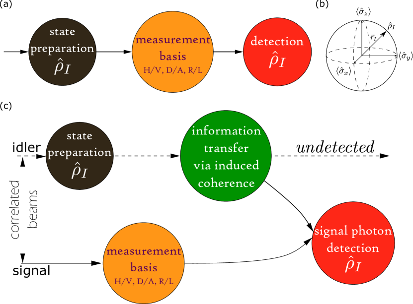
Figure 1: Quantum state tomography of photonic qubits. (a) An ensemble prepared in an unknown state $\hat{\rho}_{I}$ can be reconstructed by measurements in different bases. This technique is known as the quantum state tomography. The state $\hat{\rho}_{I}$ can be visualized as a point in the Bloch sphere depicted in (b). (c) The idler (top dashed line) and the signal (bottom solid line) photons form a photon pair (that can be produced via SPDC) and are employed for quantum state tomography of undetected photons. The idler is prepared in an initial state $\hat{\rho}_{I}$, which is transferred to the signal through induced coherence. The idler photon remains undetected. Single-photon interference patterns shown by the signal allow us to reconstruct the idler state $\hat{\rho}_{I}$.

The original proposal in Ref. [6] reconstructs the quantum state of the idler photon from the visibilities and the phase shift of the interference patterns recorded in succession for the horizontal and vertical polarization modes of the signal photon. Here, we demonstrate, as a side-effect of our investigation, how to record interference patterns in both orthogonal modes simultaneously. Moreover, we adapt the technique in such a way that instead of the visibility and the phase shift in a fixed basis, we measure only the visibilities in the three eigenbases of the Pauli operators. This approach is reminiscent of the standard quantum state tomography.

II.2 Stokes parameters

The Stokes parameters were introduced in 1852 [18] to describe the polarization of classical fields by using four quantities: the “zeroth” Stokes parameter $\textup{S}_{0}$ represents the total intensity of the field, while the parameters $\textup{S}_{x}$, $\textup{S}_{y}$, and $\textup{S}_{z}$ correspond to polarization measurements made in different polarization bases and are defined as

$$\textup{S}_{x}= |E_{D}|{{}^{2}}-|E_{A}|{{}^{2}},$$ (1)

$$\textup{S}_{y}= |E_{L}|{{}^{2}}-|E_{R}|{{}^{2}},$$ (2)

$$\textup{S}_{z}= |E_{H}|{{}^{2}}-|E_{V}|{{}^{2}}.$$ (3)

In these formulas, $E_{k}$ stands for the field’s amplitude associated with the polarization mode $k$, where $k$ is either a linear polarization (horizontal $H$, vertical $V$, diagonal $D$, and anti-diagonal $A$) or a circular polarization (left-circular $L$ and right-circular $R$). The total intensity does not depend on the polarization basis, and so

$$\textup{S}_{0}=|E_{D}|{{}^{2}}+|E_{A}|{{}^{2}}=|E_{L}|{{}^{2}}+|E_{R}|{{}^{2}}=|E_{H}|{{}^{2}}+|E_{V}|{{}^{2}}.$$ (4)

One can remove the dependence of the parameters $\textup{S}_{x}$, $\textup{S}_{y}$, and $\textup{S}_{z}$ on the intensity by dividing them by $\textup{S}_{0}$. The resulting normalized Stokes parameters allow for a convenient visual representation in the form of a Bloch vector $\vec{r}_{I}=(x,y,z)$, where

$$x=\textup{S}_{x}/\textup{S}_{0},\quad y=\textup{S}_{y}/\textup{S}_{0},\quad z=\textup{S}_{z}/\textup{S}_{0}.$$ (5)

The quantum counterpart of these normalized parameters is given by the mean values of Pauli operators [19, 1]. These operators read explicitly

$$\hat{\sigma}_{x}= |D\rangle\langle D|-|A\rangle\langle A|,$$ (6)

$$\hat{\sigma}_{y}= |L\rangle\langle L|-|R\rangle\langle R|,$$ (7)

$$\hat{\sigma}_{z}= |H\rangle\langle H|-|V\rangle\langle V|.$$ (8)

The mean values of Pauli operators for a given quantum state $\hat{\rho}_{I}$ coincide with the Bloch vector components as

$$x=\operatorname{Tr}(\hat{\sigma}_{x}\,\hat{\rho}_{I}),\quad y=\operatorname{Tr}(\hat{\sigma}_{y}\,\hat{\rho}_{I}),\quad z=\operatorname{Tr}(\hat{\sigma}_{z}\,\hat{\rho}_{I}).$$ (9)

The polarization quantum state can then be reconstructed from the Bloch vector $\vec{r}_{I}$ using the Bloch representation

$$\hat{\rho}_{I}=\frac{1}{2}(\mathbb{1}_{2}+\vec{r}_{I}\cdot\vec{\sigma}).$$ (10)

The set of all valid polarization states forms a ball referred to as the Bloch sphere, see Fig. 1(b). The pure quantum states are located on the surface of the Bloch sphere, while its interior is formed by mixed quantum states with the maximally mixed state in the center. We can parametrize the density matrix of a mixed polarization state in the $H/V$ basis as

$$\hat{\rho}_{I}=\begin{pmatrix}\alpha^{2}&\alpha\,\beta\,q\,e^{-i\xi}\\ \alpha\,\beta\,q\,e^{i\xi}&\beta^{2}\end{pmatrix},$$ (11)

where $\alpha^{2}+\beta^{2}=1$, $0\leq q\leq 1$, and $\alpha,\beta\geq 0$, $\xi\in[0,2\pi)$. The Bloch vector coordinates then read explicitly

$$x = 2\,\alpha\,\beta\,q\,\cos(\xi),$$ (12)

$$y = 2\,\alpha\,\beta\,q\,\sin(\xi),$$ (13)

$$z = \alpha^{2}-\beta^{2}.$$ (14)

III Pure states

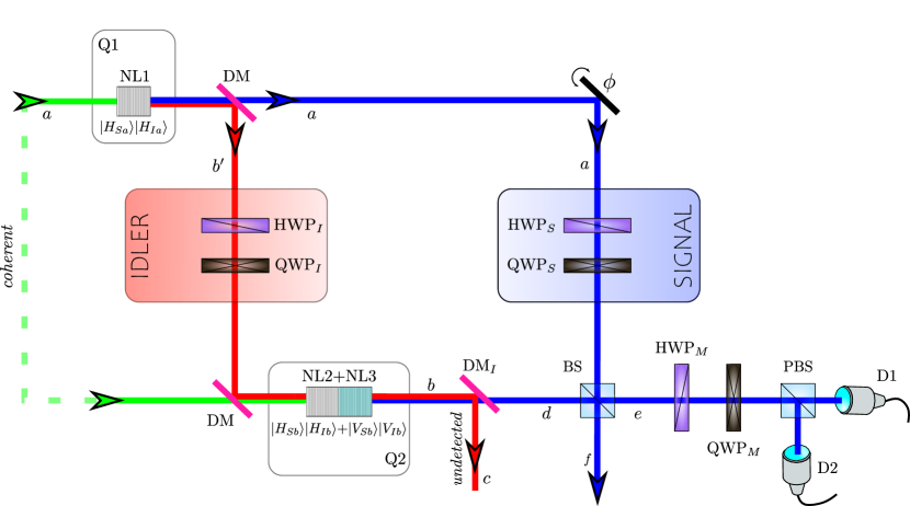
Figure 2: Imbalanced Zou-Wang-Mandel interferometer. The pump, the idler photon, and the signal photon are represented by the green, red, and blue lines, respectively. Each photon pair is created in a coherent superposition of three crystals (NL1, NL2, and NL3). Signal beams emitted from each crystal are superposed in a beam splitter (BS), and those that leave the upper port are then split into $H$ and $V$ polarization by a polarizing beam splitter (PBS) and detected by detectors D1 and D2. Idler beams are overlapped to erase the which-source information, thus, inducing coherence on the signal photon. Consequently, the intensities of the signal photon recorded by the detectors D1 and D2 exhibit interference as the independent phase $\phi$ is varied. The introduction of an additional quarter-wave plate QWP_S in the signal photon path together with half- and quarter-waveplates HWP_M and QWP_M in the detection path allows one to estimate an arbitrary polarization state of the idler photon. See the text for details. DM stands for a dichroic mirror, and HWP_I and QWP_I stand for half- and quarter-waveplates in the path of the idler photon, respectively.

We begin our discussion by considering pure quantum states of the idler photon. In what follows, we present the method of quantum state tomography of undetected photons that expands the one in Ref. [6]. Most notably, we introduce visibility Stokes parameters that represent a convenient tool for analyzing quantum measurements based on coherence. These new parameters are determined by the visibilities of the recorded interference patterns and thus complement the standard Stokes parameters based on intensities.

The physical setup of the tomography of undetected photons [6] is formed by the imbalanced Zou-Wang-Mandel (ZWM) interferometer. This interferometer, depicted in Fig. 2, consists of two sources of photon pairs, Q1 and Q2. The source Q1 produces photon pairs in a separable state $|\psi_{S}\rangle\otimes|\psi_{I}\rangle$, where $|\psi_{I}\rangle$ is the polarization state of the idler photon that is unknown to us and that we wish to reconstruct

$$|\psi_{I}\rangle=\alpha|H_{Ib^{\prime}}\rangle+\beta e^{i\xi}|V_{Ib^{\prime}}\rangle,$$ (15)

where $|k_{Ib^{\prime}}\rangle$ denotes a one-photon state of the idler photon carrying a polarization $k$ and traveling through the path $b^{\prime}$, and where $\alpha^{2}+\beta^{2}=1$, $\alpha,\beta\geq 0$, and $\xi\in[0,2\pi)$. The state of the signal photon $|\psi_{S}\rangle$ is chosen depending on the reconstruction technique and, generally, can be prepared in any pure state by including retarder plates on its path. Here, a half-wave plate HWP_S and a quarter-wave plate QWP_S are used so that the signal photon is set to

$$|\psi_{Sa}\rangle=\frac{1}{\sqrt{2}}(|H_{Sa}\rangle+e^{i\zeta}|V_{Sa}\rangle),$$ (16)

with $\zeta\in[0,2\pi)$.

The second source Q2 produces a maximally entangled state $|\Psi\rangle$ of two photons propagating along path $b$, where $|\Psi\rangle=(1/\sqrt{2})(|H_{Sb}\rangle\otimes|H_{Ib}\rangle+|V_{Sb}\rangle\otimes|V_{Ib}\rangle)$. Due to the overlap of idler beams coming from Q1 and Q2, path $b^{\prime}$ becomes $b$. This is a crucial step towards erasing the which-source information. The second step is recombining the signal beams in a beam splitter. The entire experimental setup produces a single photon pair at a time, whose state is a coherent superposition of state $|\psi_{S}\rangle\otimes|\psi_{I}\rangle$ coming from the source Q1 and $|\Psi\rangle$ coming from the source Q2. The relative pump power for sources Q1 and Q2 is chosen such that the total state of the quantum system just before the beam splitter in a lossless scenario reads

$$|\psi_{d}\rangle\propto(|H_{Sb}\rangle|H_{Ic}\rangle+|V_{Sb}\rangle|V_{Ic}\rangle)\\ +e^{i\phi}(|H_{Sa}\rangle+e^{i\zeta}|V_{Sa}\rangle)(\alpha|H_{Ic}\rangle+\beta e^{i\xi}|V_{Ic}\rangle).$$ (17)

The relevant part of the state after the beam splitter is given by

$$|\psi_{e}\rangle \propto |H_{Sb}\rangle\Bigg{(}\left(1+\alpha e^{i\phi}\right)|H_{Ic}\rangle+\beta e^{i(\phi+\xi)}|V_{Ic}\rangle\Bigg{)}$$

$$+ |V_{Sb}\rangle\Bigg{(}\alpha e^{i(\phi+\zeta)}|H_{Ic}\rangle+\left(1+\beta e^{i(\phi+\xi+\zeta)}\right)|V_{Ic}\rangle\Bigg{)}.$$

From this expression, we can obtain the analytic formulas for signal intensities and corresponding signal visibilities $\mathcal{V}$ defined as

$$\mathcal{V}=\frac{\mathcal{I}_{\textup{max}}-\mathcal{I}_{\textup{min}}}{\mathcal{I}_{\textup{max}}+\mathcal{I}_{\textup{min}}},$$ (18)

where $\mathcal{I}_{\textup{max}}$ ($\mathcal{I}_{\textup{min}}$) stands for the intensity maximum (minimum) of the signal photons. The visibilities in all three mutually unbiased bases $H/V$, $D/A$, and $L/R$ turn out to be

$$\mathcal{V}_{H}=\alpha,\quad\mathcal{V}_{V}=\beta,$$ (19)

$$\mathcal{V}_{D/A}=\frac{2\sqrt{1\pm\cos(\zeta)}}{2\pm\cos(\zeta)}\,\sqrt{\frac{1\pm 2\alpha\beta\cos(\xi)}{2}},$$ (20)

$$\mathcal{V}_{L/R}=\frac{2\sqrt{1\mp\sin(\zeta)}}{2\mp\sin(\zeta)}\,\sqrt{\frac{1\pm 2\alpha\beta\sin(\xi)}{2}}.$$ (21)

Visibilities in bases $D/A$ and $L/R$ depend on the choice of relative phase $\zeta$ in the signal photon’s state in Eq. (16). There does not exist $\zeta$ such that the prefactors in expressions (20) and (21) are both equal, but we can set $\zeta=\pi/2$ and $\zeta=0$ for the $D/A$ and $L/R$ bases, respectively, to obtain

$$\mathcal{V}_{D/A}=\sqrt{\frac{1\pm 2\alpha\beta\cos(\xi)}{2}},$$ (22)

and

$$\mathcal{V}_{L/R}=\sqrt{\frac{1\pm 2\alpha\beta\sin(\xi)}{2}}.$$ (23)

In Appendix A the general formulas for the visibilities in the three bases are shown for arbitrary pumping powers, transmission coefficients, and signal photon states. From Eqs. (19), (22), and (23) it is straightforward to check that

$$\mathcal{V}_{D}^{2}-\mathcal{V}_{A}^{2} = 2\,\alpha\beta\cos(\xi),$$ (24)

$$\mathcal{V}_{L}^{2}-\mathcal{V}_{R}^{2} = 2\,\alpha\beta\sin(\xi),$$ (25)

$$\mathcal{V}_{H}^{2}-\mathcal{V}_{V}^{2} = \alpha^{2}-\beta^{2},$$ (26)

and

$$\mathcal{V}_{D}^{2}+\mathcal{V}_{A}^{2}=1,\quad\mathcal{V}_{L}^{2}+\mathcal{V}_{R}^{2}=1,\quad\mathcal{V}_{H}^{2}+\mathcal{V}_{V}^{2}=1.$$ (27)

These expressions are in the exact correspondence with Stokes parameters in Eqs. (1)–(3) if we identify

$$\mathcal{S}_{x} \equiv \mathcal{V}_{D}^{2}-\mathcal{V}_{A}^{2},$$ (28)

$$\mathcal{S}_{y} \equiv \mathcal{V}_{L}^{2}-\mathcal{V}_{R}^{2},$$ (29)

$$\mathcal{S}_{z} \equiv \mathcal{V}_{H}^{2}-\mathcal{V}_{V}^{2}.$$ (30)

Note that for these visibility Stokes parameters $\mathcal{S}_{x}$, $\mathcal{S}_{y}$, and $\mathcal{S}_{z}$ we use a calligraphic font to differentiate them from the standard Stokes parameters $\textup{S}_{x}$, $\textup{S}_{y}$, and $\textup{S}_{z}$. This distinction will prove important later on when discussing the mixed states. The three visibility Stokes parameters allow us to calculate the coefficients $\alpha$, $\beta$, and the phase $\xi$ of the unknown state in Eq. (15) purely from visibility measurements in different bases. For the case of pure idler states $|\psi_{I}\rangle$, the three parameters $\mathcal{S}_{x}$, $\mathcal{S}_{y}$, and $\mathcal{S}_{z}$ are equal to the three coordinates $(x,y,z)=\vec{r}_{I}$ of the Bloch vector associated with the idler photon’s state. We thus recover the Bloch representation of the idler’s polarization state in Eq. (10). This demonstrates the correspondence between the traditional direct polarization measurement and our visibility measurement of undetected photons.

Let us note that in the discussion above, we used the concept of mutually unbiased bases [20]. Namely, we can measure visibilities for both modes of basis $B$ by setting the state of the signal photon such that it belongs to a basis $B^{\prime}$ that is unbiased to $B$. For example, to measure simultaneously both visibilities $\alpha$ and $\beta$ in $H/V$ basis, see Eq. (19), we have to set the signal photon into the state in Eq. (16), which is mutually unbiased with $|H_{Sa}\rangle$ and $|V_{Sa}\rangle$.

IV Mixed states

So far, we have considered only pure polarization states of the idler photon. For our tomography technique to be applicable in a practical setting, we present in this section its generalization for mixed states. At first, we present a derivation of the detection probabilities in different measurement bases of the signal photon when the idler photon is in a mixed state. Based on that, we observe that the imbalanced ZWM interferometer in Fig. 2 allows for the identification of both pure and mixed states only with some prior knowledge of the environment. When the environmental conditions are completely unknown, the uncertainty in the reconstruction of mixed states increases with the decoherence in the systems. Then, we derive the visibilities of the obtained interference patterns and define visibility Stokes parameters for mixed states with the aim of being as close as possible to the standard Stokes parameters. Finally, we discuss what assumptions about the setup can be made to enable the mixed state reconstruction in the imbalanced ZWM interferometer.

IV.1 Modelling mixed states with pure states

Mixed states can be represented as pure states living in a larger Hilbert space using a mathematical trick known as purification [1], where a given mixed state $\rho=\sum_{j}p_{j}|\varphi_{j}\rangle\langle\varphi_{j}|$ is associated with a pure state $|\psi\rangle=\sum_{j}\sqrt{p_{j}}|\varphi_{j}\rangle|a_{j}\rangle$, while $\{|a_{j}\rangle\}_{j}$ form an orthonormal basis of an extra ancillary Hilbert space. The partial trace over this extra space then gives the original mixed state as $\rho=\mathrm{Tr}_{A}(|\psi\rangle\langle\psi|)$. The choice of $\{|a_{j}\rangle\}_{j}$ is arbitrary, and any orthonormal basis will do. In the following, we adopt a more physics-inspired approach that bears some similarity to the purification yet shows important differences.

Let us assume without loss of generality that the mixed state $\hat{\rho}_{I}$ of the idler photon results from some decoherence processes in the state-preparation stage, which processes act unitarily on the composite pure state $(\alpha|H\rangle+\beta|V\rangle)\otimes|e\rangle$. Ket $|e\rangle$ denotes the pure state of all the other degrees of freedom of a photon, which we from now on collectively refer to as the environment. The decoherence processes might be polarization-dependent, and so the final state of the idler photon just before entering Q2 attains the form

$$|\psi_{I}\rangle=\alpha|H_{b^{\prime}}\rangle\otimes|e_{H}\rangle+\beta e^{i\,\xi}|V_{b^{\prime}}\rangle\otimes|e_{V}\rangle,$$ (31)

where $|e_{H}\rangle$ and $|e_{V}\rangle$ are the final states of the environment for the $|H\rangle$ and $|V\rangle$ idler photon polarization mode, respectively. These states are not in general orthogonal, and without loss of generality, we can assume that $0\leq\langle e_{H}|e_{V}\rangle\leq 1$. If we make the following identification

$$q=\langle e_{H}|e_{V}\rangle$$ (32)

it is straightforward to verify that the partial trace over the environment returns the desired mixed state

$$\hat{\rho}_{I} = \operatorname{Tr}_{e}(|\psi_{I}\rangle\langle\psi_{I}|).$$ (33)

The parameter $q$ in the parametrization of $\hat{\rho}_{I}$ in Eq. (11) quantifies the degree of coherence of the state in the $H/V$ basis: for $q=1$, the state is pure, and for $q=0$ it is completely dephased (in the $H/V$ basis). Note that, unlike the standard purification procedure, here, the states $|e_{j}\rangle$ are manifestly not orthogonal. However, there is still large freedom in their choice as $q=\langle e_{H}|e_{V}\rangle=\langle e_{H}|U^{\dagger}U|e_{V}\rangle$ for any unitary $U$. We can thus model a mixed state $\hat{\rho}_{I}$ by $|\psi_{I}\rangle$ in Eq. (31) as long as the overlap of environmental states satisfies Eq. (32). Analogously, the composite state of the second source is now

$$|\Psi\rangle=\frac{1}{\sqrt{2}}(|H_{b},H_{b}\rangle+|V_{b},V_{b}\rangle)\otimes|e_{\Psi}\rangle.$$ (34)

In what follows, we present on a more abstract level the generalization of calculations done for pure states in Sec. III. The results form the stepping stone for discussing mixed state reconstruction, visibilities, and Stokes parameters later on. To account for losses in the setup, the imperfect transmission of objects encountered by the idler photon is modeled as a beam splitter in path $b^{\prime}$ with the reflection coefficient equal to $\sqrt{1-T^{2}}$ that reflects the idler photon into path $w$. The corresponding term we denote by $|\psi_{w}\rangle$. By $|\psi_{S}\rangle$ we denote the state of the signal photon created in Q1 and propagating along path $a$ after it traversed HWP_S and QWP_S, i.e., just before it enters the beam splitter BS. Similarly, by $|\psi_{I}\rangle$ we denote the state of the idler photon created in Q1 and propagating along path $b^{\prime}$ after it traversed HWP_I and QWP_I, which is now of the form of Eq. (31). This state propagates through the source Q2 unaffected and is reflected by the dichroic mirror DM_I out of the setup. The state of signal and idler photons just before the projective measurement reads

$$|\psi\rangle=\mathcal{N}\cdot\mathrm{BS}\cdot\mathrm{DM}_{I}\cdot(Te^{i\phi}|\psi_{S}\rangle\otimes|\psi_{I}\rangle\,\\ +\sqrt{1-T^{2}}\,e^{i\phi}|\psi_{S}\rangle\otimes|\psi_{w}\rangle+P\,|\Psi\rangle),$$ (35)

where $\phi$ is the relative phase between the two sources, $P$ determines the relative pump power between the first and the second source as $P^{2}$, and $\mathcal{N}$ is a normalization factor equal to $\mathcal{N}=1/\sqrt{1+P^{2}}$.

Note that the state of the idler photon has two terms. One term is $|\psi_{I}\rangle$ coming from Q1, and the other term is included in $|\Psi\rangle$ coming from Q2. Both terms are reflected off a dichroic mirror DM_I into path $c$ out of the setup. The dichroic mirror DM_I acts only on the idler state, and the beam splitter BS acts only on the signal state. We can, therefore, rewrite the above state into

$$|\psi\rangle=\mathcal{N}\,\big{(}Te^{i\phi}|\psi^{\prime}_{S}\rangle\otimes|\psi^{\prime}_{I}\rangle\\ +\sqrt{1-T^{2}}\,e^{i\phi}|\psi^{\prime}_{S}\rangle\otimes|\psi_{w}\rangle+P\,|\Psi^{\prime}\rangle\big{)},$$ (36)

where we defined $|\psi^{\prime}_{S}\rangle=\mathrm{BS}\cdot|\psi_{S}\rangle$, $|\psi^{\prime}_{I}\rangle=\mathrm{DM}_{I}\cdot|\psi_{I}\rangle$ and $|\Psi^{\prime}\rangle=\mathrm{BS}\cdot\mathrm{DM}_{I}\cdot|\Psi\rangle$. Remember that $\langle\psi_{w}|\psi^{\prime}_{I}\rangle=\langle\psi_{w}|\Psi\rangle=0$.

At this point, we subject the signal photon to projective measurements, embodied by projectors $\hat{\Pi}_{k}$ and $\hat{\Pi}_{k}^{\perp}=\mathbb{1}-\hat{\Pi}_{k}$. For a given orthonormal basis $\{|k\rangle,|k^{\perp}\rangle\}$ the two projectors are given by $\hat{\Pi}_{k}=|k_{S}\rangle\langle k_{S}|\otimes\mathbb{1}$ and $\hat{\Pi}_{k}^{\perp}=|k_{S}^{\perp}\rangle\langle k_{S}^{\perp}|\otimes\mathbb{1}$, where the identity acts on the idler photon as well as the environment. The probability of measuring $\hat{\Pi}_{k}$ for state in Eq. (36) is easily shown to be

$$\langle\psi|\hat{\Pi}_{k}\,|\psi\rangle=\mathcal{N}^{2}(c_{k}+2\,P\,T\,\mathrm{Re}(e^{-i\phi}z_{k})),$$ (37)

where we defined numerical quantities

$$c_{k} = \langle\psi^{\prime}_{S}|\hat{\Pi}_{k}|\psi^{\prime}_{S}\rangle+P^{2}\langle\Psi^{\prime}|\hat{\Pi}_{k}|\Psi^{\prime}\rangle,$$ (38)

$$z_{k} = \langle\psi^{\prime}_{S}|\otimes\langle\psi^{\prime}_{I}|\hat{\Pi}_{k}|\Psi^{\prime}\rangle.$$ (39)

Before we proceed to discuss the visibilities of these detection probabilities, let us emphasize that there is not a single term in Eq. (37) that would contain inner products of $|\psi^{\prime}_{I}\rangle$ with itself or its projections onto some subspace. For that reason, there is no term that would contain the inner product $\langle e_{H}|e_{V}\rangle$ (32), whose determination is necessary for the characterization of the mixed state $\hat{\rho}_{I}$. This observation is independent of particular forms of $|\psi^{\prime}_{S}\rangle$ and $|\Psi^{\prime}\rangle$ and is thus quite general. We, therefore, conclude with the important statement that the imbalanced ZWM interferometer in Fig. 2 does not allow for the perfect reconstruction of mixed states unless additional constraints are enforced. We come back to this problem in Sec. IV.4.

IV.2 Visibilities

In this section, we carry out the derivation of visibilities in different bases in a way analogous to that in Sec. III. When the signal photon’s polarization is measured in an orthonormal basis $\{|k\rangle,|k^{\perp}\rangle\}$, the probability of detecting $|k\rangle$ is given in Eq. (37), which profile exhibits interference as the phase $\phi$ is varied. The visibility of the emergent interference pattern is given by (see Appendix B)

$$\mathcal{V}_{k}=2\,P\,T\,\frac{|z_{k}|}{c_{k}},$$ (40)

where $c_{k}$ and $z_{k}$ are given in Eqs. (38) and (39), respectively. This expression attains a conveniently simple form when we set $P=1$ and choose the signal photon’s state $|\psi^{\prime}_{S}\rangle$ to be unbiased with both $|k\rangle$ and $|k^{\perp}\rangle$, i.e., $|\langle\psi^{\prime}_{S}|k\rangle|=|\langle\psi^{\prime}_{S}|k^{\perp}\rangle|=1/\sqrt{2}$. It reduces to (see Appendix C)

$$\mathcal{V}_{k}=T|\langle\psi^{\prime}_{I}|k^{\ast}\rangle|e_{\Psi}\rangle|,$$ (41)

where $|k^{\ast}\rangle$ is the “complex conjugate” of vector $|k\rangle$ in the sense that if $|k\rangle=V|H\rangle$ for some unitary $V$, then $|k^{\ast}\rangle=V^{\ast}|H\rangle$, where the star stands for the complex conjugation. The visibilities are thus equal to the overlap between the idler state (with its environment) and the complex conjugate basis state with environment $|e_{\Psi}\rangle$.

The squares of visibilities show interesting properties. At first, note that from Eq. (41) and the definition of $|\psi^{\prime}_{I}\rangle$ it follows that

$$\mathcal{V}_{k}^{2} = T^{2}|\langle\psi^{\prime}_{I}|k^{\ast}\rangle|e_{\Psi}\rangle|^{2}$$ (42)

$$= T^{2}\langle\psi^{\prime}_{I}|k^{\ast}\rangle|e_{\Psi}\rangle\langle e_{\Psi}|\langle k^{\ast}|\psi^{\prime}_{I}\rangle$$

$$= \langle\psi_{I}|\,\hat{\mathcal{V}}_{k}\,|\psi_{I}\rangle,$$

where we defined an operator

$$\hat{\mathcal{V}}_{k}=T^{2}(\mathrm{DM}_{I}\cdot|k^{\ast}\rangle\langle k^{\ast}|\cdot\mathrm{DM}_{I}^{\dagger})\otimes|e_{\Psi}\rangle\langle e_{\Psi}|.$$ (43)

This visibility operator deserves more attention and is further studied in Sec. V. For the other basis vector $|k^{\perp}\rangle$ we analogously obtain

$$\mathcal{V}_{k^{\perp}}^{2}=\langle\psi_{I}|\,(T^{2}(\mathbb{1}\otimes|e_{\Psi}\rangle\langle e_{\Psi}|)-\hat{\mathcal{V}}_{k})\,|\psi_{I}\rangle,$$ (44)

which evaluates to

$$\mathcal{V}_{k^{\perp}}^{2}=T^{2}(\alpha^{2}m_{H}^{2}+\beta^{2}m_{V}^{2})-\mathcal{V}_{k}^{2},$$ (45)

where we defined

$$m_{H}=|\langle e_{H}|e_{\Psi}\rangle|,\quad m_{V}=|\langle e_{V}|e_{\Psi}\rangle|.$$ (46)

These parameters quantify the coherence of the $H$ and $V$ modes of the idler state with the second source Q2 and their properties are further studied in Sec. IV.4. From the above formulas, it directly follows that the sum of visibilities for the two orthogonal vectors is constant. This constant quantifies the level of coherence between the first and the second source, and we refer to it as the zeroth visibility Stokes parameter $\mathcal{S}_{0}$, given by

$$\mathcal{S}_{0}\equiv\mathcal{V}_{k}^{2}+\mathcal{V}_{k^{\perp}}^{2}=T^{2}(\alpha^{2}m_{H}^{2}+\beta^{2}m_{V}^{2}).$$ (47)

It is easy to see that $0\leq\mathcal{S}_{0}\leq T^{2}\leq 1$. For the difference of the two visibilities, we then obtain

$$\mathcal{V}_{k}^{2}-\mathcal{V}_{k^{\perp}}^{2}=2\mathcal{V}_{k}^{2}-\mathcal{S}_{0}.$$ (48)

This expression plays a crucial role and is discussed in the next section.

For completeness, let us list the visibilities of detection probabilities for the typical choice of single-qubit bases H/V, D/A, and R/L. For these, we get $(k,k^{\ast})\in\{(H,H),(V,V),(D,D),(A,A),(L,R),(R,L)\}$ and the visibilities explicitly read

$$\mathcal{V}_{H} = T\,\alpha\,|\langle e_{H}|e_{\Psi}\rangle|,\quad\mathcal{V}_{V}=T\,\beta\,|\langle e_{V}|e_{\Psi}\rangle|,$$ (49)

$$\mathcal{V}_{D/A} = (T/\sqrt{2})|\alpha\langle e_{H}|e_{\Psi}\rangle\pm\beta e^{-i\xi}\langle e_{V}|e_{\Psi}\rangle|,$$ (50)

$$\mathcal{V}_{L/R} = (T/\sqrt{2})|\alpha\langle e_{H}|e_{\Psi}\rangle\pm i\beta e^{-i\xi}\langle e_{V}|e_{\Psi}\rangle|.$$ (51)

Compare these expressions with Eqs. (19)–(21).

IV.3 Visibility Stokes parameters

We can define the visibility Stokes parameters for mixed states in the exact same way as we did for pure states in Eqs. (28)–(30), where the visibilities are now given by Eq. (41). The visibility Stokes parameters then explicitly read

$$\mathcal{S}_{x} = T^{2}\,2\,\alpha\,\beta\,m_{H}\,m_{V}\,\cos(\xi+\Delta\varphi),$$ (52)

$$\mathcal{S}_{y} = T^{2}\,2\,\alpha\,\beta\,m_{H}\,m_{V}\,\sin(\xi+\Delta\varphi),$$ (53)

$$\mathcal{S}_{z} = T^{2}\,(\alpha^{2}\,m^{2}_{H}-\beta^{2}\,m^{2}_{V}),$$ (54)

where we defined $\Delta\varphi=\arg\left(\langle e_{H}|e_{\Psi}\rangle\right)-\arg\left(\langle e_{V}|e_{\Psi}\rangle\right)$. The transmission coefficient $T$ can be measured for a given experimental setup independently of a particular state of the idler photon, and one can thus adjust the formulas above by removing $T$. For this reason, from now on, we effectively set $T=1$.

There are a number of problems associated with these expressions. First, the coherence terms $m_{H}$ and $m_{V}$ always appear in the product with $\alpha$ and $\beta$, respectively, which precludes the determination of the values of $\alpha$ and $\beta$ alone. Second, as discussed in Sec. IV.1, these formulas explicitly depend on the environment of the second source $|e_{\Psi}\rangle$, and there is no quantity $q$ present in the formulas. These two issues together imply that a given triple of visibility Stokes parameters $(\mathcal{S}_{x},\mathcal{S}_{y},\mathcal{S}_{z})$ is consistent with many states in the standard Bloch sphere. Moreover, the environment can have many degrees of freedom, and it can happen that states $|e_{H}\rangle$ and $|e_{V}\rangle$ turn out to be orthogonal to $|e_{\Psi}\rangle$, in which case all the visibility parameters are zero: $\mathcal{S}_{x}=\mathcal{S}_{y}=\mathcal{S}_{z}=0$. We would then misinterpret our results as corresponding to the maximally mixed state, whose Bloch vector is a zero vector.

In analogy to the standard Bloch representation, we can introduce the visibility Bloch vector $\vec{\mathcal{S}}$ as the triple

$$\vec{\mathcal{S}}=(\mathcal{S}_{x},\mathcal{S}_{y},\mathcal{S}_{z}).$$ (55)

It can be checked by the direct substitution of their explicit forms in Eqs. (52)–(54) that the three parameters satisfy

$$\mathcal{S}_{x}^{2}+\mathcal{S}_{y}^{2}+\mathcal{S}_{z}^{2}=\mathcal{S}_{0}^{2}$$ (56)

and so the norm of the visibility Bloch vector is equal to the zeroth parameter: $|\vec{\mathcal{S}}|=\mathcal{S}_{0}$. An important question is how close this visibility Bloch vector is to the actual Bloch vector $\vec{r}=(x,y,z)$. It is straightforward to show from the explicit expressions in Eqs. (12)–(14) and Eqs. (52)–(54) together with the inequality in Eq. (59), discussed in the next section, that

$$(\mathcal{S}_{x}-x)^{2}+(\mathcal{S}_{y}-y)^{2}+(\mathcal{S}_{z}-z)^{2}\leq(1-\mathcal{S}_{0})^{2}$$ (57)

and so the Euclidean distance between the two vectors is bounded from above by the incoherence $1-\mathcal{S}_{0}$. All the Bloch vectors consistent with a given $\vec{\mathcal{S}}$ thus form a ball centered in $\vec{\mathcal{S}}$ with radius $1-\mathcal{S}_{0}$, as shown in Fig. 3. The ball always touches the surface of the Bloch sphere at a point that corresponds to the pure state of the form $\alpha_{E}|H\rangle+\sqrt{1-\alpha_{E}^{2}}\exp(i\xi)|V\rangle$, where $\alpha_{E}=(1/\sqrt{2})\sqrt{1+\mathcal{S}_{z}/\mathcal{S}_{0}}$ (cf. Appendix D).

Equation (56) resembles the relation $x^{2}+y^{2}+z^{2}=r^{2}$ for standard Stokes parameters, where $r\equiv|\vec{r}|$ is the norm of the Bloch vector. This norm relates to the purity $\mathscr{P}$ of the corresponding quantum state as $\mathscr{P}=(1+r^{2})/2$. For visibility Stokes parameters, such a relation does not hold. However, from Eqs. (56) and (57) one can easily show that

$$\mathscr{P}\leq(\vec{r}\cdot\vec{\mathcal{S}})+1-\mathcal{S}_{0}.$$ (58)

One can apply the Cauchy-Schwarz inequality to the inner product in this formula to find the direct relation between the purity $\mathscr{P}$ and the coherence $\mathcal{S}_{0}$. We arrive at the lower bound in the form: $\mathscr{P}\geq 1-2\mathcal{S}_{0}(1-\mathcal{S}_{0})$ as long as $\mathcal{S}_{0}\geq 1/2$ (for $\mathcal{S}_{0}<1/2$ no special lower bound on $\mathscr{P}$ applies). Analogously, one can derive that $\mathcal{S}_{0}\leq(1+r)/2$.

When the inequality (58) is understood as a constraint on varying visibility Stokes parameters while the Bloch vector $\vec{r}$ is fixed, it turns out that this inequality represents a rotational ellipsoid, see Appendix D. For a given polarization state of a photon, one can thus, in principle, obtain many visibility Bloch vectors, depending on coherence conditions, and all these vectors form an ellipsoid, see Fig. 4.

Several other algebraic properties of the visibility Stokes parameters can be found in Appendix D. In the next section, the aforementioned issues are discussed in detail, and possible solutions to the ambiguity of the visibility Stokes parameters are proposed.

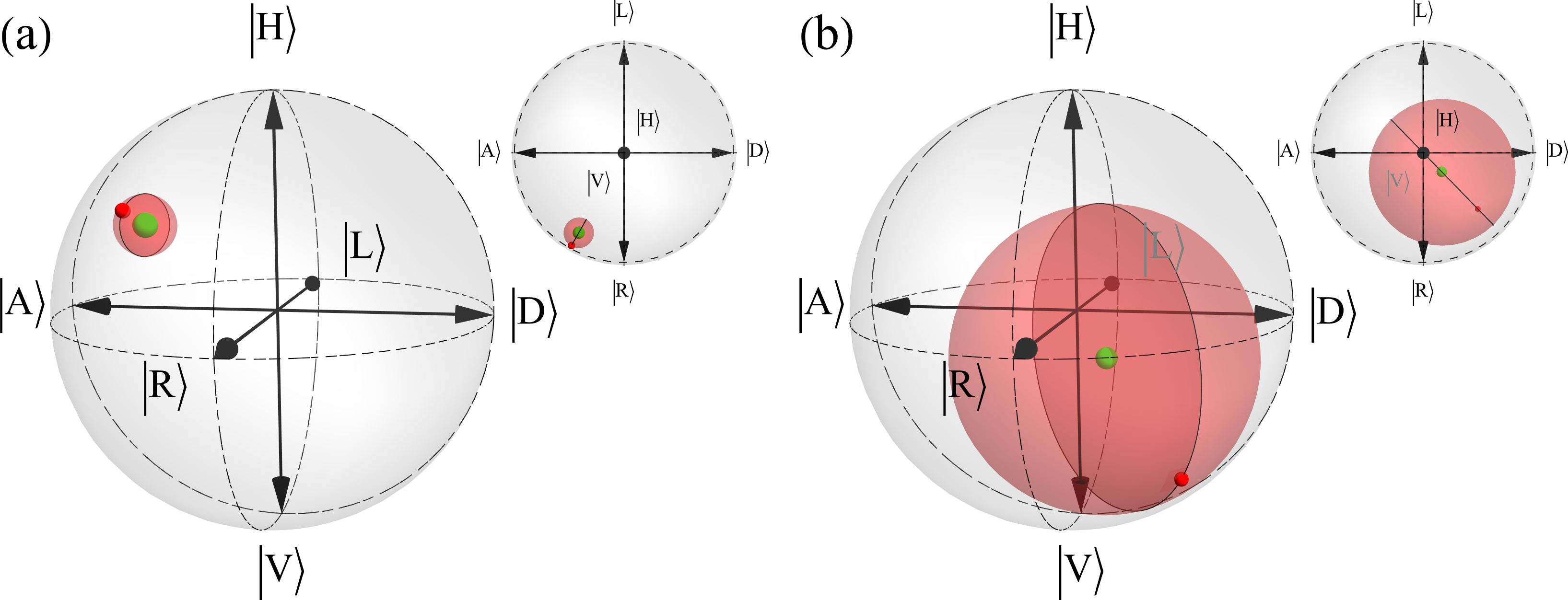
Figure 3: From visibilities to polarization states. One particular visibility Bloch vector $\vec{\mathcal{S}}$ (green dot) corresponds to many polarization states. All the standard Bloch vectors for quantum states consistent with $\vec{\mathcal{S}}$ form a ball depicted in red. This ball touches the surface of the Bloch sphere in a single point, highlighted by a red dot. (a) The side view of the Bloch sphere for $\vec{\mathcal{S}}$ with $|\vec{\mathcal{S}}|=\mathcal{S}_{0}$ close to one. The top view of the same sphere is shown in the inset. (b) For $\vec{\mathcal{S}}$ with small $\mathcal{S}_{0}$, the set of relevant states gets larger.

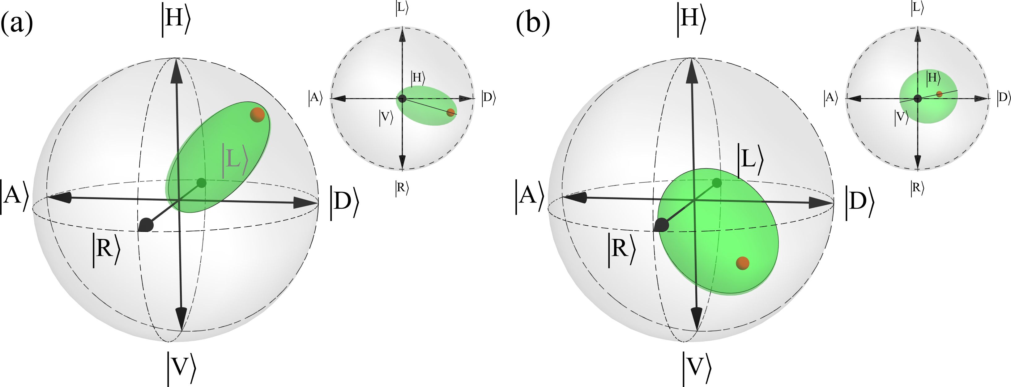
Figure 4: From polarization states to visibilities. One particular quantum state corresponds to many visibility Bloch vectors. The standard Bloch vector $\vec{r}$ of a given quantum state is represented by a red dot, while all the visibility Bloch vectors that are consistent with the state form an ellipsoid depicted in green. (a) The side view of the Bloch sphere for an almost pure polarization state. The top view of the same sphere is shown in the inset. (b) For increasingly more mixed states, the ellipsoid occupies an increasingly larger volume.

IV.4 Role of asymmetric coherence

The quantities $q$, $m_{H}$, $m_{V}$, and $\Delta\varphi$ defined in the previous section are not completely independent of each other. As shown in Appendix E, they have to satisfy inequality

$$1-\left(q^{2}+m_{H}^{2}+m_{V}^{2}\right)+2\,q\,m_{H}\,m_{V}\cos(\Delta\varphi)\geq 0,$$ (59)

where additionally $0\leq q\leq 1$, $0\leq m_{H}\leq 1$, and $0\leq m_{V}\leq 1$. The inequality (59) embodies a certain type of transitivity of coherence: when any two of the coherence parameters are close to unity, say $m_{H}$ and $m_{V}$, the third parameter, $q$, has to be almost unity as well. In terms of polarization modes and the physical setup in Fig. 2: when $H$ polarization mode from Q1 is highly coherent with $H$ produced by Q2 and also $V$ mode from Q1 is highly coherent with $V$ produced by Q2, then due to the fact that NL2 and NL3 in Q2 are highly coherent with each other, also the two polarization modes $H$ and $V$ from Q1 are highly coherent with each other. The region of valid values of $q$, $m_{H}$, and $m_{V}$ while $\Delta\varphi=0$ is plotted in Fig. 5. It is obvious from Eq. (59) that the regions for nonzero $\Delta\varphi$ are subsets of the region in Fig. 5.

As is evident from Fig. 5, for large enough values of $m_{H}$ and $m_{V}$, only a subset of values of $q$ can be attained. The whole range of $q$ from 0 to 1 is accessible only when $0\leq m_{H}=m_{V}\leq 1/\sqrt{2}$. This subset of values is depicted as a dim gray dashed line in Fig. 5. In all the other cases, the inequality (59) restricts the range of input states $\hat{\rho}_{I}$ that are consistent with the measured visibilities. For example, when both $m_{H}$ and $m_{V}$ are equal to 1, the only allowed value for $q$ is also 1. In such a case, only pure states of the idler photon can give rise to the measured visibilities.

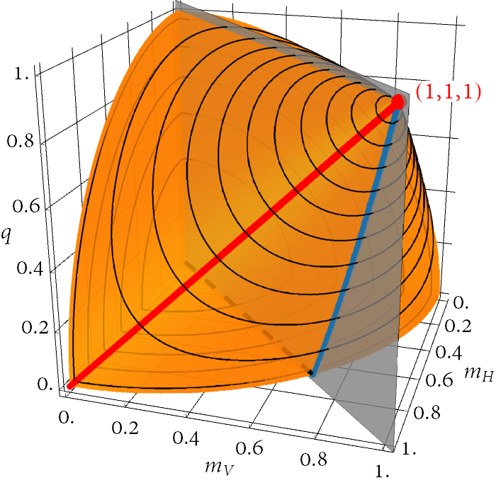
Figure 5: Region plot of valid values of coherence parameters when $\Delta\varphi=0$. The orange solid corresponds to values that satisfy inequality (59). The black contours mark the equipotential curves with $q^{2}+m_{H}^{2}+m_{V}^{2}=const.$, and the gray plane marks the constraint $m_{H}=m_{V}$. The role of all three parameters is symmetric. As the value of any of the parameters gets close to one, the region of allowed values for the other two gets smaller. The extreme point, depicted as a red dot, is when all coherence parameters attain the value of one. The red line corresponds to the allowed values of $q$ and $m_{V}$ when $m_{H}$ is set to 1. The blue line corresponds to the case when $m_{H}=m_{V}=\sqrt{(1+q)/2}$. The dashed dim line corresponds to $m_{H}=m_{V}\leq 1/\sqrt{2}$, for which the parameter $q$ can take on any value between 0 and 1. For details, see the main text.

In the general case, when the form of the interaction between the idler photon and the environment is not known, one cannot precisely reconstruct the state of the idler photon. Nevertheless, when we make some physically motivated assumptions on the interactions between the polarization and the environment, we can acquire enough information to reconstruct the mixed state $\hat{\rho}_{I}$. In the simplest scenario, when there is no interaction, we can set $|e_{H}\rangle=|e_{V}\rangle=|e_{\Psi}\rangle$ and factor the environment out of the state in Eq. (31). As a result, the state of the idler photon’s polarization is pure, and we recover the results of the previous sections. This scenario is depicted as a red dot in Fig. 5.

Another notable situation is when only the vertical polarization interacts with the environment. In contrast, the horizontal polarization is not affected, as is the case in some birefringent materials, and so $|e_{H}\rangle=|e_{\Psi}\rangle$ with $m_{H}=1$. For such values, the inequality (59) can be satisfied only when $m_{V}=q$ and $\Delta\varphi=0$. This situation is depicted as a red line in Fig. 5. Assuming that $T=1$, the visibility Stokes parameters in Eqs. (47) and (52)–(54) reduce to

$$\mathcal{S}_{x} = 2\,\alpha\,\beta\,q\,\cos(\xi),$$ (60)

$$\mathcal{S}_{y} = 2\,\alpha\,\beta\,q\,\sin(\xi),$$ (61)

$$\mathcal{S}_{z} = \alpha^{2}-(\beta\,q)^{2},$$ (62)

$$\mathcal{S}_{0} = \alpha^{2}+(\beta\,q)^{2}.$$ (63)

The first two formulas are identical to the real Bloch vector coordinates in Eqs. (12) and (13). The third formula does not match the $z$-coordinate in Eq. (14), but we can remedy this easily by noting that due to the normalization $\alpha^{2}+\beta^{2}=1$, the $z$-coordinate is equal to

$$z=\alpha^{2}-\beta^{2}=2\alpha^{2}-1=\mathcal{S}_{z}+\mathcal{S}_{0}-1.$$ (64)

In this scenario, we can thus reconstruct the polarization state of the idler photon. This special case was considered in Ref. [6], where the constraint $m_{H}=1$ was enforced by the calibration of the setup performed before the tomography itself. Obviously, when $m_{V}=1$, then analogously $q=m_{H}$ and a similar discussion can be made.

The last special case we discuss here is when the interaction between the polarization and the environment is symmetric. Specifically, when the state $|e_{H}\rangle$ deviates from $|e_{\Psi}\rangle$ in exactly the opposite fashion to the state $|e_{V}\rangle$. As a result, it holds that (cf. Appendix E)

$$|e_{\Psi}\rangle=\frac{1}{\sqrt{2(1+q)}}(|e_{H}\rangle+|e_{V}\rangle).$$ (65)

From there we obtain $m_{H}=m_{V}=\sqrt{(1+q)/2}$ and $\Delta\varphi=0$ and (provided that $T=1$) the visibility parameters read

$$\mathcal{S}_{x} = \frac{1+q}{2}\,2\,\alpha\,\beta\,\cos(\xi),$$ (66)

$$\mathcal{S}_{y} = \frac{1+q}{2}\,2\,\alpha\,\beta\,\sin(\xi),$$ (67)

$$\mathcal{S}_{z} = \frac{1+q}{2}\,(\alpha^{2}-\beta^{2}).$$ (68)

Without any adjustments, we would misinterpret our state as being depolarized by a factor of $(1+q)/2$. In contrast to the most general case of equations (52), (53), and (54) though, in the present case, we can determine the value of $q$. The zeroth visibility parameter reads

$$\mathcal{S}_{0} = \frac{1+q}{2},$$ (69)

from where we calculate $q$. At this point, we can renormalize expressions (66), (67), and (68) by dividing by $\mathcal{S}_{0}$ and multiplying by $q$ to obtain the real Bloch coordinates of the mixed state $\hat{\rho}_{I}$ in Eq.  (11). This scenario is depicted as a blue line in Fig. 5.

V Measurement operators corresponding to visibility measurements

The standard Stokes parameters can be expressed as expectation values of measurement operators in a given quantum state. In this section, we analogously introduce the operators corresponding to the visibility Stokes parameters. As follows from Eq. (42), one can express the visibilities as expectation values of specific measurement operators defined in Eq. (43). These can be used to introduce operators that correspond to the visibility Stokes parameters

$$\hat{\mathcal{S}}_{x} \equiv \hat{\mathcal{V}}_{D}-\hat{\mathcal{V}}_{A},$$ (70)

$$\hat{\mathcal{S}}_{y} \equiv \hat{\mathcal{V}}_{L}-\hat{\mathcal{V}}_{R},$$ (71)

$$\hat{\mathcal{S}}_{z} \equiv \hat{\mathcal{V}}_{H}-\hat{\mathcal{V}}_{V}.$$ (72)

All of these are Hermitian operators whose form is independent of the idler state $|\psi_{I}\rangle$. When expressed explicitly, their form turns out to be a tensor product of Pauli matrices and the projector on the state of the second source’s environment:

$$\hat{\mathcal{S}}_{x} = T^{2}(|D_{b^{\prime}}\rangle\langle D_{b^{\prime}}|-|A_{b^{\prime}}\rangle\langle A_{b^{\prime}}|)\otimes|e_{\Psi}\rangle\langle e_{\Psi}|,$$ (73)

$$\hat{\mathcal{S}}_{y} = T^{2}(|L_{b^{\prime}}\rangle\langle L_{b^{\prime}}|-|R_{b^{\prime}}\rangle\langle R_{b^{\prime}}|)\otimes|e_{\Psi}\rangle\langle e_{\Psi}|,$$ (74)

$$\hat{\mathcal{S}}_{z} = T^{2}(|H_{b^{\prime}}\rangle\langle H_{b^{\prime}}|-|V_{b^{\prime}}\rangle\langle V_{b^{\prime}}|)\otimes|e_{\Psi}\rangle\langle e_{\Psi}|.$$ (75)

These operators act on the idler polarization state together with its environment. From Eq. (42) it follows that the visibility Stokes parameters (cf. Eqs. (28)–(30)) coincide with the expectation values of the operators in Eqs. (70)–(72) as

$$\mathcal{S}_{x} = \langle\psi_{I}|\ \hat{\mathcal{S}}_{x}\ |\psi_{I}\rangle,$$ (76)

$$\mathcal{S}_{y} = \langle\psi_{I}|\ \hat{\mathcal{S}}_{y}\ |\psi_{I}\rangle,$$ (77)

$$\mathcal{S}_{z} = \langle\psi_{I}|\ \hat{\mathcal{S}}_{z}\ |\psi_{I}\rangle.$$ (78)

We have just shown how the visibility measurements that are physically performed on signal photons are expressed as measurement operators acting on the undetected idler photon. The fact that this is possible shows how information about the undetected idler photon is accessible without detecting it. The measurement operator associated with the zeroth visibility parameter $\mathcal{S}_{0}$ reads

$$\hat{\mathcal{S}}_{0}=T^{2}(\mathbb{1}\otimes|e_{\Psi}\rangle\langle e_{\Psi}|).$$ (79)

In the standard tomography, this operator is equal to the identity and does not provide us with any additional information. In our case, though, the expectation value of this operator contains information about the coherence between the idler state and the state of the second source.

Even though the operators $\hat{\mathcal{S}}_{x}$, $\hat{\mathcal{S}}_{y}$, and $\hat{\mathcal{S}}_{z}$ derived above resemble the Pauli operators in Eqs. (6)–(8), it is important to emphasize that they do not form a complete measurement in the usual sense. Formally speaking, each visibility Stokes operator $\hat{\mathcal{S}}_{k}$ corresponds to two positive measurement operators $\hat{\mathcal{V}}_{k}$ and $\hat{\mathcal{V}}_{k^{\perp}}$. These two operators nevertheless do not satisfy the completeness relation $\sum_{k}\hat{\mathcal{V}}_{k}=\mathbb{1}$. Instead, they sum up to $\mathcal{S}_{0}$, cf. Eq. (47). This can be remedied by expanding each set of visibility operators with an operator $\hat{\mathcal{V}}_{\mathrm{incoh}}\equiv\mathbb{1}-\hat{\mathcal{S}}_{0}$, quantifying the incoherence between the two sources. Unlike the standard polarization measurement, where e.g. $\hat{\Pi}_{H}+\hat{\Pi}_{V}=\mathbb{1}$ with $\hat{\Pi}_{k}=|k\rangle\langle k|$, here we have $\hat{\mathcal{V}}_{H}+\hat{\mathcal{V}}_{V}+\hat{\mathcal{V}}_{\mathrm{incoh}}=\mathbb{1}$. Let us note that for $T=1$, the visibility operators, including $\hat{\mathcal{V}}_{\mathrm{incoh}}$ are projectors.

VI Post-measurement states

In this section, we briefly discuss the post-measurement state of the idler photon alone. Let us treat for simplicity only pure polarization states $|\psi_{Ib^{\prime}}\rangle$ (15), in which case the pre-measurement state $|\psi\rangle$ (36) can be rewritten into

$$|\psi\rangle \propto Te^{i\phi}(\mathrm{BS}|\psi_{Sa}\rangle)\otimes|\psi^{\prime}_{I}\rangle$$ (80)

$$+ \sqrt{1-T^{2}}\,e^{i\phi}(\mathrm{BS}|\psi_{Sa}\rangle)\otimes|\psi_{w}\rangle$$

$$+ \frac{P}{\sqrt{2}}\,(\mathrm{BS}|H_{Sb}\rangle)\otimes(\mathrm{DM}_{I}|H_{I}\rangle)$$

$$+ \frac{P}{\sqrt{2}}\,(\mathrm{BS}|V_{Sb}\rangle)\otimes(\mathrm{DM}_{I}|V_{I}\rangle).$$

Vectors associated with different paths, $a$ and $b$, are orthogonal to each other and so $\langle\psi_{Sa}|H_{Sb}\rangle=\langle\psi_{Sa}|V_{Sb}\rangle=0$. Since both the beam splitter and the dichroic mirror are unitary operations, they do not change the orthogonality of vectors, and it is, therefore, not hard to perform a partial trace of the expression above to get the reduced state of the idler photon. We obtain

$$\hat{\rho}_{I}^{\mathrm{post}} = \operatorname{Tr}_{S}(|\psi\rangle\langle\psi|)$$ (81)

$$= \frac{T^{2}}{1+P^{2}}|\psi^{\prime}_{I}\rangle\langle\psi^{\prime}_{I}|+\frac{P^{2}}{1+P^{2}}\left(\mathbb{1}/2\right)+W,$$

where

$$W = \frac{1-T^{2}}{1+P^{2}}|\psi_{w}\rangle\langle\psi_{w}|$$ (82)

$$+ \frac{T\sqrt{1-T^{2}}}{1+P^{2}}\left(|\psi^{\prime}_{I}\rangle\langle\psi_{w}|+|\psi_{w}\rangle\langle\psi^{\prime}_{I}|\right)$$

is that part of the state that ends up in path $w$. When the transmission of the setup is perfect, and $P=1$, the final state of the idler photon reads

$$\hat{\rho}_{I}^{\mathrm{post}} = \frac{1}{2}|\psi^{\prime}_{I}\rangle\langle\psi^{\prime}_{I}|+\frac{1}{2}\left(\mathbb{1}/2\right).$$ (83)

The final state is a uniform mixture of the maximally mixed state $\mathbb{1}/2$ and the original pure state $|\psi^{\prime}_{I}\rangle$ in path $c$ (15). Evidently, the post-measurement state of the idler photon still contains some information about its original state of polarization. Also, note that the post-measurement state is not an eigenstate of a Pauli matrix as one would expect in the standard polarization tomography.

VII Conclusion

We develop the formalism of visibility Stokes parameters that complements the standard Stokes parameters in the context of coherence-based quantum operations. Specifically, we focus on the technique of quantum state tomography of undetected photons introduced in Ref. [6]. The visibility Stokes parameters characterize a quantum system that is not directly measured but whose state information can be extracted via quantum interference using the effect of induced coherence without induced emission [2]. This methodology thus profoundly differs from the standard intensity measurements for state reconstruction. The visibility Stokes parameters and the corresponding visibility operators go beyond the problem of quantum state tomography and constitute a bedrock for other quantum information techniques. These operators could enable the translation of single-photon protocols such as the BB84 [21] and the B92 [22] to the realm of optical coherence.

The form of the visibility Stokes parameters is similar to the standard Stokes parameters. Still unlike the latter, which are based on intensity measurements, the former are determined through coherence measurements in the form of visibilities. For the general case of mixed states, there are several relations between the Stokes parameters and their visibility counterparts. In general, a given triple of visibility Stokes parameters can be consistent with many polarization states of the idler photon. Similarly, many triples of visibility Stokes parameters may represent a single polarization state. We discuss possible ways to eliminate this ambiguity and establish a one-to-one relation between the standard and the visibility Stokes parameters.

To analyze the dependence of visibility Stokes parameters on the input state and the physical setup, we thoroughly analyze the environment of the idler photon. The overlap of states of environment for the first and the second source in the setup models the mixedness of the idler photon’s state and the mutual coherence between the sources. In this discussion, we assume that the two crystals composing the second source are perfectly coherent and produce a Bell pair of polarization. One could expand this discussion and study the effects of partially coherent crystals. In addition, the concept of mutually unbiased bases is applied to find an efficient implementation of the quantum tomography of undetected photons. This way, not only the form of the resulting formulas is simplified, but one can also monitor counts simultaneously in both outputs in the actual physical setup, not just one as done in Ref. [6].

In conclusion, we introduce a set of quantities akin to the standard Stokes parameters but for quantum systems composed of undetected photons. Whether there are other visibility parameters for other quantum entities remains open. The question of generalizing our results to higher dimensions is left open as well. With this, we expect to pave the way for adapting more state estimation techniques and quantum information protocols for undetected photonic systems.

VIII Acknowledgement

The authors would like to thank Armin Hochrainer and Mayukh Lahiri for fruitful discussions. J.K. thanks Prof. P. Walther for his hospitality. The financial support by the Austrian Federal Ministry of Labour and Economy, the National Foundation for Research, Technology and Development and the Christian Doppler Research Association is gratefully acknowledged.

Appendix A Visibilities for pure states

For completeness, in the following we present the general formulas for visibilities in bases $H/V$, $D/A$, and $L/R$, when the relative phase between the two crystals in the second source is equal to $\theta$ (throughout the text we could assume $\theta=0$ due to the phase calibration), the transmission in the idler photon path is $T$, and the state of the signal photon is of the form

$$|\psi_{Sa}\rangle=\delta|H_{Sa}\rangle+\varepsilon e^{i\zeta}|V_{Sa}\rangle,$$ (84)

where $\delta^{2}+\varepsilon^{2}=1$, $\delta,\varepsilon\geq 0$ and $\zeta\in[0,2\pi)$. Moreover, let the relative pump power between the first and the second source be equal to $P^{2}$, where $P$ is a real number. In such a general case the visibilities are given by

$$\mathcal{V}_{H}=\frac{2\sqrt{2}\delta PT}{P^{2}+2\delta^{2}}\,\alpha, \mathcal{V}_{V}=\frac{2\sqrt{2}\varepsilon PT}{P^{2}+2\varepsilon^{2}}\,\beta,$$

$$\mathcal{V}_{D/A}=\frac{2PT\sqrt{1\pm 2\delta\varepsilon\cos(\zeta)}}{1+P^{2}\pm 2\delta\varepsilon\cos(\zeta)}\,\sqrt{\frac{1\pm 2\alpha\beta\cos(\xi-\theta)}{2}},$$

$$\mathcal{V}_{L/R}=\frac{2PT\sqrt{1\mp 2\delta\varepsilon\sin(\zeta)}}{1+P^{2}\mp 2\delta\varepsilon\sin(\zeta)}\,\sqrt{\frac{1\pm 2\alpha\beta\sin(\xi-\theta)}{2}}.$$

We recover the formulas (19)–(21) from these general expressions for $T=1$, $P=1$, $\theta=0$ and $\delta=\varepsilon=1/\sqrt{2}$.

Appendix B Visibilities for mixed states

The formula for the detection probability in Eq. (37) can be recast into

$$\langle\psi|\hat{\Pi}_{j}\,|\psi\rangle=2\,P\,T\mathcal{N}^{2}\,\mathrm{Re}(z_{j})\cos(\phi)\\ +2\,P\,T\mathcal{N}^{2}\,\mathrm{Im}(z_{j})\sin(\phi)+\mathcal{N}^{2}c_{j},$$ (85)

which is of the form $f(\phi)=A\cos(\phi)+B\sin{(\phi)}+C$ for real constants $A$, $B$, and $C$. One can always find a non-negative $D$ and real $\omega$ such that $A=D\sin(\omega)$ and $B=D\cos(\omega)$. The original expression can then be rewritten into $f(\phi)=C+D\sin(\phi+\omega)$, from which it is evident that the visibility is equal to $D/C$. Since $A^{2}+B^{2}=D^{2}$ we get that the visibility equals $\sqrt{A^{2}+B^{2}}/C$. When we plug the explicit forms of $A$, $B$, and $C$ into this formula, we obtain the expression in Eq. (40).

Appendix C Visibilities for unbiased signal states

In this section we derive the form of visibilities in Eq. (41) from the general formula in Eq. (40). First, note that the state produced by the second source, Eq. (34), is the tensor product of the Bell state $|\Phi^{+}\rangle$ and the environmental state $|e_{\Psi}\rangle$. The Bell state exhibits a unitary invariance of the form $U\otimes U^{\ast}|\Phi^{+}\rangle=|\Phi^{+}\rangle$ for an arbitrary one-qubit unitary $U$ and its complex conjugate $U^{\ast}$. If one projects the first qubit on state $|k\rangle$, the post-measurement state of the second qubit reads

$$\langle k|\Phi^{+}\rangle =\langle H|(V^{\dagger}\otimes\mathbb{1})|\Phi^{+}\rangle$$

$$=\langle H|(\mathbb{1}\otimes V^{\ast})(V^{\dagger}\otimes V^{T})|\Phi^{+}\rangle$$

$$=\langle H|(\mathbb{1}\otimes V^{\ast})|\Phi^{+}\rangle$$

$$=(1/\sqrt{2})V^{\ast}|H\rangle,$$ (86)

where $|k\rangle=V|H\rangle$ for a specific unitary $V$, and where we used the unitary invariance for $U=V^{\dagger}$.

We model the symmetric beam splitter by a Hadamard matrix. If we fix the projector $\hat{\Pi}_{j}$ to act on path $b$, it is easy to show that the brakets in the definition of $c_{j}$ in Eq. (38) reduce to $\langle\psi^{\prime}_{S}|\hat{\Pi}_{j}|\psi^{\prime}_{S}\rangle=\langle\psi_{S}|\mathrm{BS}^{\dagger}\hat{\Pi}_{j}\mathrm{BS}|\psi_{S}\rangle=(1/2)\langle\psi_{S}|\hat{\Pi}_{j}|\psi_{S}\rangle$ and $\langle\Psi^{\prime}|\hat{\Pi}_{j}|\Psi^{\prime}\rangle=\langle\Phi^{+}|\mathrm{BS}^{\dagger}\hat{\Pi}_{j}\mathrm{BS}|\Phi^{+}\rangle=(1/2)\langle\Phi^{+}|\hat{\Pi}_{j}|\Phi^{+}\rangle$. Similarly, $z_{j}$ in Eq. (39) reduces to $\langle\psi^{\prime}_{S}|\otimes\langle\psi^{\prime}_{I}|\hat{\Pi}_{j}|\Psi^{\prime}\rangle=\langle\psi_{S}|\mathrm{BS}^{\dagger}\hat{\Pi}_{j}\mathrm{BS}\otimes\langle\psi_{I}|\Psi\rangle=(-1/2)\langle\psi_{S}|\hat{\Pi}_{j}\otimes\langle\psi_{I}|\Psi\rangle$.

From Eq. (86) we further get $\langle\Phi^{+}|\hat{\Pi}_{j}|\Phi^{+}\rangle=\langle\Phi^{+}|j\rangle\langle j|\Phi^{+}\rangle=1/2$. As mentioned in the main text, we set the signal’s state $|\psi_{S}\rangle$ to be mutually unbiased with the projection vector $|j\rangle$, where $\hat{\Pi}_{j}=|j\rangle\langle j|$, that is $\langle\psi_{S}|j\rangle=(1/\sqrt{2})\exp(i\varphi_{j})$ for some real $\varphi_{j}$. From there it follows that $\langle\psi_{S}|\hat{\Pi}_{j}|\psi_{S}\rangle=1/2$ and $\langle\psi_{S}|\hat{\Pi}_{j}\otimes\langle\psi_{I}|\Psi\rangle=(1/\sqrt{2})\exp(i\varphi_{j})\langle j|\langle\psi_{I}|\Phi^{+}\rangle|e_{\Psi}\rangle=(1/2)\exp(i\varphi_{j})\langle\psi_{I}|V_{j}^{\ast}|H\rangle|e_{\Psi}\rangle$, where $|j\rangle=V_{j}|H\rangle$ and where we used Eq. (86).

Taken all these simplifications into account, we can recast the form of $c_{j}$ and $|z_{j}|$ into $c_{j}=(1/4)(1+P^{2})$ and $|z_{j}|=(1/4)|\langle\psi_{I}|j^{\ast}\rangle|e_{\Psi}\rangle|$, where we define $|j^{\ast}\rangle=V_{j}^{\ast}|H\rangle$. The ratio of these two quantities determines the visibility, for which we obtain

$$\mathcal{V}_{j}=2\,P\,T\frac{|\langle\psi_{I}|j^{\ast}\rangle|e_{\Psi}\rangle|}{1+P^{2}}.$$ (87)

As is easy to see, when setting $P=1$, this formula reduces to Eq. (41) as we wanted to show.

Appendix D Relations of visibility Stokes parameters

The quantum states are normalized such that the standard zeroth Stokes parameter is always unity for both pure and mixed states. If we follow the same logic and divide all the parameters in Eqs. (52)–(54) as well as $\mathcal{S}_{0}$ in Eq. (47) by $\mathcal{S}_{0}$, provided that $\mathcal{S}_{0}\neq 0$, these turn into

$$\overline{\mathcal{S}_{x}}\equiv\mathcal{S}_{x}/\mathcal{S}_{0} = 2\,\overline{\alpha}\,\overline{\beta}\,\cos(\overline{\xi}),$$ (88)

$$\overline{\mathcal{S}_{y}}\equiv\mathcal{S}_{y}/\mathcal{S}_{0} = 2\,\overline{\alpha}\,\overline{\beta}\,\sin(\overline{\xi}),$$ (89)

$$\overline{\mathcal{S}_{z}}\equiv\mathcal{S}_{z}/\mathcal{S}_{0} = \overline{\alpha}^{2}-\overline{\beta}^{2},$$ (90)

$$\overline{\mathcal{S}_{0}}\equiv\mathcal{S}_{0}/\mathcal{S}_{0} = 1,$$ (91)

where $(\overline{\alpha},\overline{\beta})$ is a unit vector with

$$\overline{\alpha} = \frac{\alpha\,m_{H}}{\sqrt{\alpha^{2}\,m^{2}_{H}+\beta^{2}\,m^{2}_{V}}},\quad\overline{\beta}=\frac{\beta\,m_{V}}{\sqrt{\alpha^{2}\,m^{2}_{H}+\beta^{2}\,m^{2}_{V}}},$$

$$\overline{\xi} = \xi+\Delta\varphi.$$ (92)

The normalized visibility Stokes parameters in Eqs. (88)–(91) thus formally correspond to Stokes parameters of a pure state $|\overline{\psi}\rangle=\overline{\alpha}|H\rangle+\overline{\beta}\exp(i\overline{\xi})|V\rangle$. The transmission coefficient $T$ is no longer present in the normalized formulas, but the problems mentioned in the main text remain. From this discussion it is obvious that the visibility Stokes parameters do not directly hold any information about the purity of the measured state. For a given triple of (non-normalized) visibility Stokes parameters, there is exactly one pure state $|\overline{\psi}\rangle$ determined by the corresponding normalized parameters. From the normalization condition $\overline{\alpha}^{2}+\overline{\beta}^{2}=1$ and Eq. (90) it follows directly that for this state $\overline{\alpha}=(1/\sqrt{2})\sqrt{1+\mathcal{S}_{z}/\mathcal{S}_{0}}$.

It is easy to see that Eq. (58) is invariant under the simultaneous rotation of both $\vec{r}$ and $\vec{\mathcal{S}}$. We can thus rotate the coordinate system such that $\vec{r}=(r,0,0)$, upon which rotation the visibility Bloch vector turns into $(\mathcal{S}_{x}^{\prime},\mathcal{S}_{y}^{\prime},\mathcal{S}_{z}^{\prime})$. The inequality (58) then turns into

$$\mathcal{S}_{0}\leq r\mathcal{S}_{x}^{\prime}+(1-r^{2})/2$$ (93)

as the norm $\mathcal{S}_{0}$ of the visibility Stokes vector remains the same. Since $\mathcal{S}_{0}\geq 0$, both sides of this inequality are non-negative and the inequality is preserved when one takes the square of both sides. When one does it and simplifies the result, one can recast the final expression into the form

$$\frac{(\mathcal{S}_{x}^{\prime}-r/2)^{2}}{(1/2)^{2}}+\frac{(\mathcal{S}_{y}^{\prime})^{2}}{(\sqrt{1-r^{2}}/2)^{2}}+\frac{(\mathcal{S}_{z}^{\prime})^{2}}{(\sqrt{1-r^{2}}/2)^{2}}\leq 1,$$ (94)

which describes a rotational ellipsoid with its center in point $\vec{r}/2$ and with semiaxes $1/2$ and $\sqrt{1-r^{2}}/2$, while the two loci are situated in the origin $(0,0,0)$ and point $\vec{r}$. These properties are preserved when one expresses the ellipsoid in the original variables $\vec{\mathcal{S}}$.

Let us mention some neat algebraic relations for $\mathcal{S}_{0}$. Namely,

$$\mathcal{V}_{D}^{2}+\mathcal{V}_{A}^{2}+\mathcal{V}_{L}^{2}+\mathcal{V}_{R}^{2}+\mathcal{V}_{H}^{2}+\mathcal{V}_{V}^{2} =3\mathcal{S}_{0},$$ (95)

$$\mathcal{V}_{D}^{4}+\mathcal{V}_{A}^{4}+\mathcal{V}_{L}^{4}+\mathcal{V}_{R}^{4}+\mathcal{V}_{H}^{4}+\mathcal{V}_{V}^{4} =2\mathcal{S}_{0}^{2},$$ (96)

$$\mathcal{V}_{D}^{2}\mathcal{V}_{A}^{2}+\mathcal{V}_{L}^{2}\mathcal{V}_{R}^{2}+\mathcal{V}_{H}^{2}\mathcal{V}_{V}^{2} =(1/2)\mathcal{S}_{0}^{2}.$$ (97)

As the left-hand sides contain visibilities measured in all three standard bases, the value of $\mathcal{S}_{0}$ thus obtained might be less sensitive to experimental imperfections. Formula (95) follows directly from the threefold use of the definition of $\mathcal{S}_{0}$ (47). When we square both sides of Eq. (47) and analogously to Eq. (95) sum up its three versions, we arrive at

$$(\mathcal{V}_{D}^{2}+\mathcal{V}_{A}^{2})^{2}+(\mathcal{V}_{L}^{2}+\mathcal{V}_{R}^{2})^{2}+(\mathcal{V}_{H}^{2}+\mathcal{V}_{V}^{2})^{2}=3\mathcal{S}_{0}^{2}.$$ (98)

Furthermore, from Eq. (56) we get

$$(\mathcal{V}_{D}^{2}-\mathcal{V}_{A}^{2})^{2}+(\mathcal{V}_{L}^{2}-\mathcal{V}_{R}^{2})^{2}+(\mathcal{V}_{H}^{2}-\mathcal{V}_{V}^{2})^{2}=\mathcal{S}_{0}^{2}.$$ (99)

When we sum up these last two equations, we immediately obtain Eq. (96). When we instead subtract the second equation from the first, we get Eq. (97).

Appendix E Constraints on coherence parameters

The three coherence terms $q$, $m_{V}$ and $m_{V}$ are defined as scalar products of three environmental states $|e_{H}\rangle$, $|e_{V}\rangle$, and $|e_{\Psi}\rangle$ introduced in Eqs. (32) and (46). Without loss of generality we can write

$$|e_{\Psi}\rangle=\gamma_{H}|e_{H}\rangle+\gamma_{V}|e_{V}\rangle+\gamma_{\perp}|e_{\perp}\rangle$$ (100)

for some complex numbers $\gamma_{H}$, $\gamma_{V}$, and $\gamma_{\perp}$ and a vector $|e_{\perp}\rangle$, for which $\langle e_{H}|e_{\perp}\rangle=\langle e_{V}|e_{\perp}\rangle=0$. The norm of $|e_{\Psi}\rangle$ reads

$$\langle e_{\Psi}|e_{\Psi}\rangle=|\gamma_{H}|^{2}+|\gamma_{V}|^{2}+|\gamma_{\perp}|^{2}+2q\,\mathrm{Re}(\gamma_{H}^{\ast}\gamma_{V})$$ (101)

and has to be equal to unity. From this condition we get

$$|\gamma_{H}|^{2}+|\gamma_{V}|^{2}+2q\,\mathrm{Re}(\gamma_{H}^{\ast}\gamma_{V})=1-|\gamma_{\perp}|^{2}\leq 1.$$ (102)

It further holds that

$$m_{H}e^{i\varphi_{H}}\equiv\langle e_{H}|e_{\Psi}\rangle = \gamma_{H}+\gamma_{V}\,q,$$ (103)

$$m_{V}e^{i\varphi_{V}}\equiv\langle e_{V}|e_{\Psi}\rangle = \gamma_{H}\,q+\gamma_{V},$$ (104)

from where one gets

$$\gamma_{H} = (m_{H}e^{i\varphi_{H}}-q\,m_{V}e^{i\varphi_{V}})/(1-q^{2}),$$ (105)

$$\gamma_{V} = (m_{V}e^{i\varphi_{V}}-q\,m_{H}e^{i\varphi_{H}})/(1-q^{2}).$$ (106)

By plugging these expressions into the inequality (102) and simplifying the result one arrives at

$$1-\left(q^{2}+m_{H}^{2}+m_{V}^{2}\right)+2\,q\,m_{H}\,m_{V}\cos(\Delta\varphi)\geq 0$$ (107)

with $\Delta\varphi=\varphi_{H}-\varphi_{V}$, as we wanted to show. From there we further obtain the inequality

$$1-\left(q^{2}+m_{H}^{2}+m_{V}^{2}\right)+2\,q\,m_{H}\,m_{V}\geq 0,$$ (108)

which is independent of $\Delta\varphi$. This same inequality can also be derived from general considerations for density matrices, where one requires the matrix to be positive semi-definite. Similar discussion was done in the supplementary of Ref. [6]. When we identify $q$ and $m_{V}$ with the coherence parameters $\mathscr{I}$ and $\mathscr{L}$ from Ref. [6] and set $\mathscr{L}=\mathscr{L}^{\prime}$ and $m_{H}=1$, then inequality (107) can be satisfied only when $\mathscr{I}=\mathscr{L}$. Exactly this condition was also obtained in Ref. [6].

Note that the inequalities above contain only inner products of environmental states and are thus invariant under the unitary evolution acting on the environment. This way, we remove the arbitrariness in our original choice of $|e_{H}\rangle$, $|e_{V}\rangle$, and $|e_{\Psi}\rangle$.

When the environment is known to be only two-dimensional, e.g. when the environment is artificially set by an experimenter, the inequality (108) turns into a quadratic equation, which we can solve for $q$ obtaining $q_{\pm}=m_{H}m_{V}\pm\sqrt{1+m_{H}^{2}m_{V}^{2}-m_{H}^{2}-m_{V}^{2}}$. For $m_{H}=1$ (or $m_{V}=1$), the expression under the square root vanishes and we are left with a unique solution $q_{+}=q_{-}=q=m_{V}$ (or $q=m_{H}$) that allows for a perfect reconstruction of the mixed state $\hat{\rho}_{I}$. This condition was enforced in Ref. [6] and the reconstruction of pure idler state is obviously a special case of this condition with $m_{H}=m_{V}=1$. Let us recall that $q$ has to lie in the interval $[0,1]$. The “plus” solution $q_{+}$ complies with this requirement, while the “minus” solution $q_{-}$ complies as long as $m_{H}^{2}+m_{V}^{2}\geq 1$. For the region with $m_{H}^{2}+m_{V}^{2}<1$ we thus obtain a unique solution $q_{+}$. If it further holds that $m_{H}=m_{V}$, the “plus” solution reduces to $q_{+}=1$, while the “minus” solution reads $q_{-}=2m_{H}^{2}-1$ as long as $1/\sqrt{2}\leq m_{H}=m_{V}\leq 1$. This last condition is exemplified by the state in Eq. (65) in the main text.

References

• [1] Michael A. Nielsen and Isaac L. Chuang. Quantum computation and quantum information. Cambridge University Press, Cambridge; New York, 10th anniversary ed edition, 2010.
• [2] L.J. Wang, X.Y. Zou, and L. Mandel. Induced coherence without induced emission. Physical Review A, 44(7):4614, 1991.
• [3] X.Y. Zou, L. J. Wang, and L. Mandel. Induced coherence and indistinguishability in optical interference. Physical review letters, 67(3):318, 1991.
• [4] Armin Hochrainer, Mayukh Lahiri, Radek Lapkiewicz, Gabriela Barreto Lemos, and Anton Zeilinger. Quantifying the momentum correlation between two light beams by detecting one. Proc. Natl. Acad. Sci. USA, 114(7):1508–1511, 2017.
• [5] Gabriela Barreto Lemos, Radek Lapkiewicz, Armin Hochrainer, Mayukh Lahiri, and Anton Zeilinger. One-photon measurement of two-photon entanglement. Phys. Rev. Lett., 130(9):090202, 2023.
• [6] Jorge Fuenzalida, Jaroslav Kysela, Krishna Dovzhik, Gabriela Barreto Lemos, Armin Hochrainer, Mayukh Lahiri, and Anton Zeilinger. Quantum state tomography of undetected photons. Phys. Rev. A, 109(2):022413, 2024.
• [7] Jorge Fuenzalida, Enno Giese, and Markus Gräfe. Nonlinear interferometry: A new approach for imaging and sensing. Adv. Quantum Technol., page 2300353, 2024.
• [8] G. Barreto Lemos, V. Borish, G. D. Cole, S. Ramelow, R. Lapkiewicz, and A. Zeilinger. Quantum imaging with undetected photons. Nature, 512(7515):409–412, 2014.
• [9] Marta Gilaberte Basset, Armin Hochrainer, Sebastian Töpfer, Felix Riexinger, Patricia Bickert, Josué Ricardo León‐Torres, Fabian Steinlechner, and Markus Gräfe. Video‐rate imaging with undetected photons. 15(6):2000327.
• [10] D. A. Kalashnikov, A. V. Paterova, S. P. Kulik, and L. A. Krivitsky. Infrared spectroscopy with visible light. Nature Photonics, 10(2):98, 2016.
• [11] A. Vallés, G. Jiménez, L. J. Salazar-Serrano, and J. P. Torres. Optical sectioning in induced coherence tomography with frequency-entangled photons. Physical Review A, 97(2):023824, 2018.
• [12] A. V. Paterova, H. Yang, C. An, D. A. Kalashnikov, and L. A. Krivitsky. Tunable optical coherence tomography in the infrared range using visible photons. Quantum Science and Technology, 3(2):025008, 2018.
• [13] Sebastian Töpfer, Marta Gilaberte Basset, Jorge Fuenzalida, Fabian Steinlechner, Juan P Torres, and Markus Gräfe. Quantum holography with undetected light. Sci. Adv., 8(2):eabl4301, 2022.
• [14] Jorge Fuenzalida, Marta Gilaberte Basset, Sebastian Töpfer, Juan P Torres, and Markus Gräfe. Experimental quantum imaging distillation with undetected light. Sci. Adv., 9(35):eadg9573, 2023.
• [15] Armin Hochrainer, Mayukh Lahiri, Manuel Erhard, Mario Krenn, and Anton Zeilinger. Quantum indistinguishability by path identity and with undetected photons. Rev. Mod. Phys., 94:025007, Jun 2022.
• [16] Daniel F. V. James, Paul G. Kwiat, William J. Munro, and Andrew G. White. Measurement of qubits. Phys. Rev. A, 64:052312, Oct 2001.
• [17] J. B. Altepeter, E. R. Jeffrey, and P. G. Kwiat. Photonic state tomography. Advances in Atomic, Molecular, and Optical Physics, 52:105–159, 2005.
• [18] G. G. Stokes. On the composition and resolution of streams of polarized light from different sources. Transactions of the Cambridge Philosophical Society, 9:399, 1851.
• [19] Wolfgang Pauli. Zur quantenmechanik des magnetischen elektrons. Z. Physik, (43):601–623, 1927.
• [20] Thomas Durt, Berthold-Georg Englert, Ingemar Bengtsson, and Karol Życzkowski. On mutually unbiased bases. International Journal of Quantum Information, 08(04):535–640, June 2010.
• [21] Charles H. Bennett and Gilles Brassard. Quantum cryptography: Public key distribution and coin tossing. Theoretical Computer Science, 560:7–11, December 2014.
• [22] Charles H. Bennett. Quantum cryptography using any two nonorthogonal states. Physical Review Letters, 68(21):3121–3124, May 1992.