Theoretical Probes of Higgs-Axion non-perturbative Couplings

Abstract

In this work we investigate the phenomenological implications of several non-trivial axion-Higgs couplings, which cover most of the possible non-perturbative scenarios. Specifically we consider the combination of having higher order non-renormalizable Higgs-axion couplings originating from a weakly coupled effective theory combined with non-perturbative couplings of the form $\sim\epsilon\Lambda_{c}^{2}|H|^{2}\cos(\frac{\phi}{f_{a}})$. Since we consider the misalignment axion, the non-perturbative couplings can be expanded in the form of a perturbation expansion in powers of $\phi/f_{a}$, thus after the electroweak symmetry breaking, the effective potential of the axion is drastically affected by these terms. We investigate the phenomenological implications of these terms for various values of the mass scale $\Lambda_{c}$, and some scenarios are theoretically disfavored, while other scenarios with non-perturbative Higgs-axion couplings of the form $\sim\epsilon\Lambda_{c}^{2}|H|^{2}\cos(\frac{\phi}{f_{a}})$ with $\Lambda_{c}\sim 10^{-10}\times m_{a}$ and $m_{a}\sim 10^{-10}\,$eV, lead to a characteristic pattern in the stochastic gravitational wave background via the deformation of the background equation of state parameter occurring at frequencies probed by the Einstein Telescope. We also consider loop effects from the Higgs sector caused by the term $\sim\epsilon\Lambda_{c}^{2}|H|^{2}\cos(\frac{\phi}{f_{a}})$ if we close the Higgs in one loop.

I Introduction

The next decade is anticipated by most theoretical physicists since, many fundamental theories of theoretical physics will be put into test. Specifically, inflation [1, 2, 3, 4, 5], one of our cornerstone descriptions of the early Universe, will be tested by the stage 4 Cosmic Microwave Background (CMB) experiments [6, 7]. The future highly anticipated gravitational wave experiments will also shed light on the primordial era of our Universe, by detecting stochastic gravitational wave patterns [8, 9, 10, 11, 12, 13, 14, 15, 16]. The chorus of stochastic gravitational wave detections has started by the NANOGrav and other Pulsar Timing Array (PTA) collaborations in 2023 [17, 18, 19, 20]. Now, regarding the stochastic gravitational wave background, the NANOGrav 2023 signal cannot be explained by inflationary theories, unless these have an abnormal large blue-tilted tensor spectral index [21]. There exist alternative possibilities, such as low energy first order phase transitions with the transition temperature being of the order $\sim\mathcal{O}(1)\,$GeV, since a first order phase transition can generate bubble nucleation of the new vacuum which can effectively produce stochastic gravitational waves. This physical possibility applies to higher frequencies too, where the electroweak phase transition can be probed by LISA, the Einstein Telescope, the BBO and the DECIGO experiments, and a significant amount of work has been produced examining the possibility of having gravitational waves by first order phase transitions during the radiation domination era [22, 23, 24, 25, 26, 27, 28, 29, 30, 31, 32, 33, 34, 35, 36, 37, 38, 39, 40, 41, 35, 42, 43, 44]. In most of the above scenarios, singlet extensions of the Standard Model are considered, with the $SU(3)\times SU(2)\times U(1)$ singlet scalar being solely coupled with the Higgs sector [46, 47, 48, 49, 50, 51, 52, 53, 54, 55, 56, 49, 57, 58, 59, 60, 61, 62, 50, 63, 59], or in some cases, Higgs self couplings in the form of higher dimensional non-renormalizable operators [27, 30, 44] can achieve such a phase transition. Also in most of the cases, the singlet extensions of the Standard Model serve as potential dark matter candidate particles, since these scalars are perfect weakly interacting massive particles (WIMPs). However, no WIMP has been detected so far (2024), which casts some doubt on the very existence of dark matter, without of course excluding the possibility to find a WIMP in the next years, see [64] for a recent update on the WIMP scientific status. Although formal relativistic materializations of Modified Newtonian Dynamics are promising [65, 66, 67, 68], so far the dark matter mystery exists. The pessimistic scenario in which dark matter is actually a particle that belongs to a truly dark sector, completely uncoupled with the Standard Model sector, is a true possibility. In that case, it is rather hard to verify experimentally the existence of dark matter, at least in a direct way. There is also however the scenario in which the Higgs sector is weakly coupled to the dark matter particle. One strong dark matter candidate, is the elusive axion particle [69, 70, 71, 72, 73, 74, 75, 76, 77, 78, 79, 80, 81, 82, 83, 84, 85, 86, 87, 88, 89, 90, 91, 92, 93, 94, 95, 96, 97, 98, 99, 100, 101], see also [102, 103] for reviews and in addition an interesting simulation [104] for $\mu$eV range axions. The axion or some axion like particle, is expected to have a significantly small mass, and several experiments already exist targeting to detect the axion [105]. Also proposals for the axion mass have appeared in the literature [106, 107], pointing to a light axion mass of the order $m_{a}\sim\mathcal{O}(10^{-10})\,$eV, by using Gamma Ray Bursts observational data. In this work we shall consider the misalignment axion particle and we shall explore the phenomenological implications of couplings of this light particle with the Higgs sector. We shall be very cautious in choosing the couplings, since renormalizable couplings may lead to a thermalization of the axion, which is constrained by Higgs decays in the Large Hadron Collider (LHC). The misalignment axion is a non-thermal dark matter relic, so we will avoid studying renormalizable couplings of the axion to the Higgs sector. Specifically we shall consider the combination of dimension 4 and dimension 6 higher order non-renormalizable couplings to the Higgs particle and couplings of the form $\sim\epsilon\Lambda_{c}^{2}|H|^{2}\cos(\frac{\phi}{f_{a}})$ where $\epsilon$ is some constant smaller than unity, $\Lambda_{c}$ is an arbitrary scale, $H$ is the Standard Model Higgs, $\phi$ is the axion and $f_{a}$ is the axion decay constant. The effect of the simple case of having only dimension 4 and dimension 6 higher order non-renormalizable couplings to the Higgs particle was considered in Ref. [108], and in this work we extend the analysis including couplings of the form $\sim\epsilon\Lambda_{c}^{2}|H|^{2}\cos(\frac{\phi}{f_{a}})$, which were introduced in [109]. Due to the misalignment mechanism, the couplings $\sim\epsilon\Lambda_{c}^{2}|H|^{2}\cos(\frac{\phi}{f_{a}})$ can be expanded in a perturbation expansion in terms of $\frac{\phi}{f_{a}}$ and the effective potential of the axion is altered after the electroweak phase transition. As we shall see, the effects introduced by the couplings $\sim\epsilon\Lambda_{c}^{2}|H|^{2}\cos(\frac{\phi}{f_{a}})$ are dramatic phenomenologically, depending on the value of the mass scale $\Lambda_{c}$. As we demonstrate, large mass scales of the order of the Higgs mass are forbidden since they might lead to axion vacua which are energetically equivalent to the Higgs vacuum. Also rich phenomenology is provided for smaller values of the mass scale $\Lambda_{c}$, and in some cases, the effects might generate a detectable deformation in the stochastic gravitational wave pattern during the radiation era.

This article is organized as follows: In section II we describe in detail all the possible non-perturbative and higher order non-renormalizable couplings of the Higgs to the axion sector. We explain how the misalignment mechanism can provide the leading order effect of the non-perturbative couplings in terms of a perturbative expansion. After that we investigate the behavior of the new axion effective potential at one loop order after the electroweak symmetry breaking and we examine in detail the effect of the non-perturbative couplings depending on the values of the mass scale $\Lambda_{c}$. We also consider the thermalization constraints and also constraints from the branching ratio of the Higgs obtained by the LHC experiment. We also examine the possibility to find observable effects on the stochastic gravitational wave pattern for some values of the mass scale $\Lambda_{c}$, generated by the deformation of the background equation of state (EoS) during the radiation era, and occurs near the frequency range probed by the Einstein Telescope. Also, the quantum effects of couplings of the form $\sim\epsilon\Lambda_{c}^{2}|H|^{2}\cos(\frac{\phi}{f_{a}})$, occurring by taking one loop corrections of the Higgs are also examined in some detail. Finally, the conclusions are presented in the end of the article.

II Non-perturbative Higgs-Axion Couplings, Higher Order non-renormalizable Operators and the Misalignment Mechanism

Non-trivial couplings of the Higgs field with an axion-like particle are quite frequently used in the literature in order to generate a dynamical screening of the Higgs mass [109]. These couplings are compatible with the naturalness requirement, which is of fundamental importance in theoretical physics. The theoretical aim of such terms is that there is no need for new TeV physics in order to protect the Higgs mass having large quantum corrections. There is a variety of Higgs-axion terms that can be used in order to extract a specific phenomenology, see for example [109], however in the present article we shall be interested in periodic couplings of the form,

$$\sim\epsilon\Lambda_{c}^{2}h^{2}\cos(\frac{\phi}{f_{a}})\,,$$ (1)

which in the context of Ref. [109] is used for creating a potential barrier for the axion, where $\Lambda_{c}$ is an arbitrary mass scale, and $\epsilon\leq 1$. Note that such couplings are originating by the electroweak invariant terms of the form $\sim|H|^{2}\cos(\frac{\phi}{f_{a}})$. Since we are not interested in the phenomenology of Ref. [109], we shall study the effects of such periodic terms given in Eq. (1) on the misalignment axion, taking also into account higher order non-renormalizable couplings of the Higgs particle to the axion. In all the cases, the thermalization issue must be taken seriously into account, because the axion is a non-thermal dark matter relic particle and also the branching ratio of the Higgs must be very small in order to be compatible with the LHC findings. We shall consider these issues in detail in this section. We shall also provide the full effective potential of the axion including the higher order non-renormalizable couplings of the Higgs to the misalignment axion, and also considering the one-loop corrected effective potential. Before going into details of the model, let us discuss here the misalignment axion mechanism which is very important and will play a crucial role in the analysis.

Let us assume that the axion dynamical evolution is described by the scenario known as misalignment axion [72, 76], in which there is a primordial Peccei-Quinn $U(1)$ symmetry which is broken primordially, and specifically in eras before the inflationary era. The axion field emerges as the radial component of a primordial complex scalar field which possesses the primordial $U(1)$ Peccei-Quinn symmetry. Effectively, the axion during inflation is misaligned from the minimum of its scalar potential,

$$V_{a}(\phi)=m_{a}^{2}f_{a}^{2}\left(1-\cos\left(\frac{\phi}{f_{a}}\right)\right)\,,$$ (2)

and its vacuum expectation value during inflation is quite large of the order $\phi_{i}\sim f_{a}$, where $f_{a}>10^{9}\,$GeV and $f_{a}$ denotes the axion decay constant. The important feature of the misalignment axion scenario is that during the inflationary era and thereafter we have approximately $\phi/f_{a}<1$, therefore the misalignment axion potential is approximated by the following,

$$V_{a}(\phi)\simeq\frac{1}{2}m_{a}^{2}\phi^{2}\,.$$ (3)

During the inflationary era the axion evolves towards the minimum of its potential and when its mass $m_{a}$ becomes of the order of the Hubble rate, then the axion eventually has reached the minimum of its potential and it commences oscillations redshifting as cold dark matter. Therefore in the post-inflationary evolution eras of the Universe, the misalignment axion behaves as cold dark matter, which is a non-thermal relic having no thermal contact with the Standard Model particles. This also includes the Higgs particle, so in our approach in which we want to respect the cold non-thermal relic nature of the axion, the couplings of this particle with the Higgs must be constrained so the non-thermalization constraint is respected.

At this point let us present the full effective potential of the axion at tree order, including all the possible couplings of it with the Higgs particle, which includes dimension four and dimension six higher order non-renormalizable couplings, and also non-perturbative periodic couplings of the form given in Eq. (1). The full effective potential at tree order is,

$$V(\phi)=m_{a}^{2}f_{a}^{2}\left(1-\cos(\frac{\phi}{f_{a}})\right)-\lambda\frac{|H|^{2}\phi^{4}}{M^{2}}+g\frac{|H|^{2}\phi^{6}}{M^{4}}+\Lambda_{c}^{2}|H|^{2}\cos(\frac{\phi}{f_{a}})\,.$$ (4)

Since we are interested in the misalignment axion scenario, the approximation $\phi\leq f_{a}$ is going to be applied at this point, so the tree level potential at leading order in $\phi/f_{a}$ is,

$$V(\phi)=\frac{1}{2}m_{a}^{2}\phi^{2}-\lambda\frac{|H|^{2}\phi^{4}}{M^{2}}+g\frac{|H|^{2}\phi^{6}}{M^{4}}+\frac{\epsilon\Lambda_{c}^{2}|H|^{2}\phi^{6}}{720f_{a}^{6}}-\frac{\epsilon\Lambda_{c}^{2}|H|^{2}\phi^{4}}{24f_{a}^{4}}+\frac{\epsilon\Lambda_{c}^{2}|H|^{2}\phi^{2}}{2f_{a}^{2}}-\epsilon\Lambda_{c}^{2}|H|^{2}\,.$$ (5)

Note the presence of a $\phi$-independent term $\sim-\epsilon\Lambda_{c}^{2}|H|^{2}$ which serves as a dynamically generated Higgs field mass term due to the misalignment axion mechanism. We included this term in the potential just to show that the misalignment approximation in the axion potential due to the existence of the coupling (1) leads to a dynamically generated mass term for the Higgs field. We shall further discuss this feature in a later section. Now, excluding this Higgs-dependent term, the tree-level potential for the axion field takes the form,

$$V(\phi)=\frac{1}{2}m_{a}^{2}\phi^{2}-\lambda\frac{|H|^{2}\phi^{4}}{M^{2}}+g\frac{|H|^{2}\phi^{6}}{M^{4}}+\frac{\epsilon\Lambda_{c}^{2}|H|^{2}\phi^{6}}{720f_{a}^{6}}-\frac{\epsilon\Lambda_{c}^{2}|H|^{2}\phi^{4}}{24f_{a}^{4}}+\frac{\epsilon\Lambda_{c}^{2}|H|^{2}\phi^{2}}{2f_{a}^{2}}\,.$$ (6)

Now in the context of our approach, the Universe evolves and the axion oscillates near the minimum of its scalar potential, eventually however, when the temperature decreases to the order $\sim\mathcal{O}(100)$GeV, the electroweak phase transition takes place [46, 47, 48, 49, 50, 51, 52, 53, 54, 55, 56, 49, 57, 58, 59, 60, 61, 62, 50, 63, 27, 30, 44] and the Higgs field acquires a vacuum expectation value $H^{T}=(\frac{\phi_{2}+i\phi_{3}}{\sqrt{2}},\frac{v+h+i\phi_{1}}{\sqrt{2}})$, where $v=246\,$GeV is the electroweak vacuum. At this point, the tree-level potential of the axion gets modified as follows,

$$V(\phi)=\frac{1}{2}m_{a}^{2}\phi^{2}-\lambda\frac{v^{2}\phi^{4}}{2M^{2}}+g\frac{v^{2}\phi^{6}}{2M^{4}}+\frac{\epsilon\Lambda_{c}^{2}v^{2}\phi^{6}}{1440f_{a}^{6}}-\frac{\epsilon\Lambda_{c}^{2}v^{2}\phi^{4}}{48f_{a}^{4}}+\frac{\epsilon\Lambda_{c}^{2}v^{2}\phi^{2}}{4f_{a}^{2}}\,,$$ (7)

therefore the effective mass of the axion $m_{eff}^{2}=\frac{\partial^{2}V}{\partial\phi^{2}}$ reads,

$$m_{eff}^{2}(\phi)=m_{a}^{2}+\frac{\Lambda_{c}^{2}v^{2}\phi^{4}}{48f_{a}^{6}}-\frac{\Lambda_{c}^{2}v^{2}\phi^{2}}{4f_{a}^{4}}+\frac{\Lambda_{c}^{2}v^{2}}{2f_{a}^{2}}+\frac{\phi^{4}\left(15gv^{2}\right)}{M^{4}}-\frac{\phi^{2}\left(6\lambda v^{2}\right)}{M^{2}}\,.$$ (8)

Now we can include the one-loop corrections to the effective potential,

$$V^{1}(\phi)=\frac{m_{eff}^{4}(\phi)}{64\pi^{2}}\left(\ln\left(\frac{m_{eff}^{2}(\phi)}{\mu^{2}}\right)-\frac{3}{2}\right)\,,$$ (9)

and thus the total effective potential of the axion field up to one-loop order is,

$$V^{1-loop}(\phi)=\frac{1}{2}m_{a}^{2}\phi^{2}-\lambda\frac{v^{2}\phi^{4}}{2M^{2}}+g\frac{v^{2}\phi^{6}}{2M^{4}}+\frac{\epsilon\Lambda_{c}^{2}v^{2}\phi^{6}}{1440f_{a}^{6}}-\frac{\epsilon\Lambda_{c}^{2}v^{2}\phi^{4}}{48f_{a}^{4}}+\frac{\epsilon\Lambda_{c}^{2}v^{2}\phi^{2}}{4f_{a}^{2}}+\frac{m_{eff}^{4}(\phi)}{64\pi^{2}}\left(\ln\left(\frac{m_{eff}^{2}(\phi)}{\mu^{2}}\right)-\frac{3}{2}\right)\,,$$ (10)

where $m_{eff}^{2}(\phi)$ is defined in Eq. (68). In the following we shall extensively study the above potential for various interesting values of the mass scale $\Lambda_{c}$. Now regarding the effective theory energy scale $M$ appearing in the above equations, it characterizes the energy scale at which this theory becomes active. We shall take that scale to be $M=20\,$TeV, which is well above the current LHC experiment operation energy which is nearly 13.5 TeV center-of-mass. The effective theory will be assumed to be weakly coupled with the Wilson coefficients $\lambda$ and $g$ being of the order $\lambda\sim\mathcal{O}(10^{-35})$ and $g\sim\mathcal{O}(10^{-30})$.

Now, let us here extensively discuss an important issue having to do with the peril of having the axion thermalized via interactions of the form $\sim h^{2}\phi^{2}$ which exist in the effective potential of the axion field in Eq. (6). Note that the Higgs tree-order potential is the following,

$$V(H)=-m_{H}^{2}|H|^{2}+\lambda_{H}|H|^{4}\,,$$ (11)

and note that in the context of our work, in some cases, the term $-m_{H}^{2}|H|^{2}$ can be dynamically generated by the misalignment axion mechanism, however for completeness we include it here for the shake of the thermalization argument. Note that $m_{H}=125$ GeV is the Higgs boson mass, and also $\lambda_{H}$ denotes the Higgs self-coupling, with $\frac{v}{\sqrt{2}}=\left(\frac{-m_{H}^{2}}{\lambda_{H}}\right)^{\frac{1}{2}}$, and also $v$ stands for the electroweak symmetry breaking scale $v\simeq 246\,$GeV. Furthermore, $m_{a}$ denotes the axion mass, which will be taken to be of the order $m_{a}\sim\mathcal{O}(10^{-10})\,$eV. The weakly coupled effective non-renormalizable operators do not affect the decays of the Higgs particle to the axion sector, since the induced branching ratio is small. Indeed experimentally what is expected is that the branching ratio of the Higgs to the hidden scalar sector is $\mathrm{BR}_{inv}<0.30-0.75$ at $95\%$CL [110], therefore in our case, the non-renormalizable effective interactions do not affect the branching ratio. However, the interactions $\sim\lambda_{I}h^{2}\phi^{2}$ which exist in the effective potential of the axion field in Eq. (6) can affect the branching ratio and indeed will if the parameter $\lambda_{I}$ does not satisfy specific constraints. The couplings $\sim\lambda_{I}h^{2}\phi^{2}$ are favored from phenomenology since the excess of Higgs decay to diphotons can be enhanced by such couplings, thus are plausible in the theory, however for the reasons we discussed, the parameter $\lambda_{I}$ must be constrained. The decay rate of the Higgs to the axion particle is [59],

$$\Gamma(h\to\phi\phi)=\frac{\lambda_{I}^{2}v^{2}}{32\pi m_{H}}\sqrt{1-\frac{4m_{a}^{2}}{m_{H}^{2}}}\,.$$ (12)

In our case, $\lambda_{I}$ is $\lambda_{I}=\frac{\Lambda_{c}^{2}}{2f_{a}^{2}}$ which is significantly suppressed by the axion decay constant. In any case the choices of $\Lambda_{c}$ must be such so that the parameter $\lambda_{I}$ does not affect significantly the branching ratio of the Higgs. There is another constraint regarding the parameter $\lambda_{I}$ which must be taken into account, having to do with the thermalization of the axion. The axion is a cold dark matter relic and thus should not be thermalized by the Higgs. However, an interaction of the form $\lambda_{I}|h|^{2}\phi^{2}$ will thermalize the axion since, in a ordinary radiation domination epoch, the thermalization rate is approximated by $\Gamma_{th}\sim\lambda_{I}^{2}T$ when the temperature of the Universe is way above the Higgs mass, and when the temperature becomes smaller than the Higgs mass, then the thermalization rate becomes $\Gamma_{th}\sim\lambda_{I}^{2}T^{5}m_{H}^{-4}$. Hence, the ratio of the thermalization rate over the Hubble rate becomes maximized when we have approximately $T\sim m_{W}$, with $m_{W}$ being the mass of the W boson. The thermalization condition of dark matter scalar particles is $\lambda_{I}\geq\sqrt{\frac{m_{W}}{M_{p}}}\sim 10^{-8}$ [61]. Thus in our case we must have $\lambda_{I}=\frac{\Lambda_{c}}{f_{a}}\ll 10^{-8}$ in order for the axion not to be thermalized via the interaction $\sim\lambda_{I}h^{2}\phi^{2}$. In all the following cases which we study in the next section, we shall take both the thermalization constraint and the branching ratio constraint into account.

II.1 Scenario I: Couplings of the Form $m_{H}^{2}|H|^{2}\cos(\frac{\phi}{f_{a}})$

Let us consider a specific scenario for the value of $\epsilon\Lambda_{c}$ appearing in the term $\Lambda_{c}^{2}|H|^{2}\cos(\frac{\phi}{f_{a}})$, and we assume that $\Lambda_{c}=m_{H}$. We refer to this scenario as “scenario I” hereafter. Note that we shall not take into account loop corrections induced from the Higgs sector, thus we shall choose $\epsilon\sim\mathcal{O}(1)$ for simplicity. Without taking into account quantum corrections from the Higgs sector, let us also assume that the Higgs sector tree level potential is given by,

$$V(H)=\lambda_{H}|H|^{4}\,.$$ (13)

Now, de to the misalignment mechanism of the axion, the term $-m_{H}^{2}|H|^{2}\cos(\frac{\phi}{f_{a}})$ yields the Higgs field dependent term $-m_{H}^{2}|H|^{2}$ at leading order, if we expand the cosine function for $\phi\ll f_{a}$ which is exactly what the misalignment mechanism describes. Thus in the context of scenario I, the Higgs mass term is dynamically generated by Higgs-axion couplings, and this term can be generated primordially, even during the inflationary era, at which the axion is misaligned from the minimum of its potential and slowly rolls to the minimum. This is a rather interesting feature of the scenario I. Apart from that, the axion dependent potential is given in Eq. (10), thus in this section we will focus on the phenomenological implications of such a potential with the choice $\Lambda_{c}=m_{H}$. Firstly let us discuss the behavior of the branching ratio and the thermalization issue for $\Lambda_{c}=m_{H}$, in which case the coupling $\lambda_{I}$ entering both the thermalization constraint and the branching ratio is $\lambda_{I}=\frac{\Lambda_{c}^{2}}{2f_{a}^{2}}$. In our case, we have $\lambda_{I}\sim\mathcal{O}(10^{-15})$, so the thermalization constraint $\lambda_{I}\leq 10^{-8}$ is satisfied and the same applies for the decay rate which is of the order $\Gamma(h\to\phi\phi)\sim\mathcal{O}(10^{-19})$eV. Now let us proceed to the analysis of the axion effective potential, and in Fig. 1 we plot the effective potential for the axion given in Eq. (10), which recall that is generated after the electroweak symmetry takes place, and also we quote for comparison the effective potential corresponding to the Higgs potential.

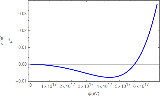
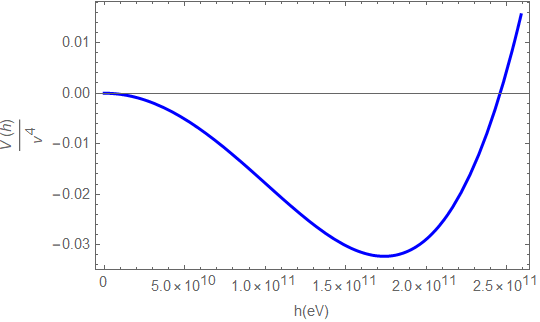
Figure 1: The axion potential of Eq. (10) for $\Lambda_{c}=m_{H}$ (left plot) and the Higgs potential (right plot) after the electroweak symmetry breaking.

As it can be seen, the axion potential is severely altered since a new minimum is generated, but still the new vacuum respects the misalignment mechanism which remains valid even with the dynamical effects of the extra Higgs-axion couplings after the electroweak symmetry breaking. More importantly, the Higgs vacuum is somewhat deeper, but energetically the two vacua are almost equivalent. Thus from a phenomenological point of view, scenario I is theoretically disfavored because it leads to an additional vacuum state in the Universe, which is equivalent to the Higgs vacuum. We would then have two competing vacua in the Universe, which is rather phenomenologically unacceptable and theoretically unmotivated. Apart from that, the axion field as a dark matter particle is basically eliminated since the new vacuum cannot decay to the Higgs vacuum and thus the new mass of the axion is of the order $\sim 0.47\,$GeV by using the values of the parameters with $\Lambda_{c}=m_{H}$. Thus, although this change in its mass is not a problem, the two competing vacua is an undesirable feature.

There is an additional reason which makes couplings of the form $m_{H}^{2}|H|^{2}\cos(\frac{\phi}{f_{a}})$ undesirable both phenomenologically and theoretically, apart from the reason we just described. The reason is that if we include the loop corrections effects at even one loop from the Higgs particle, the axion acquires huge corrections from the Higgs sector. We shall discuss this issue in the last section of this work. Let us mention that the theoretically unappealing features of couplings with $\Lambda_{c}\sim v$ were also discussed in Ref. [109].

II.2 Scenario II: Couplings of the Form $m_{\nu}^{2}|H|^{2}\cos(\frac{\phi}{f_{a}})$ and $m_{a}^{2}|H|^{2}\cos(\frac{\phi}{f_{a}})$

Now let us assume that the mass scale $\Lambda_{c}$ takes lower values than the case studied in the previous section. We shall consider two distinct scenarios, one in which case $\Lambda_{c}\sim\mathcal{O}(m_{\nu})$ and one case in which $\Lambda_{c}\sim\mathcal{O}(10^{-10}\times m_{a})$, where $m_{\nu}$ is the neutrino mass assumed to be of the order $m_{\nu}\sim 0.001\,$eV and the axion mass is $m_{a}\sim 10^{-10}\,$eV. We shall refer to this case as scenario II hereafter. Let us focus on the case $\Lambda_{c}\sim\mathcal{O}(m_{\nu})$, in which case the coupling $\lambda_{I}$ entering both the thermalization constraint and the branching ratio, $\lambda_{I}=\frac{\Lambda_{c}^{2}}{2f_{a}^{2}}$ is of the order $\lambda_{I}\sim\mathcal{O}(10^{-43})$, so the thermalization constraint $\lambda_{I}\leq 10^{-8}$ is satisfied and also the decay rate is of the order $\Gamma(h\to\phi\phi)\sim\mathcal{O}(10^{-75})$eV. Now let us study the axion effective potential in this case, so in Fig. 2 we plot the axionic effective potential given in Eq. (10), with $\Lambda_{c}\sim\mathcal{O}(m_{\nu})$

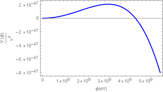
Figure 2: The axion potential of Eq. (10) for $\Lambda_{c}\sim\mathcal{O}(m_{\nu})$.

In this case we have quite intriguing phenomenology because the axion field develops a new energetically favorable minimum, compared to that in the origin, and also a barrier exists between the two vacua (see right plot). Thus the following phenomenological picture is implied: The axion will vacuum penetrate to the new vacuum via a first order phase transition possibly, and will acquire instantly a new vacuum expectation value. However, if we compare the axion potential with the Higgs potential in Fig. 1, it is apparent that the axion vacuum is not energetically favorable compared to the Higgs vacuum, thus the axion vacuum will decay to the Higgs vacuum. Thus the axion will return to the origin and the decay procedure will be perpetually repeated. It is expected that the axion phase transition can generate some imprint on the stochastic gravitational wave background corresponding to an era after the electroweak symmetry breaking, however we shall not go into details for this scenario, which will be covered elsewhere.

Now let us turn our focus on the case that $\Lambda_{c}=10^{-10}\times m_{a}$, with $m_{a}\sim 10^{-10}\,$eV. In this case the coupling $\lambda_{I}$ entering both the thermalization constraint and the decay rate of the Higgs to the axion field due to interactions $\sim h^{2}\phi^{2}$ ratio, $\lambda_{I}=\frac{\Lambda_{c}^{2}}{2f_{a}^{2}}$ is of the order $\lambda_{I}\sim\mathcal{O}(10^{-57})$, so in this case too the thermalization constraint $\lambda_{I}\leq 10^{-8}$ is satisfied and also the decay rate is of the order $\Gamma(h\to\phi\phi)\sim\mathcal{O}(10^{-103})$eV. Now let us proceed to the study of the axion effective potential in this case, so in Fig. 3 we plot the axionic effective potential given in Eq. (10), with $\Lambda_{c}\sim\mathcal{O}(10^{-10}\times m_{a})$.

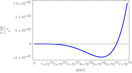
Figure 3: The axion potential of Eq. (10) for $\Lambda_{c}\sim\mathcal{O}(10^{-10}\times m_{a})$.

As we can see in this case, the axion develops a second minimum which is energetically favorable compared to the minimum at the origin, however no barrier exists between the two minima. In fact, we observed that as the mass scale evolves from values $\Lambda\sim m_{\nu}$ down to values $\Lambda_{c}\sim 10^{-15}\times m_{a}$, the barrier exists but it is significantly small, and is completely eliminated for values $\Lambda_{c}\sim 10^{-10}\times m_{a}$ or lower. The phenomenology in this case is quite different, because due to the existence of a second minimum with no barrier separating the two minima, the axion oscillations at the origin are interrupted. Thus after some considerable amount of time the axion will cease to oscillate and will roll down the new potential towards to the new minimum. Since the axion might be the sole component of dark matter, this rolling of the axion down its potential, will deform the background equation of state during this rolling era, from $w=1/3$ which corresponds to a radiation era, to a background EoS which is slightly smaller or larger than $w=1/3$, depending on whether the axion slowly rolls or fast rolls towards the new minimum. This background EoS deformation can have some imprint on the energy spectrum of the stochastic gravitational waves spectrum, as we evince shortly. However, when the axion reaches the new minimum, the new vacuum will decay to the Higgs vacuum, because the latter is energetically more favorable compared to the axionic vacuum. Thus the axion returns to the origin and the procedure is repeated perpetually. It is hard to estimate how many times this procedure occurs, thus we will assume that it occurs only once for simplicity. So for the analysis of the gravitational wave energy spectrum, we shall focus on the model with non-perturbative Higgs-axion couplings of the form $\sim\epsilon\Lambda_{c}^{2}|H|^{2}\cos(\frac{\phi}{f_{a}})$ with $\Lambda_{c}\sim 10^{-10}\times m_{a}$ and $m_{a}\sim 10^{-10}\,$eV. Before going to that, let us try to investigate how the axion oscillations are disturbed at the origin of its potential, with the potential being given by Eq. (10) for $\Lambda_{c}\sim\mathcal{O}(10^{-10}\times m_{a})$. Since the deformation of the axion potential occurs after the electroweak symmetry breaking, this means that the Hubble rate is described by the radiation domination era value $H(t)=\frac{2}{t}$. The evolution of the scalar field in terms of the cosmic time, is described by the Klein-Gordon equation in a Friedmann-Robertson-Walker background,

$$\ddot{\phi}+3H(t)\dot{\phi}+V^{\prime}(\phi)=0\,,$$ (14)

so we shall numerically solve the above equation for the scalar potential chosen as in Eq. (10) for $\Lambda_{c}\sim\mathcal{O}(10^{-10}\times m_{a})$ and for the rest of the parameters chosen as in all the previous cases. We assume that after the axion deformation of the potential, the axion oscillates near the origin and has non-zero velocity, and specifically that $\phi(0.00000001)=0.00001$eV and $\dot{\phi}(0.00000001)=0.0001$eV². Thus, in Fig. 4 we present the evolution of $\phi(t)$ and of $\dot{\phi}(t)$ as a function of the cosmic time.

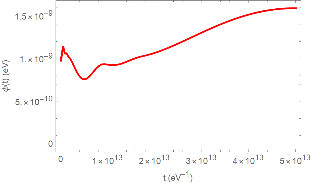
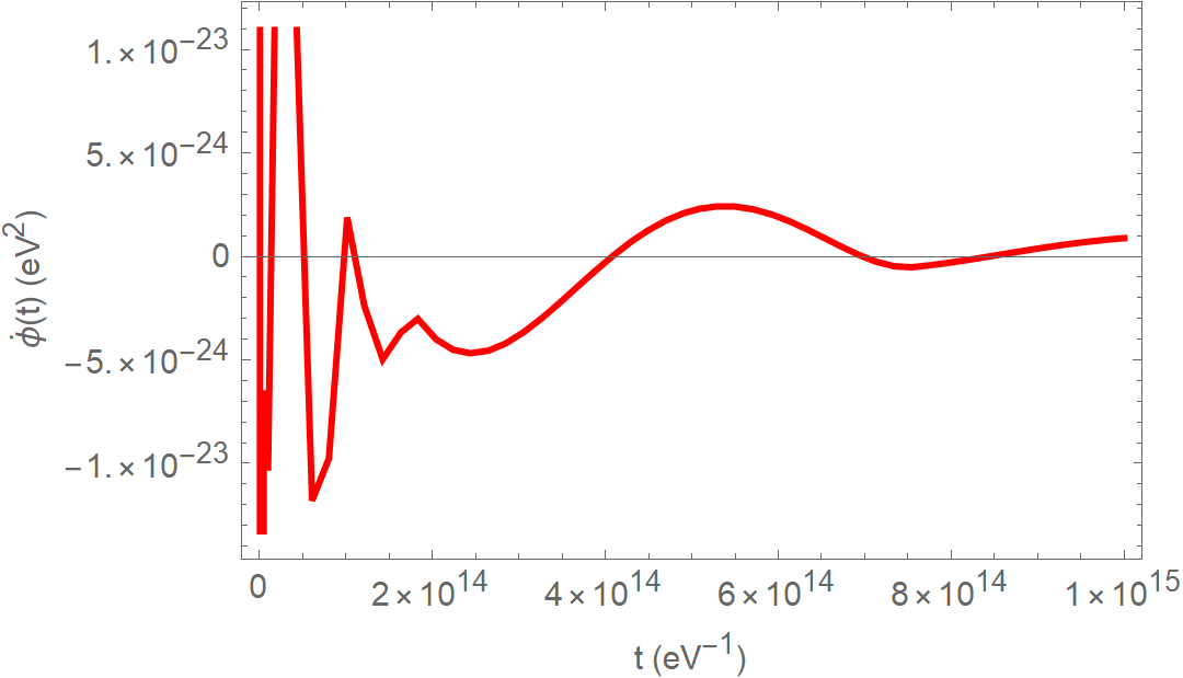
Figure 4: The evolution of the axion $\phi(t)$ versus time (left plot) at the origin of its effective potential, for the effective potential given in Eq. (10) and the evolution of $\dot{\phi}(t)$ versus time (right plot), for the initial conditions $\phi(0.00000001)=0.000000001$eV and $\dot{\phi}(0.00000001)=0.01$eV². This theory corresponds to non-perturbative Higgs-axion couplings of the form $\sim\epsilon\Lambda_{c}^{2}|H|^{2}\cos(\frac{\phi}{f_{a}})$ with $\Lambda_{c}\sim 10^{-10}\times m_{a}$ and $m_{a}\sim 10^{-10}\,$eV.

As it can be seen in Fig. 4, the axion is destabilized from its oscillations for $t\sim 10^{13}\,$eV${}^{-1}=10^{-2}$sec, which is quite fast, but it rolls with an incredibly small speed towards the new minimum. This result however depends on the initial conditions, so we shall assume that the evolution of the axion towards the minimum of its potential can be done in two ways, in a fast-roll way and in a slow-roll way and also that the whole procedure occurs just once. This feature can be supported numerically and it depends on the initial conditions of $\phi(t)$, if for example $\phi(0)\sim 0$, then the axion oscillates near the origin for quite long, even infinitely. This can be seen in Fig. 5 where it seems that the axion oscillates with a small amplitude for nearly $t\sim 10^{15}$sec, which amounts for 0.3 billion of years. This result is robust regardless the value of the speed of the axion, and it holds true even for relatively large values of $\dot{\phi}$.

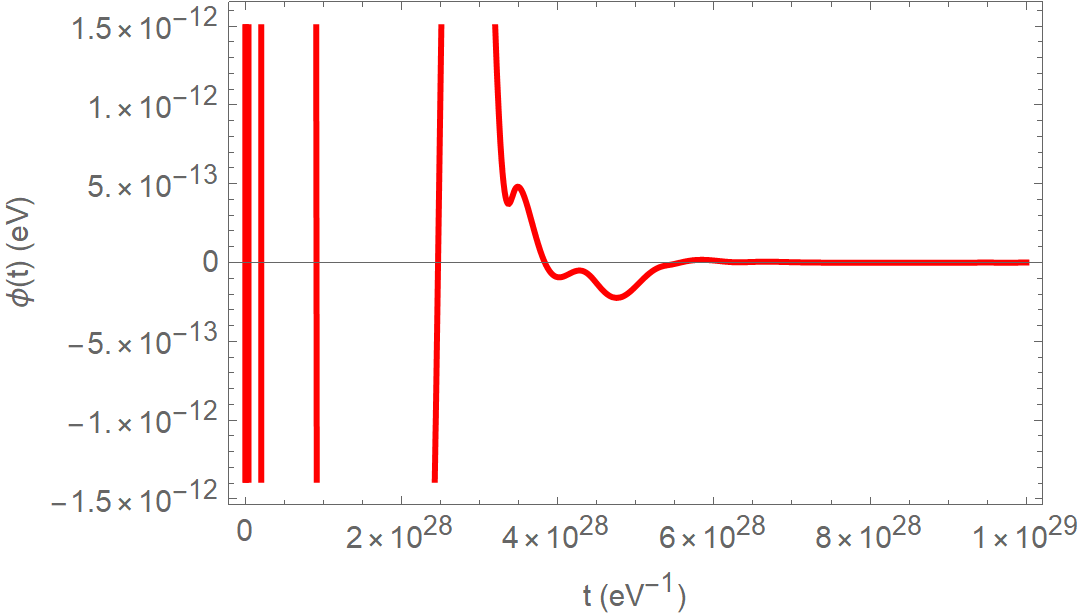
Figure 5: The evolution of the axion $\phi(t)$ versus time at the origin of its effective potential, for the effective potential given in Eq. (10), for the initial conditions $\phi(0.00000001)=0$eV and $\dot{\phi}(0.00000001)=0.01$eV². This behavior corresponds to non-perturbative Higgs-axion couplings of the form $\sim\epsilon\Lambda_{c}^{2}|H|^{2}\cos(\frac{\phi}{f_{a}})$ with $\Lambda_{c}\sim 10^{-10}\times m_{a}$ and $m_{a}\sim 10^{-10}\,$eV.

Thus, for models with non-perturbative Higgs-axion couplings of the form $\sim\epsilon\Lambda_{c}^{2}|H|^{2}\cos(\frac{\phi}{f_{a}})$ with $\Lambda_{c}\sim 10^{-10}\times m_{a}$ and $m_{a}\sim 10^{-10}\,$eV, we assume that after the axion rolls its potential once, and the new vacuum decays to the Higgs one, the axion returns to the origin with its vacuum energy converted to kinetic energy and it oscillates for a large amount of time before it will start rolling again. Hence, the deformation of the background EoS from its radiation domination value $w=1/3$ occurs only once. Now let us investigate the effect of this background EoS deformation on the energy spectrum of the stochastic gravitational waves. We assume two distinct models for the inflationary era, one with the standard red-tilted tensor spectral index, for example the $R^{2}$ model in the Jordan frame, or the corresponding model in the Einstein frame, well-known as Starobinsky model, in which $n_{\mathcal{T}}=-r/8$, and one model with a blue-tilted tensor spectral index, such as one of the Einstein-Gauss-Bonnet models developed in Refs. [111].

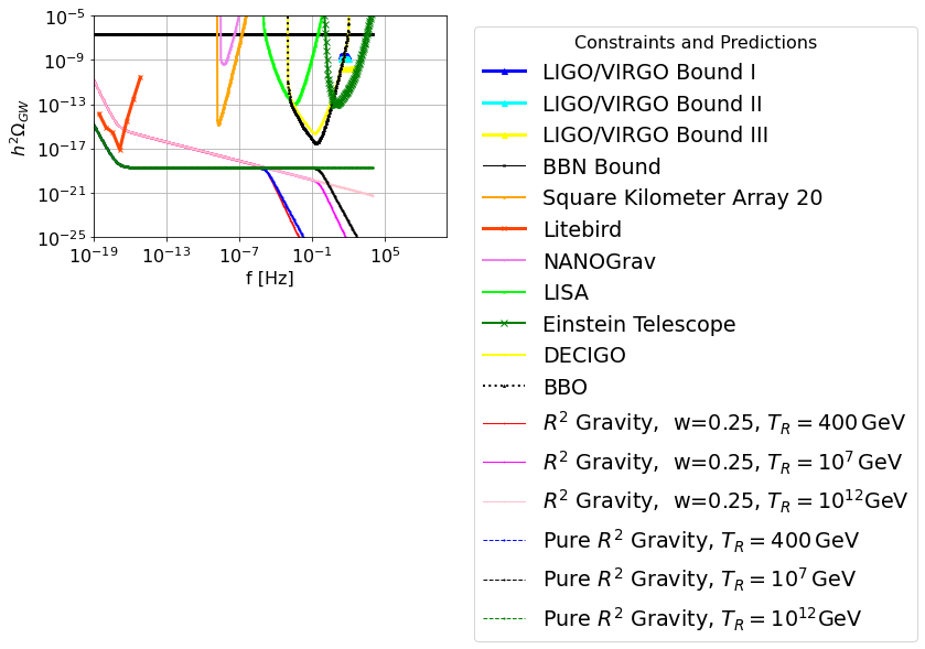
Figure 6: The $h^{2}$-scaled gravitational wave energy spectrum for an inflationary era described by $R^{2}$ theory with $n_{\mathcal{T}}=-r/8$ and $r=0.003$, with the deformed background EoS being and $w=0.25$ for frequencies probed by the Einstein telescope $k_{s}=6.5\times 10^{16}$Mpc^-1, and for three reheating temperatures $T_{R}=400\,$GeV, $T_{R}=10^{7}\,$GeV, and $T_{R}=10^{12}\,$GeV. This phenomenology is obtained for non-perturbative Higgs-axion couplings of the form $\sim\epsilon\Lambda_{c}^{2}|H|^{2}\cos(\frac{\phi}{f_{a}})$ with $\Lambda_{c}\sim 10^{-10}\times m_{a}$ and $m_{a}\sim 10^{-10}\,$eV.

For the analysis of the latter we will take that the tensor spectral index takes the value $n_{\mathcal{T}}=0.37$ and also the predicted tensor-to-scalar ratio is $r=0.003$, and the same applies for the Starobinsky model, with $n_{\mathcal{T}}=-r/8$ in this case however. Before proceeding, it is worth discussing in brief the inflationary theories we shall consider and the essential inflationary features of these. We start off with the $F(R)$ gravity theories which have the action,

$$\mathcal{S}=\frac{1}{2\kappa^{2}}\int\mathrm{d}^{4}x\sqrt{-g}F(R),$$ (15)

and the corresponding field equations for a flat Friedmann-Robertson-Walker metric are,

$$0= -\frac{F(R)}{2}+3\left(H^{2}+\dot{H}\right)F_{R}(R)-18\left(4H^{2}\dot{H}+H\ddot{H}\right)F_{RR}(R)\,,$$ (16)

$$0= \frac{F(R)}{2}-\left(\dot{H}+3H^{2}\right)F_{R}(R)+6\left(8H^{2}\dot{H}+4{\dot{H}}^{2}+6H\ddot{H}+\dddot{H}\right)F_{RR}(R)+36\left(4H\dot{H}+\ddot{H}\right)^{2}F_{RRR}\,,$$ (17)

with $F_{RR}=\frac{\mathrm{d}^{2}F}{\mathrm{d}R^{2}}$, and also $F_{RRR}=\frac{\mathrm{d}^{3}F}{\mathrm{d}R^{3}}$. Furthermore we assume that the slow-roll conditions are valid,

$$\ddot{H}\ll H\dot{H},\,\,\,\frac{\dot{H}}{H^{2}}\ll 1\,.$$ (18)

The inflationary indices, which capture the dynamics during the inflationary era, namely $\epsilon_{1}$ ,$\epsilon_{2}$, $\epsilon_{3}$, $\epsilon_{4}$, are [112, 113, 114],

$$\epsilon_{1}=-\frac{\dot{H}}{H^{2}},\quad\epsilon_{2}=0\,,\quad\epsilon_{3}=\frac{\dot{F}_{R}}{2HF_{R}}\,,\quad\epsilon_{4}=\frac{\ddot{F}_{R}}{H\dot{F}_{R}}\,,$$ (19)

and using these, we can express the spectral index of the scalar perturbations and also the tensor-to-scalar ratio in terms of these [113, 112],

$$n_{s}=1-\frac{4\epsilon_{1}-2\epsilon_{3}+2\epsilon_{4}}{1-\epsilon_{1}},\quad r=48\frac{\epsilon_{3}^{2}}{(1+\epsilon_{3})^{2}}\,.$$ (20)

Furthermore, by using the Raychaudhuri equation, we have,

$$\epsilon_{1}=-\epsilon_{3}(1-\epsilon_{4})\,,$$ (21)

therefore in view of the slow-roll conditions, we get approximately $\epsilon_{1}\simeq-\epsilon_{3}$, and in turn, the scalar spectral index takes the following form,

$$n_{s}\simeq 1-6\epsilon_{1}-2\epsilon_{4}\,,$$ (22)

and also the tensor-to-scalar ratio becomes,

$$r\simeq 48\epsilon_{1}^{2}\,.$$ (23)

Regarding the slow-roll index $\epsilon_{4}$, defined as $\epsilon_{4}=\frac{\ddot{F}_{R}}{H\dot{F}_{R}}$ we get,

$$\epsilon_{4}=\frac{\ddot{F}_{R}}{H\dot{F}_{R}}=\frac{\frac{d}{dt}\left(F_{RR}\dot{R}\right)}{HF_{RR}\dot{R}}=\frac{F_{RRR}\dot{R}^{2}+F_{RR}\frac{d(\dot{R})}{dt}}{HF_{RR}\dot{R}}\,,$$ (24)

and also by using,

$$\dot{R}=24\dot{H}H+6\ddot{H}\simeq 24H\dot{H}=-24H^{3}\epsilon_{1}\,,$$ (25)

and in conjunction with Eq. (24) we get,

$$\epsilon_{4}\simeq-\frac{24F_{RRR}H^{2}}{F_{RR}}\epsilon_{1}-3\epsilon_{1}+\frac{\dot{\epsilon}_{1}}{H\epsilon_{1}}\,.$$ (26)

Also by using,

$$\dot{\epsilon}_{1}=-\frac{\ddot{H}H^{2}-2\dot{H}^{2}H}{H^{4}}=-\frac{\ddot{H}}{H^{2}}+\frac{2\dot{H}^{2}}{H^{3}}\simeq 2H\epsilon_{1}^{2}\,,$$ (27)

the slow-roll index $\epsilon_{4}$ finally becomes,

$$\epsilon_{4}\simeq-\frac{24F_{RRR}H^{2}}{F_{RR}}\epsilon_{1}-\epsilon_{1}\,.$$ (28)

Accordingly the tensor spectral index can be evaluated using [112, 113, 115],

$$n_{\mathcal{T}}\simeq-2(\epsilon_{1}+\epsilon_{3})\,,$$ (29)

hence by using Eq. (28) we get,

$$n_{\mathcal{T}}\simeq-2\frac{\epsilon_{1}^{2}}{1+\epsilon_{1}}\simeq-2\epsilon_{1}^{2}\,.$$ (30)

Regarding the $R^{2}$ model, we get,

$$n_{\mathcal{T}}\simeq-\frac{1}{2N^{2}}\,,$$ (31)

therefore for $N=60$ we have $n_{\mathcal{T}}=-0.000138889$, $n_{s}\simeq 0.963$ and $r\simeq 0.0033$, which we shall use for the plots of the gravitational waves energy spectrum.

Regarding the Einstein-Gauss-Bonnet theories, the gravitational action is,

$$\centering S=\int{d^{4}x\sqrt{-g}\left(\frac{R}{2\kappa^{2}}-\frac{1}{2}\partial_{\mu}\phi\partial^{\mu}\phi-V(\phi)-\frac{1}{2}\xi(\phi)\mathcal{G}\right)}\,,\@add@centering$$ (32)

where $\mathcal{G}$ denotes the Gauss-Bonnet invariant which is $\mathcal{G}=R^{2}-4R_{\alpha\beta}R^{\alpha\beta}+R_{\alpha\beta\gamma\delta}R^{\alpha\beta\gamma\delta}$ with $R_{\alpha\beta}$ and $R_{\alpha\beta\gamma\delta}$ are the Ricci and Riemann tensors respectively. The propagation speed of the gravitational tensor perturbations is required to be equal to unity in Einstein-Gauss-Bonnet theories, hence by using this, the slow-roll indices for the Einstein-Gauss-Bonnet theory become [111],

$$\centering\epsilon_{1}\simeq\frac{\kappa^{2}}{2}\left(\frac{\xi^{\prime}}{\xi^{\prime\prime}}\right)^{2}\,,\@add@centering$$ (33)

$$\centering\epsilon_{2}\simeq 1-\epsilon_{1}-\frac{\xi^{\prime}\xi^{\prime\prime\prime}}{\xi^{\prime\prime 2}}\,,\@add@centering$$ (34)

$$\centering\epsilon_{3}=0\,,\@add@centering$$ (35)

$$\centering\epsilon_{4}\simeq\frac{\xi^{\prime}}{2\xi^{\prime\prime}}\frac{\mathcal{E}^{\prime}}{\mathcal{E}}\,,\@add@centering$$ (36)

$$\centering\epsilon_{5}\simeq-\frac{\epsilon_{1}}{\lambda}\,,\@add@centering$$ (37)

$$\centering\epsilon_{6}\simeq\epsilon_{5}(1-\epsilon_{1})\,,\@add@centering$$ (38)

with $\mathcal{E}=\mathcal{E}(\phi)$ and in addition $\lambda=\lambda(\phi)$ are,

$$\mathcal{E}(\phi)=\frac{1}{\kappa^{2}}\left(1+72\frac{\epsilon_{1}^{2}}{\lambda^{2}}\right),\,\,\,\lambda(\phi)=\frac{3}{4\xi^{\prime\prime}\kappa^{2}V}\,.$$ (39)

Thus, the inflationary observational indices can be obtained, which are,

$$\centering n_{\mathcal{S}}=1-4\epsilon_{1}-2\epsilon_{2}-2\epsilon_{4}\,,\@add@centering$$ (40)

$$n_{\mathcal{T}}=-2\left(\epsilon_{1}+\epsilon_{6}\right)\,,$$ (41)

$$r=16\left|\left(\frac{\kappa^{2}Q_{e}}{4H}-\epsilon_{1}\right)\frac{2c_{A}^{3}}{2+\kappa^{2}Q_{b}}\right|\,,$$ (42)

where $c_{A}$ stands for the sound speed of the scalar perturbations, which has the following form,

$$\centering c_{A}^{2}=1+\frac{Q_{a}Q_{e}}{3Q_{a}^{2}+\dot{\phi}^{2}(\frac{2}{\kappa^{2}}+Q_{b})}\,,\@add@centering$$ (43)

with,

$$Q_{a}=-4\dot{\xi}H^{2},\,\,\,Q_{b}=-8\dot{\xi}H,\,\,\,Q_{t}=F+\frac{Q_{b}}{2},$$ (44)

$$Q_{c}=0,\,\,\,Q_{e}=-16\dot{\xi}\dot{H}\,.$$

Thus, the tensor-to-scalar ratio and the tensor spectral index become,

$$r\simeq 16\epsilon_{1}\,,$$ (45)

$$n_{\mathcal{T}}\simeq-2\epsilon_{1}\left(1-\frac{1}{\lambda}+\frac{\epsilon_{1}}{\lambda}\right)\,.$$ (46)

A viable Einstein-Gauss-Bonnet model has the following Gauss-Bonnet coupling function [111],

$$\xi(\phi)=\beta\exp\left(\left(\frac{\phi}{M}\right)^{2}\right)\,,$$ (47)

where $\beta$ is a dimensionless parameter and also $M$ has mass dimensions $[m]^{1}$. The potential for this theory is derived to be,

$$\centering V(\phi)=\frac{3}{3\gamma\kappa^{4}+4\beta\kappa^{4}e^{\frac{\phi^{2}}{M^{2}}}}\,,\@add@centering$$ (48)

where $\gamma$ a dimensionless an integration constant. Accordingly, the slow-roll indices are,

$$\centering\epsilon_{1}\simeq\frac{\kappa^{2}M^{4}\phi^{2}}{2\left(M^{2}+2\phi^{2}\right)^{2}}\,,\@add@centering$$ (49)

$$\centering\epsilon_{2}\simeq\frac{M^{4}\left(2-\kappa^{2}\phi^{2}\right)-4M^{2}\phi^{2}}{2\left(M^{2}+2\phi^{2}\right)^{2}}\,,\@add@centering$$ (50)

$$\centering\epsilon_{3}=0\,,\@add@centering$$ (51)

$$\centering\epsilon_{5}\simeq-\frac{4\beta\phi^{2}e^{\frac{\phi^{2}}{M^{2}}}}{\left(M^{2}+2\phi^{2}\right)\left(3\gamma+4\beta e^{\frac{\phi^{2}}{M^{2}}}\right)}\,,\@add@centering$$ (52)

$$\centering\epsilon_{6}\simeq-\frac{2\beta\phi^{2}e^{\frac{\phi^{2}}{M^{2}}}\left(M^{4}\left(2-\kappa^{2}\phi^{2}\right)+8M^{2}\phi^{2}+8\phi^{4}\right)}{\left(M^{2}+2\phi^{2}\right)^{3}\left(3\gamma+4\beta e^{\frac{\phi^{2}}{M^{2}}}\right)}\,,\@add@centering$$ (53)

and in addition, the scalar spectral index, the tensor spectral index and the corresponding tensor-to-scalar ratio are,

$$n_{\mathcal{S}}\simeq-1-\frac{\kappa^{2}M^{4}\phi^{2}}{\left(M^{2}+2\phi^{2}\right)^{2}}+\frac{4\phi^{2}\left(3M^{2}+2\phi^{2}\right)}{\left(M^{2}+2\phi^{2}\right)^{2}}$$ (54)

$$+\frac{4608\beta^{2}\phi^{6}e^{\frac{2\phi^{2}}{M^{2}}}\left(6\gamma\phi^{2}+16\beta e^{\frac{\phi^{2}}{M^{2}}}\left(M^{2}+\phi^{2}\right)+9\gamma M^{2}\right)}{\left(M^{2}+2\phi^{2}\right)^{4}\left(3\gamma+4\beta e^{\frac{\phi^{2}}{M^{2}}}\right)^{3}}\,,$$

and also

$$n_{\mathcal{T}}\simeq\frac{\phi^{2}\left(-4\beta e^{\frac{\phi^{2}}{M^{2}}}\left(M^{4}\left(3\kappa^{2}\phi^{2}-2\right)+\kappa^{2}M^{6}-8M^{2}\phi^{2}-8\phi^{4}\right)-3\gamma\kappa^{2}M^{4}\left(M^{2}+2\phi^{2}\right)\right)}{\left(M^{2}+2\phi^{2}\right)^{3}\left(3\gamma+4\beta e^{\frac{\phi^{2}}{M^{2}}}\right)}\,,$$ (55)

$$r\simeq\frac{8\kappa^{2}M^{4}\phi^{2}}{\left(M^{2}+2\phi^{2}\right)^{2}}\,.$$ (56)

For the analysis and plots of the gravitational wave energy spectrum we shall use the following values for the free parameters $\mu=[22.0914,22.09147]$, $\beta=-1.5$, $\gamma=2$, for approximately $N=60$ $e$-foldings, and for these we have $n_{\mathcal{T}}=[0.378,0.379]$ and $r\sim 0.003$, which are what we shall use for the gravitational wave analysis and plots. We will also assume three distinct cases for the reheating temperature, the following, $T_{R}=400\,$GeV, thus a low-reheating temperature scenario, $T_{R}=10^{7}\,$GeV, thus an intermediate-reheating temperature scenario, and finally a high reheating temperature scenario with $T_{R}=10^{12}\,$GeV. We shall also assume that the axion rolling towards the new minimum occurs once during the radiation domination era, and at frequencies probed by the Einstein telescope, thus for wavenumbers of the order $k_{s}=6.5\times 10^{16}$Mpc^-1. Since there are two ways for the axion to roll towards the new minimum of its potential, one slow-roll and one fast-roll, the deformation of the background EoS will be assumed to be either $w=0.25$, thus smaller than $w=1/3$, or $w=0.35$, which is larger than the radiation domination epoch value.

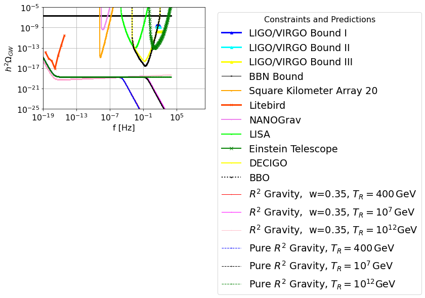
Figure 7: The $h^{2}$-scaled gravitational wave energy spectrum for an inflationary era described by $R^{2}$ theory with $n_{\mathcal{T}}=-r/8$ and $r=0.003$, with the deformed background EoS being and $w=0.35$ for frequencies probed by the Einstein telescope $k_{s}=6.5\times 10^{16}$Mpc^-1, and for three reheating temperatures $T_{R}=400\,$GeV, $T_{R}=10^{7}\,$GeV, and $T_{R}=10^{12}\,$GeV. This phenomenological behavior is obtained for non-perturbative Higgs-axion couplings of the form $\sim\epsilon\Lambda_{c}^{2}|H|^{2}\cos(\frac{\phi}{f_{a}})$ with $\Lambda_{c}\sim 10^{-10}\times m_{a}$ and $m_{a}\sim 10^{-10}\,$eV.

The effect of a background EoS deformation during the reheating era on the energy spectrum of the gravitational waves is quantified by a multiplication factor, $\sim\left(\frac{k}{k_{s}}\right)^{r_{c}}$, where $r_{c}=-2\left(\frac{1-3w}{1+3w}\right)$ [116], where $k_{s}$ is the wavenumber at which the deformation of the background EoS occurs.

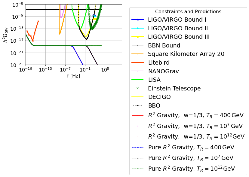
Figure 8: The $h^{2}$-scaled gravitational wave energy spectrum for an inflationary era described by $R^{2}$ theory with $n_{\mathcal{T}}=-r/8$ and $r=0.003$, with the background EoS being $w=1/3$ and for three reheating temperatures $T_{R}=400\,$GeV, $T_{R}=10^{7}\,$GeV, and $T_{R}=10^{12}\,$GeV. This phenomenology is obtained for models with non-perturbative Higgs-axion couplings of the form $\sim\epsilon\Lambda_{c}^{2}|H|^{2}\cos(\frac{\phi}{f_{a}})$ with $\Lambda_{c}\sim 10^{-10}\times m_{a}$ and $m_{a}\sim 10^{-10}\,$eV.

This will multiply the $h^{2}$-scaled energy spectrum of the primordial gravitational waves, thus including the effect of the deformation of the background EoS, the present day $h^{2}$-scaled energy spectrum of the primordial gravitational waves takes the form,

$$\Omega_{\rm gw}(f)=S_{k}(f)\times\frac{k^{2}}{12H_{0}^{2}}r\mathcal{P}_{\zeta}(k_{ref})\left(\frac{k}{k_{ref}}\right)^{n_{\mathcal{T}}}\left(\frac{\Omega_{m}}{\Omega_{\Lambda}}\right)^{2}\left(\frac{g_{*}(T_{\rm in})}{g_{*0}}\right)\left(\frac{g_{*s0}}{g_{*s}(T_{\rm in})}\right)^{4/3}\left(\overline{\frac{3j_{1}(k\tau_{0})}{k\tau_{0}}}\right)^{2}T_{1}^{2}\left(x_{\rm eq}\right)T_{2}^{2}\left(x_{R}\right)\,,$$ (57)

with $S_{k}(f)$,

$$S_{k}(f)=\left(\frac{k}{k_{s}}\right)^{r_{s}}\,,$$ (58)

where $k_{ref}$ is the CMB pivot scale $k_{ref}=0.002$ Mpc^-1, and $n_{\mathcal{T}}$ and $r$ stand for the tensor spectral index of the primordial tensor perturbations and the tensor-to-scalar ratio. Also $T_{\rm in}$ denotes the temperature at the horizon reentry,

$$T_{\rm in}\simeq 5.8\times 10^{6}~{}{\rm GeV}\left(\frac{g_{*s}(T_{\rm in})}{106.75}\right)^{-1/6}\left(\frac{k}{10^{14}~{}{\rm Mpc^{-1}}}\right)\,,$$ (59)

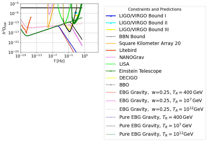
Figure 9: The $h^{2}$-scaled gravitational wave energy spectrum for an inflationary era described by an Einstein-Gauss-Bonnet theory with $n_{\mathcal{T}}=0.37$ and $r=0.003$, with the deformed background EoS being and $w=0.25$ for frequencies probed by the Einstein telescope $k_{s}=6.5\times 10^{16}$Mpc^-1, and for three reheating temperatures $T_{R}=400\,$GeV, $T_{R}=10^{7}\,$GeV, and $T_{R}=10^{12}\,$GeV. This gravitational wave phenomenology is obtained for non-perturbative Higgs-axion couplings of the form $\sim\epsilon\Lambda_{c}^{2}|H|^{2}\cos(\frac{\phi}{f_{a}})$ with $\Lambda_{c}\sim 10^{-10}\times m_{a}$ and $m_{a}\sim 10^{-10}\,$eV.

and also the transfer function $T_{1}(x_{\rm eq})$ stands for,

$$T_{1}^{2}(x_{\rm eq})=\left[1+1.57x_{\rm eq}+3.42x_{\rm eq}^{2}\right],$$ (60)

with $x_{\rm eq}=k/k_{\rm eq}$ and $k_{\rm eq}\equiv a(t_{\rm eq})H(t_{\rm eq})=7.1\times 10^{-2}\Omega_{m}h^{2}$ Mpc^-1, while the transfer function $T_{2}(x_{R})$ is equal to,

$$T_{2}^{2}\left(x_{R}\right)=\left(1-0.22x^{1.5}+0.65x^{2}\right)^{-1}\,,$$ (61)

with $x_{R}=\frac{k}{k_{R}}$, and the wavenumber at reheating temperature is,

$$k_{R}\simeq 1.7\times 10^{13}~{}{\rm Mpc^{-1}}\left(\frac{g_{*s}(T_{R})}{106.75}\right)^{1/6}\left(\frac{T_{R}}{10^{6}~{}{\rm GeV}}\right)\,,$$ (62)

where $T_{R}$ denotes the reheating temperature. Finally, $g_{*}(T_{\mathrm{in}}(k))$ stands for [117],

$$g_{*}(T_{\mathrm{in}}(k))=g_{*0}\left(\frac{A+\tanh\left[-2.5\log_{10}\left(\frac{k/2\pi}{2.5\times 10^{-12}\mathrm{Hz}}\right)\right]}{A+1}\right)\left(\frac{B+\tanh\left[-2\log_{10}\left(\frac{k/2\pi}{6\times 10^{-19}\mathrm{Hz}}\right)\right]}{B+1}\right)\,,$$ (63)

where $A$ and $B$ are equal to,

$$A=\frac{-1-10.75/g_{*0}}{-1+10.75g_{*0}}\,,$$ (64)

$$B=\frac{-1-g_{max}/10.75}{-1+g_{max}/10.75}\,,$$ (65)

with $g_{max}=106.75$ and $g_{*0}=3.36$. Furthermore $g_{*0}(T_{\mathrm{in}}(k))$ can be calculated by using Eqs. (63), (64) and (65), by replacing $g_{*0}=3.36$ with $g_{*s}=3.91$. Now let us proceed to the analysis of the $h^{2}$-scaled energy spectrum of the primordial gravitational waves including the effects of the deformation of the background EoS. In Figs. 6 and 7 we plot the $h^{2}$-scaled gravitational wave energy spectrum for an inflationary era described by the Starobinsky model with $n_{\mathcal{T}}=-r/8$ and $r=0.003$, with a deformed background EoS $w=0.25$ (Fig. 6) and $w=0.35$ (Fig. 7) occurring for frequencies probed by the Einstein telescope $k_{s}=6.5\times 10^{16}$Mpc^-1, for three reheating temperatures $T_{R}=400\,$GeV, $T_{R}=10^{7}\,$GeV, and $T_{R}=10^{12}\,$GeV, for both the pure and broken power-law cases. In addition, in Fig. 8 we plot the energy spectrum of the primordial gravitational waves for $w=1/3$ for ordinary $R^{2}$ gravity without the broken power-law for frequencies above the Einstein Telescope, and with the broken power-law modifications. Also in Figs. 9 and 10 we plot the $h^{2}$-scaled gravitational wave energy spectrum for an inflationary era described by an Einstein-Gauss-Bonnet theory with $n_{\mathcal{T}}=0.37$ and $r=0.003$, with the deformed background EoS being $w=0.25$ (Fig. 9) and $w=0.35$ (Fig. 10) occurring in this case too for frequencies probed by the Einstein telescope $k_{s}=6.5\times 10^{16}$Mpc^-1, and again for three reheating temperatures $T_{R}=400\,$GeV, $T_{R}=10^{7}\,$GeV, and $T_{R}=10^{12}\,$GeV, including the pure Einstein-Gauss-Bonnet case without the broken power-law scenarios. In all the plots we included the sensitivity curves from the most prominent future gravitational wave experiments, and also the constraints from the Big Bang Nucleosynthesis and the constraints from LIGO-Virgo.

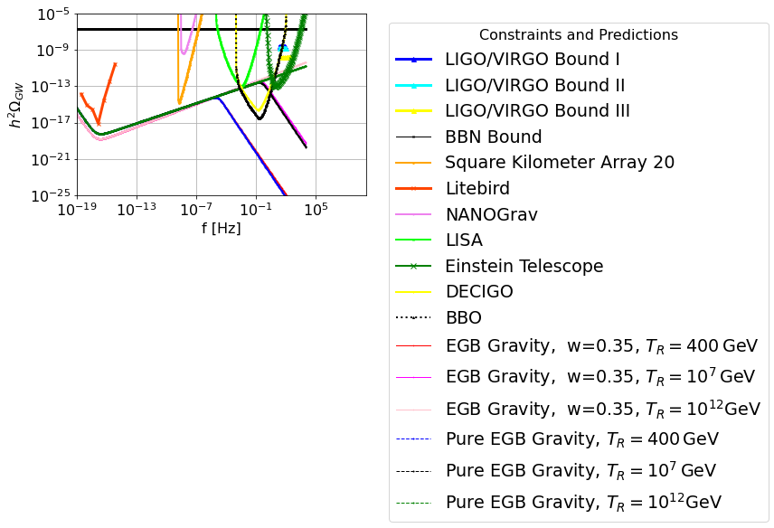
Figure 10: The $h^{2}$-scaled gravitational wave energy spectrum for an inflationary era described by an Einstein-Gauss-Bonnet theory with $n_{\mathcal{T}}=0.37$ and $r=0.003$, with the deformed background EoS being and $w=0.35$ for frequencies probed by the Einstein telescope $k_{s}=6.5\times 10^{16}$Mpc^-1, and for three reheating temperatures $T_{R}=400\,$GeV, $T_{R}=10^{7}\,$GeV, and $T_{R}=10^{12}\,$GeV. This phenomenology for gravitational waves is obtained for non-perturbative Higgs-axion couplings of the form $\sim\epsilon\Lambda_{c}^{2}|H|^{2}\cos(\frac{\phi}{f_{a}})$ with $\Lambda_{c}\sim 10^{-10}\times m_{a}$ and $m_{a}\sim 10^{-10}\,$eV.

Let us analyze the resulting picture at this point and we consider the $R^{2}$ case first. As it can be seen in Figs. 7 and 8, the energy spectrum remains undetectable for ordinary $R^{2}$ gravity without the broken power-law above the Einstein Telescope frequencies, however for a broken power-law above the Einstein Telescope frequencies with a deformed background EoS equal to $w=0.25$, the energy spectrum of the primordial gravitational waves is detectable by the Litebird experiment as can be seen in Fig. 6. However, for the case of $R^{2}$ gravity with a broken power-law above the Einstein Telescope frequencies, with a deformed background EoS equal to $w=0.35$, the energy spectrum of the primordial gravitational waves is undetectable by all the future experiments and in fact resembles the pure $R^{2}$ scenario. Thus for $w<1/3$ the differences between the pure and deformed $R^{2}$ scenarios are more pronounced. However for $w=1/3$ the broken power-law $R^{2}$ results and the pure $R^{2}$ ones are indistinguishable, as it can be seen in Fig. 8. Regarding the Einstein-Gauss-Bonnet theories with $n_{\mathcal{T}}=0.37$ and $r=0.003$, the signal for a broken power-law above the Einstein Telescope frequencies, with a deformed background EoS equal to $w=0.25$, the signal is detectable only by the Litebird, and the SKA for a small reheating temperature, by Litebird, LISA, BBO and DECIGO for intermediate reheating temperatures, and by Litebird, LISA, BBO, DECIGO and the Einstein Telescope for a large reheating temperature, as it can be seen in Fig. 9. Finally, for Einstein-Gauss-Bonnet theories with $n_{\mathcal{T}}=0.37$ and $r=0.003$, the signal for a broken power-law above the Einstein Telescope frequencies, with a deformed background EoS equal to $w=0.35$, the signal is undetectable for a small reheating temperature, is detectable by BBO and DECIGO for intermediate reheating temperatures, and detectable by BBO, DECIGO and the Einstein Telescope for a large reheating temperature, as it can be seen in Fig. 10. Also, as in the $R^{2}$ case, the differences between pure Einstein-Gauss-Bonnet theory and broken power-law Einstein-Gauss-Bonnet theory is more pronounced when $w<1/3$. Now the resulting picture is quite illuminating since it offers a unique pattern for future stochastic gravitational wave detection. The important information offered is the pattern of detection by Litebird and the rest of the future experiments. The predictions provide information about the tensor spectral index, if it is positive or negative, and also provides information about the reheating temperature, if it is high, intermediate or small. Furthermore what is mentionable is the detection from Litebird in both the red-tilted and blue-tilted inflation, especially for the former. This information can be valuable for future stochastic gravitational wave detections, since our analysis provides specific patterns of detections. Thus a synergy between all the future gravitational waves experiments can yield important insights towards finding the correct underlying theory that produces the future detected pattern of stochastic gravitational waves.

III Corrections to the Misalignment Axion Potential due to Higgs Loops

Now let us consider another important feature brought in the theory of axion-Higgs interactions by couplings of the form $\sim\epsilon\L_{c}^{2}|H|^{2}\cos(\frac{\phi}{f_{a}})$. Now with these couplings present, if one takes into account one-loop Higgs corrections, the following quantum correction terms arise in the theory [109],

$$\epsilon\Lambda_{c}^{4}\cos(\frac{\phi}{f_{a}})\,,$$ (66)

at leading order in the dimensionless parameter $\epsilon$ which is considered to be smaller than unity. So effectively if one takes into account the misalignment approximation in the regime $\phi\ll f_{a}$, the above quantum corrections result in the following terms that must be added to the effective potential of the axion, at leading order in $\phi$,

$$V^{quantum}(\phi)=\epsilon\Lambda_{c}^{4}-\frac{\epsilon\Lambda_{c}^{4}}{2f_{a}^{2}}\phi^{2}+\frac{\epsilon\Lambda_{c}^{4}}{24f_{a}^{4}}\phi^{4}\,,$$ (67)

so the effective potential of the axion becomes,

$$V(\phi)=\frac{\Lambda_{c}^{2}v^{2}\phi^{4}\epsilon}{48f_{a}^{4}}-\frac{\Lambda_{c}^{2}v^{2}\phi^{2}\epsilon}{4f_{a}^{2}}+m_{a}^{2}\left(1-\cos\left(\frac{x}{f_{a}}\right)\right)+\frac{gv^{2}\phi^{6}}{2M^{4}}-\frac{\lambda v^{2}\phi^{4}}{2M^{2}}$$ (68)

$$-\frac{\Lambda_{c}^{2}v^{2}\phi^{6}\epsilon}{1440f_{a}^{6}}+\frac{\Lambda_{c}^{4}\phi^{4}\epsilon}{24f_{a}^{4}}-\frac{\Lambda_{c}^{4}\phi^{2}\epsilon}{2f_{a}^{2}}+\frac{m_{eff}^{4}\left(\log\left(\frac{m_{eff}^{2}}{\mu^{2}}\right)-\frac{3}{2}\right)}{64\pi^{2}}+\Lambda_{c}^{4}\epsilon\,,$$

where $m_{eff}^{2}$ in this case reads,

$$m_{eff}^{2}=\frac{\Lambda_{c}^{2}v^{2}\phi^{4}\epsilon}{48f_{a}^{6}}-\frac{\Lambda_{c}^{2}v^{2}\phi^{2}\epsilon}{4f_{a}^{4}}+\frac{\Lambda_{c}^{4}\phi^{2}\epsilon}{2f_{a}^{4}}+\frac{\Lambda_{c}^{2}v^{2}\epsilon}{2f_{a}^{2}}-\frac{\Lambda_{c}^{4}\epsilon}{f_{a}^{2}}+\frac{\phi^{4}\left(15gv^{2}\right)}{M^{4}}-\frac{\phi^{2}\left(6\lambda v^{2}\right)}{M^{2}}+m_{a}^{2}\,.$$ (69)

A noticeable feature brought by the quantum corrections is the presence of a constant vacuum energy term $\sim\epsilon\Lambda_{c}^{4}$. Now regarding the phenomenology, we shall assume that $\epsilon\sim\mathcal{O}(0.1)$, so we consider all the scenarios we discussed in the previous sections. The resulting phenomenological picture is quite similar to the case where the quantum corrections were not included. Particularly, for an effective theory of $M\sim 20\,$TeV, the case with $\Lambda_{c}\sim 125\,$GeV leads to a new vacuum state for the axion which is energetically equivalent with the Higgs vacuum, so this scenario is rather phenomenologically unviable, plus a large vacuum energy of the order $\sim\epsilon\Lambda_{c}^{4}$ is induced. Now the case with $\Lambda_{c}\sim 10^{-3}\,$eV is quite interesting, since a small constant vacuum energy term is induced and also the phenomenological picture is the same with the case that the quantum corrections were not included, except for the fact that the barrier between the new and old axion vacua does not exist. Thus the axion is free to roll down to its new minimum, a scenario which was described in detail in the previous sections. The same applies for the case $\Lambda_{c}\sim 10^{-20}\,$eV, in which case a small constant vacuum energy term is induced too.

Concluding Remarks and Discussion

In this work we considered some of the most possible Higgs-axion couplings and we investigated the phenomenological implications of such couplings. Specifically, we assumed that the axion is coupled to a weakly coupled effective theory with the energy scale $M$ of the effective theory being of the order of $M\sim\mathcal{O}(20)\,$TeV, and the Wilson coefficients of the order $\mathcal{O}(10^{-35})\,$TeV, in the presence of non-perturbative couplings of the form $\sim\epsilon\Lambda_{c}^{2}|H|^{2}\cos(\frac{\phi}{f_{a}})$ with $\Lambda_{c}$ being an arbitrary mass scale. Due to the fact that we consider the misalignment axion, during and in the post-inflationary era, the axion satisfies $\phi\ll f_{a}$, thus the non-perturbative coupling can be expanded in perturbation series in terms of $\phi/f_{a}$ and eventually we may have a leading order approximation for the axion effective potential after the electroweak symmetry breaking. We derive the axion effective potential at one loop and we investigate the phenomenological implications of the couplings $\sim\epsilon\Lambda_{c}^{2}|H|^{2}\cos(\frac{\phi}{f_{a}})$ combined with the higher order non-renormalizable operators. As we demonstrated, depending on the value of the mass scale $\Lambda_{c}$, the implied changes in the misaligned axion effective potential are drastic. For all the cases, we took into account the constraints imposed by the LHC experiment on the branching ratio of the Higgs to an invisible electroweak singlet scalar hidden sector, and also the thermalization constraints, since we need the axion to be a non-thermal relic. The case $\Lambda_{c}\sim\mathcal{O}(m_{H})\,$, with $m_{H}$ being the Higgs mass, resulted to undesirable features in the effective potential since the axion potential develops a second minimum which is energetically equivalent to the Higgs vacuum, thus we have two competing vacua in the theory. The case $\Lambda_{c}\sim\mathcal{O}(m_{\nu})$, where $m_{\nu}$ is the neutrino mass, resulted to a theory in which the axion develops a new minimum which is energetically much less deep compared to the Higgs minimum and the minimum of the axion potential at the origin is separated by a barrier from the new axion minimum. Thus a post-electroweak era first order phase transition might occur in the axion sector, which might induce some detectable features in the stochastic gravitational wave energy spectrum, but we did not proceed in depth this phenomenological possibility. Finally, the case $\Lambda_{c}\sim\mathcal{O}(10^{-20})\,$eV resulted to a phenomenologically interesting situation. The axion develops a new minimum in its effective potential which is energetically more favorable than the minimum at the origin and with no barrier existing between the two vacua. As the axion now is destabilized, the axion oscillations at the origin are disturbed and the axion is free to roll down to its potential towards the new minimum of this potential. This can be done either in a slow-roll or fast-roll way. Since this roll of the axion occurs during the radiation domination era, the background EoS of the Universe might be affected by this rolling of the axion, because the axion composes the dark matter and this rolling affects somewhat the total EoS making it slightly larger (fast-roll) or smaller (slow-roll) than the radiation domination value $w=1/3$. If we assume that this rolling of the axion occurs during the radiation domination for frequencies probed by the Einstein Telescope, the deformation of the background EoS might have detectable effects on the energy spectrum of the primordial gravitational waves, resulting to a broken power-law multiplication factor in the total energy spectrum of the primordial gravitational waves. We examined the energy spectrum of the primordial gravitational waves for two inflationary scenarios, one with red-tilted tensor spectral index and one with blue-tilted tensor spectral index for two total background EoS parameters, $w=0.25$ and $w=0.35$. As we showed in Fig. 8, the energy spectrum of the primordial gravitational waves remains undetectable for the red-tilted inflationary era, without the broken power-law above the Einstein Telescope frequencies, however for a broken power-law scenario above the Einstein Telescope frequencies with a deformed background EoS equal to $w=0.25$, the energy spectrum of the primordial gravitational waves can be detectable by the Litebird experiment as can be seen in Fig. 6. However, for the a deformed background EoS equal to $w=0.35$, the energy spectrum of the primordial gravitational waves is undetectable by all the future experiments. Regarding the blue-tilted inflationary theories with $n_{\mathcal{T}}=0.37$ and $r=0.003$, the signal for a broken power-law above the Einstein Telescope frequencies, with a deformed background EoS equal to $w=0.25$, the signal can be detectable only by the Litebird, and the SKA for a small reheating temperature, by Litebird, LISA, BBO and DECIGO for intermediate reheating temperatures, and by Litebird, LISA, BBO, DECIGO and the Einstein Telescope for a large reheating temperature, as it can be seen in Fig. 9. Finally, for $w=0.35$ the signal is undetectable for a small reheating temperature, detectable by BBO and DECIGO for intermediate reheating temperatures, and detectable by BBO, DECIGO and the Einstein Telescope for a large reheating temperature, as it can be seen in Fig. 10. This resulting picture offers a unique stochastic gravitational wave pattern which can be verified by the synergy of all the future gravitational wave experiments. As a last task, we included the quantum corrections to the axion potential induced by the Higgs loops and investigated the phenomenological implications of the quantum correction terms. Phenomenologically the physical picture is the same for all the studied cases, however a mentionable feature is the induction of a constant vacuum energy term in the theory. Another interesting feature of the theory we presented in this paper is that in the case that the non-perturbative coupling is of the order $\Lambda_{c}\sim\mathcal{O}(m_{H})$ and if this coupling exists primordially, due to the axion misalignment mechanism, the symmetry breaking term of the Higgs field $m_{H}^{2}|H|^{2}$ may be dynamically generated, even if this term is primordially absent.

What we did not include in this study is the possibility of having axion slow-roll eras during the matter domination epoch and specifically after the matter-radiation equality. This is possible, and if it occurs and the axion actually slow-rolls down its potential, we may have some sort of brief early dark energy eras during the matter domination epoch. Interestingly enough in the literature there exist hints of an early epoch of acceleration at a redshift $z\sim 2000$ [118] and these anti-de Sitter (AdS) vacua might provide a resolution of the Hubble tension problem. In fact, in our scenario, the axion might pass through many distinct slow-roll AdS phases, and it is also fascinating that this picture coincides with the phenomenology described by the authors of Ref. [118] which provides possible ways to alleviate the Hubble tension problem. Furthermore, such slow-roll AdS eras caused on the total background EoS during the matter domination era, might be the source of late-time dark matter density fluctuations which can be the seeds for large scale structure, along with the inflationary modes [119]. These features are quite interesting from a phenomenological point of view and should be further investigated in a focused future work.

References

- [1] A. D. Linde, Lect. Notes Phys. 738 (2008) 1 [arXiv:0705.0164 [hep-th]].
- [2] D. S. Gorbunov and V. A. Rubakov, “Introduction to the theory of the early universe: Cosmological perturbations and inflationary theory,” Hackensack, USA: World Scientific (2011) 489 p;
- [3] A. Linde, arXiv:1402.0526 [hep-th];
- [4] D. H. Lyth and A. Riotto, Phys. Rept. 314 (1999) 1 [hep-ph/9807278].
- [5] S. D. Odintsov, V. K. Oikonomou, I. Giannakoudi, F. P. Fronimos and E. C. Lymperiadou, Symmetry 15 (2023) no.9, 1701 doi:10.3390/sym15091701 [arXiv:2307.16308 [gr-qc]].
- [6] K. N. Abazajian et al. [CMB-S4], [arXiv:1610.02743 [astro-ph.CO]].
- [7] M. H. Abitbol et al. [Simons Observatory], Bull. Am. Astron. Soc. 51 (2019), 147 [arXiv:1907.08284 [astro-ph.IM]].
- [8] S. Hild, M. Abernathy, F. Acernese, P. Amaro-Seoane, N. Andersson, K. Arun, F. Barone, B. Barr, M. Barsuglia and M. Beker, et al. Class. Quant. Grav. 28 (2011), 094013 doi:10.1088/0264-9381/28/9/094013 [arXiv:1012.0908 [gr-qc]].
- [9] J. Baker, J. Bellovary, P. L. Bender, E. Berti, R. Caldwell, J. Camp, J. W. Conklin, N. Cornish, C. Cutler and R. DeRosa, et al. [arXiv:1907.06482 [astro-ph.IM]].
- [10] T. L. Smith and R. Caldwell, Phys. Rev. D 100 (2019) no.10, 104055 doi:10.1103/PhysRevD.100.104055 [arXiv:1908.00546 [astro-ph.CO]].
- [11] J. Crowder and N. J. Cornish, Phys. Rev. D 72 (2005), 083005 doi:10.1103/PhysRevD.72.083005 [arXiv:gr-qc/0506015 [gr-qc]].
- [12] T. L. Smith and R. Caldwell, Phys. Rev. D 95 (2017) no.4, 044036 doi:10.1103/PhysRevD.95.044036 [arXiv:1609.05901 [gr-qc]].
- [13] N. Seto, S. Kawamura and T. Nakamura, Phys. Rev. Lett. 87 (2001), 221103 doi:10.1103/PhysRevLett.87.221103 [arXiv:astro-ph/0108011 [astro-ph]].
- [14] S. Kawamura, M. Ando, N. Seto, S. Sato, M. Musha, I. Kawano, J. Yokoyama, T. Tanaka, K. Ioka and T. Akutsu, et al. [arXiv:2006.13545 [gr-qc]].
- [15] A. Weltman, P. Bull, S. Camera, K. Kelley, H. Padmanabhan, J. Pritchard, A. Raccanelli, S. Riemer-Sørensen, L. Shao and S. Andrianomena, et al. Publ. Astron. Soc. Austral. 37 (2020), e002 doi:10.1017/pasa.2019.42 [arXiv:1810.02680 [astro-ph.CO]].
- [16] P. Auclair et al. [LISA Cosmology Working Group], [arXiv:2204.05434 [astro-ph.CO]].
- [17] G. Agazie et al. [NANOGrav], doi:10.3847/2041-8213/acdac6 [arXiv:2306.16213 [astro-ph.HE]].
- [18] J. Antoniadis, P. Arumugam, S. Arumugam, S. Babak, M. Bagchi, A. S. B. Nielsen, C. G. Bassa, A. Bathula, A. Berthereau and M. Bonetti, et al. [arXiv:2306.16214 [astro-ph.HE]].
- [19] D. J. Reardon, A. Zic, R. M. Shannon, G. B. Hobbs, M. Bailes, V. Di Marco, A. Kapur, A. F. Rogers, E. Thrane and J. Askew, et al. doi:10.3847/2041-8213/acdd02 [arXiv:2306.16215 [astro-ph.HE]].
- [20] H. Xu, S. Chen, Y. Guo, J. Jiang, B. Wang, J. Xu, Z. Xue, R. N. Caballero, J. Yuan and Y. Xu, et al. doi:10.1088/1674-4527/acdfa5 [arXiv:2306.16216 [astro-ph.HE]].
- [21] S. Vagnozzi, JHEAp 39 (2023), 81-98 doi:10.1016/j.jheap.2023.07.001 [arXiv:2306.16912 [astro-ph.CO]].
- [22] R. Apreda, M. Maggiore, A. Nicolis and A. Riotto, Nucl. Phys. B 631 (2002), 342-368 doi:10.1016/S0550-3213(02)00264-X [arXiv:gr-qc/0107033 [gr-qc]].
- [23] M. E. Carrington, Phys. Rev. D 45 (1992), 2933-2944 doi:10.1103/PhysRevD.45.2933
- [24] R. M. Schabinger and J. D. Wells, Phys. Rev. D 72 (2005), 093007 doi:10.1103/PhysRevD.72.093007 [arXiv:hep-ph/0509209 [hep-ph]].
- [25] A. Kusenko, Phys. Rev. Lett. 97 (2006), 241301 doi:10.1103/PhysRevLett.97.241301 [arXiv:hep-ph/0609081 [hep-ph]].
- [26] J. McDonald, Phys. Rev. D 50 (1994), 3637-3649 doi:10.1103/PhysRevD.50.3637 [arXiv:hep-ph/0702143 [hep-ph]].
- [27] M. Chala, C. Krause and G. Nardini, JHEP 07 (2018), 062 doi:10.1007/JHEP07(2018)062 [arXiv:1802.02168 [hep-ph]].
- [28] H. Davoudiasl, R. Kitano, T. Li and H. Murayama, Phys. Lett. B 609 (2005), 117-123 doi:10.1016/j.physletb.2005.01.026 [arXiv:hep-ph/0405097 [hep-ph]].
- [29] I. Baldes, T. Konstandin and G. Servant, Phys. Lett. B 786 (2018), 373-377 doi:10.1016/j.physletb.2018.10.015 [arXiv:1604.04526 [hep-ph]].
- [30] A. Noble and M. Perelstein, Phys. Rev. D 78 (2008), 063518 doi:10.1103/PhysRevD.78.063518 [arXiv:0711.3018 [hep-ph]].
- [31] R. Zhou, J. Yang and L. Bian, JHEP 04 (2020), 071 doi:10.1007/JHEP04(2020)071 [arXiv:2001.04741 [hep-ph]].
- [32] D. J. Weir, Phil. Trans. Roy. Soc. Lond. A 376 (2018) no.2114, 20170126 doi:10.1098/rsta.2017.0126 [arXiv:1705.01783 [hep-ph]].
- [33] M. B. Hindmarsh, M. Lüben, J. Lumma and M. Pauly, SciPost Phys. Lect. Notes 24 (2021), 1 doi:10.21468/SciPostPhysLectNotes.24 [arXiv:2008.09136 [astro-ph.CO]].
- [34] X. F. Han, L. Wang and Y. Zhang, Phys. Rev. D 103 (2021) no.3, 035012 doi:10.1103/PhysRevD.103.035012 [arXiv:2010.03730 [hep-ph]].
- [35] H. L. Child and J. T. Giblin, Jr., JCAP 10 (2012), 001 doi:10.1088/1475-7516/2012/10/001 [arXiv:1207.6408 [astro-ph.CO]].
- [36] M. Fairbairn and R. Hogan, JHEP 09 (2013), 022 doi:10.1007/JHEP09(2013)022 [arXiv:1305.3452 [hep-ph]].
- [37] C. Caprini, M. Hindmarsh, S. Huber, T. Konstandin, J. Kozaczuk, G. Nardini, J. M. No, A. Petiteau, P. Schwaller and G. Servant, et al. JCAP 04 (2016), 001 doi:10.1088/1475-7516/2016/04/001 [arXiv:1512.06239 [astro-ph.CO]].
- [38] S. J. Huber, T. Konstandin, G. Nardini and I. Rues, JCAP 03 (2016), 036 doi:10.1088/1475-7516/2016/03/036 [arXiv:1512.06357 [hep-ph]].
- [39] C. Delaunay, C. Grojean and J. D. Wells, JHEP 04 (2008), 029 doi:10.1088/1126-6708/2008/04/029 [arXiv:0711.2511 [hep-ph]].
- [40] G. Barenboim and J. Rasero, JHEP 07 (2012), 028 doi:10.1007/JHEP07(2012)028 [arXiv:1202.6070 [hep-ph]].
- [41] D. Curtin, P. Meade and C. T. Yu, JHEP 11 (2014), 127 doi:10.1007/JHEP11(2014)127 [arXiv:1409.0005 [hep-ph]].
- [42] E. Senaha, Symmetry 12 (2020) no.5, 733 doi:10.3390/sym12050733
- [43] C. Grojean and G. Servant, Phys. Rev. D 75 (2007), 043507 doi:10.1103/PhysRevD.75.043507 [arXiv:hep-ph/0607107 [hep-ph]].
- [44] A. Katz and M. Perelstein, JHEP 07 (2014), 108 doi:10.1007/JHEP07(2014)108 [arXiv:1401.1827 [hep-ph]].
- [45] D. J. H. Chung, A. J. Long and L. T. Wang, Phys. Rev. D 87 (2013) no.2, 023509 doi:10.1103/PhysRevD.87.023509 [arXiv:1209.1819 [hep-ph]].
- [46] S. Profumo, M. J. Ramsey-Musolf and G. Shaughnessy, JHEP 08 (2007), 010 doi:10.1088/1126-6708/2007/08/010 [arXiv:0705.2425 [hep-ph]].
- [47] P. H. Damgaard, D. O’Connell, T. C. Petersen and A. Tranberg, Phys. Rev. Lett. 111 (2013) no.22, 221804 doi:10.1103/PhysRevLett.111.221804 [arXiv:1305.4362 [hep-ph]].
- [48] A. Ashoorioon and T. Konstandin, JHEP 07 (2009), 086 doi:10.1088/1126-6708/2009/07/086 [arXiv:0904.0353 [hep-ph]].
- [49] D. O’Connell, M. J. Ramsey-Musolf and M. B. Wise, Phys. Rev. D 75 (2007), 037701 doi:10.1103/PhysRevD.75.037701 [arXiv:hep-ph/0611014 [hep-ph]].
- [50] J. M. Cline and K. Kainulainen, JCAP 01 (2013), 012 doi:10.1088/1475-7516/2013/01/012 [arXiv:1210.4196 [hep-ph]].
- [51] M. Gonderinger, H. Lim and M. J. Ramsey-Musolf, Phys. Rev. D 86 (2012), 043511 doi:10.1103/PhysRevD.86.043511 [arXiv:1202.1316 [hep-ph]].
- [52] S. Profumo, L. Ubaldi and C. Wainwright, Phys. Rev. D 82 (2010), 123514 doi:10.1103/PhysRevD.82.123514 [arXiv:1009.5377 [hep-ph]].
- [53] M. Gonderinger, Y. Li, H. Patel and M. J. Ramsey-Musolf, JHEP 01 (2010), 053 doi:10.1007/JHEP01(2010)053 [arXiv:0910.3167 [hep-ph]].
- [54] V. Barger, P. Langacker, M. McCaskey, M. Ramsey-Musolf and G. Shaughnessy, Phys. Rev. D 79 (2009), 015018 doi:10.1103/PhysRevD.79.015018 [arXiv:0811.0393 [hep-ph]].
- [55] C. Cheung, M. Papucci and K. M. Zurek, JHEP 07 (2012), 105 doi:10.1007/JHEP07(2012)105 [arXiv:1203.5106 [hep-ph]].
- [56] T. Alanne, K. Tuominen and V. Vaskonen, Nucl. Phys. B 889 (2014), 692-711 doi:10.1016/j.nuclphysb.2014.11.001 [arXiv:1407.0688 [hep-ph]].
- [57] J. R. Espinosa, T. Konstandin and F. Riva, Nucl. Phys. B 854 (2012), 592-630 doi:10.1016/j.nuclphysb.2011.09.010 [arXiv:1107.5441 [hep-ph]].
- [58] J. R. Espinosa and M. Quiros, Phys. Rev. D 76 (2007), 076004 doi:10.1103/PhysRevD.76.076004 [arXiv:hep-ph/0701145 [hep-ph]].
- [59] V. Barger, P. Langacker, M. McCaskey, M. J. Ramsey-Musolf and G. Shaughnessy, Phys. Rev. D 77 (2008), 035005 doi:10.1103/PhysRevD.77.035005 [arXiv:0706.4311 [hep-ph]].
- [60] J. M. Cline, K. Kainulainen, P. Scott and C. Weniger, Phys. Rev. D 88 (2013), 055025 [erratum: Phys. Rev. D 92 (2015) no.3, 039906] doi:10.1103/PhysRevD.88.055025 [arXiv:1306.4710 [hep-ph]].
- [61] C. P. Burgess, M. Pospelov and T. ter Veldhuis, Nucl. Phys. B 619 (2001), 709-728 doi:10.1016/S0550-3213(01)00513-2 [arXiv:hep-ph/0011335 [hep-ph]].
- [62] M. Kakizaki, S. Kanemura and T. Matsui, Phys. Rev. D 92 (2015) no.11, 115007 doi:10.1103/PhysRevD.92.115007 [arXiv:1509.08394 [hep-ph]].
- [63] K. Enqvist, S. Nurmi, T. Tenkanen and K. Tuominen, JCAP 08 (2014), 035 doi:10.1088/1475-7516/2014/08/035 [arXiv:1407.0659 [astro-ph.CO]].
- [64] G. Arcadi, D. Cabo-Almeida, M. Dutra, P. Ghosh, M. Lindner, Y. Mambrini, J. P. Neto, M. Pierre, S. Profumo and F. S. Queiroz, [arXiv:2403.15860 [hep-ph]].
- [65] C. Deffayet and R. P. Woodard, JCAP 05 (2024), 042 doi:10.1088/1475-7516/2024/05/042 [arXiv:2402.11716 [gr-qc]].
- [66] S. Boran, S. Desai, E. O. Kahya and R. P. Woodard, Phys. Rev. D 97 (2018) no.4, 041501 doi:10.1103/PhysRevD.97.041501 [arXiv:1710.06168 [astro-ph.HE]].
- [67] C. Deffayet, G. Esposito-Farese and R. P. Woodard, Phys. Rev. D 90 (2014) no.6, 064038 doi:10.1103/PhysRevD.90.089901 [arXiv:1405.0393 [astro-ph.CO]].
- [68] C. Deffayet, G. Esposito-Farese and R. P. Woodard, Phys. Rev. D 84 (2011), 124054 doi:10.1103/PhysRevD.84.124054 [arXiv:1106.4984 [gr-qc]].
- [69] J. Preskill, M. B. Wise and F. Wilczek, Phys. Lett. 120B (1983) 127. doi:10.1016/0370-2693(83)90637-8
- [70] L. F. Abbott and P. Sikivie, Phys. Lett. 120B (1983) 133. doi:10.1016/0370-2693(83)90638-X
- [71] M. Dine and W. Fischler, Phys. Lett. 120B (1983) 137. doi:10.1016/0370-2693(83)90639-1
- [72] D. J. E. Marsh, Phys. Rept. 643 (2016) 1 [arXiv:1510.07633 [astro-ph.CO]].
- [73] P. Sikivie, Lect. Notes Phys. 741 (2008) 19 [astro-ph/0610440].
- [74] G. G. Raffelt, Lect. Notes Phys. 741 (2008) 51 [hep-ph/0611350].
- [75] A. D. Linde, Phys. Lett. B 259 (1991) 38.
- [76] R. T. Co, L. J. Hall and K. Harigaya, Phys. Rev. Lett. 124 (2020) no.25, 251802 doi:10.1103/PhysRevLett.124.251802 [arXiv:1910.14152 [hep-ph]].
- [77] R. T. Co, L. J. Hall, K. Harigaya, K. A. Olive and S. Verner, JCAP 08 (2020), 036 doi:10.1088/1475-7516/2020/08/036 [arXiv:2004.00629 [hep-ph]].
- [78] B. Barman, N. Bernal, N. Ramberg and L. Visinelli, [arXiv:2111.03677 [hep-ph]].
- [79] M. C. D. Marsh, H. R. Russell, A. C. Fabian, B. P. McNamara, P. Nulsen and C. S. Reynolds, JCAP 1712 (2017) no.12, 036 [arXiv:1703.07354 [hep-ph]].
- [80] S. D. Odintsov and V. K. Oikonomou, Phys. Rev. D 99 (2019) no.6, 064049 [arXiv:1901.05363 [gr-qc]].
- [81] S. D. Odintsov and V. K. Oikonomou, Phys. Rev. D 99 (2019) no.10, 104070 [arXiv:1905.03496 [gr-qc]].
- [82] A.S.Sakharov and M.Yu.Khlopov, Yadernaya Fizika (1994) V. 57, PP. 514- 516. ( Phys.Atom.Nucl. (1994) V. 57, PP. 485-487)
- [83] V. Anastassopoulos et al. [CAST Collaboration], Nature Phys. 13 (2017) 584 [arXiv:1705.02290 [hep-ex]].
- [84] P. Sikivie, Phys. Rev. Lett. 113 (2014) no.20, 201301 [arXiv:1409.2806 [hep-ph]].
- [85] P. Sikivie, Phys. Lett. B 695 (2011) 22 [arXiv:1003.2426 [astro-ph.GA]].
- [86] P. Sikivie and Q. Yang, Phys. Rev. Lett. 103 (2009) 111301 [arXiv:0901.1106 [hep-ph]].
- [87] E. Masaki, A. Aoki and J. Soda, arXiv:1909.11470 [hep-ph].
- [88] J. Soda and D. Yoshida, Galaxies 5 (2017) no.4, 96.
- [89] J. Soda and Y. Urakawa, Eur. Phys. J. C 78 (2018) no.9, 779 [arXiv:1710.00305 [astro-ph.CO]].
- [90] A. Aoki and J. Soda, Phys. Rev. D 96 (2017) no.2, 023534 [arXiv:1703.03589 [astro-ph.CO]].
- [91] A. Arvanitaki, S. Dimopoulos, M. Galanis, L. Lehner, J. O. Thompson and K. Van Tilburg, arXiv:1909.11665 [astro-ph.CO].
- [92] A. Arvanitaki, M. Baryakhtar, S. Dimopoulos, S. Dubovsky and R. Lasenby, Phys. Rev. D 95 (2017) no.4, 043001 [arXiv:1604.03958 [hep-ph]].
- [93] C. S. Machado, W. Ratzinger, P. Schwaller and B. A. Stefanek, arXiv:1912.01007 [hep-ph].
- [94] T. Tenkanen and L. Visinelli, JCAP 1908 (2019) 033 [arXiv:1906.11837 [astro-ph.CO]].
- [95] G. Y. Huang and S. Zhou, Phys. Rev. D 100 (2019) no.3, 035010 [arXiv:1905.00367 [hep-ph]].
- [96] D. Croon, R. Houtz and V. Sanz, JHEP 1907 (2019) 146 [arXiv:1904.10967 [hep-ph]].
- [97] F. V. Day and J. I. McDonald, JCAP 1910 (2019) no.10, 051 [arXiv:1904.08341 [hep-ph]].
- [98] V. K. Oikonomou, EPL 139 (2022) no.6, 69004 doi:10.1209/0295-5075/ac8fb2 [arXiv:2209.08339 [hep-ph]].
- [99] V. K. Oikonomou, Phys. Rev. D 106 (2022) no.4, 044041 doi:10.1103/PhysRevD.106.044041 [arXiv:2208.05544 [gr-qc]].
- [100] S. D. Odintsov and V. K. Oikonomou, EPL 129 (2020) no.4, 40001 doi:10.1209/0295-5075/129/40001 [arXiv:2003.06671 [gr-qc]].
- [101] V. K. Oikonomou, Phys. Rev. D 103 (2021) no.4, 044036 doi:10.1103/PhysRevD.103.044036 [arXiv:2012.00586 [astro-ph.CO]].
- [102] Y. K. Semertzidis and S. Youn, Sci. Adv. 8 (2022) no.8, abm9928 doi:10.1126/sciadv.abm9928 [arXiv:2104.14831 [hep-ph]].
- [103] F. Chadha-Day, J. Ellis and D. J. E. Marsh, Sci. Adv. 8 (2022) no.8, abj3618 doi:10.1126/sciadv.abj3618 [arXiv:2105.01406 [hep-ph]].
- [104] M. Buschmann, J. W. Foster, A. Hook, A. Peterson, D. E. Willcox, W. Zhang and B. R. Safdi, Nature Commun. 13 (2022) no.1, 1049 doi:10.1038/s41467-022-28669-y [arXiv:2108.05368 [hep-ph]].
- [105] J. Liu et al. [BREAD], Phys. Rev. Lett. 128 (2022) no.13, 131801 doi:10.1103/PhysRevLett.128.131801 [arXiv:2111.12103 [physics.ins-det]].
- [106] S. Hoof and L. Schulz, [arXiv:2212.09764 [hep-ph]].
- [107] H. J. Li and W. Chao, [arXiv:2211.00524 [hep-ph]].
- [108] V. K. Oikonomou, Phys. Rev. D 107 (2023) no.6, 064071 doi:10.1103/PhysRevD.107.064071 [arXiv:2303.05889 [hep-ph]].
- [109] J. R. Espinosa, C. Grojean, G. Panico, A. Pomarol, O. Pujolàs and G. Servant, Phys. Rev. Lett. 115 (2015) no.25, 251803 doi:10.1103/PhysRevLett.115.251803 [arXiv:1506.09217 [hep-ph]].
- [110] D. J. H. Chung, A. J. Long and L. T. Wang, Phys. Rev. D 87 (2013) no.2, 023509 doi:10.1103/PhysRevD.87.023509 [arXiv:1209.1819 [hep-ph]].
- [111] V. K. Oikonomou, Class. Quant. Grav. 38 (2021) no.19, 195025 doi:10.1088/1361-6382/ac2168 [arXiv:2108.10460 [gr-qc]].
- [112] J. c. Hwang and H. Noh, Phys. Rev. D 71 (2005), 063536 doi:10.1103/PhysRevD.71.063536 [arXiv:gr-qc/0412126 [gr-qc]].
- [113] S. Nojiri, S. D. Odintsov and V. K. Oikonomou, Phys. Rept. 692 (2017) 1 [arXiv:1705.11098 [gr-qc]].
- [114] S. D. Odintsov, V. K. Oikonomou, I. Giannakoudi, F. P. Fronimos and E. C. Lymperiadou, Symmetry 15 (2023) no.9, 1701 doi:10.3390/sym15091701 [arXiv:2307.16308 [gr-qc]].
- [115] S. D. Odintsov and V. K. Oikonomou, Phys. Lett. B 807 (2020), 135576 doi:10.1016/j.physletb.2020.135576 [arXiv:2005.12804 [gr-qc]].
- [116] Y. Gouttenoire, G. Servant and P. Simakachorn, [arXiv:2111.01150 [hep-ph]].
- [117] S. Kuroyanagi, T. Takahashi and S. Yokoyama, JCAP 02 (2015), 003 doi:10.1088/1475-7516/2015/02/003 [arXiv:1407.4785 [astro-ph.CO]].
- [118] G. Ye and Y. S. Piao, Phys. Rev. D 101 (2020) no.8, 083507 doi:10.1103/PhysRevD.101.083507 [arXiv:2001.02451 [astro-ph.CO]].
- [119] J. A. Frieman, C. T. Hill, A. Stebbins and I. Waga, Phys. Rev. Lett. 75 (1995), 2077-2080 doi:10.1103/PhysRevLett.75.2077 [arXiv:astro-ph/9505060 [astro-ph]].