An improved IMR model for BBHs on elliptical orbits

Abstract

Gravitational waveforms capturing binary’s evolution through the early-inspiral phase play a critical role in extracting orbital features that nearly disappear during the late-inspiral and subsequent merger phase due to radiation reaction forces; for instance, the effect of orbital eccentricity. Phenomenological approaches that model compact binary mergers rely heavily on combining inputs from both analytical and numerical approaches to reduce the computational cost of generating templates for data analysis purposes. In a recent work, Chattaraj et al., Phys. Rev. D 106, 124008 (2022) Chattaraj et al. (2022), we demonstrated construction of a dominant (quadrupole) mode inspiral-merger-ringdown (IMR) model for binary black holes (BBHs) on elliptical orbits. The model was constructed in time-domain and is fully analytical. The current work is an attempt to improve this model by making a few important changes in our approach. The most significant of those involves identifying initial values of orbital parameters with which the inspiral part of the model is evolved. While the ingredients remain the same as in Ref. Chattaraj et al. (2022), resulting waveforms at each stage seem to have improved as a consequence of new considerations proposed here. The updated model is validated also against an independent waveform family resulting overlaps better than $\sim$ 96.5% within the calibrated range of binary parameters. Further, we use the prescription of the dominant mode model presented here to provide an alternate (but equivalent) model for the (dominant) quadrupole mode and extend the same to a model including the effect of selected non-quadrupole modes. Finally, while this model assumes non-spinning components, we show that this could also be used for mildly spinning systems with component spins (anti-) aligned w.r.t the orbital angular momentum.

I Introduction

Since the discovery event, GW150914 Abbott et al. (2016a), the LIGO-Virgo-KAGRA (LVK) collaboration has reported nearly hundred compact binary mergers observed during the first three observing runs (O1-O3) Abbott et al. (2019a, 2021a, 2021b, 2021c). These numbers have doubled since and the list continues to be dominated by signals identified as mergers of black holes in a binary; see for instance, the GWOSC page LSC that lists all reported events. While these (now also routine!) observations continue to help improve our understanding of compact binary physics and astrophysics, their origins remain unknown Abbott et al. (2016b, 2020a); Abac et al. (2023). Astrophysical environments where a binary is formed and processes through which it is formed may leave imprints on binary’s mass and spin parameters. However, the available statistics needs to grow in order to make inferences concerning binary’s origin based on mass and spin measurements alone Abbott et al. (2016c). Eccentricity, on the other hand, can be a unique tool to identify binary’s origins, as dynamically formed binaries may still retain residual orbital eccentricities Zevin et al. (2019); Ramos-Buades et al. (2020a); Fumagalli et al. (2024) when observed in ground based detectors currently operating.

Current template-based search pipelines make use of circular templates due to the expected circularisation of most compact binary orbits caused by radiation reaction forces Peters (1964) as they enter the sensitivity bands of ground based detectors such as LIGO Aasi et al. (2015) and Virgo Acernese (2015). However, binaries formed through the dynamical interactions in dense stellar environments are likely to be observed with residual eccentricities $e_{\rm 20Hz}\sim 0.1$ Abbott et al. (2019b); Zevin et al. (2019); Abac et al. (2023). In fact, the first binary merger event involving an intermediate mass black hole, GW190521 Abbott et al. (2020b), is likely an eccentric merger Abbott et al. (2020a); Gamba et al. (2023) (see also Refs. Kimball et al. (2021); Romero-Shaw et al. (2021); O’Shea and Kumar (2023); Romero-Shaw et al. (2022); Iglesias et al. (2022); Gupte et al. (2024) discussing events with eccentric signatures). While quasi-circular templates should be able to detect systems with initial eccentricities $e_{\rm 10Hz}\lesssim 0.1$, binaries with larger eccentricities would require constructing templates including the effect of eccentricity Brown and Zimmerman (2010); Huerta and Brown (2013). Moreover, the presence of even smaller eccentricities ($e_{\rm 10Hz}\sim$ 0.01 - 0.05) can induce significant systematic biases in extracting source properties Favata et al. (2022)(see also, Refs. Abbott et al. (2017a); Divyajyoti et al. (2024a)). Furthermore, next generation ground-based detectors, Cosmic Explorer McClelland et al. (2016); Dwyer et al. (2015); Abbott et al. (2017b) and Einstein Telescope Punturo et al. (2010); Hild et al. (2011), due to their low frequency sensitivities, should frequently observe systems with detectable eccentricities Lower et al. (2018); Tibrewal et al. .

Even though inspiral (I) waveforms from eccentric binary mergers involving non-spinning compact components are sufficiently accurate  Mishra et al. (2015); Moore et al. (2016); Tanay et al. (2016); Boetzel et al. (2019); Ebersold et al. (2019); Königsdörffer and Gopakumar (2006); Moore and Yunes (2019), waveform models including contributions from merger and ringdown (MR) stages compared to quasi-circular counterparts are significantly less developed. Numerous efforts toward constructing eccentric inspiral-merger-ringdown (IMR) waveforms, useful for data analysis purposes, are underway  Hinder et al. (2018); Huerta et al. (2017); Chen et al. (2021); Setyawati and Ohme (2021); Chattaraj et al. (2022); Gamba et al. (2024). However, these efforts do not include important physical effects such as spins (pointing along or away from binary’s orbital angular momentum) or higher order modes. Dominant mode (or quadrupole mode) models for eccentric BBHs with component spins (anti-)aligned w.r.t the binary’s orbital angular momentum were recently developed in Refs. Ramos-Buades et al. (2020b); Chiaramello and Nagar (2020); Albertini et al. (2024); Nagar and Albanesi (2022); Nagar et al. (2024a, b). Since most mergers observed so far are consistent with a zero-effective spin  Abbott et al. (2019c, 2021d, 2023), models neglecting spin effects can still be useful Huerta et al. (2017). In addition, modeling of higher order modes also seems necessary as Refs. Rebei et al. (2019); Chattaraj et al. (2022) argue. Eccentric versions of the effective-one-body (EOB) waveforms including higher modes Ramos-Buades et al. (2022a); Nagar et al. (2021) and an eccentric numerical relativity (NR) surrogate model Islam et al. (2021); Islam (2024) also became available in the past couple of years. Alternatively, sub-optimal methods (with little or no dependence on signal model being searched) may be used for detecting an eccentric merger. Although, these methods are sensitive to high mass searches (typically $\gtrsim 70M_{\odot}$) Abbott et al. (2019b); Abac et al. (2023), while most observed events have a mass smaller than this limit Abbott et al. (2021d, b); see, for instance, Fig. 3 of Divyajyoti et al. (2021).

The present work follows our first paper Chattaraj et al. (2022) and can be viewed as an update to the same; referred to as Paper I here onwards. In Paper I, construction of hybrid waveforms by combining post-Newtonian (PN) waveforms with NR simulations through a least-squares minimization was demonstrated. These hybrids were then used as target models to produce a fully analytical dominant (or quadrupole) mode model by matching an eccentric PN inspiral with a quasi-circular merger-ringdown waveform. Subsequently, the performance of the model was checked both against the target hybrids used in training the model as well as against an independent family of waveforms Chen et al. (2021). It was shown that overlaps between target hybrids and the model significantly improved compared to those against a circular template, at least at the low end of the binary masses and for small eccentricities considered there (See for instance, Figure 9 of Paper I). The current work aims to improve the model presented in Paper I in the view of efforts such as those of Refs. Shaikh et al. (2023); Ramos-Buades et al. (2022b). References Shaikh et al. (2023); Ramos-Buades et al. (2022b) develop a standard, gauge-independent prescription for defining orbital eccentricity using a suitable combination of dominant mode GW frequency. It should be noted that, in GR, eccentricity is not uniquely defined (see for instance Ref. Arun et al. (2004)) although at the leading (Newtonian) order there is consensus. The definition of Refs. Shaikh et al. (2023); Ramos-Buades et al. (2022b) reduces to the Newtonian value both in small and large eccentricity limit and is also independent of gauge-ambiguities. This motivates us to employ this definition of eccentricity in our model and investigate into the improvements in its performance.

I.1 Gauge invariant definition of eccentricity

Eccentricity is not uniquely defined in GR and thus templates computed within the framework of GR may have forms different from the observed data. Both perturbative and numerical solutions describing the compact binary dynamics use gauge-dependent constructs including the very definitions of orbital parameters that are evolved. These choices are almost never identical in any two approaches which naturally leads to inconsistencies between different models. To get rid of the ambiguity associated with the definition of eccentricity, Refs. Ramos-Buades et al. (2022b); Shaikh et al. (2023) proposed a new definition of eccentricity based on the GW frequency data. At 0PN order, this definition exactly reduces to the Newtonian definition of eccentricity ($e_{t}$). We reproduce the necessary relations below. This new eccentricity for an observed GW ($e_{\rm gw}$) signal is defined as

$$e_{\rm gw}=\cos(\psi/3)-\sqrt{3}\sin(\psi/3)\,,$$ (1)

with,

$$\psi=\arctan\left(\frac{1-e^{2}_{\rm\omega_{22}}}{2e_{\rm\omega_{\rm 22}}}\right)\,,$$ (2)

where,

$$e_{\rm\omega_{\rm 22}}=\frac{\sqrt{\omega^{\rm p}_{\rm 22}}-\sqrt{\omega^{\rm a}_{\rm 22}}}{\sqrt{\omega^{\rm p}_{\rm 22}}+\sqrt{\omega^{\rm a}_{\rm 22}}}\,,$$ (3)

where, $\omega^{\rm p}_{\rm 22}$ and $\omega^{\rm a}_{\rm 22}$ refer to the $(\ell=2,|m|=2)$ mode periastron and apastron frequencies, respectively and are functions of time. Since this new eccentricity is written in terms of frequencies that can be measured, it is also free from any gauge-ambiguities. This definition is employed in the gw_eccentricity package provided by Ref. Shaikh et al. (2023).

I.2 Summary of the current work

Considerations related to a change in the definition of eccentricity such as the ones proposed by Refs. Shaikh et al. (2023); Ramos-Buades et al. (2022b) demand revisiting each element of model construction presented in Paper I which we intend to closely follow here. We start by comparing the PN prescription and NR simulations used in constructing hybrids in Paper I. The new definition of eccentricity introduced in Refs. Shaikh et al. (2023); Ramos-Buades et al. (2022b) is used to identify a set of reference values for eccentricity ($e_{\rm ref}$), mean anomaly ($l_{\rm ref}$) and GW frequency ($f_{\rm ref}$) with which the overlap between the PN and NR data is maximum in a time-window where the two are expected to give accurate predictions. Figure 1 plots the two, PN and NR model, together with the window returning maximum overlap between them.

The PN model is evolved using reference values, ($e_{\rm ref}$, $l_{\rm ref}$, $f_{\rm ref}$), as an initial set (i.e at the start of the PN model) and matched with NR simulations in a hybridization window following the prescription of Refs. Varma and Ajith (2017); Chattaraj et al. (2022). Figure 3 displays one of the hybrids and compares it with corresponding NR simulation. Table II lists all hybrids constructed here along with starting values of eccentricity ($e_{0}$), mean anomaly ($l_{0}$) and a frequency dependent PN parameter ($x_{0}$) which is related to the GW frequency of the dominant mode $(f_{0})$ via $x_{0}=(\pi Mf_{0})^{2/3}$. Finally, a fully analytical dominant mode model is obtained by matching an eccentric PN inspiral Tanay et al. (2016) with a quasi-circular merger-ringdown model Pompili et al. (2023) in Sec. III. Note however, as in Paper I, a new set of hybrids (including only $\ell=2,|m|=2$ mode), with PN model purely based on Ref. Tanay et al. (2016) (termed EccentricTD within LIGO Algorithmic Library LIGO Scientific Collaboration (2018)) are used in training the model to minimize the difference between the target and the model which in turn uses the PN prescription of Ref. Tanay et al. (2016). (See Fig. 4.)

Figure 7 evolves the model using the initial set of parameters for three different hybrids listed in Table II and simply plots it against the amplitude (top-left), frequency (top-right) and plus polarisation data from the hybrids. While these provide a visual proof of closeness of the model with target hybrids, right panel of Fig. 8 plots the overlap (maximized over a simple time and phase shift) between the model and the set of hybrids used in calibrating the model (labelled as training set in Table II) (thin lines). Overlaps with two of the hybrids not used in building the model (labelled as testing set in Table II) are also plotted (thick lines). For comparison, we also plot (left panel) the overlap of (all training and two testing) hybrids with quasi-circular templates of Ref. Pompili et al. (2023) (termed SEOBNRv5). Clearly, the model outperforms its circular counterpart and recovers the target eccentric hybrids with an accuracy better than $\sim 96.5\%$ for almost the entire range of parameter space spanned by the training set hybrids. Note that both the target and template waveforms used in Fig. 8 involve only the dominant ($\ell=2,|m|=2$) mode. Additionally, Figure 8 only shows overlap between the hybrids and the model for fixed values of parameters, ($e_{0}$, $l_{0}$, $x_{0}$), associated with each hybrid. . Like not in a seperate folder. But we can de not in a folder.e nontfolfter a The expectation, that the model shall produce reliable waveforms for any value of the parameters in the range it is calibrated, should also be verified. To test this we compare our model against an independent family of waveforms discussed in Ref. Nagar et al. (2024b) (termed TEOBResumS-Dali) for randomly sampled values for this set in the range $0\lesssim e_{0}\lesssim 0.3$, $1\lesssim q\lesssim 3$, and $-\pi\leq l_{0}\leq\pi$, respectively. The range of parameter values are chosen to match the parameter space spanned by the hybrids chosen for calibration, except for orbital eccentricity, which is conservatively chosen to have a maximum value of $e_{0}=0.3$ and also explores near circular cases to see if the model correctly (and gradually) reproduces the circular limit. The results are displayed in Fig. 9 and as can be seen there, model reproduces the waveforms of TEOBResumS-Dali Nagar et al. (2024b) with overlaps better than 96.5% for almost the entire range of parameters considered there and confirms the suitability of the waveforms for data analysis purposes. Note however, the difference between the eccentricity scale in Fig. 8 and in Fig. 9.

Section IV.1 presents an alternate model to the one obtained in Sec. III. The primary motivation here is to use PN input waveforms of higher PN accuracy (compared to EccentricTD Tanay et al. (2016) used in constructing the model in Sec. III) to maximize on the overlaps with target models at a small cost of losing sensitivity to high eccentricity cases within the calibration range. Comparisons with TEOBResumS-Dali Nagar et al. (2024b) waveform show that such a model may provide a suitable alternative to the model constructed in Sec. III. Figure 10 displays this comparison. It is interesting to note that the mismatches seem to have visibly improved compared to those with the model based on EccentricTD for small eccentricity cases. This is likely due to higher PN accuracy of the amplitude and phase used in constructing the alternate model and thus matches better with the waveform TEOBResumS-Dali Nagar et al. (2024b). For larger eccentricities, the performance of the two seem similar (see a discussion in Sec. IV.1).

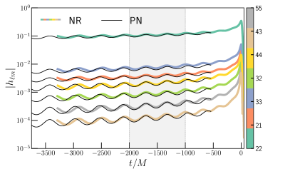
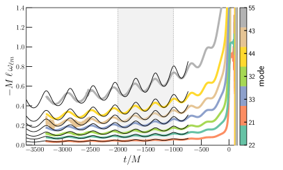
Figure 1: Amplitude and frequency of selected modes from an eccentric NR simulation (SXS:BBH:1364) together with an eccentric PN model are plotted. The PN model is evolved assuming a fixed value for initial eccentricity ($e_{0}=0.172$), mean anomaly ($l_{0}=2.681$) and the frequency dependent PN parameter ($x_{0}=0.0391$). The merger time of the NR waveform is set to zero. The initial set ($e_{0},l_{0},x_{0}$) is obtained by maximizing the overlap between the PN and NR waveform in a $1000M$ wide time-window, in a region where PN model is expected to agree with NR simulation. Additionally, a time shift is performed on the PN inspiral. The time-window of maximum overlap is shown as the shaded region. Binary’s component mass ratio ($q$) is 2, while the total mass ($M$) and the luminosity distance ($D_{\rm L}$) of the binary are set to $M$=1$M_{\odot}$ and $D_{\rm L}$=1Mpc respectively, following the convention of SXS simulations.

Finally, while a higher mode model can be constructed following the methods used in constructing the dominant mode model discussed in Sec. III, one may simply use the prescription for the ($\ell=2,|m|=2$) mode to combine an (eccentric) inspiral and a (quasi-circular) merger-ringdown prescription for each mode to obtain an ad hoc higher mode (HM) model as was done in Paper I. The alternate model presented in Sec. IV.1 is extended to include selected $\ell=|m|$ and $\ell-1=|m|$ modes and is validated against TEOBResumS-Dali Nagar et al. (2024b). These are the modes which are included in SEOBNRv5HM Pompili et al. (2023); the quasi-circular model used for the merger-ringdown part. Note also, these are also the modes for which we construct hybrids; see Fig. 3. The model is discussed in Sec. IV.2 and its performance is displayed in Fig. 11 for mildly inclined systems (30^∘).

The paper is structured in the following manner. In Sec. II we start by comparing waveforms from PN and NR approaches and discuss the construction of target hybrids. Next, in Sec. III we construct the waveform model by combining an eccentric PN inspiral model with a quasi-circular merger-ringdown model at a suitable point obtained by performing comparisons with target models. Subsequently, the model is validated against the target models not used in calibrating it as well as against an independent family of waveforms. In Sec. IV, we discuss an alternate model based on the prescriptions for attachment times obtained in Sec. III and subsequently extend this alternate model to include higher order modes. Finally, Sec. V presents summary of results and conclusions.

II Construction of target models with PN and NR inputs

Count	Simulation ID	$q$	$x_{0}$	$e_{0}$	$l_{0}$	$N_{\rm orb}$
Training Set
1	HYB:SXS:BBH:1355	1	0.0389	0.173	2.455	63.0
2	HYB:SXS:BBH:1356	1	0.0375	0.230	1.717	65.5
3	HYB:SXS:BBH:1358	1	0.0340	0.322	1.215	69.5
4	HYB:SXS:BBH:1359	1	0.0347	0.317	1.131	67.0
5	HYB:SXS:BBH:1360	1	0.0317	0.416	0.796	64.0
6	HYB:SXS:BBH:1361	1	0.0313	0.416	0.796	66.0
7	HYB:SXS:BBH:1364	2	0.0391	0.172	2.681	69.0
8	HYB:SXS:BBH:1365	2	0.0376	0.209	2.262	72.5
9	HYB:SXS:BBH:1366	2	0.0344	0.320	1.299	74.0
10	HYB:SXS:BBH:1367	2	0.0346	0.320	1.299	73.5
11	HYB:SXS:BBH:1368	2	0.0338	0.324	1.382	77.5
12	HYB:SXS:BBH:1372	3	0.0344	0.300	1.789	90.0
13	HYB:SXS:BBH:1373	3	0.0344	0.300	1.789	89.0
Testing Set
14	HYB:SXS:BBH:1357	1	0.0344	0.322	1.215	67.5
15	HYB:SXS:BBH:1362	1	0.0328	0.483	0.464	48.5
16	HYB:SXS:BBH:1363	1	0.0308	0.505	0.590	51.5
17	HYB:SXS:BBH:1369	2	0.0329	0.478	0.545	52.5
18	HYB:SXS:BBH:1370	2	0.0291	0.508	0.628	63.0
19	HYB:SXS:BBH:1371	3	0.0380	0.204	2.621	82.5
20	HYB:SXS:BBH:1374	3	0.0290	0.495	0.832	77.5

Table 1: Set of time-domain hybrids constructed by matching NR simulations from the SXS Catalog and state-of-the-art PN prescriptions for BBHs on eccentric orbits are listed. SXS simulation IDs are retained for identification with NR simulations used in constructing the hybrids. Each hybrid assumes a fixed value for initial eccentricity ($e_{0}$), mean anomaly ($l_{0}$) and the frequency dependent PN parameter ($x_{0}$) obtained using the gw_eccentricity package based on Ref. Shaikh et al. (2023). The PN parameter ($x$) is related to the GW frequency ($f_{\rm gw}$) of the dominant mode as $x$ =$(\pi Mf_{\rm gw})^{2/3}$ with $M$ representing binary’s total mass. Mass ratio ($q$) and number of orbits prior to the merger are also listed. $N_{\rm orb}$ is computed by taking the phase difference between the start of the waveform and the peak of the dominant mode ($\ell$=2, $|m|$=2) amplitude.

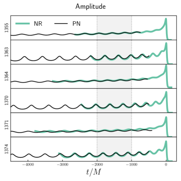
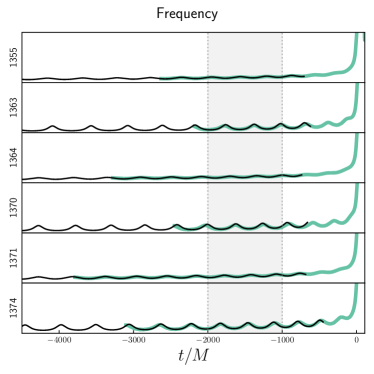
Figure 2: Same as Fig. 1, except that only dominant mode data is plotted and the comparison is shown for few other simulations with varying mass ratios and orbital parameters (see Table II for details). Initial values $(e_{0},l_{0},x_{0})$ with which the PN model is evolved for comparisons with various simulations are listed in Table II.

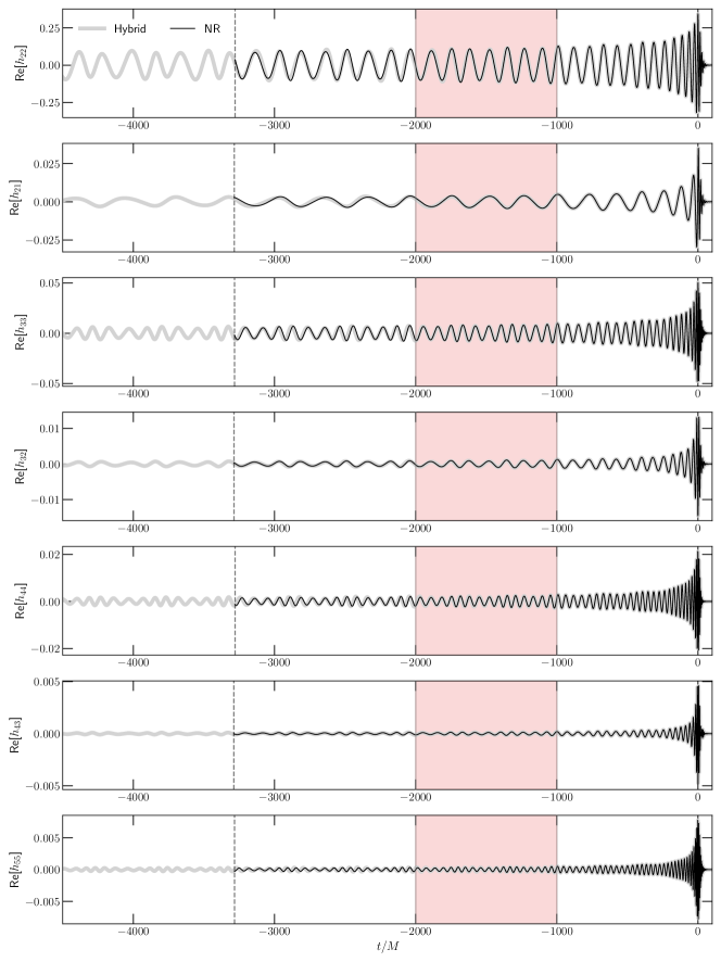
Figure 3: A hybrid model constructed by matching a NR simulation (SXS:BBH:1364) with a PN model (evolved using parameters consistent with the simulation) in a time-window where the two are expected to correctly predict the binary dynamics. For comparison the NR data is also plotted. The black dashed line marks the beginning of the NR waveform and the shaded light-red region $t\in(-2000M,-1000M)$ shows the matching window. Overlapping hybrid and NR waveforms on the left of the matching window hint at the quality of hybridization performed here. Table II lists details of all hybrids considered in the current work.

II.1 PN and NR comparisons

Paper I compares the PN inspiral waveforms with NR simulations. The inspiral mode amplitudes constituting 3PN inspiral waveforms assuming non-spinning binary systems on quasi-elliptical orbits were computed in Refs. Mishra et al. (2015); Boetzel et al. (2019); Ebersold et al. (2019). The orbital phase was taken from Ref. Tanay et al. (2016). GW frequency for each PN mode was obtained using the following scaling relation Ramos-Buades et al. (2022b)

$$\omega_{{}_{\ell m}}\sim\frac{m}{2}\times\omega_{\rm 22}\ .$$ (4)

NR simulations used in comparison with PN waveforms were produced using the Spectral Einstein Code (SpEC) developed by SXS collaboration and are publicly available Hinder et al. (2018); Boyle et al. (2019). Comparison of PN and NR prescriptions for a specific simulation was shown in Figure 1 of Paper I. Subsequently, a common region of validity was identified in which the two could be matched suitably to obtain hybrids listed in Table I there. (See Sec. III A-III C of Paper I for technical details).

Here too we aim to compare the PN and NR prescriptions leading to the construction of hybrids. While the hybridization method is same as in Paper I, comparison (which leads to identification of a suitable window for hybridization) is performed following a slightly different approach. In paper I, PN models were simply evolved to match a set of reference orbital parameters ($e_{\rm ref},l_{\rm ref}$) computed at a reference GW frequency ($x_{\rm ref}$) computed in Ref. Hinder et al. (2018) for each of the 20 simulations considered in Paper I. Here, we simply choose to compare the two waveforms in a $1000M$ wide time-window, slide it over the overlapping data and compute overlaps (the match maximized over a reference time and phase shifts; see Eq. (5) below) by varying ($e_{\rm ref},l_{\rm ref},f_{\rm ref}$) trio for the PN model, where $f_{\rm ref}$ is related to the PN parameter $x_{\rm ref}$ via $x_{\rm ref}$ =$(\pi Mf_{\rm ref})^{2/3}$. The match (${\mathcal{M}}$) between two waveforms is defined as an inner product given as

$$\mathcal{M}(\bm{\theta_{1},\theta_{2}})\equiv\mathrm{max}_{\phi_{\rm c},t_{\rm c}}\langle h(\bm{\theta_{1}}),h(\bm{\theta_{2}})e^{i(2\pi ft_{\rm c}-\phi_{\rm c})}\rangle\,,$$ (5)

with,

$$\langle h_{1},h_{2}\rangle\equiv 4\ \mathrm{Re}\left[\int_{0}^{\infty}df\frac{\tilde{h_{1}}^{*}(f)\tilde{h_{2}}(f)}{S_{h}(f)}\right]\,,$$ (6)

where $\langle h_{1},h_{2}\rangle$ represents the inner product between two waveforms $h_{1}$ and $h_{2}$ having unit norm and are functions of an intrinsic set of binary parameters ($\bm{\theta_{1},\theta_{2}}$). The phase $\phi_{\rm c}$, time $t_{\rm c}$ are measured at coalescence and $S_{h}(f)$ represents the noise in the detector (see Ref. Owen and Sathyaprakash (1999)).

We find the overlap is optimal for a time-window of ($-2000M$ to $-1000M$) and for a given ($e_{\rm ref},l_{\rm ref},f_{\rm ref}$) trio which becomes the starting reference ($e_{0}$, $l_{0}$, $f_{0}$) and may be different for different NR simulations (see Table II). Compared to the earlier approach, our current approach helps the construction of hybrids in at least two distinct ways. (1) The identification of hybridization window is done using quantitative measures such as overlaps and (2) the reference orbital parameters such as orbital eccentricity ($e_{0}$) and mean-anomaly ($l_{0}$) at a given frequency ($f_{0}$) will be free from gauge-ambiguities due to the use of the definition of Refs. Shaikh et al. (2023); Ramos-Buades et al. (2022b). With the suitable hybridization window identified, we can now proceed to reconstruct the hybrids.

Figure 1 compares the data corresponding to the NR simulation bearing simulation ID SXS:BBH:1364, for a selected set of modes chosen based on their relative significance compared to the dominant mode. PN model is evolved using a set of initial parameters ($e_{0}$, $l_{0}$, $f_{0}$) obtained using the procedure discussed above and then plotted together with the NR simulation after performing a time shift. The window giving maximum match is also displayed. For completeness we also show similar comparisons for few other simulations in Fig. 2 albeit for only the dominant mode. It is interesting to also note the time-window returning maximum match is common for all simulations.

II.2 Construction of hybrid waveforms

Complete IMR waveforms are constructed by matching PN and NR prescriptions for set of modes included in Fig. 1, in a region where the PN prescription closely mimics the NR data following the method of Ref. Varma and Ajith (2017). These are traditionally referred to as “hybrids”. As discussed in Ref. Varma and Ajith (2017), construction of hybrids including higher modes (in the circular case) is possible by performing at least two rotations (and a time shift) so as to align the frames in which PN/NR waveforms are defined. This argument was simply extended to the case of eccentric orbits in Paper I, assuming that the effect of marginalising over parameters such as eccentricity and mean anomaly will not significantly affect the hybridization. As discussed above, for the current work we simply adopt the hybridization procedure of Paper I. The prescription for construction of hybrids is discussed in detail in Ref. Varma and Ajith (2017) as well as in Paper I, nevertheless, we reproduce some of the steps here for completeness.

A least-squares minimization of the integrated difference between the GW modes from the PN and NR waveforms in a time interval ($t_{\rm i},t_{\rm f}$), in which the two approaches give similar results, is performed and can be defined as

$$\delta=\mathrm{min}_{t_{0},\varphi_{0},\psi}\int_{t_{\rm i}}^{t_{\rm f}}dt\sum_{\ell,m}\left|\mathpzc{h}_{\ell m}^{\mathrm{NR}}(t-t_{0})e^{i(m\varphi_{0}+\psi)}-\mathpzc{h}_{\ell m}^{\mathrm{PN}}(t)\right|,$$ (7)

where the minimization is performed over a time shift ($t_{0}$) and the two angles ($\varphi_{0},\psi$) as discussed above. The hybrid waveforms are then constructed by combining the NR data with the “best matched” PN waveform in the following way:

$$\mathpzc{h}_{\ell m}^{\mathrm{hyb}}(t)\equiv\,\tau(t)\,\mathpzc{h}_{\ell m}^{\mathrm{NR}}(t-t_{0}^{\prime})\ e^{i(m\varphi_{0}^{\prime}+\psi^{\prime})}+(1-\tau(t))\,\mathpzc{h}_{\ell m}^{\mathrm{PN}}(t),$$ (8)

where ($t_{0}^{\prime}$, $\varphi_{0}^{\prime}$, $\psi^{\prime}$) are the values of ($t_{0}$, $\varphi_{0}$, $\psi$) that minimize the integral of Eq. (7). In the above equation, $\tau(t)$ is a weighting function defined by

$$\tau(t)\equiv\left\{\begin{array}[]{ll}0&\textrm{if $t<t_{\rm i}$}\\ \frac{t-t_{\rm{i}}}{t_{\rm{f}}-t_{\rm{i}}}&\textrm{if $t_{\rm{i}}\leq t<t_{\rm{f}}$}\\ 1&\textrm{if $t_{\rm{f}}\leq t$.}\end{array}\right.$$ (12)

The hybrids corresponding to a representative NR simulation (SXS:BBH:1364) for all relevant modes are shown in Fig. 3. The two waveforms are aligned at merger and the shaded grey region $t\in(-2000M,-1000M)$ highlights the matching window where hybridization was performed. Overlapping hybrid and NR waveforms outside (on the left of) the matching window hint at the quality of hybridization performed here.

We reconstruct IMR hybrids corresponding to all $20$ eccentric NR simulations listed in Ref. Hinder et al. (2018) as was done for Paper I. These are listed in Table II and the SXS simulation IDs have been retained to identify the hybrids with the corresponding NR simulation. Each simulation starts with a specific initial eccentricity $(e_{0})$, mean anomaly ($l_{0}$) and frequency $(x_{0})$ obtained following the procedure discussed in Sec. II.1.

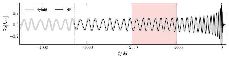
Figure 4: Same as Fig. 3 except, the PN part of the hybrid is purely based on EccentricTD model of Ref. Tanay et al. (2016). These are also the hybrids that are used in constructing and validating the model in Sec. III.

III The waveform model

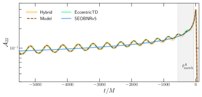
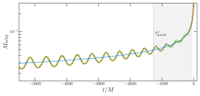
Figure 5: The (numerical) amplitude and frequency model produced by combining an eccentric inspiral with a quasi-circular merger-ringdown waveform for a total mass of 30$M_{\odot}$ is plotted against the hybrid used in calibrating the model. The eccentric inspiral (EccentricTD Tanay et al. (2016)) and the (quasi-circular) merger-ringdown (SEOBNRv5 Pompili et al. (2023)) models are also plotted for comparison. The amplitude (frequency) model transition smoothly from the inspiral to the merger-ringdown stage inside the shaded region(s), at $t_{\rm match}^{\mathcal{A}}$ ($t_{\rm match}^{\omega}$) values, maximizing the overlap between the model and the target hybrid.

Until now we focused on constructing a (PN-NR) hybrid model which could be used as a target for building a fully analytical IMR model for eccentric binary black hole mergers. While these hybrids could be used to construct the model following the procedure adopted in Paper I, as was done there, we construct an independent set of hybrids using PN model EccentricTD Tanay et al. (2016) (see Fig. 4). This is primarily done to minimize the difference between the target hybrids and the model (being constructed) that also uses the waveform EccentricTD Tanay et al. (2016) for the inspiral part. Note that, these new hybrids only include the dominant mode ($\ell=2,|m|=2$) since it is the dominant mode which we wish to model first. Note that, these are also the hybrids used in validating the model constructed in this section.

As in Paper I, here too we obtain a fully-analytical dominant ($\ell=2,|m|=2$) mode model by matching an eccentric PN inspiral Tanay et al. (2016) with a quasi-circular prescription for the merger-ringdown phase Pompili et al. (2023). Here too we stick to the procedures adopted in Paper I which involves identifying attachment times for both amplitude and frequency data together with an overall shift and the output is a coherent IMR model suitable for generating desired signals. Exact details concerning this model are outlined in Secs. III.1.1-III.1.3. Note however, that one must map the data for attachment times and time shifts to a set of physical parameters of the binary such as mass ratio and other relevant parameters. For $M\sim 25M_{\odot}$, the highest $x_{0}$ value of Table II corresponds to a frequency of $f\sim 20$Hz (low frequency cutoff for advanced LIGO design Aasi et al. (2015)). This motivates us to work with a conservative choice of $30M_{\odot}$ system when constructing the model. We find only 13 out of 20 cases reasonably agree (with overlaps $>$ 97%) for a $30M_{\odot}$ system with the hybrids and thus the final fits are obtained only using these 13 performing cases. Section III.2 discusses the details of construction of the analytical model.

III.1 Numerical Model

III.1.1 Time-shift

The process of generating a numerical model is similar to the procedure adopted in Paper I and we reproduce it here for clarity and completeness. As described in Sec. II.2, hybridization involves a minimization over a time shift, so when producing the amplitude model, we have to first perform a time shift of the inspiral waveform relative to the circular IMR waveform, because the time to merger is not known. This is done by first setting the merger time for the circular IMR waveform to zero and then time sliding the eccentric inspiral about the merger. We start by making a trial choice of $t_{\rm{shift}}$ and then generate an amplitude and a phase model by the methods described in Secs. III.1.2 and III.1.3, respectively.

III.1.2 Amplitude model

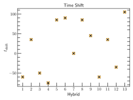
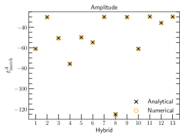
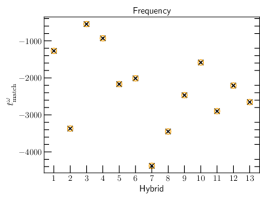
Figure 6: Numerical fits for $t_{\rm{match}}^{\mathcal{A}}$ and $t_{\rm{match}}^{\omega}$ as well as for $t_{\rm{shift}}$ are mapped into the physical parameter space for eccentric systems characterised by the binary’s eccentricity, mean anomaly at a reference frequency and the mass ratio parameter $q$ or $\eta$ depending upon the model best-fitting the data. Circles represent the numerical data points while crosses represent the value returned by the analytical best-fit model. The best-fit model(s) predict the numerical estimates for attachment times and the time-shift within $\pm 1M$.

As can be seen in Fig. 1, the waveforms tend to circularize near merger. Hence, in order to model this effect, we can join the eccentric inspiral to the circular IMR by suitable choice of an appropriate time $t_{\rm{match}}^{\mathcal{A}}$. The amplitude model is obtained by joining the eccentric inspiral with the circular IMR using a transition function over a time window of $500M$ which ends at $t_{\rm{match}}^{\mathcal{A}}$. Given a target hybrid, and a trial choice of $t_{\rm{shift}}$, we start with a trial choice of $t_{\rm{match}}^{\mathcal{A}}$ roughly $500M$ before the merger and produce the amplitude model as given below,

$$\mathcal{A}_{22}^{\mathrm{model}}(t)\equiv\,\tau_{\rm{a}}(t)\,\mathcal{A}_{22}^{\mathrm{IMR}}(t)\ +(1-\tau_{\rm{a}}(t))\,\mathcal{A}_{22}^{\mathrm{inspiral}}(t),$$ (13)

where $\tau_{\rm{a}}(t)$ is defined as

$$\tau_{\rm{a}}(t)\equiv\left\{\begin{array}[]{ll}0&\textrm{if $t<t_{\rm{i}}$}\\ \frac{t-t_{\rm{i}}}{t_{\rm{f}}-t_{\rm{i}}}&\textrm{if $t_{\rm{i}}\leq t<t_{\rm{f}}$}\\ 1&\textrm{if $t_{\rm{f}}\leq t$.}\end{array}\right.$$ (17)

We set $t_{\rm{i}}=t_{\rm{match}}^{\mathcal{A}}-500M$ and $t_{\rm{f}}=t_{\rm{match}}^{\mathcal{A}}$ as the bounds of the time interval over which the two waveforms are joined. Figure 5 demonstrates the process. The grey region is the time interval ending at $t_{\rm{match}}^{\mathcal{A}}$ where the inspiral and circular IMR is joined. After the amplitude model is obtained for a particular choice of trial $t_{\rm{shift}}$ and $t_{\rm{match}}^{\mathcal{A}}$, we combine it with the target hybrid phase to obtain the polarizations and then calculate the match with the target hybrid. We then change the trial choice of $t_{\rm{match}}^{\mathcal{A}}$ by $5M$, bringing it closer to the merger, and repeat the process of producing the amplitude model, and calculating the match. This variation of $t_{\rm{match}}^{\mathcal{A}}$ is done until roughly $30M$ before merger. We thus obtain a set of match values for varying $t_{\rm{match}}^{\mathcal{A}}$ but for a single trial $t_{\rm{shift}}$ and pick the one that has the highest value of match. We repeat the exercise for other choices of $t_{\rm{shift}}$ (trial $t_{\rm{shift}}$ varies between $-400M$ and $400M$ in steps of $5M$) and find out the corresponding $t_{\rm{match}}^{\mathcal{A}}$ with the highest value of match. Thus, we obtain a set of $t_{\rm{shift}}$ and $t_{\rm{match}}^{\mathcal{A}}$ pairs with a match value for each pair. From this set, the pair with the highest value of match is chosen as the numerical estimate for $t_{\rm{shift}}$ and $t_{\rm{match}}^{\mathcal{A}}$ for a particular target hybrid. We obtain numerical estimates using the same process for all 20 target hybrids.

III.1.3 Frequency model

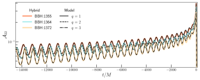
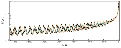
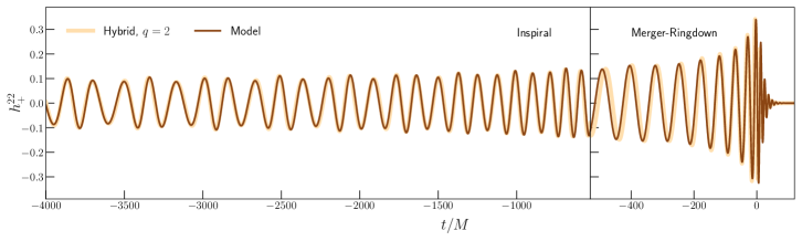
Figure 7: Top: Dominant mode ($\ell$=2, $|m|$=2) amplitude and frequency model, obtained by stitching an eccentric inspiral (EccentricTD Tanay et al. (2016)) with a quasi-circular merger-ringdown model (SEOBNRv5 Pompili et al. (2023)), at times predicted by the best-fit values of the (analytical) model are plotted against three representative target hybrids used in training the model. Bottom: one of the polarizations, obtained by combining the amplitude and the frequency model shown in the top panel for the $q=2$ case, is shown as a visual proof of the quality of the model being presented. The transition from inspiral to merger-ringdown is shown (for visual clarity) at $t_{\rm match}^{\mathcal{A}}$ given by Eq. (20) and has no impact on the plotted data.

For the frequency model, we follow a similar procedure as described in Sec. III.1.2 with the only difference being the duration of the time interval where the inspiral frequency is joined with the circular IMR frequency. The value of $t_{\rm{shift}}$ is fixed to the one that was obtained while producing the amplitude model. Similar to the amplitude model procedure, we determine an appropriate $t_{\rm{match}}^{\omega}$ for joining the inspiral frequency with the circular IMR frequency. However, the time interval where the two are joined, starts at $t_{\rm{match}}^{\omega}$ and ends at a time close to $30M$ before merger. Just like the amplitude model, we start with the choice of a trial value of frequency $t_{\rm{match}}^{\omega}$ roughly $6000M$ before merger and obtain the frequency model as given below,

$$\omega_{22}^{\mathrm{model}}(t)\equiv\,\tau_{\rm{a}}(t)\,\omega_{22}^{\mathrm{IMR}}(t)\ +(1-\tau_{\rm{a}}(t))\,\omega_{22}^{\mathrm{inspiral}}(t),$$ (18)

where $\tau_{\rm{a}}(t)$ is as defined in Eq. (17) with the difference being $t_{\rm{i}}=t_{\rm{match}}^{\omega}$ and $t_{\rm{f}}\lesssim-30M$. Figure 5 demonstrates the process. Once the frequency model is obtained for the choice of trial $t_{\rm{match}}^{\omega}$, we calculate the phase by integrating the frequency model. This is then combined with the amplitude model obtained for the same target hybrid (generated using the numerical estimate of $t_{\rm{shift}}$ and $t_{\rm{match}}^{\mathcal{A}}$ already obtained) to produce the polarizations and a match with the target hybrid is calculated. We then change the trial choice of $t_{\rm{match}}^{\omega}$ by $1M$, bringing it closer to the merger and repeat the process of producing the frequency model, and calculating the match. Once again, we do this variation until roughly $30M$ before merger to obtain a set of match values for varying $t_{\rm{match}}^{\omega}$ and pick the one that has the highest value of match. The corresponding value of frequency $t_{\rm{match}}^{\omega}$ is the numerical estimate for a particular target hybrid. We obtain numerical estimates for all 20 target hybrids using the same process.

III.2 Analytical model

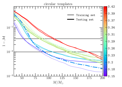
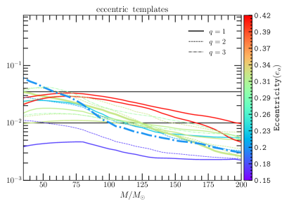
Figure 8: Mismatch as a function of total mass for all 13 training set hybrids (thin lines) and for the two testing set hybrids (HYB:SXS:BBH:1357 and HYB:SXS:BBH:1371; thick lines) when compared with dominant mode ($\ell$=2, $|m|$=$2$) quasi-circular templates (SEOBNRv5 Pompili et al. (2023); left panel) and eccentric templates (model constructed in Sec. III; right panel). The two horizontal lines indicate a match of 96.5% (or mismatch of 3.5%) and 99% (or 1% mismatch), respectively, and the color bar displays initial eccentricity ($e_{0}$) value at an initial GW frequency ($x_{0}$) for the respective target hybrid (see Table II).

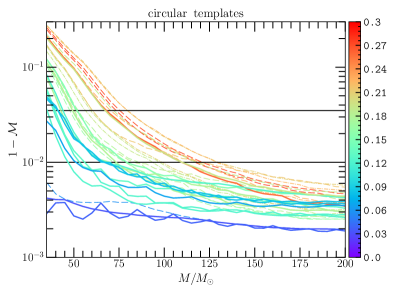
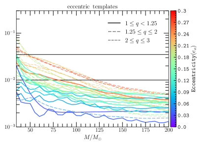
Figure 9: Same as Fig. 8 except mismatches are computed against an independent family of waveforms (TEOBResumS-Dali Nagar et al. (2024b)). Additionally, the parameter space explored by randomly sampling values for initial eccentricity ($e_{0}$) and mean anomaly ($l_{0}$) as well as of the mass ratio ($q$), in the range $0\lesssim e_{0}\lesssim 0.3$, $-\pi\leq l_{0}\leq\pi$, and $1\lesssim q\lesssim 3$, respectively.

We have described the procedure of producing (numerical) time-domain model fits for the dominant mode model, where we used a set of 20 eccentric hybrids as targets to calibrate our model. For each hybrid, we obtained a numerical estimate for $t_{\rm{shift}}$, $t_{\rm{match}}^{\mathcal{A}}$, and $t_{\rm{match}}^{\omega}$. In order to be able to generate waveforms for an arbitrary configuration these numerical fits need to be mapped into the physical parameter space for eccentric systems characterised by binary’s eccentricity, mean anomaly at a reference frequency and the mass ratio parameter. In this section, we determine a functional form by performing analytical fits to these numerical estimates. For analytical fits, we consider only those simulations (13 of the 20) for which the match between numerical model and the corresponding eccentric hybrid is greater than $97\%$ and collectively refer to them as training set and the remaining (7) simulations are categorized as testing set although only two of these (HYB:SXS:BBH:1357, 1371) can really be used to test the model as other simulations have initial eccentricities significantly larger than any of the training set hybrids and thus outside the calibration range for the model (See for instance, Table II). For this reason, when validating the model against hybrids we only include these two hybrids from testing set. The fitted functions obtained are of the form as mentioned below.

$$t_{\rm{shift}}\,(q,e,l) =\sum_{\alpha,\beta,\gamma,\delta}A_{\alpha\beta\gamma\delta}\,e^{\alpha}\,q^{\beta}\,\cos(\gamma\,l\,+\,\delta\,e\,l\,+\,a_{\alpha\beta\gamma\delta})\,,$$ (19)

for time shift, where $A_{\alpha\beta\gamma\delta}=a_{\alpha\beta\gamma\delta}=0$ for $\alpha+\beta>3$ and/or $\alpha>2$ and/or $\gamma+\delta>1$, and $A_{\alpha 001}=A_{0\beta 10}=A_{0\beta 01}=A_{00\gamma\delta}=a_{\alpha\beta 00}=0$,

$$t_{\rm{match}}^{\mathcal{A}}\,(\eta,e,l) =\sum_{\alpha,\beta,\gamma,\delta}B_{\alpha\beta\gamma\delta}\,e^{\alpha}\,\eta^{\beta}\,\cos(\gamma\,l\,+\,\delta\,e\,l\,+\,b_{\alpha\beta\gamma\delta})\,,$$ (20)

for amplitude, where $B_{\alpha\beta\gamma\delta}=b_{\alpha\beta\gamma\delta}=0$ for $\alpha+\beta>3$ and/or $\alpha>2$ and/or $\gamma+\delta>1$, and $B_{0\beta 10}=B_{0\beta 01}=B_{00\gamma\delta}=b_{\alpha\beta 00}=0$, and

$$t_{\rm{match}}^{\omega}\,(\eta,e,l) =\sum_{\alpha,\beta,\gamma,\delta}C_{\alpha\beta\gamma\delta}\,e^{\alpha}\,\eta^{\beta}\,\cos(\gamma\,l\,+\,\delta\,e\,l\,+\,c_{\alpha\beta\gamma\delta})\,,$$ (21)

for frequency, where $C_{\alpha\beta\gamma\delta}=c_{\alpha\beta\gamma\delta}=0$ for $\alpha+\beta>3$ and/or $\alpha>2$ and/or $\gamma+\delta>1$, and $C_{0\beta 10}=C_{0\beta 01}=C_{00\gamma\delta}=c_{\alpha\beta 00}=0$. The values for the coefficients $A_{\alpha\beta\gamma\delta}$, $B_{\alpha\beta\gamma\delta}$, $C_{\alpha\beta\gamma\delta}$, $a_{\alpha\beta\gamma\delta}$, $b_{\alpha\beta\gamma\delta}$, and $c_{\alpha\beta\gamma\delta}$ obtained by performing a fit to the numerical values are tabulated in Tables II-II. Figure 6 shows comparisons between the numerically obtained values for $t_{\rm{shift}}$, $t_{\rm{match}}^{\mathcal{A}}$, and $t_{\rm{match}}^{\omega}$, with the values predicted by our analytical fits. The predictions are within $\pm 1M$ for numerical estimates for $t_{\rm shift}$, $t_{\rm{match}}^{\mathcal{A}}$ and $t_{\rm{match}}^{\omega}$. We show amplitude and frequency comparison between the target hybrids and our models for three cases along with the full waveform for the $q=2$ case in Fig. 7.

III.3 Validation

The performance of the model can be assessed from the plots against the new hybrids presented in Fig. 7, as well as from the mismatch ($1-\mathcal{M}$) plots displayed in Fig. 8. Note again, the new hybrids are purely based on the PN prescription, EccentricTD Tanay et al. (2016) – the same model that constitutes the inspiral part of the model constructed here. Certainly, the dominant mode model outperforms the quasi-circular templates. On top of that, unlike Paper I, the model provides $\geq 96.5\%$ match against all the training set hybrids for almost the entire range of parameters considered here. Furthermore, we also try to test our model against the testing set hybrids using Nelder-Mead down-hill simplex minimization algorithm of Scipy Oliphant and Contributors (2020) over the three initial parameters set ($e_{0},l_{0},f_{0}$) for each testing set hybrid. The mismatch against testing hybrids are plotted as thick lines in both panels of Fig. 8. As can be seen there, for $q=1$ (testing) hybrid, match is $\geq 96.5\%$ for the entire range of total mass, while it degrades a little for $q=3$ (testing) hybrid for the low mass range ($M\lesssim 60M_{\odot}$) which is consistent with the trends observed for mismatch against $q=3$ training set simulations.

Note that the target hybrids used in these mismatch computations include only the ($\ell=2,|m|=2$) mode so as to assess the actual performance of the dominant mode model. Given the quality of analytical fits it is not surprising that the analytical model performs well against the set of hybrids used in training the model. Moreover, we retain the cases agreeing closely with the hybrids apart from two testing hybrids. (Only 13 out of 20 simulations were used in finding the analytical model.) Keeping this in mind we also try to test our model against an independent waveform family TEOBResumS-Dali Nagar et al. (2024b). For this comparison, we choose to sample a parameter space that is not identical to the training set hybrids. We choose to randomly sample the values of a reference eccentricity ($e_{0}$), mass ratio ($q$) and reference mean anomaly ($l_{0}$) in the range $0\lesssim e_{0}\lesssim 0.3$, $1\lesssim q\lesssim 3$ and $-\pi\leq l_{0}\leq\pi$, respectively. Note that the range for initial orbital eccentricity ($e_{0}$) is slightly different from the ones spanned by the hybrids. While the upper value is chosen conservatively to take $e_{0}=0.3$ to reduce any systematic differences between the model and the waveform TEOBResumS-Dali Nagar et al. (2024b) at large eccentricity values, near circular cases are also included to see if the model gradually produces the circular limit despite being trained on purely eccentric target models.

Next, the template (dominant eccentric model) is optimized against the target (TEOBResumS-Dali Nagar et al. (2024b)) using the same minimization algorithm Oliphant and Contributors (2020) used in validating the model against testing set hybrids. The mismatch plot obtained is shown in Fig. 9. Additionally, for comparison, mismatches of TEOBResumS-Dali Nagar et al. (2024b) with quasi-circular SEOBNRv5 Pompili et al. (2023) templates are displayed in the left panel. Clearly, our model seems to do better compared to the circular templates at the low mass end where the overlaps are $\gtrsim$ 96.5% for nearly the entire range of parameters considered in the comparison. The mismatches are comparable for heavier systems as expected.

IV An alternate model and inclusion of higher modes

IV.1 Eccentric model based on TaylorT2 phase and PN corrected amplitudes

In this section, we discuss the possibility of finding a suitable alternative to the model constructed in the previous section. As mentioned earlier in the Sec. I.2, we propose to replace the PN model used in constructing the model in the previous section to include amplitude terms with higher PN accuracy in the model. We employ 3PN accurate expressions for the dominant mode amplitude of Refs. Mishra et al. (2015); Boetzel et al. (2019); Ebersold et al. (2019) and a 3PN accurate phasing (based on TaylorT2 approximant) Moore et al. (2016) to construct this alternate model. Note that the inspiral part of the model presented in Sec. III was entirely based on the work of Ref. Tanay et al. (2016). The EccentricTD approximant is 2PN accurate in phase and only Newtonian accurate in amplitude for the eccentricity related effects although is based on a superior (compared to TaylorT2) approximant namely TaylorT4 and should also work better for larger eccentricities as it includes corrections to 6th power in eccentricity while the TaylorT2 phase we use involves only leading order corrections of eccentricity although is 3PN accurate Moore et al. (2016). To test the performance of this model, we again compare this model with TEOBResumS-Dali Nagar et al. (2024b) by computing overlaps on the same set of parameters used in validating the dominant mode model in Sec. III.3. The results are shown in Fig. 10. Overlaps between the model and the target waveforms are better than $\sim 96.5\%$ for almost the entire range considered here, making it a suitable alternative to the presented EccentricTD model.

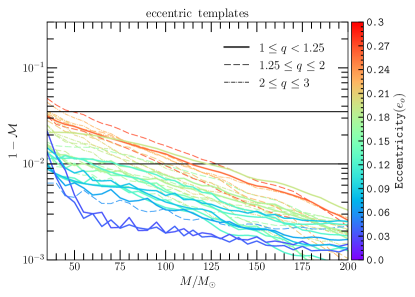
Figure 10: Same as in Fig. 9 except target waveforms (TEOBResumS-Dali Nagar et al. (2024b)) are compared with the alternate dominant mode model presented in Sec. IV.1.

IV.2 Inclusion of higher order modes

In this section, we extend the dominant mode model of Sec. IV.1 to obtain a higher mode model by including ($\ell$, $|m|$)=(2, 2), (2, 1), (3, 3), (3, 2), (4, 4), (4, 3) and (5, 5) modes. These are precisely the modes which are included in SEOBNRv5HM(Ref. Pompili et al. (2023)) which we use for the merger-ringdown part and also included in the hybrids constructed in Sec. II.2. The (eccentric) inspiral and (quasi-circular) merger-ringdown models are again attached using the analytical expressions for $t_{\rm{shift}}$, $t_{\rm{match}}^{\mathcal{A}}$ and $t_{\rm{match}}^{\omega}$, obtained for the dominant mode model in Sec. III. (The higher mode model of Paper I was also obtained following the same strategy albeit, the HM model there only included the $\ell=|m|$ modes.) The inspiral part of the model for each non-quadrupole mode is obtained by combining the mode amplitudes obtained in Refs. Mishra et al. (2015); Boetzel et al. (2019); Ebersold et al. (2019) and orbital frequency (multiplied by an appropriate factor involving mode number; see Eq. (4)). Figure 11 compares our higher mode model against the HM version of the waveform, TEOBResumS-Dali Nagar et al. (2024b). While all modes up to $\ell=8$ are included in TEOBResumS-Dali, we choose to include the same set of modes in the target and the model waveform to control the systematics. The orbital inclination angle is chosen to be $30^{\circ}$. We find that the higher mode model recovers the target waveforms with accuracy better than $96.5\%$ for nearly the entire range of parameter values considered here and thus may be used for analysing signals containing non-quadrupole modes and inclination angles $\leq 30^{\circ}$.

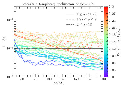
Figure 11: Similar to Fig. 10 except, that both the target and the model now include all modes included in our hybrids and the inclination angle of the binary is chosen to be $30^{\circ}$.

IV.3 Recovery of aligned spin binaries

Although our alternate model (including higher modes) is nonspinning, we also test its performance against a spinning model for a few mildly spinning cases. We assume spin-precession to be absent and thus binary’s spin is described solely by the effective spin parameter, $\chi_{\rm eff}$. When expressed in terms of dimensionless spin components, $\chi_{i}=(\vec{S_{i}}\cdot\hat{L})/m_{i}^{2}$, it reads Divyajyoti et al. (2024b); Ajith et al. (2011); Santamaria et al. (2010)

$$\chi_{\rm eff}=\frac{\chi_{1}m_{1}+\chi_{2}m_{2}}{m_{1}+m_{2}}\,.$$ (22)

Here, $m_{i}$ refers to the mass of the binary component having spin angular momentum $\vec{S_{i}}$, and $\hat{L}$ denotes the unit vector along the direction of the orbital angular momentum of the binary.

Figure 12 compares our nonspinning model with the spinning version of TEOBResumS-Dali Nagar et al. (2024b). Thick curves represent the mismatch when the inclination angle ($\iota$) is set to zero for which only $|m|=2$ modes survive (in our case (2, 2) and (3, 2)). Thin lines on the other hand, show mismatches for the inclination angle of $30^{\circ}$ and thus display mismatches with all $\ell=|m|$ and $\ell-1=|m|$ modes included in our higher mode model. For the equal mass case ($q=1$), we find excellent agreements with target models (matches $\gtrsim 99\%$). For $q=2$ case, the matches are still $\gtrsim 96.5\%$ for $\chi_{\rm{eff}}\leq 0.1$ for all systems with $M\gtrsim 60M_{\odot}$. This clearly shows that despite being nonspinning in nature, the model could be used to analyse mildly spinning events observed routinely by current generation detectors such as LIGO and Virgo Abbott et al. (2019c, 2021d, 2023). In other words, systematics due to neglect of spin effects may be ignored.

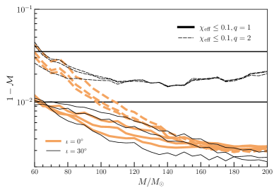
Figure 12: Recovery of mildly spinning target waveforms (TEOBResumS-Dali Nagar et al. (2024b)) with the alternate nonspinning model presented in Sec. IV.1 is displayed for two different mass ratio cases ($q=1$, 2) and a set of effective spin values (with $\chi_{\rm eff}\leq 0.1$).

V Discussion and conclusion

Our current work is a follow up of our earlier work of Ref. Chattaraj et al. (2022) (referred as Paper I through preceding sections) where we developed a fully analytical dominant mode model for nonspinning binary black holes on elliptical orbits. The model was obtained by stitching an eccentric inspiral EccentricTD Tanay et al. (2016) with a quasi-circular merger ringdown prescription SEOBNRv4 Bohé et al. (2017). Here, we revisit the construction of the model presented in Paper I following a new definition of orbital eccentricity presented in Refs. Shaikh et al. (2023); Ramos-Buades et al. (2022b).

We started by comparing 20 distinct NR simulations from SXS collaboration presented in Ref. Hinder et al. (2018) with a PN prescription obtained by combing the results of Refs. Ebersold et al. (2019); Boetzel et al. (2017); Tanay et al. (2016) for a selected set of modes chosen based on their relative significance compared to the dominant modes. Figure 1 shows a comparison of the amplitude and frequency data for one particular dataset. The PN model is evolved using an initial set of binary orbital parameters such as orbital eccentricity consistent with the definition of Refs. Shaikh et al. (2023); Ramos-Buades et al. (2022b). For completeness, we also show dominant mode comparisons for few other simulations in Fig. 2. We find that the PN and NR prescriptions have maximum overlap in a time-window of ($-2000M,-1000M$) shown by shaded regions of Fig. 1-2. In fact, we observe a minimum match of $\sim$ 96% for all 20 simulations sets against PN models in this window, allowing hybridization of the two in this window. Table II lists all hybrids constructed here. Figure 3 displays one of these hybrids and as shown there the hybrid are constructed for all modes included in the comparison presented in Fig. 1. The hybridization procedure is same as in Paper I and is reproduced in Sec. II.2. However, the model constructed in Sec. III is trained, following Paper I, with a new set of dominant mode hybrids, which uses the same PN prescription used in our dominant mode model. Details of model construction is discussed in Sec. III.1-III.2 and validation is performed in Sec. III.3.

We validate the model against the hybrids used in training the model (training set in Table II) as well as two simulations (HYB:SXS:BBH:1357, 1371) from the testing set. While consistency with training set was expected (but also confirms the quality of fits), better than $96.5\%$ match with the two testing set simulations for most of the parameter space confirm the reliability of the model (see thick curves in the right panel of Fig. 8). Clearly the model also outperforms quasi-circular model shown in the left panel of Fig. 8. We also validate the model against an independent waveform family TEOBResumS-Dali Nagar et al. (2024b) for values randomly sampled for initial values of eccentricity ($e_{0}$), mass ratio ($q$), and mean anomaly ($l_{0}$) in the range $0\lesssim e_{0}\lesssim 0.3$, $1\lesssim q\lesssim 3$, and $-\pi\leq l_{0}\leq\pi$, respectively. Note the difference in eccentricity scale explored here compared to the one in Fig. 8 (See, Sec. III.3 for a discussion). Figure 9 shows this comparison and the model recovers the target family with overlaps better than $96.5\%$ for mass ratios $\leq 1.25$. For $q>1.25$, mismatches are slightly poorer for cases with $M\leq 50M_{\odot}$.

We also provide an alternate model by combining PN inputs from Ref. Moore et al. (2016) and Refs. Mishra et al. (2015); Boetzel et al. (2019); Ebersold et al. (2019) for phase and amplitude part of the model respectively. The performance of this model against the waveform used in validating the model in Fig. 9 has been shown in Fig. 10. As can be seen, the performance of this alternate model is at the same level as of the model presented in Sec. III. Further, following Paper I, we also extended this alternate model to include few leading $\ell$=$|m|$ and $\ell-1$=$|m|$ modes (up to $\ell=5$) and compare it against waveforms of TEOBResumS-Dali Nagar et al. (2024b) in Fig. 11 keeping the same set of modes in both target and template. As we can see the model at least reliably reproduces the target model for inclination angles $\leq 30^{\circ}$.

Finally, while our model(s) assumes spinless binary constituents, we also tried testing its suitability for analysing signals with small spin magnitudes in the absence of spin precession. Figure 12 compares our nonspinning model (including higher modes) presented in Sec. IV.1-IV.2 against the HM model of TEOBResumS-Dali Nagar et al. (2024b) (with spins switched on). As shown there, our model seems to be able to extract the equal mass spinning target waveforms with accuracy better than $99\%$ as shown by the thick-solid lines. On the other hand, our model recover target model with matches larger than than 96.5% for the $q=2$ case (thin-dashed lines). For higher spin magnitudes as well as higher mass ratios, mismatches are larger than 3.5% in the low mass range, at least for unequal mass cases.

Note that, both the alternate model as well as the HM model were not obtained by calibrating against hybrids but rather we simply used the prescriptions presented in context of dominant mode model in Sec. III.2 and thus could be improved, however we restrict ourselves here to a proof of principle demonstration that alternate prescriptions for dominant mode model as well as simple extensions like the one proposed here could be easily achieved and perform reliably and leave such updates for a future work. Apart from being able to construct an improved model compared to the one presented in Paper I, in the current work we also address a few concerns with the model there. First, it was found that for nearly 10-15% cases, the analytical fits for times for merger-ringdown attachment produced nonphysical values (beyond merger at $t>0$). Since the NR simulations used in this work essentially circularize by $30M$ before the merger Hinder et al. (2018), we impose this condition for those nonphysical scenarios. This removes the discrepancy regarding the attachment times and ensures the validity of the model in the entire parameter space explored. Secondly, the model presented in Sec. IV.1 is significantly faster than the dominant mode model of Paper I. This is likely due to a speedup with merger-ringdown model (SEOBNRv5 Pompili et al. (2023) instead of SEOBNRv4 Bohé et al. (2017)). The waveform generation rate of TaylorT2 model is $\sim 1.5$ times higher than the model based on EccentricTD. Moreover, when compared with the waveform TEOBResumS-Dali Nagar et al. (2024b), these waveforms nearly have a $\sim 2$ times speedup and thus likely to be useful for parameter estimation studies.

VI Acknowledgments

We thank Kaushik Paul and Prayush Kumar for sharing invaluable insights in validating our model. We thank the authors of Ref. Nagar et al. (2024b) for making the implementation of the TEOBResumS-Dali available for public use teo , and Divyajyoti for helping us with technical details of the implementation and waveform generation. We are thankful to the SXS Collaboration for making a public catalog of numerical relativity waveforms. P.M. thanks the members of the gravitational wave group at the Department of Physics, IIT Madras for organizing the weekly journal club sessions and the insightful discussions. T.R.C. acknowledges the support of the National Science Foundation award PHY-2207728. C.K.M. acknowledges the support of SERB’s Core Research Grant No. CRG/2022/007959. This document has LIGO preprint number LIGO-P2400355. We thank Md Arif Shaikh for useful comments and suggestions on our manuscript.

Appendix A Coefficients of the analytical fit

Here we tabulate the coefficients of the analytical fits for the parameters $t_{\rm shift},t_{\rm match}^{\mathcal{A}}$ and $t_{\rm match}^{\omega}$ obtained in Sec III.2. The expressions are given in Eq. (19), (20) and (21).

$\alpha\beta\gamma\delta$	$A_{\alpha\beta\gamma\delta}$	$a_{\alpha\beta\gamma\delta}$
$1010$	$-2030.2$	$-5.38518$
$1101$	$250.49$	$1.04693$
$2010$	$6608.44$	$-18.0212$

Table 2: Table of coefficients for the analytical expression of $t_{\rm{shift}}$ in Eq. (19). All other coefficients not included in the table are zero.

$B_{\alpha\beta 00}$	$\beta=0$	1	2
$\alpha=0$	$24215.3$	$-120939.0$	$91243.2$
1	$-166056.$	$673029.$	$0$
2	$328096.$	$-1.34817\times 10^{6}$	$0$

Table 3: Table of coefficients for the analytical expression of amplitude $t_{\rm{match}}$ in Eq. (20). All other coefficients not included in the table are zero.

$C_{\alpha\beta 00}$	$\beta=0$	1	2
$\alpha=0$	$-1.87711\times 10^{6}$	$8.92879\times 10^{6}$	$-5.75326\times 10^{6}$
1	$1.30607\times 10^{7}$	$-5.21053\times 10^{7}$	$0$
2	$-2.51977\times 10^{7}$	$1.04979\times 10^{8}$	$0$

Table 4: Table of coefficients for the analytical expression of frequency $t_{\rm{match}}$ in Eq. (21). All other coefficients not included in the table are zero.

References

- Chattaraj et al. (2022) A. Chattaraj, T. RoyChowdhury, Divyajyoti, C. K. Mishra, and A. Gupta, Phys. Rev. D 106, 124008 (2022), arXiv:2204.02377 [gr-qc] .
- Abbott et al. (2016a) B. P. Abbott et al. (LIGO Scientific, Virgo), Phys. Rev. Lett. 116, 061102 (2016a), arXiv:1602.03837 [gr-qc] .
- Abbott et al. (2019a) B. P. Abbott et al. (LIGO Scientific and Virgo Collaborations), Phys. Rev. X 9, 031040 (2019a), arXiv:1811.12907 [astro-ph.HE] .
- Abbott et al. (2021a) R. Abbott et al. (LIGO Scientific, Virgo), Phys. Rev. X 11, 021053 (2021a), arXiv:2010.14527 [gr-qc] .
- Abbott et al. (2021b) R. Abbott et al. (LIGO Scientific, VIRGO), Phys. Rev. D 109, 022001 (2021b), arXiv:2108.01045 [gr-qc] .
- Abbott et al. (2021c) R. Abbott et al. (LIGO Scientific, VIRGO, KAGRA), (2021c), arXiv:2111.03606 [gr-qc] .
- (7) https://gwosc.org/eventapi/html/allevents/.
- Abbott et al. (2016b) B. P. Abbott et al. (LIGO Scientific, Virgo), Astrophys. J. Lett. 818, L22 (2016b), arXiv:1602.03846 [astro-ph.HE] .
- Abbott et al. (2020a) R. Abbott et al. (LIGO Scientific, Virgo), Astrophys. J. Lett. 900, L13 (2020a), arXiv:2009.01190 [astro-ph.HE] .
- Abac et al. (2023) A. G. Abac et al. (LIGO Scientific, VIRGO, KAGRA), (2023), arXiv:2308.03822 [astro-ph.HE] .
- Abbott et al. (2016c) B. P. Abbott et al. (LIGO Scientific, Virgo), Phys. Rev. Lett. 116, 221101 (2016c), [Erratum: Phys.Rev.Lett. 121, 129902 (2018)], arXiv:1602.03841 [gr-qc] .
- Zevin et al. (2019) M. Zevin, J. Samsing, C. Rodriguez, C.-J. Haster, and E. Ramirez-Ruiz, Astrophys. J. 871, 91 (2019), arXiv:1810.00901 [astro-ph.HE] .
- Ramos-Buades et al. (2020a) A. Ramos-Buades, S. Tiwari, M. Haney, and S. Husa, Phys. Rev. D 102, 043005 (2020a), arXiv:2005.14016 [gr-qc] .
- Fumagalli et al. (2024) G. Fumagalli, I. Romero-Shaw, D. Gerosa, V. De Renzis, K. Kritos, and A. Olejak, (2024), arXiv:2405.14945 [astro-ph.HE] .
- Peters (1964) P. C. Peters, Phys. Rev. 136, B1224 (1964).
- Aasi et al. (2015) J. Aasi et al. (LIGO Scientific), Class. Quant. Grav. 32, 074001 (2015), arXiv:1411.4547 [gr-qc] .
- Acernese (2015) F. Acernese (Virgo), J. Phys. Conf. Ser. 610, 012014 (2015).
- Abbott et al. (2019b) B. P. Abbott et al. (LIGO Scientific, Virgo), Astrophys. J. 883, 149 (2019b), arXiv:1907.09384 [astro-ph.HE] .
- Abbott et al. (2020b) R. Abbott et al. (LIGO Scientific, Virgo), Phys. Rev. Lett. 125, 101102 (2020b), arXiv:2009.01075 [gr-qc] .
- Gamba et al. (2023) R. Gamba, M. Breschi, G. Carullo, S. Albanesi, P. Rettegno, S. Bernuzzi, and A. Nagar, Nature Astron. 7, 11 (2023), arXiv:2106.05575 [gr-qc] .
- Kimball et al. (2021) C. Kimball et al., Astrophys. J. Lett. 915, L35 (2021), arXiv:2011.05332 [astro-ph.HE] .
- Romero-Shaw et al. (2021) I. M. Romero-Shaw, P. D. Lasky, and E. Thrane, Astrophys. J. Lett. 921, L31 (2021), arXiv:2108.01284 [astro-ph.HE] .
- O’Shea and Kumar (2023) E. O’Shea and P. Kumar, Phys. Rev. D 108, 104018 (2023), arXiv:2107.07981 [astro-ph.HE] .
- Romero-Shaw et al. (2022) I. M. Romero-Shaw, P. D. Lasky, and E. Thrane, Astrophys. J. 940, 171 (2022), arXiv:2206.14695 [astro-ph.HE] .
- Iglesias et al. (2022) H. L. Iglesias et al., (2022), arXiv:2208.01766 [gr-qc] .
- Gupte et al. (2024) N. Gupte et al., (2024), arXiv:2404.14286 [gr-qc] .
- Brown and Zimmerman (2010) D. A. Brown and P. J. Zimmerman, Phys. Rev. D 81, 024007 (2010), arXiv:0909.0066 [gr-qc] .
- Huerta and Brown (2013) E. A. Huerta and D. A. Brown, Phys. Rev. D 87, 127501 (2013), arXiv:1301.1895 [gr-qc] .
- Favata et al. (2022) M. Favata, C. Kim, K. G. Arun, J. Kim, and H. W. Lee, Phys. Rev. D 105, 023003 (2022), arXiv:2108.05861 [gr-qc] .
- Abbott et al. (2017a) B. P. Abbott et al. (LIGO Scientific, Virgo), Class. Quant. Grav. 34, 104002 (2017a), arXiv:1611.07531 [gr-qc] .
- Divyajyoti et al. (2024a) Divyajyoti, S. Kumar, S. Tibrewal, I. M. Romero-Shaw, and C. K. Mishra, Phys. Rev. D 109, 043037 (2024a), arXiv:2309.16638 [gr-qc] .
- McClelland et al. (2016) D. McClelland, M. Evans, R. Schnabel, B. Lantz, I. Martin, and V. Quetschke, (2016).
- Dwyer et al. (2015) S. Dwyer, D. Sigg, S. W. Ballmer, L. Barsotti, N. Mavalvala, and M. Evans, Phys. Rev. D 91, 082001 (2015), arXiv:1410.0612 [astro-ph.IM] .
- Abbott et al. (2017b) B. P. Abbott et al. (LIGO Scientific), Class. Quant. Grav. 34, 044001 (2017b), arXiv:1607.08697 [astro-ph.IM] .
- Punturo et al. (2010) M. Punturo et al., Class. Quant. Grav. 27, 194002 (2010).
- Hild et al. (2011) S. Hild et al., Class. Quant. Grav. 28, 094013 (2011), arXiv:1012.0908 [gr-qc] .
- Lower et al. (2018) M. E. Lower, E. Thrane, P. D. Lasky, and R. Smith, Phys. Rev. D 98, 083028 (2018), arXiv:1806.05350 [astro-ph.HE] .
- (38) S. Tibrewal et al., In preparation (2022).
- Mishra et al. (2015) C. K. Mishra, K. G. Arun, and B. R. Iyer, Phys. Rev. D 91, 084040 (2015), arXiv:1501.07096 [gr-qc] .
- Moore et al. (2016) B. Moore, M. Favata, K. Arun, and C. K. Mishra, Phys. Rev. D 93, 124061 (2016), arXiv:1605.00304 [gr-qc] .
- Tanay et al. (2016) S. Tanay, M. Haney, and A. Gopakumar, Phys. Rev. D 93, 064031 (2016), arXiv:1602.03081 [gr-qc] .
- Boetzel et al. (2019) Y. Boetzel, C. K. Mishra, G. Faye, A. Gopakumar, and B. R. Iyer, Phys. Rev. D 100, 044018 (2019), arXiv:1904.11814 [gr-qc] .
- Ebersold et al. (2019) M. Ebersold, Y. Boetzel, G. Faye, C. K. Mishra, B. R. Iyer, and P. Jetzer, Phys. Rev. D 100, 084043 (2019), arXiv:1906.06263 [gr-qc] .
- Königsdörffer and Gopakumar (2006) C. Königsdörffer and A. Gopakumar, Phys. Rev. D 73, 124012 (2006), arXiv:gr-qc/0603056 [gr-qc] .
- Moore and Yunes (2019) B. Moore and N. Yunes, Class. Quant. Grav. 36, 185003 (2019), arXiv:1903.05203 [gr-qc] .
- Carullo et al. (2024) G. Carullo, S. Albanesi, A. Nagar, R. Gamba, S. Bernuzzi, T. Andrade, and J. Trenado, Phys. Rev. Lett. 132, 101401 (2024), arXiv:2309.07228 [gr-qc] .
- Carullo (2024) G. Carullo, (2024), arXiv:2406.19442 [gr-qc] .
- Hinder et al. (2018) I. Hinder, L. E. Kidder, and H. P. Pfeiffer, Phys. Rev. D 98, 044015 (2018), arXiv:1709.02007 [gr-qc] .
- Huerta et al. (2017) E. A. Huerta et al., Phys. Rev. D 95, 024038 (2017), arXiv:1609.05933 [gr-qc] .
- Chen et al. (2021) Z. Chen, E. A. Huerta, J. Adamo, R. Haas, E. O’Shea, P. Kumar, and C. Moore, Phys. Rev. D 103, 084018 (2021), arXiv:2008.03313 [gr-qc] .
- Setyawati and Ohme (2021) Y. Setyawati and F. Ohme, Phys. Rev. D 103, 124011 (2021), arXiv:2101.11033 [gr-qc] .
- Gamba et al. (2024) R. Gamba, D. Chiaramello, and S. Neogi, (2024), arXiv:2404.15408 [gr-qc] .
- Ramos-Buades et al. (2020b) A. Ramos-Buades, S. Husa, G. Pratten, H. Estellés, C. García-Quirós, M. Mateu-Lucena, M. Colleoni, and R. Jaume, Phys. Rev. D 101, 083015 (2020b), arXiv:1909.11011 [gr-qc] .
- Chiaramello and Nagar (2020) D. Chiaramello and A. Nagar, Phys. Rev. D 101, 101501 (2020), arXiv:2001.11736 [gr-qc] .
- Albertini et al. (2024) A. Albertini, R. Gamba, A. Nagar, and S. Bernuzzi, Phys. Rev. D 109, 044022 (2024), arXiv:2310.13578 [gr-qc] .
- Nagar and Albanesi (2022) A. Nagar and S. Albanesi, Phys. Rev. D 106, 064049 (2022), arXiv:2207.14002 [gr-qc] .
- Nagar et al. (2024a) A. Nagar, R. Gamba, P. Rettegno, V. Fantini, and S. Bernuzzi, (2024a), arXiv:2404.05288 [gr-qc] .
- Nagar et al. (2024b) A. Nagar, S. Bernuzzi, D. Chiaramello, V. Fantini, R. Gamba, M. Panzeri, and P. Rettegno, (2024b), arXiv:2407.04762 [gr-qc] .
- Abbott et al. (2019c) B. P. Abbott et al. (LIGO Scientific, Virgo), Astrophys. J. Lett. 882, L24 (2019c), arXiv:1811.12940 [astro-ph.HE] .
- Abbott et al. (2021d) R. Abbott et al. (LIGO Scientific, Virgo), Astrophys. J. Lett. 913, L7 (2021d), arXiv:2010.14533 [astro-ph.HE] .
- Abbott et al. (2023) R. Abbott et al. (KAGRA, VIRGO, LIGO Scientific), Phys. Rev. X 13, 011048 (2023), arXiv:2111.03634 [astro-ph.HE] .
- Rebei et al. (2019) A. Rebei, E. A. Huerta, S. Wang, S. Habib, R. Haas, D. Johnson, and D. George, Phys. Rev. D 100, 044025 (2019), arXiv:1807.09787 [gr-qc] .
- Ramos-Buades et al. (2022a) A. Ramos-Buades, A. Buonanno, M. Khalil, and S. Ossokine, Phys. Rev. D 105, 044035 (2022a), arXiv:2112.06952 [gr-qc] .
- Nagar et al. (2021) A. Nagar, A. Bonino, and P. Rettegno, Phys. Rev. D 103, 104021 (2021), arXiv:2101.08624 [gr-qc] .
- Islam et al. (2021) T. Islam, V. Varma, J. Lodman, S. E. Field, G. Khanna, M. A. Scheel, H. P. Pfeiffer, D. Gerosa, and L. E. Kidder, Phys. Rev. D 103, 064022 (2021), arXiv:2101.11798 [gr-qc] .
- Islam (2024) T. Islam, (2024), arXiv:2403.15506 [astro-ph.HE] .
- Divyajyoti et al. (2021) Divyajyoti, P. Baxi, C. K. Mishra, and K. G. Arun, Phys. Rev. D 104, 084080 (2021), arXiv:2103.03241 [gr-qc] .
- Shaikh et al. (2023) M. A. Shaikh, V. Varma, H. P. Pfeiffer, A. Ramos-Buades, and M. van de Meent, Phys. Rev. D 108, 104007 (2023), arXiv:2302.11257 [gr-qc] .
- Ramos-Buades et al. (2022b) A. Ramos-Buades, M. van de Meent, H. P. Pfeiffer, H. R. Rüter, M. A. Scheel, M. Boyle, and L. E. Kidder, Phys. Rev. D 106, 124040 (2022b), arXiv:2209.03390 [gr-qc] .
- Arun et al. (2004) K. Arun, L. Blanchet, B. R. Iyer, and M. S. Qusailah, Class. Quant. Grav. 21, 3771 (2004), [Erratum: Class. Quant. Grav. 22, 3115 (2005)], arXiv:gr-qc/0404085 [gr-qc] .
- Varma and Ajith (2017) V. Varma and P. Ajith, Phys. Rev. D 96, 124024 (2017), arXiv:1612.05608 [gr-qc] .
- Pompili et al. (2023) L. Pompili et al., Phys. Rev. D 108, 124035 (2023), arXiv:2303.18039 [gr-qc] .
- LIGO Scientific Collaboration (2018) LIGO Scientific Collaboration, “LIGO Algorithm Library - LALSuite,” free software (GPL) (2018).
- Boyle et al. (2019) M. Boyle et al., Class. Quant. Grav. 36, 195006 (2019), arXiv:1904.04831 [gr-qc] .
- Owen and Sathyaprakash (1999) B. J. Owen and B. S. Sathyaprakash, Phys. Rev. D 60, 022002 (1999), arXiv:gr-qc/9808076 .
- Varma et al. (2019) V. Varma, S. E. Field, M. A. Scheel, J. Blackman, L. E. Kidder, and H. P. Pfeiffer, Phys. Rev. D 99, 064045 (2019), arXiv:1812.07865 [gr-qc] .
- Oliphant and Contributors (2020) T. E. Oliphant and S. . Contributors, Nature Methods 17, 261 (2020).
- Divyajyoti et al. (2024b) Divyajyoti, N. V. Krishnendu, M. Saleem, M. Colleoni, A. Vijaykumar, K. G. Arun, and C. K. Mishra, Phys. Rev. D 109, 023016 (2024b), arXiv:2311.05506 [gr-qc] .
- Ajith et al. (2011) P. Ajith et al., Phys. Rev. Lett. 106, 241101 (2011), arXiv:0909.2867 [gr-qc] .
- Santamaria et al. (2010) L. Santamaria et al., Phys. Rev. D 82, 064016 (2010), arXiv:1005.3306 [gr-qc] .
- Bohé et al. (2017) A. Bohé et al., Phys. Rev. D 95, 044028 (2017), arXiv:1611.03703 [gr-qc] .
- Boetzel et al. (2017) Y. Boetzel, A. Susobhanan, A. Gopakumar, A. Klein, and P. Jetzer, Phys. Rev. D 96, 044011 (2017), arXiv:1707.02088 [gr-qc] .
- (83) https://bitbucket.org/teobresums/teobresums/branches.