Realistic Extreme Behavior Generation for Improved AV Testing

Abstract

This work introduces a framework to diagnose the strengths and shortcomings of Autonomous Vehicle (AV) collision avoidance technology with synthetic yet realistic potential collision scenarios adapted from real-world, collision-free data. Our framework generates counterfactual collisions with diverse crash properties, e.g., crash angle and velocity, between an adversary and a target vehicle by adding perturbations to the adversary’s predicted trajectory from a learned AV behavior model. Our main contribution is to ground these adversarial perturbations in realistic behavior as defined through the lens of data-alignment in the behavior model’s parameter space. Then, we cluster these synthetic counterfactuals to identify plausible and representative collision scenarios to form the basis of a test suite for downstream AV system evaluation. We demonstrate our framework using two state-of-the-art behavior prediction models as sources of realistic adversarial perturbations, and show that our scenario clustering evokes interpretable failure modes from a baseline AV policy under evaluation.

I Introduction

Autonomous Vehicles (AVs) promise to increase the efficiency and safety of transportation without the need for a human operator. However, challenges in assessing and validating the performance of AVs in the presence of other road users, and the “long tail” of behaviors these other agents may exhibit around the AV, make this promise of improved safety presently elusive to realize. One might consider using failure modes observed during deployment to iteratively improve the autonomy stack in the flavor of continual learning De Lange et al., (2022), however, 1) the large majority of mature AV deployment data is often mundane and without failure; 2) the frequency of observed failures diminishes as the vehicle’s safety is further improved; and 3) we wish to preemptively avoid unsafe behavior that may cause serious harm to the occupant(s) of the vehicle and surrounding environment.

Therefore, a fundamental challenge in AV safety is forecasting unseen, difficult scenarios that may rarely arise in nominal deployment. While real-world data may be insufficient, AV safety testing is fortunately well positioned to use simulation to synthesize and test these potentially problematic scenarios.

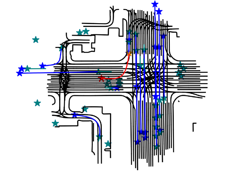
Figure 1: An example counterfactual collision from our framework generated by modifying a reference scenario from the Waymo Open Dataset Ettinger et al., (2021) with a perturbation derived from the MTR behavior model Shi et al., (2022). Our framework modifies the trajectory of an adversarial agent, using realistic behavior perturbations, to encourage a collision with a target agent along a reference trajectory. In this example, all reference trajectories are highlighted in blue, while the adversary’s trajectory is colored red. The non-adversarial agents’ initial and final positions are highlighted by a green and blue star, respectively; the adversary’s initial and final position are highlighted by a yellow and red star, respectively. We present a counterfactual in which the adversary performs an aggressive, over-wide right turn and collides with traffic stopped in the oncoming lane. Our approach offers valuable counterfactual scenarios – grounded in the notion of realism – on which to evaluate the maturity of existing AV collision avoidance technology.

For example, using an efficient and sufficient representation like Bird’s Eye View Liu and Niu, (2021), computer-generated scenarios and simulation-tested AV systems readily transfer learned safety behaviors to the real world in which case difficult scenario synthesis has the potential to increase AV robustness. This scenario generation and refinement must be automatic such that the generated features are more diverse and exhaustive as compared to manual generation.

Existing methods for generating adversarial scenarios face challenges in controlling realism and quality. While naive automated systems generate numerous scenarios, many are uninteresting. Therefore, selecting the most informative scenarios is crucial. We combine adversarial optimization with a learned behavior model quantifying scenario likelihood to respectively achieve critical and realistic scenario generation. Two key contributions are proposed:

1. Realistic Scenario Generation Framework: We present a general framework that optimizes perturbations to the weights of a pre-trained AV behavior model (which need only return a maximum a-posteriori output) to generate realistic counterfactual collision scenarios. We explicitly quantify the likelihood of the model’s parameterization, with respect to its training data, to enforce that any perturbations to a vehicle’s behavior are grounded in the realism captured by everyday interactions.

2. Representative Scenario Clustering for Testing: We cluster the synthetic counterfactual scenarios by diverse crash properties, e.g., crash angle and velocity, to reveal representative collision scenarios for downstream AV system testing. This counterfactual database offers a valuable test suite for developers, insurance companies and policymakers to evaluate the maturity and the risk of AV technology under diverse and realistic stress conditions.

We demonstrate our contributions on two state-of-the-art behavior prediction models and evaluate our counterfactual database on a baseline AV policy to produce interpretable failure modes.

II Related Work

AV Behavioral Models: Behavior modeling is crucial for AV systems, enabling the prediction of other traffic participants’ movements. Early works used simple dynamics models Kong et al., (2015) and rule-based simulators Dosovitskiy et al., (2017). Neural-network-based models have since demonstrated superior performance in predicting future movement Bansal et al., (2018); Cui et al., (2018). These models often employ a Bird’s Eye-View scene representation Cui et al., (2018); Varadarajan et al., (2021) and encode the map Shi et al., (2022) and the graph-interaction of participants Ivanovic and Pavone, (2018); Salzmann et al., (2020). While some models output multiple possible futures Cui et al., (2018); Varadarajan et al., (2021); Shi et al., (2022), others utilize a latent space approach for sampling Ivanovic and Pavone, (2018); Salzmann et al., (2020); Rempe et al., (2021). In this work, we desire a methodology to generate counterfactual scenarios that is compatible with all aforementioned architectures and is robust to future architecture development. Therefore, we only require the ability to evaluate a-posteriori likelihood from the behavior model, and are agnostic to specific input or internal representations.

Counterfactual Scenario Generation: Generating unsafe, critical scenarios often involves adversarial approaches, either gradient-free, e.g., evolutionary algorithms Biethahn and Nissen, (1997), or gradient-based Rempe et al., (2021, 2023); Cao et al., (2022). Some works utilize photo-realistic simulators Dosovitskiy et al., (2017) to generate plausible scenarios with 3D scene worlds O’Kelly et al., (2018), while many recent works focus on simpler scene representations. This work adopts a simpler approach and gradient-based optimization, unlike Wang et al., (2021); Vemprala and Kapoor, (2020); Klischat and Althoff, (2019), with the added constraint that the adversarial perturbations to behavior are grounded in the realism captured by a mature behavior model. Recent works have used generative models for scene construction Xu et al., (2023); Rempe et al., (2023); however, these works do not prioritize robust realism for the generated trajectory. Unlike these works, we offer a definition of realism through the lense of data-alignment in the model’s own parameter space.

Clustering-based Scenario Exposition: Representative scenarios, characterized by static factors, e.g., weather and road geometry, and dynamic factors, e.g., trajectories and velocities, reveal varying levels of risk across different behavioral models. Such scenarios are typically derived from databases rich in crash data, employing various clustering methods. These databases may include real-world data from crash reports Otte et al., (2003); Nitsche et al., (2017) or synthetic datasets designed for specific crash scenarios. Clustering techniques employed include KNN MacQueen et al., (1967); Lloyd, (1982), k-medoids Kaufman, (1990), hierarchical clustering Kaufman and Rousseeuw, (2009), density-based clustering Ester et al., (1996), and deep clustering methods Guo et al., (2017). In this work, we adopt the KNN technique to cluster synthetic counterfactual data by crash conditions, e.g., crash type and speed, for downstream AV safety evaluation. Therefore, our methodology offers a framework to reveal opportunities for further enhancements and areas in need of technological improvement within modern AV stacks.

Probabilistic Learned-Model Analysis: To develop a general likelihood quantification method for deep behavior models, we turn to the probabilistic analysis of deterministic, learned maximum a-posterior models. Unlike more experimental methods Kristiadi et al., (2020); Liu et al., (2021); E. Khan et al., (2019); Franchi et al., (2023), we utilize the general and model-agnostic Laplace approximation. While the Laplace approximation is generally intractable, efficient approximation methods exist Ritter et al., (2018); A. Daxberger et al., (2021). We opt for a sketching-based approach Tropp et al., (2016) which benefits from a strong theoretical analysis.

III Problem Formulation

III-A Problem Setup

In this work, we decompose driving scenarios into (i) a static scene description $S$ with semantic maps to identify the road and non-drivable area, e.g., road lanes, sidewalks, etc., (ii) the trajectories of $N$ non-adversarial vehicles $X=\{\textbf{X}^{i}\}_{i=1}^{N}$, sequences of 2D positions from a Bird’s Eye View, and (iii) the trajectory of the adversarial vehicle $\textbf{X}^{\text{adv}}$. Each trajectory $\textbf{X}^{i}=[x_{1}^{i},x_{2}^{i},\dots,x_{T}^{i}]^{\prime}\in\mathbb{R}^{T\times 2}\text{, where }T\in\mathbb{Z}_{+}$ is the final time, enumerates the state, $x_{t}^{i}$, for the $i$th agent at each time $t$; hence, $x^{\text{adv}}_{1}$ holds the initial condition for the adversarial agent. We assume access to a ground-truth trajectory for all non-adversarial agents in a real, reference scenario in which no collision occurs. The reference trajectory for all $N$ agents is given by $X_{\text{ref.}}=\{\textbf{X}^{i}_{\text{ref}}\}^{N}_{i=1}$. Further, we assume access to a learned behavior model $f_{\text{bhv.}}(\theta,x^{\text{adv}}_{1},X_{\text{ref.}},S)=\textbf{X}_{\text{bhv.}}^{\text{adv}}$, parameterized by a vector of model weights $\theta\in\mathbb{R}^{n}$, which jointly processes the adversary’s initial state, the reference trajectory of the $N$ non-adversarial agents and the scene description to produce a predicted trajectory for the adversary. Given these considerations, we desire a principled framework to choose the model weights $\theta$ such that the adversary’s predicted trajectory from $f_{\text{bhv.}}$ 1) creates a critical, unsafe scenario through a collision between itself and another agent and 2) is realistic. In particular, this work’s main contribution is the choice of model weights $\theta$ such that the adversary’s resultant trajectory is grounded in the notion of realism. Further, we seek a methodology to cluster these counterfactual scenarios according to similar descriptive features, e.g., velocity, thereby revealing the characteristics of the synthetic crashes to be used for safety evaluation.

III-B Objectives

The first objective is to synthetically generate realistic, counterfactual scenarios. Existing work on scenario generation, like Rempe et al., (2021), generates counterfactual scenarios by perturbing the behavior of existing scenarios. This process involves replacing the reference trajectory of an agent with the prediction from a behavior model such that we can adjust the model’s weights to cause a synthetic collision. We aim to extend this generation framework by viewing realism through the lense of an envelope of larger than a constant $c$ behavior probability density as defined by the behavior model itself. We visually depict such a condition in Figure 2.

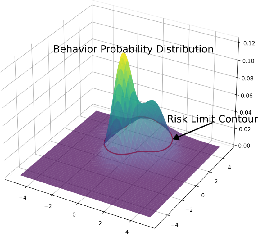
Figure 2: The risk contour $c$ offers a segmentation between realistic and unrealistic behavior with respect to a generic feed-forward behavior model.

As noted in Section II, the challenge in incorporating a variety of behavior model architectures into a generation framework is that each model may have a different output format: To remain compatible with as many models as possible, and to guard against future model development, we seek a methodology that only utilizes a model’s maximum a posteriori prediction to facilitate scenario generation.

With a counterfactual database, the second objective is identifying representative crash scenarios. We define representative scenarios by grouping crashes based on similarity and analyzing patterns within the resultant clusters, which involves three stages: (1) in crash reconstruction, the crashes are reconstructed using core features, such as velocities and angles, to represent the severity of the collision; (2) in clustering, the reconstructed crashes are clustered using an appropriate algorithm; and (3) in cluster analysis, the generated clusters are analyzed using descriptive features to expose the characteristics influencing vehicle response.

This process aims to identify representative scenarios, i.e., group synthetic counterfactuals by similar properties, which can then be used to evaluate AV stacks and provide insights for improvement. Feature selection and clustering algorithms should reflect meaningful clusters, i.e., a lower bound on the minimum cluster size, and consistent cluster representations, i.e., a high Silhouette score, in order to guide future development.

IV Approach

Our proposed technique acknowledges the challenge of objectively defining and measuring realism, particularly in complex driving scenarios. While achieving perfect realism might be elusive, existing behavior prediction models, trained on massive datasets, implicitly capture a high degree of realism through their ability to forecast real-world driving behavior accurately. This observation suggests a potential path: if the optimal model weights represent the peak of realism within the training data, then deviations from this point can be used to define a quantifiable region of realism. We focus on perturbing the weights of a behavior prediction model within a neigborhood of magnitude $r\in\mathbb{R}_{+}$, a hyperparameter in our algorithm, from the optimal point. By analyzing the scaled distance of the deviation from optimality in the parameter space, we can establish a measurable metric that captures scenarios deemed realistic within the context of the training data. This technique offers a valuable solution, swapping the subjective notion of realism for a measurable notion of “data-alignment," measured within the model’s parameter space.

In this section, we approximate the likelihood of a neural network’s parameterization, in a scalable manner, using the Laplace approximation and techniques from matrix sketching. We also provide considerations to guide weight selection such that the likelihood of the model is preserved and define the adversarial objective we use to incentivize a collision. Then, we state our main contribution by formulating the space of realistic model parameters as a constraint set for adversarial optimization. Finally, we detail the descriptive features by which we cluster the counterfactual database and present a second, parameter-efficient matrix sketching technique leveraging Low-Rank Adaptation.

IV-A Laplace Approximation

We employ the Laplace approximation to principally approximate the likelihood levels of any maximum a-posteriori model. We begin with a second-order expansion of the loss function, $\ell$, parameterized by a vector of weights $\theta\in\mathbb{R}^{n}$, e.g., a neural network, about optimality, $\theta^{\star}$,

$$\ell(\theta)\approx\ell(\theta^{\star})+\cancelto{0}{\nabla\ell(\theta^{\star})}^{T}\Delta\theta+\frac{1}{2}{\Delta\theta}^{T}H(\theta^{\star})\Delta\theta,$$ (1)

where $\Delta\theta=\theta-\theta^{\star}\in\mathbb{R}^{n}$ is a parameter perturbation from optimality.

Further, suppose that we define the loss function to correspond to the negative log posterior on the underlying weight distribution such that

$$\ell(\theta)=-\log p\left(\theta\mid\mathcal{D}\right)\approx-\log p\left(\theta^{\star}\mid\mathcal{D}\right)+\frac{1}{2}{\Delta\theta}^{T}H\Delta\theta,$$ (2)

which leads to the interpretation of a Gaussian belief distribution over $\theta$, i.e.,

$$\theta\sim\mathcal{N}\left(\theta^{\star},H^{-1}\right)~{}~{}~{}~{}~{}~{}\text{with}~{}~{}\Sigma=H^{-1}.$$ (3)

However, the Hessian inverse covariance is computationally intractable as it exists in $\mathbb{R}^{n\times n}$ and $n$, the number of model parameters, is typically very large for deep learning models. Therefore, for likelihood estimation, we require an accurate and computationally efficient technique in order to develop an approximation of the Hessian inverse covariance.

IV-B Symmetric Matrix Sketching

We turn to numerical sketching to tractably approximate the Hessian’s most important covariance components, which allows us to compress the top energy components of the Hessian efficiently. Matrix sketching is a technique that allows one to approximate a dense matrix $H$ as a product of low-rank factors, typically, $AQ$ where $A\in\mathbb{R}^{n\times k}$, $Q\in\mathbb{R}^{k\times n}$ and $k\ll n$. Alternatively, if $H$ is symmetric, we can use the 3-factor low-rank approximation $UDU^{T}$ where $U\in\mathbb{R}^{n\times k}$ and $D\in\mathbb{R}^{k\times k}$. Randomized sketching, an efficient sketching algorithm, is known to converge to a low-rank approximation of the top-energy components of the matrix $H$ Tropp et al., (2016). Therefore, we can use such an algorithm to quantify the directions in the parameter space that lead to the fastest decrease in the likelihood. We reproduce an efficient sketching algorithm from Tropp et al., (2016) in the Appendix Section VII-B.

IV-C Minimizing Probability Loss when Choosing $\Delta z$

After establishing an estimate of the Hessian inverse covariance, we desire guidelines to reveal the weight perturbations, $\Delta\theta\in\mathbb{R}^{n}$, that result in a minimal decrease to the likelihood of the model’s weights. Our objective is to develop a fixed-rank projection of an arbitrary vector $z\in\mathbb{R}^{|z|}$ defined as

$$\tilde{\Delta z}=(I-PP^{T})\Delta z,$$ (4)

such that $\tilde{\Delta z}^{T}H\tilde{\Delta z}$ is minimized. We formulate this objective as

$$\operatorname{minimize}_{P} ~{}~{}~{}~{}{\Delta z}^{T}(I-PP^{T})^{T}H(I-PP^{T})\Delta z$$ (5)

$$\operatorname{such~{}that} ~{}~{}~{}~{}P^{T}P=I\text{ and }\forall\Delta z\in\mathbb{R}^{|z|}.$$

Then, this objective can be reformulated as

$$\operatorname{minimize}_{P} ~{}~{}~{}~{}\left|\left|H(I-PP^{T})\right|\right|_{\text{op}}$$ (6)

$$\operatorname{such~{}that} ~{}~{}~{}~{}P^{T}P=I,$$

whose solution, for a fixed rank $k$, is to remove components from $z$ which correspond to the highest singular values in $H$, i.e.,

$$P^{\star}=U[:,1:k]~{}~{}~{}\text{where}~{}~{}~{}USU^{T}=H.$$

Projection Operation: In linear algebra, a projection of the vector z $\in\mathbb{R}^{n}$ onto the range of a square matrix $A\in\mathbb{R}^{n\times n}$ produces the vector $\hat{z}\in\mathbb{R}^{n}$ given by

$$\hat{z}=A(A^{T}A)^{-1}A^{T}z.$$

For an orthonormal matrix $P$, satisfying $P^{T}P=I$, this projection operation gives $\hat{z}$ as

$$\hat{z}=P(\cancelto{I}{P^{T}P})^{-1}P^{T}z.$$

Therefore, we can write the complementary rejection of directions as

$$\tilde{z}=z-\hat{z}=z-PP^{T}z=(I-PP^{T})z,$$

in which case the operation $(I-PP^{T})$ removes the components of $z$ in the range of $P$.

IV-D Adversarial, Collision-inducing Objective

In order to incentivize a collision between two vehicles in the environment, we formulate an adversarial objective for the adversary in the scenario. From the problem formulation, we assume we have access to a behavior model $f_{\text{bhv.}}$, parameterized by weights $\theta\in\mathbb{R}^{n}$, in order to predict the adversary’s state trajectory. We construct a simple collision loss with these primitives, akin to the formulation in Rempe et al., (2021), by choosing $\theta$ to minimize the minimum separation over time of the distance between the adversarial vehicle, $\textbf{X}^{\text{adv}}$, and each targeted neighbor, $\textbf{X}^{\text{target}}_{\text{ref.}},$ in the optimization batch with the added constraint that we restrict the search space of $\theta$ to the set of realistic model parameters, $\mathcal{C}_{\text{realism}}$:

$$\operatorname{minimize}_{\theta}{}{}{} f_{0}(\theta):=\operatorname{softmin}_{T}\left|\left|{\textbf{X}^{\text{adv}}-\textbf{X}^{\text{target}}_{\text{ref.}}}\right|\right|_{2}$$ (7)

$$\operatorname{such~{}that}{}{}{} \textbf{X}^{\text{adv}}:=f_{\text{bhv.}}(\theta,\textbf{X}_{1}^{\text{adv}},X_{\text{ref.}},S)\in\mathbb{R}^{T\times 2},$$

$$S\equiv\text{scene description},$$

$$\theta\in\mathcal{C}_{\text{realism}}.$$

IV-E Optimization with Projection Feasibility Constraint

Finally, we offer a definition for the space of realistic model parameters as a constraint set for the aforementioned adversarial objective, $f_{0}$. We turn to the projected gradient descent method in the presence of constraints. For the minimization of an adversarial loss $f_{0}$ over the domain of a model’s parameters, $\theta\in\mathbb{R}^{n}$, we ensure realism by 1) confining $\theta$ to a neighborhood about $\theta^{\star}$, the pretrained optimum, of magnitude the hyperparameter $r\in\mathbb{R}_{+}$ using the L2 norm and 2) enforcing that weight perturbations must be orthogonal to the range of $P$ spanned by the directions leading to fastest decrease in the likelihood of the model; hence, weight perturbations used in the minimization of $f_{0}$ preserve likely behavior from the perspective of the behavior model:

$$\operatorname{minimize}_{\theta}{}{}{} f_{0}(\theta)$$ (8)

$$\operatorname{such~{}that}{}{}{} \mathcal{C}_{\text{realism}}:=\begin{cases}\left|\left|{\Delta\theta}\right|\right|_{2}=\left|\left|{\theta-\theta^{\star}}\right|\right|_{2}\leq r\\ PP^{T}\Delta\theta=PP^{T}\left(\theta-\theta^{\star}\right)=0\end{cases}.$$

Given this formulation above, the constraints projections are provided as

$$\Pi_{P}(\theta)=\operatorname{argmin}_{PP^{T}(\tilde{\theta}-\theta^{\star})=0}\left|\left|{\tilde{\theta}-\theta}\right|\right|_{2}^{2}=\theta-PP^{T}(\theta-\theta^{\star}),$$

and

$$\Pi_{\left|\left|{\Delta\theta}\right|\right|\leq r} =\begin{cases}\theta~{}~{}\text{if}~{}~{}\left|\left|{\theta-\theta^{\star}}\right|\right|_{2}^{2}\leq r,\\ \theta^{\star}+\frac{r}{\left|\left|{\theta-\theta^{\star}}\right|\right|_{2}^{2}}(\theta-\theta^{\star})~{}~{}\text{otherwise}\end{cases}.$$ (9)

IV-F Clustering-based Representative Critical Scenarios

After generating a counterfactual database, we aim to identify representative collision scenarios for testing autonomy stacks. We group similar crashes using clustering to extract these cases.

We focus on core features related to vehicle dynamics before the crash, reflecting our key concerns about crashes. These features include velocity, relative velocity, and angle of impact. Additionally, we include features signifying the tested vehicle’s response, such as response time. We categorize the angle feature into crash type, e.g., contrasting, side-left, side-right and chasing. We define a "contrasting" crash to occer when the adversary is in the oncoming lane, while a "side-left", or "side-right", crash to occur with the adversary to the left, or right, of the target; we define a "chasing" crash to occur when the adversary begins trailing the target.

For descriptive features, we use: Adversarial vehicle speed $v_{\text{a}}$; Longitudinal relative speed $\Delta v_{x}$; Lateral relative speed $\Delta v_{y}$; Angle of impact $\gamma$; Crash type $\beta$; and response time $t_{r}$. Table II in the Appendix Section VII-F gives detailed descriptions of these features.

We use K-Nearest Neighbors (KNN) for clustering and evaluate the quality of the chosen clusters using the average Silhouette score Shahapure and Nicholas, (2020). We impose a constraint on the smallest cluster size to prevent the formation of non-representative clusters. The choice of this size is dataset-specific and is discussed in the results section.

IV-G Low-Rank Adaptation in Efficient Sketching

Also, we propose an alternative to sketching the full Hessian inverse covariance: we sketch the Hessian in a lower dimensional, parameter-efficient space with Low-Rank Adaptation. For every NN layer representable as a matrix $W$, Low-Rank Adaptation enables parameter-efficient perturbations to the layer’s weight space by adding a low-rank additive factor, i.e.,

$$\tilde{W}=W+AB,$$

where $A\in\mathbb{R}^{m\times k}$ and $B\in\mathbb{R}^{k\times n}$. For $k\ll\{m,n\}$ and, importantly, at initialization,

$$A_{ij}\sim\mathcal{N}(0,\sigma)~{}~{}~{}~{}B_{kl}=0.$$

In this approach, we sketch merely the factors $A$ and $B$ at their initialization point. In the Appendix Section VII-C, we investigate the convergence of the Global Information Projection Matrix, which is the ability to extract the most energetic directions in the parameter space from the Laplace approximation for each sketching approach.

V Results

In this section, we encapsulate the descriptive features from our synthetic counterfactual database by forming diverse, representative crash clusters, and we evaluate the response of a baseline AV policy on this dataset to expose the policy’s strengths and weaknesses.

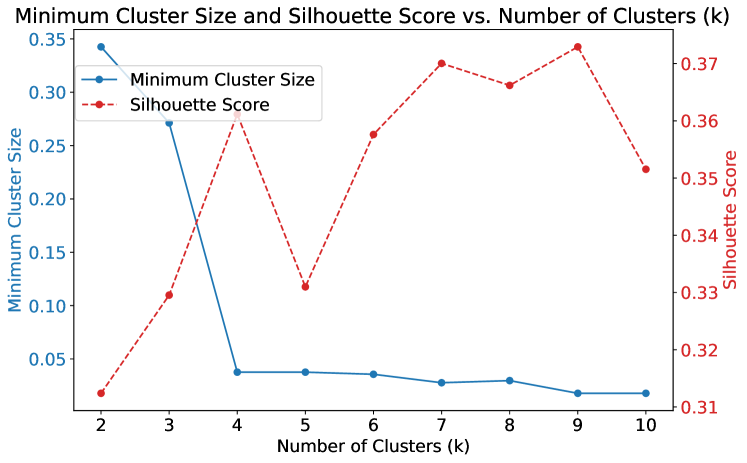
Figure 3: The number of clusters balances a representative set of scenarios, measured through the minimum cluster size, and the effectiveness of the clustering algorithm, measured by the Silhouette score. $k$, the number of clusters, achieves a low minimum cluster size and high Silhouette score for $k=8$.

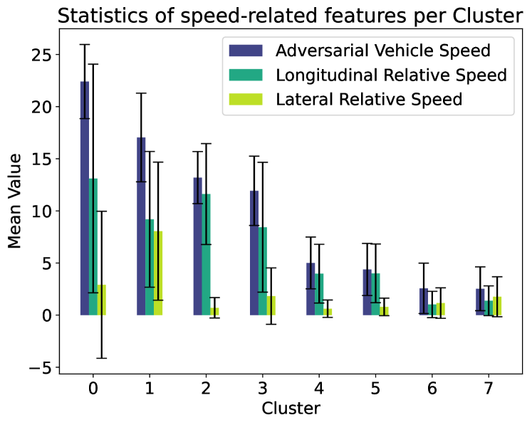
Figure 4: Clusters are numbered in descending order with respect to the severity of the collision by virtue of the mean adversarial vehicle speed.

Our proposed counterfactual generation pipeline is agnostic to the underlying behavior model. We, therefore, use two distinct behavioral models: MTR and Trajectron++ Shi et al., (2022); Salzmann et al., (2020). As discussed in Section VI-B, we only present our findings for one representative behavioral model, i.e., MTR, in the main body. We evaluate the response of a baseline AV policy on the target, non-adversarial vehicle with limited reactivity in each counterfactual. The policy monitors the position and velocity of all agents, predicts the time and minimum distance to collision, assuming constant velocity extrapolation, and chooses to emergency brake if either measure is below a prescribed value; otherwise, the policy follows the reference trajectory using a single-step Model Predictive Control, obeying acceleration limits. The exact implementation of the baseline policy is provided in the Appendix Section VII-D.

For the MTR behavior model, the collisions are generated with a prescribed realism hyperparameter $r=0.003$ whose value is determined as discussed in Section VI-A. The generated counterfactual dataset comprises a total of 505 collisions. We have set a threshold for the smallest cluster size at 3% of the total dataset, aiming to identify clusters of relevant and representative scenarios. Therefore, we chose $k=8$ clusters in this case as shown in Figure 3. Final detailed statistics of the clusters are presented in Table I. The clusters are labeled in descending order of the adversarial vehicle speed, $v_{a}$, from more intense to less intense testing conditions, i.e., see Figure 4.

Descriptive Feature	Cluster 0	Cluster 1	Cluster 2	Cluster 3	Cluster 4	Cluster 5	Cluster 6	Cluster 7
Adversarial Vehicle Speed $v_{a}$	22 (3.5)	17 (4.2)	13 (2.5)	12 (3.3)	5.0 (2.5)	4.4 (2.5)	2.6 (2.4)	2.5 (2.1)
Longitudinal Relative Speed $\Delta v_{x}$	13 (11)	9.2 (6.5)	12 (4.8)	8.4 (6.2)	4.0 (2.8)	4.0 (2.8)	1.0 (1.3)	1.4 (1.4)
Lateral Relative Speed $\Delta v_{y}$	2.9 (7.1)	8.1 (6.6)	0.70 (0.98)	1.8 (2.7)	0.61 (0.83)	0.79 (0.84)	1.2 (1.5)	1.8 (1.9)
Crash Type $\beta$
Chasing	12 [43%]	4 [27%]	91 [100%]	0	120 [98%]	0	0	14 [17%]
Contrasting	7 [25%]	3 [20%]	0	51 [91%]	0	67 [100%]	10 [23%]	0
Side-left	4 [14%]	7 [47%]	0	1 [2%]	3 [2%]	0	34 [77%]	0
Side-right	5 [18%]	1 [7%]	0	4 [7%]	0	0	0	69 [83%]
Tested Vehicle Response
No response	0	0	0	0	9 [7%]	12 [18%]	26 [59%]	46 [55%]
Response	28 [100%]	15 [100%]	91 [100%]	56 [100%]	112 [93%]	55 [82%]	18 [41%]	37 [45%]
Response Time $t_{r}$	6.7 (1.4)	7.2 (0.68)	5.2 (1.5)	6.1 (1.8)	5.0 (1.9)	5.6 (1.7)	6.0 (2.4)	2.8 (2.6)

TABLE I: Synthetic counterfactuals are clustered according to descriptive crash properties. We find that the baseline policy responds best to high-speed collisions and struggles to detect "side-left" and "side-right" crash types at low speeds.

These diverse clusters reveal distinct patterns in the behavior of tested vehicles under various crash scenarios, providing insights into the operational challenges and efficiencies of a candidate AV policy.

High-Speed Clusters: Clusters 0 and 1, characterized by high testing speeds, i.e., 22.41 m/s and 13.19 m/s, respectively, predominantly feature "chasing" and "side-left" crashes. We assume the tested vehicle to have produced a "response" if the target correctly reacts to an imminent collision with the adversary by beginning to brake. Therefore, the 100% response rate in both clusters 0 and 1 suggests the effective handling of high-stress conditions, indicating advanced detection and robust response from the baseline policy.

Mid-Speed Clusters: Clusters 2 and 3 demonstrate a lower mean testing speed, i.e., 13.19 m/s and 11.92 m/s, respectively, with a dominant number of "chasing" and "contrasting" crashes. We define a "contrasting" crash to occur when the adversary is in the oncoming lane. The 100% response rate in both clusters highlights the system’s effectiveness in detecting and reacting to both tailing and oncoming vehicle collisions.

Low-Speed, High Complexity Clusters: Cluster 4 showcases an almost complete response rate of 93% despite a lower testing speed of 5.01 m/s, indicating high vigilance from the AV policy in tracking vehicles from behind at slower speeds. Cluster 5 reveals challenges in less predictable crash scenarios with an 18% no-response rate to "contrasting" crashes, suggesting potential shortcomings in head-on detection at low speeds.

The Most Challenging Clusters: Clusters 6 and 7, with the lowest testing speeds, are dominated by "side-left" and "side-right" crashes, respectively, both presenting high no-response rates at 59% and 55% as shown in Table I. This poor response rate may indicate difficulties for the policy to detect and react to lateral threats at low speeds, highlighting a potential weaknesses in the baseline’s limited reactivity.

We offer Table I to present a holistic view of our counterfactual database; however, any one counterfactual is only valuable to the extent the scenario is realistic. The patterns across clusters highlight that these counterfactuals demonstrate diverse crash characteristics, e.g., a variety in crash severity and crash type, which, more importantly, are also grounded in the notion of realism by virtue of the realistic behavior captured by the pre-trained behavior model. Therefore, this counterfactual generation pipeline offers the opportunity for critical insights to strengthen AV technology with a broad spectrum of real-world scenarios. For example, severe crashes with high response rates present opportunities for continued improvement, while less severe instances, with relatively high no-response rates, offer critical areas in need of technological improvements, particularly in sensor accuracy and response algorithms for the baseline policy.

VI Discussion

VI-A The choice of $r$

The realism radius $r$ is a hyperparameter trading off fidelity to the most data-aligned, i.e, “realistic", prediction and aggressiveness of the desired behavior. One cannot prescribe a single value $r$ that would work in all cases, but we make two observations: 1) by expressing $r$ as a constraint rather than a soft objective, it is not affected by scaling the adversarial objective function; and 2) because $r$ is always a scalar, we can use conformal prediction Shafer and Vovk, (2008); Angelopoulos et al., (2023) to determine its value in practice with a small calibration set. In our experiments, we set $r$ using the bisection method until each scenario contains a non-severe collision by visually inspecting the resultant behaviors on a small ($n=10$) calibration set.

VI-B Selection of behavioral models

We highlight that our method is versatile and applicable to any parametric behavioral model. We demonstrate our pipeline on two representative behavior models: a regressive model Salzmann et al., (2020) and a transformer-based model Shi et al., (2022). We have detailed the results for the transformer-based model Shi et al., (2022) in the paper’s main body, while, for brevity, we present the findings for the regressive model Salzmann et al., (2020) in the Appendix Section VII-G with discussion. Further, we visually depict a synthetic counterfactual collision from each behavior model in Figure 1, on the main body’s first page, and in Figure 8 in the Appendix Section VII-E.

VII Conclusions

This work proposes a novel framework for generating realistic and challenging scenarios for AV testing using limited collision-free data. The approach combines adversarial optimization with a trained behavior model, enabling the quantification of scenario likelihood and ensuring the generation of realistic counterfactual scenarios. Our framework leverages the Laplace approximation and sketching techniques for computationally scalable likelihood estimation, overcoming the limitation of previous work. The method is agnostic to the underlying behavior model or adversarial loss and is scalable, making it a versatile tool for testing AV systems in unsafe situations with a collision. We show a scaling-friendly parametrization based on the Low-Rank Adaptation reformulation. We demonstrate the effectiveness of our work on two state-of-the-art behavior prediction models and two distinct driving datasets. Furthermore, we identify representative and diverse crash conditions among the synthetic data based on KNN clustering for downstream policy evaluation. Our framework offers a systematic approach to generate realistic counterfactual collisions with various AV behavior models; therefore, our approach offers diverse, high-fidelity and simulated stress conditions to reveal the strengthes and weaknesses of AV technologies for AV stakeholders, e.g., car manufacturers, insurance companies and government regulators.

APPENDIX

VII-A LoRA Hessian Computation

We observe that despite reducing the required memory and computation by taking only the top eigenvector components of the inverse covariance matrix, $P\in\mathbb{R}^{n\times k}$, the representation can still be too large, some large ML models fit in memory only once, implying $k=1$. and only one eigenvector component can be used.

Instead, we turn to another compressed representation of the NN parameter representation. Importantly, this is not a third approximation in our algorithm: we perform the Laplace approximation in a smaller parameter space. Many choices exist for a reduced parameter space, the most obvious being a subset of network parameters. However, inspired by recent advances in fine-tuning large language models, we reparametrize the network using the Low-Rank Adaptation parameter space Hu et al., (2021).

Since $P$ is constructed, we can use a network reparametrization before constructing the Laplace approximation, i.e.,

$$\forall W_{i}~{}~{}~{}~{}\text{let}~{}~{}~{}~{}\widetilde{W}_{i}=W_{i}+B_{i}A_{i},$$

where $B_{i}=0$ and $A_{i}\sim\mathcal{N}(0,\sigma I)$.

For a new parametrization, for the Laplace approximation, we need $\nabla_{p}\ell=0$ and $\nabla_{p}^{2}\ell\neq 0$. Therefore, because

$$\nabla_{\{A,B\}}\ell(W_{i}+BA)=\left(\nabla_{\widetilde{W}_{i}}\ell(\widetilde{W}_{i})\right)\{B,A^{T}\},$$

and at trained network optimality $\nabla_{\widetilde{W}_{i}}\ell(\widetilde{W}_{i})=0$, then $\nabla_{p}\ell=0$ and

$$\nabla_{A}^{2}\ell=(I\otimes B)HB=0,$$

$$\nabla_{B}^{2}\ell=(I\otimes A^{T})HA^{T}\neq 0.$$

Hence, we retain only $B_{i}$ parameters for the new parametrization.

VII-B Sketching

Below, in Algorithms 1, 2 and 3 we reproduce an efficient random sketching algorithms from Tropp et al., (2016). While Tropp et al., (2016) offers several possible random sketching algorithms, we focus on the symmetric positive decomposition consisting of 2 factors

$$H\approx USU^{T}.$$

We specifically retrieve the positive semi-definite factor $S$ given that under Laplace method Gaussian approximation, the Hessian, or the inverse covariance matrix is positive semi-definite.

VII-B1 Hessian matrix spectral decay in sketched matrices in Salzmann et al., (2020); Shi et al., (2022)

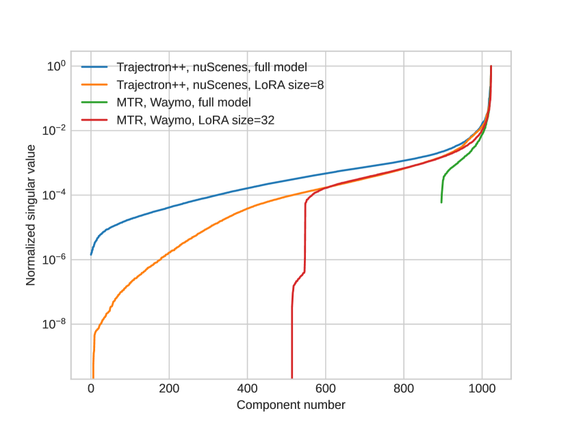
Figure 5: Singular values of the sketching decomposition of the Hessian matrix for the Trajectron++ and MTR models Salzmann et al., (2020)Shi et al., (2022). Rapid decay of singular values indicates that a low-rank approximation captures most of the singular-value energy within the matrix.

VII-B2 Sketching algorithms applied in this work

Below, we concisely reproduce the sketching algorithms exploited in this work for sketching positive definite matrices comprising the covariance in the Laplace method as applied to the behavior model’s parameter space. The sketching matrices are obtained as the result of Algorithm 3, but Algorithms 1 and 2 are called as subroutines.

1:Left sketch matrix $\Psi$, Right sketch matrix $\Phi$

2:Left sketch $W=\Psi A$, Right sketch $Y=A\Phi$

3:function low_rank($\Psi$, $\Phi$, $W$, $Y$)

4:     $Q,\_\leftarrow\operatorname{\tt{qr}}(Y)$ $\triangleright$ left orthonormal basis

5:     $U,T\leftarrow\operatorname{\tt{qr}}(\Phi Q)$

6:     $X\leftarrow T^{{\dagger}}\left(U^{*}W\right)$ $\triangleright$ triangular solve

7:     return $Q$, $X$ $\triangleright$ $A\approx QX$

8:end function

Algorithm 1 Sketching Algorithms Reproduced From Tropp et al., (2016)

1:Left sketch matrix $\Psi$, Right sketch matrix $\Phi$

2:Left sketch $W=\Psi A$, Right sketch $Y=A\Phi$

3:function low_rank_sym($\Psi$, $\Phi$, $W$, $Y$)

4:     $Q,X\leftarrow{\tt low\_rank}(\Psi,\Phi,W,Y)$

5:     $U,T\leftarrow\operatorname{\tt{qr}}([Q,X^{*}])$ $\triangleright$ orthogonalize concatenation

6:     $T1\leftarrow T[:,1:k]$ and $T2\leftarrow T[:,k+1:2k]$ $\triangleright$ split

7:     $S\leftarrow(T_{1}T_{2}^{*}+T_{2}T_{1}^{*})/2$ $\triangleright$ symmetrize

8:     return $U,S$ $\triangleright$ $A\approx USU^{*}$

9:end function

Algorithm 2 Sketching Algorithms Reproduced From Tropp et al., (2016)

1:Left sketch matrix $\Psi$, Right sketch matrix $\Phi$

2:Left sketch $W=\Psi A$, Right sketch $Y=A\Phi$

3:function low_rank_psd($\Psi$, $\Phi$, $W$, $Y$)

4:     $U,S\leftarrow{\tt low\_rank\_sym}(\Psi,\Phi,W,Y)$

5:     $V,D\leftarrow\operatorname{\tt{eig}}(S)$ $\triangleright$ eigendecomposition

6:     $U\leftarrow UV$ $\triangleright$ consolidate orthonormal factors

7:     $D\leftarrow\max(D,0)$ $\triangleright$ remove negative eigenvalues

8:     return U, D $\triangleright$ $A\approx UDU^{*}$

9:end function

Algorithm 3 Sketching Algorithms Reproduced From Tropp et al., (2016)

VII-C Convergence of Global Information Estimate

We investigate the convergence of the Global Information Projection Matrix, which is the ability to extract the most energetic directions in the parameter space from the Laplace approximation. In Figure 6, we show that the Hessian converges rapidly – at 10% of the dataset, the number of captured linear directions is above 80%.

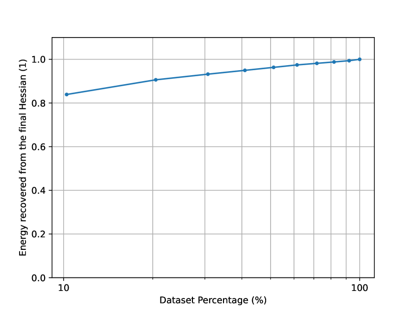
Figure 6: Global Information Projection (GIP) Matrix converges quickly for a fixed rank size $k$ with the number of scenarios in the training dataset.

Likewise, for the Low-Rank Adaptation sketching case, we observe similar but more rapid convergence to the final extracted linear subspace in Figure 7 presented in the Appendix. We theorize this is due to the inherently smaller parameter space through the use of Low-Rank Adaptation. The fast convergence in Figure 6 and Figure 7 justifies that our fixed rank approximation of the Hessian only requires a fraction of the dataset; therefore, our proposed approach can be extended to large-scale behavior models trained on prohibitively large datasets.

Additionally, we quantify the decay of the singular values in the symmetric positive-definite sketching decomposition of the Hessian matrix in Figure 5 and observe, like other works, e.g., Sharma et al., (2021), that the singular values of deep learned models decay rapidly. This result suggests that the sketching decomposition is an excellent approximation of the Hessian matrix.

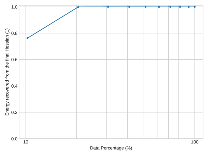
Figure 7: LoRA case: GIP matrix converges quickly for a fixed rank size $k$ with the number of scenarios in the training dataset.

VII-D Baseline AV Policy For Evaluation

The baseline policy used in this work for modeling the reaction of other agents needed to be (i) adhering as closely to a reference trajectory (e.g., recorded behavior in the scene) but also (ii) reasonably realistic, allowing for an agent to react to the adversarial behavior directed at it. The policy monitors the position and velocity of all agents, predicts the time and minimum distance to collision assuming constant velocity extrapolation, and chooses to emergency brake if either measure is below a prescribed value; Otherwise, the policy follows the reference trajectory using a single-step Model Predictive Control, obeying acceleration limits.

The mathematical formulation takes the form

$$\min_{a(t)}\quad ||x(t+1)-x_{ref}(t+1)||^{2}$$

$$~{}~{}~{}~{}~{}~{}~{}+\frac{1}{10}||v(t+1)-v_{ref}(t+1)||^{2}$$

s.t. $$x(t+1)=x(t)+v(t)\Delta t,$$

$$v(t+1)=v(t)+a(t)\Delta t,$$

$$d(x(t+1),x_{i}(t+1))\geq d_{min},$$

$$t_{coll.}(x(t+1),v(t+1),x_{i}(t+1),v_{i}(t+1))\geq t_{min},$$

$$-a_{max}\leq a(t)\leq a_{max},$$

VII-E Collision Examples

Examples of generated collisions are presented in the main body with Figure 1 and in the Appendix with Figure 8.

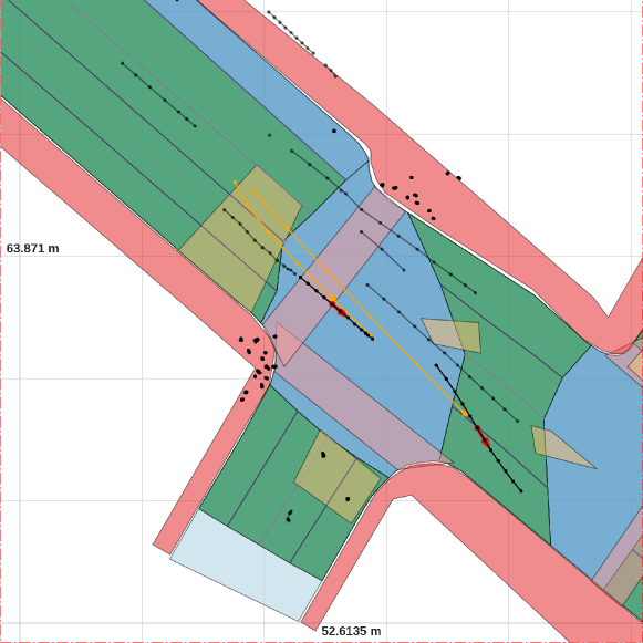
Figure 8: Example of generated collisions with other traffic participants using the nuScenes dataset and the Trajectron++ behavior model. The aggressive agent collides with the vehicle in the neighboring lane.

Features	Type	Description
Adversarial vehicle speed $v_{\text{a}}$	Numeric	The magnitude of velocity for the adversarial vehicle right before the crash.
Longitudinal relative speed $\Delta v_{x}$	Numeric	The maginitude of the relative velocity of the two crashing parties right before the crash in the longitudinal direction of the tested vehicle.
Lateral relative speed $\Delta v_{y}$	Numeric	The magnitude of the relative velocity of the two crashing parties right before the crash in the lateral direction of the tested vehicle.
Angle of impact $\gamma$	Numeric	The relative angle of two crashing parties at the crash.
Crash type $\beta$	Categorical	Types of crashes categorized by the angle of impact. Types include contrasting, chasing, side-left and side-right.
Response time $t_{r}$	Numeric	The time, in seconds, before the tested vehicle responds, i.e., brakes, to the crash, if there is a response.

TABLE II: Core and descriptive features for generated collision clustering analysis.

VII-F Quantifiable dynamics features used for behavioral clustering

Our clustering analysis focuses on identifying representative critical scenarios for testing autonomous vehicle stacks by grouping similar crashes. To achieve this, we employ a combination of core and descriptive features. The core features, which reflect key concerns about crashes, include velocity, relative velocity, and angle of impact. Additionally, the response time of the tested vehicle is considered a core feature.

Descriptive features, on the other hand, categorize the angle feature into distinct crash types (contrasting, side-left, side-right, chasing). These features, along with the core features, are then used for clustering. The study utilizes the K-Nearest Neighbors (KNN) algorithm for clustering, ensuring representativeness by imposing a constraint on the smallest cluster size to prevent the formation of non-representative clusters.

The detailed description of the features are contained in Table II.

VII-G Representative Critical Scenarios for Salzmann et al., (2020)

In this section, we present our findings based on an exemplary behavioral model Salzmann et al., (2020). The collisions are generated with a prescribed realism parameter $r=0.03$. The dataset comprises a total of 174 collisions. We have set a threshold for the smallest cluster size at 5% of the total dataset, aiming to identify a concise set of representative scenarios. For our analysis, we chose $k=5$, illustrated in Figure 9.

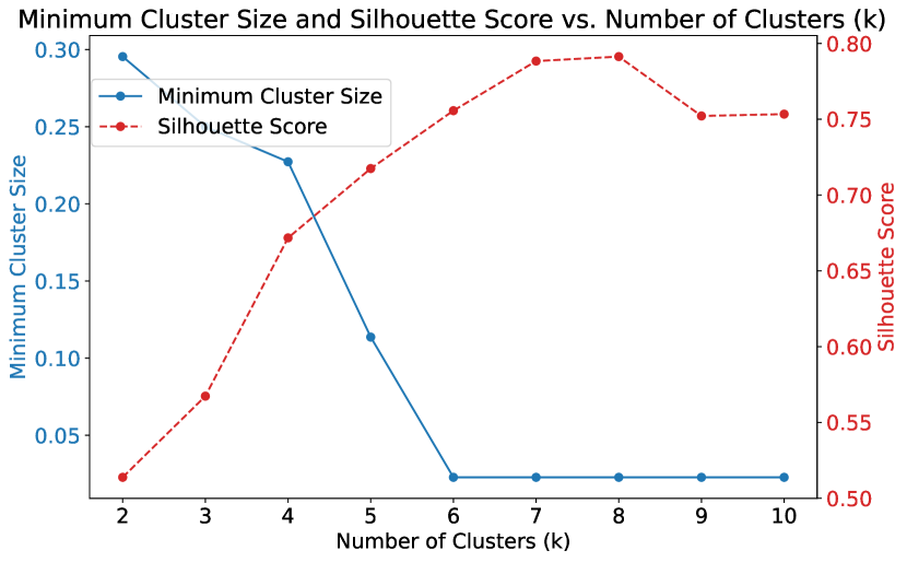
Figure 9: Choice of $k$: a balance of Silhouette Score and minimum cluster size.

As illustrated in Figure 11, Cluster 1, with relatively higher testing speed, demonstrates an exceptional response rate, with "Chasing" crashes constituting 90% and "Side-left" crashes 10%. The complete response rate in this cluster highlights its advanced detection capabilities, showcasing robust performance even under challenging conditions.

In contrast, the other clusters display varying levels of non-responsiveness, each highlighting different challenges in vehicle response systems. Cluster 0: Characterized by the highest testing speed, this cluster exclusively involves "Chasing" crashes (100%), typically indicating high-speed rear-end collisions. Despite these demanding conditions, the response rate of 67% reflects that the vehicle systems are generally well-equipped to manage such high-stress scenarios. Cluster 2: With a lower testing speed of 5.80 m/s, this cluster predominantly experiences "Chasing" (90%) and "Side-left" (10%) crashes. The notably high no-response rate (90%) underlines possible inadequacies in the vehicle’s sensor accuracy or algorithmic agility, especially in less severe but complex rear-following collisions. Comparing Cluster 0,1,2 together, a deeper investigation into the chasing type collisions is necessary to find out potential system deficiencies.

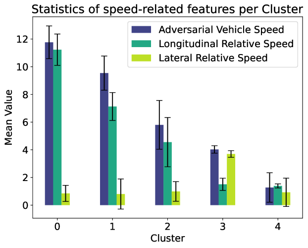
Figure 10: Comparison of clusters via speed-related features.

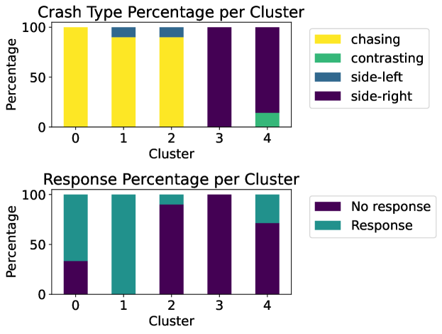
Figure 11: Comparison of angle and response characteristics across resultant scenario clusters.

Cluster 4, characterized by a low testing speed, predominantly involves "Side-right" crashes (86%) and has a low response rate of 29%. Cluster 3 exhibits a complete lack of response, with all incidents being "Side-right" crashes at a low speed. These high non-responsiveness rates severely underscore the challenges in detecting lateral threats from the right, pinpointing a critical need for improvements in low-speed collision detection technologies.

Overall, while Cluster 1 sets a benchmark with its full responsiveness, the varied performance across other clusters emphasizes the need for enhanced sensor capabilities and refined algorithms. This disparity particularly necessitates further research into improving detection and response mechanisms in scenarios that currently exhibit high rates of non-responsiveness.

Descriptive Feature	Cluster 0	Cluster 1	Cluster 2	Cluster 3	Cluster 4
Adversarial Vehicle Speed $v_{a}$
Mean	11.765	9.541	5.800	4.025	1.275
Std	1.183	1.234	1.761	0.270	1.063
Longitudinal Relative Speed $\Delta v_{x}$
Mean	11.233	7.126	4.551	1.505	1.388
Std	1.132	1.007	1.779	0.442	0.147
Lateral Relative Speed $\Delta v_{y}$
Mean	0.847	0.804	0.989	3.696	0.927
Std	0.582	1.088	0.709	0.241	1.023
Crash Type $\beta$
Chasing	48 (100%)	36 (90%)	36 (90%)	0	0
Contrasting	0	0	0	0	4 (14%)
Side-left	0	4 (10%)	4 (10%)	0	0
Side-right	0	0	0	20 (100%)	24 (86%)
Tested Vehicle Response
No response	16 (33%)	0	36 (90%)	20 (100%)	20 (71%)
Response	32 (67%)	40 (100%)	4 (10%)	0	8 (29%)

TABLE III: Clustering results for the generation based on the behavioral model in Salzmann et al., (2020).

References

- A. Daxberger et al., (2021) A. Daxberger, E., Kristiadi, A., Immer, A., Eschenhagen, R., Bauer, M., and Hennig, P. (2021). Laplace Redux - Effortless Bayesian Deep Learning. Neural Information Processing Systems.
- Abeysirigoonawardena et al., (2019) Abeysirigoonawardena, Y., Shkurti, F., and Dudek, G. (2019). Generating Adversarial Driving Scenarios in High-Fidelity Simulators. In IEEE International Conference on Robotics and Automation.
- Alireza Samerei et al., (2021) Alireza Samerei, S., Aghabayk, K., Shiwakoti, N., and Mohammadi, A. (2021). Using latent class clustering and binary logistic regression to model Australian cyclist injury severity in motor vehicle-bicycle crashes. Journal of Safety Research.
- Angelopoulos et al., (2023) Angelopoulos, A. N., Bates, S., et al. (2023). Conformal prediction: A gentle introduction. Foundations and Trends® in Machine Learning, 16(4):494–591.
- Bansal et al., (2018) Bansal, M., Krizhevsky, A., and Ogale, A. (2018). ChauffeurNet: Learning to Drive by Imitating the Best and Synthesizing the Worst. Robotics: Science and Systems.
- Biethahn and Nissen, (1997) Biethahn, J. and Nissen, V. (1997). Evolutionary algorithms in management applications. Journal of the Operational Research Society, 48(3):333–334.
- Cao et al., (2022) Cao, Y., Xiao, C., Anandkumar, A., Xu, D., and Pavone, M. (2022). AdvDO: Realistic Adversarial Attacks for Trajectory Prediction. In European Conference on Computer Vision.
- Chelbi et al., (2022) Chelbi, N. E., Gingras, D., and Sauvageau, C. (2022). Worst-case scenarios identification approach for the evaluation of advanced driver assistance systems in intelligent/autonomous vehicles under multiple conditions. Journal of Intelligent Transportation Systems, 26(3):284–310.
- Chen et al., (2020) Chen, B., Chen, X., Wu, Q., and Li, L. (2020). Adversarial Evaluation of Autonomous Vehicles in Lane-Change Scenarios. IEEE transactions on intelligent transportation systems (Print).
- Corso et al., (2021) Corso, A., Moss, R., Koren, M., Lee, R., and Kochenderfer, M. (2021). A survey of algorithms for black-box safety validation of cyber-physical systems. Journal of Artificial Intelligence Research, 72:377–428.
- Cui et al., (2018) Cui, H., Radosavljevic, V., Chou, F.-C., Lin, T.-H., Nguyen, T., Huang, T.-K., Schneider, J., and Djuric, N. (2018). Multimodal Trajectory Predictions for Autonomous Driving using Deep Convolutional Networks. In IEEE International Conference on Robotics and Automation.
- De Lange et al., (2022) De Lange, M., Aljundi, R., Masana, M., Parisot, S., Jia, X., Leonardis, A., Slabaugh, G., and Tuytelaars, T. (2022). A continual learning survey: Defying forgetting in classification tasks. IEEE Transactions on Pattern Analysis and Machine Intelligence, 44(7):3366–3385.
- Deng et al., (2022) Deng, Z., Zhou, F., and Zhu, J. (2022). Accelerated Linearized Laplace Approximation for Bayesian Deep Learning. Neural Information Processing Systems.
- Ding et al., (2020) Ding, W., Chen, B., Li, B., Ji Eun, K., and Zhao, D. (2020). Multimodal Safety-Critical Scenarios Generation for Decision-Making Algorithms Evaluation. IEEE Robotics and Automation Letters.
- Ding et al., (2022) Ding, W., Xu, C., Arief, M., Lin, H.-m., Li, B., and Zhao, D. (2022). A Survey on Safety-Critical Driving Scenario Generation—A Methodological Perspective. IEEE transactions on intelligent transportation systems (Print).
- Dosovitskiy et al., (2017) Dosovitskiy, A., Ros, G., Codevilla, F., M. López, A., and Koltun, V. (2017). CARLA: An Open Urban Driving Simulator. Conference on Robot Learning.
- E. Khan et al., (2019) E. Khan, M., Immer, A., Abedi, E., and Korzepa, M. (2019). Approximate Inference Turns Deep Networks into Gaussian Processes. Neural Information Processing Systems.
- Ester et al., (1996) Ester, M., Kriegel, H.-P., Sander, J., Xu, X., et al. (1996). A density-based algorithm for discovering clusters in large spatial databases with noise. In kdd, volume 96, pages 226–231.
- Ettinger et al., (2021) Ettinger, S., Cheng, S., Caine, B., Liu, C., Zhao, H., Pradhan, S., Chai, Y., Sapp, B., Qi, C., Zhou, Y., Yang, Z., Chouard, A., Sun, P., Ngiam, J., Vasudevan, V., McCauley, A., Shlens, J., and Anguelov, D. (2021). Large scale interactive motion forecasting for autonomous driving : The waymo open motion dataset. In 2021 IEEE/CVF International Conference on Computer Vision (ICCV), pages 9690–9699, Los Alamitos, CA, USA. IEEE Computer Society.
- F. Ulfarsson et al., (2006) F. Ulfarsson, G., Kim, S., and T. Lentz, E. (2006). Factors affecting common vehicle-to-vehicle collision types : Road safety priorities in an aging society.
- Franchi et al., (2023) Franchi, G., Laurent, O., Legu’ery, M., Bursuc, A., Pilzer, A., and Yao, A. (2023). Make Me a BNN: A Simple Strategy for Estimating Bayesian Uncertainty from Pre-trained Models. arXiv.org.
- Fries et al., (2022) Fries, A., Fahrenkrog, F., Donauer, K., Mai, M., and Raisch, F. (2022). Driver Behavior Model for the Safety Assessment of Automated Driving. 2022 IEEE Intelligent Vehicles Symposium (IV).
- Ghodsi et al., (2021) Ghodsi, Z., Hari, S., Frosio, I., Tsai, T., J. Troccoli, A., Keckler, S., Garg, S., and Anandkumar, A. (2021). Generating and Characterizing Scenarios for Safety Testing of Autonomous Vehicles. 2021 IEEE Intelligent Vehicles Symposium (IV).
- Gittens and Mahoney, (2013) Gittens, A. and Mahoney, M. (2013). Revisiting the nystrom method for improved large-scale machine learning. In International Conference on Machine Learning, pages 567–575. PMLR.
- Guo et al., (2017) Guo, X., Liu, X., Zhu, E., and Yin, J. (2017). Deep clustering with convolutional autoencoders. In Neural Information Processing: 24th International Conference, ICONIP 2017, Guangzhou, China, November 14-18, 2017, Proceedings, Part II 24, pages 373–382. Springer.
- Hennig, (2008) Hennig, C. (2008). Dissolution point and isolation robustness: robustness criteria for general cluster analysis methods. Journal of multivariate analysis, 99(6):1154–1176.
- Hu et al., (2021) Hu, E. J., Shen, Y., Wallis, P., Allen-Zhu, Z., Li, Y., Wang, S., Wang, L., and Chen, W. (2021). Lora: Low-rank adaptation of large language models. arXiv preprint arXiv:2106.09685.
- Ivanovic and Pavone, (2018) Ivanovic, B. and Pavone, M. (2018). The Trajectron: Probabilistic Multi-Agent Trajectory Modeling With Dynamic Spatiotemporal Graphs. In IEEE International Conference on Computer Vision.
- J. Fremont et al., (2018) J. Fremont, D., Dreossi, T., Ghosh, S., Yue, X., Sangiovanni-Vincentelli, A., and Seshia, S. (2018). Scenic: a language for scenario specification and scene generation. In ACM-SIGPLAN Symposium on Programming Language Design and Implementation.
- Jacot et al., (2018) Jacot, A., Gabriel, F., and Hongler, C. (2018). Neural Tangent Kernel: Convergence and Generalization in Neural Networks. Neural Information Processing Systems.
- Kaufman, (1990) Kaufman, L. (1990). Partitioning around medoids (program pam). Finding groups in data, 344:68–125.
- Kaufman and Rousseeuw, (2009) Kaufman, L. and Rousseeuw, P. J. (2009). Finding groups in data: an introduction to cluster analysis. John Wiley & Sons.
- Klischat and Althoff, (2019) Klischat, M. and Althoff, M. (2019). Generating Critical Test Scenarios for Automated Vehicles with Evolutionary Algorithms. 2019 IEEE Intelligent Vehicles Symposium (IV).
- Kong et al., (2015) Kong, J., Pfeiffer, M., Schildbach, G., and Borrelli, F. (2015). Kinematic and dynamic vehicle models for autonomous driving control design. 2015 IEEE Intelligent Vehicles Symposium (IV).
- Koren et al., (2018) Koren, M., Alsaif, S., Lee, R., and J. Kochenderfer, M. (2018). Adaptive Stress Testing for Autonomous Vehicles. 2018 IEEE Intelligent Vehicles Symposium (IV).
- Kristiadi et al., (2020) Kristiadi, A., Hein, M., and Hennig, P. (2020). Learnable Uncertainty under Laplace Approximations. In Conference on Uncertainty in Artificial Intelligence.
- Li et al., (2020) Li, G., Li, Y., Jha, S., Tsai, T., B. Sullivan, M., Hari, S., Kalbarczyk, Z., and Iyer, R. (2020). AV-FUZZER: Finding Safety Violations in Autonomous Driving Systems. IEEE International Symposium on Software Reliability Engineering.
- Li et al., (2010) Li, M., Kwok, J., and Lu, B.-L. (2010). Making Large-Scale Nyström Approximation Possible. In International Conference on Machine Learning.
- Lin and Fan, (2020) Lin, Z. and Fan, W. (2020). Exploring bicyclist injury severity in bicycle-vehicle crashes using latent class clustering analysis and partial proportional odds models. Journal of Safety Research.
- Liu et al., (2021) Liu, L., Jiang, X., Zheng, F., Chen, H., Qi, G.-J., Huang, H., and Shao, L. (2021). A Bayesian Federated Learning Framework With Online Laplace Approximation. IEEE Transactions on Pattern Analysis and Machine Intelligence.
- Liu and Niu, (2021) Liu, M. and Niu, J. (2021). BEV-Net: A Bird’s Eye View Object Detection Network for LiDAR Point Cloud. In IEEE/RJS International Conference on Intelligent RObots and Systems.
- Lloyd, (1982) Lloyd, S. (1982). Least squares quantization in pcm. IEEE transactions on information theory, 28(2):129–137.
- MacQueen et al., (1967) MacQueen, J. et al. (1967). Some methods for classification and analysis of multivariate observations. In Proceedings of the fifth Berkeley symposium on mathematical statistics and probability, volume 1, pages 281–297. Oakland, CA, USA.
- Nitsche et al., (2017) Nitsche, P., Thomas, P., Stuetz, R., and Welsh, R. (2017). Pre-crash scenarios at road junctions: A clustering method for car crash data. Accident Analysis & Prevention, 107:137–151.
- O’Kelly et al., (2018) O’Kelly, M., Sinha, A., Namkoong, H., C. Duchi, J., and Tedrake, R. (2018). Scalable End-to-End Autonomous Vehicle Testing via Rare-event Simulation. Neural Information Processing Systems.
- Otte et al., (2003) Otte, D., Krettek, C., Brunner, H., and Zwipp, H. (2003). Scientific approach and methodology of a new in-depth investigation study in germany called gidas. In Proceedings: International Technical Conference on the Enhanced Safety of Vehicles, volume 2003, pages 10–p. National Highway Traffic Safety Administration.
- Prati et al., (2018) Prati, G., Marín Puchades, V., de Angelis, M., Fraboni, F., and Pietrantoni, L. (2018). Factors contributing to bicycle–motorised vehicle collisions: a systematic literature review.
- Prati et al., (2017) Prati, G., Pietrantoni, L., and Fraboni, F. (2017). Using data mining techniques to predict the severity of bicycle crashes. Accident Analysis and Prevention.
- Rempe et al., (2023) Rempe, D., Luo, Z., B. Peng, X., Yuan, Y., Kitani, K., Kreis, K., Fidler, S., and Litany, O. (2023). Trace and Pace: Controllable Pedestrian Animation via Guided Trajectory Diffusion. In Computer Vision and Pattern Recognition.
- Rempe et al., (2021) Rempe, D., Philion, J., Guibas, L., Fidler, S., and Litany, O. (2021). Generating Useful Accident-Prone Driving Scenarios via a Learned Traffic Prior. In Computer Vision and Pattern Recognition.
- Ritter et al., (2018) Ritter, H., Botev, A., and Barber, D. (2018). A Scalable Laplace Approximation for Neural Networks. International Conference on Learning Representations.
- Salzmann et al., (2020) Salzmann, T., Ivanovic, B., Chakravarty, P., and Pavone, M. (2020). Trajectron++: Dynamically-Feasible Trajectory Forecasting with Heterogeneous Data. In European Conference on Computer Vision.
- Shafer and Vovk, (2008) Shafer, G. and Vovk, V. (2008). A tutorial on conformal prediction. Journal of Machine Learning Research, 9(3).
- Shahapure and Nicholas, (2020) Shahapure, K. R. and Nicholas, C. (2020). Cluster quality analysis using silhouette score. In 2020 IEEE 7th International Conference on Data Science and Advanced Analytics (DSAA), pages 747–748. IEEE.
- Sharma et al., (2021) Sharma, A., Azizan, N., and Pavone, M. (2021). Sketching curvature for efficient out-of-distribution detection for deep neural networks. In Uncertainty in artificial intelligence, pages 1958–1967. PMLR.
- Shi et al., (2022) Shi, S., Jiang, L., Dai, D., and Schiele, B. (2022). Motion Transformer with Global Intention Localization and Local Movement Refinement. Neural Information Processing Systems.
- Suo et al., (2021) Suo, S., Regalado, S., Casas, S., and Urtasun, R. (2021). TrafficSim: Learning to Simulate Realistic Multi-Agent Behaviors. In Computer Vision and Pattern Recognition.
- Treiber et al., (2000) Treiber, M., Hennecke, A., and Helbing, D. (2000). Congested traffic states in empirical observations and microscopic simulations. Physical review. E, Statistical physics, plasmas, fluids, and related interdisciplinary topics.
- Tropp et al., (2016) Tropp, J., Yurtsever, A., Udell, M., and Cevher, V. (2016). Practical Sketching Algorithms for Low-Rank Matrix Approximation. SIAM Journal on Matrix Analysis and Applications.
- Ulbrich et al., (2015) Ulbrich, S., Menzel, T., Reschka, A., Schuldt, F., and Maurer, M. (2015). Defining and substantiating the terms scene, situation, and scenario for automated driving. In 2015 IEEE 18th international conference on intelligent transportation systems, pages 982–988. IEEE.
- Unal et al., (2022) Unal, D., Ozgur Catak, F., Talal Houkan, M., Mudassir, M., and Hammoudeh, M. (2022). Towards robust autonomous driving systems through adversarial test set generation. ISA transactions.
- Varadarajan et al., (2021) Varadarajan, B., S. Hefny, A., Srivastava, A., S. Refaat, K., Nayakanti, N., Cornman, A., Chen, K., Douillard, B., Lam, C., Anguelov, D., and Sapp, B. (2021). MultiPath++: Efficient Information Fusion and Trajectory Aggregation for Behavior Prediction. In IEEE International Conference on Robotics and Automation.
- Vemprala and Kapoor, (2020) Vemprala, S. and Kapoor, A. (2020). Adversarial Attacks on Optimization based Planners. In IEEE International Conference on Robotics and Automation.
- Wang et al., (2021) Wang, J., Pun, A., Tu, J., Manivasagam, S., Sadat, A., Casas, S., Ren, M., and Urtasun, R. (2021). AdvSim: Generating Safety-Critical Scenarios for Self-Driving Vehicles. In Computer Vision and Pattern Recognition.
- Xiang et al., (2022) Xiang, H., Xu, R., Xia, X., Zheng, Z., Zhou, B., and Ma, J. (2022). V2XP-ASG: Generating Adversarial Scenes for Vehicle-to-Everything Perception. In IEEE International Conference on Robotics and Automation.
- Xu et al., (2023) Xu, C., Zhao, D., Sangiovanni-Vincentelli, A., and Li, B. (2023). DiffScene : Diffusion-Based Safety-Critical Scenario Generation for Autonomous Vehicles.
- Zhou et al., (2023) Zhou, R., Huang, H., Lee, J., Huang, X., Chen, J., and Zhou, H. (2023). Identifying typical pre-crash scenarios based on in-depth crash data with deep embedded clustering for autonomous vehicle safety testing. Accident Analysis and Prevention.