Cavity-Enhanced Optical Manipulation of Antiferromagnetic Magnon-Pairs

Abstract

The optical manipulation of magnon states in antiferromagnets (AFMs) holds significant potential for advancing AFM-based computing devices. In particular, two-magnon Raman scattering processes are known to generate entangled magnon-pairs with opposite momenta. We propose to harness the dynamical backaction of a driven optical cavity coupled to these processes, to obtain steady states of squeezed magnon-pairs, represented by squeezed Perelomov coherent states. The system’s dynamics can be controlled by the strength and detuning of the optical drive and by the cavity losses. In the limit of a fast (or lossy) cavity, we obtain an effective equation of motion in the Perelomov representation, in terms of a light-induced frequency shift and a collective induced dissipation which sign can be controlled by the detuning of the drive. In the red-detuned regime, a critical power threshold defines a region where magnon-pair operators exhibit squeezing—a resource for quantum information— marked by distinct attractor points. Beyond this threshold, the system evolves to limit cycles of magnon-pairs. In contrast, for resonant and blue detuning regimes, the magnon-pair dynamics exhibit limit cycles and chaotic phases, respectively, for low and high pump powers. Observing strongly squeezed states, auto-oscillating limit cycles, and chaos in this platform presents promising opportunities for future quantum information processing, communication developments, and materials studies.

I Introduction

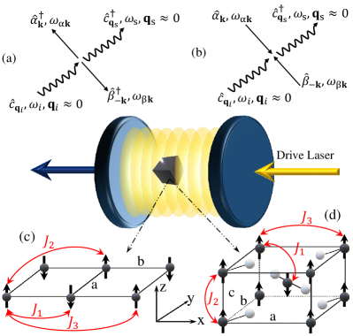
Figure 1: AFM optomagnonic cavity. Light-matter coupling within the domain of nonresonant two-magnon Raman scattering processes: (a) Stokes scattering with a redshifted frequency of $\omega_{s}=\omega_{i}-\omega_{\alpha{\bf k}}-\omega_{\beta{\bf k}}$ and (b) anti-Stokes scattering with blueshifted frequency $\omega_{as}=\omega_{i}+\omega_{\alpha{\bf k}}+\omega_{\beta{\bf k}}$. Crystal and magnetic structure of (c) the Rutile- and (d) quasi-two-dimensional AFMs. Short-range exchange constants $J_{\mathbf{R^{\prime}}}$ are defined as $J_{l}$ ($l=1,2,3$).

The rapid evolution of information technology demands devices with high storage density, energy efficiency, and fast read/write speeds. As traditional silicon-based electronics approach their physical limits, new paradigms are essential to meet the growing demands of modern technology KEYES (1981); Vashchenko and Sinkevitch (2008); Keyes (2001). Magnonics, which explores magnons — the quanta of spin waves in magnetic materials — as alternative information carriers, has emerged as a promising direction Flebus et al. (2024); Chumak et al. (2022); Baltz et al. (2018); Jungwirth et al. (2018); Spaldin (2010); Duine et al. (2018); Han et al. (2023); Jungwirth et al. (2016); Qaiumzadeh et al. (2018); Chumak et al. (2015); Chumak (2019); Wang et al. (2020); Hortensius et al. (2021). Among magnetic materials, antiferromagnets (AFMs) stand out due to their reduced magnetic noise and high-frequency operation up to the terahertz (THz) range Borovik-Romanov and Kreines (1982). Effectively manipulating and controlling magnons in AFMs is currently an active area of research. Various external stimuli, such as electrical currents Železnỳ et al. (2014); Wadley et al. (2016); Moriyama et al. (2018) and short laser pulses Wienholdt et al. (2012); Bossini et al. (2019); Olejník et al. (2018); Satoh et al. (2015); Kimel et al. (2024); Němec et al. (2018); Surynek et al. (2024), are being investigated for this purpose.

An alternative approach for magnon manipulation is to leverage the interaction with electromagnetic cavities, which enhances the coupling between magnons and confined photons Viola Kusminskiy (2019); Almpanis (2021); Rameshti et al. (2022); Lee et al. (2023); Sharma et al. (2022). While most efforts to date have concentrated on the ferrimagnetic material Yttrium Iron Garnet (YIG) coupled to microwave Zhang et al. (2014); Hisatomi et al. (2016) and optical cavities  Viola Kusminskiy et al. (2016); Liu et al. (2016); Osada et al. (2018); Liang et al. (2023); Sharma et al. (2019); Haigh et al. (2016); Šimić et al. (2020); Sharma et al. (2024), the interplay between electromagnetic cavities and antiferromagnetic magnons has begun to be explored both theoretically Parvini et al. (2020); Xiao et al. (2019); Curtis et al. (2022) and experimentally Boventer et al. (2023); Białek et al. (2021); Zhang et al. (2021a). In optical cavities, AFM magnons can predominantly couple to photons through one-magnon and two-magnon Raman scattering processes, involving three- and four-particle interactions, respectively Fleury and Loudon (1968); Fleury et al. (1966); Loudon (1968). It has been proposed that coherent, cavity-enhanced one-magnon scattering could be harnessed e.g. for magnon cooling and quantum memory protocols in Rutile-AFMs with two collinear spin sublattices (e.g., MnF₂, FeF₂, NiO) Parvini et al. (2020). However, unlike ferromagnets, two-magnon scattering in AFMs dominates their one-magnon counterpart as the former arises from the strong exchange interactions between opposite spin sublattices. Therefore, in this study, we concentrate on the regime of cavity-enhanced two-magnon Raman scattering in AFMs.

Experimental evidence demonstrates that this scattering in MnF₂ and FeF₂ is 2-3 times stronger than one-magnon Raman scattering Fleury et al. (1967); Lockwood and Cottam (1987); Cottam et al. (1983). Furthermore, in high-transition temperature ($T_{c}$) superconductors such as La₂CuO₄ and YBa₂Cu₃O₆ (with spin $S=\frac{1}{2}$), it becomes the dominant light-matter coupling mechanism within their insulating phases Lee et al. (2006); Moriya and Ueda (2003); Erlandsen et al. (2019); Canali and Girvin (1992). In the cuprate superconductors, quantum spin fluctuations play a crucial role in the electric conductivity within the CuO₂ planes Kastner et al. (1998); Betto et al. (2021); Scalapino (2012); Mitrano et al. (2016); Mankowsky et al. (2014). By creating magnon pairs Odagaki and Tani (1971); Fedianin et al. (2023), two-magnon Raman scattering can be used for generating squeezed magnon states Zhao et al. (2004), where spin fluctuations can fall below the quantum vacuum noise level. This opens exciting possibilities beyond established phonon squeezing applications Hu and Nori (1996a, b). Therefore, the interest in exploring the dynamics of an optical cavity coupled to two-magnon Raman processes is two-fold: on the one hand, this kind of interaction goes beyond the usual “optomechanical interaction” paradigm Aspelmeyer et al. (2014) (given by an interaction term of the kind $g_{0}\hat{a}^{\dagger}\hat{a}(\hat{m}+\hat{m}^{\dagger})$ where $g_{0}$ is the vacuum coupling strength, $\hat{a}^{(\dagger)}$ are the photonic annihilation (creation) operators, and, in the case of magnons, $\hat{m}^{(\dagger)}$ are the magnonic annihilation (creation) operators), where protocols for manipulation of magnon states, e.g. for cooling or the generation of quantum states, are well understood. On the other hand, the possibility of manipulating magnon states by cavity-enhanced two-magnon Raman scattering could provide insights into how to control fluctuations in strongly correlated systems supporting antiferromagnetism and their potential impact on the underlying electronic phase Erlandsen et al. (2019).

In this work, we explore the coupled dynamics of optical photons in a cavity and two-magnon processes focusing on two examples of Rutile-AFM insulators and cuprate parent compounds. The outline of the paper is as follows. In Sec. II, we present the theoretical model based on the magnon-photon interaction Hamiltonian. The emergence of magnon-pair operators within the total Hamiltonian leads us to use the Perelomov representation for magnon operators Perelomov (1975); Kastrup (2007); Novaes (2004); Aravind (1988), satisfying the commutation relations of the SU(1,1) Lie algebra Gerry (1985). We end the section by deriving the coupled equations of motion for the system in the presence of a drive laser and losses. In Sec. III we obtain effective equations of motion in the fast cavity limit, where the dynamics of the two-magnon operators are slow compared to the characteristic time scales of the cavity photons. By integrating out the photons, we obtain an optically induced (anti-) damping term, reminiscent of an anisotropic Gilbert term in the SU(1,1) space, and we show that it can surpass the intrinsic magnon dissipation, even with a modest number of circulating photons, enabling dynamic control of the Perelomov coherent states through the interplay of cavity drive and dissipation. We explore the possible attractors of the resulting nonlinear system, showing the possibility of steady-state squeezed Perelomov coherent states. In Sec. IV, we further characterize the system’s full dynamics beyond the fast cavity limit, showing the possibility of bringing the system into a chaotic attractor in the blue-detuned regime. This regime is of interest for applications in spin-torque oscillator nano-oscillators (STNOs) and unconventional signal-processing schemes Mayergoyz et al. (2009); Elyasi et al. (2020); Rezende and de Aguiar (1990); Yuan et al. (2022). In App. A we present the derivation of the AFM Hamiltonian for Rutile AFMs and cuprate parent compounds, along with the magnon frequency spectrum and density of states along the Brillouin zone. For more details on the full dynamics of magnon-pairs, we direct readers to App. B. App. C provides the derivation of the squeezing formula for Perelomov operators.

II Theoretical Model

We theoretically model a high-finesse optical cavity externally pumped by a laser, with an AFM insulator placed inside, as illustrated in Fig. 1. We focus on AFMs where the dominant coupling mechanism with optical photons arises from two-magnon Raman scattering, specifically: (i) Rutile-AFM compounds, such as XF₂ (X=Fe, Mn), and (ii) cuprate parent compounds exhibiting Mott insulating behavior, e.g. La₂CuO₄ and YBa₂Cu₃O₆ (YBCO). The spin configurations of the AFMs are shown in Fig. 1(c,d). It is important to note that the spin order in cuprates can exhibit complex structures, including in-plane, out-of-plane, and canted configurations, depending on the experimental conditions and composition Coldea et al. (2001); Bonesteel (1993); Curtis et al. (2022); Chen et al. (2011); Govind et al. (2001); Dalla Piazza (2016). However, the primary focus of this study is to formulate the system’s dynamics in the presence of an unconventional coupling mechanism, namely, the two-magnon Raman scattering process. To this end, we have adopted a simplified two-dimensional geometry, disregarding interlayer couplings and assuming an out-of-plane spin order Wan et al. (2009); Sandvik et al. (1998); Manousakis (1991); Chakravarty et al. (1989). Our work paves the way for further studies considering bilayer cuprates and more complex spin order configurations.

II.1 Microscopic Hamiltonian

We consider a spin Hamiltonian given by

$$\hat{\mathcal{H}}_{m}=\sum_{\mathbf{R}}\left[\sum_{\mathbf{R}^{\prime}}J_{\mathbf{R^{\prime}}}\hat{\boldsymbol{S}}_{\mathbf{R}}\cdot\hat{\boldsymbol{S}}_{\mathbf{R}+\mathbf{R}^{\prime}}-D\left(\hat{S}_{\mathbf{R}}^{z}\right)^{2}\right],$$ (1)

where $\hat{\boldsymbol{S}}_{\mathbf{R}}$ denotes a spin-$S$ particle located at site $\mathbf{R}$, and $J_{\mathbf{R}^{\prime}}$ is the exchange interaction between spins separated by $\mathbf{R}^{\prime}$. In the case of two-magnon Raman scattering, momentum conservation allows the excitation of magnons with any equal and opposite momentum $\bf{k}$. In our model, we consider interactions up to the third nearest neighbor, as depicted in Fig. 1, since $J_{2}$ and $J_{3}$ are relevant when considering magnons with non-zero momentum (${\bf{k}}\neq 0$), see Eq. A2 (App. A). The second term in Eq. (1) denotes an easy-axis anisotropy aligning the Néel vector along the $\boldsymbol{z}$ direction. This is associated with the anisotropy field $H_{A}$ through $D=g\mu_{B}H_{A}/(2S)$, where $g$ is the spectroscopic splitting factor and $\mu_{B}$ is the Bohr magneton. Employing a Holstein-Primakoff transformation Holstein and Primakoff (1940), applying a Fourier transformation, and a Bogoliubov transformation (see App. A), the Hamiltonian in Eq. (1) becomes

$$\hat{\mathcal{H}}_{m}=\hbar\sum_{{\bf k}}\omega_{m\mathbf{k}}\left[\alpha_{{\bf k}}^{\dagger}\alpha_{{\bf k}}+\beta_{-{\bf k}}^{\dagger}\beta_{-{\bf k}}+1\right],$$ (2)

where $\alpha_{\bf k}$ and $\beta_{\bf-k}$ ($\alpha_{\bf k}^{\dagger}$ and $\beta_{\bf-k}^{\dagger}$) are the annihilation (creation) operators of bosonic magnon modes with eigenfrequencies $\omega_{m\mathbf{k}}$. The eigenfrequencies of the considered cuprates are higher than those of Rutile-AFMs owing to the presence of stronger exchange interactions (App. A).

We consider an intercavity electric field $\hat{\mathbf{E}}=\hat{\boldsymbol{\cal E}}+\hat{\boldsymbol{\cal E}^{\dagger}}$ such that

$$\hat{\boldsymbol{\cal E}}(\mathbf{R})=i\sqrt{\frac{2\hbar\omega_{c}}{\varepsilon V}}\ \boldsymbol{p}\hat{c}e^{i\bf{q}.\bf R}.$$ (3)

Here, $\varepsilon$ and $V$ are the permittivity and volume of the cavity, respectively. $\boldsymbol{p}$, $\mathbf{q}$, $\omega_{c}$, and $\hat{c}$ denote the polarization, wavevector, resonance frequency, and annihilation operator of the cavity photon, respectively. The empty-cavity Hamiltonian is $\hat{\mathcal{H}}_{c}=\hbar\omega_{c}\hat{c}^{\dagger}\hat{c}$.

The interaction between the electric field in the cavity and the AFM is described through linear and quadratic magneto-optical couplings Cottam (1975); Cottam and Lockwood (1986); Moriya (1967). The corresponding interaction Hamiltonian is given by

$$\hat{\mathcal{H}}_{\rm int}=\sum_{\mu,\nu}\sum_{\bf{R}}\hat{\cal E}^{\mu}(\mathbf{R})\hat{\cal E}^{\nu,\dagger}(\mathbf{R})\hat{\chi}^{\mu\nu}\left(\mathbf{R}\right),$$ (4)

where $\hat{\cal E}^{\mu}(\mathbf{R})$ is the $\mu$-component of $\hat{\boldsymbol{\cal E}}$ at site $\bf{R}$ in the crystal and $\hat{\chi}^{\mu\nu}({\bf R})$ represents a component of the spin-dependent polarizability tensor,

$$\hat{\chi}^{\mu\nu}({\bf R}) =\sum_{\gamma}K_{\mu\nu\gamma}\left(\mathbf{R}\right)\hat{S}_{\mathbf{R}}^{\gamma}+\sum_{\gamma,\delta}G_{\mu\nu\gamma\delta}\left(\mathbf{R}\right)\hat{S}_{\mathbf{R}}^{\gamma}\hat{S}_{\mathbf{R}}^{\delta}$$ (5)

$$+\sum_{\gamma,\delta,\mathbf{R^{\prime}}}B_{\mu\nu\gamma\delta}\left(\mathbf{R},\mathbf{R^{\prime}}\right)\hat{S}_{\mathbf{R}}^{\gamma}\hat{S}_{\mathbf{R}+\mathbf{R^{\prime}}}^{\delta}+...,$$

where $\gamma,\delta,\mu,\nu\in\{x,y,z\}$. The magnitudes represented by $K$, $G$, and $B$ characterize magneto-optical effects Cottam (1975); Lockwood and Cottam (1987); Boström et al. (2023); Lockwood and Cottam (2012). The first two terms in Eq. (5) involve spin operators at a single site $\bf{R}$, whereas the third term involves a pair of operators at different sites. The first and second terms arise primarily from indirect electric dipole coupling mediated by spin-orbit interactions Fleury and Loudon (1968). The third term is associated with the excited-state exchange interaction and involves electric-dipole transitions. In most AFM insulators, the third term emerges as the predominant light-matter interaction Fleury et al. (1967); Fleury and Loudon (1968). This interaction can lead to a non-thermal excitation of magnon-pairs when the incident photon intensity exceeds a certain threshold Odagaki and Tani (1971); Odagaki (1973a, b). For a monochromatic photonic cavity, the principle of conservation of energy gives rise to two distinct types of two-magnon Raman scattering processes: Stokes (Fig. 1(a)) and anti-Stokes scattering (Fig. 1(b)). Raman experiments typically involve infrared to visible photons with frequencies $\sim$500\text{\,}\mathrm{THz}$$, corresponding to wavevectors $|{\bf{q}}|\sim$15\text{\,}\mathrm{\SIUnitSymbolMicro}\mathrm{m}^{-1}$$ which is significantly smaller than typical magnon momenta throughout the Brillouin zone. Consequently, this process leads to the creation of magnon-pairs with approximately opposite wave vectors Formisano et al. (2024). Group theory analysis Fleury et al. (1967); Dimmock and Wheeler (1962); Loudon (1968); Sugano and Kojima (2013); Fleury and Guggenheim (1970); Amer et al. (1975); Weber and Merlin (2000); Devereaux and Hackl (2007); Poppinger (1977); Davies et al. (1971); Vernay et al. (2007); Sandvik et al. (1998); Chubukov and Frenkel (1995) reveals that the interaction Hamiltonian for simple cubic lattices, considering only the third term in Eq. (5), simplifies to

$$\hat{\mathcal{H}}_{int}=-\sum_{\mathbf{R}\mathbf{R^{\prime}}}\frac{B}{|{\mathbf{R^{\prime}}}|^{2}}\left(\hat{\boldsymbol{\mathcal{E}}}\cdot\mathbf{R^{\prime}}\right)\left(\hat{\boldsymbol{\mathcal{E}}}^{\dagger}\cdot\mathbf{R^{\prime}}\right)\hat{\boldsymbol{S}}_{\mathbf{R}}\cdot\hat{\boldsymbol{S}}_{\mathbf{R}+\mathbf{R^{\prime}}},$$ (6)

where the variable $\mathbf{R^{\prime}}$ spans over nearest neighbors. Theoretically, the coupling coefficient $B$ in cuprates can be derived from a half-filled single-band Hubbard model, given by $B=\frac{4t^{2}}{|\hat{\cal E}|^{2}(U-\hbar\omega_{c})}$, where $t$ represents the hopping amplitude between nearest neighbor sites, and $U$ is the on-site electron-electron interaction Shastry and Shraiman (1990); Canali and Girvin (1992). For Rutiles, its derivation from time-dependent perturbation theory is detailed in Fleury and Loudon (1968); Fleury et al. (1967). From an experimental perspective, the exact value of $B$ in Rutiles is not known (we only have ratios between different scattering geometries Zhao et al. (2006); Fleury and Loudon (1968)) whereas, for cuprates, $U$ and $t$ have been obtained by connecting spectroscopic measurements to the microscopic model Sheshadri et al. (2023).

II.2 Coupling constants

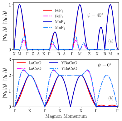
Figure 2: The magnitudes of the coefficients $\mathcal{R}_{\bf k}$ (dash-dot lines) and $\mathcal{T}_{\bf k}$ (solid lines), normalized to the coupling constant, at different wave-vectors for (a) Rutile-AFMs and (b) cuprates-AFMs. See Figs. 9(b) and 10(b) for the definitions of the wave-vector points on the x-axis.

This subsection discusses the effective interaction Hamiltonian for a given light polarization. Our analysis focuses on single-mode cavities with electric fields linearly polarized in the XY plane, described by the polarization vector

$$\mathbf{p}=\cos\psi\mathbf{x}+\sin\psi\mathbf{y}.$$ (7)

This specific choice is motivated by studies showing strong two-magnon Raman scattering in this geometry Zhao et al. (2006); Lockwood and Cottam (2012, 1987); Fleury et al. (1967); Sandvik et al. (1998); Cottam et al. (1983). Expanding spins in the magnon basis, the interaction Hamiltonian in Eq. (6) becomes

$$\hat{\mathcal{H}}_{\rm int} =\hbar\sum_{{\bf k}}\left[\mathcal{R}_{{\bf k}}\left(\hat{\alpha}_{{\bf k}}^{\dagger}\hat{\alpha}_{{\bf k}}+\hat{\beta}_{-\mathbf{k}}^{\dagger}\hat{\beta}_{-{\bf k}}+1\right)\right.$$ (8)

$$\qquad\qquad\left.+\mathcal{T}_{{\bf k}}\left(\hat{\alpha}_{{\bf k}}\hat{\beta}_{-{\bf k}}+\hat{\alpha}_{\mathbf{k}}^{\dagger}\hat{\beta}_{-\mathbf{k}}^{\dagger}\right)\right]\hat{c}^{\dagger}\hat{c},$$

where $\mathcal{R}_{{\bf k}}=-\mathcal{G}\Pi_{\mathcal{R},\bf{k}}^{xy}\sinh\theta_{{\bf k}}$, $\mathcal{T}_{{\bf k}}=\mathcal{G}\Pi_{\cal{T},\bf{k}}^{xy}\cosh\theta_{{\bf k}}$ and $\theta_{\bf k}$ is the Bogoliubov angle defined in App. A quantifying the two-mode squeezing between the two sublattices. The coupling factor is given by

$$\mathcal{G}=2B\left(\frac{a}{d_{\rm neigh}}\right)^{2}\frac{\omega_{c}S}{\varepsilon V},$$ (9)

where $d_{\rm neigh}$ is the nearest neighbor distance, given by $\sqrt{2a^{2}+c^{2}}/2$ for rutile-AFMs and by $a$ for 2D cuprates, with $a$ and $c$ being the lattice constants, see App. A. To simplify calculations, we assumed equal cavity and AFM volumes as $V$. In reality, the filling factor (ratio of AFM to cavity volume) is crucial, as it significantly affects the light-matter interaction strength Weichselbaumer et al. (2019); Graf et al. (2021).

The factor $\Pi^{xy}$ encodes the dependence on the lattice structure and the optical polarization, which will be discussed in the following subsections. Eq. (8) shows that the two-photon two-magnon light-matter interaction not only leads to the creation and annihilation of magnon-pairs (governed by the $\mathcal{T}_{{\bf k}}$ coefficient) but also induces frequency shifts (governed by the $\mathcal{R}_{{\bf k}}$ coefficient). For Rutile-AFMs, we have

$$\Pi_{{\cal T},\mathbf{k}}^{xy}=\Pi_{{\cal R},\mathbf{k}}^{xy}=\sin 2\psi\sin\left(\frac{ak_{x}}{2}\right)\sin\left(\frac{bk_{y}}{2}\right)\cos\left(\frac{ck_{z}}{2}\right),$$

and for 2D cuprates

$$\Pi_{{\cal T},\mathbf{k}}^{xy} =2\left[\cos^{2}\psi\cos\left(ak_{x}\right)+\sin^{2}\psi\cos\left(ak_{y}\right)-\tanh(\theta_{{\bf k}})\right]$$

$$\Pi_{{\cal R},\mathbf{k}}^{xy} =2\left[\cos^{2}\psi\cos\left(ak_{x}\right)+\sin^{2}\psi\cos\left(ak_{y}\right)-\coth(\theta_{{\bf k}})\right].$$

These expressions show that Rutile-AFMs exhibit maximum coupling at a polarization angle of $\psi=\pi/4$, whereas cuprates achieve maximum coupling at $\psi=0^{\circ}$ or $\psi=\pi/2$. Fig. 2 illustrates the variation of $\mathcal{R}_{\bf k}$ and $\mathcal{T}_{\bf k}$ in wavevector space, revealing that $\mathcal{T}$ peaks at the M-point for Rutile-AFMs and at the X-point for cuprates. Notably, at these points, the magnon density of states (DOS) exhibits a significant peak closely associated with van Hove singularities, as shown in Figs. 9(d) and 10(d). This suggests that these wavevectors—the M-point for Rutile and the X-point for cuprates—play a dominant role in light-matter coupling. Consequently, we focus our analysis on these dominant wavevectors. Neglecting the $\mathbf{k}$-index, the total effective Hamiltonian can be expressed as:

$$\frac{\hat{\mathcal{H}}}{\hbar} =\omega_{c}\hat{c}^{\dagger}\hat{c}+\omega_{m}\left[\alpha^{\dagger}\alpha+\beta^{\dagger}\beta+1\right]+\left[\mathcal{R}\left(\hat{\alpha}^{\dagger}\hat{\alpha}+\hat{\beta}^{\dagger}\hat{\beta}+1\right)\right.$$

$$\quad\left.+\mathcal{T}\left(\hat{\alpha}\hat{\beta}+\hat{\alpha}^{\dagger}\hat{\beta}^{\dagger}\right)\right]\hat{c}^{\dagger}\hat{c}.$$ (10)

II.3 Perelomov representation

As discussed in the previous section, within our model magnon excitations exclusively manifest in pairs of $\hat{\alpha}_{\bf k}$ and $\hat{\beta}_{-\bf k}$ magnons. This observation leads us to rewrite the Hamiltonian based on two-magnon or equivalently Perelomov operators defined by Novaes (2004); Gerry et al. (1991); Gerry (1985)

$$\hat{K}^{+} =\hat{\alpha}^{\dagger}\hat{\beta}^{\dagger},\qquad\hat{K}^{-}=\hat{\alpha}\hat{\beta},$$ (11)

$$\hat{K}^{z} =\frac{1}{2}\left(\hat{\alpha}^{\dagger}\hat{\alpha}+\hat{\beta}^{\dagger}\hat{\beta}+1\right),$$

which fulfill the commutation relations of a SU(1,1) Lie algebra: $\left[\hat{K}^{z},\hat{K}^{\pm}\right]=\pm\hat{K}^{\pm}$ and $\left[\hat{K}^{-},\hat{K}^{+}\right]=2\hat{K}^{z}$ with $\hat{K}^{\pm}=\hat{K}^{x}\pm i\hat{K}^{y}$. The Casimir operator $\hat{C}=({\hat{K}}^{z})^{2}-\frac{1}{2}({\hat{K}}^{+}{\hat{K}}^{-}+{\hat{K}}^{-}{\hat{K}}^{+})$ which commutes with all $\hat{K}$ operators, is a constant of motion. In this representation, the Hamiltonian in Eq. (10) reads

$$\frac{\hat{\mathcal{H}}}{\hbar}=\omega_{c}\hat{c}^{\dagger}\hat{c}+2\omega_{m}\hat{K}^{z}+\hat{\cal K}\hat{c}^{\dagger}\hat{c},$$ (12)

where we have defined

$$\hat{\cal K}=2{\cal R}\hat{K}^{z}+2{\cal T}\hat{K}^{x}.$$ (13)

For future convenience, we can also write Eq. (13) as $\hat{\cal K}=2\mathbf{e}\,\underline{\boldsymbol{\cdot}}\,\hat{\mathbf{K}}$ with $\mathbf{e}={\cal T}\mathbf{x}-{\cal R}\mathbf{z}$, $\hat{\mathbf{K}}$ is the vector $(K^{x},K^{y},K^{z})$ and we define a scalar product in SU(1,1) as $\mathbf{a}\,\underline{\boldsymbol{\cdot}}\,\mathbf{b}=a_{x}b_{x}+a_{y}b_{y}-a_{z}b_{z}$.

The SU(1,1) basis states are $|m,k\rangle$ such that $\hat{K}^{z}|m,k\rangle=(m+k)|m,k\rangle$ where $m=0,1,2,\ldots$ and $k$ is the Bargmann index. The eigenvalues of the Casimir operator $\hat{C}=(\hat{K}^{z})^{2}-(\hat{K}^{x})^{2}-(\hat{K}^{y})^{2}$ are $k(k-1)$ with $k>0$. Using Eq. (11), we can show the relation $2k-1=|n_{\alpha}-n_{\beta}|$ where $n_{\alpha,\beta}$ are the number of $\{\alpha,\beta\}$-magnons.

The SU(1,1) Perelomov coherent states are defined as  Aravind (1988); Robert and Combescure (2021); Perelomov (1972); Gerry and Kiefer (1991)

$$|\zeta,k\rangle=S(z)|0,k\rangle,$$ (14)

where

$$S(z)=\exp(zK^{+}-z^{*}K^{-}),$$ (15)

and $z=-(\theta/2)e^{-i\phi}$, $\zeta=-\tanh\left(\frac{\theta}{2}\right)e^{-i\phi}$. The angles $\theta$ and $\phi$ parametrize the SU(1,1) group manifold and have ranges $-\infty<\theta<\infty$ and $0\leq\phi\leq 2\pi$.

The expectation values of $\hat{K}^{x,y,z}$ in Perelomov coherent states, denoted as $K^{i}\equiv\langle\hat{K}^{i}\rangle_{\text{PCS}}$, are:

$$K^{z}=K\cosh\vartheta,\quad K^{x}-iK^{y}=K\sinh\vartheta e^{-i\varphi},$$ (16)

where the squares of the expectation values fulfill the relation:

$$(K^{x})^{2}+(K^{y})^{2}-(K^{z})^{2}=const.,$$ (17)

or in the notation of the SU(1,1) dot product, $K^{2}=-\mathbf{K}\,\underline{\boldsymbol{\cdot}}\,\mathbf{K}$, where we define the vector $\mathbf{K}=(K^{x},K^{y},K^{z})$. Using the definition of the Casimir operator above, we can interpret Eq. (17) as the constancy of the difference of number of $\alpha$ and $\beta$ magnons. In what follows we will obtain the equations of motion for the expectation values of the Perelomov operators.

II.4 Coupled equations of motion for a driven system

In this subsection, we derive the coupled Langevin equations of motion for photons and magnons governed by the Hamiltonian Eq. (12), adding a driving source for the cavity and dissipation for both the cavity and magnons.

We consider a cavity subject to an input pump laser with an amplitude of $s_{d}$ and a frequency of $\omega_{d}$, giving an input power of $P_{d}=\hbar\omega_{d}s_{d}^{2}$. Using input-output theory Gardiner and Collett (1985), the equation of motion for the intracavity photon field in the rotating frame of the drive can be written as

$$\frac{d\hat{c}}{dt}=-i\left(\Delta+\hat{\cal K}-\frac{i\kappa}{2}\right)\hat{c}+\sqrt{\rho\kappa}s_{d}+\sqrt{\kappa}\hat{c}_{\text{noise}},$$ (18)

where $\Delta=\omega_{c}-\omega_{d}$ is the drive detuning, $\kappa$ is the cavity linewidth including intrinsic and extrinsic damping, $\rho$ is the ratio of extrinsic to intrinsic damping, $\hat{c}_{\rm noise}$ is the vacuum noise satisfying $\langle\hat{c}_{\rm noise}\rangle=0$, and $\hat{\cal K}$ is defined in Eq. (13). The dynamics of the magnon annihilation operators are given by

$$\frac{d\hat{\xi}}{dt}=\frac{i}{\hbar}\left[\hat{\cal H},\hat{\xi}\right]-\frac{\kappa_{G}}{2}\hat{\xi}-\sqrt{\kappa_{G}}\hat{\xi}_{\rm noise},$$ (19)

where $\xi\in\{\alpha,\beta\}$ represents one of the magnon modes, $\hat{\xi}_{\rm noise}$ is the bath noise for the $\xi$-magnons, and $\kappa_{G}$ is the intrinsic Gilbert damping, which is the same for both modes  Cottam et al. (1983); Rezende (2020). The noise satisfies the standard correlation functions Breuer and Petruccione (2002); Ángel Rivas and Huelga (2012): $\langle\xi_{\rm noise}(t)\rangle=0$ and $\langle\xi_{\rm noise}^{\dagger}(t)\xi_{\rm noise}(t^{\prime})\rangle=n_{\rm th}\delta(t-t^{\prime})$ where $n_{\rm th}$ is the Bose-Einstein distribution at ambient temperature.

From this, we can derive the equations of motion for the magnon-pair operators,

$$\frac{d\left\langle\hat{K}^{i}\right\rangle}{dt}=\frac{i}{\hbar}\left\langle\left[\hat{{\cal H}},\hat{K}^{i}\right]\right\rangle-\kappa_{G}\left(\left\langle\hat{K}^{i}\right\rangle-\frac{\delta_{iz}}{2}\right),$$ (20)

where $i\in{x,y,z}$ and expectations are taken over Perelomov coherent states.

In the following, we discuss the semi-classical equations of motion where we ignore quantum correlations between the spins and the photons, i.e. we approximate $\langle\hat{c}\hat{\cal K}\rangle\approx\langle\hat{c}\rangle\langle\hat{\cal K}\rangle$. $\langle\hat{\cal K}\rangle$ is the expectation value of the $\mathbf{K}$-vector in Perelomov coherent states, as explained in Sec. II.3. Defining the averages $c=\langle\hat{c}\rangle$ and $\mathcal{K}=\langle\hat{\cal K}\rangle$ (along with $K^{x,y,z}$ defined above), we can write the coupled semi-classical equations of motion as

$$\frac{dc}{dt}=-i\left(\Delta+{\cal K}-\frac{i\kappa}{2}\right)c+\sqrt{\rho\kappa}s_{d},$$ (21)

and

$${\dot{\bf K}}={\bf{\Omega}}\underline{\times}\mathbf{K}-\kappa_{G}\left(\mathbf{K}-\frac{\bf z}{2}\right),$$ (22)

where $\mathbf{\Omega}=2\omega_{m}\mathbf{z}-2\mathbf{e}|c|^{2}$ with $\mathbf{e}$ defined below Eq. (12). The vector product $\underline{\times}$ in SU(1,1) is defined as

$$\mathbf{a}\underline{\times}\mathbf{b}=\begin{pmatrix}a_{y}b_{z}-a_{z}b_{y}\\ a_{z}b_{x}-a_{x}b_{z}\\ a_{y}b_{x}-a_{x}b_{y}\end{pmatrix}.$$ (23)

It differs from the standard cross-product in the sign of the $z$-component.

III Fast cavity regime

In this section, we discuss the fast cavity limit, corresponding to $\kappa^{2}\gg\dot{\cal K}$, wherein we can solve the optical equations of motion adiabatically by treating the pseudospin operators parametrically. This allows us to eliminate photons to obtain an effective equation of motion only for the pseudospin in Sec. III.1. Using this equation, we discuss the fixed points and the stability of magnons in Sec. III.2. Finally, we discuss numerical simulations showing the time evolution of magnons in Sec. III.3.

III.1 Effective equation of motion

We can find $c(t)$ in terms of $\mathcal{K}(t)$ following a procedure analogous to Viola Kusminskiy et al. (2016), where the coupling of light to a SU(2) spin was studied. We expand the photon field in terms of time derivatives of $\mathcal{K}$,

$$c(t)=c_{0}(t)+c_{1}(t)+\ldots$$ (24)

where the index $i$ of the $c_{i}$ terms indicates the derivative order. For example, the second order term $c_{2}$ consists of $\dot{\cal K}^{2}$ and $\ddot{\cal K}$.

In steady state, $\dot{c}=0$. Using Eq. (21), the zeroeth order contribution reads

$$c_{0}(t)=\frac{\sqrt{\rho\kappa}s_{d}}{i\left(\Delta+{\cal K}(t)-\frac{i\kappa}{2}\right)}.$$ (25)

To find the first order correction $c_{1}$, we note that the time derivative $\dot{c}_{1}$ is a second order term and thus can be ignored, giving

$$c_{1}(t)=\frac{-ic_{0}(t)}{\left(\Delta+{\cal K}(t)-\frac{i\kappa}{2}\right)^{2}}\dot{\mathcal{K}}(t).$$ (26)

The number of photons circulating in the cavity is given by $n_{c}=\left|c\left(t\right)\right|^{2}$ which can be approximated as $\left|c(t)\right|^{2}\approx\left|c_{0}(t)\right|^{2}+c_{0}^{*}(t)c_{1}(t)+c_{1}^{*}(t)c_{0}(t)$. Explicitly,

$$n_{c}\approx|c_{0}|^{2}\left[1+\frac{2\kappa\left(\Delta+{\cal K}\right)\dot{\mathcal{K}}}{D({\cal K})^{2}}\right],$$ (27)

where we have defined $D({\cal K})=\left(\Delta+\mathcal{K}\right)^{2}+\kappa^{2}/4$.

Substituting Eq. (27) into the equations of motion for the pseudospin vector $\mathbf{K}$, Eq. (22), gives

$$\dot{\mathbf{K}}=\boldsymbol{\Omega}_{\text{eff}}\underline{\times}\mathbf{K}-\eta_{\text{opt}}\frac{\mathbf{e}\,\underline{\boldsymbol{\cdot}}\,\dot{\mathbf{K}}}{|\mathbf{e}|^{2}}\left(\mathbf{e}\underline{\times}\mathbf{K}\right)-\kappa_{G}\left(\mathbf{K}-\frac{\boldsymbol{z}}{2}\right),$$ (28)

where $\boldsymbol{\Omega}_{\rm eff}=2\omega_{m}\mathbf{z}-2\mathbf{e}|c_{0}|^{2}$ includes the two-magnon frequency shift due to the instantaneous interaction with the cavity field, and $\eta_{\text{opt}}$ is an optically induced dissipation due to dynamical backaction and is given by

$$\eta_{\text{opt}}(\mathbf{K})=8\kappa\left(\mathcal{T}^{2}+\mathcal{R}^{2}\right)\left|c_{0}\right|^{2}\frac{\left(\Delta+2\mathbf{e}\,\underline{\boldsymbol{\cdot}}\,\mathbf{K}\right)}{D(\mathcal{K})^{2}}.$$ (29)

Within this approximation, light induces a cooperative dissipation of magnon-pairs. The form of damping has similarities with the Gilbert damping term $\alpha_{G}\dot{\mathbf{S}}\times\mathbf{S}$, well known in SU(2) spin dynamics Gilbert (2004). The sign of $\eta_{\rm opt}$ depends on the pseudospin components $K^{i}$ and the detuning of the optical drive $\Delta$. The pseudospin decays for $\eta_{\rm opt}>0$, while $\eta_{\rm opt}<0$ leads to an amplification of the pseudospin ultimately limited by nonlinearities. We discuss these conditions in more detail in the following section.

III.2 Stability of the steady state

In this section, we discuss the fixed points of the pseudospin governed by the equilibrium points of the effective equation of motion, Eq. (28). The damping rate in typical insulating AFMs is very small ($\sim$1\text{\,}\mathrm{GHz}$$ POPPINGER (1977); Lockwood and Cottam (1987); Ohlmann and Tinkham (1961); Barak et al. (1980); Cottam et al. (1983); Kotthaus and Jaccarino (1972); Vaidya et al. (2020)) and thus, to focus on the optically induced dynamics, we consider time evolutions at time scales much smaller than $\kappa_{G}^{-1}$. At such times, the quasi-equilibrium condition for the pseudospin vector is given by $\boldsymbol{\Omega}_{\rm eff}\underline{\times}\mathbf{K}_{e}=0$ implying $\mathbf{K}_{e}\propto\boldsymbol{\Omega}_{\rm eff}$. $\mathbf{K}_{e}$ indicates the quasi-equilibirum value of the pseudospin. The normalization is set by the initial condition via the conservation law $\mathbf{K}(t)\,\underline{\boldsymbol{\cdot}}\,\mathbf{K}(t)=-K^{2}$ satisfied by Eq. (28) when the Gilbert term is ignored. The equilibrium pseudospin lies in the x-z plane as $\boldsymbol{\Omega}_{\rm eff}\cdot\mathbf{y}=0$. Using the definitions for the coherent state given in Eq. (16), in equilibrium we obtain $\varphi_{e}=\pi$ and

$$\tanh\vartheta_{e}=\frac{\mathcal{T}|c_{0}|^{2}}{\omega_{m}+\mathcal{R}|c_{0}|^{2}}.$$ (30)

We see that if $\mathcal{T}>\mathcal{R}$, i.e. two-magnon scattering is stronger than the light-induced frequency shift of magnons, for a sufficiently large number of photons we get an$\tanh\vartheta_{e}>1$. Physically, this implies that the system becomes unstable Odagaki (1973b). To assess the stability of the system, we linearize the equations of motion around the equilibrium point by setting $K^{i}=K^{i}_{e}+\delta K^{i}$. In the resulting dynamical matrix for $\delta K^{i}$, the eigenvalues should be non-positive for the system to be stable. One eigenvalue of the dynamical matrix is always zero because of the conservation law $K=\text{const.}$ The other two eigenvalues $\lambda_{\pm}$ satisfy

$$\lambda_{+}+\lambda_{-} =-\eta_{e}\frac{2\omega_{m}{\cal T}\left({\cal T}K_{e}^{z}-{\cal R}K_{e}^{x}\right)}{{\cal T}^{2}+{\cal R}^{2}},$$ (31)

$$\lambda_{+}\lambda_{-} =\left(\omega_{m}+{\cal R}|c_{0}|^{2}\right)^{2}-|c_{0}|^{4}{\cal T}^{2}$$

$$\phantom{=}-\left({\cal T}K_{e}^{z}-{\cal R}K_{e}^{x}\right){\cal T}\omega_{M}\frac{\partial|c_{0}|^{2}}{\partial\mathcal{K}},$$

where $\eta_{e}\equiv\eta_{\rm opt}(\mathbf{K}_{e})$ is the damping constant at equilibrium.

For stability, $\lambda_{+}\lambda_{-}>0$ which is satisfied for small photon numbers. Moreover, $\lambda_{+}+\lambda_{-}<0$ implying $\eta_{e}>0$ that corresponds to $\Delta>-2\mathbf{e}\,\underline{\boldsymbol{\cdot}}\,\mathbf{K}$. At the equilibrium point $\mathbf{K}_{e}\propto\boldsymbol{\Omega}_{\rm eff}$ with $K_{e}^{x}\leq 0$, the condition $\eta_{e}>0$ is never fulfilled for blue-detuning $\Delta<0$. We can therefore conclude that there are no fixed point attractors at blue-detuning. For red-detuning $\Delta>0$, there can be fixed point attractors when $\eta_{e}>0$ is fulfilled.

III.3 Numerical simulations

In this section, we numerically analyze the nonlinear dynamics of the pseudospin $\mathbf{K}$ governed by Eq. (28) and guided by the stability analysis from the previous subsection. To facilitate the numerical analysis, parameters $\Delta$, $\cal T$, $\cal R$, $\kappa$, and $\kappa_{G}$ are expressed in dimensionless units of $2\omega_{m}$ with primes, such as $\Delta^{\prime}=\Delta/(2\omega_{m})$. Moreover, we define time $t^{\prime}=2\omega_{m}t$ and light amplitude ${\tilde{s}}_{d}=s_{d}\sqrt{\rho/2\omega_{m}}$. We neglect the magnon frequency shift induced by two-magnon Raman scattering, as it is negligible compared to the inherent magnon frequencies (${\cal R}^{\prime}\ll 1$). Future work can explore its influence. To have an estimation of ${\cal T}^{\prime}$ in Rutiles, we consider $B\approx 0.5\times 10^{-20}$ Peng and Hao (2004) and a refractive index $n\approx 1.5$ Jahn (1973), a cavity frequency of 650 THz, and a volume $V=10^{-18}\,\text{m}^{3}$, resulting in ${\cal T}^{\prime}\approx 0.2$ for magnons at the M-point. In cuprates, where $\mathcal{G}$ is approximated as $SJ_{1}$, numerical evaluations lead to ${\cal T}^{\prime}={\cal R}^{\prime}=0.2-0.3$ for magnons at the X-point. We set ${\cal T}^{\prime}\approx 0.2$ and ${\cal R}^{\prime}\approx 0$ for computational simplicity and compatibility across both materials.

The time evolution of $K_{x}$, $K_{z}$, $\eta_{\text{opt}}$, and $\Omega_{\text{opt}}^{x}$ under a red-detuned pump ($\Delta^{\prime}=1$) and varying drive power (${\tilde{s}}_{d}$) in the fast cavity limit is illustrated in Fig. 3. Below a threshold power, chosen as the maximum value of $\tilde{s}_{d}$ in the plots, the system dynamics resemble those of a damped harmonic oscillator, where after several oscillations, the K-components settle at specific equilibrium values, indicating a constant number of magnon pairs. For the input amplitudes chosen here, $\Delta-2{\cal T}|c_{0}|^{2}>0$ is fulfilled implying $\eta_{e}>0$. Looking at the stability conditions given in Eqs. (31), $\eta_{e}>0$ implies $\lambda_{+}+\lambda_{-}>0$. However, beyond this power threshold, the product of eigenvalues can become negative $\lambda_{+}\lambda_{-}<0$ making the fixed point unstable. This behavior is shown in Fig. 4, where we considered two power levels: one below the threshold in the plot (a) and one above the threshold in plot (b). As seen in Fig. 4(b), above the threshold, the pseudospin undergoes undamped oscillations with increasing amplitude over time, signifying a growing instability in the system. This behavior indicates that the magnon number continues to rise and does not settle into an equilibrium value. The photon number is maximized at $K^{x}=0$ (see Eq. (25)), at which point a sharp spike in $K^{z}$ and $K^{y}$ occurs. The optically induced damping ($\eta_{\rm opt}$) and rotation ($\Omega^{x}_{\rm eff}$) show oscillations. The transition from stable to unstable behavior as the drive power increases is analogous to a bifurcation in dynamical systems theory Jezek and Hernandez (1990); Chen et al. (2000). This suggests the potential for rich dynamical phases as we explore different pump parameters, opening avenues for phase control and transitions, especially in quantum materials for quantum information applications and material studies Collado et al. (2018); Zhang et al. (2021b).

In the blue-detuned regime, $\Delta^{\prime}=-1$, the $K$-components do not settle into stable equilibrium values; instead, they continuously increase over time due to the persistent energy injection from the pump laser.

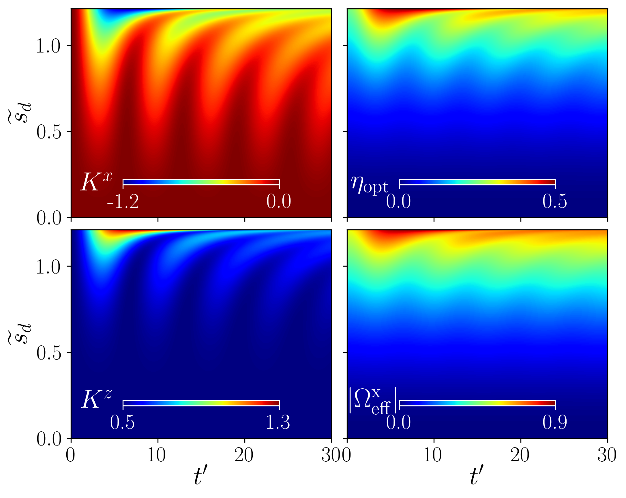
Figure 3: $K_{x}$, $K_{z}$, $\mathrm{\eta_{opt}}$, and $\Omega_{\rm opt}^{x}$ as functions of the drive field power and time in the fast cavity regime. The initial conditions for all the simulations are $K^{z}=1/2$ and $K^{x}=K^{y}=0$. The parameters are $\Delta^{\prime}=1$ (red-detuned), $\kappa^{\prime}=2$, $\mathcal{T}^{\prime}=0.2$, $\mathcal{R}^{\prime}=0$, $\kappa_{G}^{\prime}=0$ and $\rho=0.5$. Here we sweep $\tilde{s}_{d}$ from zero up to the threshold where the system becomes unstable, determined as $\tilde{s}_{d}=1.2126$. For a light frequency $\omega_{c}=650$THz and a magnon frequency either at the M- or X-points this corresponds to input powers of $P_{d}\approx 3.5\mu W$ and $P_{d}\approx 9.3\mu W$ respectively.

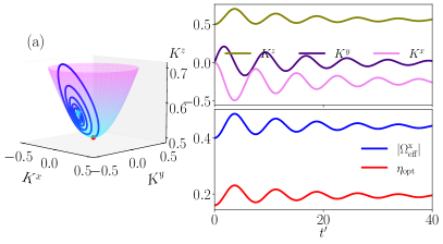
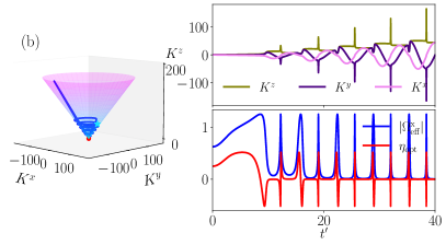
Figure 4: Trajectories of the pseudospin tip on the upper hyperboloid sheet, along with the temporal evolution of the pseudospin tip coordinates, as well as the time-dependent profiles of the optically induced frequency shift ($|\Omega_{\rm eff}^{x}|$) and dissipation coefficient ($\eta_{\rm opt}$). For (a) ${\tilde{s}}_{d}=1.0$ (below power threshold) and (b) ${\tilde{s}}_{d}=1.25$ (above power threshold). The red sphere and star mark the start and end of the trajectory, respectively. Parameters are similar to those in Fig.3.

III.4 Squeezing

The Perelomov coherent states, defined in Eq. (11), generated optically are squeezed Kastrup (2007); Aravind (1988); Bossini et al. (2019); Perelomov (1972) in the following sense. The two noncommuting quadrature operators, $\hat{K}^{x}$ and $\hat{K}^{y}$ satisfy the Heisenberg uncertainty relation $2\sigma_{K^{x}}\sigma_{K^{y}}\geq|\braket{\hat{K}^{z}}|$, where the standard deviation is defined as

$$\sigma_{K^{i}}^{2}=\left\langle\left(\hat{K}^{i}\right)^{2}\right\rangle-\left\langle\hat{K}^{i}\right\rangle^{2},$$ (32)

for $i\in\{x,y\}$. We define the squeezing factors as

$$q^{i}=\frac{\sigma_{K^{i}}^{2}-\frac{1}{2}\left|\left\langle\hat{K}^{z}\right\rangle\right|}{\frac{1}{2}\left|\left\langle\hat{K}^{z}\right\rangle\right|},$$ (33)

A state is squeezed when either $q^{x}<0$ or $q^{y}<0$. These factors are calculated for Perelomov coherent states in App. C to be,

$$\sigma_{K^{i}}^{2}=\frac{1+\left(K^{i}\right)^{2}}{2}.$$ (34)

In terms of $\vartheta$ and $\varphi$, see Eq. (16), we find

$$q^{x}=\frac{4\sinh^{2}(\vartheta/2)}{\cosh\vartheta}\left(\cosh^{2}\frac{\vartheta}{2}\cos^{2}\varphi-\frac{1}{2}\right),$$ (35)

while the same expression gives $q^{y}$ by replacing $\cos\varphi\rightarrow\sin\varphi$. The maximum squeezing corresponds to $q^{i}=-1$ ($i\in\{x,y\}$). In this regime, $q^{x}$ exhibits a positive value. In Fig. 5, we present the dependence of the squeezing factor ($q^{y}$) and equilibrium magnon-pair numbers ($K_{e}^{z}$) on drive field power for four sets of parameters ($\mathcal{T}^{\prime}$, $\kappa^{\prime}$). As drive power increases, $K_{e}^{z}$ rises and $q^{y}$ decreases, reaching a maximum and minimum, respectively, at the power threshold. However, above the threshold, $K_{e}^{z}$ goes to infinity and $q^{y}$ jumps to positive values, indicating anti-squeezing or increased fluctuations, which means the system is out of equilibrium. Moreover, for a given value of $\mathcal{T}^{\prime}$, a larger cavity damping results in a higher threshold power, a larger magnon pair population, and a smaller squeezing factor.

Magnon squeezing in AFM insulators reduces spin fluctuations within the crystallographic unit cell below the level of the vacuum fluctuation Zhao et al. (2004). This noise reduction paves the way for coherent control of spin dynamics in AFMs, potentially enabling robust quantum memories and spin-based quantum computing platforms Yuan et al. (2021); Römling and Kamra (2024); Wang et al. (2024); Makihara et al. (2021); Azimi Mousolou et al. (2020). Furthermore, the diagonal components of the spin susceptibility tensor, $\chi_{ii}$ ($i=x,y,z$), are directly proportional to spin-component fluctuations, as described by the fluctuation-dissipation theorem Kubo (1966); Abaimov (2015). In magnon-squeezed states, the spin susceptibility reaches a local minima along the squeezed direction. This effect may extend to the electrical susceptibility $\chi_{e}$ due to spin-charge coupling in strongly correlated systems, though this requires further investigation. During squeezed state generation, suppressed spin fluctuations may influence magnon-phonon scattering, magnon-magnon interactions, and superconducting mechanisms, all of which merit further experimental and theoretical studies.

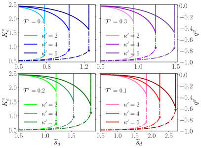
Figure 5: $K^{z}_{e}$ component of pseudospin (dash-dotted line) and squeezing factor $q^{y}$ (solid line) as a function of the drive laser power in the fast cavity regime for different $\mathcal{T}^{\prime}$ and $\kappa^{\prime}$.

IV Full Dynamic Response

In this section, we numerically solve the coupled system of nonlinear differential equations (Eqs. (18,22)) to explore the full dynamics of the system. We consider three detunings $\Delta^{\prime}\in\{1,0,-1\}$ respectively red, zero, and blue-detuning. Our numerical simulations reveal rich dynamics, including fixed points, limit cycles, and chaotic behavior, depending on the input power and detuning.

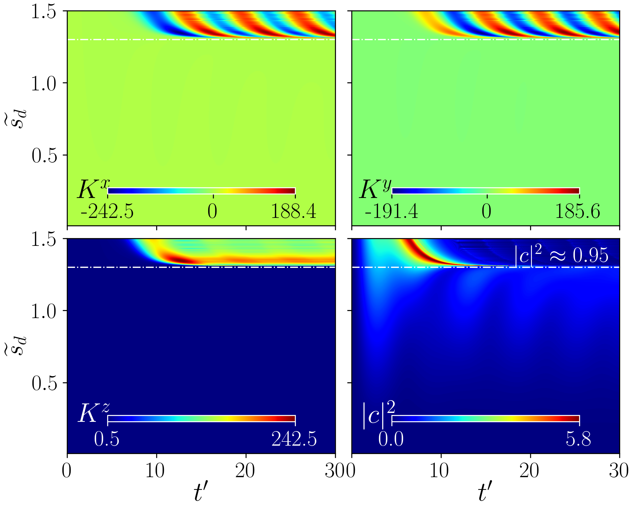
Figure 6: Temporal evaluation of pseudospin components and the photon field under varying drive power $\tilde{s}_{d}$, for red-detuning $\Delta^{\prime}=1$. We use similar parameters as in Fig. 3 except for a smaller cavity linewidth: $\kappa_{G}^{\prime}=10^{-4}$, $\kappa^{\prime}=0.5$, $\mathcal{T}^{\prime}=0.2$, and $\mathcal{R}^{\prime}=0$. Dashed lines show a threshold power ${\tilde{s}}_{d}\approx 1.3$ (corresponding to power $P_{d}\approx 4.0\mu W$ and $P_{d}\approx 10.7\mu W$ respectively for magnon frequency of M- and X-points, for $\omega_{c}=650$THz and $\rho=0.5$) below which the dynamics reach a fixed point.

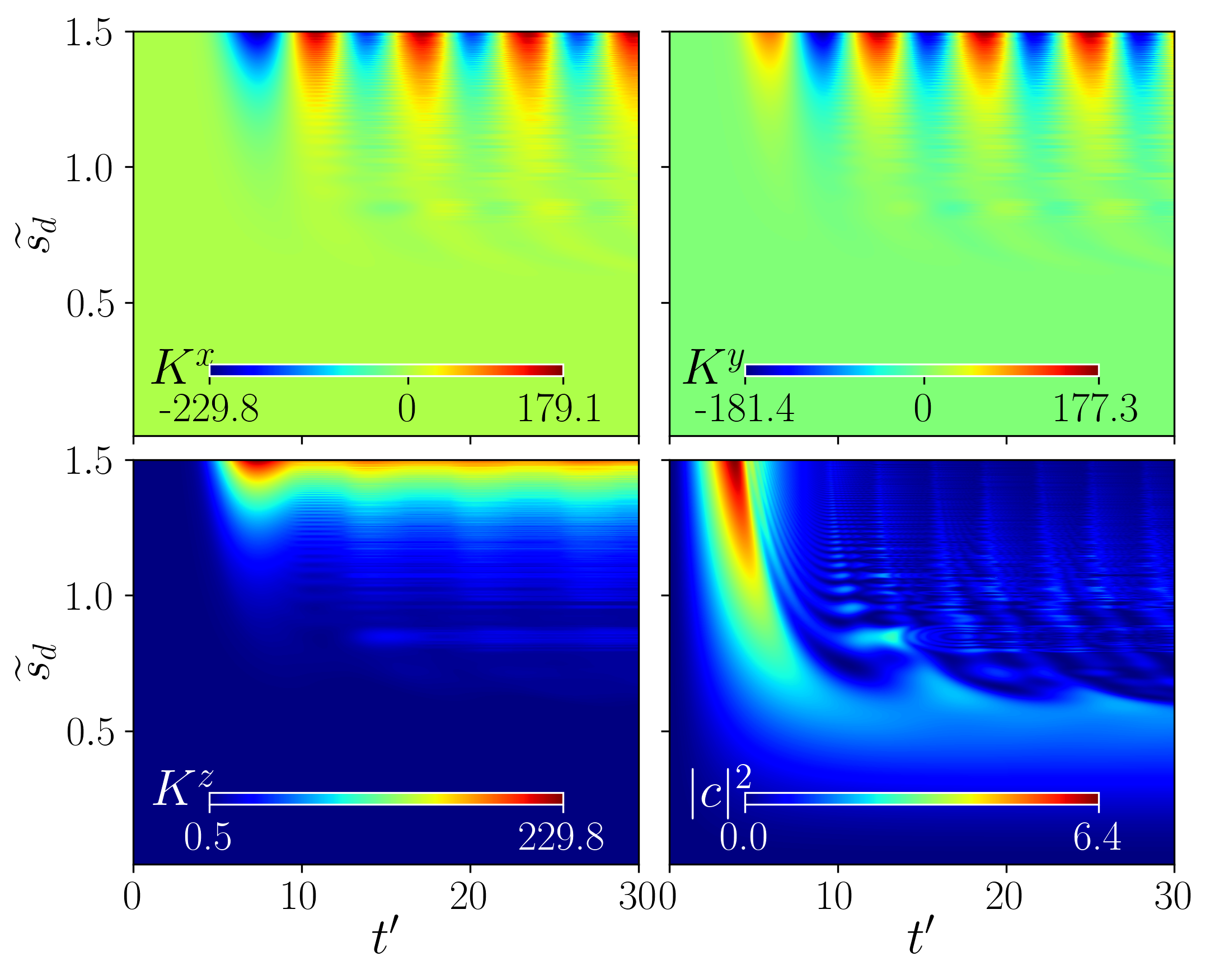
Figure 7: Temporal evaluation of pseudospin components and the photon field under varying drive power, $\tilde{s}_{d}$ for a resonant input $\Delta^{\prime}=0$ with parameters as in Fig. 6

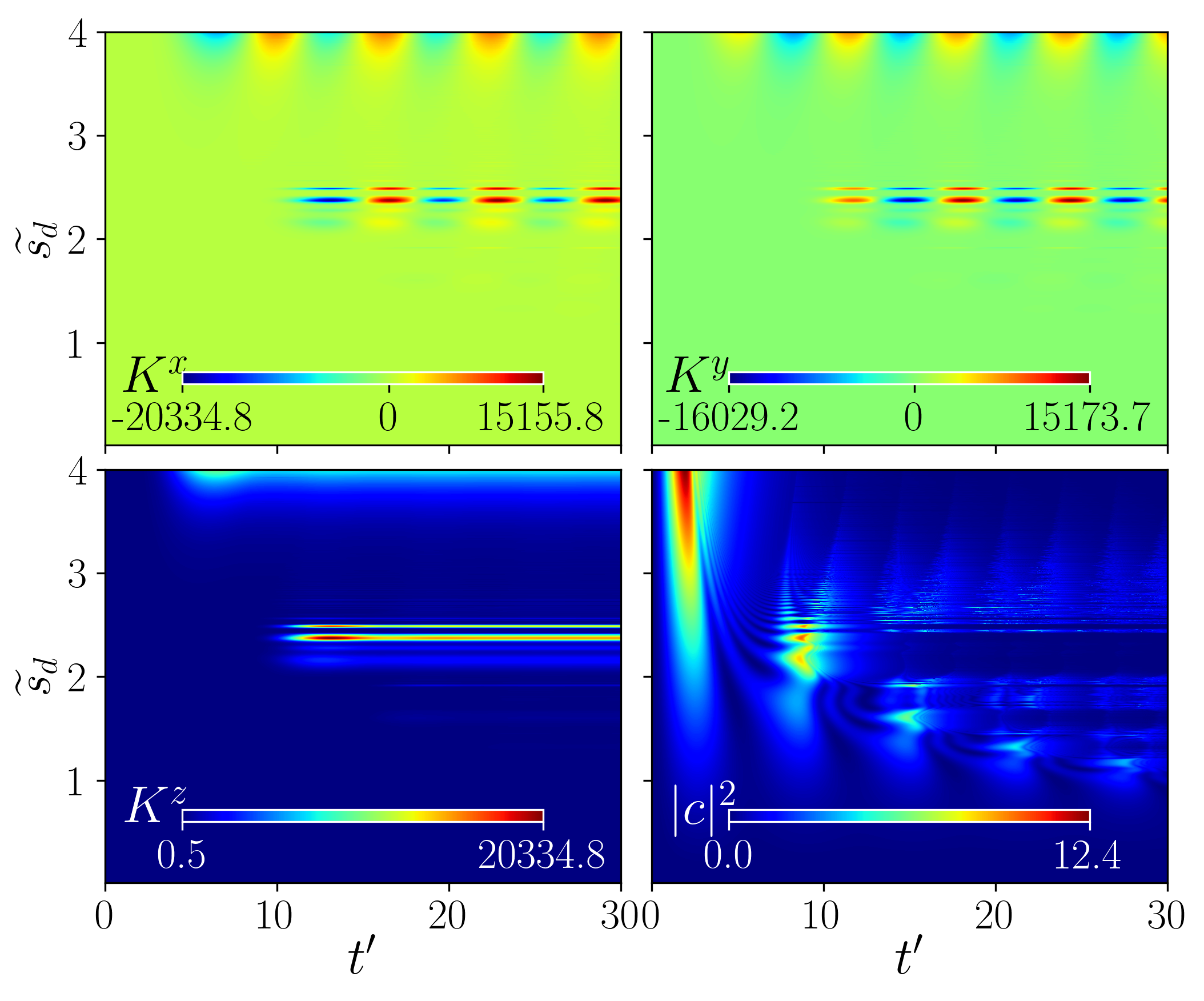
Figure 8: Temporal evaluation of pseudospin components and the photon field under varying drive power, $\tilde{s}_{d}$ for blue-detuning $\Delta^{\prime}=-1$ with parameters as in Fig. 6.

Fig. 6 shows the temporal behavior of the system under varying drive power for the red-detuned regime. At low drive powers (below a threshold of approximately 1.3 in normalized units), the pseudospin vector $\mathbf{K}=(K_{x},K_{y},K_{z})$ exhibits damped oscillations and eventually reaches a stable fixed point for each specific power level (see App. B for more details). This indicates that for each power value, there is a unique combination of $K_{x}$, $K_{y}$, $K_{z}$, and a corresponding photon number ($|c|^{2}$) that the system settles into. In this regime, the amplification of $|c|^{2}$ is power-dependent, reaching its maximum value at the threshold power. However, the behavior changes significantly when the drive power exceeds this threshold. Initially, $|c|^{2}$ increases rapidly, but the backaction by $\mathbf{K}$ on $|c|^{2}$ reduces it to nearly zero (a bit before $t^{\prime}=10$). With the optical cavity being essentially empty, the pseudospin $\mathbf{K}$ precesses at its natural frequency of approximately $2\omega_{m}$. These oscillations persist due to the small intrinsic damping of the magnons. Thus, the optical input excites self-sustained oscillations in the magnon pairs beyond the threshold power.

The system’s dynamics for the resonant ($\Delta^{\prime}=0$) and blue-detuned ($\Delta^{\prime}=-1$) regimes are illustrated in Figs. 7 and 8, respectively. In both cases, stable oscillations are observed when the input power remains below a critical threshold value of 1. Further details on the analysis can be found in App. B. For input powers exceeding this critical value, the system undergoes a transition to a chaotic regime. This transition is attributed to a significant energy transfer to the AFM, manifested by a continuous increase in the $K^{z}$ component over time. This increasing $K^{z}$ signifies the onset of a dynamical instability in the system.

V Conclusion

In summary, we theoretically explored the potential of using high-finesse optical cavities to precisely manipulate and control the dynamics of magnons in AFM insulators, including Rutiles and cuprates. We focused on materials where two-magnon Raman scattering is crucial in coupling the photon cavity with AFM spin sublattices. This mechanism facilitates the generation of pure magnon pairs and induces shifts in the magnon frequency spectrum. We demonstrated that when the drive laser and cavity photons are red-detuned, there exists a certain power threshold for the pump. Below this threshold, magnon-pair squeezing is evident, while above it, magnon pairs transition into a limit cycle. To characterize the features of attractor points and determine stability conditions in the squeezing states, we used the fast cavity approximation.

Within these AFMs, magnons have an intrinsic capability to generate squeezed states due to interference between sublattice spin waves. Using an optical cavity, we can modulate these pre-existing squeezing states for applications in quantum information. Higher squeezing factors suggest the potential for cavity control of AFM magnons, e.g. for controlling the phase diagram of materials where spin fluctuations are believed to play an important role, such as high-T_c cuprate superconductors. Furthermore, squeezing leads to an increased precision in sensing a conjugate variable (here, proportional to the photon number).

The squeezing factor, a key metric of our study, can be experimentally measured using Brillouin light scattering techniques. Employing Eq. (12) and the input-output formalism, the scattered light $\hat{c}_{\rm out}$ can be expressed in terms of the incoming light $\hat{c}_{\rm in}$ and the Perelomov operators as

$$\hat{c}_{\rm out}-\hat{c}_{\rm in}\propto 2\mathcal{R}\hat{K}^{z}+\mathcal{T}\hat{K}^{-}+\mathcal{T}^{*}\hat{K}^{+}\,.$$ (36)

Since the phase of $\mathcal{T}$ depends on the polarization of the incident light, derived via Eq. (6), by measuring both the mean and the fluctuations of the output field, we obtain analogous information for an arbitrary pseudospin component, say $\sum_{i}\xi_{i}\hat{K}^{i}$ for some constants $\xi_{i}$. By systematically varying the values of $\xi_{i}$, one can derive the averages up to the second order in terms of $\hat{K}^{i}$, thereby revealing the squeezing parameter $q^{i}$.

Furthermore, we showed that when the pump and cavity photons are at resonance or blue-detuned, depending on the pump power, magnon-pairs exhibit nonlinear dynamics such as auto-oscillations and chaos. This can open the door to novel spintronic applications, including spin-torque nano-oscillators (STNOs) and magnonic logic devices.

VI Acknowledgement

S.S. and S.V.K. acknowledge funding from the Bundesministerium für Bildung und Forschung (BMBF) under the project QECHQS (Grant No. 16KIS1590K) and the Deutsche Forschungsgemeinschaft (DFG, German Research Foundation)—Project-ID 429529648—TRR 306 QuCoLiMa (“Quantum Cooperativity of Light and Matter”). A.-L.E.R. received the support of a fellowship from the ”la Caixa” Foundation (ID 100010434). The fellowship code is LCF/BQ/DI22/11940029.

Appendix A Antiferromagnetic Hamiltonian

In this appendix, we consider the diagonalization of the AFM Hamiltonian in two distinct categories of AFM insulators. The first class consists of materials with rutile crystal structures, such as MnF₂ and FeF₂. These materials feature a body-centered tetragonal lattice, where magnetic ions reside at the corners and body-centered positions, as depicted in Fig. 9(a). Additionally, they exhibit uniaxial (easy-axis) anisotropy. Below their respective Néel temperatures (66.5 K for MnF₂ and 78.4 K for FeF₂), and in the absence of an external magnetic field, the spins order into two sublattices with opposite orientations along the easy anisotropy direction (c-axis).

The second class of AFM insulators considered in this study comprises cuprate parent compounds, including La₂CuO₄, YBa₂Cu₃O₆, and Tl₂Ba₂CuO₆. These high-$T_{c}$ compounds possess a layered structure composed of intercalated copper-oxygen planes. For simplicity, we disregard interlayer couplings and instead consider quasi-two-dimensional (2D) constituents, as depicted in Fig. 10(a).

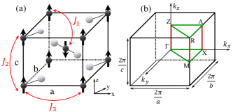
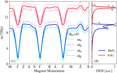
Figure 9: (a) Crystal and magnetic structure of the rutile AFMs MnF₂ and FeF₂. The large circles show the position of Mn²⁺ (or Fe²⁺) ions with their magnetic moment directions shown as arrows. The small circles represent the fluorine atoms. (b) The primitive Brillouin zone, critical points, and symmetric lines of the rutile AFMs. (c) Magnon dispersion for $B_{0}=0$ (solid lines) and $B_{0}=4T$ (dotted and dash-dotted lines) and (d) one-magnon density of states (DOS) in MnF₂ (blue) and FeF₂ (red). $\omega_{\mathrm{M}}^{\mathrm{MnF_{2}}}=9.25$THz and $\omega_{\mathrm{M}}^{\mathrm{FeF_{2}}}=14.55$THz.

In the Heisenberg spin model, the Hamiltonian is given by

$$\hat{\mathcal{H}}_{m}=\sum_{\mathbf{R}}\left[\sum_{\mathbf{R}^{\prime}}J_{\mathbf{R^{\prime}}}\hat{\boldsymbol{S}}_{\mathbf{R}}\cdot\hat{\boldsymbol{S}}_{\mathbf{R}+\mathbf{R}^{\prime}}-D\left(\hat{S}_{\mathbf{R}}^{z}\right)^{2}-B_{0}\hat{S}_{\mathbf{R}}^{z}\right],$$ (37)

where $\hat{\boldsymbol{S}}_{\mathbf{R}}$ denotes a spin-$S$ particle located at site $\mathbf{R}$, $J_{\mathbf{R}^{\prime}}$ is the exchange interaction between spins displaced by $\mathbf{R}^{\prime}$, and $B_{0}$ is an external magnetic field.

We consider up to the third-nearest neighbor with exchange constants $J_{1}$, $J_{2}$, and $J_{3}$. The number of neighbors corresponding to each exchange is $z_{1}=8$, $z_{2}=2$, and $z_{3}=4$ for Rutile-AFMs and $z_{1}=z_{2}=z_{3}=4$ for cuprates. The second term in the Hamiltonian represents the easy-axis anisotropy term, which is related to the anisotropy field $H_{A}$ through the equation $D=g\mu_{B}H_{A}/(2S)$, where $g$ represents the spectroscopic splitting factor, and $\mu_{B}$ is the Bohr magneton. This uniaxial anisotropy aligns the Néel vector in the $\mathbf{z}$ direction.

The low-energy excitations of $\hat{\mathcal{H}}_{0}$ to the lowest order in $1/S$ are found by Holstein-Primakoff linear spin-wave theory. Transforming to Fourier space the Hamiltonian can be recast as $\hat{\mathcal{H}}_{0}=\sum_{{\bf k}}\psi_{{\bf k}}^{\dagger}\mathcal{H}_{{\bf k}}\psi_{{\bf k}}$ in the Nambu basis $\psi_{\bf{k}}^{\dagger}=(a_{\mathbf{k}}^{\dagger},b_{-{\bf k}})$. $\mathcal{H}_{{\bf k}}=h_{0}I+h_{x}\sigma_{x}+h_{z}\sigma_{z}$ where $\sigma$ is the vector of Pauli matrices and $h_{0}=J_{{\bf k}}+2SD$, $h_{x}=z_{1}SJ_{1}\gamma_{1{\bf k}}$, $h_{z}=g\mu_{B}B_{0}$, with $J_{{\bf k}}=z_{1}SJ_{1}+z_{2}SJ_{2}\left(\gamma_{2\mathbf{k}}-1\right)+z_{3}SJ_{3}\left(\gamma_{3\mathbf{k}}-1\right)$, and geometric structure factors

$$\gamma_{\bf{1k}} =\cos(ak_{x}/2)\cos(bk_{y}/2)\cos(ck_{z}/2),$$

$$\gamma_{\bf{2k}} =\cos\left(k_{z}c\right),$$

$$\gamma_{3\bf{k}} =[\cos(ak_{x})+\cos(bk_{y})]/2,$$ (38)

The lattice constants are $a=b=$4.874\text{\,}\mathrm{\SIUnitSymbolAngstrom}$$ and $c=$3.31\text{\,}\mathrm{\SIUnitSymbolAngstrom}$$ for MnF₂ and $a=b=$4.697\text{\,}\mathrm{\SIUnitSymbolAngstrom}$$ and $c=$3.309\text{\,}\mathrm{\SIUnitSymbolAngstrom}$$ for FeF₂ Hutchings et al. (1970); Rezende (1978); Ohlmann and Tinkham (1961). The unperturbed Hamiltonian is diagonalized to $\hat{\mathcal{H}}_{0}=E_{0}+\sum_{{\bf k}}\left[\varepsilon_{\alpha{\bf k}}\alpha_{{\bf k}}^{\dagger}\alpha_{{\bf k}}+\varepsilon_{\beta{\bf k}}\beta_{-{\bf k}}^{\dagger}\beta_{-{\bf k}}\right]$ via Bogoliubov transformation Rezende et al. (2019); Parvini et al. (2020); Boström et al. (2021)

$$\begin{pmatrix}a_{\mathbf{k}}\\ b_{\mathbf{-k}}^{\dagger}\end{pmatrix}=\begin{pmatrix}\cosh(\theta_{\bf k}/2)&-\sinh(\theta_{\bf k}/2)\\ -\sinh(\theta_{\bf k}/2)&\cosh(\theta_{\bf k}/2)\end{pmatrix}\begin{pmatrix}\alpha_{\mathbf{k}}\\ \beta_{\mathbf{-k}}^{\dagger}\end{pmatrix},$$ (39)

the Bogoliubov angle is $\theta_{{\bf k}}=\tanh^{-1}\left(h_{x}/h_{0}\right)$, and the dispersion of the upper and lower magnon branches is $\varepsilon_{\alpha/\beta}=\pm h_{z}+\sqrt{h_{0}^{2}-h_{x}^{2}}$. Only at ${\bf k}=0$, the dispersion terms associated with $J_{2}$ and $J_{3}$ vanish. Consequently, retaining these two terms in the Hamiltonian is crucial to study two-magnon Raman scattering, where any type of wavevector can be excited. Table LABEL:table_I lists the exchange constants, spin values, and uniaxial anisotropy constants of FeF₂ and MnF₂. The dipolar interaction mainly governs the magnetic anisotropy in MnF₂, whereas in FeF₂ it arises mainly from spin-orbit coupling and exhibits a substantial magnitude. Similarly, the experimental critical temperature $T_{c}$ (K) and the calculated exchange interactions (meV) for these quasi 2D cuprates are presented in Table LABEL:table:MO_coeff.

The magnon dispersion curves and density of states (DOS) for MnF₂ and FeF₂ are shown in Fig. 9. The magnon modes exhibit degeneracy (solid lines) in the absence of an external magnetic field. The higher-frequency peak corresponds to magnons near the Brillouin zone’s end faces along the z-direction. At $B_{0}=0$, the frequency of the $\Gamma$-magnon in MnF₂ is $1.64\text{\,}\mathrm{THz}$. As the wave number increases, the frequency increases owing to higher exchange energies, eventually reaching nearly $10\text{\,}\mathrm{THz}$ at the zone boundary. In contrast, FeF₂ exhibits a substantially higher predicted frequency of $10\text{\,}\mathrm{THz}$ for the $\Gamma$-magnon, mainly because of its significant anisotropy. At the zone boundary, the frequency value is projected to further amplify to approximately $15\text{\,}\mathrm{THz}$. The effect of the magnetic field on dispersion in FeF₂ is negligible, as shown in Fig. 9, and is completely absent in $\omega_{\alpha}+\omega_{\beta}$ due to the neglected orthorhombic anisotropy. In addition, the density of magnon states shows prominent peaks near the van Hove singularities, which are located close to the Brillouin zone boundary.

Table 1: spin value, g-factor, exchange constants, and uniaxial anisotropy fields (meV) associated with Rutile AFMs Nikotin et al. (1969); Hutchings et al. (1970).

AFM				S			g			$J_{1}$			$J_{2}$			$J_{3}$			$g\mu_{B}B_{A}$
MnF2				5/2			2			0.304			-0.056			0.008			0.095
FeF2				2			2.22			0.45			-0.0062			0.024			2.57

Table 2: Experimental critical temperature T_c(K), exchange constants (meV), and lattice constant $a$ (Å) for parent cuprates-AFMs Wan et al. (2009); Tam et al. (2022); Keimer et al. (1992); Armstrong (2010); Canali and Girvin (1992); Sandvik et al. (1998).

cuprates-AFM				$J_{1}$			$J_{2}$			$J_{3}$			$T_{c}$			a
La2CuO4				108.8			-12.0			-0.2			42			3.81
YBa2Cu3O6				93.0			-4.7			2.4			90			3.85

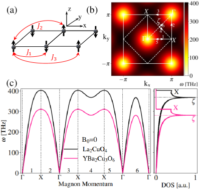
Figure 10: (a) Magnetic structure and definition of short-range exchange constants $J_{l}$ ($l=1,2,3$) up to the third nearest-neighbor (NNN) for two-dimensional cuprates, (b) Magnon dispersion and first Brillouin zone in La₂CuO₄, (c) Magnon dispersion and density of states for monolayers of La₂CuO₄ and YBa₂Cu₃O₆.

For spin-up and spin-down modes, the X-point of the energy spectrum is a local maximum, and the midpoint between X points is a saddle point, as shown in Fig. 10(c). This feature gives rise to Van Hove singularity in the magnon DOS, $\zeta$ point. Compared with rutile AFMs, Fig. 9, the magnon modes in these materials have a higher frequency.

Appendix B Full-Dynamic Response of Optomagnonic Cavity

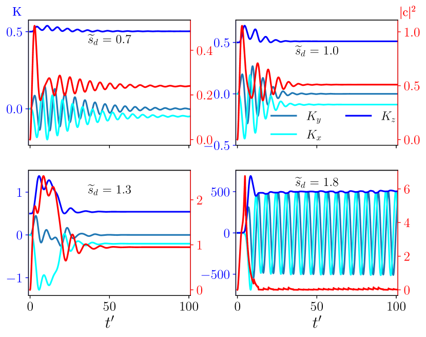
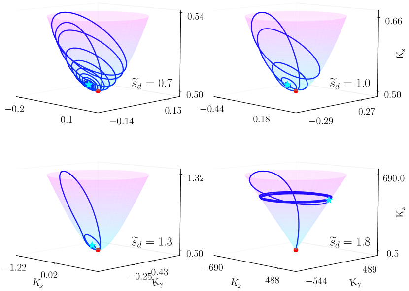
Figure 11: Temporal evolution of pseudospin components $K_{x}$, $K_{y}$ and $K_{z}$ and the photon field under varying normalized derive laser power. $\Delta^{\prime}=1$, $\kappa_{G}^{\prime}=10^{-4}$, and initial pseudospin state ${\bf K}_{0}=\frac{1}{2}[0,0,1]$ and $c(0)=0$.

Fig. 11 shows the temporal evolution of the pseudospin components ($K^{x}$, $K^{y}$, and $K^{z}$) and the photon field under varying driving laser power for a specific case: a photon cavity and drive laser detuning of $\Delta^{\prime}=1$. The figure also presents the corresponding trajectories of the pseudospin tip on the upper hyperboloid sheet. The short simulation time ($t^{\prime}=100$) allows for a detailed observation of the dynamic behavior. The numerical simulations reveal a distinct power threshold for the driving laser, identified at approximately 1.3. Below this threshold, the pseudospin components converge towards a stable equilibrium point (attractor). However, beyond this critical value, the pseudospin dynamics transition into a sustained oscillatory regime. In this regime, $K^{z}$ reaches a constant value, while the photon field decays to zero amplitude. Notably, within the damped oscillator regime (below the threshold), the phase difference between the magnon creation and annihilation operators stabilizes at $2\pi$ after reaching the attractor point. Conversely, in the oscillatory state (above the threshold), this phase difference exhibits dynamic fluctuations within the range of $-2\pi$ to $2\pi$, as shown in Fig. 12.

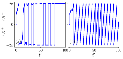
Figure 12: Phase difference between magnon creation and annihilation operators for (a) $\tilde{s}_{d}=1.3$ and (b) $\tilde{s}_{d}=1.8$.

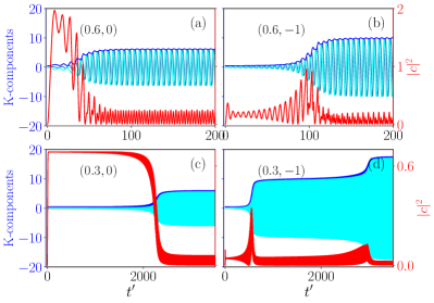
Figure 13: Temporal evolution of pseudospin components $K_{x}$, $K_{y}$, and $K_{z}$, along with the photon field, for varying pairs of parameters $(\tilde{s}_{d},\Delta^{\prime})$.

The temporal evolution of the pseudospin and photon field for $\Delta^{\prime}=0$ ($\omega_{d}=\omega_{c}$) and $\Delta^{\prime}=-1$ ($\omega_{d}>\omega_{c}$) are shown in Fig. 13. The results show the emergence of auto-oscillation states with varying amplitudes and frequencies depending on the pump laser power. These auto-oscillatory behaviors hold promise for applications in modern spin-torque oscillators (STTNOs), signal processing, and other related fields  Sadat Parvini et al. (2023); Urazhdin et al. (2010).

Appendix C Squeezing of Perelomov Coherent States

This section discusses the basic mathematical results of the Perelomov coherent states that help derive various averages in the main text. For a fixed pseudo-spin $K$, they are defined by $\Ket{K,\vartheta,\varphi}=\hat{\cal D}(\vartheta,\varphi)\Ket{0,K}$ where $\hat{\cal D}=\exp(-\vartheta\hat{A})$ with

$$\hat{A}=\frac{-e^{-i\varphi}\hat{K}^{+}+e^{i\varphi}\hat{K}^{-}}{2}.$$ (40)

For later convenience, we also define

$$\hat{B}=\frac{e^{-i\varphi}\hat{K}^{+}+e^{i\varphi}\hat{K}^{-}}{2}.$$ (41)

We have the commutation relations $\left[\hat{A},\hat{K}^{z}\right]=\hat{B}$, $\left[\hat{B},\hat{K}^{z}\right]=\hat{A}$, and $\left[\hat{A},\hat{B}\right]=\hat{K}^{z}$. Below, we will use the Baker-Campbell-Hausdorff (BCH) formula

$$e^{\hat{X}}\hat{Y}e^{-\hat{X}}=\hat{Y}+\frac{[\hat{X},\hat{Y}]}{1!}+\frac{[\hat{X},[\hat{X},\hat{Y}]]}{2!}+\dots$$ (42)

We now find how the operators $\{\hat{A},\hat{B},\hat{K}^{z}\}$ transform under $\hat{\cal D}$. We already know that $\hat{\cal D}^{\dagger}\hat{A}\hat{\cal D}=\hat{A}$ because $\hat{A}$ commutes with $\hat{\cal D}$. We can find $\hat{\cal D}^{\dagger}\hat{B}\hat{\cal D}$ using the BCH formula and the commutation relations written above,

$$\hat{\cal D}^{\dagger}\hat{B}\hat{\cal D}=\cosh\vartheta\hat{B}+\sinh\vartheta\hat{K}^{z}.$$ (43)

Similarly, we can derive

$$\hat{\cal D}^{\dagger}\hat{K}^{z}\hat{\cal D}=\sinh\vartheta\hat{B}+\cosh\vartheta\hat{K}^{z}.$$ (44)

Now, we know the averages in the ground state as $\langle\hat{K}^{z}\rangle_{0}=K$ and $\langle\hat{K}^{\pm}\rangle_{0}=0$ where $\langle\hat{X}\rangle_{0}=\Braket{K,0}{\hat{X}}{K,0}$. The averages in the Perelomov coherent states, defined as $\langle\hat{X}\rangle=\Braket{K,\vartheta,\varphi}{\hat{X}}{K,\vartheta,\varphi}$, can be found using the above transformations: $\langle\hat{K}^{z}\rangle=K\cosh\vartheta$, $\langle\hat{A}\rangle=0$ and $\langle\hat{B}\rangle=K\sinh\vartheta$. The last two expressions also imply $\langle\hat{K}^{\pm}\rangle=Ke^{\pm i\varphi}\sinh\vartheta$. A useful relation derived from the above is

$$\hat{\cal D}^{\dagger}\left(\hat{K}^{-}-e^{-i\varphi}\tanh\frac{\vartheta}{2}\hat{K}^{z}\right)\hat{\cal D}=\hat{K}^{-}+e^{-i\varphi}\hat{K}^{z}\tanh\frac{\vartheta}{2}.$$ (45)

Using $\hat{K}^{z}\Ket{K,0}=K\Ket{K,0}$ and $\hat{K}^{-}\Ket{K,0}=0$, this gives the effect of $\hat{K}^{-}$ on coherent states as $\hat{K}^{-}\Ket{K,\vartheta,\varphi}=\lambda\left(K+\hat{K}^{z}\right)\Ket{K,\vartheta,\varphi}$ where $\lambda=e^{-i\varphi}\tanh\frac{\vartheta}{2}$.

To calculate the squeezing parameters, we want to find variances of $\hat{K}^{x}$ and $\hat{K}^{y}$. To this end, we again use the transformations

$$\left\langle\hat{A}^{2}\right\rangle=\left\langle\hat{A}^{2}\right\rangle_{0}=\frac{-K}{2},$$ (46)

where we used $\hat{K}^{-}\hat{K}^{+}\Ket{K,0}=2K\Ket{K,0}$. Similarly,

$$\left\langle\hat{B}^{2}\right\rangle=\frac{K}{2}\cosh^{2}\vartheta+K^{2}\sinh^{2}\vartheta,$$ (47)

and the cross-correlation

$$\left\langle\hat{A}\hat{B}\right\rangle=\frac{K}{2}\cosh\vartheta.$$ (48)

Using $\hat{K}^{x}=\hat{B}\cos\varphi-i\hat{A}\sin\varphi$, we find the variance

$$\left\langle\left(\Delta\hat{K}^{x}\right)^{2}\right\rangle=\frac{K}{2}\left(1+\sinh^{2}\vartheta\cos^{2}\varphi\right)$$ (49)

and similar result holds with $\hat{K}^{x}\rightarrow\hat{K}^{y}$ and $\cos\varphi\rightarrow\sin\varphi$. These calculations and formulations lay the groundwork for exploring squeezing phenomena in this paper.

References

- KEYES (1981) R. KEYES, in VLSI Electronics: Microstructure Science, Vol. 1, edited by N. G. Einspruch (Elsevier, 1981) pp. 185–230.
- Vashchenko and Sinkevitch (2008) V. A. Vashchenko and V. F. Sinkevitch, Physical limitations of semiconductor devices, Vol. 340 (Springer, 2008).
- Keyes (2001) R. W. Keyes, Proc. IEEE 89, 227 (2001).
- Flebus et al. (2024) B. Flebus, D. Grundler, B. Rana, Y. Otani, I. Barsukov, A. Barman, G. Gubbiotti, P. Landeros, J. Akerman, U. Ebels, P. Pirro, V. E. Demidov, K. Schultheiss, G. Csaba, Q. Wang, F. Ciubotaru, D. E. Nikonov, P. Che, R. Hertel, T. Ono, D. Afanasiev, J. Mentink, T. Rasing, B. Hillebrands, S. V. Kusminskiy, W. Zhang, C. R. Du, A. Finco, T. van der Sar, Y. K. Luo, Y. Shiota, J. Sklenar, T. Yu, and J. Rao, J. Phys. Condens. Matter 36, 363501 (2024).
- Chumak et al. (2022) A. V. Chumak, P. Kabos, M. Wu, C. Abert, C. Adelmann, A. O. Adeyeye, J. Åkerman, F. G. Aliev, A. Anane, A. Awad, C. H. Back, A. Barman, G. E. W. Bauer, M. Becherer, E. N. Beginin, V. A. S. V. Bittencourt, Y. M. Blanter, P. Bortolotti, I. Boventer, D. A. Bozhko, S. A. Bunyaev, J. J. Carmiggelt, R. R. Cheenikundil, F. Ciubotaru, S. Cotofana, G. Csaba, O. V. Dobrovolskiy, C. Dubs, M. Elyasi, K. G. Fripp, H. Fulara, I. A. Golovchanskiy, C. Gonzalez-Ballestero, P. Graczyk, D. Grundler, P. Gruszecki, G. Gubbiotti, K. Guslienko, A. Haldar, S. Hamdioui, R. Hertel, B. Hillebrands, T. Hioki, A. Houshang, C.-M. Hu, H. Huebl, M. Huth, E. Iacocca, M. B. Jungfleisch, G. N. Kakazei, A. Khitun, R. Khymyn, T. Kikkawa, M. Kläui, O. Klein, J. W. Kłos, S. Knauer, S. Koraltan, M. Kostylev, M. Krawczyk, I. N. Krivorotov, V. V. Kruglyak, D. Lachance-Quirion, S. Ladak, R. Lebrun, Y. Li, M. Lindner, R. Macêdo, S. Mayr, G. A. Melkov, S. Mieszczak, Y. Nakamura, H. T. Nembach, A. A. Nikitin, S. A. Nikitov, V. Novosad, J. A. Otálora, Y. Otani, A. Papp, B. Pigeau, P. Pirro, W. Porod, F. Porrati, H. Qin, B. Rana, T. Reimann, F. Riente, O. Romero-Isart, A. Ross, A. V. Sadovnikov, A. R. Safin, E. Saitoh, G. Schmidt, H. Schultheiss, K. Schultheiss, A. A. Serga, S. Sharma, J. M. Shaw, D. Suess, O. Surzhenko, K. Szulc, T. Taniguchi, M. Urbánek, K. Usami, A. B. Ustinov, T. van der Sar, S. van Dijken, V. I. Vasyuchka, R. Verba, S. Viola Kusminskiy, Q. Wang, M. Weides, M. Weiler, S. Wintz, S. P. Wolski, and X. Zhang, IEEE Trans. Magn. 58, 1 (2022).
- Baltz et al. (2018) V. Baltz, A. Manchon, M. Tsoi, T. Moriyama, T. Ono, and Y. Tserkovnyak, Rev. Mod. Phys. 90, 015005 (2018).
- Jungwirth et al. (2018) T. Jungwirth, J. Sinova, A. Manchon, X. Marti, J. Wunderlich, and C. Felser, Nat. Phys. 14, 200 (2018).
- Spaldin (2010) N. A. Spaldin, Magnetic materials: fundamentals and applications (Cambridge university press, 2010).
- Duine et al. (2018) R. Duine, K.-J. Lee, S. S. Parkin, and M. D. Stiles, Nat. Phys. 14, 217 (2018).
- Han et al. (2023) J. Han, R. Cheng, L. Liu, H. Ohno, and S. Fukami, Nat. Mater. 22, 684 (2023).
- Jungwirth et al. (2016) T. Jungwirth, X. Marti, P. Wadley, and J. Wunderlich, Nat. Nanotechnol. 11, 231 (2016).
- Qaiumzadeh et al. (2018) A. Qaiumzadeh, I. A. Ado, R. A. Duine, M. Titov, and A. Brataas, Phys. Rev. Lett. 120, 197202 (2018).
- Chumak et al. (2015) A. V. Chumak, V. I. Vasyuchka, A. A. Serga, and B. Hillebrands, Nat. Phys. 11, 453 (2015).
- Chumak (2019) A. V. Chumak, in Spintronics Handbook, Second Edition: Spin Transport and Magnetism (CRC Press, 2019) pp. 247–302.
- Wang et al. (2020) Q. Wang, M. Kewenig, M. Schneider, R. Verba, F. Kohl, B. Heinz, M. Geilen, M. Mohseni, B. Lägel, F. Ciubotaru, et al., Nat. Electron. 3, 765 (2020).
- Hortensius et al. (2021) J. Hortensius, D. Afanasiev, M. Matthiesen, R. Leenders, R. Citro, A. Kimel, R. Mikhaylovskiy, B. Ivanov, and A. Caviglia, Nat. Phys. 17, 1001 (2021).
- Borovik-Romanov and Kreines (1982) A. Borovik-Romanov and N. Kreines, Phys. Rep. 81, 351 (1982).
- Železnỳ et al. (2014) J. Železnỳ, H. Gao, K. Vỳbornỳ, J. Zemen, J. Mašek, A. Manchon, J. Wunderlich, J. Sinova, and T. Jungwirth, Phys. Rev. Lett. 113, 157201 (2014).
- Wadley et al. (2016) P. Wadley, B. Howells, J. Železnỳ, C. Andrews, V. Hills, R. P. Campion, V. Novák, K. Olejník, F. Maccherozzi, S. Dhesi, et al., Science 351, 587 (2016).
- Moriyama et al. (2018) T. Moriyama, K. Oda, T. Ohkochi, M. Kimata, and T. Ono, Scientific reports 8, 14167 (2018).
- Wienholdt et al. (2012) S. Wienholdt, D. Hinzke, and U. Nowak, Phys. Rev. Lett. 108, 247207 (2012).
- Bossini et al. (2019) D. Bossini, S. Dal Conte, G. Cerullo, O. Gomonay, R. Pisarev, M. Borovsak, D. Mihailovic, J. Sinova, J. Mentink, T. Rasing, et al., Phys. Rev. B 100, 024428 (2019).
- Olejník et al. (2018) K. Olejník, T. Seifert, Z. Kašpar, V. Novák, P. Wadley, R. P. Campion, M. Baumgartner, P. Gambardella, P. Němec, J. Wunderlich, et al., Sci. Adv. 4, eaar3566 (2018).
- Satoh et al. (2015) T. Satoh, R. Iida, T. Higuchi, M. Fiebig, and T. Shimura, Nat. Photonics 9, 25 (2015).
- Kimel et al. (2024) A. Kimel, T. Rasing, and B. Ivanov, J. Magn. Magn. Mater. 598, 172039 (2024).
- Němec et al. (2018) P. Němec, M. Fiebig, T. Kampfrath, and A. V. Kimel, Nat. Phys. 14, 229 (2018).
- Surynek et al. (2024) M. Surynek, J. Zubac, K. Olejnik, A. Farkas, F. Krizek, L. Nadvornik, P. Kubascik, F. Trojanek, R. Campion, V. Novak, et al., arXiv preprint arXiv:2401.17370 (2024).
- Viola Kusminskiy (2019) S. Viola Kusminskiy, Quantum Magnetism, Spin Waves, and Optical Cavities (Springer Cham, 2019).
- Almpanis (2021) E. Almpanis, Optomagnonic Structures: Novel Architectures for Simultaneous Control of Light and Spin Waves (World Scientific, 2021).
- Rameshti et al. (2022) B. Z. Rameshti, S. Viola Kusminskiy, J. A. Haigh, K. Usami, D. Lachance-Quirion, Y. Nakamura, C.-M. Hu, H. X. Tang, G. E. Bauer, and Y. M. Blanter, Phys. Rep. 979, 1 (2022).
- Lee et al. (2023) J. M. Lee, H.-W. Lee, and M.-J. Hwang, Phys. Rev. B 108, L241404 (2023).
- Sharma et al. (2022) S. Sharma, V. A. Bittencourt, and S. Viola Kusminskiy, Journal of Physics: Materials 5, 034006 (2022).
- Zhang et al. (2014) X. Zhang, C.-L. Zou, L. Jiang, and H. X. Tang, Phys. Rev. Lett. 113, 156401 (2014).
- Hisatomi et al. (2016) R. Hisatomi, A. Osada, Y. Tabuchi, T. Ishikawa, A. Noguchi, R. Yamazaki, K. Usami, and Y. Nakamura, Phys. Rev. B 93, 174427 (2016).
- Viola Kusminskiy et al. (2016) S. Viola Kusminskiy, H. X. Tang, and F. Marquardt, Phys. Rev. A 94, 033821 (2016).
- Liu et al. (2016) T. Liu, X. Zhang, H. X. Tang, and M. E. Flatté, Phys. Rev. B 94, 060405 (2016).
- Osada et al. (2018) A. Osada, A. Gloppe, R. Hisatomi, A. Noguchi, R. Yamazaki, M. Nomura, Y. Nakamura, and K. Usami, Phys. Rev. Lett. 120, 133602 (2018).
- Liang et al. (2023) Z. Liang, J. Li, and Y. Wu, Phys. Rev. A 107, 033701 (2023).
- Sharma et al. (2019) S. Sharma, B. Z. Rameshti, Y. M. Blanter, and G. E. Bauer, Phys. Rev. B 99, 214423 (2019).
- Haigh et al. (2016) J. Haigh, A. Nunnenkamp, A. Ramsay, and A. Ferguson, Phys. Rev. Lett. 117, 133602 (2016).
- Šimić et al. (2020) F. Šimić, S. Sharma, Y. M. Blanter, and G. E. W. Bauer, Phys. Rev. B 101, 100401 (2020).
- Sharma et al. (2024) S. Sharma, S. Viola Kusminskiy, and V. A. S. V. Bittencourt, Phys. Rev. B 110, 014416 (2024).
- Parvini et al. (2020) T. S. Parvini, V. A. Bittencourt, and S. Viola Kusminskiy, Phys. Rev. Res. 2, 022027 (2020).
- Xiao et al. (2019) Y. Xiao, X. Yan, Y. Zhang, V. Grigoryan, C. Hu, H. Guo, and K. Xia, Phys. Rev. B 99, 094407 (2019).
- Curtis et al. (2022) J. B. Curtis, A. Grankin, N. R. Poniatowski, V. M. Galitski, P. Narang, and E. Demler, Phys. Rev. Res. 4, 013101 (2022).
- Boventer et al. (2023) I. Boventer, H. Simensen, B. Brekke, M. Weides, A. Anane, M. Kläui, A. Brataas, and R. Lebrun, Phys. Rev. Appl. 19, 014071 (2023).
- Białek et al. (2021) M. Białek, J. Zhang, H. Yu, and J.-P. Ansermet, Phys. Rev. Appl. 15, 044018 (2021).
- Zhang et al. (2021a) Q. Zhang, Y. Sun, Z. Lu, J. Guo, J. Xue, Y. Chen, Y. Tian, S. Yan, and L. Bai, Appl. Phys. Lett. 119 (2021a).
- Fleury and Loudon (1968) P. A. Fleury and R. Loudon, Phys. Rev. 166, 514 (1968).
- Fleury et al. (1966) P. Fleury, S. Porto, L. Cheesman, and H. Guggenheim, Phys. Rev. Lett. 17, 84 (1966).
- Loudon (1968) R. Loudon, Adv. Phys. 17, 243 (1968).
- Fleury et al. (1967) P. A. Fleury, S. P. S. Porto, and R. Loudon, Phys. Rev. Lett. 18, 658 (1967).
- Lockwood and Cottam (1987) D. J. Lockwood and M. G. Cottam, Phys. Rev. B 35, 1973 (1987).
- Cottam et al. (1983) M. Cottam, V. So, D. Lockwood, R. Katiyar, and H. Guggenheim, J. phys., C, Solid state phys. 16, 1741 (1983).
- Lee et al. (2006) P. A. Lee, N. Nagaosa, and X.-G. Wen, Rev. Mod. Phys. 78, 17 (2006).
- Moriya and Ueda (2003) T. Moriya and K. Ueda, Rep. Prog. Phys. 66, 1299 (2003).
- Erlandsen et al. (2019) E. Erlandsen, A. Kamra, A. Brataas, and A. Sudbø, Phys. Rev. B 100, 100503 (2019).
- Canali and Girvin (1992) C. Canali and S. Girvin, Phys. Rev. B 45, 7127 (1992).
- Kastner et al. (1998) M. Kastner, R. Birgeneau, G. Shirane, and Y. Endoh, Rev. Mod. Phys. 70, 897 (1998).
- Betto et al. (2021) D. Betto, R. Fumagalli, L. Martinelli, M. Rossi, R. Piombo, K. Yoshimi, D. Di Castro, E. Di Gennaro, A. Sambri, D. Bonn, et al., Phys. Rev. B 103, L140409 (2021).
- Scalapino (2012) D. J. Scalapino, Rev. Mod. Phys. 84, 1383 (2012).
- Mitrano et al. (2016) M. Mitrano, A. Cantaluppi, D. Nicoletti, S. Kaiser, A. Perucchi, S. Lupi, P. Di Pietro, D. Pontiroli, M. Riccò, S. R. Clark, et al., Nature 530, 461 (2016).
- Mankowsky et al. (2014) R. Mankowsky, A. Subedi, M. Först, S. O. Mariager, M. Chollet, H. Lemke, J. S. Robinson, J. M. Glownia, M. P. Minitti, A. Frano, et al., Nature 516, 71 (2014).
- Odagaki and Tani (1971) T. Odagaki and K. Tani, Phys. Lett. A 36, 399 (1971).
- Fedianin et al. (2023) A. E. Fedianin, A. M. Kalashnikova, and J. H. Mentink, Phys. Rev. B 107, 144430 (2023).
- Zhao et al. (2004) J. Zhao, A. V. Bragas, D. J. Lockwood, and R. Merlin, Phys. Rev. Lett. 93, 107203 (2004).
- Hu and Nori (1996a) X. Hu and F. Nori, Phys. Rev. B 53, 2419 (1996a).
- Hu and Nori (1996b) X. Hu and F. Nori, Phys. Rev. Lett. 76, 2294 (1996b).
- Aspelmeyer et al. (2014) M. Aspelmeyer, T. J. Kippenberg, and F. Marquardt, Rev. Mod. Phys. 86, 1391 (2014).
- Perelomov (1975) A. Perelomov, Commun. Math. Phys. 44, 197 (1975).
- Kastrup (2007) H. Kastrup, Annalen der Physik 16, 439 (2007).
- Novaes (2004) M. Novaes, Revista Brasileira de Ensino de Fisica 26, 351 (2004).
- Aravind (1988) P. K. Aravind, J. Opt. Soc. Am. B 5, 1545 (1988).
- Gerry (1985) C. C. Gerry, Phys. Rev. A 31, 2721 (1985).
- Mayergoyz et al. (2009) I. D. Mayergoyz, G. Bertotti, and C. Serpico, Nonlinear magnetization dynamics in nanosystems (Elsevier, 2009).
- Elyasi et al. (2020) M. Elyasi, Y. M. Blanter, and G. E. Bauer, Phys. Rev. B 101, 054402 (2020).
- Rezende and de Aguiar (1990) S. M. Rezende and F. M. de Aguiar, Proc. IEEE 78, 893 (1990).
- Yuan et al. (2022) H. Yuan, Y. Cao, A. Kamra, R. A. Duine, and P. Yan, Phys. Rep. 965, 1 (2022).
- Coldea et al. (2001) R. Coldea, S. Hayden, G. Aeppli, T. Perring, C. Frost, T. Mason, S.-W. Cheong, and Z. Fisk, Phys. Rev. Lett. 86, 5377 (2001).
- Bonesteel (1993) N. Bonesteel, Phys. Rev. B 47, 11302 (1993).
- Chen et al. (2011) W. Chen, O. P. Sushkov, and T. Tohyama, Phys. Rev. B 84, 195125 (2011).
- Govind et al. (2001) Govind, A. Pratap, Ajay, and R. Tripathi, Eur. Phys. J. B 23, 153 (2001).
- Dalla Piazza (2016) B. Dalla Piazza, Excitation Spectra of Square Lattice Antiferromagnets: Theoretical Explanation of Experimental Observations (Springer, 2016).
- Wan et al. (2009) X. Wan, T. A. Maier, and S. Y. Savrasov, Phys. Rev. B 79, 155114 (2009).
- Sandvik et al. (1998) A. W. Sandvik, S. Capponi, D. Poilblanc, and E. Dagotto, Phys. Rev. B 57, 8478 (1998).
- Manousakis (1991) E. Manousakis, Rev. Mod. Phys. 63, 1 (1991).
- Chakravarty et al. (1989) S. Chakravarty, B. I. Halperin, and D. R. Nelson, Phys. Rev. B 39, 2344 (1989).
- Holstein and Primakoff (1940) T. Holstein and H. Primakoff, Phys. Rev. 58, 1098 (1940).
- Cottam (1975) M. Cottam, J. Phys. C: Solid State Phys. 8, 1933 (1975).
- Cottam and Lockwood (1986) M. G. Cottam and D. J. Lockwood, Light scattering in magnetic solids (Wiley, 1986).
- Moriya (1967) T. Moriya, J. Phys. Soc. Jpn. 23, 490 (1967).
- Boström et al. (2023) E. V. Boström, T. S. Parvini, J. W. McIver, A. Rubio, S. Viola Kusminskiy, and M. A. Sentef, Phys. Rev. Lett. 130, 026701 (2023).
- Lockwood and Cottam (2012) D. Lockwood and M. Cottam, Low Temp. Phys. 38, 549 (2012).
- Odagaki (1973a) T. Odagaki, J. Phys. Soc. Jpn. 35, 40 (1973a).
- Odagaki (1973b) T. Odagaki, J. Phys. Soc. Jpn. 35, 1343 (1973b).
- Formisano et al. (2024) F. Formisano, T. Gareev, D. Khusyainov, A. Fedianin, R. Dubrovin, P. Syrnikov, D. Afanasiev, R. Pisarev, A. Kalashnikova, J. Mentink, et al., APL Mater. 12 (2024), 10.1063/5.0180888.
- Dimmock and Wheeler (1962) J. O. Dimmock and R. Wheeler, Phys. Rev. 127, 391 (1962).
- Sugano and Kojima (2013) S. Sugano and N. Kojima, Magneto-optics, Vol. 128 (Springer Science & Business Media, 2013).
- Fleury and Guggenheim (1970) P. Fleury and H. Guggenheim, Phys. Rev. Lett. 24, 1346 (1970).
- Amer et al. (1975) N. M. Amer, T.-c. Chiang, and Y. Shen, Phys. Rev. Lett. 34, 1454 (1975).
- Weber and Merlin (2000) W. H. Weber and R. Merlin, Raman scattering in materials science, Vol. 42 (Springer Science & Business Media, 2000).
- Devereaux and Hackl (2007) T. P. Devereaux and R. Hackl, Rev. Mod. Phys. 79, 175 (2007).
- Poppinger (1977) M. Poppinger, Zeitschrift für Physik B Condensed Matter 27, 61 (1977).
- Davies et al. (1971) R. Davies, S. Chinn, and H. Zeiger, Phys. Rev. B 4, 992 (1971).
- Vernay et al. (2007) F. Vernay, M. Gingras, and T. Devereaux, Phys. Rev. B 75, 020403 (2007).
- Chubukov and Frenkel (1995) A. V. Chubukov and D. M. Frenkel, Phys. Rev. B 52, 9760 (1995).
- Shastry and Shraiman (1990) B. S. Shastry and B. I. Shraiman, Phys. Rev. Lett. 65, 1068 (1990).
- Zhao et al. (2006) J. Zhao, A. V. Bragas, R. Merlin, and D. J. Lockwood, Phys. Rev. B 73, 184434 (2006).
- Sheshadri et al. (2023) K. Sheshadri, D. Malterre, A. Fujimori, and A. Chainani, Phys. Rev. B 107, 085125 (2023).
- Weichselbaumer et al. (2019) S. Weichselbaumer, P. Natzkin, C. W. Zollitsch, M. Weiler, R. Gross, and H. Huebl, Phys. Rev. Appl. 12, 024021 (2019).
- Graf et al. (2021) J. Graf, S. Sharma, H. Huebl, and S. Viola Kusminskiy, Phys. Rev. Res. 3, 013277 (2021).
- Gerry et al. (1991) C. C. Gerry, R. Grobe, and E. R. Vrscay, Phys. Rev. A 43, 361 (1991).
- Robert and Combescure (2021) D. Robert and M. Combescure, Coherent states and applications in mathematical physics (Springer, 2021).
- Perelomov (1972) A. M. Perelomov, Commun. Math. Phys. 26, 222 (1972).
- Gerry and Kiefer (1991) C. Gerry and J. Kiefer, J. Phys. A 24, 3513 (1991).
- Gardiner and Collett (1985) C. W. Gardiner and M. J. Collett, Phys. Rev. A 31, 3761 (1985).
- Rezende (2020) S. M. Rezende, “Magnons in antiferromagnets,” in Fundamentals of Magnonics (Springer International Publishing, Cham, 2020) pp. 187–222.
- Breuer and Petruccione (2002) H. P. Breuer and F. Petruccione, The theory of open quantum systems (Oxford University Press, 2002).
- Ángel Rivas and Huelga (2012) Ángel Rivas and S. F. Huelga, Open Quantum Systems: An Introduction (Springer Berlin, Heidelberg, 2012).
- Gilbert (2004) T. Gilbert, IEEE Trans. Magn. 40, 3443 (2004).
- POPPINGER (1977) M. POPPINGER, Zeitschrift für Physik B Condensed Matter (1977), https://doi.org/10.1007/BF01315506.
- Ohlmann and Tinkham (1961) R. Ohlmann and M. Tinkham, Phys. Rev. 123, 425 (1961).
- Barak et al. (1980) J. Barak, S. Rezende, A. King, and V. Jaccarino, Phys. Rev. B 21, 3015 (1980).
- Kotthaus and Jaccarino (1972) J. Kotthaus and V. Jaccarino, Phys. Rev. Lett. 28, 1649 (1972).
- Vaidya et al. (2020) P. Vaidya, S. A. Morley, J. van Tol, Y. Liu, R. Cheng, A. Brataas, D. Lederman, and E. Del Barco, Science 368, 160 (2020).
- Peng and Hao (2004) F. Peng and B. Hao, Physica B: Condensed Matter 348, 306 (2004).
- Jahn (1973) I. Jahn, physica status solidi (b) 57, 681 (1973).
- Jezek and Hernandez (1990) D. Jezek and E. Hernandez, Phys. Rev. A 42, 96 (1990).
- Chen et al. (2000) G. Chen, J. L. Moiola, and H. O. Wang, Int. J. Bifurc. Chaos Appl. Sci. Eng. 10, 511 (2000).
- Collado et al. (2018) H. O. Collado, J. Lorenzana, G. Usaj, and C. A. Balseiro, Phys. Rev. B 98, 214519 (2018).
- Zhang et al. (2021b) L. Zhang, L. Zhang, Y. Hu, S. Niu, and X.-J. Liu, Phys. Rev. B 103, 224308 (2021b).
- Yuan et al. (2021) H. Yuan, Z. Yuan, R. A. Duine, and X. Wang, Europhysics Letters 132, 57001 (2021).
- Römling and Kamra (2024) A.-L. E. Römling and A. Kamra, Phys. Rev. B 109, 174410 (2024).
- Wang et al. (2024) Y. Wang, Y. Zhang, C. Li, J. Wei, B. He, H. Xu, J. Xia, X. Luo, J. Li, J. Dong, et al., Nat. Commun. 15, 2077 (2024).
- Makihara et al. (2021) T. Makihara, K. Hayashida, G. T. Noe Ii, X. Li, N. Marquez Peraca, X. Ma, Z. Jin, W. Ren, G. Ma, I. Katayama, et al., Nat. Commun. 12, 3115 (2021).
- Azimi Mousolou et al. (2020) V. Azimi Mousolou, A. Bagrov, A. Bergman, A. Delin, O. Eriksson, Y. Liu, M. Pereiro, D. Thonig, and E. Sjöqvist, Phys. Rev. B 102, 224418 (2020).
- Kubo (1966) R. Kubo, Rep. Prog. Phys. 29, 255 (1966).
- Abaimov (2015) S. G. Abaimov, Statistical physics of non-thermal phase transitions: from foundations to applications (Springer, 2015).
- Hutchings et al. (1970) M. Hutchings, B. Rainford, and H. Guggenheim, J. Phys. C: Solid State Phys. 3, 307 (1970).
- Rezende (1978) S. Rezende, J. Phys. C: Solid State Phys. 11, L701 (1978).
- Rezende et al. (2019) S. M. Rezende, A. Azevedo, and R. L. Rodríguez-Suárez, J. Appl. Phys. 126, 151101 (2019).
- Boström et al. (2021) E. V. Boström, T. S. Parvini, J. W. McIver, A. Rubio, S. Viola Kusminskiy, and M. A. Sentef, Phys. Rev. B 104, L100404 (2021).
- Nikotin et al. (1969) O. Nikotin, P.-A. Lindgård, and O. Dietrich, J. Phys. Condens. Matter 2, 1168 (1969).
- Tam et al. (2022) C. Tam, M. Zhu, J. Ayres, K. Kummer, F. Yakhou-Harris, J. Cooper, A. Carrington, and S. Hayden, Nat. Commun. 13, 570 (2022).
- Keimer et al. (1992) B. Keimer, A. Aharony, A. Auerbach, R. Birgeneau, A. Cassanho, Y. Endoh, R. Erwin, M. Kastner, and G. Shirane, Phys. Rev. B 45, 7430 (1992).
- Armstrong (2010) H. Armstrong, Variable-temperature photoluminescence emission instrumentation and measurements on low yield metals, Ph.D. thesis, Durham University (2010).
- Sadat Parvini et al. (2023) T. Sadat Parvini, E. Paz, T. Böhnert, A. Schulman, L. Benetti, F. Oberbauer, J. Walowski, F. Moradi, R. Ferreira, and M. Münzenberg, J. Appl. Phys. 133 (2023), 10.1063/5.0151480.
- Urazhdin et al. (2010) S. Urazhdin, P. Tabor, V. Tiberkevich, and A. Slavin, Phys. Rev. Lett. 105, 104101 (2010).