Underapproximating Safe Domains of Attraction for Discrete-Time Systems Using Implicit Representations of Backward Reachable Sets

Abstract

Analyzing and certifying stability and attractivity of nonlinear systems is a topic of research interest that has been extensively investigated by control theorists and engineers for many years. Despite that, accurately estimating domains of attraction for nonlinear systems remains a challenging task, where available estimation approaches are either conservative or limited to low-dimensional systems. In this work, we propose an iterative approach to accurately underapproximate safe (i.e., state-constrained) domains of attraction for general discrete-time autonomous nonlinear systems. Our approach relies on implicit representations of safe backward reachable sets of safe regions of attraction, where such regions can be be easily constructed using, e.g., quadratic Lyapunov functions. The iterations of our approach are monotonic (in the sense of set inclusion), where each iteration results in a safe region of attraction, given as a sublevel set, that underapproximates the safe domain of attraction. The sublevel set representations of the resulting regions of attraction can be efficiently utilized in verifying the inclusion of given points of interest in the safe domain of attraction. We illustrate our approach through two numerical examples, involving two- and four-dimensional nonlinear systems.

I Introduction

When analyzing a control systems, several crucial properties are typically sought to be ensured, including stability and attractivity of the equilibrium points of that system. Such properties provide robustness guarantees when the system’s equilibrium points are slightly perturbed due to external disturbances. Besides, it is also important to ensure that the control system of interest possesses invariance properties, with state values always laying within a specified safe domain.

Generally speaking, nonlinear systems do not possess global stability and attractivity properties over the whole state space, and invariance cannot be guaranteed for all the points of the safe domain (i.e., system trajectories starting from the safe domain may leave it). Hence, regions where such properties hold are estimated and considered when specifying safe operation domains for dynamical systems. In this paper, we consider the problem of estimating the state-constrained or safe domain of attraction (DOA) of a general discrete-time autonomous nonlinear system, which consists of the state values that are guaranteed to be driven to an equilibrium point of interest under the system’s dynamics, while always satisfying specified safety state constraints.

Stability of discrete-time systems has been extensively analyzed through the framework of Lyapunov functions [1, 2, 3, 4]. Lyapunov functions provide certificates for stability, attractivity, and invariance, hence such functions have been extensively used in estimating DOAs. For example, DOAs can be characterized as sublevel sets of particular Lyapunov functions, which are unique solutions to nonlinear functional equations (e.g., maximal Lyapunov equations and Zubov equations) [5, 6, 7, 8]. In general, solutions to such functional equations are very difficult if not impossible to obtain analytically and numerical solutions to such equations are limited to low dimensional systems. Finding Lyapunov functions typically relies on proposing fixed templates (e.g., quadratic forms and sum-of-squares polynomials) and searching for parameters of such templates that satisfy standard Lyapunov conditions, which is generally restrictive, providing, if existent, conservative estimates of DOAs. Attempts have been made to relax the standard Lyapunov conditions (see, e.g., multi-step and non-monotonic Lyapunov functions [9, 10]), however the applicability of such extensions is still limited as fixed templates of candidate Lyapunov functions are still used. Another interesting approach to compute Lyapunov functions relies on starting with candidate Lyapunov functions and refining their definitions with the help of sampling-based verification and multi-step Lyapunov functions [11]. Unfortunately, the computational requirements of this approach exponentially scales with the system’s dimension as the sampled points need to be sufficiently dense within the region of interest. Recently, there has been a growing interest in utilizing learning-based approaches to approximate Lyapunov functions using neural networks and then implementing verification tools (e.g., interval arithmetic and mixed-integer programming) to ensure that the resulting approximations satisfy the Lyapunov conditions [12, 13, 14]. Despite the high computational efficiency associated with obtaining neural network approximations, verification of such approximations suffers from high computational demands due to state-space discretization. An important point to raise here is the following. For most of the approaches mentioned above, where the estimates of DOAs are given as sublevel sets of polynomial or neural network functions, pointwise inclusion can be verified efficiently, which basically requires function(s) evaluations at a point. However, using such set representations in verifying set inclusion (i.e, verifying that a set of interest is contained in an estimate of the DOA) is computationally demanding, requiring the use of the badly-scaled verification tools mentioned above. The complexity of the sublevel set representations may also worsen the computational demands associated with the verification process.

In [5], an interesting approach was proposed to under-estimate DOAs using backward reachable sets of carefully constructed balls that are regions of attraction. The approach in [5] did not account for state constraints, and it was designed particularly for continuously differentiable systems. In addition, the approach in [5] did not provide a systemic way to represent backward reachable sets. In [15], backward reachable sets were utilized to obtain regions of null controllability. The approach in [15] did not account for state constraints and the backward reachable sets were conservatively estimated through iterative linearization and approximations of the Pontryagin difference. Recently, implicit representations of backward reachable sets have been utilized in computing invariant sets [16], and they have been shown to be efficient in verifying pointwise inclusion. However, and up to our knowledge, implicit representations have not been adopted in approximations of DOAs.

Motivated by the utilities of implicit representations of backward reachable sets in set-based computations, we propose an iterative approach that provides arbitrarily precise underapproximations of the safe (state-constrained) DOA of a general discrete-time autonomous nonlinear system. Each iteration of the proposed method results in a safe region of attraction, with a sublevel set representation, that underapproximates the safe DOA. Such set level representation can be efficiently utilized in verifying pointwise inclusion.

The organization of this paper is as follows: the necessary preliminaries and notation are introduced in Section II, the relationship between safe backward reachable sets and safe DOAs is established and a general iterative approach to compute safe backward reachable sets is discussed in Section IV, the utilization of implicit representations of backward reachable sets in estimating safe DOAs is illustrated in Section V, a brief discussion on constructing initial safe regions of attraction that can be used in the iterative approach is introduced in Section VI, the proposed method is illustrated through two numerical examples in Section VII, and the study is concluded in Section VIII.

II Notation and Preliminaries

Let $\mathbb{R}$, $\mathbb{R}_{+}$, $\mathbb{Z}$, and $\mathbb{Z}_{+}$ denote the sets of real numbers, non-negative real numbers, integers, and non-negative integers, respectively, and $\mathbb{N}=\mathbb{Z}_{+}\setminus\{0\}$. Let $[a,b]$, $\orbrack a,b\clbrack$, $[a,b\clbrack$, and $\orbrack a,b]$ denote closed, open and half-open intervals, respectively, with end points $a$ and $b$, and $[a;b]$, $\orbrack a;b\clbrack$, $[a;b\clbrack$, and $\orbrack a;b]$ stand for their discrete counterparts, e.g., $[a;b]=[a,b]\cap\mathbb{Z}$, and $[1;4\clbrack=\{1,2,3\}$. In $\mathbb{R}^{n}$, the relations $<$, $\leq$, $\geq$, and $>$ are defined component-wise, e.g., $a<b$, where $a,b\in\mathbb{R}^{n}$, iff $a_{i}<b_{i}$ for all $i\in[1;n]$. For $a,b\in(\mathbb{R}\cup\{-\infty,\infty\})^{n}$ , $a\leq b$, the closed hyper-interval (or hyper-rectangle) $\llbracket a,b\rrbracket$ denotes the set $\left\{x\in\mathbb{R}^{n}\,\middle|\,a\leq x\leq b\right\}$. Let $\left\|\cdot\right\|$ and $\left\|\cdot\right\|_{\infty}$ denote the Euclidean and maximal norms on $\mathbb{R}^{n}$, respectively, and $\mathbb{B}_{n}$ be the $n$-dimensional closed unit ball induced by $\left\|\cdot\right\|$. The $n$-dimensional zero vector is denoted by $0_{n}$. Let $\operatorname{id}_{n}$ denote the $n\times n$ identity matrix. For $A\in\mathbb{R}^{n\times m}$, $\left\|A\right\|$ and $\left\|A\right\|_{\infty}$ denote the matrix norms of $A$ induced by the Euclidean and maximal norms, respectively. Given $x\in\mathbb{R}^{n}$ and $A\in\mathbb{R}^{n\times m}$, $|x|\in\mathbb{R}^{n}_{+}$ and $|A|\in\mathbb{R}_{+}^{n\times m}$ are defined as $|x|_{i}\mathrel{:=}|x_{i}|,\leavevmode\nobreak\ i\in[1;n]$, and $|A|_{i,j}\mathrel{:=}|A_{i,j}|,\leavevmode\nobreak\ (i,j)\in[1;n]\times[1;m]$, respectively. Let $\mathcal{S}^{n}$ denote the set of $n\times n$ real symmetric matrices. Given $A\in\mathcal{S}^{n}$, $\underline{\lambda}(A)$ and $\overline{\lambda}(A)$ denote the minimum and maximum eigenvalues of $A$, respectively. Let $\mathcal{S}_{++}^{n}$ denote the set of $n\times n$ real symmetric positive definite matrices $\left\{A\in\mathcal{S}^{n}\,\middle|\,\underline{\lambda}(A)>0\right\}$. Given $A\in\mathcal{S}_{++}^{n}$, $A^{\frac{1}{2}}$ denotes the unique real symmetric positive definite matrix $K$ satisfying $A=K^{2}$ [17, p. 220]. Note that for $A\in\mathcal{S}^{n}_{++}$, $\underline{\lambda}(A)\left\|x\right\|^{2}\leq x^{\intercal}Ax=\left\|A^{\frac{1}{2}}x\right\|^{2}\leq\overline{\lambda}(A)\left\|x\right\|^{2}$ for all $x\in\mathbb{R}^{n}$. The interior of $X\subseteq\mathbb{R}^{n}$, denoted by $\mathrm{int}(X)$, is the set $\left\{x\in X\,\middle|\,\exists r\in\mathbb{R}_{+}\setminus\{0\}\leavevmode\nobreak\ \text{s.t.}\leavevmode\nobreak\ x+r\mathbb{B}_{n}\subseteq X\right\}$. Given $f\colon X\rightarrow Y$, $P\in X$, and $Q\subseteq Y$, the image and preimage of $f$ on $P$ and $Q$ are defined as $f(P)\mathrel{:=}\left\{f(x)\,\middle|\,x\in P\right\}$ and $f^{-1}(Q)\mathrel{:=}\left\{x\in X\,\middle|\,f(x)\in Q\right\}$, respectively. Given $f\colon X\rightarrow X$ and $x\in X$, $f^{0}(x)\mathrel{:=}x$, and for $M\in\mathbb{N}$, we define $f^{M}(x)$ recursively as follows: $f^{k}(x)=f(f^{k-1}(x)),\leavevmode\nobreak\ k\in[1;M]$. Given a function $g\colon\mathbb{R}^{n}\rightarrow\mathbb{R}$ and $c\in\mathbb{R}$, $\Psi(g,c)$ denotes the $c$-sublevel set of $g$ defined as $\Psi(g,c)\mathrel{:=}\left\{x\in\mathbb{R}^{n}\,\middle|\,g(x)\leq c\right\}$. The following property follows trivially from the definition of sublevel sets.

Lemma 1

Given $g,h\colon\mathbb{R}^{n}\rightarrow\mathbb{R}$, $f\colon\mathbb{R}^{n}\rightarrow\mathbb{R}^{n}$, and $c\in\mathbb{R}$, we have $f^{-1}(\Psi(g,c))\cap\Psi(h,c)=\Psi(\tilde{g},c),$ where $\tilde{g}(\cdot)\mathrel{:=}\max\{h(\cdot),g(f(\cdot))\}.$

III Problem Setup

Consider the discrete-time system

$$x_{k+1}=f(x_{k}),\leavevmode\nobreak\ k\in\mathbb{Z}_{+},$$ (1)

where $x_{k}\in\mathbb{R}^{n}$ is the state and $f\colon\mathbb{R}^{n}\rightarrow\mathbb{R}^{n}$ is the system’s transition function. The trajectory of system (1) starting from $x\in\mathbb{R}^{n}$ is the function $\varphi_{x}\colon\mathbb{Z}_{+}\rightarrow\mathbb{R}^{n}$, defined as follows: $\varphi_{x}(0)=x$, $\varphi_{x}(k+1)=f(\varphi_{x}(k))=f^{k+1}(x)$, $k\in\mathbb{Z}_{+}$. Without loss of generality, we assume that:

Assumption 1

$0_{n}$ is an equilibrium point of system (1) (i.e., $f(0_{n})=0_{n}$ or $0_{n}$ is a fixed point of $f$).

Let $\mathcal{X}\subseteq\mathbb{R}^{n}$ be a fixed safe set chacterizing the state constraints to be imposed on system (1), where we assume that:

Assumption 2

$0_{n}\in\mathrm{int}(\mathcal{X}).$

Let $\mathcal{D}_{0}^{\mathcal{X}}\subseteq\mathbb{R}^{n}$ denote the safe DOA to the origin within $\mathcal{X}$, i.e., $\mathcal{D}_{0}^{\mathcal{X}}\mathrel{:=}\left\{x\in\mathbb{R}^{n}\middle|\varphi_{x}(k)\in\mathcal{X}\leavevmode\nobreak\ \forall k\in\mathbb{Z}_{+},\lim_{k\rightarrow\infty}\varphi_{x}(k)=0_{n}\right\}.$ Note that by definition, $\mathcal{D}_{0}^{\mathcal{X}}\subseteq\mathcal{X}$. We assume that:

Assumption 3

$0_{n}\in\mathrm{int}(\mathcal{D}_{0}^{\mathcal{X}})$.

Definition 1 (Safe region of attraction)

A subset $\mathcal{S}\subseteq\mathbb{R}^{n}$ is called a safe region of attraction (ROA) within $\mathcal{X}$ iff $\mathcal{S}\subseteq\mathcal{D}_{0}^{\mathcal{X}}$, $0_{n}\in\mathrm{int}(\mathcal{S})$, and $\mathcal{S}$ is invariant under $f$ (i.e., $f(\mathcal{S})\subseteq\mathcal{S}$).

Problem 1

Let $\mathcal{V}\subseteq\mathcal{X}$ be a given safe ROA within $\mathcal{X}$. Our goal in this paper is to compute a sequence of sets $\{\mathcal{X}_{n}\}_{n\in\mathbb{Z}}$ such that $\mathcal{X}_{k}$ is a safe ROA within $\mathcal{X}$ for all $k\in\mathbb{Z}_{+}$, $\mathcal{X}_{k}\subseteq\mathcal{X}_{k+1},\leavevmode\nobreak\ k\in\mathbb{Z}_{+},$ and $\bigcup_{k\in\mathbb{Z}_{+}}\mathcal{X}_{k}=\mathcal{D}_{0}^{\mathcal{X}}.$

Unless otherwise specified, system (1), the safe set $\mathcal{X}$, the safe ROA $\mathcal{V}$, and Assumptions 1, 2, and 3 are fixed throughout the subsequent discussion. Further assumptions will be imposed in later sections.

IV Safe Backward Reachable Sets and the Domain of Attraction

We start our attempt to address Problem 1 by introducing safe backward reachable sets.

Definition 2 (Safe backward reachable sets)

Given $\mathcal{Y},\mathcal{Z}\subseteq\mathbb{R}^{n}$, the safe any-time backward reachable set of $\mathcal{Y}$ within $\mathcal{Z}$ is defined as:

$$\mathcal{R}^{\mathcal{Z}}_{-}(\mathcal{Y})\mathrel{:=}\left\{x\in\mathbb{R}^{n}\middle|\begin{array}[]{l}\exists N\in\mathbb{Z}_{+}\leavevmode\nobreak\ \mathrm{s.t.}\leavevmode\nobreak\ \varphi_{x}(k)\in\mathcal{\mathcal{Z}}\\ \forall k\in[0;N],\leavevmode\nobreak\ \varphi_{x}(N)\in\mathcal{Y}\end{array}\right\}.$$ (2)

In the following theorem, we illustrate the iterative construction of safe anytime backward reachable sets using the preimage of the map $f$.

Theorem 2

Let $\mathcal{Y},\mathcal{Z}\subseteq\mathbb{R}^{n}$, and let the sequence of sets $\{\mathcal{Y}_{k}\}_{k\in\mathbb{Z}_{+}}$ be defined as follows: $\mathcal{Y}_{0}=\mathcal{Y}\cap\mathcal{Z}$, and $\mathcal{Y}_{k+1}=f^{-1}(\mathcal{Y}_{k})\cap\mathcal{Z},\leavevmode\nobreak\ k\in\mathbb{Z}_{+}$. Then $\mathcal{R}^{\mathcal{Z}}_{-}(\mathcal{Y})=\bigcup_{k\in\mathbb{Z}_{+}}\mathcal{Y}_{k}.$

Proof:

Let $x\in\mathcal{R}_{-}^{\mathcal{Z}}(\mathcal{Y})$. Then, there exists $N\in\mathbb{Z}_{+}$ such that $\varphi_{x}(k)\in\mathcal{Z}$ for all $k\in[0;N]$ and $\varphi_{x}(N)\in\mathcal{Y}$. We may assume without loss of generality that $N\geq 1$. We claim that $\varphi_{x}(N-k)\in\mathcal{Y}_{k}$ for all $k\in[0;N]$. As $\varphi_{N}(x)\in\mathcal{Y}$ and $\varphi_{N}(x)\in\mathcal{Z}$, we have $\varphi_{N}(x)\in\mathcal{Y}\cap\mathcal{Z}=\mathcal{Y}_{0}$, hence the claim holds for $k=0$. Assume the claim holds for some $k\in[0;N-1]$, i.e., $\varphi_{x}(N-k)\in\mathcal{Y}_{k}$. This implies that $f(\varphi_{x}(N-k-1))\in\mathcal{Y}_{k}$, and hence $\varphi_{x}(N-k-1)\in f^{-1}(\mathcal{Y}_{k})$. But $\varphi_{x}(N-k-1)\in\mathcal{Z}$ and hence, $\varphi_{x}(N-k-1)=\varphi_{x}(N-(k+1))\in f^{-1}(\mathcal{Y}_{k})\cap\mathcal{Z}=\mathcal{Y}_{k+1}$, and that proves the inclusion claim. This subsequently indicates that $x=\varphi_{x}(0)\in\mathcal{Y}_{N}\subseteq\cup_{k\in\mathbb{Z}_{+}}\mathcal{Y}_{k}$.

Now, let $x\in\cup_{k\in\mathbb{Z}_{+}}\mathcal{Y}_{k}$. Then, $x\in\mathcal{Y}_{N}$ for some $N\in\mathbb{Z}_{+}$ and again we may assume without loss of generality that $N\geq 1$. We claim that $\mathcal{\varphi}_{x}(k)\in\mathcal{Z}$ and $\varphi_{x}(k+1)\in\mathcal{Y}_{N-{k+1}}$ for all $k\in[0;N-1]$. By the definition of $\mathcal{Y}_{N}$, we have $x\in\mathcal{Z}$ and $\varphi_{x}(1)=f(x)\in\mathcal{Y}_{N-1}$, hence the claim holds for $k=0$. Assume the claim that $\mathcal{\varphi}_{x}(k)\in\mathcal{Z}$ and $\varphi_{x}(k+1)\in\mathcal{Y}_{N-{k+1}}$ holds for some $k\in[0;N-2]$. By the definition of $\mathcal{Y}_{N-{k+1}}$, we have $\varphi_{x}(k+1)\in\mathcal{Z}$ and $f(\varphi_{x}(k+1))=\varphi_{x}(k+2)\in\mathcal{Y}_{N-k-2}$, and the claims holds by induction for all $k\in[0;N-1]$. Therefore, we have $\varphi_{x}(k)\in\mathcal{Z}$ for all $k\in[0;N-1]$ and $\varphi_{x}(N)\in\mathcal{Y}_{0}$, but $\mathcal{Y}_{0}=\mathcal{Y}\cap\mathcal{Z}$. Therefore, $\varphi_{x}(N)\in\mathcal{Z}$ and $\varphi_{x}(N)\in\mathcal{Y}$. Hence, $x\in\mathcal{R}_{-}^{\mathcal{Z}}(\mathcal{Y})$ and that completes the proof. ∎

In the next result, we show how the state-constrained preimage of a safe ROA preserves its invariance and safe attractivity to the origin.

Theorem 3

Let $\mathcal{S}\subseteq\mathbb{R}^{n}$ be a safe ROA within $\mathcal{X}$ and $\mathcal{T}=f^{-1}(\mathcal{S})\cap\mathcal{X}$ Then, $\mathcal{S}\subseteq\mathcal{T}$ and $\mathcal{T}$ is also a safe ROA within $\mathcal{X}$.

Proof:

Let $x\in\mathcal{S}$. The invariance of $\mathcal{S}$ under $f$ implies that $f(x)\in\mathcal{S}$ and hence, $x\in f^{-1}(\mathcal{S})$. As $\mathcal{S}\subseteq\mathcal{X}$, we then have $x\in f^{-1}(\mathcal{S})\cap\mathcal{X}=\mathcal{T}$, and that proves the first claim. Consequently, we have $0_{n}\in\mathrm{int}(\mathcal{T})$. Note that for any $x\in\mathcal{T}$, $f(x)\in\mathcal{S}\subseteq\mathcal{T}$, which implies the invariance of $\mathcal{T}$. Finally, let $x\in\mathcal{T}$. By the invariance of $\mathcal{T}$, we have $\varphi_{x}(k)\in\mathcal{T}\subseteq\mathcal{X}\leavevmode\nobreak\ \forall k\in\mathbb{Z}_{+}$, and, by the definition of $\mathcal{T}$, $\varphi_{x}(1)=f(x)\in\mathcal{S}$, implying $\lim_{k\rightarrow\infty}\varphi_{f(x)}(k)=\lim_{k\rightarrow\infty}\varphi_{x}(k+1)=0_{n}$. Hence, $x\in\mathcal{D}_{0}^{\mathcal{X}}$. ∎

Now, we establish the relationship between safe backward reachable sets and the safe DOA $\mathcal{D}_{0}^{\mathcal{X}}$.

Theorem 4

Let $\mathcal{S}\subseteq\mathbb{R}^{n}$ be a safe ROA within $\mathcal{X}$. Then, $\mathcal{R}^{\mathcal{X}}_{-}(\mathcal{S})=\mathcal{D}_{0}^{\mathcal{X}}.$

Proof:

Let $x\in\mathcal{D}_{0}^{\mathcal{X}}$. Using the definition of $\mathcal{D}_{0}^{\mathcal{X}}$ and the fact that $0_{n}$ is in the interior of $S$, there exists $N\in\mathbb{Z}_{+}$, such that $\varphi_{x}(k)\in\mathcal{X}$ for all $k\in[0;N]$ and $\varphi_{x}(N)\in S$, hence $x\in\mathcal{R}_{\mathcal{X}}^{-}(S)$. On the other hand, for $x\in\mathcal{R}_{\mathcal{X}}^{-}(S)$, there exists $N\in\mathbb{Z}_{+}$, such that $\varphi_{x}(N)\in S$ and $\varphi_{x}(k)\in\mathcal{X}$ for all $k\in[0;N]$. As $S$ is a safe ROA, $\varphi_{x}(k)\in S\subseteq\mathcal{X}$ for all $k\in[N+1;\infty\clbrack$ with $\lim_{k\rightarrow\infty}\varphi_{x}(k+N)=0_{n}$. Hence, $x\in\mathcal{D}_{0}^{\mathcal{X}}$. ∎

In view of Theorems (2),(3), and (4) and by using an inductive argument, we have the following result, which elucidates how the iterative computations of safe backward reachable sets enable arbitrary precise underapproximations of the safe DOA.

Theorem 5

Define the sequence $\{\mathcal{V}_{k}\}_{k\in\mathbb{Z}_{+}}$ as follows: $\mathcal{V}_{0}=\mathcal{V}$ and $\mathcal{V}_{k+1}=f^{-1}(\mathcal{V}_{k})\cap\mathcal{X},\leavevmode\nobreak\ k\in\mathbb{Z}_{+}$. Then, each $\mathcal{V}_{k}$ is a safe ROA within $\mathcal{X}$ for all $k\in\mathbb{Z}_{+}$, $\mathcal{V}_{k}\subseteq\mathcal{V}_{k+1}$ for all $k\in\mathbb{Z}_{+}$, and $\bigcup_{k\in\mathbb{Z}_{+}}\mathcal{V}_{k}=\mathcal{D}_{0}^{\mathcal{X}}$.

Remark 1 (Subsets of safe ROAs are useful)

Theorem 5 provides an iterative approach that yields safe ROAs. While subsets of safe ROAs may not possess invariance properties, they ensure safety and attractivity . This is due to the fact, which follows from the definition of safe ROAs, that for a safe ROA $\mathcal{S}$ and a subset $\mathcal{T}\subseteq\mathcal{S}$, $\varphi_{x}(k)\in\mathcal{X}\leavevmode\nobreak\ \forall k\in\mathbb{Z}_{+}$, and $\lim_{k\rightarrow\infty}\varphi_{x}(k)=0_{n}$ for all $x\in\mathcal{T}$. This indicates that if the sets $\mathcal{V}_{k},k\in\mathbb{Z}_{+}$, in Theorem 5 cannot be computed exactly, they can be replaced by underapproximations, which still provide safe attraction guarantees.

V Backward Reachable Sets: Implicit Representations

In the previous section, we highlighted the general framework to underapproximate $\mathcal{D}_{0}^{\mathcal{X}}$. Herein, we provides the sublevel set representations of the resulting under-approximations, where we impose the following additional assumption:

Assumption 4

The sets $\mathcal{X}$ and $\mathcal{V}$ are 1-sublevel sets of the given functions $\theta\colon\mathbb{R}^{n}\rightarrow\mathbb{R}$ and $v\colon\mathbb{R}^{n}\rightarrow\mathbb{R}$, respectively (i.e., $\mathcal{X}=\Psi(\theta,1),\leavevmode\nobreak\ \mathcal{V}=\Psi(v,1)$).

The next result provides closed-form formulas for the sublevel set representations of the underapproximations obtained in Theorem 5.

Theorem 6

Define the sequence $\{\mathcal{V}_{k}\}_{k\in\mathbb{Z}_{+}}$ as in Theorem (5). Then, $\mathcal{V}_{k}=\left\{x\in\mathbb{R}^{n}\,\middle|\,v_{k}(x)\leq 1\right\},\leavevmode\nobreak\ k\in\mathbb{Z}_{+},$ where the functions $v_{k}\colon\mathbb{R}^{n}\rightarrow\mathbb{R}$, $k\in\mathbb{Z}_{+}$, are defined as follows: $v_{0}(\cdot)=v(\cdot)$, and, for all $x\in\mathbb{R}^{n}$ and $\leavevmode\nobreak\ k\in\mathbb{Z}_{+}$,

$$v_{k+1}(x)=\max\{\theta(x),v_{k}(f(x))\}$$ (3)

or, explicitly,

$$v_{k+1}(x)=\max\{\max_{i\in[0;k]}\theta(\varphi_{x}(i)),v(\varphi_{x}(k+1))\}.$$ (4)

Proof:

The definition of $v_{0}$ follows trivially from the fact that $\mathcal{V}_{0}=\mathcal{V}$ and Assumption 4. Equation (3) follows from the definition of $\{\mathcal{V}_{k}\}_{k\in\mathbb{Z}_{+}}$ and Lemma 1. To prove (4), we use induction. Let $x\in\mathbb{R}^{n}$. For $k=0$ (i.e., for $v_{1}$), we have, using (3), $v_{1}(x)=\max\{\theta(x),v_{0}(f(x))\}=\max\{\theta(\varphi_{x}(0)),v_{0}(\varphi_{x}(1))\}=\max\{\max_{j\in[0;0]}\theta(\varphi_{x}(j)),v(\varphi_{x}(1))\}$. Assuming (4) holds for some $k\in\mathbb{Z}_{+}$, then it holds for $k+1$ (i.e., for $v_{k+2}$) as follows: by (3), we have $v_{k+2}(x)=\max\{\theta(x),v_{k+1}(f(x))\}$, where $v_{k+1}(f(x))=\max\{\max_{i\in[0;k]}\theta(\varphi_{f(x)}(i)),v(\varphi_{f(x)}(k+1))\}=\max\{\max_{i\in[1;k+1]}\theta(\varphi_{x}(i)),v(\varphi_{x}(k+2))\}.$ It then follows that $v_{k+2}(x)=\max\{\max_{i\in[0;k+1]}\theta(\varphi_{x}(i)),v(\varphi_{x}(k+2))\},$ and that completes the proof. ∎

V-A Efficient pointwise evaluation

Theorem 6 and, in particular, equation (3) provide a pathway for efficient pointwise evaluations of the functions $v_{k},\leavevmode\nobreak\ k\in\mathbb{N}$, characterizing the underapproximations of the safe DOA $\mathcal{D}_{0}^{\mathcal{X}}$. Such evaluations can be done recursively as illustrated in Algorithm 1, which is adapted from [16].

Data: $x\in\mathbb{R}^{n},\leavevmode\nobreak\ k\in\mathbb{N},\leavevmode\nobreak\ \theta,\leavevmode\nobreak\ v,\leavevmode\nobreak\ f$

$y\leftarrow x$, $i\leftarrow 1$, $Z\leftarrow 0_{k+1}$

while $i\leq k$ do

      

      $Z_{i}\leftarrow\theta(y)$, $y\leftarrow f(y)$, $i\leftarrow i+1$

end while

$Z_{i}\leftarrow v(y)$, $v_{k}(x)\leftarrow\max_{i\in[1;k+1]}Z_{i}$

Result: $v_{k}(x)$

Algorithm 1 Evaluating $v_{k}(x)$

Remark 2 (Underapproximating sublevel sets)

We observe from Theorem 6 that the complexity of the formulas of $v_{k},\leavevmode\nobreak\ k\in\mathbb{Z}_{+}$, increases as $k$ increases. However, this increase in complexity does not have significant detrimental effect when it comes to pointwise evaluations, which can be done recursively according to Algorithm 1. If it is of interest to impose bounded complexity on the formulas used for the sublevel sets (e.g., to enable a relatively scalable set inclusion verification), the functions $v_{k},\leavevmode\nobreak\ k\in\mathbb{Z}_{+}$, can replaced with bounding functions $\tilde{v}_{k},\leavevmode\nobreak\ k\in\mathbb{Z}_{+}$ (i.e., $\tilde{v}_{k}(\cdot)\geq{v}_{k}(\cdot)$), with reduced complexity. The 1-sublevel sets of the bounding functions are subsets of the safe ROAs $\mathcal{V}_{k},\leavevmode\nobreak\ k\in\mathbb{Z}_{+}$, hence they provide safe attractivity guarantees as highlighted in Remark 1.

Fix $k\in\mathbb{N}$. We may find a function $\tilde{v}_{k}$, with a fixed template (e.g., sum-of-squares polynomial of specified degree), that bounds $v_{k}$ as follows. Using equation (4), $\tilde{v}_{k}$ should satisfy $\tilde{v}_{k}(\cdot)\geq\theta(f^{i}(\cdot))\leavevmode\nobreak\ \forall i\in[0,k-1],$ and $\tilde{v}_{k}(\cdot)\geq v(f^{k}(\cdot)).$ These inequalities can be then set as constraints of an optimization problem that results in $\tilde{v}_{k}$.

Remark 3 (Controlled systems)

While our approach is restricted to discrete-time autonomous systems, it can be useful in providing estimates of safe null controllability domains for discrete-time controlled systems. This can be done by integrating a controlled systems with a stabilizing feedback controller and then analyzing the safe DOA of the closed loop system. In Section VII, we provide an example illustrating this idea.

VI Initial Safe Region of Attraction

In this section, we illustrate how to obtain a safe ROA $\mathcal{V}$ using quadratic Lyapunov functions under the following additional assumptions on $f$:

Assumption 5

$f$ is twice continuously differentiable over $\mathbb{R}^{n}$, and all the eigenvalues of the Jacobian of $f$ at $0_{n}$, denoted by $Df(0)$, are located in the open unit ball of the complex plane.

Remark 4

It should be noted that our construction of $\mathcal{V}$ herein can be replaced by other constructions from the literature that are suited for systems that do not satisfy Assumption 5, as our framework highlighted by Theorems 5 and 6 is quite general.

Our discussion herein adapts the Lyapunov analysis in [18]. Let $A=Df(0)$ and rewrite $f$ as $f(x)=Ax+h(x),\leavevmode\nobreak\ x\in\mathbb{R}^{n},$ where $h(\cdot)=f(\cdot)-A(\cdot)$. Let $Q\in\mathcal{S}^{n}_{++}$ be given and $P\in\mathcal{S}^{n}_{++}$ be the solution to the discrete-time algebraic Lyapunov equation $A^{\intercal}PA-P=-Q.$ Define the candidate Lyapunov function ${\nu}\colon\mathbb{R}^{n}\rightarrow\mathbb{R}$ as ${\nu}(x)\mathrel{:=}x^{\intercal}Px=\left\|P^{\frac{1}{2}}x\right\|^{2},\leavevmode\nobreak\ x\in\mathbb{R}^{n}$, which is positive definite over $\mathbb{R}^{n}$. Then, for all $\leavevmode\nobreak\ x\in\mathbb{R}^{n}$, $\nu(f(x))-\nu(x)=-x^{\intercal}Qx+2x^{\intercal}Ph(x)+h^{\intercal}(x)Ph(x).$ Let $\mathcal{B}\subseteq\mathcal{X}$ be a hyper-rectangle with vector radius $R_{\mathcal{B}}\in\mathbb{R}^{n}_{+}$, i.e., $\mathcal{B}=\llbracket-R_{\mathcal{B}},R_{\mathcal{B}}\rrbracket$, where $R_{\mathcal{B},i}>0,\leavevmode\nobreak\ i\in[1;n]$ (such a hyper-rectangle exists due to Assumption 2). We can find a vector $\eta_{\mathcal{B}}\in\mathbb{R}_{+}^{n}$ (by bounding the Hessian of $f$ over $\mathcal{B}$, e.g, using interval arithmetic) such that $|h(x)|\leq\frac{\left\|x\right\|^{2}}{2}\eta_{\mathcal{B}},\leavevmode\nobreak\ x\in\mathcal{B}.$ The above bound can be used in providing estimates of $2x^{\intercal}Ph(x)$ and $h^{\intercal}(x)Ph(x)$ as follows: $2x^{\intercal}Ph(x)\leq\sqrt{\nu(x)}\left\||P^{\frac{1}{2}}|\eta_{\mathcal{B}}\right\|\left\|x\right\|^{2}$ and $h^{\intercal}(x)Ph(x)\leq\left\|P\right\|\left\|\eta_{\mathcal{B}}\right\|^{2}\frac{\left\|x\right\|^{2}\nu(x)}{4\underline{\lambda}(P)},$ $x\in\mathcal{B}$. By defining $d=\underline{\lambda}(Q)-\varepsilon$, where $\varepsilon>0$ is a small parameter, we consequently have, for $x\in\mathcal{B}$, $\nu(f(x))-\nu(x)\leq-\varepsilon\left\|x\right\|^{2}+\sqrt{\nu(x)}\left\||P^{\frac{1}{2}}|\eta_{\mathcal{B}}\right\|\left\|x\right\|^{2}+\left\|P\right\|\left\|\eta_{\mathcal{B}}\right\|^{2}\frac{\left\|x\right\|^{2}\nu(x)}{4\underline{\lambda}(P)}-d\left\|x\right\|^{2}$.

We need to search for our safe ROA $\mathcal{V}$ within $\mathcal{B}$, where we represent $\mathcal{V}$ as a sublevel set of $\nu$ (i.e., $\mathcal{V}=\Psi(\nu,k)$ for some $k>0$), and we ensure the Lyapunov condition $\nu(f(x))-\nu(x)<0$ holds for all $x\in\mathcal{V}\setminus\{0\}$. To find $\mathcal{V}$ (or equivalently $k$), we impose that $\sqrt{\nu(x)}\left\||P^{\frac{1}{2}}|\eta_{\mathcal{B}}\right\|\left\|x\right\|^{2}+\left\|P\right\|\left\|\eta_{\mathcal{B}}\right\|^{2}\frac{\left\|x\right\|^{2}\nu(x)}{4\underline{\lambda}(P)}-d\left\|x\right\|^{2}\leq 0$ or $\sqrt{\nu(x)}\left\||P^{\frac{1}{2}}|\eta_{\mathcal{B}}\right\|+\left\|P\right\|\left\|\eta_{\mathcal{B}}\right\|^{2}\frac{\nu(x)}{4\underline{\lambda}(P)}\leq d$ for all $x\in\mathcal{V}$. This is fulfilled if $k\leq k_{1}$, where

$$k_{1}\mathrel{:=}\left(2\frac{-\left\||P^{\frac{1}{2}}|\eta_{\mathcal{B}}\right\|+\sqrt{\left\||P^{\frac{1}{2}}|\eta_{\mathcal{B}}\right\|^{2}+\frac{\left\|P\right\|}{\underline{\lambda}(P)}\left\|\eta_{\mathcal{B}}\right\|^{2}d}}{\frac{\left\|P\right\|}{\underline{\lambda}(P)}\left\|\eta_{\mathcal{B}}\right\|^{2}}\right)^{2}.$$

To ensure that $\mathcal{V}$ is inside $\mathcal{B}$, we impose the condition $\nu(x)\leq\frac{\mathcal{R}_{\mathcal{B},i}^{2}}{P^{-1}_{i,i}},\leavevmode\nobreak\ i\in[1;n],$ for all $x\in\mathcal{V}$, and that is guaranteed if $k\leq k_{2}$, where $k_{2}\mathrel{:=}\min_{i\in[1;n]}\frac{\mathcal{R}_{\mathcal{B},i}^{2}}{P^{-1}_{i,i}}.$ We can then choose $k=\min\{k_{1},k_{2}\}$. To write $\mathcal{V}$ as a 1-sublevel set, we define $v\colon\mathbb{R}^{n}\rightarrow\mathbb{R}$ as $v(x)=\nu(x)/k,\leavevmode\nobreak\ x\in\mathbb{R}^{n}.$ Then, our safe ROA $\mathcal{V}$ is given by $\mathcal{V}=\{x\in\mathbb{R}^{n}|v(x)\leq 1\}\subseteq\mathcal{X}.$

VII Numerical Examples

In this section, we illustrate our approach through two numerical examples. Our proposed method is implemented in MATLAB. In our computations of the initial safe ROAs according to Section VI, the vector $\eta_{\mathcal{B}}$ is obtained using interval arithmetic bounds using the reachability software CORA [19], which implements the interval arithmetic library INTLAB [20], and the matrix $P$ is obtained using the MATLAB function dlyap.

VII-A Two-machine system

We consider a discrete version of the two-dimensional two-machines power system studied in [21, 22]. The discrete version is obtained through Euler discretization and is given by (1), with $f(x_{k})=\begin{pmatrix}x_{1,k}+\Delta_{t}x_{2,k}\\ x_{2,k}-\Delta_{t}(\frac{x_{2,k}}{2}+\sin(x_{1,k}+\frac{\pi}{3})-\sin(\frac{\pi}{3}))\end{pmatrix},$ where the time step $\Delta_{t}$ is set to be $0.1$. We aim to estimate the safe DOA $\mathcal{D}_{0}^{\mathcal{X}}$, with $\mathcal{X}=\llbracket-[1\leavevmode\nobreak\ 0.5]^{\intercal},[1\leavevmode\nobreak\ 0.5]^{\intercal}\rrbracket$. Note that $\mathcal{X}$ can be written as a 1-sublevel set, with $\theta$ given by $\theta(x)=\left\|Ex\right\|_{\infty},\leavevmode\nobreak\ x\in\mathbb{R}^{2}$, where $E=\mathrm{diag}([1\leavevmode\nobreak\ 2]^{\intercal}).$ Following the procedure described in Section VI, we set $\mathcal{B}=\mathcal{X}$, $Q=\operatorname{id}_{2}$, and we obtained $P=\begin{pmatrix}21.9377&10.8408\\ 10.8408&33.6321\end{pmatrix},$ $k=2.8640$, and a safe ROA $\mathcal{V}=\left\{x\in\mathbb{R}^{2}\,\middle|\,x^{\intercal}Px/k\leq 1\right\}$. We then computed safe ROAs according to Theorem 5 with $80$ iterations, where their sublevel set representations are given by Theorem 6. The safe ROAs $\mathcal{V}_{0},\leavevmode\nobreak\ \mathcal{V}_{30},\leavevmode\nobreak\ \mathcal{V}_{60}$, and $\mathcal{V}_{80}$ are depicted in figure 1. Observe the monotonicity of the resulting ROAs and their satisfaction of the state constraints given by the set $\mathcal{X}$. We picked three initial conditions $x_{0}^{(1)}=[1\leavevmode\nobreak\ -0.2]^{\intercal}$, $x_{0}^{(2)}=[-0.2\leavevmode\nobreak\ 0.5]^{\intercal}$, and $x_{0}^{(3)}=[-1\leavevmode\nobreak\ 0]^{\intercal}$ inside the safe set $\mathcal{X}$, and we verified, using Algorithm 1, that $x_{0}^{(1)},\leavevmode\nobreak\ x_{0}^{(2)}\in\mathcal{V}_{80}$, but $x_{0}^{(3)}\notin\mathcal{V}_{80}$. Then, we generated trajectories starting from the picked initial conditions. Figure 1 shows how the trajectories starting from $x_{0}^{(1)}$ and $x_{0}^{(2)}$ stay in the safe set $\mathcal{X}$ and converge to $0_{2}$, whereas the trajectory starting from $x_{0}^{(3)}$ leaves the safe set before returning back to it and then converging to $0_{2}$. This highlights the usefulness of the safe ROAs obtained by our proposed approach in providing safe attraction guarantees.

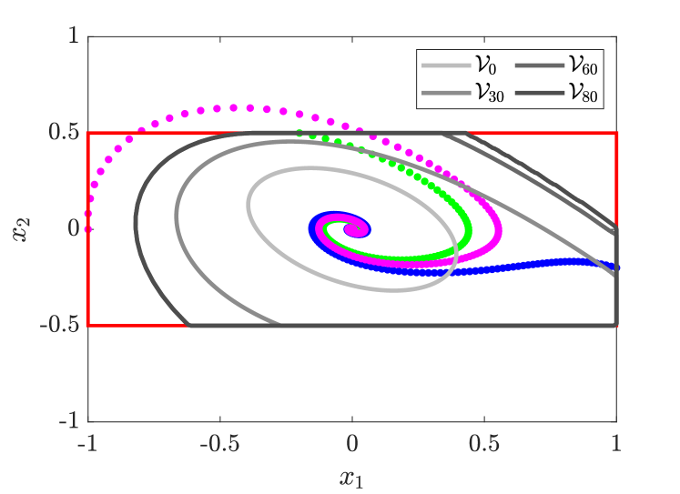
Figure 1: Estimates of the safe DOA of the two-machine system inside $\mathcal{X}$ (red), and generated trajectories starting from $\mathcal{X}$ (blue, green, and magenta).

VII-B Cart-pole system

Herein, we consider a discrete-time version of the four-dimensional controlled cart-pole system given in [23] of the form $x_{k+1}=\tilde{f}(x_{k},u_{k})$, where

$$\tilde{f}(x_{k},u_{k})=\begin{pmatrix}x_{1,k}+\Delta_{t}x_{2,k}\\ x_{2,k}+\Delta_{t}u_{k}\\ x_{3,k}+\Delta_{t}x_{4,k}\\ x_{4,k}+\Delta_{t}(\sin(x_{3,k})-\cos(x_{3,k})u_{k})\end{pmatrix},$$ (5)

$x_{1,k}$ and $x_{2,k}$ are the cart’s position and velocity, respectively, $x_{3,k}$ and $x_{4,k}$, are the pole’s angle (measured from the upright position) and angular velocity, respectively, and $u_{k}$ is the control input. The time step $\Delta_{t}$ is set to be $0.1$. It is required that the states of the system stay in the safe set $\tilde{\mathcal{X}}=\llbracket R_{\tilde{\mathcal{X}}},R_{\tilde{\mathcal{X}}}\rrbracket,$ where $R_{\tilde{\mathcal{X}}}=\begin{pmatrix}0.1&0.1&\frac{\pi}{4}&0.1\end{pmatrix}^{\intercal},$ and the control input satisfies the constraint $u_{k}\in\mathcal{U}=[-1,1]\leavevmode\nobreak\ \forall k\in\mathbb{Z}_{+}.$ Our goal herein is to safely stabilize the system around the origin by implementing a linear feedback control and estimate the DOA of the closed loop system, where the state and input constraints are fulfilled. We linearized the system at the origin, with zero control input, and computed a state-feedback control, through solving a discrete-time algebraic Riccati equation, which resulted in the gain matrix $K=\begin{pmatrix}-1.6897&-6.2464&-11.3886&-11.4026\end{pmatrix}.$ We then substituted $u_{k}=Kx_{k}$ into (5), and we obtained a closed-loop system of the form (1), with $f(x_{k})=\tilde{f}(x_{k},Kx_{k})$. For the closed loop system, the safe set $\mathcal{X}$ accounts for the state and input constraints of the open-loop system and is given as a 1-sublevel set of the function $\theta$ given by $\theta(x)=\left\|\begin{pmatrix}K\\ E\end{pmatrix}x\right\|_{\infty},\leavevmode\nobreak\ x\in\mathbb{R}^{4},$ where $E=(\mathrm{diag}(R_{\tilde{\mathcal{X}}}))^{-1}$. We then followed the procedure given in Section VI to obtain an ellipsoidal safe ROA. A hyper-rectangle that can be used in the estimation of the initial safe ROA $\mathcal{V}$ is given by $\mathcal{B}=\left\{x\in\mathbb{R}^{4}|\left\|\begin{pmatrix}K\\ E\end{pmatrix}\right\|_{\infty}\left\|x\right\|_{\infty}\leq 1\right\}$. We set $Q=\operatorname{id}_{4}$, and we obtained

$$P=\begin{pmatrix}35.6188&56.5630&60.0805&59.9877\\ 56.5630&135.0700&147.0047&146.5897\\ 60.0805&147.0047&174.9002&163.9973\\ 59.9877&146.5897&163.9973&163.6202\end{pmatrix},$$

$k=0.0312$, and an initial safe ROA $\mathcal{V}=\left\{x\in\mathbb{R}^{4}\,\middle|\,x^{\intercal}Px/k\leq 1\right\}$. We computed safe ROAs according to Theorem 5 with $60$ iterations, where their sublevel set representations are given by Theorem 6.

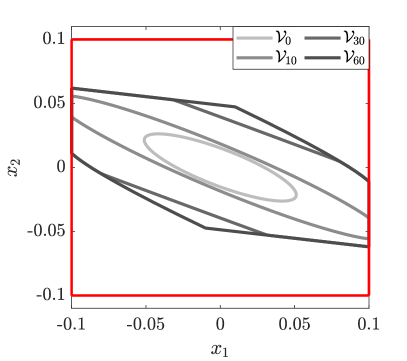
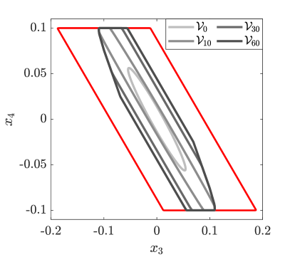
Figure 2: $x_{1}-x_{2}$ (left) and $x_{3}-x_{4}$(right) cross-sections, with $(x_{3},x_{4})=(0,0)$ and $(x_{1},x_{2})=(0,0)$, respectively, of the safe ROAs of the closed-loop cart-pole system inside $\mathcal{X}$ (red).

Cross-sections of the safe ROAs $\mathcal{V}_{0},\leavevmode\nobreak\ \mathcal{V}_{10},\leavevmode\nobreak\ \mathcal{V}_{30}$, and $\mathcal{V}_{60}$ are depicted in figure 2. Figure 2 displays the monotonicity of the resulting safe ROAs, with respect to set inclusion, and the satisfaction of the state constraints of the closed loop cart-pole system. We picked two initial conditions $x_{0}^{(1)}=[0.1\leavevmode\nobreak\ -0.02\leavevmode\nobreak\ 0\leavevmode\nobreak\ 0]^{\intercal}$ and $x_{0}^{(2)}=[-0.05\leavevmode\nobreak\ -0.05\leavevmode\nobreak\ 0\leavevmode\nobreak\ 0]^{\intercal}$ inside the set $\mathcal{X}$, and we verified, using Algorithm 1, that $x_{0}^{(1)}\in\mathcal{V}_{60}$, but $x_{0}^{(2)}\notin\mathcal{V}_{60}$. Then, we generated trajectories starting from the picked initial conditions, where the safety and convergence of the generated trajectories are verified by evaluating the function $\theta_{0}$ along the generated trajectories. Figure 3 shows how the trajectory starting from $x_{0}^{(1)}$ stays inside the safe set $\mathcal{X}$, converging to the origin , whereas the trajectory starting from $x_{0}^{(2)}$ leaves the safe set. This again displays the effectiveness of the safe ROAs obtained by our approach in certifying safe attraction.

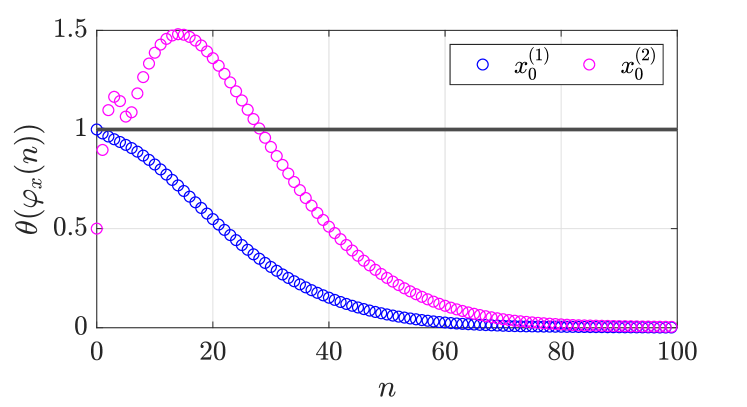
Figure 3: Profile of the function $\theta$ along the trajectories starting from $x_{0}^{(1)}$ and $x_{0}^{(2)}$.

VIII Conclusion

In this paper, we proposed an iterative approach to under-estimate safe DOAs for general discrete-time autonomous nonlinear systems using implicit representations of backward reachable sets. The sets resulting from our iterative approach are monotonic, with respect to set inclusion, and are themselves safe regions of attraction, with sublevel set representations, which are efficient for pointwise inclusion verification.

In future work, we aim to extend/adapt this framework to study robust domains of attraction and domains of null-controllability for perturbed and controlled discrete-time systems, respectively, which typically necessitate solving the computationally challenging Bellman-type equations [8].

References

- [1] J. M. Ortega, “Stability of difference equations and convergence of iterative processes,” SIAM Journal on Numerical Analysis, vol. 10, no. 2, pp. 268–282, 1973.
- [2] J. Hurt, “Some stability theorems for ordinary difference equations,” SIAM Journal on Numerical Analysis, vol. 4, no. 4, pp. 582–596, 1967.
- [3] W. Hahn, “Stability of motion,” 1967.
- [4] R. E. Kalman and J. E. Bertram, “Control System Analysis and Design Via the “Second Method” of Lyapunov: II—Discrete-Time Systems,” Journal of Basic Engineering, vol. 82, pp. 394–400, 06 1960.
- [5] S. Balint, E. Kaslik, A. M. Balint, and A. Grigis, “Methods for determination and approximation of the domain of attraction in the case of autonomous discrete dynamical systems,” Advances in Difference Equations, vol. 2006, pp. 1–15, 2006.
- [6] P. Giesl, “On the determination of the basin of attraction of discrete dynamical systems,” Journal of Difference Equations and Applications, vol. 13, no. 6, pp. 523–546, 2007.
- [7] R. O’Shea, “The extension of zubov’s method to sampled data control systems described by nonlinear autonomous difference equations,” IEEE Transactions on Automatic Control, vol. 9, no. 1, pp. 62–70, 1964.
- [8] B. Xue, N. Zhan, and Y. Li, “A characterization of robust regions of attraction for discrete-time systems based on bellman equations,” IFAC-PapersOnLine, vol. 53, no. 2, pp. 6390–6397, 2020.
- [9] A. A. Ahmadi and P. A. Parrilo, “Non-monotonic lyapunov functions for stability of discrete time nonlinear and switched systems,” in 2008 47th IEEE conference on decision and control, pp. 614–621, IEEE, 2008.
- [10] R. Bobiti and M. Lazar, “On the computation of lyapunov functions for discrete-time nonlinear systems,” in 2014 18th International Conference on System Theory, Control and Computing (ICSTCC), pp. 93–98, IEEE, 2014.
- [11] R. Bobiti and M. Lazar, “A sampling approach to finding lyapunov functions for nonlinear discrete-time systems,” in 2016 European Control Conference (ECC), pp. 561–566, IEEE, 2016.
- [12] J. Wu, A. Clark, Y. Kantaros, and Y. Vorobeychik, “Neural lyapunov control for discrete-time systems,” Advances in neural information processing systems, vol. 36, pp. 2939–2955, 2023.
- [13] H. Dai, B. Landry, L. Yang, M. Pavone, and R. Tedrake, “Lyapunov-stable neural-network control,” arXiv preprint arXiv:2109.14152, 2021.
- [14] S. Chen, M. Fazlyab, M. Morari, G. J. Pappas, and V. M. Preciado, “Learning region of attraction for nonlinear systems,” in 2021 60th IEEE Conference on Decision and Control (CDC), pp. 6477–6484, IEEE, 2021.
- [15] A. Kothyari, A. Banerjee, and P. Mhaskar, “Construction of robust ncr for input-constrained discrete nonlinear systems using backward reachability,” in 2024 American Control Conference (ACC), pp. 4954–4959, IEEE, 2024.
- [16] S. V. Raković and S. Zhang, “The implicit maximal positively invariant set,” IEEE Transactions on Automatic Control, vol. 68, no. 8, pp. 4738–4753, 2022.
- [17] K. M. Abadir and J. R. Magnus, Matrix Algebra. Econometric Exercises, Cambridge University Press, 2005.
- [18] N. Bof, R. Carli, and L. Schenato, “Lyapunov theory for discrete time systems,” arXiv preprint arXiv:1809.05289, 2018.
- [19] M. Althoff, “An introduction to cora 2015,” in Proc. of the workshop on applied verification for continuous and hybrid systems, pp. 120–151, 2015.
- [20] S. M. Rump, “Intlab—interval laboratory,” in Developments in reliable computing, pp. 77–104, Springer, 1999.
- [21] A. Vannelli and M. Vidyasagar, “Maximal lyapunov functions and domains of attraction for autonomous nonlinear systems,” Automatica, vol. 21, no. 1, pp. 69–80, 1985.
- [22] J. Willems, “Improved lyapunov function for transient power-system stability,” in Proceedings of the Institution of Electrical Engineers, vol. 115, pp. 1315–1317, IET, 1968.
- [23] M. W. Spong, “Energy based control of a class of underactuated mechanical systems,” IFAC Proceedings Volumes, vol. 29, no. 1, pp. 2828–2832, 1996.