Kilonova emission from GW230529 and mass gap neutron star-black hole mergers

Abstract

The detection of the gravitational-wave event GW230529, presumably a neutron star-black hole (NSBH) merger, by the LIGO-Virgo-KAGRA (LVK) Collaboration is an exciting discovery for multimessenger astronomy. The black hole (BH) has a high probability of falling within the “mass gap” between the peaks of the neutron star (NS) and the BH mass distributions. Because of the low primary mass, the binary is more likely to produce an electromagnetic counterpart than previously detected NSBH mergers. We investigate the possible kilonova (KN) emission from GW230529, and find that if it was an NSBH, there is a $\sim 2-41\%$ probability (depending on the assumed equation of state) that GW230925 produced a KN with magnitude peaking at $\sim 1-2$ day post merger at $g\lesssim 23.5$, $i<23$. Hence, it could have been detected by ground-based telescopes. If it was a binary neutron star (BNS) merger, we find $\sim 0-12\%$ probability that it produced a KN. Motivated by these numbers, we simulated a broader population of mgNSBH mergers that may be detected in O4, and we obtained a 9-21% chance of producing a KN, which would be detectable with $g\lesssim 25$ and $i\lesssim 24$, typically fainter than what is expected from GW230529. Based on these findings, DECam-like instruments may be able to detect up to $\sim 80\%$ of future mgNSBH KNe, thus up to $\sim 1$ multimessenger mgNSBH per year may be discoverable at the current level of sensitivity (O4).

I Introduction

In May 2023, the LIGO-Virgo-KAGRA (LVK) Collaboration started the fourth gravitational wave (GW) observing run (O4) with the Advanced LIGO [1], Advanced Virgo [2], and KAGRA [3] detector network. An exceptional GW detection occurred on May 29th 2023: GW230529 [4]. This event is of particular interest because it is likely a NSBH merger in which the mass of the primary compact object falls presumably within the $2.5-4.5~{}M_{\odot}$ range. This implies that the mass of the primary falls within the so-called lower “mass gap” between the anticipated mass range of NSs and that of BHs. Assuming an NSBH origin, it is probable that the NS has been disrupted outside of the BH’s innermost stable circular orbit (ISCO), giving rise to an electromagnetic (EM) counterpart, namely $\gamma$-ray bursts and kilonova (KN). cf. [5, 6, 7] and references therein. No GRB signatures have been found for this event [8], possibly due to the off-axis geometry of this merger, as indicated by the GW posterior constraints on the inclination angle. But in contrast to GRBs, KNe which are the ultraviolet to infrared counterparts of GWs powered by radioactive decay of the r-process nucleus [9] are expected to be more isotropic and could, therefore, even be detected for an off-axis event. Unfortunately, since GW230529 was only observed with one detector, the event’s sky location was poor, in low-latency with BAYESTAR [10] about 24,200 square degrees (at 90% credible interval - CI). Hence no online KN search has been carried out successfully for this event [11]. However, archival searches for KNe using large sky surveys may still be carried out. In addition, because GW230529-like mergers are expected to merge at a rate similar to more symmetric NSBH mergers [4], it is interesting to explore the expected KN properties and detectability for these kinds of systems.

Here, we explore 1) the possible KN signatures from GW230529 and 2) KN expectations for NSBH systems from a realistic population of mergers with the BH falling into the lower mass gap. This manuscript is organized as follows: in Sec. II, we describe the methods used to derive the KN simulations for GW230529 and for a broader mass gap NSBH (mgNSBH) population, in Sec. III, we present our results and discussion, including a comparison with works exploring similar questions [12, 13, 14]; in Sec. IV, we present our conclusions.

II Methods

II.1 Kilonova simulations for GW230529

Using the measured masses and observationally motivated arguments about the mass distribution of BHs and NSs, the LVK collaboration indicated that GW230529 likely originated from the coalescence of a BH and an NS. However, due to the non-detection of tidal effects from the GW signal, no definite conclusions were possible about the exact nature of the source. For this reason, we consider the different possibilities that exist about the nature of the binary. Within this work, we make use of the GW230529 posterior samples released in Ref. [15]. We start by considering the primary component being a BH and the secondary component a NS, first using the combined binary black hole (BBH) waveform model posterior “Combined_PHM_highSpin” [4, 16]. It is a combination of posteriors inferred from the frequency-domain model “IMRPhenomXPHM”[17, 18] and the time-domain model “SEOBNRv5PHM”[19, 20] with the spin magnitudes of the primary and secondary components restricted to $\chi_{1}$, $\chi_{2}$ < 0.99. We also use the NSBH waveform posterior “IMRPhenomNSBH” [21], which takes into account the tidal effects due to the secondary component [22] while restricting the spins to being aligned in the direction of angular momentum with values $\chi_{1}$ < 0.5 and $\chi_{2}$ < 0.05 for the primary and secondary components, respectively. This template waveform specifically models NSBH binaries for mass ratios ranging from $q=\frac{m_{1}}{m_{2}}\sim 1$ to 15, where $m_{1}$ is the mass of the primary component and $m_{2}$ is the mass of the secondary component. The Combined_PHM_highSpin results do not take into account tidal disruption. For the possibility in which also the primary component of the binary is a NS, we use the BNS waveform model “IMRPhenomPv2_NRTidalv2” [22], which takes into account the tidal effects from both primary and secondary with the spin values constrained to $\chi_{1}$ < 0.99 and $\chi_{2}$ < 0.05. We do not show results for the low-spin prior $\chi_{1},\chi_{2}$ < 0.05 posteriors as they do not produce BNS KNe given the EOSs considered, due to the samples for the primary being all above the the maximum NS mass. For all cases, including both the BNS and NSBH cases, we consider the default parameter estimation priors from the LVK analysis without taking into account population assumptions.

We compute the expected KN properties from each of these posteriors, hereafter referred to as the “BBH posterior” for posteriors assuming the Combined_PHM_highSpin waveforms, “NSBH posterior” for IMRPhenomNSBH waveforms, and “BNS posterior” for IMRPhenomPv2_NRTidalv2 waveforms, respectively. We use the Nuclear physics and MultiMessenger Astronomy framework (NMMA) [23, 24], which uses fitting formulas to connect GW source properties like compactness, mass ratio, and effective spin $\chi_{\rm eff}$ of the binary (which are fed in the form of posterior samples) to KN ejecta properties. The main outflow properties to model both BNS and NSBH KNe are the dynamical ejecta mass ($M_{\rm dyn}$) and wind ejecta mass ($M_{\rm wind}$). We use the analytical prescriptions from [25] for $M_{\rm dyn}^{\rm BNS}$, [23] for $M_{\rm disk}^{\rm BNS}$, [25] for $M_{\rm dyn}^{\rm NSBH}$ and [26] for $M^{\rm NSBH}_{\rm rem}$. For BNS mergers, $M_{\rm dyn}$ depends on the mass ratio and compactness of the merging binaries, and $M_{\rm wind}$ depends on the total mass and threshold mass. For NSBH mergers both $M_{\rm dyn}$ and the remnant mass $M_{\rm rem}$ depend on the component masses, the BH spin, NS baryonic mass and NS compactness. $M_{\rm rem}$ refers to the baryon mass around the BH 10 seconds post-merger. To obtain $M_{\rm disk}^{\rm NSBH}$ we subtract $M_{\rm dyn}^{\rm NSBH}$ from $M_{\rm rem}^{\rm NSBH}$, and then multiply by a parameter drawn from a Gaussian model to get $M_{\rm wind}$ (see Appendix A and Sec. II.B of [27] for a more detailed discussion of the equations used and ejecta parameters). Following [28, 29], and based on the findings of [30] from numerical-relativity simulations of low mass NSBH mergers, we limit the dynamical ejecta mass to be $<50\%$ of that of the remnant mass. By assuming a Gaussian prior that accounts for the fraction of $M_{\rm disk}$ ejected as wind, we derive $M_{\rm wind}$. We further require that more than $10^{-5}~{}M_{\odot}$ of ejecta mass is produced to consider a merger as producing a KN. For the fraction of these KN that could be detected, see Sec. III.3.

We carry out the fiducial analysis using the maximum posterior equation of state (EOS) from [31]. To derive further results we use the EOSs corresponding to the lower and upper 95$\%$ CI of the fiducial EOS result from [31]. Hereafter we refer to the lower and upper 95% CI as “softer” and “stiffer” EOS, respectively, so that these EOSs show how our results change for some “extreme” EOSs. We use Bu2019nsbh [32] for modeling the KN lightcurves from BBH and NSBH posteriors whereas we use Bu2019lm [23] to simulate lightcurves from the BNS posterior, which are both models based on POSSIS [33, 34], a three-dimensional time-dependent radiative transfer code. For Bu2019nsbh, the important ejecta parameters are log${}_{10}(M_{\rm dyn})$, log${}_{10}(M_{\rm wind})$ and inclination angle $\theta_{v}$ whereas for Bu2019lm, the default input parameters would be log${}_{10}(M_{\rm dyn})$, log${}_{10}(M_{\rm wind})$, $\theta_{v}$ and the half opening angle of the lanthanide-rich dynamical ejecta region $\phi$. We generate light curves in $ugrizy$ bands.

II.2 Kilonova simulations for mass gap NSBH mergers

We compare the GW230529 posterior samples with our mock population of mass gap GW events using LVK O4 sensitivities. The mass and spin distribution for this simulation is chosen from the Power Law + Dip + Break (PDB) model [35, 36, 37]. The PDB model enforces a mass “dip” between $\sim 2.2-6.0$ M_⊙, which is allowed to vary in depth. This dip between the expected NS and BH population will include events like GW230529 since it is not necessarily an empty mass gap. Because the inference for the PDB model does not significantly change with the inclusion of GW230529 [4] we use the posteriors computed based on the third GW Transient Catalog (GWTC-3; [38]). The employed pairing function ensures that component masses for a given binary tend to be similar. After drawing the samples with mass and spin distribution following the PDB model, we follow [39] and use a network SNR of 8, with the criteria that at least 1 of the detectors detect the signal above the threshold; cf. [27] for a detailed discussion of how the simulation was made.

For this work, we consider the subpopulation of simulated GW events that contains a primary in the mass gap between $\sim 2.2-6.0$ M_⊙, and we simulate KN lightcurves for the detected NSBH events. The spin ranges are set based on the component masses, with components of masses < 2.5 M_⊙ having spin magnitudes from [0,0.4] while components with masses > 2.5 M_⊙ have spin magnitudes in the range [0,1] as set in [37].

Since our distribution (which is the hyper-posterior of the PDB model fit to GWTC-3) does not depend on a binary classification, we have the freedom to define appropriate mass ranges for the astrophysical subpopulations that we consider. To differentiate between a BH and NS, we use Eq. (12) of [40], which computes the maximum mass of a uniformly rotating NS, ($M_{\rm max,{R}}$). $M_{\rm max,{R}}$ in turn depends on the maximum mass of a non-rotating NS (the Tolman-Oppenheimer-Volkoff, TOV, limit $M_{\rm TOV}$; [41, 42] ) and is therefore dependent of the EOS. For our fiducial EOS, $M_{\rm TOV,{\rm fid}}$ is 2.436 M_⊙. For the softer and stiffer EOSs, $M_{\rm TOV,{\rm l95}}$ and $M_{\rm TOV,{\rm u95}}$ are 2.069 $M_{\odot}$ and 2.641 $M_{\odot}$ respectively.

III Results and Discussion

III.1 Kilonova production from GW230529

Model	posterior	% producing KN
		softer EOS	fiducial EOS	stiffer EOS
		(%)	(%)	(%)
GW230529	BNS	1.1	7.1	11.9
	BBH	2.1	17.8	28.1
	NSBH	5.5	29.7	41.4
LVK O4	mgNSBH	8.9	17.4	21.0

Table 1: Percentage of GW230529 posterior samples or simulated O4 mgNSBH events expected to produce KN emission for each posterior model and EOS considered in this study. BNS posteriors are considered to explore the case of GW230529 being a BNS whereas the other two posteriors are considered for the case of GW230529 being an NSBH event.

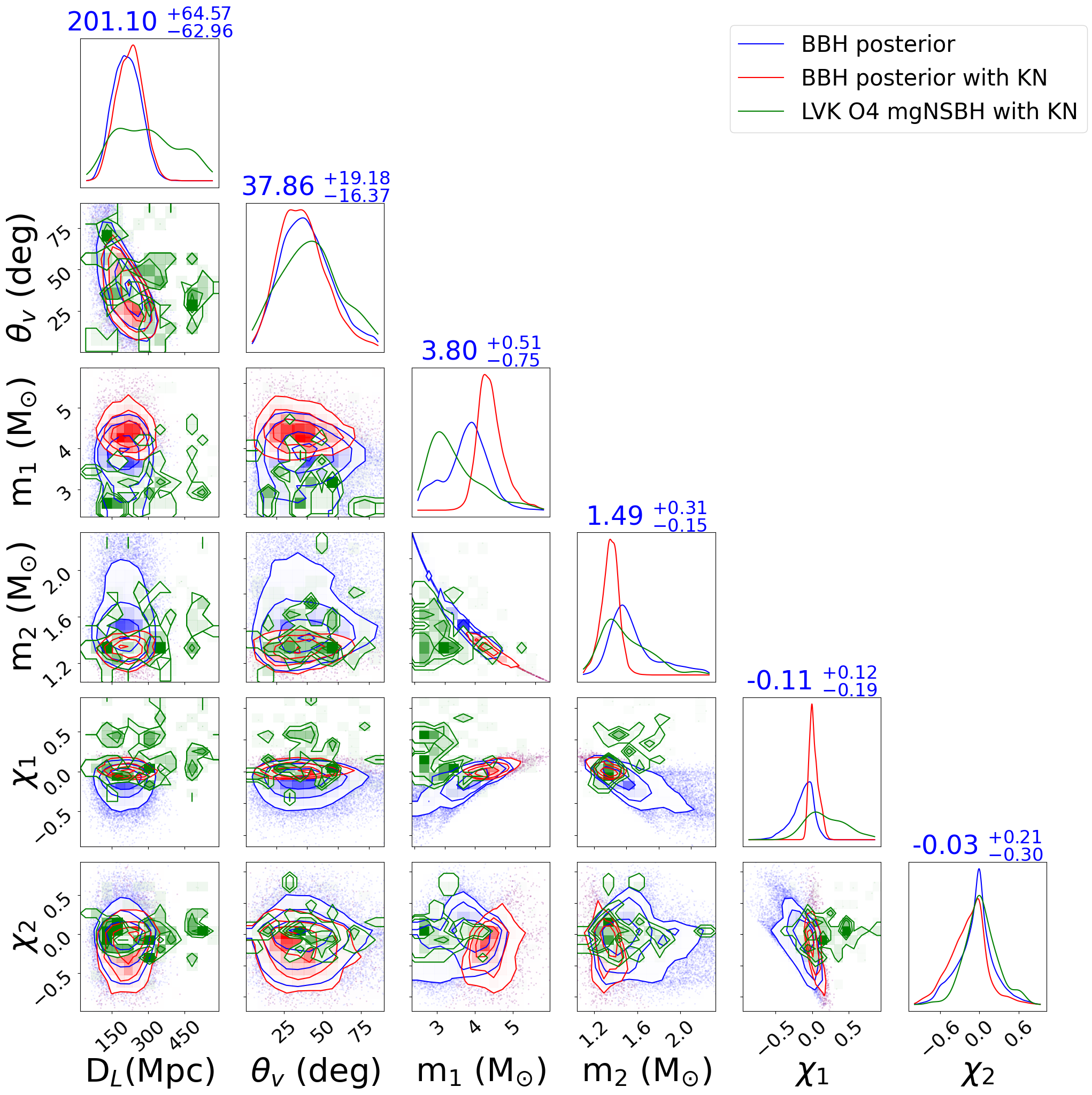
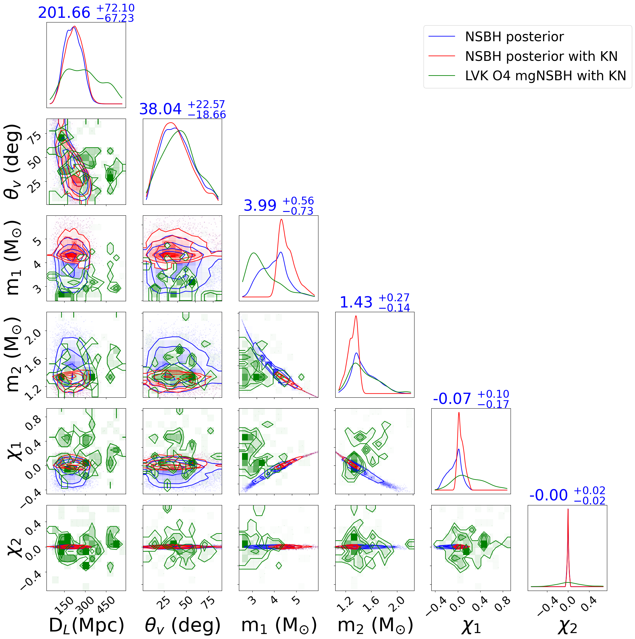
Figure 1: GW230529 binary parameters posteriors from the BBH (left) and NSBH (right) models in blue, and fraction of posterior samples that give rise to a KN (red), assuming the fiducial EOS, compared to the LVK O4 mgNSBH population producing a KN, as expected from simulations (green).

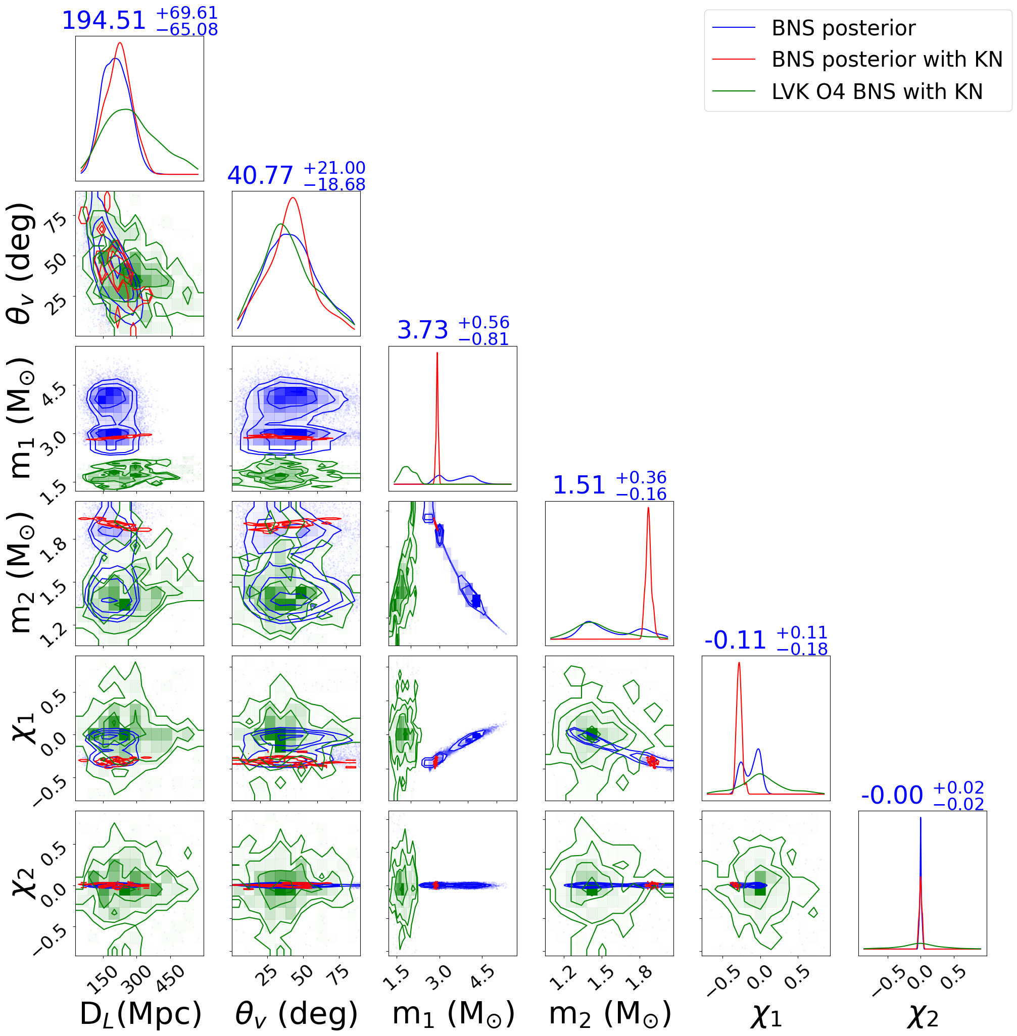
Figure 2: GW230529 binary parameters posteriors from the BNS model (blue), and fraction of posterior samples that give rise to a KN (red), assuming the softer EOS (left), and the fiducial EOS (right), compared to the LVK O4 BNS population producing a KN at luminosity distances of 100-600 Mpc, as expected from simulations (green). The values above the histograms refer to the GW230529 binary posteriors.

We start by analyzing the fraction of GW230529 posterior samples that are expected to produce a KN (i.e. the probability that this event produced a KN) under the different waveform posteriors and EOSs considered here. We also explore how the KN production prefers different parts of the binary parameter space. In Fig. 1 and Fig. 2, we show the GW230529 posterior distributions (blue) for the component masses, luminosity distance, viewing angle, and spins, assuming the BBH and NSBH posteriors, and the BNS posteriors, respectively. The red contours show the subpopulation of posterior samples that produce a KN. For the BNS case, we show both the softer and fiducial EOSs for comparison, as the differences are more noticeable in this case. The percentages of posteriors producing a KN for each model and each EOS considered are summarized in Table 1.

First, we note that only a subdominant fraction of the samples produces a KN in all cases. We attribute this to the degeneracy between $m_{1}$ and $m_{2}$, as a redshifted chirp mass is measured from the GW data, and individual component masses are not as well constrained. As a result, the parameter space allowed by the posterior that favors a lower $m_{2}$, which is typically expected to produce more ejecta mass than a more massive secondary all other parameters being fixed, is bound to larger values of $m_{1}$, which on the other hand is not favorable for KN production. Moreover, the effective spin is likely negative or close to $0$, with a probability of $\sim 83\%$ of the primary spin to be anti-aligned [4], which further reduces the probability of producing a KN in an NSBH system as it increases the BH ISCO radius compared to a BH of the same mass spinning in the same direction as the binary angular momentum. As a result, only a specific subset of posterior samples can produce a KN. This subset will depend on the posterior support at low secondary mass, as well as on the spins of the NS along with the EOS. These factors can increase the maximum NS mass, and the spin of the BH, which affects the ISCO radius; cf. e.g. [43, 5] and references therein.

As we go from softer to stiffer EOSs the distribution of $m_{2}$ where a KN is produced shifts towards higher masses as these become allowed (see Fig. 2 for the BNS case). This results in the distribution for $m_{1}$ shifting towards lower masses due to the degeneracy between $m_{1}$ and $m_{2}$ from the GW parameter estimation. This is true for all 3 cases - BNS, NSBH, and BBH models.

For what concerns GW230529 as an NSBH, considering the case of NSBH (BBH) posteriors, $\sim$ 6-41 % (2-28 %) of cases produce a KN, with the stiffer EOS giving the largest number. One major difference between the BBH and NSBH posteriors, which is expected to affect our results, is the prior on the spin for both the primary and secondary, which affects the maximum NS mass allowed as well as the BH ISCO radius. The NSBH posteriors achieve larger fractions for a successful KN production, mainly due to a combination of the following: the BH spin in the BBH model has a tail at $\chi_{1}<-0.4$, which is not allowed by the NSBH model prior, and disfavors KN production as it increases the ISCO radius compared to greater spin values; and the primary mass posterior for NSBH shows more support at lower secondary masses ($m_{2}\lesssim 1.5$) than for the BBH case.

For the BNS posterior, the spin of the primary component $\chi_{1}$ allows for larger spin magnitudes than for the secondary, which in turn allows for more massive NSs to exist and hence produce a BNS KN, but only in the case of anti-aligned spin as the aligned case is not favored by the GW data. This implies that for the BNS case, the EOS that allows the largest portion of parameter space in the fast, anti-aligned primary spin region, given the degeneracy between $m_{2}$, $m_{1}$, and $\chi_{1}$, is most likely to produce an EM signal. As one may have expected, the softer EOS is less likely to produce a KN ($\sim 1\%$), and the probability grows as we move to the fiducial ($\sim 7\%$) and stiff ($\sim 12\%$) EOS.

For the BNS model, assuming the softer EOS, only a specific configuration of the component masses and spins allows for a KN. The configuration is the one that gives the highest possible mass given the allowed values of spin for the primary component, while still allowing it to be a NS, as shown in the left panel of Fig. 2. The configuration does not allow more negative spin values or lower $m_{1}$ since it would require $m_{2}$ to be more massive. However, that is not allowed since the posteriors of $m_{2}$ are limited by the spin prior to $\chi_{2}<0.05$, so the highest possible mass $m_{2}$ can take is very close to M_TOV,l95. For the fiducial EOS, since the secondary component can reach higher mass, the primary component is allowed to reach more negative spins.

Next, we discuss the predicted ejecta mass from the simulated KNe. In the GW230529 NSBH KN case, $M_{\rm wind}$ is the lowest for softer EOS and the highest for the stiffer EOS, while the dynamical ejecta has a median ranging from $10^{-3.05}-10^{-2.32}~{}M_{\odot}$ for the NSBH posterior and from $10^{-3.10}-10^{-2.56}~{}M_{\odot}$ for the BBH posterior as shown in th top panels of Fig. 3. This agrees with estimated ejecta masses between $4\times 10^{-3}$ and $5\times 10^{-2}$ from numerical simulations of low-mass NSBH binaries [30].

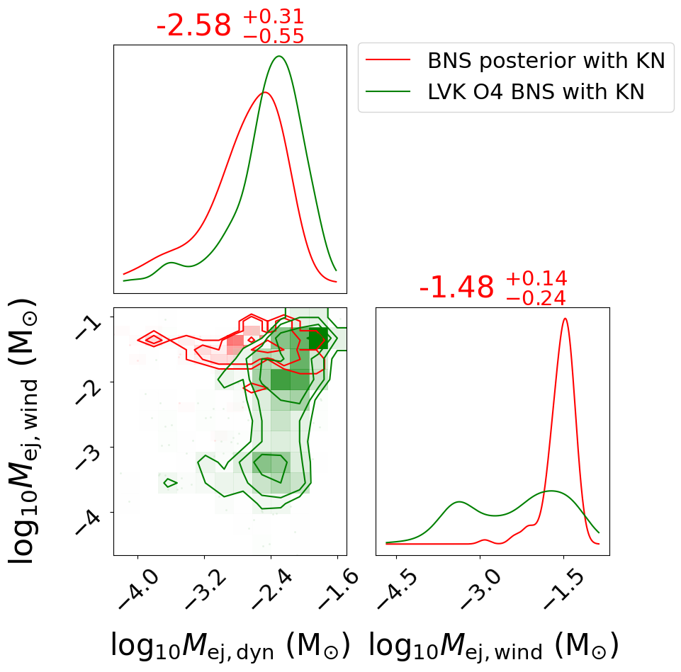
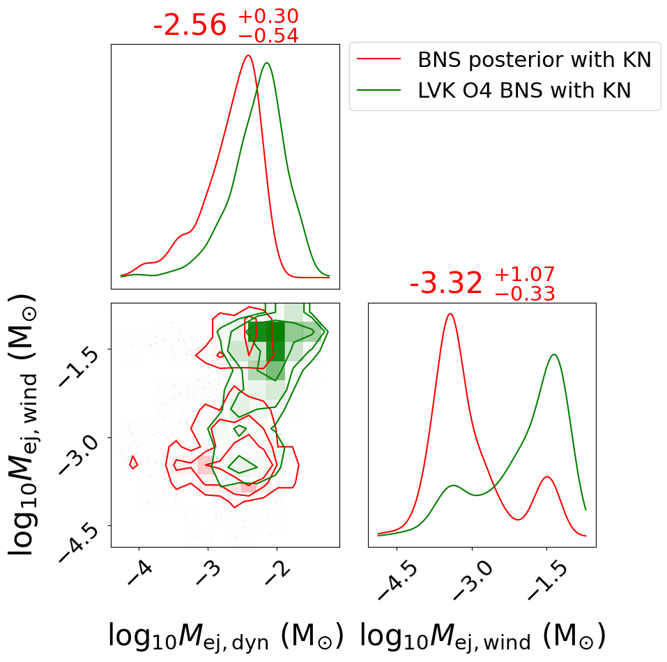
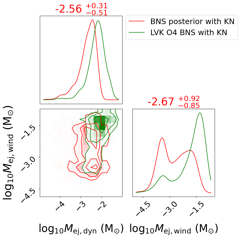
Figure 3: GW230529 cornerplots of dynamical and wind ejecta mass, in red, for the case of NSBH KN production assuming the GW230529 BBH posterior (top panels), and BNS KN from the BNS posterior (bottom panels), a softer (left panels), fiducial (middle panels), and stiffer (right panels) EOS. The green contours show the expected population from mgNSBH (top) BNS mergers (bottom) expected to be detected at O4 sensitivity.

In the case of GW230529 being a BNS, assuming the softer EOS, we expect more wind ejecta than dynamical ejecta, with large values of the order of $10^{-2}~{}M_{\odot}$. This is not the case with the fiducial and stiffer EOS, for which the BNS is expected to produce typically more dynamical than wind ejecta (with the latter peaking close to $\sim 10^{-2.6}~{}M_{\odot}$ for all EOSs). This is not surprising as the disk mass fitting formula, from which the wind ejecta mass is then derived, for BNS systems depends entirely on total mass and threshold mass, which is sensitive to the EOS. The larger $M_{\rm tot}$ values allowed by the fiducial and stiffer EOSs compared to the soft EOS case do not result in large disks. On the other hand the dynamical ejecta mass is highly sensitive to the mass ratio, which does not span a large dynamical range for the BNS samples producing a KN, hence providing similar amounts of dynamical ejecta in all cases (see e.g. [23, 25] for a detailed discussion on the equations governing the ejecta masses). The dynamical ejecta mass distribution is also similar to that of the NSBH case. The dynamical ejecta mass for GW230529 as a BNS is, as expected given the large masses, typically lower than for our BNS population expected from O4 at a similar distance, and it is shifted by 0.3-0.5 dex towards lower values (see Fig. 3).

A caveat of this analysis is that the surrogate models used in NMMA are built on POSSIS grids with a minimum $M_{\rm dyn}$ of 0.001 (0.01) $M_{\odot}$ and $M_{\rm wind}$ of 0.01 (0.01) $M_{\odot}$ for Bu2019lm (Bu2019nsbh). Therefore for ejecta masses below these values, a fraction of the KNe we consider follow an extrapolation.

At last, we note that, as expected, the normalized luminosity distance and viewing angle distributions of the samples producing a KN are similar to these in the input posterior, since these extrinsic parameters do not have an impact on the production of a KN, but we show them for comparison with the broader mgNSBH population.

III.2 Kilonova production from a mass gap NSBH merger population

In this section, we show predictions for KN production of LVK O4 mgNSBH mergers and compare those to the potential KN emission from GW230529. We also include a comparison for simulated O4 BNS KNe at distances similar to GW230529. Fig. 1 and 2 show the respective O4 populations with green contours and distributions.

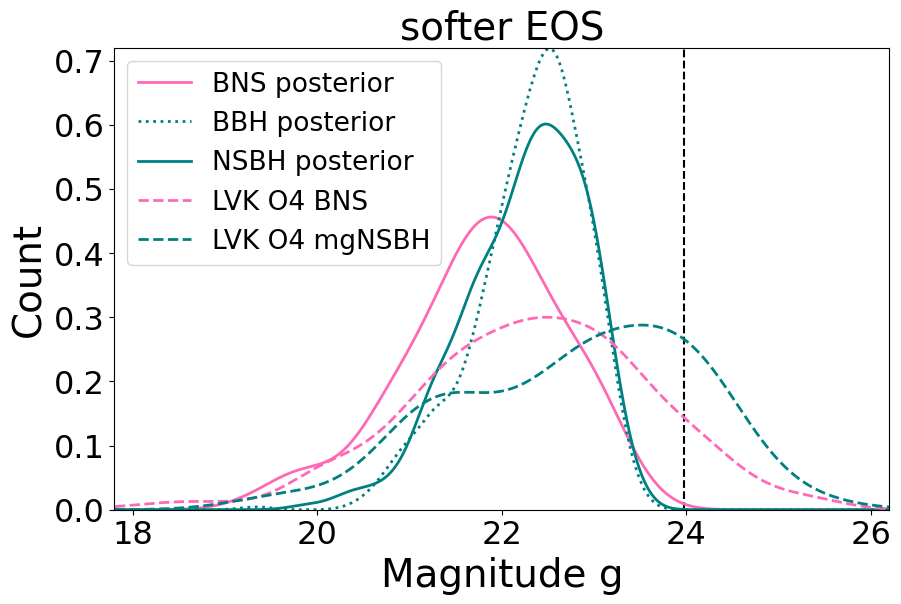
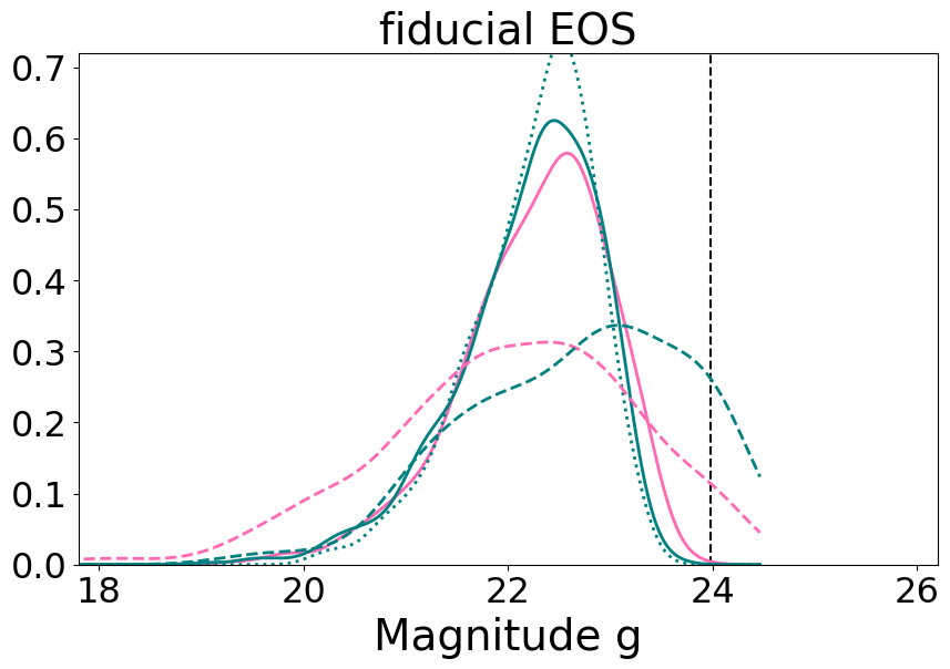
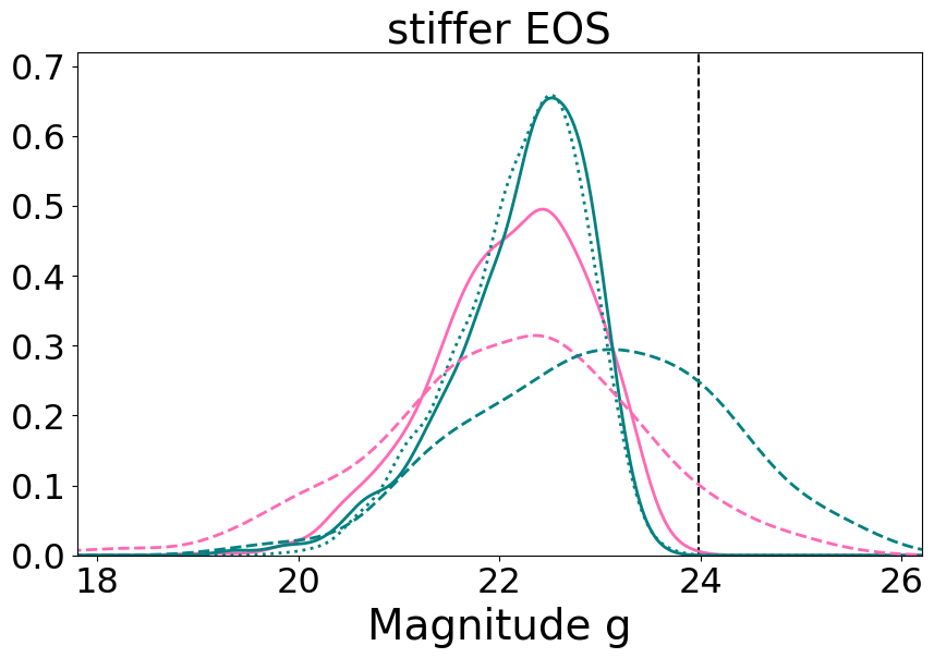
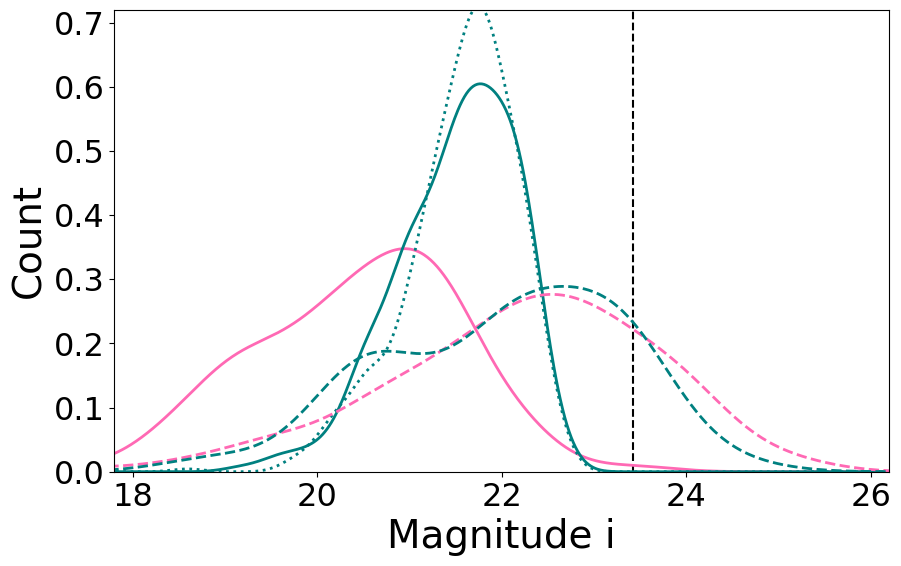
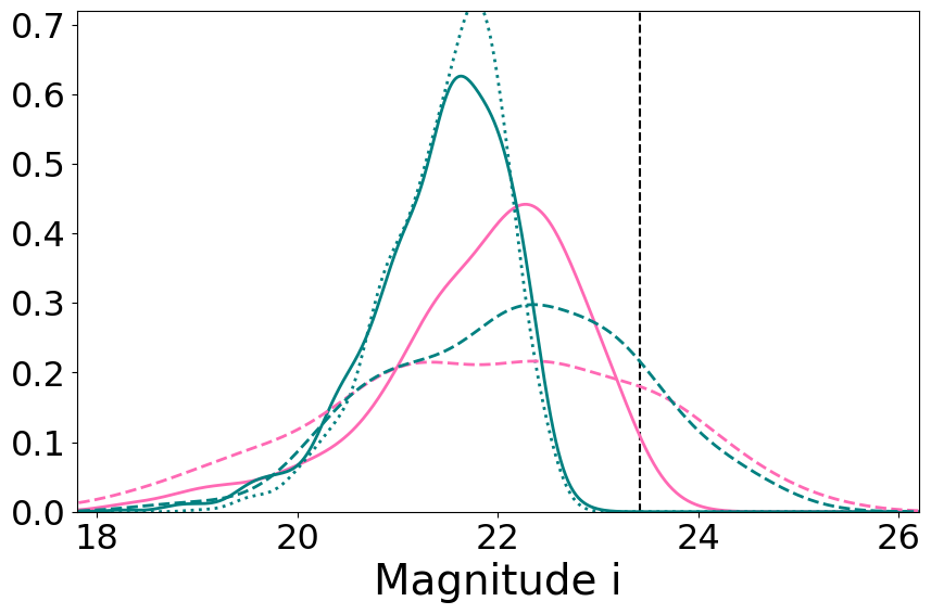
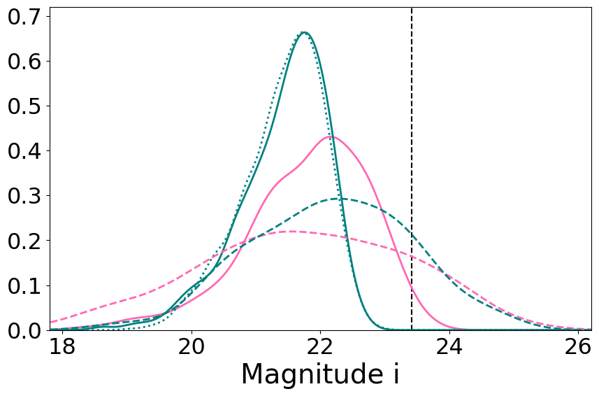
Figure 4: Simulated KN $g$ (top panels) and $i$ (bottom panels) magnitudes produced at 1 day post merger for different GW230529 posterior models (solid lines), and for the LVK O4 simulations of mgNSBH mergers and BNS mergers at 150-250 Mpc (dashed lines). The left-hand side panels assumes a soft EOS, the middle panels assume our fiducial EOS, and the right-hand side panels assume a stiff EOS. The black dotted line represents a reference DECam $5\sigma$ depth limit for an exposure time of 90s in the respective filters.

We start by analyzing the KN emission from our simulated LVK O4 mass gap events. Table 1 shows the percentage of these NSBH merger events that produce a KN based on the EOS considered. Here, we see a trend similar to that of the GW230529 BBH posterior where the softer EOS results in the least KN production and the stiffer EOSs result in higher KN production. By comparing the posteriors in Fig. 1, we note that $\chi_{1}$ shows a preference for an anti-aligned spin for the GW230529 BBH and NSBH KN populations, as opposed to a preference for an aligned spin in the LVK O4 KN distribution (85% of samples for the softer EOS to 76% for the stiffer EOS). This is mostly because the majority of the GW230529 posterior samples (82$\%$ for BBH and 72$\%$ for NSBH) do not allow for positive spin of the primary. The input distribution for LVK O4 has spins that are uniform in magnitude and isotropic in orientation, which for events producing a KN is slightly shifted towards aligned $\chi_{1}$. For more asymmetric NSBHs, spin should have an even more significant effect on tidal disruption compared to what is expected for GW230529 [14]. However, such configurations are rare in our simulations due to the assumed pairing function (which is found from a fit of GWTC-3) favoring more equal mass even for binaries containing a low mass secondary $m_{2}<3~{}M_{\odot}$ (the rate of an NSBH with a BH 5 times the mass of the NS as in [14] is suppressed by a factor of $\sim 4$ compared to more equal mass binaries), although less strongly than what is found for BBHs. Regarding $\chi_{2}$, the LVK O4 distribution allows for a wide range of spins with similar preference for aligned and anti-aligned spins, while the GW230529 BBH KN distribution shows a preference for events with anti-aligned NS spin, which is a result of the degeneracy between $\chi_{1}$, $m_{1}$, and $\chi_{2}$, and the fact that lower $m_{1}$ is preferred for KN production. We note similar trends for mass and spin distributions for the other two EOSs.

As noted above, the degeneracy between $m_{1}$ and $m_{2}$ results in a strong preference for lower $m_{2}$ and higher $m_{1}$ in the GW230529 KN production. LVK O4 mgNSBH KNe occupy a different region of parameter space. Due to more equal mass binaries being preferred (and allowed) as opposed to asymmetric masses, and the fact that merger rates for objects in the dip (starting around $\sim 3~{}M_{\odot}$) are also suppressed as higher masses are reached, mgNSBHs producing KNe tend to more likely have a BH of 3-4$M_{\odot}$, rather than the $\sim 4~{}M_{\odot}$ BH required for GW230529 to produce a KN. Moreover, because of the pairing and the wide NS spin prior, the mgNSBH O4 KN population has a secondary mass distribution that extends to 2 $M_{\odot}$ also with the fiducial EOS. Also [44], starting from an isolated binary population, find that the majority of NSBH KNe are produced by mgNSBHs with a massive NS.

The viewing angle distribution of both the mass gap events and GW230529 follow a Schutz distribution [45] due to the GW selection effects and peak around $\sim 35$ deg, i.e., it is unconstrained for GW230529 and recovers the prior. The luminosity distance of possible O4 mgNSBH detections peaks at $\sim 310$ Mpc and falls off between 400 and 600 Mpc.

For what concerns the ejecta mass, the dynamical ejecta mass distribution from the mgNSBH KN O4 simulations are found to be similar to those of GW230529 with a median ranging from 10${}^{-2.6}~{}M_{\odot}$ for the softer EOS to 10${}^{-2.1}~{}M_{\odot}$ for the stiffer EOS. Wind ejecta are also significant with a median around 10${}^{-2.6}~{}M_{\odot}$ for softer EOS to 10${}^{-2.1}~{}M_{\odot}$ for stiffer EOS.

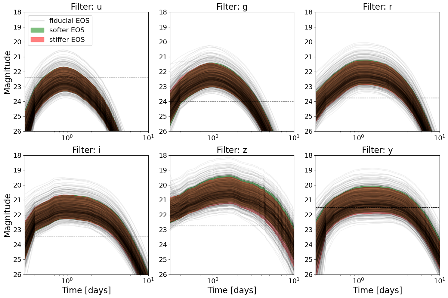
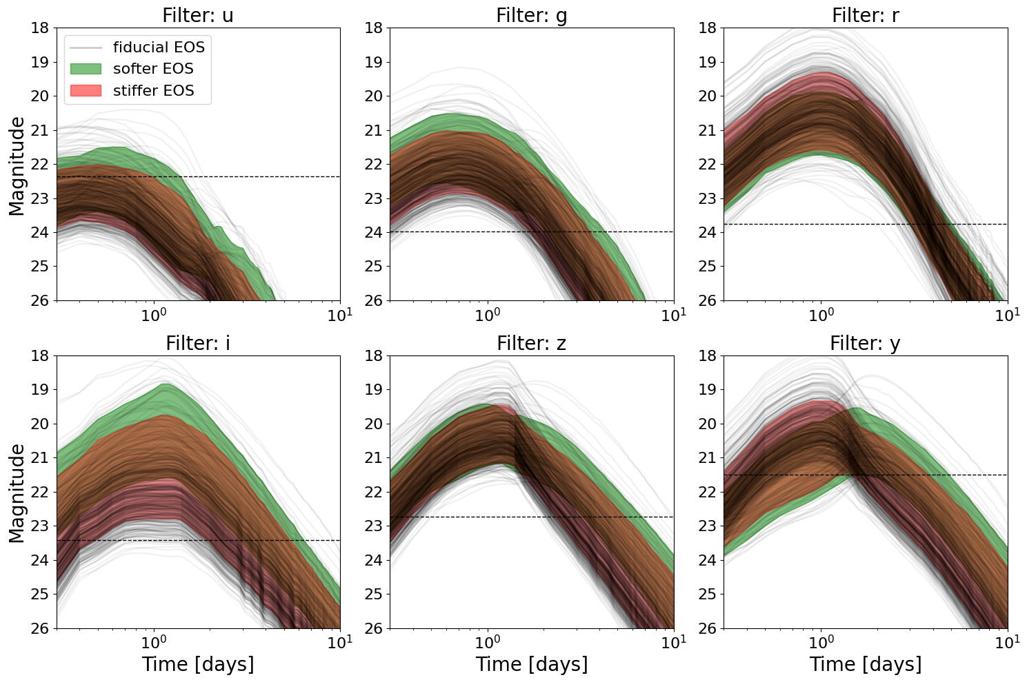
Figure 5: Simulated KN light curves from 0.3 days to 10 days after the merger, in $ugrizy$ expected from GW230529 assuming the BBH (top six panels) and BNS posteriors (bottom six panels). The black lines show the light curves corresponding to our fiducial EOS for 500 randomly sampled KNe for visualization purposes. For comparison, light curves from the softer and stiffer EOS are shown as filled regions in green and red, respectively, representing the range of magnitudes between the 10th and 90th percentile of the simulated population. The black dotted line represents a reference DECam $5\sigma$ depth limit for an exposure time of 90s in the respective filters.

III.3 Kilonova detection

We generate light curves in $ugrizy$ bands up to 10 days from the merger for all 3 EOSs under consideration. First, we discuss the KN magnitudes produced at 1 day post merger for the 3 GW230529 posterior models, LVK O4 mgNSBH simulations and LVK O4 BNS simulations as shown in Fig. 4. Note that in this plot, we limit the luminosity distance range for the events from our LVK O4 simulations to 150-250 Mpc, for a better estimate of events that share similar parameter space as that of GW230529, which was reported to be at a median distance of $\sim 200$ Mpc [4].

In both $g$ and $i$ bands, except for the softer EOS, the LVK O4 BNS KNe show a tail at higher luminosity compared to the GW230529 BNS KN, since the GW230529 BNS posterior is massive compared to the general BNS population and would, therefore, likely produce less ejecta mass for a given EOS. The LVK O4 BNS KNe also show a tail at larger magnitudes because the O4 population distance distribution is flatter and extends to larger distances compared to that of GW230529. The bright magnitudes found for the GW230529 BNS case are due to the large wind ejecta masses discussed in the previous subsections for the small fraction ($\sim 1\%$) of posterior samples that allow KN production. The LVK O4 BNS population also produces typically brighter KNe compared to the mgNSBH cases.

Model	posterior	KN Percentage detectable by DECam
		$u$	$g$	$r$	$i$	$z$	$y$
GW230529	BNS	15-16	72-100	72-100	72-99	72-100	64-98
	BBH	22-33	71-99	71-99	71-99	71-99	48-75
	NSBH	22-34	78-99	78-99	78-99	78-99	45-65
LVK O4	mgNSBH	21-22	64-73	63-72	75-84	77-86	34-38

Table 2: Probability that the GW230529 KN could have been detected with DECam at 5$\sigma$ depth limit for a 90s exposure time, assuming different posterior models. We also show probabilities for a generic mass gap population from our LVK O4 simulation.

The GW230529 BBH and NSBH posteriors produce very similar KN lightcurves. The median peak magnitudes assuming the NSBH posteriors for softer, fiducial, and stiffer EOSs are $\sim$ 22.35, 22.31, 22.36 for $g$-band and $\sim$ 21.6, 21.52, 21.55 for $i$-band respectively. $i$-band appears to be brighter than $g$-band for models with NSBH KN as well as for the BNS posterior.

It is interesting to note that also the broader population of mgNSBH mergers detectable in O4, assuming they follow the population models assumed here, is likely to produce KNe with $g\lesssim 25$ and $i\lesssim 24$, and would therefore be observable by a range of telescopes.

We show full light curves for a KN from GW230529 in Fig. 5. We only consider light curves starting at 0.3 days post merger to avoid extrapolation issues from the surrogate models. The NSBH KN light curves are typically red, appear to be brightest in the $z$-band, and peaking between day 1 and 2. Overall, we expect the KN to be broadly detectable by ground-based instruments in all bands except for $u$. We consider for reference the detection limit of the Dark Energy Camera (DECam; [46]). DECam is a wide-field, high-performance CCD camera mounted on the 4m Blanco Telescope in Chile, and it is a major telescope used for GW follow-up in O4 by GW-MMADS (Gravitational Wave Multi-Messenger Astronomy DECam Survey; [47]). In Table 2, we report the expected probability that, if GW230529 produced a KN in an observable region of the sky, it could have been detected by DECam with 90s exposures in gray time, assuming our fiducial EOS. We provide a range of detection fractions, where the low limit is given by the fraction of detected samples with at least one ejecta component more massive than $0.001~{}M_{\odot}$, while the high limit takes also lower ejcta mass systems into account. This allows us to estimate the fraction of detectable systems excluding the more extreme extrapolations by the surrogate models, as described in Section III.1. For both BNS and NSBH KN, the lowest percentage is observed in $u$-band. For the BNS posterior, it is followed by the remaining bands with around 60-100$\%$ of the samples being detectable by DECam. If GW230529 is an NSBH and it produced a KN, we have about $70-99\%$ probability we could have detected it in $griz$ bands. We note that on the other hand, a search going to mag $\sim 20.5$ such as that presented in [11] from Zwicky Transient Facility data, was unlikely to detect the predicted KN signal.

In the LVK O4 mgNSBH simulation, we note that $u$ and $y$ bands show the lowest and highest KN detection. Up to $77-86\%$ of mgNSBH KNe in O4 should be detectable by DECam-like instruments, with the highest efficiency in $z$ band. Note that efficiencies are lower for O4 mgNSBH KNe than for GW230529 and the O4 KNe shown in Fig. 4 as here we are considering any distance present in our GW simulations, going beyond that of GW230529.

The difference between lightcurves from different EOSs is minimal in the case of the NSBH KNe, with median peak $g$ magnitudes up to 0.2 mag brighter for the stiffer EOS compared to the softer one, since the former typically allows for easier NS disruption. The luminosities evolve slowest in $z$-band and fastest in $u$-band, and peak around day 2 for $rzy$ bands and around day 1 for $u$ and $g$ bands, with $i$-band luminosities peaking around 1.5 days after the merger. For the NSBH KNe, we only show light curves assuming the BBH model and not the NSBH one, as they are very similar.

The KNe expected from the GW230529 BNS posterior exhibit more diversity than those produced by the BBH and NSBH posterior. The BNS light curves peak around 8h from the merger and have a faster evolution in the bluer bands. Overall, we still find a significant probability that we could have detected the KN from GW230529, assuming it arose from a BNS merger and it did indeed eject enough mass. Moreover, it is clear that orders of magnitude differences are present in the light curves between the BNS and NSBH cases so observations of a KN in coincidence with an event like GW230529 will allow us to discern between different kinds of binaries when the GW data are not sufficient [28]. Typically the KNe from NSBH mergers may be brighter than those from high mass BNSs, e.g., [28, 48], owing to the fact that such BNSs would produce low mass dynamical ejecta and disks.

III.4 Comparison with other works

The GW230529 discovery article [4] includes a computation of the expected remnant mass outside of the final black hole, which we also compute here to estimate the NSBH ejecta masses, and can be used as a probe of KN production. After marginalizing over a range of EOSs, for the BBH posteriors, they find a 10% probability that some of the NS material is disrupted outside of the BH, which is consistent with the range of values we find of 2-28% for KN production assuming the same posteriors. Ref. [4] also measures the remnant mass for the low-spin prior BBH posteriors, which we do not take into account here, finding a 4% probability of NS disruption.

In Ref. [49], the authors use the available prior models to evaluate the possible mechanisms leading to the formation of GW230529. They also ascertain which component of the merger formed first: NS or BH, and use the posterior samples to characterize the remnant BH. Whereas in our work our primary focus is to explore the nature of KN emission and to constrain the parameter space that leads to such EM emissions. They compute ejecta masses for an expected population of mgNSBHs from isolated binaries using 4 EOSs: APR4 [21], SLy [50], DD2 [51] and H4 ([52]), whereas we compute KN lightcurves using the maximum posterior EOS from [31] and its upper and lower 95% CI to estimate the effect of stiffer and softer EOS on KN detectability for both GW230529 and a population of mgNSBH binaries. They expect a peak KN luminosity for the mgNSBH population ranging from 26.63 - 24.04 from $u$ - $y$ bands, which is typically dimmer than what we predict based on the EOSs under consideration, which we attribute to the different population assumed and KN models. However we note that our mgNSBH O4 population magnitude predictions are very broad and overlap with their findings (see Fig. 5).

In [12], the authors use the combined posterior Combined$\_$PHM$\_$lowSecondarySpin to study GW230529 and compare it to GW events GW200105, GW200115 to explore the formation channel and possible EM counterparts of GW230529, whereas we use Combined$\_$PHM$\_$lowSecondarySpin along with 2 other posteriors corresponding to NSBH and BNS waveforms to take into account different KN emission from this merger. They find overall a high probability of producing a KN, up to 60%, and KN dimmer than what we find by up to $\sim 1$ mag (although the difference is not as extreme as that with [49]), which we attribute to the different assumptions used: EOS, fitting formulae for the ejecta mass, and KN modeling.

For the population of expected mgNSBH simulations, they use COMPAS, a rapid binary population synthesis code from [53], in our article, we use a data-driven approach and assume a compact object population that follows the PDB model from [36] based on LVK detections. Our results on KN detectability agree since we both predict the peak apparent magnitude of GW230529 KN to be $\sim$ 23-24 mag in g and r bands.

IV Conclusion

In this article, we explore the possible KN emission signatures from the GW event GW230529. To take into account different possibilities regarding the nature of the components, we perform the analysis using BBH, NSBH, and BNS waveform posterior of this event. For both the BBH and NSBH posteriors, we assume that NSBH KN can be produced. We find that if GW230529 is indeed an NSBH, there is a 2-41$\%$ probability that it produced a KN, depending on the EOS under consideration; whereas, if GW230529 is a BNS, there is 0-12$\%$ chance of a KN emission. We include 0% probability of producing a KN even though our results show a minimum of 1% to take into account the case of the low-spin prior BNS posteriors which cannot produce a KN due the primary samples being above the maximum NS mass given the EOSs considered.

Firstly, we explore the parameter space of the posteriors that resulted in KN emission. KN production favors lower $m_{2}$, but the degeneracy between $m_{1}$ and $m_{2}$ results in higher $m_{1}$ to be associated with a low-mass NS, which disfavours KN production. As a result, across all posterior models, KN production is supported by lower $m_{2}$ and higher $m_{1}$. The NSBH posteriors support slightly larger KN production than the BBH posterior, likely due to: i) the lower BH spin allowed in the BBH posterior results in a higher ISCO radius which disfavors KN production, and ii) the NSBH posterior showing more support for $m_{2}\leq 1.5~{}M_{\odot}$ than the BBH posteriors, and lower $m_{2}$ implies higher KN production.

We utilize the Power Law + Dip + Break model to simulate mgNSBH mergers expected during the fourth LVK observing run O4 and to compare the results with GW230529, for a better understanding of its position in the parameter space of our simulation and of prospects for future detection of EM counterparts to mgNSBHs. The $\chi_{1}$ spin distribution shows a slight preference towards positively aligned spin. Without the chirp mass posterior degeneracy, KN production is supported by lower $m_{1}$ values ($\sim 3-4~{}M_{\odot}$) in the LVK O4 mgNSBH population compared to the GW230529 NSBH case ($\sim 4~{}M_{\odot}$).

Out of the 7$\%$ of BNS posterior samples that result in a KN with our fiducial EOS, $\sim 70-100\%$ are detectable by DECam in $griz$ with a 90s exposure time, depending on the filter. The magnitude would peak around 1 day post merger at $g,i<23$.

If GW230529 produced an NSBH KN and it was in an observable region of the sky, there is a $\sim 70-99\%$ of the samples could have been detected by DECam–like instrument in $griz$. The detection magnitude would peak at $g<24,i<23$ and around 1 day post-merger for $ug$, 1.5 days post merger for $ri$ and around 2 days post-merger for $zy$ bands.

KN emission from LVK O4 mgNSBH mergers is typically dimmer in optical apparent magnitude than the expected emission from GW230529, and can extend out to 600 Mpc. With ground-based telescopes like DECam, it would be wise to trigger follow-up observations at the redder wavelengths, with $i$ or $z$-band, which have the highest probability of detecting a KN at 75-86%, followed by $gr$ bands at $\sim$ 63-73% out of the 17% of KNe produced assuming the fiducial EOS. The expected detection rate for mgNSBH events based on the distribution [36] and detection criteria we use to simulate LVK O4 events is $\sim 5$/year, therefore $\lesssim 1$ event per year may produce a KN with significant probability of detection. Overall, we find that mgNSBH mergers may represent a promising class of multimessenger sources in the near future.

Appendix A Ejecta mass fitting formulae

The equations used to calculate the ejecta masses are summarized below. For BNS mergers, we follow the relation from [25] to model the dynamical ejecta mass $M_{\rm dyn}$:

$$\frac{M_{\rm dyn}^{\rm BNS}}{10^{-3}}=\left(\frac{a}{C_{1}}+b\left(\frac{M_{2}}{M_{1}}\right)^{n}+cC_{1}\right)M_{1}+(1\leftrightarrow 2).$$ (1)

Here, the compactness $C_{1}$ is $GM_{1}/R_{1}c^{2}$, where $M_{1}$ and $R_{1}$ are the mass and radius of the primary (similarly for the secondary), and the best-fit parameters from the numerical simulations are $a=-9.3335$, $b=114.17$, $c=-337.56$ and $n=1.5465$ [25].

The disk mass for BNS mergers follows the relation from [23]:

$$\log_{\rm 10}\left(M_{\rm disk}^{\rm BNS}\right)=\max\left(-3,a\left(1+b\tanh\left[\frac{c-{M_{\rm tot}}/{M_{\rm th}}}{d}\right]\right)\right),$$ (2)

where $M_{\rm th}=k_{\rm th}M_{\rm TOV}$ is the threshold mass [54], $k_{\rm th}$ is a function of $M_{\rm TOV}$ and EOS [55], $a$ and $b$ are functions of the mass ratio $q$. These parameters are given by:

$$\begin{split}&a=a_{0}+\delta_{a}x_{i}\\ &b=b_{0}+\delta_{b}x_{i}\\ &x_{i}=0.5\tanh(\beta(q-q_{t}))\\ \end{split}$$ (3)

where $a_{0}=-1.581$, $b_{0}=-0.538$, $c=0.953$, $d=0.0417$, $\delta_{a}=-2.439$, $\delta_{b}=-0.406$, $\beta=3.910$, and $q_{t}=0.900$.

For NSBH mergers, the dynamical ejecta mass is given by the equation from [25]:

$$\frac{M_{\rm dyn}^{\rm NSBH}}{M_{\rm NS}^{b}}=a_{1}Q^{n_{1}}\frac{1-2C_{\rm NS}}{C_{\rm NS}}-a_{2}Q^{n_{2}}\frac{R_{\rm ISCO}}{M_{\rm BH}}+a_{4}$$ (4)

where the best fitting parameters are $a_{1}=0.007116$, $a_{2}=0.001436$, $a_{4}=-0.02762$, $n_{1}=0.8636$ and $n_{2}=1.6840$. Here $Q={M_{\rm BH}}/{M_{\rm NS}}$ where the mass ratio is defined as $q=1/Q$ and $R_{\rm ISCO}$ is the radius of the innermost stable circular orbit (ISCO) of the black hole with mass $M_{\rm BH}$ and spin $\chi_{\rm 1z}$ in the direction of the orbital angular momentum. The NS baryonic mass is given by $M_{\rm NS}^{b}$ = $M_{\rm NS}\left(1+\frac{0.6C_{\rm NS}}{1-0.5C_{\rm NS}}\right)$ [56], where $C_{\rm NS}$ is the compactness of the NS.

For NSBH mergers, the remnant mass, which is used to refer to the baryon mass outside the BH $\sim 10$ ms post-merger, is calculated using the fitting formula by [26]:

$$\hat{M}^{\rm NSBH}_{\rm rem}=\left[{\rm max}\left(a\frac{1-2C_{\rm NS}}{\eta^{1/3}}-b~{}R_{\rm ISCO}\frac{C_{\rm NS}}{\eta}+c,0\right)\right]^{1+d}.$$ (5)

Here $\eta$ = $Q/(1+Q^{2})$ is the symmetric mass ratio, $\hat{M}$ = $M^{\rm NSBH}_{\rm rem}/M^{\rm b}_{\rm NS}$ and $a=0.40642158$, $b=0.13885773$, $c=0.25512517$, $d=0.761250847$. The disk mass $M^{\rm NSBH}_{\rm disk}$ is calculated by subtracting $M^{\rm NSBH}_{\rm dyn}$ from $\hat{M}^{\rm NSBH}_{\rm rem}$ with remnant mass zero corresponding to no tidal disruption.

References

- Aasi et al. [2015] J. Aasi et al. (LIGO Scientific), Class. Quant. Grav. 32, 074001 (2015), arXiv:1411.4547 [gr-qc] .
- Acernese et al. [2015] F. Acernese et al. (VIRGO), Class. Quant. Grav. 32, 024001 (2015), arXiv:1408.3978 [gr-qc] .
- Akutsu et al. [2021] T. Akutsu et al. (KAGRA), PTEP 2021, 05A101 (2021), arXiv:2005.05574 [physics.ins-det] .
- The LIGO Scientific Collaboration et al. [2024] The LIGO Scientific Collaboration, the Virgo Collaboration, and the KAGRA Collaboration, arXiv e-prints , arXiv:2404.04248 (2024), arXiv:2404.04248 [astro-ph.HE] .
- Kyutoku et al. [2021] K. Kyutoku, M. Shibata, and K. Taniguchi, Living Rev. Rel. 24, 5 (2021), arXiv:2110.06218 [astro-ph.HE] .
- Nakar [2020] E. Nakar, Phys. Rept. 886, 1 (2020), arXiv:1912.05659 [astro-ph.HE] .
- Foucart [2021] F. Foucart, “Black Hole-Neutron Star Mergers,” (2021).
- Ronchini et al. [2024] S. Ronchini, S. Bala, J. Wood, J. Delaunay, S. Dichiara, J. A. Kennea, T. Parsotan, G. Raman, A. Tohuvavohu, N. Adhikari, N. P. Bhat, S. Biscoveanu, E. Bissaldi, E. Burns, S. Campana, K. Chandra, W. H. Cleveland, S. Dalessi, M. De Pasquale, J. García-Bellido, C. Gasbarra, M. M. Giles, I. Gupta, D. Hartmann, B. A. Hristov, M. C. Hui, R. Kashyap, D. Kocevski, B. Mailyan, C. Malacaria, H. Nakano, G. Principe, O. J. Roberts, B. Sathyaprakash, L. Shao, E. Troja, P. Veres, and C. A. Wilson-Hodge, arXiv e-prints , arXiv:2405.10752 (2024), arXiv:2405.10752 [astro-ph.HE] .
- Metzger [2019] B. D. Metzger, Living Reviews in Relativity 23, 1 (2019), arXiv:1910.01617 [astro-ph.HE] .
- Singer and Price [2016] L. P. Singer and L. R. Price, Phys. Rev. D 93, 024013 (2016), arXiv:1508.03634 [gr-qc] .
- Ahumada et al. [2024] T. Ahumada, S. Anand, M. W. Coughlin, V. Gupta, M. M. Kasliwal, V. R. Karambelkar, R. D. Stein, G. Waratkar, V. Swain, T. Jegou du Laz, A. Anumarlapudi, I. Andreoni, M. Bulla, G. P. Srinivasaragavan, A. Toivonen, A. Wold, E. C. Bellm, S. B. Cenko, D. L. Kaplan, J. Sollerman, V. Bhalerao, D. Perley, A. Salgundi, A. Suresh, K.-R. Hinds, S. Reusch, J. Necker, D. O. Cook, N. Pletskova, L. P. Singer, S. Banerjee, T. Barna, C. M. Copperwheat, B. Healy, R. Weizmann Kiendrebeogo, H. Kumar, R. Kumar, M. Pezzella, A. Sagues-Carracedo, N. Sravan, J. S. Bloom, T. X. Chen, M. Graham, G. Helou, R. R. Laher, A. A. Mahabal, J. Purdum, G. C. Anupama, S. Barway, J. Basu, D. Raman, and T. Roychowdhury, arXiv e-prints , arXiv:2405.12403 (2024), arXiv:2405.12403 [astro-ph.HE] .
- Zhu et al. [2024] J.-P. Zhu, R.-C. Hu, Y. Kang, B. Zhang, H. Tong, L. Shao, and Y. Qin, arXiv e-prints , arXiv:2404.10596 (2024), arXiv:2404.10596 [astro-ph.HE] .
- Chandra et al. [2024] K. Chandra, I. Gupta, R. Gamba, R. Kashyap, D. Chattopadhyay, A. Gonzalez, S. Bernuzzi, and B. S. Sathyaprakash, arXiv e-prints , arXiv:2405.03841 (2024), arXiv:2405.03841 [astro-ph.HE] .
- Matur et al. [2024] R. Matur, I. Hawke, and N. Andersson, “Signatures of low mass black hole-neutron star mergers,” (2024), arXiv:2407.18045 [astro-ph.HE] .
- LIGO Scientific Collaboration et al. [2024] LIGO Scientific Collaboration, Virgo Collaboration, and KAGRA Collaboration, “Observation of gravitational waves from the coalescence of a 2.5-4.5 msun compact object and a neutron star — data release,” (2024).
- Abbott et al. [2023a] R. Abbott et al. (KAGRA, VIRGO, LIGO Scientific), Astrophys. J. Suppl. 267, 29 (2023a), arXiv:2302.03676 [gr-qc] .
- Pratten et al. [2020] G. Pratten, S. Husa, C. García-Quirós, M. Colleoni, A. Ramos-Buades, H. Estellés, and R. Jaume, Phys. Rev. D 102, 064001 (2020).
- García-Quirós et al. [2020] C. García-Quirós, M. Colleoni, S. Husa, H. Estellés, G. Pratten, A. Ramos-Buades, M. Mateu-Lucena, and R. Jaume, Phys. Rev. D 102, 064002 (2020).
- Khalil et al. [2023] M. Khalil, A. Buonanno, H. Estellés, D. P. Mihaylov, S. Ossokine, L. Pompili, and A. Ramos-Buades, Phys. Rev. D 108, 124036 (2023).
- Pompili et al. [2023] L. Pompili, A. Buonanno, H. Estellés, M. Khalil, M. van de Meent, D. P. Mihaylov, S. Ossokine, M. Pürrer, A. Ramos-Buades, A. K. Mehta, R. Cotesta, S. Marsat, M. Boyle, L. E. Kidder, H. P. Pfeiffer, M. A. Scheel, H. R. Rüter, N. Vu, R. Dudi, S. Ma, K. Mitman, D. Melchor, S. Thomas, and J. Sanchez, Phys. Rev. D 108, 124035 (2023).
- Akmal et al. [1998] A. Akmal, V. R. Pandharipande, and D. G. Ravenhall, Phys. Rev. C 58, 1804 (1998).
- Dietrich et al. [2019] T. Dietrich, A. Samajdar, S. Khan, N. K. Johnson-McDaniel, R. Dudi, and W. Tichy, Phys. Rev. D 100, 044003 (2019).
- Dietrich et al. [2020] T. Dietrich, M. W. Coughlin, P. T. H. Pang, M. Bulla, J. Heinzel, L. Issa, I. Tews, and S. Antier, Science 370, 1450–1453 (2020).
- Pang et al. [2023] P. T. H. Pang, T. Dietrich, M. W. Coughlin, M. Bulla, I. Tews, M. Almualla, T. Barna, R. W. Kiendrebeogo, N. Kunert, G. Mansingh, B. Reed, N. Sravan, A. Toivonen, S. Antier, R. O. VandenBerg, J. Heinzel, V. Nedora, P. Salehi, R. Sharma, R. Somasundaram, and C. Van Den Broeck, Nature Communications 14 (2023), 10.1038/s41467-023-43932-6.
- Krüger and Foucart [2020] C. J. Krüger and F. Foucart, Physical Review D 101 (2020), 10.1103/physrevd.101.103002.
- Foucart et al. [2018] F. Foucart, T. Hinderer, and S. Nissanke, Physical Review D 98 (2018), 10.1103/physrevd.98.081501.
- Kunnumkai et al. [2024] K. Kunnumkai, A. Palmese, et al., in prep. (2024).
- Barbieri et al. [2019] C. Barbieri, O. S. Salafia, M. Colpi, G. Ghirlanda, A. Perego, and A. Colombo, The Astrophysical Journal Letters 887, L35 (2019).
- Mathias et al. [2024] L. W. P. Mathias, F. Di Clemente, M. Bulla, and D. Alessandro, MNRAS 527, 11053 (2024), arXiv:2309.00890 [astro-ph.HE] .
- Foucart et al. [2019] F. Foucart, M. D. Duez, L. E. Kidder, S. M. Nissanke, H. P. Pfeiffer, and M. A. Scheel, Phys. Rev. D 99, 103025 (2019), arXiv:1903.09166 [astro-ph.HE] .
- Huth et al. [2022] S. Huth et al., Nature 606, 276 (2022), arXiv:2107.06229 [nucl-th] .
- Anand et al. [2020] S. Anand, M. W. Coughlin, M. M. Kasliwal, M. Bulla, T. Ahumada, A. Sagués Carracedo, M. Almualla, I. Andreoni, R. Stein, F. Foucart, L. P. Singer, J. Sollerman, E. C. Bellm, B. Bolin, M. D. Caballero-García, A. J. Castro-Tirado, S. B. Cenko, K. De, R. G. Dekany, D. A. Duev, M. Feeney, C. Fremling, D. A. Goldstein, V. Z. Golkhou, M. J. Graham, N. Guessoum, M. J. Hankins, Y. Hu, A. K. H. Kong, E. C. Kool, S. R. Kulkarni, H. Kumar, R. R. Laher, F. J. Masci, P. Mróz, S. Nissanke, M. Porter, S. Reusch, R. Riddle, P. Rosnet, B. Rusholme, E. Serabyn, R. Sánchez-Ramírez, M. Rigault, D. L. Shupe, R. Smith, M. T. Soumagnac, R. Walters, and A. F. Valeev, Nature Astronomy 5, 46–53 (2020).
- Bulla [2019] M. Bulla, Monthly Notices of the Royal Astronomical Society 489, 5037–5045 (2019).
- Bulla [2023] M. Bulla, Monthly Notices of the Royal Astronomical Society 520, 2558–2570 (2023).
- Fishbach et al. [2020] M. Fishbach, R. Essick, and D. E. Holz, The Astrophysical Journal 899, L8 (2020).
- Farah et al. [2022] A. Farah, M. Fishbach, R. Essick, D. E. Holz, and S. Galaudage, The Astrophysical Journal 931, 108 (2022).
- Abbott et al. [2023b] R. Abbott, T. D. Abbott, F. Acernese, K. Ackley, C. Adams, N. Adhikari, R. X. Adhikari, V. B. Adya, C. Affeldt, D. Agarwal, M. Agathos, K. Agatsuma, N. Aggarwal, et al., Physical Review X 13, 011048 (2023b), aDS Bibcode: 2023PhRvX..13a1048A.
- Abbott et al. [2023c] R. Abbott et al., Physical Review X 13 (2023c), 10.1103/physrevx.13.041039.
- Petrov et al. [2022] P. Petrov, L. P. Singer, M. W. Coughlin, V. Kumar, M. Almualla, S. Anand, M. Bulla, T. Dietrich, F. Foucart, and N. Guessoum, The Astrophysical Journal 924, 54 (2022).
- Breu and Rezzolla [2016] C. Breu and L. Rezzolla, Monthly Notices of the Royal Astronomical Society 459, 646–656 (2016).
- Oppenheimer and Volkoff [1939] J. R. Oppenheimer and G. M. Volkoff, Phys. Rev. 55, 374 (1939).
- Kalogera and Baym [1996] V. Kalogera and G. Baym, The Astrophysical Journal 470, L61–L64 (1996).
- Foucart [2020] F. Foucart, Front. Astron. Space Sci. 7, 46 (2020), arXiv:2006.10570 [astro-ph.HE] .
- Drozda et al. [2022] P. Drozda, K. Belczynski, R. O’Shaughnessy, T. Bulik, and C. L. Fryer, Astronomy & Astrophysics 667, A126 (2022), arXiv:2009.06655 [astro-ph.HE] .
- Schutz [2011] B. F. Schutz, Classical and Quantum Gravity 28, 125023 (2011).
- Flaugher et al. [2015] B. Flaugher, H. T. Diehl, K. Honscheid, T. M. C. Abbott, O. Alvarez, R. Angstadt, J. T. Annis, M. Antonik, O. Ballester, L. Beaufore, G. M. Bernstein, R. A. Bernstein, B. Bigelow, M. Bonati, D. Boprie, D. Brooks, E. J. Buckley-Geer, J. Campa, L. Cardiel-Sas, F. J. Castander, J. Castilla, H. Cease, J. M. Cela-Ruiz, S. Chappa, E. Chi, C. Cooper, L. N. da Costa, E. Dede, G. Derylo, D. L. DePoy, J. de Vicente, P. Doel, A. Drlica-Wagner, J. Eiting, A. E. Elliott, J. Emes, J. Estrada, A. Fausti Neto, D. A. Finley, R. Flores, J. Frieman, D. Gerdes, M. D. Gladders, B. Gregory, G. R. Gutierrez, J. Hao, S. E. Holland, S. Holm, D. Huffman, C. Jackson, D. J. James, M. Jonas, A. Karcher, I. Karliner, S. Kent, R. Kessler, M. Kozlovsky, R. G. Kron, D. Kubik, K. Kuehn, S. Kuhlmann, K. Kuk, O. Lahav, A. Lathrop, J. Lee, M. E. Levi, P. Lewis, T. S. Li, I. Mandrichenko, J. L. Marshall, G. Martinez, K. W. Merritt, R. Miquel, F. Muñoz, E. H. Neilsen, R. C. Nichol, B. Nord, R. Ogando, J. Olsen, N. Palaio, K. Patton, J. Peoples, A. A. Plazas, J. Rauch, K. Reil, J.-P. Rheault, N. A. Roe, H. Rogers, A. Roodman, E. Sanchez, V. Scarpine, R. H. Schindler, R. Schmidt, R. Schmitt, M. Schubnell, K. Schultz, P. Schurter, L. Scott, S. Serrano, T. M. Shaw, R. C. Smith, M. Soares-Santos, A. Stefanik, W. Stuermer, E. Suchyta, A. Sypniewski, G. Tarle, J. Thaler, R. Tighe, C. Tran, D. Tucker, A. R. Walker, G. Wang, M. Watson, C. Weaverdyck, W. Wester, R. Woods, and B. Yanny, The Astronomical Journal 150, 150 (2015).
- Cabrera et al. [2024] T. Cabrera, A. Palmese, L. Hu, B. O’Connor, K. E. S. Ford, B. McKernan, I. Andreoni, T. Ahumada, A. Amsellem, M. Busmann, P. Clark, M. W. Coughlin, E. Dadiani, V. Diaz, M. J. Graham, D. Gruen, K. Kunnumkai, J. Postiglione, J. S. Sommer, and F. Valdes, “Searching for electromagnetic emission in an agn from the gravitational wave binary black hole merger candidate s230922g,” (2024), arXiv:2407.10698 [astro-ph.HE] .
- Kawaguchi et al. [2020] K. Kawaguchi, M. Shibata, and M. Tanaka, The Astrophysical Journal 889, 171 (2020).
- Chandra et al. [2024] K. Chandra, I. Gupta, R. Gamba, R. Kashyap, D. Chattopadhyay, A. Gonzalez, S. Bernuzzi, and B. S. Sathyaprakash, (2024), arXiv:2405.03841 [astro-ph.HE] .
- Chabanat et al. [1998] E. Chabanat, P. Bonche, P. Haensel, J. Meyer, and R. Schaeffer, Nucl. Phys. A 635, 231 (1998), [Erratum: Nucl.Phys.A 643, 441–441 (1998)].
- Typel et al. [2010] S. Typel, G. Röpke, T. Klähn, D. Blaschke, and H. H. Wolter, Phys. Rev. C 81, 015803 (2010).
- Read et al. [2009] J. S. Read, B. D. Lackey, B. J. Owen, and J. L. Friedman, Phys. Rev. D 79, 124032 (2009).
- Riley et al. [2022] J. Riley, P. Agrawal, J. W. Barrett, K. N. K. Boyett, F. S. Broekgaarden, D. Chattopadhyay, S. M. Gaebel, F. Gittins, R. Hirai, G. Howitt, S. Justham, L. Khandelwal, F. Kummer, M. Y. M. Lau, I. Mandel, S. E. de Mink, C. Neijssel, T. Riley, L. van Son, S. Stevenson, A. Vigna-Gómez, S. Vinciguerra, T. Wagg, and R. Willcox, The Astrophysical Journal Supplement Series 258, 34 (2022).
- Hotokezaka et al. [2011] K. Hotokezaka, K. Kyutoku, H. Okawa, M. Shibata, and K. Kiuchi, Physical Review D 83 (2011), 10.1103/physrevd.83.124008.
- Bauswein et al. [2013] A. Bauswein, T. W. Baumgarte, and H. T. Janka, Phys. Rev. Lett. 111, 131101 (2013), arXiv:1307.5191 [astro-ph.SR] .
- Lattimer and Prakash [2001] J. M. Lattimer and M. Prakash, The Astrophysical Journal 550, 426–442 (2001).