Beth-Uhlenbeck equation for the thermodynamics of fluctuations in a generalised 2+1D Gross-Neveu model

Abstract

We study a generalised version of Gross-Neveu model in 2+1 dimensions. The model is inspired from graphene which shows a linear dispersion relation near the Dirac points. The phase structure and the thermodynamic properties in the mean field approximation have been studied before. Here we go beyond the mean field level by deriving a Beth-Uhlenbeck equation for Gaussian fluctuations, solutions of which we explore numerically, for the first time including their momentum dependence. We discuss the excitonic mass, fluctuation pressure and phase shifts. We also perform a comparison with the NJL model in 3+1 dimension and discuss its implication for graphene.

I Introduction

Two dimensional materials has been the center of attention in condensed matter physics for the last two decades. The field gained momentum after the discovery of Dirac points in graphene [1]. These are special points in the reciprocal lattice space where the conduction and the valence bands touches each other giving linear dispersion relation to the electrons. The physics near these points are of particular importance as this allows the access of Dirac physics at low energy. For brief review of the properties see [2]; Other interesting properties can be found in [3, 4] etc.

In this article, we look at a particular approximate theory which can be used to mimic the behavior near the Dirac points, namely, the Gross-Neveu model. Gross-Neveu model was introduced [5] for one spatial dimension to study the chiral symmetry breaking in quantum chromodynamics (QCD). See [6, 7, 8] for the important aspects as well as the phase structure of this theory. A $(3+1)$ dimensional slightly modified version of this model known as Nambu-Jona-Lasinio (NJL) model [9] has been widely studied as a chiral effective theory. The model was initially formulated in terms of nucleons and mesons. It was reformulated in terms of quarks in [10, 11]. Later it was improved and studied in more details in [12, 13, 14]. This kind of model ignores the gluonic contribution which is slightly fixed by the inclusion of Polyakov loop [15] which has been successfully used to describe lattice data [16, 17].

In this article, we consider the $(2+1)$ dimensional version of the model. The model is interesting as it has a nontrivial phase structure and can be solved exactly in the large $N$ limit. The model has been studied in the context of graphene in [18, 19]. The papers explores the phase structure of this model in the mean field approximation. In the paper [20] the authors used Beth Uhlenbeck approach introduced in [21] to go beyond mean field. The paper focuses solely on the theoretical aspect and does not include any numerical calculations. In this article we bridge that gap and explore the model numerically in both mean field and beyond mean field. We also include the finite momentum effect on the polarisation function and include an analytical formula (see appendix C) for the imaginary part of the polarisation function.

In the next section we introduce the model. The third section is dedicated to the application of the mean field approximation method to this model. It explores the phase diagram and thermodynamical quantities at the level of this approximation. In fourth section, we introduce Beth-Uhlenbeck approach to go beyond mean field. In this section, we describe excitonic bound states, phase shifts, pressure and Landau damping. Finally, in the last section we summarise the results.

II Model

The Lagrangian of the Gross-Neveu model consists of two parts $\mathcal{L}=\mathcal{L}_{0}+\mathcal{L}_{\text{int}}$. The free part is the Dirac term

$$\mathcal{L}_{0}=\bar{\psi}(\gamma_{\mu}\partial_{\mu}-\mu\gamma_{3}+m_{0})\psi.$$ (1)

and the interaction part is the four-fermion local interaction of the form $-(\bar{\psi}\psi)^{2}$. In [20] the authors have introduced a generalized version of the model with four different couplings,

$$\mathcal{L}_{\rm int}=-\sum_{i=1}^{4}\frac{G_{i}}{2N}(\bar{\psi}\Gamma_{i}\psi)^{2}.$$ (2)

where $\Gamma_{i}=\{I,\gamma_{45},i\gamma_{5},i\gamma_{4}\}.$

Motivation to use such a model, as well as its basic properties, are considered in [20, 23]. In this article we investigate the model numerically.

The power counting argument reveals that the model is not renormalisable in weak-coupling perturbation theory. It is shown that in $1/N$ expansion scheme this model can be renormalised in each order [24]. Also note that one can find a renormalisable theory by bosonising this theory and adding a quartic interaction term for the scalar auxiliary fields. This model is known as the Gross-Neveu-Yukawa model [25] and had previously been used to model two-dimensional Dirac systems, including graphene [26].

III Mean Field Approximation

The steps to obtain the mean field results are explained in the paper [20]. Here we briefly summarise them and consider the numerical results in the next sections.

First, we perform the Hubbard-Stratonovich transformation by introducing auxiliary fields $\Phi_{i}=-G_{i}(\bar{\psi}\Gamma_{i}\psi)/N$. In this article we consider the case where all the couplings are equal $G_{i}=G$, which respects the. SU(2) symmetry of Coulomb interaction. Other possibilities at mean field level are considered in the article [19]. In such a case, under mean field approximation, the partition function has the following form [20]

$$\mathcal{Z}=\int\prod_{i=1}^{4}\mathcal{D}\Phi_{i}\rm{exp}\left\{-N\int d^{3}x\sum_{i=1}^{4}\left(\frac{\Phi_{i}^{2}}{2G}-\delta_{k1}\kappa\Phi_{i}\right)+N\rm Tr\ln S^{-1}\right\}.$$ (3)

where $S^{-1}=\gamma_{\mu}\partial_{\mu}-\mu\gamma_{3}+\sum_{i=1}^{4}\Gamma_{i}\Phi_{i}$. We have absorbed the mass term into the first auxiliary field $\Phi_{1}\to\Phi_{1}-m_{0}$ and $\kappa=m_{0}/G$. The mean field approximation is to replace the auxiliary fields with their expectation values. From the partition function we can calculate the grand potential function as $\Omega(T,\mu)=-\frac{1}{\beta l^{2}}\ln\mathcal{Z}$, ($l^{2}$ is the area term) which simplifies to

$$\Omega_{\rm mf}(T,\mu)=N\sum_{i=1}^{4}\left(\frac{\bar{\Phi}_{i}^{2}}{2G}-\delta_{i1}\kappa\bar{\Phi}_{1}\right)-N\sum_{k=1}^{2}\int\frac{d^{2}p}{(2\pi)^{2}}\left[E_{p}^{(k)}+\frac{1}{\beta}\ln\left(1+e^{-\beta(E_{p}^{(k)}+\mu)}\right)\right.\\ \left.+\frac{1}{\beta}\ln\left(1+e^{-\beta(E_{p}^{(k)}-\mu)}\right)\right].$$ (4)

with $E_{p}^{(k)}=\sqrt{p^{2}+M_{k}^{2}}$ and $M_{1,2}=\bar{\Phi}_{2}\pm\sqrt{\bar{\Phi}_{1}^{2}+\bar{\Phi}_{3}^{2}+\bar{\Phi}_{4}^{2}}$

The integral in the above equation is divergent. To renormalise the theory we introduce a momentum cutoff $\Lambda$ as regulator. The divergent term can be absorbed into the bare coupling constant $G$. We introduce a renormalised coupling constant $g$ defined by the relation $\frac{1}{g}=\frac{1}{G}-\frac{\Lambda}{\pi}$.

$$\Omega_{\rm mf}^{\rm ren}(T,\mu)=\Omega_{\rm mf,vac}^{\rm ren}-\frac{N}{\beta}\sum_{k=1}^{2}\int\dfrac{d^{2}p}{(2\pi)^{2}}\left[\ln\left(1+e^{-\beta(E_{p}^{(k)}-\mu)}\right)+\ln\left(1+e^{-\beta(E_{p}^{(k)}+\mu)}\right)\right].$$ (5)

where the vacuum term is

$$\Omega_{\rm mf,vac}^{\rm ren}=N\sum_{i=1}^{4}\left(\dfrac{1}{2g}\bar{\Phi}_{i}^{2}-\delta_{k1}\kappa\bar{\Phi}_{1}\right)+\sum_{k=1}^{2}\dfrac{|M_{k}|^{3}}{6\pi}.$$ (6)

There are three unknown parameters in (5). The renormalised coupling $g$, the momentum cutoff $\Lambda$ and the expectation values of the auxiliary fields; latter can be obtained by extremising the Grand potential. Extremisation condition is also known as the gap equation.

$$\frac{\partial\Omega^{\rm ren}}{\partial\Phi_{i}}=0.$$ (7)

These equations have the solution only if $\bar{\Phi}_{2,3,4}=0$. In that case the condensate $\bar{\Phi}_{1}$ satisfies the equation

$$\frac{\bar{\Phi}_{1}}{\pi}\left(\frac{\pi}{g}+\bar{\Phi}_{1}+\frac{1}{\beta}\ln\left[1+2e^{\beta\bar{\Phi}_{1}}\cosh(\beta\mu)+e^{-2\beta\bar{\Phi}_{1}}\right]\right)=\kappa.$$ (8)

The coupling constant is not fixed in our model. Instead, we can define a mass scale $M=\frac{\pi}{|g|}$ and present all our results in that scale. Gap equation (8) admits a positive solution for $\bar{\Phi}_{1}$ (Fermion condensate is negative [27] ) if $G>\frac{\Lambda}{\pi}$ or when the renormalised coupling $g$ is negative. It is important to note that the numerical results are not sensitive to the momentum cutoff if it much larger than $M$. This is in stark contrast with the 3+1D version of the same model, where cutoff plays a very important role and one needs to fix this cutoff by matching some of the observables with experimental data.

In the chiral limit $\kappa=0$, the equation (8) shows two areas in the temperature-chemical potential plane where $\bar{\Phi}_{1}$ is either zero or nonzero. These two phases are separated by the line,

$$-M+\frac{1}{\beta}\ln[2+2\cosh(\beta\mu)]=0.$$ (9)

Figure 1 shows the phase diagram in the $T-\mu$ plane. The theory shows a second-order phase transition along the critical line except at $T=0,\mu=M$. See Appendix B for details.

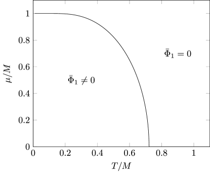
Figure 1: Phase diagram for the 2+1 dimensional Gross-Neveu model in chiral limit. The critical line separates two phases with nonzero and zero condensate.

In the case of graphene this phase transition is known as semimetal-insulator transition [28]. This transition has been widely studied by various methods e.g. Dyson-Schwinger method [29], Lattice simulation [30] etc. Even though there has been much theoretical studies to understand this transition, it is yet to be observed experimentally. The paper [31] attributed this inability to see this experiments on the screening of Coulomb interaction due to disorder, doping, thermal effect and volume effects which strongly suppresses the transition even in the very strong coupling regime.

Thermodynamical quantities like pressure and energy can be calculated from the grand canonical potential. For example, pressure per particle species $\mathcal{P}=-\Omega^{ren}/N-\mathcal{B}$. where the Bag term $\mathcal{B}$ is chosen to have zero pressure in the vacuum (zero temperature and zero chemical potential). The analytical expression for the pressure is given below in terms of the polylogarithm function.

$$\mathcal{P}(T,\mu)=\dfrac{M}{2\pi}\bar{\Phi}_{1}^{2}-\dfrac{\bar{\Phi}_{1}^{3}}{3\pi}-\dfrac{M^{3}}{6\pi}-\dfrac{1}{\pi\beta^{3}}\left[\beta\bar{\Phi}_{1}(\rm{Li}_{2}(-e^{-\beta(\bar{\Phi}_{1}-\mu)}))+\rm{Li}_{3}(-e^{-\beta(\bar{\Phi}_{1}-\mu)})+(\mu\to-\mu)\right].$$ (10)

where $\bar{\Phi}_{1}$ are calculated by solving the gap equation (8). Entropy and the Number density can be calculated from the relation $\mathcal{S}=\frac{\partial\mathcal{P}}{\partial T}$ and $\mathcal{N}=\frac{\partial\mathcal{P}}{\partial\mu}$. Using these we can also calculate the energy density

$$\mathcal{E}=-\mathcal{P}+T\mathcal{S}+\mu\mathcal{N}.$$ (11)

In figure 2 we have shown the speed of sound in the medium calculated from the relation $c_{s}^{2}=\frac{d\mathcal{P}}{d\mathcal{E}}$. The speed of sound squared correctly goes to the conformal limit $1/2$ for high temperature as can be seen from the figure.

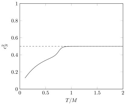
Figure 2: Speed of sound squared as a function of temperature. The dashed line shows the conformal limit $c_{s}^{2}=1/d$.

IV Beyond Mean Field

Mean field approximation replaces the auxiliary fields by their expectation values. In doing so it ignores the fluctuations effects of the auxiliary fields. In our method this can be done by adding perturbation to the mean fields $\bar{\Phi}_{i}\to\bar{\Phi}_{i}+\delta\Phi_{i}$. Substituting this into (3), inside the exponential we have the following terms,

$$-N\int d^{3}x\sum_{i=1}^{4}\left(\frac{\bar{\Phi}_{i}^{2}+\delta\Phi_{i}^{2}+2\bar{\Phi}_{i}\delta\Phi_{i}}{2G}-\delta_{k1}\kappa(\bar{\Phi}_{i}+\delta\Phi_{i})\right)+N\rm{Tr}\ln S_{\rm tot}^{-1}.$$ (12)

where $S_{\rm tot}^{-1}=S_{\rm mf}^{-1}+\Sigma$ with $\Sigma=\sum_{i=1}^{4}\Gamma_{i}\delta\Phi_{i}$. The trace log part can be split into

$$\rm{Tr}\ln(\beta S_{\rm tot}^{-1})=\rm{Tr}\ln(\beta S^{-1}_{\rm mf})+\rm{Tr}\ln(\beta(1+S_{mf}\Sigma)).$$ (13)

Now we can separate the mean field part as $\mathcal{Z}=\mathcal{Z}_{\rm mf}\mathcal{Z}_{\rm fl}$, with

$$\mathcal{Z}_{\rm fl}=\int\prod_{i=1}^{4}\mathcal{D}\delta\Phi_{i}\rm{exp}\left\{-N\int d^{3}x\sum_{i=1}^{4}\left(\frac{\delta\Phi_{i}^{2}+2\bar{\Phi}_{i}\delta\Phi_{i}}{2G}-\delta_{k1}\kappa\delta\Phi_{i}\right)+N\rm{Tr}\ln(1+S_{\rm mf}\Sigma)\right\}.$$ (14)

The last term can be approximated as $\rm{Tr}\ln(1+S_{\rm mf}\Sigma)\approx\rm Tr(S_{\rm mf}\Sigma)+\rm{Tr}(S_{\rm mf}\Sigma S_{\rm mf}\Sigma)$. All the linear term in field $\delta\Phi_{i}$ should vanish and we are left with,

$$\mathcal{Z}_{\rm fl}=\int\prod_{i=1}^{4}\mathcal{D}\delta\Phi_{i}\rm{exp}\left\{-\int d^{3}x\sum_{i=1}^{4}\frac{\delta\Phi_{i}^{2}}{2}\left(\frac{N}{G}-2N\rm{Tr}(S_{\rm mf}\Gamma_{i}S_{\rm mf}\Gamma_{i})\right)\right\}.$$ (15)

The second term inside the bracket looks similar to polarisation loop integral in path integral. We define $\Pi=2N\rm{Tr}(S_{\rm mf}\Gamma_{i}S_{\rm mf}\Gamma_{i})$. The expression of it is given below [20]

$$\Pi(q,\omega)=-N\sum_{s,s^{\prime}=\pm 1}\int\dfrac{d^{2}p}{(2\pi)^{2}}\dfrac{f^{-}(s^{\prime}E_{k})-f^{-}(sE_{p})}{\omega+s^{\prime}E_{k}-sE_{p}}\left(1-ss^{\prime}\dfrac{\vec{p}\cdot\vec{k}\mp m^{2}}{E_{p}E_{k}}\right).$$ (16)

where the negative sign corresponds to the fields $\Phi_{1,2}$ and the positive sign to the $\Phi_{3,4}$ and $\vec{k}=\vec{p}+\vec{q}$. Following the convention used in the NJL model, we will denote the fields $\Phi_{1,2}$ as scalar field $\sigma$ and $\Phi_{3,4}$ as the pseudo-scalar field $\varphi$. BY evaluating the gaussian integral we find the relation between polarisation function and the grand potential.

$$\Omega_{\text{fl}}(T,\mu)=\frac{1}{2\beta l^{2}}\sum_{i=1}^{4}\log\det\left(\beta\mathcal{D}^{-1}_{i}\right),\qquad\mathcal{D}^{-1}_{i}=\frac{N}{G}-\Pi_{i}.$$ (17)

Where for brevity, we write $\Pi_{\Phi_{i}}$ as $\Pi_{i}$ and so on.

Firstly, we will focus on the case $q=0$. In this particular case, we have significant simplifications of the expression.

$$\Pi_{i}(0,\omega)=-2N\int\dfrac{d^{2}p}{(2\pi)^{2}}[f^{-}(E_{p})-f^{-}(-E_{p})]\left[\dfrac{1}{\omega+2E_{p}}-\dfrac{1}{\omega-2E_{p}}\right]\begin{pmatrix}p^{2}/E_{p}^{2}\\ 1\end{pmatrix}.$$ (18)

Note that the upper term in the last bracket corresponds to the index $i=1,2$ i.e. for the scalar channel and the lower term corresponds to the pseudo-scalar. It is interesting that the renormalisation technique used at the mean-field level still works for this case.

Using the Plemj relation we obtain the imaginary part

$$\textrm{Im}[\Pi_{i}(0,\omega+i\eta)]=\dfrac{N}{4}\omega(f^{-}(\omega/2)-f^{-}(-\omega/2))\begin{pmatrix}(\omega^{2}-4m^{2})/\omega^{2}\\ 1\end{pmatrix}.$$ (19)

The real part can be calculated using either the Kramers-Kronig relation.

IV.1 Bound Excitonic States

Polarisation function at rest gives information about the bound excitonic states. The zeros of the spectral function $\mathcal{D}^{-1}$ at zero momentum correspond to the mass of such bound states.

$$\frac{N}{G}-\Pi_{i}(0,i\omega=M)=0.$$ (20)

The masses are shown in the figure 3. Scalar mass is slightly heavier than the twice of fermion mass for low temperatures which makes them unstable. The pseudo-scalar masses on the other hand is much lighter and stable. Note that the pseudo-scalar particle corresponds to the Goldstone boson of the system. In chiral limit ($m_{0}=0$) Goldstone mass should go to zero; In the figure 3 we show masses at some small value of $m_{0}$ ($\kappa=0.01$). The pseudo-scalar states becomes unbound at Mott temperature ($M_{\Phi_{3,4}}(T_{\rm Mott})=2\bar{\Phi_{1}}(T_{\rm Mott})$) and beyond.

In the case of Graphene, this Mott critically has been previously studied in [32, 33].

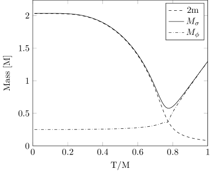
Figure 3: Masses of the bound excitonic states in the scalar (solid line) and pseudo-scalar (dash-dotted line) channels. The dashed line shows the twice of the condensate mass. The values are calculated at small bare mass correspondi

IV.2 Phase Shift and Beth-Uhlenbeck approach

As it has been figured out in [34] and outlined in greater detail in [35], the phase shift for fluctuations in the NJL model can be decomposed in a resonant part and a background contribution. Here, ee are following the paper [21] and decompose the polarisation function into two contributions

$$\Pi_{i}(q,\omega)=\Pi_{i,0}+\Pi_{i,2}(q,\omega),$$

where we have separated the momentum and frequency independent part $\Pi_{0}$ from the remainder $\Pi_{2}(q,\omega+i\eta)$

$$\mathcal{D}_{i}^{-1}(q,\omega+i\eta) =\dfrac{N}{G}-\Pi_{i,0}-\Pi_{i,2}(q,\omega+i\eta)$$

$$=\Pi_{i,2}(q,\omega+i\eta)(R_{i}(q,\omega^{2})-1),$$ (21)

with

$$R_{i}(q,\omega^{2})=\dfrac{\frac{N}{G}-\Pi_{i,0}}{\Pi_{i,2}(q,\omega+i\eta)}.$$ (22)

Introducing $R(q,\omega^{2})$ in such a way enables us to write,

$$\rm{Im}\log\mathcal{D}_{i}^{-1}(q,\omega+i\eta) = \text{Im}\log\Pi_{i,2}(q,\omega+i\eta)+\text{Im}\log[R_{i}(q,\omega^{2})-1]$$ (23)

$$\text{or,}\quad\phi(i,q,\omega) = \phi_{i,\rm sc}(q,\omega)+\phi_{i,\rm R}(q,\omega).$$ (24)

The phase is separated into two parts the scattering part and the resonant part

$$\phi_{i,sc}(q,\omega)=-\arctan\left(\dfrac{\rm{Im}\Pi_{i,2}(q,\omega+i\eta)}{\rm{Re}\Pi_{i,2}(q,\omega+i\eta)}\right).$$ (25)

$$\phi_{\Phi_{i},R}(q,\omega)=\arctan\left(\dfrac{\rm{Im}(R_{i}(q,\omega^{2}))}{1-\rm{Re}(R_{i}(q,\omega^{2}))}\right).$$ (26)

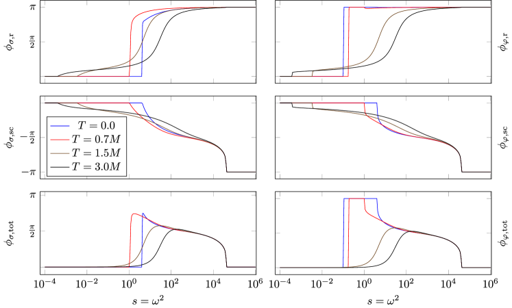
Figure 4: Phases for scalar(right) and pseudo scalar(left) channels. Resonant and the scattering part of the phase are shown in the top two rows and total phase is in the last row.

Phases at zero external momentum are shown in the figure 4. The resonant part changing from $0$ to $\pi$ hints at the presence of bound states. The figure is obtained by taking $\Lambda=100M$. The phases goes to zero beyond the cutoff frequency $\Lambda$. The form of the phase shift remain unchanged around the energy of the order $M$ as long as the $\Lambda\gg M$.

IV.2.1 Pressure

The pressure due to fluctuations from the mean field theory is given by the equation

$$\mathcal{P}_{\text{fl}}(T,\mu)=-\sum_{i=1}^{4}\int\dfrac{d^{2}q}{(2\pi)^{2}}\int_{-q^{2}}^{\infty}ds\left[\dfrac{1}{2}\sqrt{q^{2}+s}+\dfrac{1}{\beta}\log\left(1-e^{-\beta\sqrt{q^{2}+s}}\right)\right]D_{i}(s).$$ (27)

where $s=\omega^{2}-q^{2}$ and $D_{i}(s)=\dfrac{1}{\pi}\dfrac{d\phi_{i}(s)}{ds}$.

In the paper [21] phase shifts at non-zero external momentum are approximated via boost from the phase shifts at rest.

$$\mathcal{P}_{\text{fl}}(T,\mu)=-\sum_{i}\int\dfrac{d^{2}q}{(2\pi)^{2}}\int_{0}^{\infty}ds\left[\dfrac{1}{2}\sqrt{q^{2}+s}+\dfrac{1}{\beta}\log\left(1-e^{-\beta\sqrt{q^{2}+s}}\right)\right]D_{i}(s)\quad\text{with }s=\omega^{2}.$$ (28)

Note that the integral is divergent and can be made finite by subtracting the term with $T=0$ and $\mu=0$. Clearly the first term in the integral is temperature independent and would drop out, resulting in the non-divergent integral

$$\mathcal{P}_{\text{fl}}(T,\mu)=-\sum_{i}\int\dfrac{d^{2}q}{(2\pi)^{2}}\int_{0}^{\infty}ds\dfrac{1}{\beta}\log\left(1-e^{-\beta\sqrt{q^{2}+s}}\right)D_{i}(s)\quad\text{with }s=\omega^{2}.$$ (29)

This integral can be done numerically but as the derivative of phase is not very smooth function of $s$ (resembles Dirac Delta function), it is easier to do the integral if we use integration by parts first.

$$\mathcal{P}_{\text{fl}}(T,\mu) =\sum_{i}\int\dfrac{d^{2}q}{(2\pi)^{2}}\int_{0}^{\infty}ds\dfrac{e^{-\beta\sqrt{q^{2}+s}}}{2\sqrt{q^{2}+s}\left(1-e^{-\beta\sqrt{q^{2}+s}}\right)}\dfrac{\phi_{i}(0,s)}{\pi}\quad\text{with }s=\omega^{2},$$ (30)

$$=\sum_{i}\int_{0}^{\infty}\dfrac{ds}{4\pi^{2}}\phi_{i}(0,s)\left(-\sqrt{s}+\dfrac{1}{\beta}\log\left(1-e^{-\beta\sqrt{s}}\right)\right).$$ (31)

Dividing the phase into the resonant and scattering parts, correspondingly we can obtain the resonant and scattering parts of the pressure as well. The figure 5 shows the pressures for both $\varphi$ and $\sigma$. It is interesting to note that the fluctuation-induced pressure does not vanish even at temperatures several times higher than the typical scale of $M$. This can be explained by the fact that the cutoff in this case is much larger than $M$. The phase shifts approach zero near the cutoff scale, and since the factor multiplying the phase shifts in the pressure calculation only has significant values around $T$, the temperature must be on the order of the cutoff for the pressure to effectively approach zero.

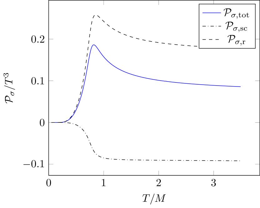
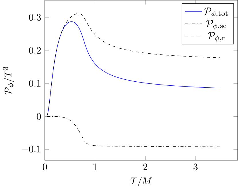
Figure 5: First order correction to the pressure due to fluctuations for scalar (left) and pseudo-scalar (right) channels. The blue solid line corresponds to the total pressure while the dashed and dash-dotted lines corresponds to the resonant part and the scattering part respectively.

IV.2.2 Pole Approximation

In the paper [20] the authors have used a pole approximation to model the phase shifts. Here we present a brief comparison of the pole approximation with the exact phase shifts. The approximation was carried out by assuming

$$D_{i}(s)\approx\pi\delta\left(\omega-\sqrt{q^{2}+M_{\Phi_{i}}^{2}}\right).$$ (32)

Substituting this into the equation (27) we obtain the pressure due to fluctuation as shown in the figure 6 along with the pressure calculated without the approximation. The simple pole approximation managed to capture the resonant part of the pressure at low temperature, but fails in the high temperature limit.

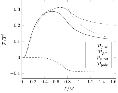
Figure 6: Comparing the pressure due to pole approximation with the computed pressure with full phase calculation at zero momentum.

IV.3 Effect of Finite Momenta

In the previous section we approximated the momentum dependence of the phase shifts by boosting the values calculated at zero external momenta, $\phi(q,\omega)\approx\phi(q=0,s=\sqrt{\omega^{2}-q^{2}})$. In this section, we numerically explore the momentum dependence. In Appendix C we present the analytical expressions for the imaginary part of the polarisation function. Real part can be calculated from Kramers-Kronig relation. Phases are then obtained using (25) and (26) and are shown in the figure 7. Phase shifts are very similar for $s>4m^{2}$ and the main difference is in the region $s<4m^{2}$. Note that as per the equation for pressure (27) the phase shifts are weighed by a factor which is exponentially suppressed for large $s$. Hence this seemingly minute difference in the phase shifts at low $s$ will have a significant effect on the pressure. Similar calculations for the case of the NJL model coupled with Polyakov loop can be found in [36].

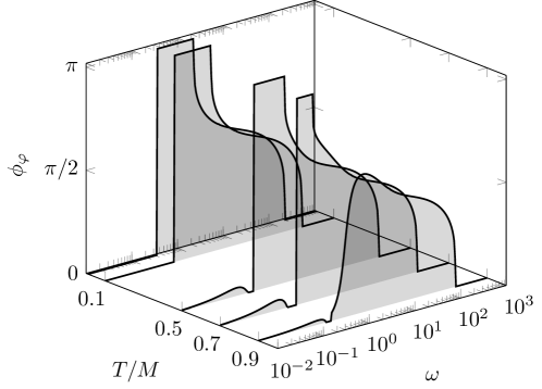
Figure 7: Phase shifts for the pseudo-scalar channel at external momentum $q=0.3M$, shown at various temperatures.

V Conclusions

In this article, we have explored a graphene-inspired generalized Gross-Neveu model in $2+1$ dimensions. In the mean field level, the model shows a second order transition from semimetal to insulator. As detailed in Appendix B, there is instability in the point $T=0,\mu=M$. This instabilty gets enhanced when the theory is coupled to external magnetic field [37]. When compared to its 3D counterpart of the model, the thermodynamical quantities at the mean field have different scale dependence on temperature and chemical potential but shows similar trend when normalised appropriately. Beyond mean field also the bound state spectra and the phase shifts follow similar pattern to the corresponding 3D version. While the difference lies in the extent of renormalisibility. It shows up in many way from having less dependence on the cutoff to having speed of sound being subluminal. Finally, we present finite momentum dependent phase shifts. Here we ellude to the difference between the existing method of using boosts from the phase shifts at rest and the full momentum dependent calculations. The actual difference and how it effects the fluctuation pressure etc. will be of particular importance and are delegated to the forthcoming publication.

Appendix A Gamma Matrices

Representation of gamma matrices used in this text,

$$\gamma_{k}=\begin{pmatrix}0&i\tau_{k}\\ -i\tau_{k}&0\end{pmatrix}\text{,}\qquad\gamma_{3}=\begin{pmatrix}0&I_{2}\\ I_{2}&0\end{pmatrix},$$

There exist two other 2 by 2 matrices which anticommutes with the above three,

$$\gamma_{4}=\begin{pmatrix}0&i\tau_{3}\\ -i\tau_{3}&0\end{pmatrix}\text{,}\qquad\gamma_{5}=\gamma_{1}\gamma_{2}\gamma_{3}\gamma_{4}=\begin{pmatrix}I_{2}&0\\ 0&I_{2}\end{pmatrix}.$$ (33)

$\gamma_{45}$ which commutes with $\gamma_{\mu}$ but anti-comutes with $\gamma_{4}$ and $\gamma_{5}$ is then defined by

$$\gamma_{45}=\frac{i}{2}[\gamma_{4},\gamma_{5}]=\begin{pmatrix}0&\tau_{3}\\ \tau_{3}&0\end{pmatrix}$$ (34)

Appendix B Order of Phase Transition

To gain insight about the order of the phase transition, it is worth looking at the grand potential as a function of the order parameter $\bar{\Phi}_{1}$. It is W (Mexican hat) shaped inside the enclosed area (by critical line and the axes) in Fig. 1. The minima is located at a finite value of $\bar{\Phi}_{1}$ indicating chiral symmetry breaking. On the other hand, in the outside region the potential is U-shaped with minima at zero, restoring the chiral symmetry. The case of zero temperature is slightly different. The zero temperature limit for the grand potential can be obtained by using the following identity (35) in equation (5).

$$\lim_{\beta\to\infty}\log\left(1+e^{\beta x}\right)=x\theta(x),$$ (35)

$$\Omega(T\to 0,\mu)/N=\frac{\bar{\Phi}_{1}^{2}}{2g}+\frac{M^{3}}{3\pi}-\sum_{k=1}^{2}\int\frac{d^{2}p}{(2\pi)^{2}}(\mu-E_{p}^{(k)})\theta(\mu-E_{p}^{(k)}).$$ (36)

which simplifies to,

$$\Omega(T\to 0,\mu)/N=\begin{cases}\frac{\bar{\Phi}_{1}^{2}}{2g}+\frac{|\bar{\Phi}_{1}|^{3}}{3\pi},&\bar{\Phi}_{1}>\mu\\ -\frac{\bar{\Phi}_{1}^{2}}{2\pi}\left(\frac{\pi}{-g}-\mu\right)-\frac{\mu^{3}}{6\pi},&\bar{\Phi}_{1}<\mu.\end{cases}$$ (37)

At $\mu=\frac{\pi}{-g}=M$ the grand potential admits minima for a wide range of $\bar{\Phi}_{1}$ values (between $0$ and $M$). A similar result is obtained in [37].

Appendix C External momentum dependence of the Polarisation

To calculate the imaginary part of the polarisation function with non-zero external momentum we use the Sokhotski–Plemelj relation in (16) to obtain the following expression.

$$\textrm{Im}[\Pi(q,\omega+i\eta)]=-2N\sum_{\xi,\xi^{\prime}=\pm 1}\int\dfrac{d^{2}p}{(2\pi)^{2}}(f^{-}(\xi^{\prime}E_{k})-f^{-}(\xi E_{p}))(-\pi)\delta(\omega+\xi^{\prime}E_{k}-\xi E_{p})\mathcal{T}^{\mp}_{\xi\xi^{\prime}}.$$ (38)

where $\mathcal{T}^{\mp}_{\xi,\xi^{\prime}}=\left(1-\xi\xi^{\prime}\frac{\vec{p}\cdot\vec{k}\mp m^{2}}{E_{p}E_{k}}\right)$ which can be simplified by assuming the constraint of the delta function, $\mathcal{T}^{\mp}_{\xi\xi^{\prime}}=\frac{-\xi\xi^{\prime}}{2E_{p}E_{k}}(\omega^{2}-q^{2}-\psi_{\mp})$ with $\psi_{+}=0$ and $\psi_{-}=4m^{2}$. With this, the imaginary part has the following form.

$$\textrm{Im}[\Pi(q,\omega+i\eta)]=N(s-\psi_{\mp})\left[-\theta(-s)\int_{y}^{\sqrt{\Lambda^{2}+\bar{\Phi}_{1}^{2}}}dx\frac{B_{1}(x)}{F(x)}+\theta(s-4m^{2})\int_{-y}^{y}dx\frac{B_{2}(x)}{F(x)}\right].$$ (39)

where the Pauli blocking factors are,

$$B_{2}(x)=f^{-}\left(\frac{-x-\omega}{2}\right)-f^{-}\left(\frac{-x+\omega}{2}\right),\qquad B_{1}(x)=B_{2}(x)+B_{2}(-x),$$ (40)

factor in the denominator

$$F(x)=4\pi\sqrt{q^{2}(s-4m^{2})-sx^{2}},$$ (41)

and $y=q\sqrt{1-4m^{2}/s}$.

The real part can be calculated using the Kramers-Kronig relation.

$$\textrm{Re}[\Pi(q,\omega)]=\dfrac{1}{\pi}\mathchoice{{\vbox{\hbox{$\textstyle-$}}\kern-4.86108pt}}{{\vbox{\hbox{$\scriptstyle-$}}\kern-3.25pt}}{{\vbox{\hbox{$\scriptscriptstyle-$}}\kern-2.29166pt}}{{\vbox{\hbox{$\scriptscriptstyle-$}}\kern-1.875pt}}\!\int\dfrac{d\omega^{\prime}}{\omega-\omega^{\prime}}\textrm{Im}[\Pi(q,\omega^{\prime})].$$ (42)

References

- Novoselov et al. [2005] K. S. Novoselov, A. K. Geim, S. V. Morozov, D. Jiang, M. I. Katsnelson, I. V. Grigorieva, S. V. Dubonos, and A. A. Firsov, Nature 438, 197 (2005), number: 7065 Publisher: Nature Publishing Group.
- Castro Neto et al. [2009] A. H. Castro Neto, F. Guinea, N. M. Peres, K. S. Novoselov, and A. K. Geim, Reviews of Modern Physics 81, 109 (2009), _eprint: 0709.1163.
- González [2010] J. González, Physical Review B - Condensed Matter and Materials Physics 82, 1 (2010).
- Hofmann et al. [2014] J. Hofmann, E. Barnes, and S. Das Sarma, Physical Review Letters 113, 1 (2014), _eprint: 1405.7036.
- Gross and Neveu [1974] D. J. Gross and A. Neveu, Physical Review D 10, 3235 (1974), publisher: American Physical Society.
- Barducci et al. [1995] A. Barducci, R. Casalbuoni, R. Gatto, M. Modugno, and G. Pettini, Physical Review D 51, 3042 (1995), arXiv:hep-th/9406117.
- Thies and Urlichs [2003] M. Thies and K. Urlichs, Physical Review D 67, 125015 (2003).
- Ciccone et al. [2022] R. Ciccone, L. Di Pietro, and M. Serone, Physical Review Letters 129, 071603 (2022), publisher: American Physical Society.
- Nambu and Jona-Lasinio [1961] Y. Nambu and G. Jona-Lasinio, Physical Review 122, 345 (1961), publisher: American Physical Society.
- Eguchi [1976] T. Eguchi, Physical Review D 14, 2755 (1976), publisher: American Physical Society.
- Kikkawa [1976] K. Kikkawa, Progress of Theoretical Physics 56, 947 (1976).
- Volkov [1984] M. K. Volkov, Annals of Physics 157, 282 (1984).
- Hatsuda and Kunihiro [1985] T. Hatsuda and T. Kunihiro, Physical Review Letters 55, 158 (1985), publisher: American Physical Society.
- Hatsuda and Kunihiro [1984] T. Hatsuda and T. Kunihiro, Physics Letters B 145, 7 (1984).
- Fukushima [2004] K. Fukushima, Physics Letters B 591, 277 (2004).
- Ratti et al. [2006] C. Ratti, M. A. Thaler, and W. Weise, Phys. Rev. D 73, 014019 (2006), arXiv:hep-ph/0506234 .
- Hansen et al. [2020] H. Hansen, R. Stiele, and P. Costa, Physical Review D 101, 094001 (2020), publisher: American Physical Society.
- Ebert et al. [2016] D. Ebert, K. G. Klimenko, P. B. Kolmakov, and V. C. Zhukovsky, Annals of Physics 371, 254 (2016), arXiv:1509.08093 [cond-mat, physics:hep-th].
- Zhukovsky and Klimenko [2015] V. C. Zhukovsky and K. G. Klimenko, Moscow University Physics Bulletin 70, 466 (2015).
- Ebert and Blaschke [2019] D. Ebert and D. Blaschke, Progress of Theoretical and Experimental Physics 2019, 123I01 (2019).
- Blaschke et al. [2014] D. Blaschke, M. Buballa, A. Dubinin, G. Röpke, and D. Zablocki, Annals of Physics 348, 228 (2014).
- Note [1] Representation of the gamma matrices can be found in the appendix A.
- Gusynin et al. [2007] V. P. Gusynin, S. G. Sharapov, and J. P. Carbotte, International Journal of Modern Physics B 21, 4611 (2007), arXiv:0706.3016 [cond-mat, physics:hep-ph].
- Rosenstein et al. [1989] B. Rosenstein, B. J. Warr, and S. H. Park, Physical Review Letters 62, 1433 (1989), publisher: American Physical Society.
- Erramilli et al. [2023] R. S. Erramilli, L. V. Iliesiu, P. Kravchuk, A. Liu, D. Poland, and D. Simmons-Duffin, Journal of High Energy Physics 2023, 36 (2023), arXiv:2210.02492 [cond-mat, physics:hep-lat, physics:hep-th].
- Mihaila et al. [2017] L. N. Mihaila, N. Zerf, B. Ihrig, I. F. Herbut, and M. M. Scherer, Physical Review B 96, 1 (2017), _eprint: 1703.08801.
- Parazian [2024] V. V. Parazian, Physics Letters A 510, 129544 (2024).
- Juricic et al. [2009] V. Juricic, I. F. Herbut, and G. W. Semenoff, Phys. Rev. B 80, 081405 (2009), _eprint: 0906.3513.
- Khveshchenko and Shively [2006] D. V. Khveshchenko and W. F. Shively, Physical Review B 73, 115104 (2006), publisher: American Physical Society.
- Drut and Lähde [2009] J. E. Drut and T. A. Lähde, Physical Review B 79, 165425 (2009), publisher: American Physical Society.
- Liu et al. [2009] G.-Z. Liu, W. Li, and G. Cheng, Physical Review B 79, 205429 (2009), publisher: American Physical Society.
- Herbut et al. [2009] I. F. Herbut, V. Juričić, and O. Vafek, Physical Review B 80, 075432 (2009).
- Classen et al. [2015] L. Classen, I. F. Herbut, L. Janssen, and M. M. Scherer, Physical Review B 92, 035429 (2015), publisher: American Physical Society.
- Hufner et al. [1994] J. Hufner, S. Klevansky, P. Zhuang, and H. Voss, Annals of Physics 234, 225 (1994).
- Wergieluk et al. [2013] A. Wergieluk, D. Blaschke, Y. L. Kalinovsky, and A. Friesen, Phys. Part. Nucl. Lett. 10, 660 (2013), arXiv:1212.5245 [nucl-th] .
- Maslov and Blaschke [2023] K. Maslov and D. Blaschke, Effect of mesonic off-shell correlations in the PNJL equation of state (2023), arXiv:2301.09882 [hep-ph, physics:nucl-th].
- Lenz et al. [2023] J. J. Lenz, M. Mandl, and A. Wipf, Physical Review D 108, 074508 (2023).