What we can learn from the angular differential rates (only) in semileptonic $B\to D^{*}\ell\nu_{\ell}$ decays

Abstract

We present a new, simple approach to the study of semileptonic $B\to D^{*}\ell\nu_{\ell}$ decays based on the angular distributions of the final state particles only. Our approach is model independent and never requires the knowledge of $|V_{cb}|$. By studying such distributions in the case of light leptons, a comparison between results from different data sets from the Belle and BelleII Collaborations and between data and Standard Model calculations is also given for several interesting quantities. A good consistency is observed between some of the experimental results and the theoretical predictions.

I Introduction

In this paper we introduce a new, straightforward approach to the analysis of semileptonic $B\to D^{*}\ell\nu_{\ell}$ decays based on the angular distributions of the final state particles. Although several analyses which make use the angular distributions already exist in the literature Tanaka:2012nw ; Sakaki:2013bfa ; Duraisamy:2013pia ; Ivanov:2016qtw ; Colangelo:2018cnj ; Bigi:2017njr ; Jung:2018lfu ; Jaiswal:2020wer ; Bordone:2024weh , our study is original in that it is only based on the angular distributions and it reduces the problem to the determination of few basic parameters (five in all). These parameters encode in the most general way the contributions to the differential decay rates coming from operators present in the effective Hamiltonian either in the Standard Model (SM) or from physics Beyond the Standard Model (BSM). The analysis is model independent and never requires the knowledge of $|V_{cb}|$. Thus, it allows a direct comparison of results obtained from different experimental data set as well as with the theoretical predictions based on the hadronic form factors (FFs) obtained from Lattice QCD (LQCD). While in some specific cases differences (within about two standard deviations) are visible, a quite good consistency is observed between some of the experimental results and the theoretical predictions of the SM using the LQCD FFs. The present study is limited to $B\to D^{*}\ell\nu_{\ell}$ decays with light leptons in the final states, for which possible BSM contributions have been considered in the past Bernlochner:2014ova ; Jung:2018lfu ; Fedele:2023ewe ; Colangelo:2024mxe .

Using the most general structure of the four-fold differential decay rate for semileptonic $B\to D^{*}\ell\nu_{\ell}$ decays, the five basic parameters (denoted in the following as $\{\eta,\eta^{\prime},\delta,\epsilon,\epsilon^{\prime}\}$) are defined in terms of experimentally measurable quantities related to different angular distributions, which will be the basis of our phenomenological analysis, namely

$$\frac{1}{\Gamma}\frac{d\Gamma}{d\mbox{cos}\theta_{v}} = \frac{3}{4(1+\eta)}\left\{\eta+(2-\eta)\mbox{cos}^{2}\theta_{v}\right\}~{},~{}$$ (1)

$$\frac{1}{\Gamma}\frac{d\Gamma}{d\mbox{cos}\theta_{\ell}} = \frac{3}{8(1+\eta^{\prime})}\left\{2+\eta^{\prime}-2\delta\mbox{cos}\theta_{\ell}-(2-\eta^{\prime})\mbox{cos}^{2}\theta_{\ell}\right\}~{},~{}$$ (2)

$$\frac{1}{\Gamma}\frac{d\Gamma}{d\chi} = \frac{1}{2\pi}\left\{1-\frac{\epsilon}{1+\eta}\mbox{cos}2\chi-\frac{\epsilon^{\prime}}{1+\eta}\mbox{sin}2\chi\right\}~{}.~{}$$ (3)

In order to disentangle $\delta$ from $\eta^{\prime}$, a separation of the dependence of $1/\Gamma d\Gamma/d\mbox{cos}\theta_{\ell}$ on the even or odd terms in $\mbox{cos}\theta_{\ell}$ is necessary. In literature it is common to refer to observables like the forward-backward asymmetry $A_{FB}$, the longitudinal $D^{*}$-polarization fraction $F_{L}$, and the two transverse asymmetries $A_{1c}$ and $A_{9c}$ . These quantities are related to the five hadronic parameters $\{\eta,\eta^{\prime},\delta,\epsilon,\epsilon^{\prime}\}$ by

$$A_{FB} = -\frac{3}{4}\frac{\delta}{1+\eta^{\prime}}~{},~{}$$ (4)

$$F_{L} = \frac{1}{1+\eta}~{},~{}$$ (5)

$$A_{1c} = -\frac{\epsilon}{1+\eta}~{},~{}$$ (6)

$$A_{9c} = -\frac{\epsilon^{\prime}}{1+\eta}~{},~{}$$ (7)

and will be used in the present analysis.

The plan of the remainder of the paper is the following: in Sec. II we recall the most general expression of the $B\to D^{*}$ differential decay rate in the momentum transfer and in the relevant angular variables. We then derive the expressions given in Eqs. (1)-(7); in Sec. III we express the basic parameters $\{\eta,\eta^{\prime},\delta,\epsilon,\epsilon^{\prime}\}$ in terms of the helicity amplitudes computed in the SM; in Sec. IV we describe our fit of the data from different measurements, present tables and figures containing the results and discuss their compatibility and consistency with the SM. The final Section contains our conclusions.

II The four-fold $B\to D^{*}$ differential decay rate and the definition of the basic parameters

In this section we derive the expressions in Eqs. (1)-(3) from the four-fold $B\to D^{*}$ differential decay rate.

The general structure of the four-fold differential rate for $B\to D^{*}\ell\nu_{\ell}$ decays, valid both within the SM and including possible BSM effects, can be expressed in terms of twelve angular observables (coefficients) $J_{i}(w)$ Duraisamy:2013pia ; Bernlochner:2014ova ; Ivanov:2016qtw ; Belle:2023xgj , functions of the recoil variable $w$, which is given in terms of the squared four-momentum transfer $q^{2}$ by

$$w\equiv\frac{1+r^{2}-q^{2}/m_{B}^{2}}{2r}~{}\,$$ (8)

with $r\equiv m_{D^{*}}/m_{B}$. The dependence on the squared momentum transfer is all condensed in the angular observables themselves, which can be expressed in terms of the helicity amplitudes (and then in terms of the hadronic FFs) and of the Wilson coefficients of the relevant operators as done in Refs. Duraisamy:2013pia ; Ivanov:2016qtw (very detailed and complementary discussions can be also found in Refs. Tanaka:2012nw ; Colangelo:2018cnj ). The physical quantities $J_{i}(w)$ are particularly relevant to scrutinize the presence of BSM effects in semileptonic $B\to D^{*}$ decays. Following the notation of Ref. Belle:2023xgj one has

$$\frac{d^{4}\Gamma(B\to D^{*}\ell\nu_{\ell})}{dwd\mbox{cos}\theta_{v}d\mbox{cos}\theta_{\ell}d\chi} = \frac{3}{16\pi}\Gamma_{0}\left\{J_{1s}(w)\mbox{sin}^{2}\theta_{v}+J_{1c}(w)\mbox{cos}^{2}\theta_{v}\right.$$

$$+ \left.J_{2s}(w)\mbox{sin}^{2}\theta_{v}\mbox{cos}2\theta_{\ell}+J_{2c}(w)\mbox{cos}^{2}\theta_{v}\mbox{cos}2\theta_{\ell}\right.$$

$$+ \left.J_{3}(w)\mbox{sin}^{2}\theta_{v}\mbox{sin}^{2}\theta_{\ell}\mbox{cos}2\chi+J_{4}(w)\mbox{sin}2\theta_{v}\mbox{sin}2\theta_{\ell}\mbox{cos}\chi\right.$$

$$+ \left.J_{5}(w)\mbox{sin}2\theta_{v}\mbox{sin}\theta_{\ell}\mbox{cos}\chi+J_{6s}(w)\mbox{sin}^{2}\theta_{v}\mbox{cos}\theta_{\ell}\right.$$

$$+ \left.J_{6c}(w)\mbox{cos}^{2}\theta_{v}\mbox{cos}\theta_{\ell}+J_{7}(w)\mbox{sin}2\theta_{v}\mbox{sin}\theta_{\ell}\mbox{sin}\chi\right.$$

$$+ \left.J_{8}(w)\mbox{sin}2\theta_{v}\mbox{sin}2\theta_{\ell}\mbox{sin}\chi+J_{9}(w)\mbox{sin}^{2}\theta_{v}\mbox{sin}^{2}\theta_{\ell}\mbox{sin}2\chi\right\}~{},~{}$$

where

$$\Gamma_{0}\equiv\frac{\eta_{EW}^{2}m_{B}m_{D^{*}}^{2}}{(4\pi)^{3}}G_{F}^{2}|V_{cb}|^{2}$$ (10)

with $\eta_{EW}=1.0066$, $G_{F}$ the Fermi constant and $V_{cb}$ the relevant CKM matrix element. The angles $\theta_{v}$, $\theta_{\ell}$ and $\chi$ are defined as in Fig. 1.

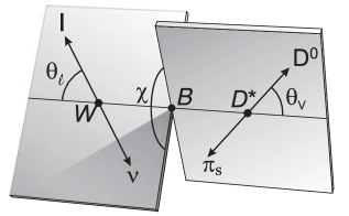
Figure 1: Definition of the angles $\theta_{v}$, $\theta_{\ell}$ and $\chi$ for the decay $B\to D^{*}(D\pi)\ell\nu_{\ell}$. This figure has been taken from Ref. Belle:2018ezy .

The total decay rate is given by

$$\Gamma(B\to D^{*}\ell\nu_{\ell})=\frac{2}{3}\Gamma_{0}\left[6\overline{J}_{1s}+3\overline{J}_{1c}-2\overline{J}_{2s}-\overline{J}_{2c}\right]~{},$$ (11)

where the quantities $\overline{J}_{i}$ are the integrated angular coefficients over the full kinematical range of $w$, namely

$$\overline{J}_{i}\equiv\int_{1}^{w_{max}^{\ell}}dwJ_{i}(w)$$ (12)

with

$$w_{max}^{\ell}\equiv\frac{1+r^{2}-m_{\ell}^{2}/m_{B}^{2}}{2r}~{}.~{}$$ (13)

By dividing Eq. (II) by the total rate $\Gamma$ one gets the four-fold decay ratio independent of $V_{cb}$, namely

$$\frac{1}{\Gamma}\frac{d^{4}\Gamma(B\to D^{*}\ell\nu_{\ell})}{dwd\mbox{cos}\theta_{v}d\mbox{cos}\theta_{\ell}d\chi} = \frac{1}{{\cal{N}}}\left\{J_{1s}(w)\mbox{sin}^{2}\theta_{v}+J_{1c}(w)\mbox{cos}^{2}\theta_{v}\right.$$

$$+ \left.J_{2s}(w)\mbox{sin}^{2}\theta_{v}\mbox{cos}2\theta_{\ell}+J_{2c}(w)\mbox{cos}^{2}\theta_{v}\mbox{cos}2\theta_{\ell}\right.$$

$$+ \left.J_{3}(w)\mbox{sin}^{2}\theta_{v}\mbox{sin}^{2}\theta_{\ell}\mbox{cos}2\chi+J_{4}(w)\mbox{sin}2\theta_{v}\mbox{sin}2\theta_{\ell}\mbox{cos}\chi\right.$$

$$+ \left.J_{5}(w)\mbox{sin}2\theta_{v}\mbox{sin}\theta_{\ell}\mbox{cos}\chi+J_{6s}(w)\mbox{sin}^{2}\theta_{v}\mbox{cos}\theta_{\ell}\right.$$

$$+ \left.J_{6c}(w)\mbox{cos}^{2}\theta_{v}\mbox{cos}\theta_{\ell}+J_{7}(w)\mbox{sin}2\theta_{v}\mbox{sin}\theta_{\ell}\mbox{sin}\chi\right.$$

$$+ \left.J_{8}(w)\mbox{sin}2\theta_{v}\mbox{sin}2\theta_{\ell}\mbox{sin}\chi+J_{9}(w)\mbox{sin}^{2}\theta_{v}\mbox{sin}^{2}\theta_{\ell}\mbox{sin}2\chi\right\}~{},~{}$$

where

$${\cal{N}}=\frac{8\pi}{9}\left[6\overline{J}_{1s}+3\overline{J}_{1c}-2\overline{J}_{2s}-\overline{J}_{2c}\right]~{}.~{}$$ (15)

After integrating Eq. (II) over the recoil variable $w$ and over two out of the three angular coordinates $\{\theta_{v},\theta_{\ell},\chi\}$ we obtain the single-differential angular decay rates

$$\frac{1}{\Gamma}\frac{d\Gamma}{d\mbox{cos}\theta_{v}} = \frac{4\pi}{3{\cal{N}}}\left\{3\overline{J}_{1s}-\overline{J}_{2s}\right.$$ (16)

$$+ \left.\left(3\overline{J}_{1c}-\overline{J}_{2c}-3\overline{J}_{1s}+\overline{J}_{2s}\right)\mbox{cos}^{2}\theta_{v}\right\}~{},~{}$$

$$\frac{1}{\Gamma}\frac{d\Gamma}{d\mbox{cos}\theta_{\ell}} = \frac{4\pi}{3{\cal{N}}}\left\{2\overline{J}_{1s}-2\overline{J}_{2s}+\overline{J}_{1c}-\overline{J}_{2c}\right.$$ (17)

$$+ \left.\left(2\overline{J}_{6s}+\overline{J}_{6c}\right)\mbox{cos}\theta_{\ell}+2\left(2\overline{J}_{2s}+\overline{J}_{2c}\right)\mbox{cos}^{2}\theta_{\ell}\right\}~{},~{}$$

$$\frac{1}{\Gamma}\frac{d\Gamma}{d\chi} = \frac{1}{2\pi}\left\{1+\frac{32\pi}{9{\cal{N}}}\overline{J}_{3}\mbox{cos}2\chi+\frac{32\pi}{9{\cal{N}}}\overline{J}_{9}\mbox{sin}2\chi\right\}~{}.~{}$$ (18)

By defining the following dimensionless quantities

$$\eta \equiv 2\frac{3\overline{J}_{1s}-\overline{J}_{2s}}{3\overline{J}_{1c}-\overline{J}_{2c}}~{},~{}$$ (19)

$$\eta^{\prime} \equiv 2\frac{2\overline{J}_{1s}+\overline{J}_{1c}+2\overline{J}_{2s}+\overline{J}_{2c}}{2\overline{J}_{1s}+\overline{J}_{1c}-3\left(2\overline{J}_{2s}+\overline{J}_{2c}\right)}~{},~{}$$ (20)

$$\delta = -2\frac{2\overline{J}_{6s}+\overline{J}_{6c}}{2\overline{J}_{1s}+\overline{J}_{1c}-3\left(2\overline{J}_{2s}+\overline{J}_{2c}\right)}~{},~{}$$ (21)

$$\epsilon \equiv -4\frac{\overline{J}_{3}}{3\overline{J}_{1c}-\overline{J}_{2c}}~{},~{}$$ (22)

$$\epsilon^{\prime} \equiv -4\frac{\overline{J}_{9}}{3\overline{J}_{1c}-\overline{J}_{2c}}~{},~{}$$ (23)

we get the expressions in Eqs. (1)-(3).

Therefore, even including BSM effects, the single-differential angular decay rates (1)-(3) have a precise dependence on the angular coordinates $\{\theta_{v},\theta_{\ell},\chi\}$ governed only by five hadronic parameters given by $\{\eta,\eta^{\prime},\delta,\epsilon,\epsilon^{\prime}\}$, defined by Eqs. (19)-(23) in terms of the integrated angular coefficients $\overline{J}_{i}$.

The quantities $A_{FB}$, $F_{L}$, $A_{1c}$ and $A_{9c}$ can be easily derived from Eqs. (1)-(3) obtaining Eqs. (4)-(7).

III The angular variables $J_{i}(w)$ in the SM

Within the SM the angular coefficients $J_{i}(w)$ can be expressed in terms of the helicity amplitudes $H_{+,-,0,t}(w)$ Belle:2023xgj as

$$J_{1s}(w) = \frac{3}{2}F(w)\left[H_{+}^{2}(w)+H_{-}^{2}(w)\right]\left(1+\frac{m_{\ell}^{2}}{3q^{2}}\right)~{},~{}$$ (24)

$$J_{1c}(w) = 2F(w)\left[H_{0}^{2}(w)\left(1+\frac{m_{\ell}^{2}}{q^{2}}\right)+2\frac{m_{\ell}^{2}}{q^{2}}H_{t}^{2}(w)\right]~{},~{}$$ (25)

$$J_{2s}(w) = \frac{1}{2}F(w)\left[H_{+}^{2}(w)+H_{-}^{2}(w)\right]\left(1-\frac{m_{\ell}^{2}}{q^{2}}\right)~{},~{}$$ (26)

$$J_{2c}(w) = -2F(w)H_{0}^{2}(w)\left(1-\frac{m_{\ell}^{2}}{q^{2}}\right)~{},~{}$$ (27)

$$J_{3}(w) = -2F(w)H_{+}(w)H_{-}(w)\left(1-\frac{m_{\ell}^{2}}{q^{2}}\right)~{},~{}$$ (28)

$$J_{4}(w) = F(w)H_{0}(w)\left[H_{+}(w)+H_{-}(w)\right]\left(1-\frac{m_{\ell}^{2}}{q^{2}}\right)~{},~{}$$ (29)

$$J_{5}(w) = 2F(w)\left\{H_{0}(w)\left[H_{-}(w)-H_{+}(w)\right]+\frac{m_{\ell}^{2}}{q^{2}}H_{t}(w)\left[H_{+}(w)+H_{-}(w)\right]\right\}~{},~{}\quad$$ (30)

$$J_{6s}(w) = -2F(w)\left[H_{+}^{2}(w)-H_{-}^{2}(w)\right]~{},~{}$$ (31)

$$J_{6c}(w) = -8\frac{m_{\ell}^{2}}{q^{2}}F(w)H_{0}(w)H_{t}(w)~{},~{}$$ (32)

$$J_{7}(w) = J_{8}(w)=J_{9}(w)=0~{},~{}$$ (33)

where the kinematical factor $F(w)$ is given by

$$F(w)\equiv\sqrt{w^{2}-1}~{}\left(1+r^{2}-2rw\right)~{}\left(1-\frac{m_{\ell}^{2}}{q^{2}}\right)^{2}~{}.~{}$$ (34)

It follows that, within the SM, the quantities $\{\eta,\eta^{\prime},\delta,\epsilon,\epsilon^{\prime}\}$ are explicitly given by

$$\eta = \frac{H_{++}+H_{--}+\frac{m_{\ell}^{2}}{2m_{B}^{2}}\left(\widetilde{H}_{++}+\widetilde{H}_{--}\right)}{H_{00}+\frac{m_{\ell}^{2}}{2m_{B}^{2}}\left(\widetilde{H}_{00}+3\widetilde{H}_{tt}\right)}~{},~{}$$ (35)

$$\eta^{\prime} = \frac{H_{++}+H_{--}+\frac{m_{\ell}^{2}}{m_{B}^{2}}\left(\widetilde{H}_{00}+\widetilde{H}_{tt}\right)}{H_{00}+\frac{m_{\ell}^{2}}{2m_{B}^{2}}\left(\widetilde{H}_{++}+\widetilde{H}_{--}-\widetilde{H}_{00}+\widetilde{H}_{tt}\right)}~{},~{}$$ (36)

$$\delta = \frac{H_{++}-H_{--}+\frac{2m_{\ell}^{2}}{m_{B}^{2}}\widetilde{H}_{0t}}{H_{00}+\frac{m_{\ell}^{2}}{2m_{B}^{2}}\left(\widetilde{H}_{++}+\widetilde{H}_{--}-\widetilde{H}_{00}+\widetilde{H}_{tt}\right)}~{},~{}$$ (37)

$$\epsilon = \frac{H_{+-}-\frac{m_{\ell}^{2}}{m_{B}^{2}}\widetilde{H}_{+-}}{H_{00}+\frac{m_{\ell}^{2}}{2m_{B}^{2}}\left(\widetilde{H}_{00}+3\widetilde{H}_{tt}\right)}~{},~{}$$ (38)

$$\epsilon^{\prime} = 0~{},~{}$$ (39)

where for $i,j=\{+,-,0,t\}$

$$H_{ij} \equiv \int_{1}^{w_{max}^{\ell}}dw\sqrt{w^{2}-1}(1-2rw+r^{2})~{}\left(1-\frac{m_{\ell}^{2}}{q^{2}}\right)^{2}~{}H_{i}(w)~{}H_{j}(w)~{},~{}$$ (40)

$$\widetilde{H}_{ij} \equiv \int_{1}^{w_{max}^{\ell}}dw\sqrt{w^{2}-1}~{}\left(1-\frac{m_{\ell}^{2}}{q^{2}}\right)^{2}~{}H_{i}(w)~{}H_{j}(w)~{}.~{}$$ (41)

Note that, if we neglect the mass of the final charged lepton, we have $\eta^{\prime}=\eta$ and the four quantities $A_{FB}$, $F_{L}$, $A_{1c}$ and $A_{9c}$ are sufficient to determine all the basic parameters.

The helicity amplitudes $H_{+,-,0,t}(w)$ are related to the standard FFs $f(w)$, $g(w)$, $F_{1}(w)$ and $F_{2}(w)$ of Ref. Boyd:1997kz , corresponding to definite spin-parity (to which the unitarity bounds can be applied), by

$$H_{+}(w) = f(w)-m_{B}^{2}r\sqrt{w^{2}-1}~{}g(w)~{},~{}$$ (42)

$$H_{-}(w) = f(w)+m_{B}^{2}r\sqrt{w^{2}-1}~{}g(w)~{},~{}$$ (43)

$$H_{0}(w) = \frac{F_{1}(w)}{m_{B}\sqrt{1-2rw+r^{2}}}~{},~{}$$ (44)

$$H_{t}(w) = \frac{m_{B}r\sqrt{w^{2}-1}}{\sqrt{1-2rw+r^{2}}}~{}F_{2}(w)~{}.~{}$$ (45)

In what follows, we make use of the FFs obtained in Ref. Martinelli:2023fwm by applying the unitary Dispersive Matrix (DM) approach DiCarlo:2021dzg to all available LQCD results determined by FNAL/MILC FermilabLattice:2021cdg , HPQCD Harrison:2023dzh and JLQCD Aoki:2023qpa Collaborations. With the above FFs we calculate the helicity amplitudes $H_{+,-,0,t}(w)$ in the full kinematical range of $w$ (i.e., $1\leq w\leq w_{max}^{\ell}$) and, consequently, the hadronic parameters $\{\eta,\eta^{\prime},\delta,\epsilon\}$ through Eqs. (19)-(22), as well as the asymmetries $A_{FB}$, $F_{L}$, $A_{1c}$ through Eqs. (4)-(6). Within the SM one has $\epsilon^{\prime}=0$ and, consequently, $A_{9c}=0$.

IV Fit of the data and discussion of the results

We now consider the three experimental data sets directly available for the single-differential decay rates $d\Gamma/dx$, where $x=\{\mbox{cos}\theta_{\ell},\mbox{cos}\theta_{v},\chi\}$, from Refs. Belle:2018ezy ; Belle:2023bwv ; Belle-II:2023okj , which hereafter will be labelled as Belle18, Belle23 and BelleII23, respectively. For the sake of precision, only for Belle18 the data set is provided in terms of $d\Gamma/dx$, while for both Belle23 and BelleII23 the data sets are available directly for the ratio $(1/\Gamma)d\Gamma/dx$. For the present discussion we do not need the fourth differential decay rate $d\Gamma/dw$.

The Belle18 Belle:2018ezy and Belle23 Belle:2023bwv experimental data are given in the form of 10-bins distributions for each of the three kinematical variables $x=\{\cos\theta_{l},\cos\theta_{v},\chi\}$, namely

$$\Delta\Gamma_{n}^{x}=\int_{x_{i-1}}^{x_{i}}dx\prime\frac{d\Gamma}{dx\prime}~{},\quad n=1,2,...10$$ (46)

with

$$\{(\mbox{cos}\theta_{v})_{n}\} = \{-1,-0.8,-0.6,-0.4,-0.2,0.0,0.2,0.4,0.6,0.8,1.0\}~{},~{}$$ (47)

$$\{(\mbox{cos}\theta_{\ell})_{n}\} = \{-1,-0.8,-0.6,-0.4,-0.2,0.0,0.2,0.4,0.6,0.8,1.0\}~{},~{}$$

$$\{\chi_{n}\} = \{0,\frac{\pi}{5},\frac{2\pi}{5},\frac{3\pi}{5},\frac{4\pi}{5},\pi,\frac{6\pi}{5},\frac{7\pi}{5},\frac{8\pi}{5},\frac{9\pi}{5},2\pi\}~{}.~{}$$

The BelleII23 data Belle-II:2023okj are given in the same 10 bins for the variables $\mbox{cos}\theta_{v}$ and $\chi$, while in the case of $\mbox{cos}\theta_{\ell}$ the BelleII23 bins are only 8, since the first BelleII23 bin corresponds to the sum of the first three Belle18 and Belle23 bins and the BelleII23 bins $2-8$ correspond to the Belle18 and Belle23 bins $4-10$. Thus, we have a total of $N=30$ data points for both Belle18 and Belle23 and $N=28$ data points for BelleII23, including the corresponding experimental covariance matrix of dimension $N\times N$.

For each kinematical variable $x$ the sum over the bins cover the full kinematical range. Therefore, for each set of experimental data we consider the ratios

$$R_{n}^{x}\equiv\frac{1}{\sum_{m=1}^{N_{x}}\Delta\Gamma_{m}^{x}}\Delta\Gamma_{n}^{x}~{},~{}$$ (48)

which should satisfy the normalization

$$\sum_{n=1}^{N_{x}}R_{n}^{x}=1\,,$$ (49)

with $N_{x}$ being the number of experimental bins for the variable $x$. For the case of Belle18, using multivariate Gaussian distributions for the experimental values of $\Delta\Gamma_{n}^{x}$, we construct the ratios (48) and evaluate also the corresponding covariance matrix $\mathbf{C}_{nm}$ ($n,m=1,...,N$).

Using the experimental bins (47) one has (for $n=1,2,...10$)

$$R_{n}^{\theta_{v}} = \frac{3}{20(1+\eta)}~{}\left[\eta+\frac{2-\eta}{75}\left(91-33n+3n^{2}\right)\right]~{},~{}$$ (50)

$$R_{n}^{\theta_{\ell}} = \frac{3}{40(1+\eta^{\prime})}~{}\left[2+\eta^{\prime}-\frac{\delta}{5}\left(-11+2n\right)-\frac{2-\eta^{\prime}}{75}\left(91-33n+3n^{2}\right)\right]~{},~{}\quad$$ (51)

$$R_{n}^{\chi} = \frac{1}{10}-\frac{1}{4\pi}\frac{\epsilon}{1+\eta}\left[\mbox{sin}\frac{2n\pi}{5}-\mbox{sin}\frac{2(n-1)\pi}{5}\right]$$ (52)

$$- \frac{1}{4\pi}\frac{\epsilon^{\prime}}{1+\eta}\left[\mbox{cos}\frac{2(n-1)\pi}{5}-\mbox{cos}\frac{2n\pi}{5}\right]~{}.~{}$$

For each experiment we can now extract the values of the five hadronic parameters $\{\eta,\eta^{\prime},\delta,\epsilon,\epsilon^{\prime}\}$ appearing in the above equations. This is obtained by performing a $\chi^{2}$-minimization procedure based on a correlated $\chi^{2}$. Since the covariance matrices $\mathbf{C}_{nm}$ are singular because of the conditions (49), we adopt the Moore-Penrose pseudoinverse approach, commonly used in least-square procedures. Since each of the matrices $\mathbf{C}_{nm}$ possesses 3 null eigenvalues, the total number of degrees of freedom is $N_{dof}=N-3$ for each experiment.

Our results, which always correspond to the averaged $e/\mu$ case, are presented in Table 1 for the basic parameters $\{\eta,\eta^{\prime},\delta,\epsilon,\epsilon^{\prime}\}$  (19)-(23) and in Table 2 in terms of the quantities (4)-(7). These results are given separately for the three sets of experimental data (Belle18, Belle23 and BelleII23). In the two Tables also other cases have been considered, namely

• Belle18 + Belle23 + BelleII23: we extract the hadronic parameters $\{\eta,\eta^{\prime},\delta,\epsilon,\epsilon^{\prime}\}$ from Eqs. (50)-(52) using simultaneously all the three experimental data sets Belle18, Belle23 and BelleII23 for the ratios (which are not correlated among different experiments);

• Belle23(Ji) : we evaluate directly the hadronic parameters from Eqs. (19)-(23) using for the integrated angular coefficients $\overline{J}_{i}$ the sum of the experimental results in the four $w$-bins adopted in Ref. Belle:2023xgj . In other words, using Eqs. (16)-(18) we construct a new data set for the ratios (50)-(52), which will be referred to as Belle23(Ji). Note that the two sets Belle23 and Belle23(Ji) share the same four-fold differential data set. They differ only in the way the data for the single-differential angular decay rates are evaluated;

• LQCD : we evaluate the SM predictions for the hadronic parameters (35)-(39) and the helicity amplitudes corresponding to the hadronic FFs obtained by the unitary DM approach in Ref. Martinelli:2023fwm , based on all available LQCD results from Refs. FermilabLattice:2021cdg ; Harrison:2023dzh ; Aoki:2023qpa  .

$\eta$ $\eta^{\prime}$ $\delta$ $\epsilon$ $\epsilon^{\prime}$ Belle18 0.894 (29) 0.846 (47) -0.534 (37) 0.346 (28)  0.004 (28) Belle23 1.026 (59) 0.943 (81) -0.595 (41) 0.333 (61)  0.046 (59) BelleII23 0.912 (28) 0.908 (47) -0.507 (28) 0.342 (22)  0.005 (19) Belle18 + Belle23 + BelleII23 0.922 (18) 0.875 (29) -0.540 (18) 0.337 (16)  0.005 (16) Belle23(Ji) 1.097 (73) 0.934 (86) -0.626 (49) 0.361 (69) -0.054 (67) LQCD 1.109 (66) 1.121 (66) -0.716 (47) 0.415 (26)  0.0

Table 1: Results obtained for the five hadronic parameters $\{\eta,\eta^{\prime},\delta,\epsilon,\epsilon^{\prime}\}$, describing the dependence of the ratios  (50)-(52) on the experimental bins of the Belle18 Belle:2018ezy , Belle23 Belle:2023bwv and BelleII23 Belle-II:2023okj data sets. The row denoted by Belle18+Belle23+BelleII23 corresponds to the results obtained using simultaneously all the three experimental data sets. The row denoted as Belle23(Ji) shows the results corresponding to Eqs. (19)-(23) using the experimental results for the $w$-integrated angular coefficients $\overline{J}_{i}$ from Ref. Belle:2023xgj . The last row shows the SM predictions (35)-(39) obtained by using the hadronic FFs of the unitary DM approach of Ref, Martinelli:2023fwm based on all available LQCD results from FNAL/MILC FermilabLattice:2021cdg , HPQCD Harrison:2023dzh and JLQCD Aoki:2023qpa Collaborations. All the results correspond to the averaged $e/\mu$ case.

$A_{FB}$ $F_{L}$ $A_{1c}$ $A_{9c}$ Belle18 0.217 (13) 0.528  (8) -0.183 (15) -0.002 (15) Belle23 0.230 (14) 0.494 (14) -0.165 (30) -0.023 (29) BelleII23 0.200 (12) 0.523  (8) -0.179 (13) -0.003 (10) Belle18 + Belle23 + BelleII23 0.216  (7) 0.520  (5) -0.176  (9) -0.003  (8) Belle23(Ji) 0.243 (14) 0.477 (17) -0.172 (32)  0.003 (32) LQCD 0.253 (10) 0.475 (15) -0.196  (7) 0.0

Table 2: Results for the quantities in Eqs. (4)-(7).The description of the different rows is same as in Table 1.

The quality of the fits is acceptable. The values of the reduced $\chi^{2}$ variable, i.e. $\chi^{2}/N_{d.o.f.}$, turn out to be $\simeq 0.3$ (Belle18), $\simeq 1.2$ (Belle23), $\simeq 1.7$ (BelleII23) and $\simeq 1.0$ (Belle18 + Belle23 + BelleII23). The following comments are in order:

• the hadronic parameters and the asymmetries extracted from the Belle18 and BelleII23 data sets are consistent within one standard deviations and more precise than those determined from the Belle23 data set. Differences not exceeding two standard deviations are visible with respect to the Belle23 results;

• the results obtained using simultaneously all the three experimental data sets are dominated by the Belle18 and BelleII23 data sets;

• the hadronic parameters and the asymmetries determined using the integrated angular coefficients $\overline{J}_{i}$ of Ref. Belle:2023xgj turn out to be consistent with those corresponding to the Belle23 data set within less than one standard deviation. Such small deviations goes in the direction of increasing the differences with respect to the results obtained from the Belle18 and BelleII23 data sets;

• the SM predictions based on the hadronic FFs obtained by the unitary DM approach Martinelli:2023fwm starting from available LQCD results, are largely consistent with the results of the Belle23 and Belle23(Ji) data sets (which are not independent), whereas they show some tensions with Belle18 and BelleII23 as well as with the average Belle18 + Belle23 + BelleII23, made over all the three experiments, except for the case of the asymmetry $A_{1c}$.

A visual representation of the above findings, and in particular of the spread between the experimental and theoretical results, is presented in Fig. 2, where the quantities $A_{FB}$, $F_{L}$ and $A_{1c}$ are shown as contour plots that include the correlations among the various quantities.

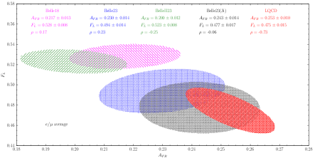
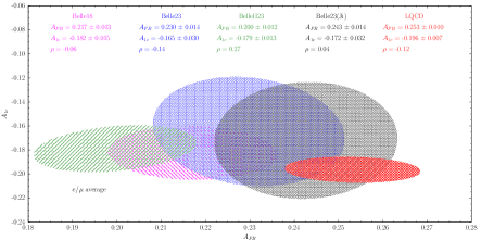
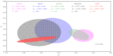
Figure 2: Contour plots (at $68\%$ probability) for the asymmetries $A_{FB}$, $F_{L}$ and $A_{1c}$ corresponding to the analyses specified in the insets and given in Table 2. In the insets the quantity $\rho$ represents the correlation coefficient.

In Ref. Belle:2023xgj the partially-integrated angular coefficients $\widehat{J}_{i}(w_{n})$ have been determined in four $w$-bins, namely

$$\widehat{J}_{i}(w_{n})\equiv\int_{w_{n-1}}^{w_{n}}dwJ_{i}(w)~{},\quad n=1,2,3,4$$ (53)

where $\{w_{n}\}=\{1.0,1.15,1.25,1.35,w_{max}^{\ell}\}$.

We may compare the experimental values of $\widehat{J}_{i}(w_{n})$ from Ref. Belle:2023xgj with the the theoretical predictions obtained from the LQCD FFs from Ref.  Martinelli:2023fwm . The differences between the theory and the experiment, which can be considered only in the case of the Belle23(Ji) data, never exceed a $2\sigma$ level. The results are presented in Fig. 3.

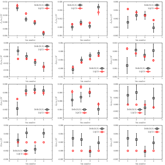
Figure 3: Normalized angular coefficients $\widehat{J}_{i}(w_{n})/{\cal{N}}$, where ${\cal{N}}$ is given in Eq. (15). The red circles represent the SM predictions corresponding to the hadronic FFs of the unitary DM approach of Ref. Martinelli:2023fwm based on all available LQCD results from Refs. FermilabLattice:2021cdg ; Harrison:2023dzh ; Aoki:2023qpa . The black squares are the experimental determinations of these quantities as measured by the Belle Collaboration in Ref. Belle:2023xgj . The quantities $\widehat{J}_{7}(w_{n}),\widehat{J}_{8}(w_{n}),\widehat{J}_{9}(w_{n})$ are exactly zero within the SM.

After replacing in Eqs. (19)-(23) the quantities $\overline{J}_{i}$ with the corresponding partially-integrated ones $\widehat{J}_{i}(w_{n})$, the five hadronic parameters $\{\eta,\eta^{\prime},\delta,\epsilon,\epsilon^{\prime}\}(w_{n})$ can be determined separately in each of the four $w$-bins of Ref. Belle:2023xgj , as well as also the bin-quantities $A_{FB}(w_{n})$, $F_{L}(w_{n})$, $A_{1c}(w_{n})$ and $A_{9c}(w_{n})$, corresponding to Eqs. (4)-(7). The experimental results for $A_{FB}(w_{n})$, $F_{L}(w_{n})$, $A_{1c}(w_{n})$ and $A_{9c}(w_{n})$ from Belle23(Ji) Belle:2023xgj are shown in Fig. 4 and turn out to be well consistent with the corresponding SM predictions corresponding to the hadronic FFs of the unitary DM approach of Ref. Martinelli:2023fwm , based on all available LQCD results from Refs. FermilabLattice:2021cdg ; Harrison:2023dzh ; Aoki:2023qpa .

The above findings seem to indicate that the w-dependence of the experimental angular coefficients $\widehat{J}_{i}(w_{n})$ from Ref. Belle:2023xgj is compatible, within $\simeq 2\sigma$, with the slope of the hadronic FFs obtained in Ref. Martinelli:2023fwm using all available LQCD determinations.

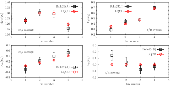
Figure 4: The bin-asymmetries $A_{FB}(w_{n})$, $F_{L}(w_{n})$, $A_{1c}(w_{n})$ and $A_{9c}(w_{n})$, evaluated separately in the four $w$-bins of Ref. Belle:2023xgj (see text) and compared with the corresponding SM predictions corresponding to the hadronic FFs of the unitary DM approach of Ref. Martinelli:2023fwm based on all available LQCD results from Refs. FermilabLattice:2021cdg ; Harrison:2023dzh ; Aoki:2023qpa .

V Conclusion

From a general, model independent analysis of the angular distributions in semileptonic $B\to D^{*}\ell\nu_{\ell}$ decays, we have shown that for $A_{FB}$, $F_{L}$ and $A_{1c}$ there are visible differences between different experimental data sets within about two standard deviations, Fig. 2. Similar differences exist between the SM predictions, based on the FFs computed in LQCD, and some sets of data. A remarkable good agreement is observed between the experimental data of Ref. Belle:2023xgj and the SM theoretical predictions, as shown in Figs. 3 and 4. In this work our approach has been applied to the case of the decay data for light leptons. It can be clearly extended to the case of final $\tau$ leptons once experimental data will be available.