Accelerating solutions of the Korteweg-de Vries equation

Abstract

The Korteweg-de Vries equation is a fundamental nonlinear equation that describes solitons with constant velocity. On the contrary, here we show that this equation also presents accelerated wavepacket solutions. This behavior is achieved by putting the Korteweg-de Vries equation in terms of the Painlevé I equation. The accelerated waveform solutions are explored numerically showing their accelerated behavior explicitly.

I Introduction

The Korteweg-de Vries (KdV) equation is widely recognized as a fundamental tool for describing nonlinear wave phenomena across various scientific disciplines whitham1974linear ; drazin1989solitons ; scott2003nonlinear ; remoissenet2013waves , with the solitary wave, or soliton, being one of its notable closed-form solutions. First derived in 1895 korteweg1895change , the KdV equation was formulated to model the propagation of surface water waves, demonstrating that the soliton represents the displacement of the water surface from its equilibrium.

Solitons are localized structures that arise in systems where nonlinearity and dispersion are delicately balanced. Due to this equilibrium, solitons are remarkably stable, maintaining their shape and velocity even after interactions with other solitons. The observation of these nonlinear waveforms in a variety of natural contexts has led to significant theoretical developments, with applications spanning fields such as optics Alhami2022 ; He2014 ; Horsley2016 , fluid dynamics BOUSSINESQ1877 ; Tian2001 , conducting polymers NARIBOLI1970661 ; Crighton1995 , gravitation suleimanov1994onset ; lidsey2012cosmology , and biology bilotta2013cellular ; carstea2015coupled , among others. For instance, in fluid dynamics, its original context, the KdV equation is used for studying ocean waves, tidal bores, and internal waves in stratified fluids. In plasma physics, is very common to use the KdV equation to describe the dynamics of ion-acoustic waves, magnetoacoustic waves and Alfvén waves in inhomogeneous plasmas, such as a dusty plasma tran1974korteweg ; tariq2023backlund ; mowafy2008effect ; zhang2023application . In nonlinear optics, the KdV equation helps the understanding of pulse propagation in optical fibers and waveguides rodriguez2003standard . These optical solitons are very important for modern telecommunications, where they help mitigate signal degradation. The KdV equation also finds applications in biological systems, particularly in the study of nerve pulse propagation fongang2018breathing .

The general form of the KdV equation is mathematically represented as

$$\frac{\partial\phi}{\partial t}+p\phi\frac{\partial\phi}{\partial\xi}+q\frac{\partial^{3}\phi}{\partial\xi^{3}}=0\ ,$$ (1)

where $\phi(t,\xi)$ is the wave profile as a function of time $t$ and a position-like coordinate $\xi$. Besides, $p$ is the nonlinear coefficient and $q$ the dispersion coefficient.

It is well-known that Eq. (1) is integrable allowing for exact solutions, including the soliton solution. These solitons have constant velocity propagation (no acceleration), as it is summarized in Sec. II. However, we show here that other propagating solutions, with not constant velocity, are possible to be found. The aim of this work is to investigate and discuss a new kind of accelerated solution of the KdV equation, which differs from the conventional soliton solution, in its form of propagation as well as its wave profile. This analytically accelerated wave solution, presented in Sec. III, is formed by a wavepacket that satisfies a Painlevé I equation, and that mainly propagates along the accelerated coordinate, depending on $t^{2}$. In Sec. IV, the behavior of this solution is numerically studied, to finish with a discussion on the implications of this solution in Sec. V.

II Soliton solution

Typically, the soliton solution of Eq. (1) has the form WAZWAZ2008485

$$\phi\left(t,\xi\right)=\phi_{0}\ \text{sech}^{2}\left(\frac{\eta}{\Delta}\right)\ ,$$ (2)

where $\eta=\xi-vt$ is the coordinate solidary to the soliton propagation, with constant $v$, representing a velocity-like quantity. Besides, $\phi_{0}=3v/p$ is the amplitude of the soliton that depends on the nonlinear coefficient $p$. Also, $\Delta=\sqrt{4|q|/v}$ represents the soliton width, depending on the dispersion coefficient $q>0$. Notice that this a travelling soliton solution, which does not exist for $v=0$.

The soliton (2) travels with constant velocity, as it can be seen by considering the coordinate frame $\eta=\mbox{constant}$, which implies $d\xi/dt=v$. This an inherent feature of solitons satisfying Eq. (1).

On the other hand, when $q<0$, the travelling soliton solution becomes fan2003new ; winkler2024existence

$$\phi\left(t,\xi\right)=\frac{\phi_{0}}{2}\text{tanh}^{2}\left(\frac{\eta}{\Delta\sqrt{2}}\right)\ ,$$ (3)

where the amplitude of the soliton is reduced in half and its width is increased by $\sqrt{2}$. This soliton also travels with constant velocity.

Both soliton solutions (2) and (3) have opposite behaviors. When the soliton (2) is compressive (rarefactive), the soliton (3) is rarefactive (compressive). However, both propagate with the same constant velocity.

III Accelerating wavepacket

Contrary to the previous section, here we show that Eq. (1) has also accelerated solutions. This means that the wave profile $\phi$ will depend on a combination of coordinates that make the velocity change, such as $d\xi/dt\neq\mbox{constant}$. As we will see below, this implies that constant accelerated propagation is only possible for a wavepacket, not for a soliton.

Let us consider the ansazt for the waveform as

$$\phi\left(t,\xi\right)=a\,\gamma\,\varphi(x)+\frac{a}{p}t\,,$$ (4)

depending on the accelerated coordinate

$$x=\alpha\left(\xi-\frac{1}{2}at^{2}\right)\,.$$ (5)

Here, $\gamma$ and $\alpha$ are constants to be determined, and $a$ can be understood as the acceleration of propagation of the wavepacket. The function $\varphi$ determines the profile of the accelerated wavepacket. Notice that the form of the ansatz has been chosen such that it identically vanishes when there is no acceleration, $a=0$.

Using the profile (4), Eq. (1) can be written for $\varphi$ in terms of coordinate $x$ as

$$\frac{\partial^{3}\varphi}{\partial x^{3}}+\lambda\frac{\partial\varphi^{2}}{\partial x}+\delta =0$$ (6)

where $\lambda=ap\gamma/(2q\alpha^{2})$, and $\delta=1/(pq\alpha^{3}\gamma)$. Both parameters quantify the relation between acceleration, the nonlinear coefficient and the dispersion coefficient.

A closer look into Eq. (6) reveals that it can be integrated to

$$\frac{\partial^{2}\varphi}{\partial x^{2}}+\lambda\varphi^{2}+\delta x =0\ ,$$ (7)

where we have set the integration constant to be $0$. From here, we notice that when $\lambda=-6$ and $\delta=-1$, then Eq. (7) turns into a Painlevé I equation

$$\frac{\partial^{2}\varphi}{\partial x^{2}}=6\varphi^{2}+x\,,$$ (8)

which is achieved under the specific choices for

$$\alpha = \left(\frac{a}{12q^{2}}\right)^{1/5}\,,$$ (9)

$$\gamma = -\frac{1}{pq}\left(\frac{a}{12q^{2}}\right)^{-3/5}\,.$$ (10)

Eq. (8) is the main result of this work. It shows that the KdV equation can be put in terms of the Painlevé I equation for a wavepacket with accelerated propagation along coordinate (5), implying that $d\xi/dt=at$. This produces a typical accelerated (parabolic) behavior in $\xi$-$t$ space.

Furthermore, the dynamics of the solution is solely determined by the constant parameters $p$, $q$, and $a$, the same number of parameter than the soliton solution ($p$, $q$, and $v$). In order to properly show the impact of the acceleration parameter $a$ on the wavepacket propagation, Eq. (8) can be solved numerically. In general, solutions of Eq. (8) do not represent a solitary wave.

IV Numerical solution

Eq. (8) is the first of six equations, where their solutions are the Painlevé transcendents davis1960introduction ; Ablowitz_Clarkson_1991 ; CLARKSON2003 . They have been highly studied in the context of dispersive long waves, pumped Maxwell-Bloch systems and physical problems leading to second order ordinary differential equations porsezian1995optical ; feng2017nonlocal ; levi2013painleve

In order to evaluate the accelerated solution (4), we solve numerically Eq. (8). This is shown in Figs. 1 and 2, in terms of density plots. To find this solution, we set values for the nonlinear coefficient $p$, the dispersion coefficient $q$ and the acceleration-like parameter $a$, that make the solution a real function. To solve Eq. (8), we chose the initial conditions $\varphi(x=0)=0.1$ and $d_{x}\varphi(x=0)=0$. In general, we see that each part of the wavepacket follows accelerated (parabolic) trajectories, represented by the dashed lines on both figures. These curves are determined by the constant value of the accelerated coordinate (5) (defining different initial conditions). Therefore, all the curved trajectories satisfy $d^{2}\xi/dt^{2}=a$. In both figures, for the curves, we have chose different initial positions at $x=-2,-4,-6,-8,-10,-12$.

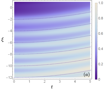
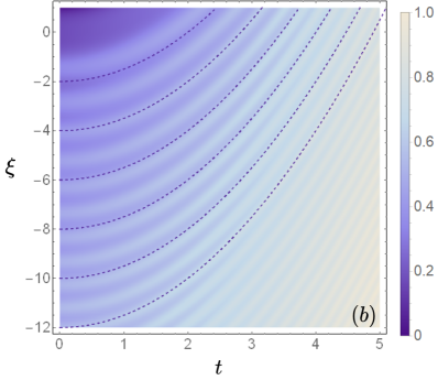
Figure 1: Density plot for solution $\phi(t,\xi)$ [Eq. (4)], with $p=20$ and $q=0.1$, and initial conditions $\varphi(x=0)=0.1$ and $d_{x}\varphi(x=0)=0$. Dashed lines represent parabolic trajectories for (a) $a=0.1$, and (b) $a=1$.

In Fig. 1 we explore two different values for the acceleration parameter $a$. The parabolic behaviour of the wave train (4) is altered by the value of this parameter, increasing the curvature of the trajectory for higher values of $a$. In Fig. 1(a) we show the accelerated solution (4) for $a=0.1$. In this case, the wavepacket has several minima and maxima, all following the accelerated coordinate (5). In Fig. 1(b) we change the value of acceleration to $a=1$, where the increase in the curvature of the trajectory that the wave follows can be easily seen for the same initial conditions. The increase on curvature of the trajectories is a direct consequence of the larger acceleration of the wavepacket. In both cases we use fixed values for the $p$ and $q$ coefficients, demonstrating the sole effect of acceleration.

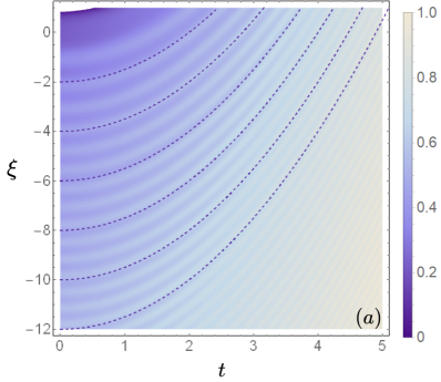
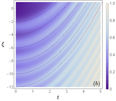
Figure 2: Density plot for $\phi(t,\xi)$ [Eq. (4)], with $p=20$ and $a=1$, for initial conditions $\varphi(x=0)=0.1$ and $d_{x}\varphi(x=0)=0$. Dashed lines represent parabolic trajectories for (a) $q=0.05$ and (b) $q=0.5$.

According to Eqs. (9) and (10), the nonlinear and dispersion coefficients are free parameters that modified the characteristics of the wave train, for a given acceleration. This is depicted in Fig. 2. When the parameter $q$ is allowed to change, we can observe how dispersion changes for the accelerated solution. For low values of $q$, the wavepacket has more minima and maxima than in the case shown in Fig. 1, and they seem to appear less often than with higher values of $q$. This is the expected behavior of dispersion. This can be seen in Figs. 2(a) and 2(b), where we have used $q=0.05$ and $q=0.5$, respectively. In both cases is shown by dashed lines that modifying the dispersion coefficient does not change the trajectory of the wave packet. This is because the accelerated coordinate (5) does not depend on $q$. Thus, for different values of $q$, the parabolic trajectories remain unchanged for different initial conditions.

V Summary

In this study we demonstrate that the Korteweg-de Vries equation (1) also have a set of accelerating wavepacket solutions, distinct from solitons. This result expands the understanding of nonlinear wave dynamics to a new class of unexplored solutions.

This accelerated wave train is obtained by reducing the KdV equation into a Painlevé I equation, in terms of an accelerated coordinate system. Thus, the new solution for the KdV equation describes a wavepacket following a parabolic trajectory in $\xi$-$t$ space, and it is susceptible to changes due to the different parameters, specifically the acceleration $a$ and the dispersion coefficient $q$.

This solution for the KdV equation belongs to a new class of accelerated solutions for nonlinear dynamics systems, such as the ones described by the nonlinear Schrödinger equation Asenjonon . Thus, we think that the presented results contribute to a novel understanding on the KdV equation’s versatility, and its relevance in modern theoretical and applied physics.

References

- (1) G. Whitham, Linear and Nonlinear Waves (Wiley, 1974).
- (2) P. Drazin and R. Johnson, Solitons: An Introduction (Cambridge University Press, 1989).
- (3) A. Scott, Nonlinear Science: Emergence and Dynamics of Coherent Structures, 2nd ed. (Oxford University Press, 2003).
- (4) M. Remoissenet, Waves Called Solitons: Concepts and Experiments (Springer Science & Business Media, 2013).
- (5) D. Korteweg and G. de Vries, Phyl. Mag. 39, 422 (1895).
- (6) R. Alhami and M. Alquran, Opt. Quantum Electron. 54, 553 (2022).
- (7) J. He, L. Wang, L. Li, K. Porsezian, and R. Erdélyi, Phys. Rev. E 89, 062917 (2014).
- (8) S. A. R. Horsley, J. Opt. 18, 085104 (2016).
- (9) J. Boussinesq, Bibliothèque nationale de France 1 vol. (XXII-680-61 p.), 680 (1877).
- (10) B. Tian and Y.-T. Gao, Eur. Phys. J. B 22, 351 (2001).
- (11) G. Nariboli and A. Sedov, J. Math. Anal. Appl. 32, 661 (1970).
- (12) D. G. Crighton, Acta Appl. Math. 39, 39 (1995).
- (13) B. Suleimanov, Zhurn. Eskper. Teor. Fiz 105, 1089 (1994).
- (14) J. E. Lidsey, Phys. Rev. D 86, 123523 (2012).
- (15) E. Bilotta and P. Pantano, Int. J. Bifurcat. Chaos 23, 1330003 (2013).
- (16) A. Carstea and T. Tokihiro, J. Phys. A 48, 055205 (2015).
- (17) M. Q. Tran and P. J. Hirt, Plasma Physics 16, 617 (1974).
- (18) M. S. Tariq et al., Phys. Fluids 35 (2023).
- (19) A. Mowafy, E. El-Shewy, W. Moslem, and M. Zahran, Phys. Plasmas 15 (2008).
- (20) H. Zhang et al., J. Plasma Phys. 89, 905890212 (2023).
- (21) R. Rodríguez, J. Reyes, A. Espinosa-Cerón, J. Fujioka, and B. Malomed, Phys. Rev. E 68, 036606 (2003).
- (22) G. Fongang Achu, F. Moukam Kakmeni, and A. Dikande, Phys. Rev. E 97, 012211 (2018).
- (23) A.-M. Wazwaz, Chapter 9 the kdv equation, , Handbook of Differential Equations: Evolutionary Equations Vol. 4, pp. 485–568, North-Holland, 2008.
- (24) E. Fan, Chaos, Solitons & Fractals 15, 567 (2003).
- (25) M. A. Winkler, V. Muñoz, and F. A. Asenjo, Fundamental Plasma Physics 9, 100030 (2024).
- (26) H. Davis and U. A. E. Commission, Introduction to Nonlinear Differential and Integral Equations (U.S. Atomic Energy Commission, 1960).
- (27) M. A. Ablowitz and P. A. Clarkson, Solitons, Nonlinear Evolution Equations and Inverse ScatteringLondon Mathematical Society Lecture Note Series (Cambridge University Press, 1991).
- (28) P. A. Clarkson, J. Comput. Appl. Math. 153, 127 (2003), Proceedings of the 6th International Symposium on Orthogonal Poly nomials, Special Functions and their Applications, Rome, Italy, 18-22 June 2001.
- (29) K. Porsezian and K. Nakkeeran, J. Mod. Opt. 42, 1953 (1995).
- (30) L.-L. Feng, S.-F. Tian, and T.-T. Zhang, Z. Naturforsch 72, 425 (2017).
- (31) D. Levi and P. WinternitzPainlevé transcendents: their asymptotics and physical applications Vol. 278 (Springer Science & Business Media, 2013).
- (32) F. A. Asenjo, J. Plasma Phys. 90, 905900119 (2024).