Initial data for a deformed isolated horizon

Abstract

Within the isolated horizon formalism, we investigate a static axisymmetric space-time of a black hole influenced by matter in its neighborhood. To illustrate the role of ingredients and assumptions in this formalism, we first show how, in spherical symmetry, the field equations and gauge conditions imply the isolated horizon initial data leading to the Schwarzschild space-time. Then, we construct the initial data for a static axisymmetric isolated horizon representing a deformed black hole. The space-time description in the Bondi-like coordinates is then found as a series expansion in the vicinity of the horizon. To graphically illustrate this construction, we also find a numerical solution for a black hole deformed by a particular analytic model of a thin accretion disk. We also discuss how an accretion disk affects the analytical properties of the horizon geometry.

I Introduction

The isolated horizon (IH) formalism [1] has proven to be a powerful framework for the description of black holes in equilibrium. These black holes can have arbitrary time-independent intrinsic geometry, the space-time does not have to be asymptotically flat, and outside the horizon it may be dynamical due to outgoing gravitational and electromagnetic radiation. One of the key features of the isolated horizon formalism is the applicability of the standard laws of black hole thermodynamics [2]. Another important characteristic is the quasi-locality of the description. Thanks to it, unlike event horizons, isolated horizons do not require knowledge of the entire space-time and avoid having central quantities defined both at infinity (angular momentum, mass) and at the horizon (surface gravity, angular velocity). This quasi-locality was essential in the computation of entropy in quantum gravity [3]. The more general scenario, where in-falling matter is present, has also been explored within the more universal framework of dynamical horizons, [4, 5].

Both the mechanics of isolated horizons, [6, 7, 2, 8, 9], and their intrinsic geometry, [10, 11, 12, 13], have been extensively studied. In [14], general solutions of the Einstein field equations admitting isolated horizons were studied. Interestingly, while the intrinsic geometry can coincide with the Kerr–Newman black hole, the neighborhood can be distorted. The geometry around an isolated horizon has been investigated in [15], where the isolated horizon was specified as the characteristic initial value formulation. A general review of such a formulation can be found in [16]. For more information, see the references in [15]. However, the construction in [15] did not provide any clues on how to choose the initial data. This issue was partially addressed in [17], where the Kinnersley tetrad was transformed to obtain the initial data for Kerr space-time. Nevertheless, the obtained tetrad was not in an explicit form. This has been recently revised in [18].

Moreover, while the Kerr example is physically interesting, the solution of [17] was only obtained thanks to the prior knowledge of the solution and its properties. Hence, we shall start by following the construction of a tetrad describing an isolated horizon as shown by [15] (performed using the Newman–Penrose (NP) formalism [19]) and finding the initial data for spherical symmetry in the isolated horizon formalism. Although this is a simpler (and astrophysically less important) example, no prior knowledge of the resulting metric is used, the properties of the isolated horizons are demonstrated in action, and the result shall serve as a starting point for the next section.

Isolated horizons are also suitable for describing models of astrophysical black holes, as they can describe deformations of the horizon geometry caused by static distribution of matter without compromising the horizon isolation. The metric of a black hole and surrounding matter have been studied, e.g. in [20, 21] for the Schwarzschild and Kerr black holes. In this paper, we investigate a Schwarzschild black hole deformed by the presence of matter in its neighborhood (such as an “accretion” disk) in the isolated horizon formalism using the Weyl superimposed metric from [22]. A disk derived in [23] is later used as a particular example. We shall see that, while the Weyl coordinates are usually easier to use due to their simplicity, since they are singular at the horizon, they are not always well suited. The coordinate transformation to Bondi-like coordinates is not obvious. Our work might thus be useful whenever checking the on-horizon limit of a certain process is required or desirable. Importantly, the results are not based on the perturbation approach; the Weyl metric allows to consider strong-field deformations of the black hole horizon. Very recently, first-order tidal deformations of isolated horizons were studied in [24].

In the next section, we briefly introduce the isolated horizons and the coordinates and tetrad of [15]. We review the initial value problem and an axial isolated horizon as introduced by Ashtekar. Then, in Sec. III, we discuss spherical symmetry in the isolated horizon formalism and construct the initial data and tetrad describing it. This is then used in Sec. IV as a starting point for deformation of a non-rotating black hole in the isolated horizon formalism. The set of initial data for isolated horizons is large and not thoroughly studied. We select the subspace corresponding to an arbitrarily strong deformation of the Schwarzschild black hole horizon and construct both initial data and the near-horizon series expansion of the solution in Bondi-like coordinates. While the deformation is considered analytically (as a series) and generally, it is complemented in Sec. V with one particular example produced numerically. Finally, in Sec. VI, we discuss some important properties such as the convergence of the solution. The description of the numerical solution, its precision, and comparison are, together with the review of the NP formalism and the particular solution of the disk, postponed to the appendices.

A geometrized unit system is used, where $c=1$ and $G=1$. Moreover, the space-time metric $g_{ab}$ has the signature $({+}{-}{-}{-})$ and the Riemann tensor is defined by $2\nabla_{[c}\nabla_{d]}\,X^{a}=-R^{a}{}_{bcd}X^{b}$.

II Isolated horizons, coordinates and tetrad

A Bondi-like coordinate system and adapted Newman–Penrose null tetrad for weakly isolated horizons have been introduced in [15] and the details of the construction were spelled out in detail in [25]. Here we do not repeat the construction and only review the results. For a brief review of the Newman–Penrose formalism, see Appendix A. The coordinates will be denoted by ${\color[rgb]{1,0,0}{\mathsfit{x}}}^{\mu}=({\color[rgb]{1,0,0}{u}},{\color[rgb]{1,0,0}{s}},{\color[rgb]{1,0,0}{\vartheta}},{\color[rgb]{1,0,0}{\varphi}})$, $\mu=0,1,2,3$ where, on the horizon $\mathcal{H}$, ${\color[rgb]{1,0,0}{u}}$ is the parameter along the null generators of $\mathcal{H}$ and the submanifolds ${\color[rgb]{1,0,0}{u}}=\mathrm{constant}$ are null hypersurfaces intersecting $\mathcal{H}$ (given by ${\color[rgb]{1,0,0}{s}}=0$) at topological 2-spheres with coordinates ${\color[rgb]{1,0,0}{\mathsfit{x}}}^{I}$, $I=2,3$. In particular, the sphere given by ${\color[rgb]{1,0,0}{s}}=0,{\color[rgb]{1,0,0}{u}}=0$ will be denoted by $\SS_{0}$.

Appropriate NP tetrad $e_{\mu}{}^{a}$ adapted to these coordinates consists of four null vectors named ${\color[rgb]{0,0,1}{\ell\kern 0.20004pt}}^{a}$, ${\color[rgb]{0,0,1}{n}}^{a}$ and ${\color[rgb]{0,0,1}{m}}^{a}$ and its complex conjugate $\mkern 2.0mu\overline{\mkern-2.0mu{\color[rgb]{0,0,1}{m}}\mkern-0.7mu}\mkern 0.7mu^{a}$. Their coordinate expressions read as follows:

$$\begin{aligned} \boldsymbol{{\color[rgb]{0,0,1}{\ell\kern 0.20004pt}}}&=\partial_{\color[rgb]{1,0,0}{u}}+U\,\partial_{\color[rgb]{1,0,0}{s}}+X^{I}\,\partial_{I}\,,\\ \boldsymbol{{\color[rgb]{0,0,1}{n}}}&=-\,\partial_{\color[rgb]{1,0,0}{s}}\,,\\ \boldsymbol{{\color[rgb]{0,0,1}{m}}}&=\mathit{\Omega}\,\partial_{\color[rgb]{1,0,0}{s}}+\xi^{I}\,\partial_{I}\,.\end{aligned}$$ (1)

Since the NP projections of the fields and the spin coefficients depend on the geometry itself as well as on the tetrad, we understand all tetrad projections with respect to this geometrically motivated tetrad.

Following the standard NP notation, [19], we introduce the directional derivatives associated with the respective null vectors as

$${\color[rgb]{0,0,1}{\mathrm{D}}} \equiv{\color[rgb]{0,0,1}{\ell\kern 0.20004pt}}^{a}\nabla_{a}\,, {\color[rgb]{0,0,1}{\Delta}} \equiv{\color[rgb]{0,0,1}{n}}^{a}\nabla_{a}\,, {\color[rgb]{0,0,1}{\updelta}} \equiv{\color[rgb]{0,0,1}{m}}^{a}\nabla_{a}\,.$$

The coefficients appearing in the expressions of the vectors will be referred to as the metric functions. Functions $U,X^{I}$ and $\mathit{\Omega}$ vanish on the horizon, i.e.

$$U\mathbin{\dot{=}}X^{I}\mathbin{\dot{=}}\mathit{\Omega}\mathbin{\dot{=}}0\,,$$

where we use symbol $\mathbin{\dot{=}}$ for the equality of two quantities on the horizon $\mathcal{H}$ but not necessarily elsewhere. Hence, $\boldsymbol{{\color[rgb]{0,0,1}{\ell\kern 0.20004pt}}}\mathbin{\dot{=}}\partial_{\color[rgb]{1,0,0}{u}}$ is tangent to the null geodesics generating $\mathcal{H}$ but, in general, it is not affinely parameterized, its acceleration being the surface gravity $\kappa_{({\color[rgb]{0,0,1}{\ell\kern 0.14003pt}})}$ defined by

$${\color[rgb]{0,0,1}{\mathrm{D}}}{\color[rgb]{0,0,1}{\ell\kern 0.20004pt}}^{a} \mathbin{\dot{=}}\kappa_{({\color[rgb]{0,0,1}{\ell\kern 0.14003pt}})}\,{\color[rgb]{0,0,1}{\ell\kern 0.20004pt}}^{a}\,.$$

On the horizon, vectors ${\color[rgb]{0,0,1}{m}}^{a}$ and $\mkern 2.0mu\overline{\mkern-2.0mu{\color[rgb]{0,0,1}{m}}\mkern-0.7mu}\mkern 0.7mu^{a}$ span the tangent space to the 2-spheres ${\color[rgb]{1,0,0}{s}}=0$, ${\color[rgb]{1,0,0}{u}}=\mathrm{constant}$. We can choose these vectors (or equivalently functions $\xi^{I}$) arbitrarily on $\SS_{0}$ and propagate them along $\mathcal{H}$ using the Lie derivative $\mathcal{L}$ by demanding

$$\mathcal{L}_{\boldsymbol{{\color[rgb]{0,0,1}{\ell\kern 0.14003pt}}}}{\color[rgb]{0,0,1}{m}}^{a} \mathbin{\dot{=}}0\,.$$

The choice of ${\color[rgb]{0,0,1}{\ell\kern 0.20004pt}}^{a}$ and ${\color[rgb]{0,0,1}{m}}^{a}$ on $\mathcal{H}$ uniquely determines vector ${\color[rgb]{0,0,1}{n}}^{a}$. Finally, we propagate the tetrad from the horizon to its neighborhood by conditions

$${\color[rgb]{0,0,1}{\Delta}}{\color[rgb]{0,0,1}{\ell\kern 0.20004pt}}^{a}={\color[rgb]{0,0,1}{\Delta}}{\color[rgb]{0,0,1}{n}}^{a}={\color[rgb]{0,0,1}{\Delta}}{\color[rgb]{0,0,1}{m}}^{a}=0\,.$$ (2)

Moreover, we require $\mathcal{H}$ to be a non-expanding horizon. That is, $\mathcal{H}$ is a null hypersurface with vanishing expansion, the Einstein field equations and an energy condition are satisfied on the horizon. The non-expanding horizon is then paired with a (class of) null normal(s) ${\color[rgb]{0,0,1}{\ell\kern 0.20004pt}}^{a}$ to create either a weakly isolated horizon or (strongly) isolated horizon in the sense of [10]. For a weakly isolated horizon, the intrinsic geometry has to satisfy:

$$[\mathcal{L}_{\boldsymbol{{\color[rgb]{0,0,1}{\ell\kern 0.14003pt}}}},\mathcal{D}_{a}]{\color[rgb]{0,0,1}{\ell\kern 0.20004pt}}^{b}\mathbin{\dot{=}}0\,,$$ (3)

where the covariant derivative $\mathcal{D}_{a}$ intrinsic to the horizon is defined by $Y^{a}\mathcal{D}_{a}X^{b}\mathbin{\dot{=}}Y^{a}\nabla_{a}X^{b}$ for any $X^{a}$ and $Y^{a}$ tangent to $\mathcal{H}$. Any non-expanding can be made into a weakly isolated horizon and condition (3) already makes the surface gravity $\kappa_{({\color[rgb]{0,0,1}{\ell\kern 0.14003pt}})}$ constant across the horizon ($0^{\text{th}}$ law of thermodynamics).

The stronger condition for an isolated horizon is:

$$[\mathcal{L}_{\boldsymbol{{\color[rgb]{0,0,1}{\ell\kern 0.14003pt}}}},\mathcal{D}_{a}]X^{b}\mathbin{\dot{=}}0\,,$$ (4)

for an arbitrary vector $X^{b}$ tangent to $\mathcal{H}$. This astrophysically more relevant choice is in fact a restriction on the geometry of the space-time (in contrast with the weakly isolated horizons) and makes all geometrical quantities time-independent (${\color[rgb]{1,0,0}{u}}$-independent) on $\mathcal{H}$. It can be shown that Eq. (4) is equivalent to ${\color[rgb]{0,0,1}{\ell\kern 0.20004pt}}^{a}$ satisfying the Killing equations up to the second order in ${\color[rgb]{1,0,0}{s}}$.

Conditions imposed on the tetrad enumerated above translate into the properties of the NP spin coefficients as follows:

$$\begin{aligned} {\color[rgb]{0,0,1}{\mu}}&=\mkern 2.0mu\overline{\mkern-2.0mu{\color[rgb]{0,0,1}{\mu}}\mkern-0.7mu}\mkern 0.7mu\,,\\ {\color[rgb]{0,0,1}{\tau}}&={\color[rgb]{0,0,1}{\gamma}}={\color[rgb]{0,0,1}{\nu}}=0\,,\\ {\color[rgb]{0,0,1}{\pi}}&={\color[rgb]{0,0,1}{\alpha}}+\mkern 2.0mu\overline{\mkern-2.0mu{\color[rgb]{0,0,1}{\beta}}\mkern-0.7mu}\mkern 0.7mu\,,\\ {\color[rgb]{0,0,1}{\varepsilon}}&\mathbin{\dot{=}}\mkern 2.0mu\overline{\mkern-2.0mu{\color[rgb]{0,0,1}{\varepsilon}}\mkern-0.7mu}\mkern 0.7mu=\frac{\kappa_{({\color[rgb]{0,0,1}{\ell\kern 0.14003pt}})}}{2}\,,\quad\kappa_{({\color[rgb]{0,0,1}{\ell\kern 0.14003pt}})}\mathbin{\dot{=}}\mathrm{constant}\,,\\ {\color[rgb]{0,0,1}{\rho}}&\mathbin{\dot{=}}{\color[rgb]{0,0,1}{\sigma}}\mathbin{\dot{=}}{\color[rgb]{0,0,1}{\kappa}}\mathbin{\dot{=}}0\,.\end{aligned}$$ (5)

The fact that ${\color[rgb]{0,0,1}{\mu}}$ is real implies that congruence ${\color[rgb]{0,0,1}{n}}^{a}$ is twist-free; vanishing of spin coefficients ${\color[rgb]{0,0,1}{\rho}},{\color[rgb]{0,0,1}{\sigma}}$ and ${\color[rgb]{0,0,1}{\kappa}}$ on the horizon expresses the fact that $\mathcal{H}$ is both non-expanding, non-twisting and shear-free and ${\color[rgb]{0,0,1}{\ell\kern 0.20004pt}}^{a}$ is geodesic. It is also convenient to introduce quantity

$$\begin{aligned} {\color[rgb]{0,0,1}{a}}&={\color[rgb]{0,0,1}{\alpha}}-\mkern 2.0mu\overline{\mkern-2.0mu{\color[rgb]{0,0,1}{\beta}}\mkern-0.7mu}\mkern 0.7mu={\color[rgb]{0,0,1}{m}}^{a}\,\mkern 2.0mu\overline{\mkern-2.0mu{\color[rgb]{0,0,1}{\updelta}}\mkern-0.7mu}\mkern 0.7mu\mkern 2.0mu\overline{\mkern-2.0mu{\color[rgb]{0,0,1}{m}}\mkern-0.7mu}\mkern 0.7mu_{a}\,.\end{aligned}$$

On the horizon, it encodes the induced 2-dimensional connection on $\SS_{0}$.

II.1 Initial value problem

Space-time near an isolated horizon can be reconstructed as the solution of characteristic initial value problem with the initial data given on $\mathcal{H}$ itself and another null hypersurface intersecting $\mathcal{H}$, [15]. In the Bondi-like coordinates introduced in Sec. II, such hypersurfaces $\mathcal{N}_{\color[rgb]{1,0,0}{u}}$ are conveniently represented by equation ${\color[rgb]{1,0,0}{u}}=\mathrm{constant}$. Then the 2-spheres foliating the horizon are simply $\SS_{\color[rgb]{1,0,0}{u}}=\mathcal{H}\cap\mathcal{N}_{\color[rgb]{1,0,0}{u}}$. In our setting, we will formulate the initial value problem on $\mathcal{H}$ and $\mathcal{N}_{0}$ which intersect at $\SS_{0}$.

As discussed in [15], the free initial data consist of the following quantities.

• Free data on $\SS_{0}$:

  • constant surface gravity $\kappa_{({\color[rgb]{0,0,1}{\ell\kern 0.14003pt}})}={\color[rgb]{0,0,1}{\varepsilon}}+\mkern 2.0mu\overline{\mkern-2.0mu{\color[rgb]{0,0,1}{\varepsilon}}\mkern-0.7mu}\mkern 0.7mu$,

  • spin coefficients ${\color[rgb]{0,0,1}{\pi}},{\color[rgb]{0,0,1}{a}},{\color[rgb]{0,0,1}{\lambda}},{\color[rgb]{0,0,1}{\mu}}$,

  • metric functions $\xi^{I}$,

• Free data on $\mathcal{N}_{0}$:

  • Weyl component ${\color[rgb]{0,0,1}{\kern-1.00006pt\mathit{\Psi}\kern-0.80002pt}}_{4}$;

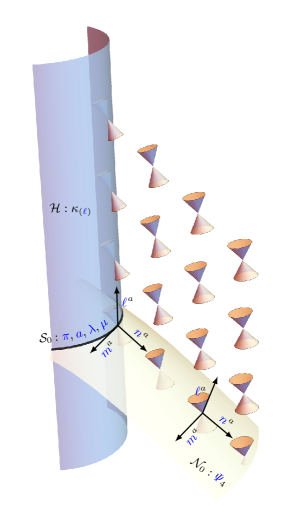
Figure 1: The neighborhood of the horizon and initial value surfaces. The scalars enlisted after the colons have to be introduced on the corresponding hypersurface. Moreover, we need to know the complete tetrad on the horizon.

The situation is schematically visualized in Fig. 1.

Properties of a vacuum weakly isolated horizon enforce relations (5) and, in addition,

$${\color[rgb]{0,0,1}{\kern-1.00006pt\mathit{\Psi}\kern-0.80002pt}}_{0}\mathbin{\dot{=}}{\color[rgb]{0,0,1}{\kern-1.00006pt\mathit{\Psi}\kern-0.80002pt}}_{1}\mathbin{\dot{=}}0\,.$$

Data on $\SS_{0}$ can be propagated along the entire horizon as follows. The Weyl scalar ${\color[rgb]{0,0,1}{\kern-1.00006pt\mathit{\Psi}\kern-0.80002pt}}_{3}$ on $\mathcal{H}$ can be computed from the Ricci identity (108r) and scalar ${\color[rgb]{0,0,1}{\kern-1.00006pt\mathit{\Psi}\kern-0.80002pt}}_{4}$ is propagated via Bianchi identity (109d). On $\SS_{0}$, one can use ${\color[rgb]{0,0,1}{a}}$ and ${\color[rgb]{0,0,1}{\pi}}$ to calculate the Weyl scalar ${\color[rgb]{0,0,1}{\kern-1.00006pt\mathit{\Psi}\kern-0.80002pt}}_{2}$ by taking the real and imaginary parts of the Ricci identity (108q),

$$\operatorname{Re}\!{\color[rgb]{0,0,1}{\kern-1.00006pt\mathit{\Psi}\kern-0.80002pt}}_{2} \mathbin{\dot{=}}{\color[rgb]{0,0,1}{a}}\mkern 2.0mu\overline{\mkern-2.0mu{\color[rgb]{0,0,1}{a}}\mkern-0.7mu}\mkern 0.7mu-\frac{1}{2}\left({\color[rgb]{0,0,1}{\updelta}}{\color[rgb]{0,0,1}{a}}+\mkern 2.0mu\overline{\mkern-2.0mu{\color[rgb]{0,0,1}{\updelta}}\mkern-0.7mu}\mkern 0.7mu\mkern 2.0mu\overline{\mkern-2.0mu{\color[rgb]{0,0,1}{a}}\mkern-0.7mu}\mkern 0.7mu\right),$$

$$\operatorname{Im}\!{\color[rgb]{0,0,1}{\kern-1.00006pt\mathit{\Psi}\kern-0.80002pt}}_{2} \mathbin{\dot{=}}-\operatorname{Im}\left({\color[rgb]{0,0,1}{\updelta}}{\color[rgb]{0,0,1}{\pi}}-{\color[rgb]{0,0,1}{a}}{\color[rgb]{0,0,1}{\pi}}\right),$$

Bianchi identity (109b) shows that ${\color[rgb]{0,0,1}{\kern-1.00006pt\mathit{\Psi}\kern-0.80002pt}}_{2}$ is ${\color[rgb]{1,0,0}{u}}$-independent on $\mathcal{H}$,

$${\color[rgb]{0,0,1}{\mathrm{D}}}{\color[rgb]{0,0,1}{\kern-1.00006pt\mathit{\Psi}\kern-0.80002pt}}_{2} \mathbin{\dot{=}}0\,.$$

Ricci identities (108d) and (108e) imply

$${\color[rgb]{0,0,1}{\mathrm{D}}}{\color[rgb]{0,0,1}{\pi}} \mathbin{\dot{=}}{\color[rgb]{0,0,1}{\mathrm{D}}}{\color[rgb]{0,0,1}{a}}\mathbin{\dot{=}}0\,,$$

while the evolution of ${\color[rgb]{0,0,1}{\lambda}}$ and ${\color[rgb]{0,0,1}{\mu}}$ along $\mathcal{H}$ is given by Ricci identities (108g) and (108h):

$$\begin{aligned} {\color[rgb]{0,0,1}{\mathrm{D}}}{\color[rgb]{0,0,1}{\lambda}}&\mathbin{\dot{=}}\mkern 2.0mu\overline{\mkern-2.0mu{\color[rgb]{0,0,1}{\updelta}}\mkern-0.7mu}\mkern 0.7mu{\color[rgb]{0,0,1}{\pi}}-\mkern 2.0mu\overline{\mkern-2.0mu{\color[rgb]{0,0,1}{a}}\mkern-0.7mu}\mkern 0.7mu{\color[rgb]{0,0,1}{\pi}}+{\color[rgb]{0,0,1}{\pi}}^{2}-\kappa_{({\color[rgb]{0,0,1}{\ell\kern 0.14003pt}})}\,{\color[rgb]{0,0,1}{\lambda}}\,,\\ {\color[rgb]{0,0,1}{\mathrm{D}}}{\color[rgb]{0,0,1}{\mu}}&\mathbin{\dot{=}}{\color[rgb]{0,0,1}{\updelta}}{\color[rgb]{0,0,1}{\pi}}-{\color[rgb]{0,0,1}{a}}{\color[rgb]{0,0,1}{\pi}}+|{\color[rgb]{0,0,1}{\pi}}|^{2}+{\color[rgb]{0,0,1}{\kern-1.00006pt\mathit{\Psi}\kern-0.80002pt}}_{2}-\kappa_{({\color[rgb]{0,0,1}{\ell\kern 0.14003pt}})}\,{\color[rgb]{0,0,1}{\mu}}\,.\end{aligned}$$ (6)

Hence, the geometry of $\mathcal{H}$ is fully determined by the initial data on $\SS_{0}$. What remains is to specify scalar ${\color[rgb]{0,0,1}{\kern-1.00006pt\mathit{\Psi}\kern-0.80002pt}}_{4}$ on $\mathcal{N}_{0}$ which is free, unconstrained function of ${\color[rgb]{1,0,0}{s}},{\color[rgb]{1,0,0}{\vartheta}},{\color[rgb]{1,0,0}{\varphi}}$. Notice that for weakly isolated horizons, the NP scalars ${\color[rgb]{0,0,1}{\mu}},{\color[rgb]{0,0,1}{\lambda}},{\color[rgb]{0,0,1}{\kern-1.00006pt\mathit{\Psi}\kern-0.80002pt}}_{3}$ and ${\color[rgb]{0,0,1}{\kern-1.00006pt\mathit{\Psi}\kern-0.80002pt}}_{4}$ in general depend on time ${\color[rgb]{1,0,0}{u}}$.

After a short discussion of weakly isolated horizons in Sec. III, we will focus on isolated horizons (rather than weakly isolated ones) with axial symmetry, which imposes additional constraints. Consequently, all NP scalars are independent of coordinates ${\color[rgb]{1,0,0}{u}}$ and ${\color[rgb]{1,0,0}{\varphi}}$, in particular

$${\color[rgb]{0,0,1}{\mathrm{D}}}{\color[rgb]{0,0,1}{\mu}} \mathbin{\dot{=}}{\color[rgb]{0,0,1}{\mathrm{D}}}{\color[rgb]{0,0,1}{\lambda}}\mathbin{\dot{=}}{\color[rgb]{0,0,1}{\mathrm{D}}}{\color[rgb]{0,0,1}{\kern-1.00006pt\mathit{\Psi}\kern-0.80002pt}}_{3}\mathbin{\dot{=}}{\color[rgb]{0,0,1}{\mathrm{D}}}{\color[rgb]{0,0,1}{\kern-1.00006pt\mathit{\Psi}\kern-0.80002pt}}_{4}\mathbin{\dot{=}}0\,.$$ (7)

Therefore, Eqs. (6) simplify to

$$\begin{aligned} \mkern 2.0mu\overline{\mkern-2.0mu{\color[rgb]{0,0,1}{\updelta}}\mkern-0.7mu}\mkern 0.7mu{\color[rgb]{0,0,1}{\pi}}-\mkern 2.0mu\overline{\mkern-2.0mu{\color[rgb]{0,0,1}{a}}\mkern-0.7mu}\mkern 0.7mu{\color[rgb]{0,0,1}{\pi}}+{\color[rgb]{0,0,1}{\pi}}^{2}&\mathbin{\dot{=}}\kappa_{({\color[rgb]{0,0,1}{\ell\kern 0.14003pt}})}\,{\color[rgb]{0,0,1}{\lambda}}\,,\\ {\color[rgb]{0,0,1}{\updelta}}{\color[rgb]{0,0,1}{\pi}}-{\color[rgb]{0,0,1}{a}}{\color[rgb]{0,0,1}{\pi}}+|{\color[rgb]{0,0,1}{\pi}}|^{2}+{\color[rgb]{0,0,1}{\kern-1.00006pt\mathit{\Psi}\kern-0.80002pt}}_{2}&\mathbin{\dot{=}}\kappa_{({\color[rgb]{0,0,1}{\ell\kern 0.14003pt}})}\,{\color[rgb]{0,0,1}{\mu}}\,,\end{aligned}$$

and they further constrain ${\color[rgb]{0,0,1}{\pi}}$ and ${\color[rgb]{0,0,1}{\kern-1.00006pt\mathit{\Psi}\kern-0.80002pt}}_{2}$ provided that ${\color[rgb]{0,0,1}{\lambda}}$ and ${\color[rgb]{0,0,1}{\mu}}$ are free functions on $\SS_{0}$.

II.2 Axial symmetry

Let us now introduce an axially symmetric (weakly) isolated horizon as defined in [26].

Definition 1 (Axially symmetric isolated horizon).

An isolated horizon is axially symmetric if any 2-sphere $\mathcal{S}_{\color[rgb]{1,0,0}{u}}$, defined by ${\color[rgb]{1,0,0}{s}}=0$, ${\color[rgb]{1,0,0}{u}}=\mathrm{constant}$, possesses a space-like Killing vector with closed orbits whose norm vanishes exactly at two points called the north and south poles.

Note that the axial symmetry is only defined for the isolated horizon itself, not the space-time admitting the horizon. Then, as shown in [26], one can introduce the coordinates ${\color[rgb]{1,0,0}{\mathsfit{x}}}^{I}=({\color[rgb]{1,0,0}{\varsigma}},{\color[rgb]{1,0,0}{\varphi}})$ with ${\color[rgb]{1,0,0}{\varsigma}}\in[-1,1]$ and ${\color[rgb]{1,0,0}{\varphi}}\in[0,2\kern 0.39993pt\uppi\kern 0.39993pt)$. In this coordinates the metric on $\mathcal{S}_{\color[rgb]{1,0,0}{u}}$ is of the form

$$\boldsymbol{q}=-{\color[rgb]{0.5,0.5,0}{\mathcal{R}}}^{2}\left(h({\color[rgb]{1,0,0}{\varsigma}})^{-1}\,\mathrm{d}{\color[rgb]{1,0,0}{\varsigma}}^{2}+h({\color[rgb]{1,0,0}{\varsigma}})\,\mathrm{d}{\color[rgb]{1,0,0}{\varphi}}^{2}\right).$$ (8)

Here, ${\color[rgb]{0.5,0.5,0}{\mathcal{R}}}$ is the Euclidean radius defined by $A=4\kern 0.39993pt\uppi\kern 0.39993pt{\color[rgb]{0.5,0.5,0}{\mathcal{R}}}^{2}$ and $A$ is the geometrically defined area of the 2-sphere $\mathcal{S}_{\color[rgb]{1,0,0}{u}}$. The positive function $h({\color[rgb]{1,0,0}{\varsigma}})$ is arbitrary, up to satisfying the conditions

$$\begin{aligned} h(\pm 1)&=0\,,\\ h^{\prime}(\pm 1)&=\mp 2\,,\end{aligned}$$ (9)

which ensure the regularity of the axis.

From the assumption that the horizon is foliated by 2-spheres of the form (8), we can naturally choose the vector ${\color[rgb]{0,0,1}{m}}^{a}$ to be

$$\boldsymbol{{\color[rgb]{0,0,1}{m}}}\mathbin{\dot{=}}\frac{1}{\sqrt{2}\,{\color[rgb]{0.5,0.5,0}{\mathcal{R}}}}\left(\sqrt{h}\,\partial_{\color[rgb]{1,0,0}{\varsigma}}+\frac{\mathrm{i}}{\sqrt{h}}\,\partial_{\color[rgb]{1,0,0}{\varphi}}\right).$$ (10)

Remark.

All other possible choices of vector ${\color[rgb]{0,0,1}{m}}^{a}$ can also be obtained by the spin transformation introduced in Sec. A.4 and, hence, give no new results.

The form of the vector ${\color[rgb]{0,0,1}{m}}^{a}$ gives us two more scalars from the set of the initial data:

$$\xi^{2} \mathbin{\dot{=}}\frac{1}{{\color[rgb]{0.5,0.5,0}{\mathcal{R}}}}\sqrt{\frac{h}{2}}\,, \xi^{3} \mathbin{\dot{=}}\frac{\mathrm{i}}{{\color[rgb]{0.5,0.5,0}{\mathcal{R}}}\,\sqrt{2h}}\,.$$

This is already enough to provide us with the induced 2-dimensional connection on $\mathcal{S}_{0}$ which is given by ${\color[rgb]{0,0,1}{a}}$ and can be computed to be

$${\color[rgb]{0,0,1}{a}}={\color[rgb]{0,0,1}{m}}^{a}\,\mkern 2.0mu\overline{\mkern-2.0mu{\color[rgb]{0,0,1}{\updelta}}\mkern-0.7mu}\mkern 0.7mu\mkern 2.0mu\overline{\mkern-2.0mu{\color[rgb]{0,0,1}{m}}\mkern-0.7mu}\mkern 0.7mu_{a}\mathbin{\dot{=}}-\frac{h^{\prime}}{2\sqrt{2h}\,{\color[rgb]{0.5,0.5,0}{\mathcal{R}}}}\,.$$ (11)

Notice that in the axially symmetric scenario, the coefficient ${\color[rgb]{0,0,1}{a}}$ is, real.

III Spherically symmetric initial data

Obviously, the Schwarzschild black hole represents an isolated horizon. If we compare the Schwarzschild metric in the ingoing Eddington–Finkelstein coordinates with Def. 1 of axially symmetric isolated horizon, it is simple to reckon the appropriate Krishnan tetrad and, hence, the initial data, in the form of [15]. Not surprisingly, many quantities are identically zero. The Schwarzschild IH initial data can also be obtained as the non-rotating limit of the Kerr initial data [17]. In both cases, the data for the IH are only available by using previous knowledge of the full solution in the metric form.

In this section, we show how these quantities arise from the assumptions of the IH formalism under spherical symmetry. We sequentially reduce a large set of partial differential equations into a single differential equation and show that the isolated horizons assumption then selects its single time-independent solution. Because IH formalism already assumes certain time independence of the geometry, rather than providing another proof of Birkhoff’s theorem, this section illustrates how, in spherical symmetry, various ingredients of IH formalism join to provide the expected result.

Spherical symmetry is given by the existence of three angular Killing vectors that meet the commutation relations

$$\left[K^{(i)},K^{(j)}\right]=\epsilon_{ijk}K^{(k)}\,,$$ (12)

where $i,j,k$ denote the three different Killing vectors and $\epsilon_{ijk}$ is the Levi-Civita permutation symbol, [27]. Let $K_{a}$ be a Killing (co-)vector of a space-time. We can expand it into the Newman–Penrose tetrad as

$$K_{a}=K_{0}\,{\color[rgb]{0,0,1}{\ell\kern 0.20004pt}}_{a}+K_{1}\,{\color[rgb]{0,0,1}{n}}_{a}+K_{2}\,{\color[rgb]{0,0,1}{m}}_{a}+\mkern 2.0mu\overline{\mkern-2.0muK\mkern-0.7mu}\mkern 0.7mu_{2}\,\mkern 2.0mu\overline{\mkern-2.0mu{\color[rgb]{0,0,1}{m}}\mkern-0.7mu}\mkern 0.7mu_{a}\,.$$ (13)

See Appendix A.5 for a review of Killing vectors in the Newman–Penrose formalism.

We shall assume a general set of Killing vectors without specifying any particular form. However, we can set both $K_{0}\mathbin{\dot{=}}K_{1}\mathbin{\dot{=}}0$. The coefficient $K_{0}$ determines the projection in the ${\color[rgb]{0,0,1}{\ell\kern 0.20004pt}}^{a}$ direction. Considering that the vector ${\color[rgb]{0,0,1}{\ell\kern 0.20004pt}}^{a}$ is a Killing vector with respect to the induced metric on the horizon (see e.g. [15]) and that any linear combination of Killing vectors is also a Killing vector. Therefore, we can, without loss of generality, choose the coefficient $K_{0}$ to vanish on the horizon. To show that also $K_{1}\mathbin{\dot{=}}0$, consider that the horizon itself is a sphere. The Killing vectors of spherical symmetry must therefore lie within the horizon itself and, hence, can have no radial part. But this radial part can, on the horizon, be given only by the vector ${\color[rgb]{0,0,1}{n}}^{a}$. Thus, $K_{1}$ also vanishes on the horizon:

$$\begin{aligned} 0&=K^{a}\nabla_{a}{\color[rgb]{1,0,0}{s}}=K_{0}\,{\color[rgb]{0,0,1}{\mathrm{D}}}{\color[rgb]{1,0,0}{s}}+K_{1}\,{\color[rgb]{0,0,1}{\Delta}}{\color[rgb]{1,0,0}{s}}+K_{2}\,{\color[rgb]{0,0,1}{\updelta}}{\color[rgb]{1,0,0}{s}}+\mkern 2.0mu\overline{\mkern-2.0muK\mkern-0.7mu}\mkern 0.7mu_{2}\,\mkern 2.0mu\overline{\mkern-2.0mu{\color[rgb]{0,0,1}{\updelta}}\mkern-0.7mu}\mkern 0.7mu{\color[rgb]{1,0,0}{s}}\\ &\qquad{}=K_{0}\,U-K_{1}+K_{2}\,\mathit{\Omega}+\mkern 2.0mu\overline{\mkern-2.0muK\mkern-0.7mu}\mkern 0.7mu_{2}\,\mkern 2.0mu\overline{\mkern-2.0mu\mathit{\Omega}\mkern-0.7mu}\mkern 0.7mu\mathbin{\dot{=}}-K_{1}\,.\end{aligned}$$

Let us now consider the Killing equations (114), but also plug in the conditions imposed by the Krishnan tetrad ${\color[rgb]{0,0,1}{\gamma}}={\color[rgb]{0,0,1}{\tau}}={\color[rgb]{0,0,1}{\nu}}=0$, and general isolated horizons ${\color[rgb]{0,0,1}{\mu}}=\mkern 2.0mu\overline{\mkern-2.0mu{\color[rgb]{0,0,1}{\mu}}\mkern-0.7mu}\mkern 0.7mu$ and ${\color[rgb]{0,0,1}{\pi}}={\color[rgb]{0,0,1}{\alpha}}+\mkern 2.0mu\overline{\mkern-2.0mu{\color[rgb]{0,0,1}{\beta}}\mkern-0.7mu}\mkern 0.7mu$ into them. We can extract the following information:

$${\color[rgb]{0,0,1}{\Delta}}K_{0} =0\,,$$ (14a)

$${\color[rgb]{0,0,1}{\Delta}}K_{1} =-({\color[rgb]{0,0,1}{\varepsilon}}+\mkern 2.0mu\overline{\mkern-2.0mu{\color[rgb]{0,0,1}{\varepsilon}}\mkern-0.7mu}\mkern 0.7mu)K_{0}-{\color[rgb]{0,0,1}{\mathrm{D}}}K_{0}-\mkern 2.0mu\overline{\mkern-2.0mu{\color[rgb]{0,0,1}{\pi}}\mkern-0.7mu}\mkern 0.7muK_{2}-{\color[rgb]{0,0,1}{\pi}}\mkern 2.0mu\overline{\mkern-2.0muK\mkern-0.7mu}\mkern 0.7mu_{2}\,,$$ (14b)

$${\color[rgb]{0,0,1}{\Delta}}K_{2} ={\color[rgb]{0,0,1}{\pi}}K_{0}+\mkern 2.0mu\overline{\mkern-2.0mu{\color[rgb]{0,0,1}{\updelta}}\mkern-0.7mu}\mkern 0.7muK_{0}+{\color[rgb]{0,0,1}{\mu}}K_{2}+{\color[rgb]{0,0,1}{\lambda}}\mkern 2.0mu\overline{\mkern-2.0muK\mkern-0.7mu}\mkern 0.7mu_{2}\,,$$ (14c)

and

$${\color[rgb]{0,0,1}{\mathrm{D}}}K_{1} =({\color[rgb]{0,0,1}{\varepsilon}}+\mkern 2.0mu\overline{\mkern-2.0mu{\color[rgb]{0,0,1}{\varepsilon}}\mkern-0.7mu}\mkern 0.7mu)K_{1}+{\color[rgb]{0,0,1}{\kappa}}K_{2}+\mkern 2.0mu\overline{\mkern-2.0mu{\color[rgb]{0,0,1}{\kappa}}\mkern-0.7mu}\mkern 0.7mu\mkern 2.0mu\overline{\mkern-2.0muK\mkern-0.7mu}\mkern 0.7mu_{2}\,,$$ (15a)

$$\begin{split}{\color[rgb]{0,0,1}{\mathrm{D}}}K_{2}&=\mkern 2.0mu\overline{\mkern-2.0mu{\color[rgb]{0,0,1}{\kappa}}\mkern-0.7mu}\mkern 0.7muK_{0}-2{\color[rgb]{0,0,1}{\pi}}K_{1}+\mkern 2.0mu\overline{\mkern-2.0mu{\color[rgb]{0,0,1}{\updelta}}\mkern-0.7mu}\mkern 0.7muK_{1}\\ &\qquad{}-({\color[rgb]{0,0,1}{\varepsilon}}-\mkern 2.0mu\overline{\mkern-2.0mu{\color[rgb]{0,0,1}{\varepsilon}}\mkern-0.7mu}\mkern 0.7mu+{\color[rgb]{0,0,1}{\rho}})K_{2}-\mkern 2.0mu\overline{\mkern-2.0mu{\color[rgb]{0,0,1}{\sigma}}\mkern-0.7mu}\mkern 0.7mu\mkern 2.0mu\overline{\mkern-2.0muK\mkern-0.7mu}\mkern 0.7mu_{2}\,,\end{split}$$ (15b)

and

$${\color[rgb]{0,0,1}{\updelta}}\mkern 2.0mu\overline{\mkern-2.0muK\mkern-0.7mu}\mkern 0.7mu_{2} ={\color[rgb]{0,0,1}{\sigma}}K_{0}-\mkern 2.0mu\overline{\mkern-2.0mu{\color[rgb]{0,0,1}{\lambda}}\mkern-0.7mu}\mkern 0.7muK_{1}-(\mkern 2.0mu\overline{\mkern-2.0mu{\color[rgb]{0,0,1}{\alpha}}\mkern-0.7mu}\mkern 0.7mu-{\color[rgb]{0,0,1}{\beta}})\mkern 2.0mu\overline{\mkern-2.0muK\mkern-0.7mu}\mkern 0.7mu_{2}\,,$$ (16a)

$$\begin{split}{\color[rgb]{0,0,1}{\updelta}}K_{2}+\mkern 2.0mu\overline{\mkern-2.0mu{\color[rgb]{0,0,1}{\updelta}}\mkern-0.7mu}\mkern 0.7mu\mkern 2.0mu\overline{\mkern-2.0muK\mkern-0.7mu}\mkern 0.7mu_{2}&=({\color[rgb]{0,0,1}{\rho}}+\mkern 2.0mu\overline{\mkern-2.0mu{\color[rgb]{0,0,1}{\rho}}\mkern-0.7mu}\mkern 0.7mu)K_{0}-2{\color[rgb]{0,0,1}{\mu}}K_{1}\\ &\qquad{}+(\mkern 2.0mu\overline{\mkern-2.0mu{\color[rgb]{0,0,1}{\alpha}}\mkern-0.7mu}\mkern 0.7mu-{\color[rgb]{0,0,1}{\beta}})K_{2}+({\color[rgb]{0,0,1}{\alpha}}-\mkern 2.0mu\overline{\mkern-2.0mu{\color[rgb]{0,0,1}{\beta}}\mkern-0.7mu}\mkern 0.7mu)\mkern 2.0mu\overline{\mkern-2.0muK\mkern-0.7mu}\mkern 0.7mu_{2}\,.\end{split}$$ (16b)

The first set of equations tells us about the radial evolution of the coefficients, and we immediately see that, in fact, $K_{0}=0$. We can also check that Eq. (15a) is in accordance with $K_{1}\mathbin{\dot{=}}0$ because ${\color[rgb]{0,0,1}{\kappa}}\mathbin{\dot{=}}0$. In the last set, which sheds light on the angular evolution, there is neither an equation for $K_{0}$ nor for $K_{1}$, but since both $K_{0}$ and $K_{1}$ vanish on the horizon, we have all the equations we need. However, the equation for ${\color[rgb]{0,0,1}{\updelta}}K_{2}$ is missing, we shall see this term in the resulting equations.

We can evaluate the commutation relation (12) for the individual components by plugging in the Killing equations. For the Killing vector $K^{(k)}$ we get:

$$K^{(k)}_{0} =0\,,$$ (17a)

$$\begin{split}K^{(k)}_{1}&=\mkern 2.0mu\overline{\mkern-2.0mu{\color[rgb]{0,0,1}{\rho}}\mkern-0.7mu}\mkern 0.7muK^{(j)}_{2}\mkern 2.0mu\overline{\mkern-2.0muK\mkern-0.7mu}\mkern 0.7mu^{(i)}_{2}-{\color[rgb]{0,0,1}{\rho}}K^{(j)}_{2}\mkern 2.0mu\overline{\mkern-2.0muK\mkern-0.7mu}\mkern 0.7mu^{(i)}_{2}+{\color[rgb]{0,0,1}{\rho}}K^{(i)}_{2}\mkern 2.0mu\overline{\mkern-2.0muK\mkern-0.7mu}\mkern 0.7mu^{(j)}_{2}\\ &\qquad{}-\mkern 2.0mu\overline{\mkern-2.0mu{\color[rgb]{0,0,1}{\rho}}\mkern-0.7mu}\mkern 0.7muK^{(i)}_{2}\mkern 2.0mu\overline{\mkern-2.0muK\mkern-0.7mu}\mkern 0.7mu^{(j)}_{2}+K^{(i)}_{2}{\color[rgb]{0,0,1}{\updelta}}K^{(j)}_{1}-K^{(j)}_{2}{\color[rgb]{0,0,1}{\updelta}}K^{(i)}_{1}\\ &\qquad{}+\mkern 2.0mu\overline{\mkern-2.0muK\mkern-0.7mu}\mkern 0.7mu^{(i)}_{2}\mkern 2.0mu\overline{\mkern-2.0mu{\color[rgb]{0,0,1}{\updelta}}\mkern-0.7mu}\mkern 0.7muK^{(j)}_{1}-\mkern 2.0mu\overline{\mkern-2.0muK\mkern-0.7mu}\mkern 0.7mu^{(j)}_{2}\mkern 2.0mu\overline{\mkern-2.0mu{\color[rgb]{0,0,1}{\updelta}}\mkern-0.7mu}\mkern 0.7muK^{(i)}_{1}\,,\end{split}$$ (17b)

$$\begin{split}K^{(k)}_{2}&={\color[rgb]{0,0,1}{\lambda}}\left(K^{(i)}_{1}\mkern 2.0mu\overline{\mkern-2.0muK\mkern-0.7mu}\mkern 0.7mu^{(j)}_{2}-K^{(j)}_{1}\mkern 2.0mu\overline{\mkern-2.0muK\mkern-0.7mu}\mkern 0.7mu^{(i)}_{2}\right)\\ &\qquad{}+K^{(i)}_{2}{\color[rgb]{0,0,1}{\updelta}}K^{(j)}_{2}-K^{(j)}_{2}{\color[rgb]{0,0,1}{\updelta}}K^{(i)}_{2}\,.\end{split}$$ (17c)

We shall soon make use of these relations.

III.1 Data on the horizon

The integrability conditions for the existence of a Killing vector (116) imply certain restrictions on the initial data. Because (116) has 40 independent projections (16 complex + 8 real equations), we illustrate the derivation in detail only for one particular projection, ${\color[rgb]{0,0,1}{\ell\kern 0.20004pt}}^{a}\mkern 2.0mu\overline{\mkern-2.0mu{\color[rgb]{0,0,1}{m}}\mkern-0.7mu}\mkern 0.7mu^{b}{\color[rgb]{0,0,1}{n}}^{c}\left(\nabla_{c}\nabla_{a}K_{b}-R_{abcd}\,K^{d}\right)$:

$${\color[rgb]{0,0,1}{\Delta}}{\color[rgb]{0,0,1}{\mathrm{D}}}K_{2}+{\color[rgb]{0,0,1}{\pi}}\,{\color[rgb]{0,0,1}{\Delta}}K_{1}+K_{2}\left({\color[rgb]{0,0,1}{\Delta}}{\color[rgb]{0,0,1}{\varepsilon}}-{\color[rgb]{0,0,1}{\Delta}}\mkern 2.0mu\overline{\mkern-2.0mu{\color[rgb]{0,0,1}{\varepsilon}}\mkern-0.7mu}\mkern 0.7mu-\mkern 2.0mu\overline{\mkern-2.0mu{\color[rgb]{0,0,1}{\kern-1.00006pt\mathit{\Psi}\kern-0.80002pt}}\mkern-0.7mu}\mkern 0.7mu_{2}\right)\mathbin{\dot{=}}0\,.$$ (18)

First, we use the commutation relations (107) to make ${\color[rgb]{0,0,1}{\Delta}}$ the innermost operator,

$$\begin{aligned} &{\color[rgb]{0,0,1}{\mathrm{D}}}{\color[rgb]{0,0,1}{\Delta}}K_{2}+2{\color[rgb]{0,0,1}{\varepsilon}}\,{\color[rgb]{0,0,1}{\Delta}}K_{2}+{\color[rgb]{0,0,1}{\pi}}\,{\color[rgb]{0,0,1}{\Delta}}K_{1}-{\color[rgb]{0,0,1}{\pi}}\,{\color[rgb]{0,0,1}{\updelta}}K_{2}-\mkern 2.0mu\overline{\mkern-2.0mu{\color[rgb]{0,0,1}{\pi}}\mkern-0.7mu}\mkern 0.7mu\,\mkern 2.0mu\overline{\mkern-2.0mu{\color[rgb]{0,0,1}{\updelta}}\mkern-0.7mu}\mkern 0.7muK_{2}\\ &\qquad{}+K_{2}\left({\color[rgb]{0,0,1}{\Delta}}{\color[rgb]{0,0,1}{\varepsilon}}-{\color[rgb]{0,0,1}{\Delta}}\mkern 2.0mu\overline{\mkern-2.0mu{\color[rgb]{0,0,1}{\varepsilon}}\mkern-0.7mu}\mkern 0.7mu-\mkern 2.0mu\overline{\mkern-2.0mu{\color[rgb]{0,0,1}{\kern-1.00006pt\mathit{\Psi}\kern-0.80002pt}}\mkern-0.7mu}\mkern 0.7mu_{2}\right)\mathbin{\dot{=}}0\,.\end{aligned}$$

We proceed with the substitution of the terms for radial evolution using (14) and (108),

$$\begin{aligned} &{\color[rgb]{0,0,1}{\mathrm{D}}}\!\left({\color[rgb]{0,0,1}{\lambda}}\mkern 2.0mu\overline{\mkern-2.0muK\mkern-0.7mu}\mkern 0.7mu_{2}+{\color[rgb]{0,0,1}{\mu}}K_{2}\right)+2{\color[rgb]{0,0,1}{\varepsilon}}\left({\color[rgb]{0,0,1}{\lambda}}\mkern 2.0mu\overline{\mkern-2.0muK\mkern-0.7mu}\mkern 0.7mu_{2}+{\color[rgb]{0,0,1}{\mu}}K_{2}\right)\\ &\qquad{}-{\color[rgb]{0,0,1}{\pi}}\left(\mkern 2.0mu\overline{\mkern-2.0mu{\color[rgb]{0,0,1}{\pi}}\mkern-0.7mu}\mkern 0.7muK_{2}+{\color[rgb]{0,0,1}{\pi}}\mkern 2.0mu\overline{\mkern-2.0muK\mkern-0.7mu}\mkern 0.7mu_{2}\right)-{\color[rgb]{0,0,1}{\pi}}\,{\color[rgb]{0,0,1}{\updelta}}K_{2}-\mkern 2.0mu\overline{\mkern-2.0mu{\color[rgb]{0,0,1}{\pi}}\mkern-0.7mu}\mkern 0.7mu\,\mkern 2.0mu\overline{\mkern-2.0mu{\color[rgb]{0,0,1}{\updelta}}\mkern-0.7mu}\mkern 0.7muK_{2}\\ &\qquad{}+K_{2}\left({\color[rgb]{0,0,1}{\pi}}{\color[rgb]{0,0,1}{a}}-\mkern 2.0mu\overline{\mkern-2.0mu{\color[rgb]{0,0,1}{\pi}}\mkern-0.7mu}\mkern 0.7mu{\color[rgb]{0,0,1}{a}}-{\color[rgb]{0,0,1}{\kern-1.00006pt\mathit{\Psi}\kern-0.80002pt}}_{2}\right)\mathbin{\dot{=}}0\,.\end{aligned}$$

In a similar manner, we replace also the operator ${\color[rgb]{0,0,1}{\mathrm{D}}}$,

$$K_{2}\,{\color[rgb]{0,0,1}{\updelta}}{\color[rgb]{0,0,1}{\pi}}+\mkern 2.0mu\overline{\mkern-2.0muK\mkern-0.7mu}\mkern 0.7mu_{2}\,\mkern 2.0mu\overline{\mkern-2.0mu{\color[rgb]{0,0,1}{\updelta}}\mkern-0.7mu}\mkern 0.7mu{\color[rgb]{0,0,1}{\pi}}-{\color[rgb]{0,0,1}{\pi}}\,{\color[rgb]{0,0,1}{\updelta}}K_{2}-\mkern 2.0mu\overline{\mkern-2.0mu{\color[rgb]{0,0,1}{\pi}}\mkern-0.7mu}\mkern 0.7mu\,\mkern 2.0mu\overline{\mkern-2.0mu{\color[rgb]{0,0,1}{\updelta}}\mkern-0.7mu}\mkern 0.7muK_{2}-K_{2}\mkern 2.0mu\overline{\mkern-2.0mu{\color[rgb]{0,0,1}{\pi}}\mkern-0.7mu}\mkern 0.7mu{\color[rgb]{0,0,1}{a}}+\mkern 2.0mu\overline{\mkern-2.0muK\mkern-0.7mu}\mkern 0.7mu_{2}{\color[rgb]{0,0,1}{\pi}}{\color[rgb]{0,0,1}{a}}\mathbin{\dot{=}}0\,.$$ (19)

The last set of Killing equations (16) simplifies the equation even further:

$${\color[rgb]{0,0,1}{a}}\mkern 2.0mu\overline{\mkern-2.0muK\mkern-0.7mu}\mkern 0.7mu_{2}{\color[rgb]{0,0,1}{\pi}}-{\color[rgb]{0,0,1}{\pi}}\,{\color[rgb]{0,0,1}{\updelta}}K_{2}+K_{2}\,{\color[rgb]{0,0,1}{\updelta}}{\color[rgb]{0,0,1}{\pi}}+\mkern 2.0mu\overline{\mkern-2.0muK\mkern-0.7mu}\mkern 0.7mu_{2}\,\mkern 2.0mu\overline{\mkern-2.0mu{\color[rgb]{0,0,1}{\updelta}}\mkern-0.7mu}\mkern 0.7mu{\color[rgb]{0,0,1}{\pi}}\mathbin{\dot{=}}0\,.$$ (20)

Following the same process for the rest of the projections, we find that most of them are trivially satisfied or are dependent on others, usually they are a complex conjugate of another projection. Let us show the final set of independent equations:

$${\color[rgb]{0,0,1}{\ell\kern 0.20004pt}}^{a}\mkern 2.0mu\overline{\mkern-2.0mu{\color[rgb]{0,0,1}{m}}\mkern-0.7mu}\mkern 0.7mu^{b}{\color[rgb]{0,0,1}{n}}^{c} \mapsto$$

$$0 \mathbin{\dot{=}}{\color[rgb]{0,0,1}{a}}\mkern 2.0mu\overline{\mkern-2.0muK\mkern-0.7mu}\mkern 0.7mu_{2}{\color[rgb]{0,0,1}{\pi}}-{\color[rgb]{0,0,1}{\pi}}\,{\color[rgb]{0,0,1}{\updelta}}K_{2}+K_{2}\,{\color[rgb]{0,0,1}{\updelta}}{\color[rgb]{0,0,1}{\pi}}+\mkern 2.0mu\overline{\mkern-2.0muK\mkern-0.7mu}\mkern 0.7mu_{2}\,\mkern 2.0mu\overline{\mkern-2.0mu{\color[rgb]{0,0,1}{\updelta}}\mkern-0.7mu}\mkern 0.7mu{\color[rgb]{0,0,1}{\pi}}\,,$$ (21a)

$${\color[rgb]{0,0,1}{n}}^{a}\mkern 2.0mu\overline{\mkern-2.0mu{\color[rgb]{0,0,1}{m}}\mkern-0.7mu}\mkern 0.7mu^{b}{\color[rgb]{0,0,1}{m}}^{c} \mapsto$$

$$0 \mathbin{\dot{=}}K_{2}\,{\color[rgb]{0,0,1}{\updelta}}{\color[rgb]{0,0,1}{\mu}}+\mkern 2.0mu\overline{\mkern-2.0muK\mkern-0.7mu}\mkern 0.7mu_{2}\,\mkern 2.0mu\overline{\mkern-2.0mu{\color[rgb]{0,0,1}{\updelta}}\mkern-0.7mu}\mkern 0.7mu{\color[rgb]{0,0,1}{\mu}}\,,$$ (21b)

$${\color[rgb]{0,0,1}{n}}^{a}\mkern 2.0mu\overline{\mkern-2.0mu{\color[rgb]{0,0,1}{m}}\mkern-0.7mu}\mkern 0.7mu^{b}\mkern 2.0mu\overline{\mkern-2.0mu{\color[rgb]{0,0,1}{m}}\mkern-0.7mu}\mkern 0.7mu^{c} \mapsto$$

$$0 \mathbin{\dot{=}}2{\color[rgb]{0,0,1}{a}}\mkern 2.0mu\overline{\mkern-2.0muK\mkern-0.7mu}\mkern 0.7mu_{2}{\color[rgb]{0,0,1}{\lambda}}-2{\color[rgb]{0,0,1}{\lambda}}{\color[rgb]{0,0,1}{\updelta}}K_{2}+K_{2}{\color[rgb]{0,0,1}{\updelta}}{\color[rgb]{0,0,1}{\lambda}}+\mkern 2.0mu\overline{\mkern-2.0muK\mkern-0.7mu}\mkern 0.7mu_{2}\mkern 2.0mu\overline{\mkern-2.0mu{\color[rgb]{0,0,1}{\updelta}}\mkern-0.7mu}\mkern 0.7mu{\color[rgb]{0,0,1}{\lambda}}\,,$$ (21c)

$${\color[rgb]{0,0,1}{m}}^{a}{\color[rgb]{0,0,1}{m}}^{b}\mkern 2.0mu\overline{\mkern-2.0mu{\color[rgb]{0,0,1}{m}}\mkern-0.7mu}\mkern 0.7mu^{c} \mapsto$$

$$\begin{aligned} 0&\mathbin{\dot{=}}{\color[rgb]{0,0,1}{\updelta}}{\color[rgb]{0,0,1}{\updelta}}K_{2}-{\color[rgb]{0,0,1}{a}}{\color[rgb]{0,0,1}{\updelta}}K_{2}-\left(K_{2}+\mkern 2.0mu\overline{\mkern-2.0muK\mkern-0.7mu}\mkern 0.7mu_{2}\right){\color[rgb]{0,0,1}{\updelta}}{\color[rgb]{0,0,1}{a}}\\ &\qquad{}-\mkern 2.0mu\overline{\mkern-2.0muK\mkern-0.7mu}\mkern 0.7mu_{2}\mkern 2.0mu\overline{\mkern-2.0mu{\color[rgb]{0,0,1}{\updelta}}\mkern-0.7mu}\mkern 0.7mu{\color[rgb]{0,0,1}{a}}+2{\color[rgb]{0,0,1}{a}}^{2}\mkern 2.0mu\overline{\mkern-2.0muK\mkern-0.7mu}\mkern 0.7mu_{2}\,,\end{aligned}$$ (21d)

where in the last equation, we have employed $\mkern 2.0mu\overline{\mkern-2.0mu{\color[rgb]{0,0,1}{a}}\mkern-0.7mu}\mkern 0.7mu\mathbin{\dot{=}}{\color[rgb]{0,0,1}{a}}$.

Let us now discuss what the above equations tell us about the scalars. All of them must be satisfied for particular values of ${\color[rgb]{0,0,1}{\pi}},{\color[rgb]{0,0,1}{\mu}},{\color[rgb]{0,0,1}{\lambda}}$ and ${\color[rgb]{0,0,1}{a}}$ and particular operators ${\color[rgb]{0,0,1}{\updelta}}$ and $\mkern 2.0mu\overline{\mkern-2.0mu{\color[rgb]{0,0,1}{\updelta}}\mkern-0.7mu}\mkern 0.7mu$ but three different values of $K_{2}$, which moreover have to obey conditions given by the commutation relation (12).

Let us start with Eq. (21b). As we have mentioned, we have a set of three equations, hence, let us rewrite the equation as

$$\begin{aligned} K^{(i)}_{2}{\color[rgb]{0,0,1}{\updelta}}{\color[rgb]{0,0,1}{\mu}}+\mkern 2.0mu\overline{\mkern-2.0muK\mkern-0.7mu}\mkern 0.7mu^{(i)}_{2}\mkern 2.0mu\overline{\mkern-2.0mu{\color[rgb]{0,0,1}{\updelta}}\mkern-0.7mu}\mkern 0.7mu{\color[rgb]{0,0,1}{\mu}}&\mathbin{\dot{=}}0\,,\\ K^{(j)}_{2}{\color[rgb]{0,0,1}{\updelta}}{\color[rgb]{0,0,1}{\mu}}+\mkern 2.0mu\overline{\mkern-2.0muK\mkern-0.7mu}\mkern 0.7mu^{(j)}_{2}\mkern 2.0mu\overline{\mkern-2.0mu{\color[rgb]{0,0,1}{\updelta}}\mkern-0.7mu}\mkern 0.7mu{\color[rgb]{0,0,1}{\mu}}&\mathbin{\dot{=}}0\,,\\ K^{(k)}_{2}{\color[rgb]{0,0,1}{\updelta}}{\color[rgb]{0,0,1}{\mu}}+\mkern 2.0mu\overline{\mkern-2.0muK\mkern-0.7mu}\mkern 0.7mu^{(k)}_{2}\mkern 2.0mu\overline{\mkern-2.0mu{\color[rgb]{0,0,1}{\updelta}}\mkern-0.7mu}\mkern 0.7mu{\color[rgb]{0,0,1}{\mu}}&\mathbin{\dot{=}}0\,.\end{aligned}$$

Into the last one, we plug the expression from the commutation relations (17c) expressed on the horizon:

$$\begin{aligned} K^{(k)}_{2}&\mathbin{\dot{=}}K^{(i)}_{2}{\color[rgb]{0,0,1}{\updelta}}K^{(j)}_{2}-K^{(j)}_{2}{\color[rgb]{0,0,1}{\updelta}}K^{(i)}_{2}\,,\\ \mkern 2.0mu\overline{\mkern-2.0muK\mkern-0.7mu}\mkern 0.7mu^{(k)}_{2}&\mathbin{\dot{=}}\mkern 2.0mu\overline{\mkern-2.0muK\mkern-0.7mu}\mkern 0.7mu^{(j)}_{2}{\color[rgb]{0,0,1}{\updelta}}K^{(i)}_{2}-\mkern 2.0mu\overline{\mkern-2.0muK\mkern-0.7mu}\mkern 0.7mu^{(i)}_{2}{\color[rgb]{0,0,1}{\updelta}}K^{(j)}_{2}\\ &\qquad{}+\mkern 2.0mu\overline{\mkern-2.0mu{\color[rgb]{0,0,1}{a}}\mkern-0.7mu}\mkern 0.7mu\left(K^{(j)}_{2}\mkern 2.0mu\overline{\mkern-2.0muK\mkern-0.7mu}\mkern 0.7mu^{(i)}_{2}-K^{(i)}_{2}\mkern 2.0mu\overline{\mkern-2.0muK\mkern-0.7mu}\mkern 0.7mu^{(j)}_{2}\right),\end{aligned}$$

and from the two equations for $i$ and $j$ we replace $\mkern 2.0mu\overline{\mkern-2.0muK\mkern-0.7mu}\mkern 0.7mu^{(i)}_{2}\mkern 2.0mu\overline{\mkern-2.0mu{\color[rgb]{0,0,1}{\updelta}}\mkern-0.7mu}\mkern 0.7mu{\color[rgb]{0,0,1}{\mu}}$ with $-K^{(i)}_{2}{\color[rgb]{0,0,1}{\updelta}}{\color[rgb]{0,0,1}{\mu}}$, and the same for $j$. Altogether, we get

$${\color[rgb]{0,0,1}{\updelta}}{\color[rgb]{0,0,1}{\mu}}\left(K^{(i)}_{2}{\color[rgb]{0,0,1}{\updelta}}K^{(j)}_{2}-K^{(j)}_{2}{\color[rgb]{0,0,1}{\updelta}}K^{(i)}_{2}\right)\mathbin{\dot{=}}0\,.$$ (22)

If the term in parentheses is zero, then $K^{(k)}_{2}\mathbin{\dot{=}}0$. Compare the term with the commutator (17c) on the horizon, and since $K_{0}\mathbin{\dot{=}}K_{1}\mathbin{\dot{=}}0$, the vector would be trivial on the horizon, which is not admissible. Hence, the only solution of the condition is

$${\color[rgb]{0,0,1}{\updelta}}{\color[rgb]{0,0,1}{\mu}}\mathbin{\dot{=}}0\,.$$ (23)

Because both equations (21a) and (21c) are very similar (up to the factor $2$), we only show how to tackle the first. An obvious solution of this equation is to set ${\color[rgb]{0,0,1}{\pi}}\mathbin{\dot{=}}0$. More importantly, let us show that it is, in fact, the only possible solution of the equation. Let us suppose that ${\color[rgb]{0,0,1}{\pi}}\neq 0$ on the horizon. Then we can find from (21a) that

$${\color[rgb]{0,0,1}{\updelta}}K_{2}\mathbin{\dot{=}}\frac{K_{2}{\color[rgb]{0,0,1}{\updelta}}{\color[rgb]{0,0,1}{\pi}}+\mkern 2.0mu\overline{\mkern-2.0muK\mkern-0.7mu}\mkern 0.7mu_{2}\mkern 2.0mu\overline{\mkern-2.0mu{\color[rgb]{0,0,1}{\updelta}}\mkern-0.7mu}\mkern 0.7mu{\color[rgb]{0,0,1}{\pi}}+\mkern 2.0mu\overline{\mkern-2.0muK\mkern-0.7mu}\mkern 0.7mu_{2}{\color[rgb]{0,0,1}{\pi}}{\color[rgb]{0,0,1}{a}}}{{\color[rgb]{0,0,1}{\pi}}}\,.$$ (24)

This can be substituted into the condition on $K_{2}$ from the commutation relation (17c) evaluated on the horizon, which reads

$$K^{(k)}_{2}\mathbin{\dot{=}}K^{(i)}_{2}{\color[rgb]{0,0,1}{\updelta}}K^{(j)}_{2}-K^{(j)}_{2}{\color[rgb]{0,0,1}{\updelta}}K^{(i)}_{2}\,.$$ (25)

It gives us:

$$K^{(k)}_{2}\mathbin{\dot{=}}\frac{{\color[rgb]{0,0,1}{a}}{\color[rgb]{0,0,1}{\pi}}+\mkern 2.0mu\overline{\mkern-2.0mu{\color[rgb]{0,0,1}{\updelta}}\mkern-0.7mu}\mkern 0.7mu{\color[rgb]{0,0,1}{\pi}}}{{\color[rgb]{0,0,1}{\pi}}}\left(K^{(i)}_{2}\mkern 2.0mu\overline{\mkern-2.0muK\mkern-0.7mu}\mkern 0.7mu^{(j)}_{2}-K^{(j)}_{2}\mkern 2.0mu\overline{\mkern-2.0muK\mkern-0.7mu}\mkern 0.7mu^{(i)}_{2}\right),$$ (26)

which must be valid for each of the three cyclic combinations of the values of $i,j,k$. Moreover, the term $\frac{{\color[rgb]{0,0,1}{a}}{\color[rgb]{0,0,1}{\pi}}+\mkern 2.0mu\overline{\mkern-2.0mu{\color[rgb]{0,0,1}{\updelta}}\mkern-0.7mu}\mkern 0.7mu{\color[rgb]{0,0,1}{\pi}}}{{\color[rgb]{0,0,1}{\pi}}}$ remains the same. The only solution is then $K^{(k)}_{2}\mathbin{\dot{=}}0$ for each value of $k$, but since we already have $K_{0}\mathbin{\dot{=}}K_{1}\mathbin{\dot{=}}0$ the Killing vectors would be trivial. Thus, the only possibility is the already mentioned solution of Eq. (21a):

$${\color[rgb]{0,0,1}{\pi}}\mathbin{\dot{=}}0\,.$$ (27)

In an analogous way, the equation  (21c) implies

$${\color[rgb]{0,0,1}{\lambda}}\mathbin{\dot{=}}0\,.$$ (28)

We cannot find similarly clear implications of Eq. (21d).

III.2 Data outside the horizon

Unlike other initial data quantities, the curvature scalar ${\color[rgb]{0,0,1}{\kern-1.00006pt\mathit{\Psi}\kern-0.80002pt}}_{4}$ must also be given outside the horizon. With an adapted tetrad, in spherical symmetry, we expect ${\color[rgb]{0,0,1}{\kern-1.00006pt\mathit{\Psi}\kern-0.80002pt}}_{4}=0$. To show this, we start with an assumption of spherical symmetries of the Riemann and the Weyl tensors

$$\mathcal{L}_{K^{(i)}}R_{abcd}=\mathcal{L}_{K^{(i)}}W_{abcd}=0\,.$$ (29)

We can then proceed in a similar way as in Sec. III.1. In the end, we obtain only five independent equations, which can be nicely written as:

$$\mathrm{K}({\color[rgb]{0,0,1}{\kern-1.00006pt\mathit{\Psi}\kern-0.80002pt}}_{4})+2 \mathcal{W} {\color[rgb]{0,0,1}{\kern-1.00006pt\mathit{\Psi}\kern-0.80002pt}}_{4} {}=0\,,$$ (30)

$$\mathcal{V} {\color[rgb]{0,0,1}{\kern-1.00006pt\mathit{\Psi}\kern-0.80002pt}}_{4} {}+{} \mathrm{K}({\color[rgb]{0,0,1}{\kern-1.00006pt\mathit{\Psi}\kern-0.80002pt}}_{3})+{} \mathcal{W} {\color[rgb]{0,0,1}{\kern-1.00006pt\mathit{\Psi}\kern-0.80002pt}}_{3} {}=0\,,$$

$$2\mathcal{V} {\color[rgb]{0,0,1}{\kern-1.00006pt\mathit{\Psi}\kern-0.80002pt}}_{3} {}+{} \mathrm{K}({\color[rgb]{0,0,1}{\kern-1.00006pt\mathit{\Psi}\kern-0.80002pt}}_{2}){} {}=0\,,$$ (31)

$$3\mathcal{V} {\color[rgb]{0,0,1}{\kern-1.00006pt\mathit{\Psi}\kern-0.80002pt}}_{2} {}+{} \mathrm{K}({\color[rgb]{0,0,1}{\kern-1.00006pt\mathit{\Psi}\kern-0.80002pt}}_{1})-{} \mathcal{W} {\color[rgb]{0,0,1}{\kern-1.00006pt\mathit{\Psi}\kern-0.80002pt}}_{1} {}=0\,,$$

$$4\mathcal{V} {\color[rgb]{0,0,1}{\kern-1.00006pt\mathit{\Psi}\kern-0.80002pt}}_{1} {}+{} \mathrm{K}({\color[rgb]{0,0,1}{\kern-1.00006pt\mathit{\Psi}\kern-0.80002pt}}_{0})-2 \mathcal{W} {\color[rgb]{0,0,1}{\kern-1.00006pt\mathit{\Psi}\kern-0.80002pt}}_{0} {}=0\,,$$

where we introduced scalars $\mathcal{V}$ and $\mathcal{W}$ and operator $\mathrm{K}$ as follows:

$$\mathcal{V} =-\left(\mkern 2.0mu\overline{\mkern-2.0mu{\color[rgb]{0,0,1}{\alpha}}\mkern-0.7mu}\mkern 0.7mu+{\color[rgb]{0,0,1}{\beta}}\right)K_{1}+{\color[rgb]{0,0,1}{\updelta}}K_{1}+\left({\color[rgb]{0,0,1}{\rho}}-\mkern 2.0mu\overline{\mkern-2.0mu{\color[rgb]{0,0,1}{\rho}}\mkern-0.7mu}\mkern 0.7mu\right)\mkern 2.0mu\overline{\mkern-2.0muK\mkern-0.7mu}\mkern 0.7mu_{2}\,,$$

$$\mathcal{W} =-{\color[rgb]{0,0,1}{\mu}}K_{1}-{\color[rgb]{0,0,1}{\updelta}}K_{2}+\left({\color[rgb]{0,0,1}{\alpha}}-\mkern 2.0mu\overline{\mkern-2.0mu{\color[rgb]{0,0,1}{\beta}}\mkern-0.7mu}\mkern 0.7mu\right)\mkern 2.0mu\overline{\mkern-2.0muK\mkern-0.7mu}\mkern 0.7mu_{2}\,,$$

$$\mathrm{K}({\color[rgb]{0,0,1}{\kern-1.00006pt\mathit{\Psi}\kern-0.80002pt}}_{j}) =\left(K_{1}{\color[rgb]{0,0,1}{\Delta}}+K_{2}{\color[rgb]{0,0,1}{\updelta}}+\mkern 2.0mu\overline{\mkern-2.0muK\mkern-0.7mu}\mkern 0.7mu_{2}\mkern 2.0mu\overline{\mkern-2.0mu{\color[rgb]{0,0,1}{\updelta}}\mkern-0.7mu}\mkern 0.7mu\right){\color[rgb]{0,0,1}{\kern-1.00006pt\mathit{\Psi}\kern-0.80002pt}}_{j}\,.$$

Eq. (30) does not involve any other ${\color[rgb]{0,0,1}{\kern-1.00006pt\mathit{\Psi}\kern-0.80002pt}}_{j}$ except ${\color[rgb]{0,0,1}{\kern-1.00006pt\mathit{\Psi}\kern-0.80002pt}}_{4}$. Let us write the equation down explicitly on the horizon:

$$2{\color[rgb]{0,0,1}{a}}\mkern 2.0mu\overline{\mkern-2.0muK\mkern-0.7mu}\mkern 0.7mu_{2}{\color[rgb]{0,0,1}{\kern-1.00006pt\mathit{\Psi}\kern-0.80002pt}}_{4}-2{\color[rgb]{0,0,1}{\kern-1.00006pt\mathit{\Psi}\kern-0.80002pt}}_{4}\,{\color[rgb]{0,0,1}{\updelta}}K_{2}+K_{2}\,{\color[rgb]{0,0,1}{\updelta}}{\color[rgb]{0,0,1}{\kern-1.00006pt\mathit{\Psi}\kern-0.80002pt}}_{4}+\mkern 2.0mu\overline{\mkern-2.0muK\mkern-0.7mu}\mkern 0.7mu_{2}\,\mkern 2.0mu\overline{\mkern-2.0mu{\color[rgb]{0,0,1}{\updelta}}\mkern-0.7mu}\mkern 0.7mu{\color[rgb]{0,0,1}{\kern-1.00006pt\mathit{\Psi}\kern-0.80002pt}}_{4}\mathbin{\dot{=}}0\,.$$ (32)

Comparing Eq. (32) to (21c) we can see that they are the same except for the change of ${\color[rgb]{0,0,1}{\lambda}}$ to ${\color[rgb]{0,0,1}{\kern-1.00006pt\mathit{\Psi}\kern-0.80002pt}}_{4}$. Hence, the solution is also the same:

$${\color[rgb]{0,0,1}{\kern-1.00006pt\mathit{\Psi}\kern-0.80002pt}}_{4}\mathbin{\dot{=}}0\,.$$ (33)

Let us now have a at look the same equation, (30), but outside the horizon. Written explicitly, it is

$$\begin{aligned} &2{\color[rgb]{0,0,1}{a}}\mkern 2.0mu\overline{\mkern-2.0muK\mkern-0.7mu}\mkern 0.7mu_{2}{\color[rgb]{0,0,1}{\kern-1.00006pt\mathit{\Psi}\kern-0.80002pt}}_{4}-2{\color[rgb]{0,0,1}{\kern-1.00006pt\mathit{\Psi}\kern-0.80002pt}}_{4}\,{\color[rgb]{0,0,1}{\updelta}}K_{2}+K_{2}\,{\color[rgb]{0,0,1}{\updelta}}{\color[rgb]{0,0,1}{\kern-1.00006pt\mathit{\Psi}\kern-0.80002pt}}_{4}+\mkern 2.0mu\overline{\mkern-2.0muK\mkern-0.7mu}\mkern 0.7mu_{2}\,\mkern 2.0mu\overline{\mkern-2.0mu{\color[rgb]{0,0,1}{\updelta}}\mkern-0.7mu}\mkern 0.7mu{\color[rgb]{0,0,1}{\kern-1.00006pt\mathit{\Psi}\kern-0.80002pt}}_{4}\\ &\qquad{}+K_{1}\,{\color[rgb]{0,0,1}{\Delta}}{\color[rgb]{0,0,1}{\kern-1.00006pt\mathit{\Psi}\kern-0.80002pt}}_{4}-2K_{1}{\color[rgb]{0,0,1}{\mu}}{\color[rgb]{0,0,1}{\kern-1.00006pt\mathit{\Psi}\kern-0.80002pt}}_{4}=0\,.\end{aligned}$$

If $K_{1}=0$, the equation reduces to (32). And because the commutator (17c) has for $K_{1}=0$ the same form as on the horizon everywhere, the only solution can be that ${\color[rgb]{0,0,1}{\kern-1.00006pt\mathit{\Psi}\kern-0.80002pt}}_{4}$ is zero. On the other hand, if $K_{1}$ is non-zero, we can express ${\color[rgb]{0,0,1}{\Delta}}{\color[rgb]{0,0,1}{\kern-1.00006pt\mathit{\Psi}\kern-0.80002pt}}_{4}$:

$$\begin{aligned} {\color[rgb]{0,0,1}{\Delta}}{\color[rgb]{0,0,1}{\kern-1.00006pt\mathit{\Psi}\kern-0.80002pt}}_{4}=-\frac{1}{K_{1}}&\Big{(}\!\left(2{\color[rgb]{0,0,1}{a}}\mkern 2.0mu\overline{\mkern-2.0muK\mkern-0.7mu}\mkern 0.7mu_{2}-2{\color[rgb]{0,0,1}{\updelta}}K_{2}-2K_{1}{\color[rgb]{0,0,1}{\mu}}\right){\color[rgb]{0,0,1}{\kern-1.00006pt\mathit{\Psi}\kern-0.80002pt}}_{4}\\ &\qquad{}+K_{2}{\color[rgb]{0,0,1}{\updelta}}{\color[rgb]{0,0,1}{\kern-1.00006pt\mathit{\Psi}\kern-0.80002pt}}_{4}+\mkern 2.0mu\overline{\mkern-2.0muK\mkern-0.7mu}\mkern 0.7mu_{2}\mkern 2.0mu\overline{\mkern-2.0mu{\color[rgb]{0,0,1}{\updelta}}\mkern-0.7mu}\mkern 0.7mu{\color[rgb]{0,0,1}{\kern-1.00006pt\mathit{\Psi}\kern-0.80002pt}}_{4}\Big{)}.\end{aligned}$$

If ${\color[rgb]{0,0,1}{\kern-1.00006pt\mathit{\Psi}\kern-0.80002pt}}_{4}$ vanishes on a radial hypersurface, its radial derivative is zero as well. Since we already know that ${\color[rgb]{0,0,1}{\kern-1.00006pt\mathit{\Psi}\kern-0.80002pt}}_{4}\mathbin{\dot{=}}0$, the only possible solution is ${\color[rgb]{0,0,1}{\kern-1.00006pt\mathit{\Psi}\kern-0.80002pt}}_{4}=0$. This equality is valid everywhere, but it would be enough to know ${\color[rgb]{0,0,1}{\kern-1.00006pt\mathit{\Psi}\kern-0.80002pt}}_{4}$ on the transversal hypersurface $\mathcal{N}_{0}$.

III.3 Coordinates on the horizon

So far, we have only imposed condition (9) onto the function $h({\color[rgb]{1,0,0}{\varsigma}})$, it can otherwise be arbitrary to satisfy axial symmetry. Let us show that this is not the case in spherical symmetry.

Since ${\color[rgb]{0,0,1}{\pi}}\mathbin{\dot{=}}0$, we can rewrite the Ricci equation (108q) into

$${\color[rgb]{0,0,1}{\kern-1.00006pt\mathit{\Psi}\kern-0.80002pt}}_{2}\mathbin{\dot{=}}{\color[rgb]{0,0,1}{a}}\mkern 2.0mu\overline{\mkern-2.0mu{\color[rgb]{0,0,1}{a}}\mkern-0.7mu}\mkern 0.7mu-\frac{1}{2}\left({\color[rgb]{0,0,1}{\updelta}}{\color[rgb]{0,0,1}{a}}+\mkern 2.0mu\overline{\mkern-2.0mu{\color[rgb]{0,0,1}{\updelta}}\mkern-0.7mu}\mkern 0.7mu\mkern 2.0mu\overline{\mkern-2.0mu{\color[rgb]{0,0,1}{a}}\mkern-0.7mu}\mkern 0.7mu\right),$$ (34)

and use the value of ${\color[rgb]{0,0,1}{a}}$ on the horizon (11) to get

$${\color[rgb]{0,0,1}{\kern-1.00006pt\mathit{\Psi}\kern-0.80002pt}}_{2}\mathbin{\dot{=}}\frac{h^{\prime\prime}({\color[rgb]{1,0,0}{\varsigma}})}{4{\color[rgb]{0.5,0.5,0}{\mathcal{R}}}^{2}}\,.$$ (35)

However, if we evaluate Eq. (31) on the horizon:

$$K_{2}\,{\color[rgb]{0,0,1}{\updelta}}{\color[rgb]{0,0,1}{\kern-1.00006pt\mathit{\Psi}\kern-0.80002pt}}_{2}+\mkern 2.0mu\overline{\mkern-2.0muK\mkern-0.7mu}\mkern 0.7mu_{2}\,\mkern 2.0mu\overline{\mkern-2.0mu{\color[rgb]{0,0,1}{\updelta}}\mkern-0.7mu}\mkern 0.7mu{\color[rgb]{0,0,1}{\kern-1.00006pt\mathit{\Psi}\kern-0.80002pt}}_{2}\mathbin{\dot{=}}0\,,$$ (36)

we find that because ${\color[rgb]{0,0,1}{\kern-1.00006pt\mathit{\Psi}\kern-0.80002pt}}_{2}$ is independent of ${\color[rgb]{1,0,0}{\varphi}}$ due to the axial symmetry, ${\color[rgb]{0,0,1}{\kern-1.00006pt\mathit{\Psi}\kern-0.80002pt}}_{2}$ is also independent of ${\color[rgb]{1,0,0}{\varsigma}}$ on the horizon. Hence, $h^{\prime\prime}({\color[rgb]{1,0,0}{\varsigma}})\mathbin{\dot{=}}\mathrm{constant}$. Due to (9), there is only one such function $h({\color[rgb]{1,0,0}{\varsigma}})$ and we get

$$h({\color[rgb]{1,0,0}{\varsigma}}) \mathbin{\dot{=}}1-{\color[rgb]{1,0,0}{\varsigma}}^{2}\,,$$ (37)

$${\color[rgb]{0,0,1}{\kern-1.00006pt\mathit{\Psi}\kern-0.80002pt}}_{2} \mathbin{\dot{=}}-\frac{1}{2{\color[rgb]{0.5,0.5,0}{\mathcal{R}}}^{2}}\,.$$ (38)

In order to obtain a result that matches the more standard form, we shall additionally consider the trivial transformation ${\color[rgb]{1,0,0}{\varsigma}}=\cos{\color[rgb]{1,0,0}{\vartheta}}$.

III.4 Initial data for spherical symmetry

Let us summarize what we have found. Out of the set of the sought initial data, only ${\color[rgb]{0,0,1}{\varepsilon}}$ and ${\color[rgb]{0,0,1}{\mu}}$ are non-zero. While ${\color[rgb]{0,0,1}{\varepsilon}}$ is a constant on the horizon (let ${\color[rgb]{0,0,1}{\varepsilon}}_{0}$ be its value), ${\color[rgb]{0,0,1}{\mu}}$ is only needed on the sphere $\SS_{0}$, let us denote its value there by ${\color[rgb]{0,0,1}{\mu}}_{\SS_{0}}$, and similarly it is constant there.

In (38), we have already found that spherical symmetry yields ${\color[rgb]{0,0,1}{\kern-1.00006pt\mathit{\Psi}\kern-0.80002pt}}_{2}$ as a time-independent quantity. Similarly, all the other initial data are constant on the entire horizon under spherical symmetry. We are left to find ${\color[rgb]{0,0,1}{\mu}}$, which is given by Ricci equation (108h) which (under all conditions involved) is

$${\color[rgb]{0,0,1}{\mathrm{D}}}{\color[rgb]{0,0,1}{\mu}}\mathbin{\dot{=}}-2{\color[rgb]{0,0,1}{\varepsilon}}_{0}{\color[rgb]{0,0,1}{\mu}}+{\color[rgb]{0,0,1}{\kern-1.00006pt\mathit{\Psi}\kern-0.80002pt}}_{2}\,.$$ (39)

We have already mentioned that under strong isolation, conditions (7) are satisfied. Here, it would mean ${\color[rgb]{0,0,1}{\mathrm{D}}}{\color[rgb]{0,0,1}{\mu}}\mathbin{\dot{=}}0$. To distinguish implications of the spherical symmetry from those of horizon isolation (and to include a weakly isolated horizon), we postpone enforcing the strong isolation until the general solution is found. Moreover, we shall show how the condition ${\color[rgb]{0,0,1}{\mathrm{D}}}{\color[rgb]{0,0,1}{\mu}}\mathbin{\dot{=}}0$ manifests. We thus treat Eq. (39) as a differential equation for ${\color[rgb]{0,0,1}{\mu}}({\color[rgb]{1,0,0}{u}})$ and using (38) we find that

$${\color[rgb]{0,0,1}{\mu}}\mathbin{\dot{=}}\frac{\mathrm{e}^{-2{\color[rgb]{1,0,0}{u}}{\color[rgb]{0,0,1}{\varepsilon}}_{0}}\left(1+4{\color[rgb]{0.5,0.5,0}{\mathcal{R}}}^{2}{\color[rgb]{0,0,1}{\varepsilon}}_{0}{\color[rgb]{0,0,1}{\mu}}_{\SS_{0}}\right)-1}{4{\color[rgb]{0.5,0.5,0}{\mathcal{R}}}^{2}{\color[rgb]{0,0,1}{\varepsilon}}_{0}}\,.$$ (40)

III.5 The Schwarzschild solution

Obviously, the spherically symmetric initial data we just found lead to the well-known Schwarzschild solution. Thus, let us only briefly outline how the equations separate into easily solvable ones.

Since ${\color[rgb]{0,0,1}{\kern-1.00006pt\mathit{\Psi}\kern-0.80002pt}}_{4}=0$, the Ricci equations paired with the initial data (28) and (40) give us ${\color[rgb]{0,0,1}{\lambda}}=0$ and

$${\color[rgb]{0,0,1}{\mu}}=\frac{\mathrm{e}^{-2{\color[rgb]{1,0,0}{u}}{\color[rgb]{0,0,1}{\varepsilon}}_{0}}\left(1+4{\color[rgb]{0.5,0.5,0}{\mathcal{R}}}^{2}{\color[rgb]{0,0,1}{\varepsilon}}_{0}{\color[rgb]{0,0,1}{\mu}}_{\SS_{0}}\right)-1}{{{\mathit{\Sigma}}}}\,,$$ (41)

where we have denoted

$${{\mathit{\Sigma}}}=4{\color[rgb]{0.5,0.5,0}{\mathcal{R}}}^{2}{\color[rgb]{0,0,1}{\varepsilon}}_{0}-{\color[rgb]{1,0,0}{s}}\big{(}\mathrm{e}^{-2{\color[rgb]{1,0,0}{u}}{\color[rgb]{0,0,1}{\varepsilon}}_{0}}\left(1+4{\color[rgb]{0.5,0.5,0}{\mathcal{R}}}^{2}{\color[rgb]{0,0,1}{\varepsilon}}_{0}{\color[rgb]{0,0,1}{\mu}}_{\SS_{0}}\right)-1\big{)}\,.$$ (42)

We find the on-horizon values of ${\color[rgb]{0,0,1}{\kern-1.00006pt\mathit{\Psi}\kern-0.80002pt}}_{2}$ and ${\color[rgb]{0,0,1}{\kern-1.00006pt\mathit{\Psi}\kern-0.80002pt}}_{3}$ from Ricci equations and the off-horizon using the Bianchi ones arriving finally at

$$\begin{aligned} {\color[rgb]{0,0,1}{\kern-1.00006pt\mathit{\Psi}\kern-0.80002pt}}_{2}&=\frac{-32{\color[rgb]{0.5,0.5,0}{\mathcal{R}}}^{4}\,{\color[rgb]{0,0,1}{\varepsilon}}_{0}{}^{3}}{{{\mathit{\Sigma}}}^{3}}\,,\\ {\color[rgb]{0,0,1}{\kern-1.00006pt\mathit{\Psi}\kern-0.80002pt}}_{3}&=0\,,\end{aligned}$$

using also that ${\color[rgb]{0,0,1}{\pi}}=0$ similarly to ${\color[rgb]{0,0,1}{\lambda}}$. For ${\color[rgb]{0,0,1}{\varepsilon}}$, we have

$${\color[rgb]{0,0,1}{\varepsilon}}=\frac{{\color[rgb]{0,0,1}{\varepsilon}}_{0}\left(\left({{\mathit{\Sigma}}}-{\color[rgb]{1,0,0}{s}}\right)^{2}-\mathrm{e}^{-2{\color[rgb]{1,0,0}{u}}{\color[rgb]{0,0,1}{\varepsilon}}_{0}}\left(1+4{\color[rgb]{0.5,0.5,0}{\mathcal{R}}}^{2}{\color[rgb]{0,0,1}{\varepsilon}}_{0}{\color[rgb]{0,0,1}{\mu}}_{\SS_{0}}\right){\color[rgb]{1,0,0}{s}}^{2}\right)}{{{\mathit{\Sigma}}}^{2}}\,.$$ (43)

Note that for ${\color[rgb]{1,0,0}{s}}=0$ this expression simplifies to ${\color[rgb]{0,0,1}{\varepsilon}}\mathbin{\dot{=}}{\color[rgb]{0,0,1}{\varepsilon}}_{0}$ as it should, and the surface gravity is constant.

The metric functions are then computed from (110) to be

$$\begin{aligned} X^{I}&=0\,,\\ \mathit{\Omega}&=0\,,\\ U&=\frac{2{\color[rgb]{1,0,0}{s}}{\color[rgb]{0,0,1}{\varepsilon}}_{0}\left({{\mathit{\Sigma}}}-{\color[rgb]{1,0,0}{s}}\right)}{{{\mathit{\Sigma}}}}\,,\\ \xi^{2}&=\frac{2\sqrt{2}\,{\color[rgb]{0.5,0.5,0}{\mathcal{R}}}{\color[rgb]{0,0,1}{\varepsilon}}_{0}}{{{\mathit{\Sigma}}}}\,,\\ \xi^{3}&=\frac{2\sqrt{2}\,\mathrm{i}\,{\color[rgb]{0.5,0.5,0}{\mathcal{R}}}{\color[rgb]{0,0,1}{\varepsilon}}_{0}}{{{\mathit{\Sigma}}}\,\sin{\color[rgb]{1,0,0}{\vartheta}}}\,.\\ \end{aligned}$$ (44)

This is everything needed to write down the metric:

$$\begin{aligned} {\mathrm{d}\mathscr{s}^{2}}&=\frac{4\left({{\mathit{\Sigma}}}-{\color[rgb]{1,0,0}{s}}\right){\color[rgb]{1,0,0}{s}}{\color[rgb]{0,0,1}{\varepsilon}}_{0}}{{{\mathit{\Sigma}}}}\mathrm{d}{\color[rgb]{1,0,0}{u}}^{2}-2\mathrm{d}{\color[rgb]{1,0,0}{u}}\,\mathrm{d}{\color[rgb]{1,0,0}{s}}\\ &\qquad{}-\frac{{{\mathit{\Sigma}}}^{2}}{16{\color[rgb]{0.5,0.5,0}{\mathcal{R}}}^{2}\,{\color[rgb]{0,0,1}{\varepsilon}}_{0}{}^{2}}\Big{(}\mathrm{d}{\color[rgb]{1,0,0}{\vartheta}}^{2}+\sin^{2}{\color[rgb]{1,0,0}{\vartheta}}\,\mathrm{d}{\color[rgb]{1,0,0}{\varphi}}^{2}\Big{)}.\end{aligned}$$ (45)

Seemingly, we have arrived at a whole class of metrics parameterized by ${\color[rgb]{0,0,1}{\varepsilon}}_{0}$ and ${\color[rgb]{0,0,1}{\mu}}_{\SS_{0}}$ which is unexpected. Let us show that it is, in fact, not the case. There exists a coordinate transformation

$$\begin{aligned} {\color[rgb]{1,0,0}{s}}_{\text{E}}&=\frac{{{\mathit{\Sigma}}}}{4{\color[rgb]{0.5,0.5,0}{\mathcal{R}}}\,{\color[rgb]{0,0,1}{\varepsilon}}_{0}}\,,\\ {\color[rgb]{1,0,0}{u}}_{\text{E}}&=2{\color[rgb]{0.5,0.5,0}{\mathcal{R}}}\ln\!\left|1-\mathrm{e}^{2{\color[rgb]{1,0,0}{u}}{\color[rgb]{0,0,1}{\varepsilon}}_{0}}+4{\color[rgb]{0.5,0.5,0}{\mathcal{R}}}^{2}\,{\color[rgb]{0,0,1}{\varepsilon}}_{0}{\color[rgb]{0,0,1}{\mu}}_{\SS_{0}}\right|.\end{aligned}$$ (46)

which converts the metric (45) to the Schwarzschild metric in the Eddington–Finkelstein coordinates, which is

$$\begin{aligned} {\mathrm{d}\mathscr{s}^{2}}&=\left(1-\frac{{\color[rgb]{0.5,0.5,0}{\mathcal{R}}}}{{\color[rgb]{1,0,0}{s}}_{\text{E}}}\right)\mathrm{d}{\color[rgb]{1,0,0}{u}}_{\text{E}}{}^{2}-2\,\mathrm{d}{\color[rgb]{1,0,0}{u}}_{\text{E}}\,\mathrm{d}{\color[rgb]{1,0,0}{s}}_{\text{E}}\\ &\qquad{}-{\color[rgb]{1,0,0}{s}}_{\text{E}}^{2}\left(\mathrm{d}{\color[rgb]{1,0,0}{\vartheta}}_{\text{E}}^{2}+\sin^{2}{\color[rgb]{1,0,0}{\vartheta}}_{\text{E}}\,\mathrm{d}{\color[rgb]{1,0,0}{\varphi}}_{\text{E}}{}^{2}\right).\end{aligned}$$ (47)

Hence, we have found that by keeping ${\color[rgb]{0,0,1}{\pi}}$, ${\color[rgb]{0,0,1}{\lambda}}$ and ${\color[rgb]{0,0,1}{\kern-1.00006pt\mathit{\Psi}\kern-0.80002pt}}_{4}$ zero and ${\color[rgb]{0,0,1}{a}}$ and $\xi^{I}$ in the form given by the Def. 1 any pair of constants ${\color[rgb]{0,0,1}{\varepsilon}}_{0}$ and ${\color[rgb]{0,0,1}{\mu}}_{\SS_{0}}$ lead to the Schwarzschild solution. However, there is one particular choice that leads directly to the Schwarzschild metric (47) without the transformation (46). The choice is

$${\color[rgb]{0,0,1}{\varepsilon}}_{0} =\frac{1}{4{\color[rgb]{0.5,0.5,0}{\mathcal{R}}}}\,, {\color[rgb]{0,0,1}{\mu}}_{\SS_{0}} =-\frac{1}{{\color[rgb]{0.5,0.5,0}{\mathcal{R}}}}\,.$$ (48)

Recall that we obtained (44) and (45) by solving the Bianchi, Ricci, and frame equations using the imposed initial conditions

$${\color[rgb]{0,0,1}{\pi}} \doteq 0\,, {\color[rgb]{0,0,1}{\lambda}} \doteq 0\,, {\color[rgb]{0,0,1}{\updelta}}{\color[rgb]{0,0,1}{\mu}} \doteq 0\,, {\color[rgb]{0,0,1}{\varepsilon}} \doteq{\color[rgb]{0,0,1}{\varepsilon}}_{0}\,, {\color[rgb]{0,0,1}{\mu}}|_{{\color[rgb]{1,0,0}{u}}=0} \doteq{\color[rgb]{0,0,1}{\mu}}_{\SS_{0}}\,,$$

and

$${\color[rgb]{0,0,1}{\kern-1.00006pt\mathit{\Psi}\kern-0.80002pt}}_{0} \doteq 0\,, {\color[rgb]{0,0,1}{\kern-1.00006pt\mathit{\Psi}\kern-0.80002pt}}_{1} \doteq 0\,, {\color[rgb]{0,0,1}{\kern-1.00006pt\mathit{\Psi}\kern-0.80002pt}}_{4} =0\,,$$

together with the condition defining the weakly isolated horizons

$$[\mathcal{L}_{\boldsymbol{{\color[rgb]{0,0,1}{\ell\kern 0.14003pt}}}},\mathcal{D}_{a}]\,{\color[rgb]{0,0,1}{\ell\kern 0.20004pt}}^{b} \doteq 0\,.$$

If we want to impose (strongly) isolated horizons, we need to strengthen the condition to, recall (4),

$$[\mathcal{L}_{\boldsymbol{{\color[rgb]{0,0,1}{\ell\kern 0.14003pt}}}},\mathcal{D}_{a}] \doteq 0\,,$$

which makes the connection time independent on the entire horizon, and together with (44) and (45), leads to

$$1+4{\color[rgb]{0.5,0.5,0}{\mathcal{R}}}^{2}{\color[rgb]{0,0,1}{\varepsilon}}_{0}{\color[rgb]{0,0,1}{\mu}}_{\SS_{0}} =0\,.$$ (49)

Due to its direct relation to the surface gravity (5), we may consider ${\color[rgb]{0,0,1}{\varepsilon}}_{0}$ as a free parameter and then determine ${\color[rgb]{0,0,1}{\mu}}_{\SS_{0}}$ from (49). To arrive at the metric (47), the particular value of ${\color[rgb]{0,0,1}{\varepsilon}}_{0}$ given in (48) has to be chosen. The transformation (46) shows that, in the case of spherical symmetry, all weakly isolated horizons are equivalent to the strongly isolated one.

Finally, let us present the simplest form of the correct Krishnan tetrad:

$$\begin{aligned} \boldsymbol{{\color[rgb]{0,0,1}{\ell\kern 0.20004pt}}}&=\partial_{\color[rgb]{1,0,0}{u}}+\frac{{\color[rgb]{1,0,0}{s}}}{2\left(2{\color[rgb]{0.5,0.5,0}{M}}+{\color[rgb]{1,0,0}{s}}\right)}\partial_{\color[rgb]{1,0,0}{s}}\,,\\ \boldsymbol{{\color[rgb]{0,0,1}{n}}}&=-\partial_{\color[rgb]{1,0,0}{s}}\,,\\ \boldsymbol{{\color[rgb]{0,0,1}{m}}}&=\frac{1}{\sqrt{2}\left(2{\color[rgb]{0.5,0.5,0}{M}}+{\color[rgb]{1,0,0}{s}}\right)}\partial_{\color[rgb]{1,0,0}{\vartheta}}+\frac{\mathrm{i}}{\sqrt{2}\left(2{\color[rgb]{0.5,0.5,0}{M}}+{\color[rgb]{1,0,0}{s}}\right)\sin{\color[rgb]{1,0,0}{\vartheta}}}\partial_{\color[rgb]{1,0,0}{\varphi}}\,,\end{aligned}$$

where we identified ${\color[rgb]{0.5,0.5,0}{\mathcal{R}}}=2{\color[rgb]{0.5,0.5,0}{M}}$.

As mentioned in Sec. II.1, to specify a given IH space-time, we need initial data in the form of functions ${\color[rgb]{0,0,1}{\varepsilon}}$, ${\color[rgb]{0,0,1}{\pi}}$, ${\color[rgb]{0,0,1}{a}}$, ${\color[rgb]{0,0,1}{\lambda}}$, ${\color[rgb]{0,0,1}{\mu}}$ and $\xi^{I}$ on the horizon and ${\color[rgb]{0,0,1}{\kern-1.00006pt\mathit{\Psi}\kern-0.80002pt}}_{4}$ on $\mathcal{N}$. In this section, we showed that the Krishnan gauge, together with the assumption of spherical symmetry everywhere, leads to all these quantities to be constant on the horizon, except for ${\color[rgb]{0,0,1}{\mu}}$, which is constant only in the case of (strongly) isolated horizons. Due to the spherical symmetry, ${\color[rgb]{0,0,1}{\lambda}}$, ${\color[rgb]{0,0,1}{\pi}}$ and ${\color[rgb]{0,0,1}{\kern-1.00006pt\mathit{\Psi}\kern-0.80002pt}}_{4}$ vanish (everywhere). The 2-dimensional connection ${\color[rgb]{0,0,1}{a}}$ is given by Eqs. (11) and (37), and ${\color[rgb]{0,0,1}{\mu}}$ is, in the case of strong isolation, restricted by (48). The remaining quantity ${\color[rgb]{0,0,1}{\varepsilon}}$, connected to the surface gravity, can be chosen on the horizon and represents gauge freedom. Thus, for a spherically symmetric (strongly) isolated horizon of a black hole with circumference $2\pi{\color[rgb]{0.5,0.5,0}{\mathcal{R}}}$, all initial data are uniquely determined by ${\color[rgb]{0.5,0.5,0}{\mathcal{R}}}$ up to the choice of ${\color[rgb]{0,0,1}{\varepsilon}}$.

IV Axially symmetric non-rotating isolated horizon

As mentioned in the introduction, astrophysical black holes are often surrounded by an approximately axisymmetric distribution of matter. For static space-times, the Einstein equations allow for simple superposition of a static axisymmetric and reflection-symmetric (with respect to the equatorial plane) vacuum gravitational field with the Schwarzschild black hole, [28].

In this section, we will use a priori known solution (in Weyl form) and provide a general procedure on how to cast it in the IH formulation (although not fully explicitly). Because the Weyl metric is not regular at the horizon, we will have to pay attention to the horizon where complications arise in both the computation of the series expansion and the numerical solution.

First of all, we set up the proper null tetrad on the horizon. This will be done with the help of a coordinate transformation regularizing the horizon. Then, solving (either as a series expansion or numerically) the geodesic equation with the initial conditions given by (a) the position on the horizon and (b) the vector ${\color[rgb]{0,0,1}{n}}^{a}$ localized there, we obtain a Bondi-like coordinate system with the affine parameter along the geodesics being the new radial coordinate. Having the null geodesic emanating from the horizon, we can parallelly propagate the remaining tetrad vectors along these geodesics.

In this way, we obtain the complete tetrad in the vicinity of the horizon and we can evaluate NP projections of the Weyl tensor as well as the spin coefficients. Here we have to circumvent the problems that arise from the fact that we are actually working in the Weyl coordinates, yet we need to calculate the derivatives with respect to the IH coordinates.

IV.1 Weyl superimposed metric

Any stationary axisymmetric vacuum metric can be written in the Weyl–Lewis–Papapetrou coordinates $({\color[rgb]{1,.5,0}{t}},{\color[rgb]{1,.5,0}{\varrho}},{\color[rgb]{1,.5,0}{z}},{\color[rgb]{1,.5,0}{\phi}})$, cf. [29], as

$$\begin{aligned} {\mathrm{d}\mathscr{s}^{2}}&=\mathrm{e}^{2\psi}\mathrm{d}{\color[rgb]{1,.5,0}{t}}^{2}-B^{2}{\color[rgb]{1,.5,0}{\varrho}}^{2}\mathrm{e}^{-2\psi}\left(\mathrm{d}{\color[rgb]{1,.5,0}{\phi}}-\omega\,\mathrm{d}{\color[rgb]{1,.5,0}{t}}\right)^{2}\\ &\qquad{}-\mathrm{e}^{2\zeta-2\psi}\left(\mathrm{d}{\color[rgb]{1,.5,0}{\varrho}}^{2}+\mathrm{d}{\color[rgb]{1,.5,0}{z}}^{2}\right),\end{aligned}$$

where the four functions $B$, $\omega$, $\psi$ and $\zeta$ depend on ${\color[rgb]{1,.5,0}{\varrho}}$ and ${\color[rgb]{1,.5,0}{z}}$ only. We are going to discuss only the static solutions (since no stationary solutions of a black hole surrounded by a disk are known). Hence, we have $\omega=0$, and the metric reduces to the Weyl metric. For the function $B$ there is a standard choice of $B=1$ providing the metric in the Weyl coordinates

$${\mathrm{d}\mathscr{s}^{2}}=\mathrm{e}^{2\psi}\mathrm{d}{\color[rgb]{1,.5,0}{t}}^{2}-{\color[rgb]{1,.5,0}{\varrho}}^{2}\mathrm{e}^{-2\psi}\,\mathrm{d}{\color[rgb]{1,.5,0}{\phi}}^{2}-\mathrm{e}^{2\zeta-2\psi}\left(\mathrm{d}{\color[rgb]{1,.5,0}{\varrho}}^{2}+\mathrm{d}{\color[rgb]{1,.5,0}{z}}^{2}\right).$$ (50)

The potentials $\zeta$ and $\psi$ must satisfy the Einstein equations which, in vacuum regions, reduce to

$$\mathop{}\!\mathbin{\bigtriangleup}_{3}\,\psi \equiv\psi_{,{\color[rgb]{1,.5,0}{\varrho}}{\color[rgb]{1,.5,0}{\varrho}}}+\frac{\psi_{,{\color[rgb]{1,.5,0}{\varrho}}}}{{\color[rgb]{1,.5,0}{\varrho}}}+\psi_{,{\color[rgb]{1,.5,0}{z}}{\color[rgb]{1,.5,0}{z}}}=0\,,$$ (51a)

$$\zeta_{,{\color[rgb]{1,.5,0}{\varrho}}} ={\color[rgb]{1,.5,0}{\varrho}}\left({\psi_{,{\color[rgb]{1,.5,0}{\varrho}}}}^{2}-{\psi_{,{\color[rgb]{1,.5,0}{z}}}}^{2}\right),$$ (51b)

$$\zeta_{,{\color[rgb]{1,.5,0}{z}}} =2{\color[rgb]{1,.5,0}{\varrho}}\,\,\psi_{,{\color[rgb]{1,.5,0}{\varrho}}}\,\psi_{,{\color[rgb]{1,.5,0}{z}}}\,,$$ (51c)

where the first equation is the axially symmetric Laplace equation in an auxiliary flat 3-dimensional space and $\psi_{,{\color[rgb]{1,.5,0}{z}}}$ denotes $\partial_{\color[rgb]{1,.5,0}{z}}\psi$.

As discussed in [28], the most important solutions of equations (51) are line sources (rods) located on the ${\color[rgb]{1,.5,0}{z}}$ axis, which include the special case of the Schwarzschild solution given by

$$\psi_{\text{S}} =\frac{1}{2}\ln\frac{L-{\color[rgb]{0.5,0.5,0}{M}}}{L+{\color[rgb]{0.5,0.5,0}{M}}}\,, \zeta_{\text{S}} =\frac{1}{2}\ln\frac{L^{2}-{\color[rgb]{0.5,0.5,0}{M}}^{2}}{l_{\text{p}}\,l_{\text{m}}}\,,$$

where

$$\begin{aligned} L&=\frac{1}{2}\left(l_{\text{p}}+l_{\text{m}}\right),\\ l_{\text{p}}&=\sqrt{{\color[rgb]{1,.5,0}{\varrho}}^{2}+\left({\color[rgb]{1,.5,0}{z}}+{\color[rgb]{0.5,0.5,0}{M}}\right)^{2}}\,,\\ l_{\text{m}}&=\sqrt{{\color[rgb]{1,.5,0}{\varrho}}^{2}+\left({\color[rgb]{1,.5,0}{z}}-{\color[rgb]{0.5,0.5,0}{M}}\right)^{2}}\,.\end{aligned}$$ (52)

It was shown, e.g. in [22], that the horizon, having the form of a line segment on the ${\color[rgb]{1,.5,0}{z}}$ axis, can be expanded into a sphere with radius $2{\color[rgb]{0.5,0.5,0}{M}}$ (coincident with the horizon surface) using the transformation

$${\color[rgb]{1,.5,0}{\varrho}} =\sqrt{{\color[rgb]{1,.5,0}{r}}\left({\color[rgb]{1,.5,0}{r}}-2{\color[rgb]{0.5,0.5,0}{M}}\right)}\sin{\color[rgb]{1,.5,0}{\theta}}\,, {\color[rgb]{1,.5,0}{z}} =\left({\color[rgb]{1,.5,0}{r}}-{\color[rgb]{0.5,0.5,0}{M}}\right)\cos{\color[rgb]{1,.5,0}{\theta}}\,.$$ (53)

from the Weyl metric (50).

Following [22] further, we can split the functions $\psi$ and $\zeta$ into the Schwarzschild solution and a (not necessarily small) perturbation as

$$\psi =\psi_{\text{S}}+\psi_{\text{P}}\,, \zeta =\zeta_{\text{S}}+\zeta_{\text{P}}\,.$$ (54)

Using the transformation (53) together with (54) we can rewrite (50) into the superimposed Weyl metric. Moreover, we introduce ${\color[rgb]{0.5,0.5,0}{f}}=1-\frac{2{\color[rgb]{0.5,0.5,0}{M}}}{{\color[rgb]{1,.5,0}{r}}}$ and to simplify further equations, we drop the index denoting perturbation ($\bullet_{\text{P}}$) and write the metric as:

$$\begin{aligned} {\mathrm{d}\mathscr{s}^{2}}&={\color[rgb]{0.5,0.5,0}{f}}\mathrm{e}^{2\psi}\mathrm{d}{\color[rgb]{1,.5,0}{t}}^{2}-{\color[rgb]{1,.5,0}{r}}^{2}\mathrm{e}^{-2\psi}\sin^{2}{\color[rgb]{1,.5,0}{\theta}}\,\mathrm{d}{\color[rgb]{1,.5,0}{\phi}}^{2}\\ &\qquad{}-\mathrm{e}^{2\zeta-2\psi}\left({\color[rgb]{0.5,0.5,0}{f}}^{-1}\mathrm{d}{\color[rgb]{1,.5,0}{r}}^{2}+{\color[rgb]{1,.5,0}{r}}^{2}\mathrm{d}{\color[rgb]{1,.5,0}{\theta}}^{2}\right).\end{aligned}$$ (55)

Due to this notation, henceforth, $\psi=\zeta=0$ means an unperturbed Schwarzschild black hole.

As discussed in [22], since the black hole is deformed, its area is not necessarily $16\kern 0.39993pt\uppi\kern 0.39993pt{\color[rgb]{0.5,0.5,0}{M}}^{2}$, but it is rather given by

$$A=16\kern 0.39993pt\uppi\kern 0.39993pt{\color[rgb]{0.5,0.5,0}{M}}^{2}\mathrm{e}^{-2\psi_{\text{pole}}}\,.$$ (56)

where $\psi_{\text{pole}}$ is the value of $\psi$ on the poles (of the coordinate sphere $r=2M$ representing the horizon).

IV.1.1 Regularization of coordinates

In the metric (55), given in [22], $g_{{\color[rgb]{1,.5,0}{r}}{\color[rgb]{1,.5,0}{r}}}$ diverges on the horizon similarly to a pure Schwarzschild solution. This is crucial for isolated horizons, and in the pure Schwarzschild case, it can be overcome by using the Eddington–Finkelstein coordinates which are given by the transformation (for the ingoing variant)

$${\color[rgb]{1,.5,0}{t}}={\color[rgb]{1,.5,0}{v}}-\left({\color[rgb]{1,.5,0}{r}}+2{\color[rgb]{0.5,0.5,0}{M}}\ln\left|\frac{{\color[rgb]{1,.5,0}{r}}}{2{\color[rgb]{0.5,0.5,0}{M}}}-1\right|\right).$$ (57)

However, this simple transformation does not work for our more general case, since we would not get a regular expression on the horizon.

Nevertheless, thanks to an ansatz ${\color[rgb]{1,.5,0}{t}}={\color[rgb]{1,.5,0}{v}}-F({\color[rgb]{1,.5,0}{r}},{\color[rgb]{1,.5,0}{\theta}})$ we can find a more general version of this transformation:

$$\begin{aligned} {\color[rgb]{1,.5,0}{t}}&={\color[rgb]{1,.5,0}{v}}-F({\color[rgb]{1,.5,0}{r}},{\color[rgb]{1,.5,0}{\theta}})\,,\\ F({\color[rgb]{1,.5,0}{r}},{\color[rgb]{1,.5,0}{\theta}})&=\left(\int\frac{\mathrm{e}^{\zeta-2\psi}}{{\color[rgb]{0.5,0.5,0}{f}}}\,\mathrm{d}{\color[rgb]{1,.5,0}{r}}+H({\color[rgb]{1,.5,0}{\theta}})\right).\end{aligned}$$ (58)

Unfortunately, we cannot calculate the integral (except numerically) but in the resulting metric we only find its derivatives

$$F_{,{\color[rgb]{1,.5,0}{r}}} =\frac{\mathrm{e}^{\zeta-2\psi}}{{\color[rgb]{0.5,0.5,0}{f}}}\,,$$

$$F_{,{\color[rgb]{1,.5,0}{\theta}}} \mathbin{\dot{=}}H_{,{\color[rgb]{1,.5,0}{\theta}}}\,.$$

The resulting metric reads

$$\begin{aligned} {\mathrm{d}\mathscr{s}^{2}}&=\mathrm{e}^{2\psi}{\color[rgb]{0.5,0.5,0}{f}}\mathrm{d}{\color[rgb]{1,.5,0}{v}}^{2}-2\mathrm{e}^{\zeta}\mathrm{d}{\color[rgb]{1,.5,0}{v}}\,\mathrm{d}{\color[rgb]{1,.5,0}{r}}-2\mathrm{e}^{2\psi}{\color[rgb]{0.5,0.5,0}{f}}F_{,{\color[rgb]{1,.5,0}{\theta}}}\,\mathrm{d}{\color[rgb]{1,.5,0}{v}}\,\mathrm{d}{\color[rgb]{1,.5,0}{\theta}}\\ &\qquad{}+2\mathrm{e}^{\zeta}F_{,{\color[rgb]{1,.5,0}{\theta}}}\,\mathrm{d}{\color[rgb]{1,.5,0}{r}}\,\mathrm{d}{\color[rgb]{1,.5,0}{\theta}}-\mathrm{e}^{-2\psi}{\color[rgb]{1,.5,0}{r}}^{2}\sin^{2}{\color[rgb]{1,.5,0}{\theta}}\,\mathrm{d}{\color[rgb]{1,.5,0}{\phi}}^{2}\\ &\qquad{}+\left(\mathrm{e}^{2\psi}{\color[rgb]{0.5,0.5,0}{f}}{F_{,{\color[rgb]{1,.5,0}{\theta}}}}^{2}-\mathrm{e}^{2\zeta-2\psi}{\color[rgb]{1,.5,0}{r}}^{2}\right)\mathrm{d}{\color[rgb]{1,.5,0}{\theta}}^{2}\,.\end{aligned}$$ (59)

The derivatives of the functions $\zeta$ and $\psi$ have to satisfy the Einstein equations. For the superimposed metric (55) the equations (51) take the form

$$0 ={\color[rgb]{1,.5,0}{r}}\left({\color[rgb]{1,.5,0}{r}}-2{\color[rgb]{0.5,0.5,0}{M}}\right)\psi_{,{\color[rgb]{1,.5,0}{r}}{\color[rgb]{1,.5,0}{r}}}+\psi_{,{\color[rgb]{1,.5,0}{\theta}}{\color[rgb]{1,.5,0}{\theta}}}-2\left({\color[rgb]{0.5,0.5,0}{M}}-{\color[rgb]{1,.5,0}{r}}\right)\psi_{,{\color[rgb]{1,.5,0}{r}}}+\cot{\color[rgb]{1,.5,0}{\theta}}\,\psi_{,{\color[rgb]{1,.5,0}{\theta}}}\,,$$ (60a)

$$\zeta_{,{\color[rgb]{1,.5,0}{r}}} =\frac{\left({\color[rgb]{0.5,0.5,0}{M}}-{\color[rgb]{1,.5,0}{r}}\right)}{{\color[rgb]{0.5,0.5,0}{M}}^{2}+{\color[rgb]{0.5,0.5,0}{f}}{\color[rgb]{1,.5,0}{r}}^{2}\csc^{2}{\color[rgb]{1,.5,0}{\theta}}}\left({\psi_{,{\color[rgb]{1,.5,0}{\theta}}}}^{2}+\left({\color[rgb]{0.5,0.5,0}{f}}-1\right){\color[rgb]{1,.5,0}{r}}\psi_{,{\color[rgb]{1,.5,0}{r}}}-{\color[rgb]{0.5,0.5,0}{f}}{\color[rgb]{1,.5,0}{r}}^{2}{\psi_{,{\color[rgb]{1,.5,0}{r}}}}^{2}+2\psi_{,{\color[rgb]{1,.5,0}{\theta}}}\left({\color[rgb]{0.5,0.5,0}{M}}+{\color[rgb]{0.5,0.5,0}{f}}{\color[rgb]{1,.5,0}{r}}^{2}\psi_{,{\color[rgb]{1,.5,0}{r}}}\right)\frac{\cot{\color[rgb]{1,.5,0}{\theta}}}{{\color[rgb]{0.5,0.5,0}{M}}-{\color[rgb]{1,.5,0}{r}}}\right),$$ (60b)

$$\zeta_{,{\color[rgb]{1,.5,0}{\theta}}} =\frac{{\color[rgb]{0.5,0.5,0}{f}}{\color[rgb]{1,.5,0}{r}}^{2}\cot{\color[rgb]{1,.5,0}{\theta}}}{{\color[rgb]{0.5,0.5,0}{M}}^{2}+{\color[rgb]{0.5,0.5,0}{f}}{\color[rgb]{1,.5,0}{r}}^{2}\csc^{2}{\color[rgb]{1,.5,0}{\theta}}}\left({\psi_{,{\color[rgb]{1,.5,0}{\theta}}}}^{2}+\left({\color[rgb]{0.5,0.5,0}{f}}-1\right){\color[rgb]{1,.5,0}{r}}\psi_{,{\color[rgb]{1,.5,0}{r}}}-{\color[rgb]{0.5,0.5,0}{f}}{\color[rgb]{1,.5,0}{r}}^{2}{\psi_{,{\color[rgb]{1,.5,0}{r}}}}^{2}-2\psi_{,{\color[rgb]{1,.5,0}{\theta}}}\left({\color[rgb]{0.5,0.5,0}{M}}+{\color[rgb]{0.5,0.5,0}{f}}{\color[rgb]{1,.5,0}{r}}^{2}\psi_{,{\color[rgb]{1,.5,0}{r}}}\right)\frac{\left({\color[rgb]{0.5,0.5,0}{M}}-{\color[rgb]{1,.5,0}{r}}\right)\tan{\color[rgb]{1,.5,0}{\theta}}}{{\color[rgb]{0.5,0.5,0}{f}}{\color[rgb]{1,.5,0}{r}}^{2}}\right),$$ (60c)

where we have used $R_{{\color[rgb]{1,.5,0}{t}}{\color[rgb]{1,.5,0}{t}}}$, $R^{\color[rgb]{1,.5,0}{r}}_{\color[rgb]{1,.5,0}{r}}-R^{\color[rgb]{1,.5,0}{\theta}}_{\color[rgb]{1,.5,0}{\theta}}$ and $R_{{\color[rgb]{1,.5,0}{r}}{\color[rgb]{1,.5,0}{\theta}}}$ components of the Ricci tensor. On the horizon, we have explicitly

$$\begin{aligned} \psi_{,{\color[rgb]{1,.5,0}{r}}}&\mathbin{\dot{=}}-\frac{\psi_{,{\color[rgb]{1,.5,0}{\theta}}{\color[rgb]{1,.5,0}{\theta}}}+\cot{\color[rgb]{1,.5,0}{\theta}}\,\psi_{,{\color[rgb]{1,.5,0}{\theta}}}}{2{\color[rgb]{0.5,0.5,0}{M}}}\,,\\ \zeta_{,{\color[rgb]{1,.5,0}{r}}}&\mathbin{\dot{=}}-\frac{\left({\psi_{,{\color[rgb]{1,.5,0}{\theta}}}}^{2}-\cot{\color[rgb]{1,.5,0}{\theta}}\,\psi_{,{\color[rgb]{1,.5,0}{\theta}}}+\psi_{,{\color[rgb]{1,.5,0}{\theta}}{\color[rgb]{1,.5,0}{\theta}}}\right)}{{\color[rgb]{0.5,0.5,0}{M}}}\,,\\ \zeta_{,{\color[rgb]{1,.5,0}{\theta}}}&\mathbin{\dot{=}}2\psi_{,{\color[rgb]{1,.5,0}{\theta}}}\,.\end{aligned}$$ (61)

Were we to compute the same expressions for the transformed metric (59), we would arrive at more complex expressions that would simplify to the same results (recall that we transformed only the coordinate ${\color[rgb]{1,.5,0}{v}}$ and consider that $\zeta$ and $\psi$ depend only on ${\color[rgb]{1,.5,0}{r}}$ and ${\color[rgb]{1,.5,0}{\theta}}$. The missing derivative $\psi_{,{\color[rgb]{1,.5,0}{\theta}}}$ is free data.

IV.2 Tetrad on the horizon

We want to find such a tetrad on the horizon that satisfies all the necessary conditions of isolated horizons. Let us start with a completely general tetrad where each component depends on the coordinates ${\color[rgb]{1,.5,0}{r}}$ and ${\color[rgb]{1,.5,0}{\theta}}$. We have omitted the dependence on the coordinates ${\color[rgb]{1,.5,0}{v}}$ and ${\color[rgb]{1,.5,0}{\phi}}$, since the problem we solve is static and axially symmetric. Next, we explore all the different conditions and find the resulting conditions on the tetrad.

Since both vectors ${\color[rgb]{0,0,1}{\ell\kern 0.20004pt}}^{a}$ and ${\color[rgb]{0,0,1}{m}}^{a}$ have to be tangent to the horizon, they cannot have any radial component, hence:

$${\color[rgb]{0,0,1}{\ell\kern 0.20004pt}}^{\color[rgb]{1,.5,0}{r}} \mathbin{\dot{=}}0\,,$$

$${\color[rgb]{0,0,1}{m}}^{\color[rgb]{1,.5,0}{r}} \mathbin{\dot{=}}0\,.$$ (62)

All tetrad vectors have to be null. From the first contraction ${\color[rgb]{0,0,1}{\ell\kern 0.20004pt}}_{a}{\color[rgb]{0,0,1}{\ell\kern 0.20004pt}}^{a}$ we get:

$$-4\mathrm{e}^{-2\psi}{\color[rgb]{0.5,0.5,0}{M}}^{2}\left(\mathrm{e}^{2\zeta}({\color[rgb]{0,0,1}{\ell\kern 0.20004pt}}^{\color[rgb]{1,.5,0}{\theta}})^{2}+({\color[rgb]{0,0,1}{\ell\kern 0.20004pt}}^{\color[rgb]{1,.5,0}{\phi}})^{2}\sin^{2}{\color[rgb]{1,.5,0}{\theta}}\right)\mathbin{\dot{=}}0\,.$$ (63)

We can deduce that

$${\color[rgb]{0,0,1}{\ell\kern 0.20004pt}}^{\color[rgb]{1,.5,0}{\phi}}\mathbin{\dot{=}}\mathrm{i}\,\mathrm{e}^{\zeta}\frac{{\color[rgb]{0,0,1}{\ell\kern 0.20004pt}}^{\color[rgb]{1,.5,0}{\theta}}}{\sin{\color[rgb]{1,.5,0}{\theta}}}\,.$$ (64)

Analogically for ${\color[rgb]{0,0,1}{m}}^{a}$ from ${\color[rgb]{0,0,1}{m}}_{a}{\color[rgb]{0,0,1}{m}}^{a}=0$ follows

$${\color[rgb]{0,0,1}{m}}^{\color[rgb]{1,.5,0}{\phi}}\mathbin{\dot{=}}\mathrm{i}\,\mathrm{e}^{\zeta}\frac{{\color[rgb]{0,0,1}{m}}^{\color[rgb]{1,.5,0}{\theta}}}{\sin{\color[rgb]{1,.5,0}{\theta}}}\,.$$ (65)

For the vector ${\color[rgb]{0,0,1}{n}}^{a}$ we get a more complicated expression:

$$\begin{aligned} &-2\mathrm{e}^{\zeta}{\color[rgb]{0,0,1}{n}}^{\color[rgb]{1,.5,0}{r}}\left({\color[rgb]{0,0,1}{n}}^{\color[rgb]{1,.5,0}{v}}-H_{,{\color[rgb]{1,.5,0}{\theta}}}\,{\color[rgb]{0,0,1}{n}}^{\color[rgb]{1,.5,0}{\theta}}\right)\\ &\qquad{}-4\mathrm{e}^{-2\psi}{\color[rgb]{0.5,0.5,0}{M}}^{2}\left(\mathrm{e}^{2\zeta}({\color[rgb]{0,0,1}{n}}^{\color[rgb]{1,.5,0}{\theta}})^{2}+({\color[rgb]{0,0,1}{n}}^{\color[rgb]{1,.5,0}{\phi}})^{2}\sin^{2}{\color[rgb]{1,.5,0}{\theta}}\right)\mathbin{\dot{=}}0\,.\end{aligned}$$

In this case, we can find the ${\color[rgb]{1,.5,0}{v}}$ component (${\color[rgb]{0,0,1}{n}}^{a}$ is the only vector with a radial component on the horizon).

$${\color[rgb]{0,0,1}{n}}^{\color[rgb]{1,.5,0}{v}}\mathbin{\dot{=}}H_{,{\color[rgb]{1,.5,0}{\theta}}}\,{\color[rgb]{0,0,1}{n}}^{\color[rgb]{1,.5,0}{\theta}}-\frac{2\mathrm{e}^{-\zeta-2\psi}{\color[rgb]{0.5,0.5,0}{M}}^{2}\left(\mathrm{e}^{2\zeta}({\color[rgb]{0,0,1}{n}}^{\color[rgb]{1,.5,0}{\theta}})^{2}+({\color[rgb]{0,0,1}{n}}^{\color[rgb]{1,.5,0}{\phi}})^{2}\sin^{2}{\color[rgb]{1,.5,0}{\theta}}\right)}{{\color[rgb]{0,0,1}{n}}^{\color[rgb]{1,.5,0}{r}}}\,.$$ (66)

Expressing the normalization condition ${\color[rgb]{0,0,1}{\ell\kern 0.20004pt}}_{a}{\color[rgb]{0,0,1}{n}}^{a}=1$ in coordinates, we get

$$\begin{aligned} &\mathrm{e}^{\zeta}\left(-{\color[rgb]{0,0,1}{\ell\kern 0.20004pt}}^{\color[rgb]{1,.5,0}{v}}{\color[rgb]{0,0,1}{n}}^{\color[rgb]{1,.5,0}{r}}+{\color[rgb]{0,0,1}{\ell\kern 0.20004pt}}^{\color[rgb]{1,.5,0}{\theta}}\left(H_{,{\color[rgb]{1,.5,0}{\theta}}}\,{\color[rgb]{0,0,1}{n}}^{\color[rgb]{1,.5,0}{r}}\right.\right.\\ &\qquad\left.\left.{}-4\mathrm{e}^{-2\psi}{\color[rgb]{0.5,0.5,0}{M}}^{2}\left(\mathrm{e}^{\zeta}{\color[rgb]{0,0,1}{n}}^{\color[rgb]{1,.5,0}{\theta}}+\mathrm{i}{\color[rgb]{0,0,1}{n}}^{\color[rgb]{1,.5,0}{\phi}}\sin{\color[rgb]{1,.5,0}{\theta}}\right)\right)\right)\mathbin{\dot{=}}1\,,\end{aligned}$$

from which we can solve for ${\color[rgb]{0,0,1}{\ell\kern 0.20004pt}}^{\color[rgb]{1,.5,0}{\theta}}$:

$${\color[rgb]{0,0,1}{\ell\kern 0.20004pt}}^{\color[rgb]{1,.5,0}{\theta}}\mathbin{\dot{=}}\frac{\mathrm{e}^{-\zeta}\left(1+\mathrm{e}^{\zeta}\,{\color[rgb]{0,0,1}{\ell\kern 0.20004pt}}^{\color[rgb]{1,.5,0}{v}}{\color[rgb]{0,0,1}{n}}^{\color[rgb]{1,.5,0}{r}}\right)}{H_{,{\color[rgb]{1,.5,0}{\theta}}}\,{\color[rgb]{0,0,1}{n}}^{\color[rgb]{1,.5,0}{r}}-4\mathrm{e}^{-2\psi}{\color[rgb]{0.5,0.5,0}{M}}^{2}\left(\mathrm{e}^{\zeta}\,{\color[rgb]{0,0,1}{n}}^{\color[rgb]{1,.5,0}{\theta}}+\mathrm{i}\,{\color[rgb]{0,0,1}{n}}^{\color[rgb]{1,.5,0}{\phi}}\sin{\color[rgb]{1,.5,0}{\theta}}\right)}\,.$$ (67)

The second normalization condition ${\color[rgb]{0,0,1}{m}}_{a}\mkern 2.0mu\overline{\mkern-2.0mu{\color[rgb]{0,0,1}{m}}\mkern-0.7mu}\mkern 0.7mu^{a}=-1$ yields

$$-8\mathrm{e}^{2\zeta-2\psi}{\color[rgb]{0.5,0.5,0}{M}}^{2}\mkern 2.0mu\overline{\mkern-2.0mu{\color[rgb]{0,0,1}{m}}\mkern-0.7mu}\mkern 0.7mu^{\color[rgb]{1,.5,0}{\theta}}{\color[rgb]{0,0,1}{m}}^{\color[rgb]{1,.5,0}{\theta}}\mathbin{\dot{=}}-1\,.$$ (68)

We know that the vector ${\color[rgb]{0,0,1}{m}}^{a}$ is complex, but in analogy with Schwarzschild and Kerr solutions, let us suppose that ${\color[rgb]{0,0,1}{m}}^{\color[rgb]{1,.5,0}{\phi}}$ is complex while ${\color[rgb]{0,0,1}{m}}^{\color[rgb]{1,.5,0}{\theta}}$ is real. This is without loss of generality, since we can use spin rotation to set one of the components to be real. Then, we can find the solution for ${\color[rgb]{0,0,1}{m}}^{\color[rgb]{1,.5,0}{\theta}}$ to be

$${\color[rgb]{0,0,1}{m}}^{\color[rgb]{1,.5,0}{\theta}}\mathbin{\dot{=}}\mkern 2.0mu\overline{\mkern-2.0mu{\color[rgb]{0,0,1}{m}}\mkern-0.7mu}\mkern 0.7mu^{\color[rgb]{1,.5,0}{\theta}}\mathbin{\dot{=}}\frac{\mathrm{e}^{-\zeta+\psi}}{2\sqrt{2}{\color[rgb]{0.5,0.5,0}{M}}}\,.$$ (69)

All the other contractions between the vectors are supposed to be zero. From ${\color[rgb]{0,0,1}{\ell\kern 0.20004pt}}_{a}\mkern 2.0mu\overline{\mkern-2.0mu{\color[rgb]{0,0,1}{m}}\mkern-0.7mu}\mkern 0.7mu^{a}=0$, we get

$$-\frac{2\sqrt{2}\,\mathrm{e}^{\psi}{\color[rgb]{0.5,0.5,0}{M}}\left(1+\mathrm{e}^{\zeta}\,{\color[rgb]{0,0,1}{\ell\kern 0.20004pt}}^{\color[rgb]{1,.5,0}{v}}{\color[rgb]{0,0,1}{n}}^{\color[rgb]{1,.5,0}{r}}\right)}{\mathrm{e}^{2\psi}\,H_{,{\color[rgb]{1,.5,0}{\theta}}}\,{\color[rgb]{0,0,1}{n}}^{\color[rgb]{1,.5,0}{r}}-4{\color[rgb]{0.5,0.5,0}{M}}^{2}\left(\mathrm{e}^{\zeta}\,{\color[rgb]{0,0,1}{n}}^{\color[rgb]{1,.5,0}{\theta}}+\mathrm{i}\,{\color[rgb]{0,0,1}{n}}^{\color[rgb]{1,.5,0}{\phi}}\sin{\color[rgb]{1,.5,0}{\theta}}\right)}\mathbin{\dot{=}}0\,,$$ (70)

and we can deduce

$${\color[rgb]{0,0,1}{n}}^{\color[rgb]{1,.5,0}{r}}\mathbin{\dot{=}}-\frac{\mathrm{e}^{-\zeta}}{{\color[rgb]{0,0,1}{\ell\kern 0.20004pt}}^{\color[rgb]{1,.5,0}{v}}}\,.$$ (71)

Similarly, from ${\color[rgb]{0,0,1}{n}}_{a}{\color[rgb]{0,0,1}{m}}^{a}=0$, we find

$$-\frac{\mathrm{e}^{-\zeta+\psi}\,H_{,{\color[rgb]{1,.5,0}{\theta}}}}{2\sqrt{2}\,{\color[rgb]{0,0,1}{\ell\kern 0.20004pt}}^{\color[rgb]{1,.5,0}{v}}}+\frac{{\color[rgb]{0,0,1}{m}}^{\color[rgb]{1,.5,0}{v}}}{{\color[rgb]{0,0,1}{\ell\kern 0.20004pt}}^{\color[rgb]{1,.5,0}{v}}}-\sqrt{2}\mathrm{e}^{-\psi}{\color[rgb]{0.5,0.5,0}{M}}\left(\mathrm{e}^{\zeta}\,{\color[rgb]{0,0,1}{m}}^{\color[rgb]{1,.5,0}{\theta}}+\mathrm{i}\,{\color[rgb]{0,0,1}{n}}^{\color[rgb]{1,.5,0}{\phi}}\sin{\color[rgb]{1,.5,0}{\theta}}\right)\mathbin{\dot{=}}0\,,$$ (72)

and

$$\begin{aligned} {\color[rgb]{0,0,1}{n}}^{\color[rgb]{1,.5,0}{\theta}}&\mathbin{\dot{=}}\frac{\mathrm{e}^{-2\zeta}}{4{\color[rgb]{0.5,0.5,0}{M}}^{2}{\color[rgb]{0,0,1}{\ell\kern 0.20004pt}}^{\color[rgb]{1,.5,0}{v}}}\Big{(}-\mathrm{e}^{2\psi}\,H_{,{\color[rgb]{1,.5,0}{\theta}}}+2\mathrm{e}^{\zeta}{\color[rgb]{0.5,0.5,0}{M}}\big{(}\sqrt{2}\,\mathrm{e}^{\psi}{\color[rgb]{0,0,1}{m}}^{\color[rgb]{1,.5,0}{v}}\\ &\qquad{}-2\mathrm{i}\,{\color[rgb]{0.5,0.5,0}{M}}{\color[rgb]{0,0,1}{\ell\kern 0.20004pt}}^{\color[rgb]{1,.5,0}{v}}{\color[rgb]{0,0,1}{n}}^{\color[rgb]{1,.5,0}{\phi}}\sin{\color[rgb]{1,.5,0}{\theta}}\big{)}\Big{)}.\end{aligned}$$

The last contraction is ${\color[rgb]{0,0,1}{n}}_{a}\mkern 2.0mu\overline{\mkern-2.0mu{\color[rgb]{0,0,1}{m}}\mkern-0.7mu}\mkern 0.7mu^{a}=0$ and yields:

$$\frac{1}{{\color[rgb]{0,0,1}{\ell\kern 0.20004pt}}^{\color[rgb]{1,.5,0}{v}}}\left(\mkern 2.0mu\overline{\mkern-2.0mu{\color[rgb]{0,0,1}{m}}\mkern-0.7mu}\mkern 0.7mu^{\color[rgb]{1,.5,0}{v}}-{\color[rgb]{0,0,1}{m}}^{\color[rgb]{1,.5,0}{v}}+2\mathrm{i}\sqrt{2}\mathrm{e}^{-\psi}{\color[rgb]{0.5,0.5,0}{M}}{\color[rgb]{0,0,1}{\ell\kern 0.20004pt}}^{\color[rgb]{1,.5,0}{v}}{\color[rgb]{0,0,1}{n}}^{\color[rgb]{1,.5,0}{\phi}}\sin{\color[rgb]{1,.5,0}{\theta}}\right)\mathbin{\dot{=}}0\,.$$ (73)

It follows that

$${\color[rgb]{0,0,1}{n}}^{\color[rgb]{1,.5,0}{\phi}}\mathbin{\dot{=}}\frac{\mathrm{i}\,\mathrm{e}^{\psi}\left(\mkern 2.0mu\overline{\mkern-2.0mu{\color[rgb]{0,0,1}{m}}\mkern-0.7mu}\mkern 0.7mu^{\color[rgb]{1,.5,0}{v}}-{\color[rgb]{0,0,1}{m}}^{\color[rgb]{1,.5,0}{v}}\right)}{2\sqrt{2}\,{\color[rgb]{0,0,1}{\ell\kern 0.20004pt}}^{\color[rgb]{1,.5,0}{v}}\sin{\color[rgb]{1,.5,0}{\theta}}}\,.$$ (74)

We can check that ${\color[rgb]{0,0,1}{m}}^{a}$ given by Eqs. (62), (65) and (69) satisfies the condition of being Lie dragged, $\mathcal{L}_{\boldsymbol{{\color[rgb]{0,0,1}{\ell\kern 0.14003pt}}}}{\color[rgb]{0,0,1}{m}}^{a}\mathbin{\dot{=}}0$, thanks stationarity and independence of ${\color[rgb]{0,0,1}{\ell\kern 0.20004pt}}^{a}$ on ${\color[rgb]{1,.5,0}{\theta}}$.

We can use a similar approach as for Lie dragging to compute the spin coefficients. While some of them do not contain any radial derivatives (on the horizon), others do and cannot be expressed without the knowledge of the full solution. Let us start by dividing the coefficients into these two groups. The result is quite simple: the coefficients ${\color[rgb]{0,0,1}{\tau}}$, ${\color[rgb]{0,0,1}{\gamma}}$, and ${\color[rgb]{0,0,1}{\nu}}$ cannot be computed while all the other ones can.

First, we are interested in the coefficients ${\color[rgb]{0,0,1}{\rho}}$ and ${\color[rgb]{0,0,1}{\sigma}}$ which are connected to the expansion, shear, and twist of the vector ${\color[rgb]{0,0,1}{\ell\kern 0.20004pt}}^{a}$ and, hence, have to be zero. Moreover, ${\color[rgb]{0,0,1}{\kappa}}$ also needs to vanish on the horizon. Using the proposed tetrad, we find that they are indeed zero.

Similarly, the spin ${\color[rgb]{0,0,1}{\mu}}$ has to be real, and it can be shown that it indeed is (we do not present it here due to its length).

We also have to satisfy the condition

$${\color[rgb]{0,0,1}{\pi}}={\color[rgb]{0,0,1}{\alpha}}+\mkern 2.0mu\overline{\mkern-2.0mu{\color[rgb]{0,0,1}{\beta}}\mkern-0.7mu}\mkern 0.7mu\,.$$ (75)

If we use our tetrad candidate, we find

$${\color[rgb]{0,0,1}{\pi}}-\left({\color[rgb]{0,0,1}{\alpha}}+\mkern 2.0mu\overline{\mkern-2.0mu{\color[rgb]{0,0,1}{\beta}}\mkern-0.7mu}\mkern 0.7mu\right)\mathbin{\dot{=}}\frac{\mathrm{e}^{-\zeta+2\psi}\left(\mkern 2.0mu\overline{\mkern-2.0mu{\color[rgb]{0,0,1}{m}}\mkern-0.7mu}\mkern 0.7mu^{\color[rgb]{1,.5,0}{v}}-{\color[rgb]{0,0,1}{m}}^{\color[rgb]{1,.5,0}{v}}\right)}{8{\color[rgb]{0.5,0.5,0}{M}}}=0\,.$$ (76)

We can thus deduce that ${\color[rgb]{0,0,1}{m}}^{\color[rgb]{1,.5,0}{v}}$ component is real. This has also other consequences, most importantly (74) gives that ${\color[rgb]{0,0,1}{n}}^{\color[rgb]{1,.5,0}{\phi}}=0$.

Next, let us compute the spin coefficient ${\color[rgb]{0,0,1}{\varepsilon}}$, which also gives the surface gravity by $\kappa_{({\color[rgb]{0,0,1}{\ell\kern 0.14003pt}})}={\color[rgb]{0,0,1}{\varepsilon}}+\mkern 2.0mu\overline{\mkern-2.0mu{\color[rgb]{0,0,1}{\varepsilon}}\mkern-0.7mu}\mkern 0.7mu$. We find that

$${\color[rgb]{0,0,1}{\varepsilon}}\mathbin{\dot{=}}\frac{\mathrm{e}^{-\zeta+2\psi}\,{\color[rgb]{0,0,1}{\ell\kern 0.20004pt}}^{\color[rgb]{1,.5,0}{v}}}{8{\color[rgb]{0.5,0.5,0}{M}}}\,.$$ (77)

This has to match the correct surface gravity corresponding to the metric (55). Although there is no universal definition for surface gravity, if the horizon is a Killing horizon, which is our case, the surface gravity is given by

$$K^{a}\nabla_{a}K^{b}=\kappa_{({\color[rgb]{0,0,1}{\ell\kern 0.14003pt}})}K^{b}\,,$$ (78)

where $K^{a}=\partial_{\color[rgb]{1,.5,0}{v}}$ is the Killing vector that generates the horizon. For the metric (55), the resulting surface gravity is

$$\kappa_{({\color[rgb]{0,0,1}{\ell\kern 0.14003pt}})}=\frac{\mathrm{e}^{-\zeta+2\psi}}{4{\color[rgb]{0.5,0.5,0}{M}}}\,.$$ (79)

Comparing (77) (recall that $\kappa_{({\color[rgb]{0,0,1}{\ell\kern 0.14003pt}})}=2{\color[rgb]{0,0,1}{\varepsilon}}$) and (79) we should choose ${\color[rgb]{0,0,1}{\ell\kern 0.20004pt}}^{\color[rgb]{1,.5,0}{v}}=1$.

This implies that ${\color[rgb]{0,0,1}{\varepsilon}}$ is real and due to (61) we also get that the surface gravity is constant on the horizon

$$\kappa_{({\color[rgb]{0,0,1}{\ell\kern 0.14003pt}})}=\frac{\mathrm{e}^{2\psi_{\text{pole}}}}{4{\color[rgb]{0.5,0.5,0}{M}}}\,.$$ (80)

The choice of ${\color[rgb]{0,0,1}{m}}^{\color[rgb]{1,.5,0}{v}}$ is equivalent to rotating the tetrad about the vector ${\color[rgb]{0,0,1}{\ell\kern 0.20004pt}}^{a}$, given by (111). In consistency with [15], we choose the vectors ${\color[rgb]{0,0,1}{m}}^{a}$ (and $\mkern 2.0mu\overline{\mkern-2.0mu{\color[rgb]{0,0,1}{m}}\mkern-0.7mu}\mkern 0.7mu^{a}$) to be tangent to the spheres $\mathcal{S}_{\color[rgb]{1,.5,0}{v}}$ and therefore, ${\color[rgb]{0,0,1}{m}}^{\color[rgb]{1,.5,0}{v}}\mathbin{\dot{=}}0$.

In the Bondi-like coordinates of [15], the coordinates are propagated off the horizon by

$${\color[rgb]{0,0,1}{\Delta}}{\color[rgb]{1,0,0}{u}}={\color[rgb]{0,0,1}{\Delta}}{\color[rgb]{1,0,0}{\mathsfit{x}}}^{I}=0\,.$$ (81)

To have our coordinates identical to the Krishnan ones on the horizon, we have to choose $H_{,{\color[rgb]{1,.5,0}{\theta}}}=0$.

At this point, we have already obtained the correct tetrad on the horizon (i.e., it fulfills all geometrical properties imposed by the IH framework), but it is still not manifestly in the form given by Eq. (1), since the coordinates (${\color[rgb]{1,.5,0}{v}}$, ${\color[rgb]{1,.5,0}{r}}$, ${\color[rgb]{1,.5,0}{\theta}}$, ${\color[rgb]{1,.5,0}{\phi}}$) of the Weyl metric (59) are not the natural coordinates of IH formalism (${\color[rgb]{1,0,0}{u}}$, ${\color[rgb]{1,0,0}{s}}$, ${\color[rgb]{1,0,0}{\vartheta}}$, ${\color[rgb]{1,0,0}{\varphi}}$). It would be difficult to find the coordinate transformation ${\color[rgb]{1,.5,0}{r}}={\color[rgb]{1,.5,0}{r}}({\color[rgb]{1,0,0}{s}},{\color[rgb]{1,0,0}{\vartheta}})$, ${\color[rgb]{1,.5,0}{\theta}}={\color[rgb]{1,.5,0}{\theta}}({\color[rgb]{1,0,0}{s}},{\color[rgb]{1,0,0}{\vartheta}})$ since we would have to find the inverse function of an integral depending on $\zeta$. This could, in theory, be done for one particular $\zeta$ (although they tend to be very complex). We shall bypass this issue in Sec. IV.3 by constructing ${\color[rgb]{0,0,1}{n}}^{a}$ from a solution to the geodesic equation ${\color[rgb]{0,0,1}{\Delta}}{\color[rgb]{0,0,1}{n}}^{a}=0$ and taking its affine parameter as the correct radial coordinate ${\color[rgb]{1,0,0}{s}}$ while also obtaining the coordinate ${\color[rgb]{1,0,0}{\vartheta}}$ assigned to each geodesic ray.

For a stationary and axially symmetric horizon, the surface gravity must also satisfy

$$\mkern 2.0mu\overline{\mkern-2.0mu{\color[rgb]{0,0,1}{\updelta}}\mkern-0.7mu}\mkern 0.7mu{\color[rgb]{0,0,1}{\pi}}-\mkern 2.0mu\overline{\mkern-2.0mu{\color[rgb]{0,0,1}{a}}\mkern-0.7mu}\mkern 0.7mu{\color[rgb]{0,0,1}{\pi}}+{\color[rgb]{0,0,1}{\pi}}^{2}\mathbin{\dot{=}}\kappa_{({\color[rgb]{0,0,1}{\ell\kern 0.14003pt}})}{\color[rgb]{0,0,1}{\lambda}}\,.$$ (82)

This condition from [30] was in our context of non-extremal horizons discussed in [31]. It is a consequence of the integrability condition assuring the existence of a Killing vector

$$\nabla_{c}\nabla_{a}K_{b}=R_{abcd}K^{d}\,.$$ (83)

When written in the NP formalism for the natural choice of $K^{a}={\color[rgb]{0,0,1}{\ell\kern 0.20004pt}}^{a}$ and restricted to the horizon, it gives (82). For out tetrad candidate, Eq. (82) is already satisfied, which can be checked by rewriting the equation in coordinates (using partial derivatives of $\zeta$ and $\psi$) and employing Einstein equations (61).

IV.3 Tetrad propagated from the horizon

So far, we have discussed the situation on the horizon itself. To get information about the outside, we use Eq. (2), which is an affinely parametrized geodesic equation. The other vectors, and all other quantities, will be transported from the horizon along the geodesic congruence in the direction of ${\color[rgb]{0,0,1}{n}}^{a}$.

In Sec. IV.2, we used transformation (58) to regularize the horizon and to find the tetrad. However, since the function $F({\color[rgb]{1,.5,0}{r}},{\color[rgb]{1,.5,0}{\theta}})$ would be an unnecessary quantity outside the horizon, we revert to the coordinates of (55), despite their singularity on the horizon. In addition to causing some differential equations to become singular on the horizon and leading to diverging components of the tetrad, it also has more subtle consequences, which we will discuss later in this section.

Let us assume that the tetrad is in the form of a series in the affine parameter, given by the Krishnan radial coordinate ${\color[rgb]{1,0,0}{s}}$, around the horizon (${\color[rgb]{1,0,0}{s}}=0$)

$$\begin{aligned} {\color[rgb]{0,0,1}{\ell\kern 0.20004pt}}^{a}&={\color[rgb]{0,0,1}{\ell\kern 0.20004pt}}_{0}^{a}+{\color[rgb]{0,0,1}{\ell\kern 0.20004pt}}_{1}^{a}\,{\color[rgb]{1,0,0}{s}}+\frac{1}{2}\,{\color[rgb]{0,0,1}{\ell\kern 0.20004pt}}_{2}^{a}\,{\color[rgb]{1,0,0}{s}}^{2}+\dots\,,\\ {\color[rgb]{0,0,1}{m}}^{a}&={\color[rgb]{0,0,1}{m}}_{0}^{a}+{\color[rgb]{0,0,1}{m}}_{1}^{a}\,{\color[rgb]{1,0,0}{s}}+\frac{1}{2}\,{\color[rgb]{0,0,1}{m}}_{2}^{a}\,{\color[rgb]{1,0,0}{s}}^{2}+\dots\,.\\ \end{aligned}$$

For the vector ${\color[rgb]{0,0,1}{n}}^{a}$, we also need to include a term proportional to the negative power of the affine parameter:

$${\color[rgb]{0,0,1}{n}}^{a}={\color[rgb]{0,0,1}{n}}_{-1}^{a}\,\frac{1}{{\color[rgb]{1,0,0}{s}}}+{\color[rgb]{0,0,1}{n}}_{0}^{a}+{\color[rgb]{0,0,1}{n}}_{1}^{a}\,{\color[rgb]{1,0,0}{s}}+\frac{1}{2}\,{\color[rgb]{0,0,1}{n}}_{2}^{a}\,{\color[rgb]{1,0,0}{s}}^{2}+\dots\,.$$

This term stems from the singularity and can be seen in the transformation between the coordinates ${\color[rgb]{1,.5,0}{t}}$ and ${\color[rgb]{1,.5,0}{v}}$ which includes $1/{\color[rgb]{0.5,0.5,0}{f}}$. Note that for the series expansion, we work in the Weyl coordinates and ${\color[rgb]{0,0,1}{\ell\kern 0.20004pt}}^{a}=({\color[rgb]{0,0,1}{\ell\kern 0.20004pt}}^{\color[rgb]{1,.5,0}{t}},{\color[rgb]{0,0,1}{\ell\kern 0.20004pt}}^{\color[rgb]{1,.5,0}{r}},{\color[rgb]{0,0,1}{\ell\kern 0.20004pt}}^{\color[rgb]{1,.5,0}{\theta}},{\color[rgb]{0,0,1}{\ell\kern 0.20004pt}}^{\color[rgb]{1,.5,0}{\phi}})$, rather than $a$ being an abstract index.

To find the coefficients of the series, we will use the equation for parallel transport along the vector ${\color[rgb]{0,0,1}{n}}^{b}$:

$${\color[rgb]{0,0,1}{\Delta}}\eta^{a}={\color[rgb]{0,0,1}{n}}^{b}\nabla_{b}\eta^{a}=-\frac{\mathrm{d}\eta^{a}}{\mathrm{d}{\color[rgb]{1,0,0}{s}}}+{\mathit{\Gamma}}^{a}{}_{bc}\,{\color[rgb]{0,0,1}{n}}^{b}\eta^{c}=0\,,$$ (84)

and the contractions between the vectors of the tetrad, the only non-zero being:

$${\color[rgb]{0,0,1}{\ell\kern 0.20004pt}}^{a}{\color[rgb]{0,0,1}{n}}_{a} =1\,, {\color[rgb]{0,0,1}{m}}^{a}\mkern 2.0mu\overline{\mkern-2.0mu{\color[rgb]{0,0,1}{m}}\mkern-0.7mu}\mkern 0.7mu_{a} =-1\,.$$ (85)

Similarly to the tetrad itself, the coordinates, obtained by solving

$${\color[rgb]{0,0,1}{n}}^{a}=-\frac{\mathrm{d}{\color[rgb]{1,0,0}{\mathsfit{x}}}^{a}}{\mathrm{d}{\color[rgb]{1,0,0}{s}}}\,$$ (86)

are also expanded:

$$\begin{aligned} {\color[rgb]{1,.5,0}{t}}&={\color[rgb]{1,.5,0}{t}}_{0}+{\color[rgb]{1,.5,0}{t}}_{1}{\color[rgb]{1,0,0}{s}}+\dots\,,\\ {\color[rgb]{1,.5,0}{r}}&=2{\color[rgb]{0.5,0.5,0}{M}}+{\color[rgb]{1,.5,0}{r}}_{1}{\color[rgb]{1,0,0}{s}}+\dots\,,\\ {\color[rgb]{1,.5,0}{\theta}}&={\color[rgb]{1,0,0}{\vartheta}}+{\color[rgb]{1,.5,0}{\theta}}_{1}{\color[rgb]{1,0,0}{s}}+\dots\,,\\ {\color[rgb]{1,.5,0}{\phi}}&={\color[rgb]{1,.5,0}{\phi}}_{0}+{\color[rgb]{1,.5,0}{\phi}}_{1}{\color[rgb]{1,0,0}{s}}+\dots\,,\end{aligned}$$

Coefficients ${\color[rgb]{1,.5,0}{r}}_{1}$ and ${\color[rgb]{1,.5,0}{\theta}}_{1}$ correspond to (minus) the zeroth order of the vector ${\color[rgb]{0,0,1}{n}}^{a}$ and cannot be found from the equations (84–85). However, they are given by the on-horizon values of ${\color[rgb]{0,0,1}{n}}^{\color[rgb]{1,.5,0}{r}}$ and ${\color[rgb]{0,0,1}{n}}^{\color[rgb]{1,.5,0}{\theta}}$, hence,

$$\begin{aligned} {\color[rgb]{1,.5,0}{r}}_{1}&=\mathrm{e}^{-\zeta}\,,\\ {\color[rgb]{1,.5,0}{\theta}}_{1}&=0\,.\end{aligned}$$

We shall start with the vector $\boldsymbol{{\color[rgb]{0,0,1}{n}}^{a}}$ since we are transporting other vectors along this one. If we want to get the vector up to the order $j$, we can do it by solving the orders $-2,\dots,j-1$ of the geodesic equation and orders $0,\dots,j$ of the normalization condition. We find that up to the first order, the vector is

$$\begin{aligned} {\color[rgb]{0,0,1}{n}}^{\color[rgb]{1,.5,0}{t}}&=2\mathrm{e}^{\zeta-2\psi}{\color[rgb]{0.5,0.5,0}{M}}{\color[rgb]{1,0,0}{s}}^{-1}+\mathrm{e}^{-2\psi}\left(1+{\color[rgb]{0.5,0.5,0}{M}}\zeta_{,{\color[rgb]{1,.5,0}{r}}}-4{\color[rgb]{0.5,0.5,0}{M}}\psi_{,{\color[rgb]{1,.5,0}{r}}}\right)\\ &\qquad{}-\frac{\mathrm{e}^{-\zeta-2\psi}}{6}\Big{(}12\psi_{,{\color[rgb]{1,.5,0}{r}}}+4\psi_{,{\color[rgb]{1,.5,0}{\theta}}}\left(\zeta_{,{\color[rgb]{1,.5,0}{r}}{\color[rgb]{1,.5,0}{\theta}}}-2\psi_{,{\color[rgb]{1,.5,0}{r}}{\color[rgb]{1,.5,0}{\theta}}}\right)\\ &\qquad{}+{\color[rgb]{0.5,0.5,0}{M}}\left(\zeta_{,{\color[rgb]{1,.5,0}{r}}}{}^{2}-24\psi_{,{\color[rgb]{1,.5,0}{r}}}{}^{2}\right)-2{\color[rgb]{0.5,0.5,0}{M}}\left(\zeta_{,{\color[rgb]{1,.5,0}{r}}{\color[rgb]{1,.5,0}{r}}}-6\psi_{,{\color[rgb]{1,.5,0}{r}}{\color[rgb]{1,.5,0}{r}}}\right)\!\Big{)}{\color[rgb]{1,0,0}{s}}\\ &\qquad{}+\mathcal{O}({\color[rgb]{1,0,0}{s}}^{2})\,,\\ {\color[rgb]{0,0,1}{n}}^{\color[rgb]{1,.5,0}{r}}&=-\mathrm{e}^{-\zeta}+\mathrm{e}^{-2\zeta}\zeta_{,{\color[rgb]{1,.5,0}{r}}}\,{\color[rgb]{1,0,0}{s}}+\mathcal{O}({\color[rgb]{1,0,0}{s}}^{2})\,,\\ {\color[rgb]{0,0,1}{n}}^{\color[rgb]{1,.5,0}{\theta}}&=-\frac{\mathrm{e}^{-2\zeta}\left(\zeta_{,{\color[rgb]{1,.5,0}{r}}{\color[rgb]{1,.5,0}{\theta}}}-2\psi_{,{\color[rgb]{1,.5,0}{r}}{\color[rgb]{1,.5,0}{\theta}}}\right)}{2{\color[rgb]{0.5,0.5,0}{M}}}{\color[rgb]{1,0,0}{s}}+\mathcal{O}({\color[rgb]{1,0,0}{s}}^{2})\,,\\ {\color[rgb]{0,0,1}{n}}^{\color[rgb]{1,.5,0}{\phi}}&=0\,.\end{aligned}$$

For the component ${\color[rgb]{0,0,1}{n}}^{\color[rgb]{1,.5,0}{\phi}}$ the solution would give $\mathcal{O}({\color[rgb]{1,0,0}{s}}^{2})$ but from the space-time symmetries, we know that it vanishes. Although we construct the solution outside the horizon, the values of $\zeta,\psi$ and their derivatives appearing in the series expansions here are those at the horizon, for example, $\psi\equiv\psi({\color[rgb]{1,.5,0}{r}}=2{\color[rgb]{0.5,0.5,0}{M}},{\color[rgb]{1,.5,0}{\theta}})$.

For the vector $\boldsymbol{{\color[rgb]{0,0,1}{\ell\kern 0.20004pt}}^{a}}$ we yet again need to investigate orders $-2,\dots,j-1$ of the transport equation and $0,\dots,j$ of the normalization condition, but, moreover, we need orders $0,\dots,j$ of the contraction with vector ${\color[rgb]{0,0,1}{n}}^{a}$. We must also set ${\color[rgb]{0,0,1}{\ell\kern 0.20004pt}}^{{\color[rgb]{1,.5,0}{\phi}}}_{0}=0$ taking into account the space-time symmetries. Up to the first order, we find

$$\begin{aligned} {\color[rgb]{0,0,1}{\ell\kern 0.20004pt}}^{\color[rgb]{1,.5,0}{t}}&=\frac{1}{2}+\frac{\mathrm{e}^{-\zeta}\psi_{,{\color[rgb]{1,.5,0}{\theta}}}{}^{2}}{4{\color[rgb]{0.5,0.5,0}{M}}}{\color[rgb]{1,0,0}{s}}+\mathcal{O}({\color[rgb]{1,0,0}{s}}^{2})\,,\\ {\color[rgb]{0,0,1}{\ell\kern 0.20004pt}}^{\color[rgb]{1,.5,0}{r}}&=\frac{\mathrm{e}^{-2\zeta+2\psi}}{4{\color[rgb]{0.5,0.5,0}{M}}}{\color[rgb]{1,0,0}{s}}+\mathcal{O}({\color[rgb]{1,0,0}{s}}^{2})\,,\\ {\color[rgb]{0,0,1}{\ell\kern 0.20004pt}}^{\color[rgb]{1,.5,0}{\theta}}&=\frac{\mathrm{e}^{-2\zeta+2\psi}\psi_{,{\color[rgb]{1,.5,0}{\theta}}}}{4{\color[rgb]{0.5,0.5,0}{M}}^{2}}{\color[rgb]{1,0,0}{s}}+\mathcal{O}({\color[rgb]{1,0,0}{s}}^{2})\,,\\ {\color[rgb]{0,0,1}{\ell\kern 0.20004pt}}^{\color[rgb]{1,.5,0}{\phi}}&=0\,.\end{aligned}$$

The entire component ${\color[rgb]{0,0,1}{\ell\kern 0.20004pt}}^{\color[rgb]{1,.5,0}{\phi}}$ is zero due to symmetries similarly to ${\color[rgb]{0,0,1}{n}}^{\color[rgb]{1,.5,0}{\phi}}$.

In the case of the vector $\boldsymbol{{\color[rgb]{0,0,1}{m}}^{a}}$, we need the orders $-2,\dots,j-1$ of the transport equation as previously and $0,\dots,j-1$ of the normalization and $j$ of the contraction with ${\color[rgb]{0,0,1}{n}}^{a}$. Up to the first order, we find

$$\begin{split}{\color[rgb]{0,0,1}{m}}^{\color[rgb]{1,.5,0}{t}}&=\frac{\mathrm{e}^{-\psi}\psi_{,{\color[rgb]{1,.5,0}{\theta}}}}{\sqrt{2}}+\frac{\mathrm{e}^{-\zeta-\psi}}{4\sqrt{2}{\color[rgb]{0.5,0.5,0}{M}}}\Big{(}\psi_{,{\color[rgb]{1,.5,0}{\theta}}}\left(1-6{\color[rgb]{0.5,0.5,0}{M}}\psi_{,{\color[rgb]{1,.5,0}{r}}}\right)\\ &\qquad{}-{\color[rgb]{0.5,0.5,0}{M}}\left(\zeta_{,{\color[rgb]{1,.5,0}{r}}{\color[rgb]{1,.5,0}{\theta}}}-4\psi_{,{\color[rgb]{1,.5,0}{r}}{\color[rgb]{1,.5,0}{\theta}}}\right)\!\Big{)}{\color[rgb]{1,0,0}{s}}+\mathcal{O}({\color[rgb]{1,0,0}{s}}^{2})\,,\end{split}$$

$${\color[rgb]{0,0,1}{m}}^{\color[rgb]{1,.5,0}{r}} =-\frac{\mathrm{e}^{-2\zeta+\psi}\psi_{,{\color[rgb]{1,.5,0}{\theta}}}}{2\sqrt{2}{\color[rgb]{0.5,0.5,0}{M}}}{\color[rgb]{1,0,0}{s}}+\mathcal{O}({\color[rgb]{1,0,0}{s}}^{2})\,,$$

$${\color[rgb]{0,0,1}{m}}^{\color[rgb]{1,.5,0}{\theta}} =\frac{\mathrm{e}^{-\zeta+\psi}}{2\sqrt{2}{\color[rgb]{0.5,0.5,0}{M}}}-\frac{\mathrm{e}^{-\zeta+\psi}}{4\sqrt{2}{\color[rgb]{0.5,0.5,0}{M}}^{2}}\left(1+2{\color[rgb]{0.5,0.5,0}{M}}\zeta_{,{\color[rgb]{1,.5,0}{r}}}-2{\color[rgb]{0.5,0.5,0}{M}}\psi_{,{\color[rgb]{1,.5,0}{r}}}\right){\color[rgb]{1,0,0}{s}}$$

$$\qquad{}+\mathcal{O}({\color[rgb]{1,0,0}{s}}^{2})\,,$$

$${\color[rgb]{0,0,1}{m}}^{\color[rgb]{1,.5,0}{\phi}} =\frac{\mathrm{i}\mathrm{e}^{\psi}}{2\sqrt{2}{\color[rgb]{0.5,0.5,0}{M}}\sin{\color[rgb]{1,0,0}{\vartheta}}}-\frac{\mathrm{i}\mathrm{e}^{-\zeta+\psi}}{4\sqrt{2}{\color[rgb]{0.5,0.5,0}{M}}^{2}\sin{\color[rgb]{1,0,0}{\vartheta}}}\left(1-2{\color[rgb]{0.5,0.5,0}{M}}\psi_{,{\color[rgb]{1,.5,0}{r}}}\right){\color[rgb]{1,0,0}{s}}$$

$$\qquad{}+\mathcal{O}({\color[rgb]{1,0,0}{s}}^{2})\,.$$

In Sec. II–III, and IV.2, both ${\color[rgb]{0,0,1}{\ell\kern 0.20004pt}}^{\color[rgb]{1,0,0}{u}}=1$ and ${\color[rgb]{0,0,1}{\ell\kern 0.20004pt}}^{\color[rgb]{1,.5,0}{v}}({\color[rgb]{1,.5,0}{r}}=2{\color[rgb]{0.5,0.5,0}{M}})=1$. Thus, it can be puzzling why the presented series has ${\color[rgb]{0,0,1}{\ell\kern 0.20004pt}}^{\color[rgb]{1,.5,0}{t}}({\color[rgb]{1,.5,0}{r}}=2{\color[rgb]{0.5,0.5,0}{M}})=1/2$. As we have already mentioned, coordinates (${\color[rgb]{1,.5,0}{t}}$, ${\color[rgb]{1,.5,0}{r}}$, ${\color[rgb]{1,.5,0}{\theta}}$, ${\color[rgb]{1,.5,0}{\phi}}$) are singular on the horizon, and the inverse of the transformation (58) change the tetrad found in Sec. IV.2 in such a way that while only ${\color[rgb]{0,0,1}{\ell\kern 0.20004pt}}_{\color[rgb]{1,.5,0}{v}}{\color[rgb]{0,0,1}{n}}^{\color[rgb]{1,.5,0}{v}}=1$ is non-zero in the scalar product ${\color[rgb]{0,0,1}{\ell\kern 0.20004pt}}_{a}{\color[rgb]{0,0,1}{n}}^{a}$ on the horizon, in the singular coordinates of (55), both ${\color[rgb]{0,0,1}{\ell\kern 0.20004pt}}_{\color[rgb]{1,.5,0}{t}}{\color[rgb]{0,0,1}{n}}^{\color[rgb]{1,.5,0}{t}}$ and ${\color[rgb]{0,0,1}{\ell\kern 0.20004pt}}_{\color[rgb]{1,.5,0}{r}}{\color[rgb]{0,0,1}{n}}^{\color[rgb]{1,.5,0}{r}}$ approach $1/2$.

Using the technique form Sec. IV.3 we can also find the series expansion of the scalars such as spin coefficients and components of the Weyl tensor. However, for the spin coefficients we also need to know the derivatives of the vectors themselves.

Let us demonstrate the procedure on the evaluation of the spin coefficient ${\color[rgb]{0,0,1}{\varepsilon}}$. Since ${\color[rgb]{0,0,1}{\varepsilon}}$ gives the surface gravity ($\kappa_{({\color[rgb]{0,0,1}{\ell\kern 0.14003pt}})}={\color[rgb]{0,0,1}{\varepsilon}}+\mkern 2.0mu\overline{\mkern-2.0mu{\color[rgb]{0,0,1}{\varepsilon}}\mkern-0.7mu}\mkern 0.7mu$), we can check that after the transformation into metric (55) we still get the correct surface gravity derived for metric (59). Moreover, it is a nice example of the fact that while the surface gravity is a quantity intrinsic to the horizon, it is not possible to compute $\kappa_{({\color[rgb]{0,0,1}{\ell\kern 0.14003pt}})}$ using the on-horizon terms of the series only.

First, we assume a general tetrad which components are functions of ${\color[rgb]{1,.5,0}{r}}$ and ${\color[rgb]{1,.5,0}{\theta}}$. Using the definition

$${\color[rgb]{0,0,1}{\varepsilon}}=\frac{1}{2}\left({\color[rgb]{0,0,1}{n}}^{a}{\color[rgb]{0,0,1}{\ell\kern 0.20004pt}}^{b}\nabla_{b}{\color[rgb]{0,0,1}{\ell\kern 0.20004pt}}_{a}-\mkern 2.0mu\overline{\mkern-2.0mu{\color[rgb]{0,0,1}{m}}\mkern-0.7mu}\mkern 0.7mu^{a}{\color[rgb]{0,0,1}{\ell\kern 0.20004pt}}^{b}\nabla_{b}{\color[rgb]{0,0,1}{m}}_{a}\right).$$ (87)

and the Christoffel symbols ${\mathit{\Gamma}}^{a}{}_{bc}$ corresponding to the metric (55) we can find a general expression. Then, we replace each component of the vectors by its series as presented in Sec. IV.3 and perform the series expansion of the coordinates. Moreover, as indicated above, we need to find the expansion for the derivatives.

To find the derivatives of the components of the tetrad, let us reiterate on the coordinates: Our series expansions of the tetrad are in terms of the Krishnan coordinates ${\color[rgb]{1,0,0}{s}},{\color[rgb]{1,0,0}{\vartheta}}$ (${\color[rgb]{1,0,0}{\vartheta}}$ is constant along each of the geodesics):

$$\eta^{a}=\eta^{a}_{0}({\color[rgb]{1,0,0}{\vartheta}})+\eta^{a}_{1}({\color[rgb]{1,0,0}{\vartheta}}){\color[rgb]{1,0,0}{s}}+\dots\,.$$ (88)

while we need the derivatives in the coordinates ${\color[rgb]{1,.5,0}{r}},{\color[rgb]{1,.5,0}{\theta}}$ given by

$${\color[rgb]{1,.5,0}{r}} ={\color[rgb]{1,.5,0}{r}}({\color[rgb]{1,0,0}{s}},{\color[rgb]{1,0,0}{\vartheta}})\,, {\color[rgb]{1,.5,0}{\theta}} ={\color[rgb]{1,.5,0}{\theta}}({\color[rgb]{1,0,0}{s}},{\color[rgb]{1,0,0}{\vartheta}})\,.$$ (89)

We can find the derivatives as:

$$\begin{aligned} \frac{\partial\eta^{a}}{\partial{\color[rgb]{1,.5,0}{r}}}&=\frac{\partial\eta^{a}}{\partial{\color[rgb]{1,0,0}{s}}}\frac{\partial{\color[rgb]{1,0,0}{s}}}{\partial{\color[rgb]{1,.5,0}{r}}}+\frac{\partial\eta^{a}}{\partial{\color[rgb]{1,0,0}{\vartheta}}}\frac{\partial{\color[rgb]{1,0,0}{\vartheta}}}{\partial{\color[rgb]{1,.5,0}{r}}}\,,\\ \frac{\partial\eta^{a}}{\partial{\color[rgb]{1,.5,0}{\theta}}}&=\frac{\partial\eta^{a}}{\partial{\color[rgb]{1,0,0}{s}}}\frac{\partial{\color[rgb]{1,0,0}{s}}}{\partial{\color[rgb]{1,.5,0}{\theta}}}+\frac{\partial\eta^{a}}{\partial{\color[rgb]{1,0,0}{\vartheta}}}\frac{\partial{\color[rgb]{1,0,0}{\vartheta}}}{\partial{\color[rgb]{1,.5,0}{\theta}}}\,.\end{aligned}$$

Factors of the type ${\partial{\color[rgb]{1,0,0}{s}}}/{\partial{\color[rgb]{1,.5,0}{r}}}$ can be found from the inverse of the Jacobian from (89).

After formally expanding all the quantities we shall substitute the values of the coefficients from Sec. IV.3. Inspecting the zeroth order for the spin coefficient ${\color[rgb]{0,0,1}{\varepsilon}}$ (for which we need $\partial_{\color[rgb]{1,.5,0}{r}}{\color[rgb]{0,0,1}{\ell\kern 0.20004pt}}^{\color[rgb]{1,.5,0}{r}}$ and $\partial_{\color[rgb]{1,.5,0}{\theta}}{\color[rgb]{0,0,1}{\ell\kern 0.20004pt}}^{\color[rgb]{1,.5,0}{r}}$) we find

$$\begin{aligned} {\color[rgb]{0,0,1}{\varepsilon}}&=\frac{\mathrm{e}^{-\zeta+2\psi}}{8{\color[rgb]{0.5,0.5,0}{M}}}-\frac{\mathrm{e}^{-2\zeta+2\psi}\left(1-2\psi_{,{\color[rgb]{1,.5,0}{\theta}}}{}^{2}+{\color[rgb]{0.5,0.5,0}{M}}\left(\zeta_{,{\color[rgb]{1,.5,0}{r}}}-4\psi_{,{\color[rgb]{1,.5,0}{r}}}\right)\right)}{8{\color[rgb]{0.5,0.5,0}{M}}^{2}}{\color[rgb]{1,0,0}{s}}\\ &\qquad{}+\mathcal{O}({\color[rgb]{1,0,0}{s}}^{2})\,.\end{aligned}$$

which yields the correct surface gravity (79).

We can compute all the other spin coefficients in the same way, and it is easy enough to check that they do satisfy the conditions required by isolated horizons as stated by [15], e.g. we can check that ${\color[rgb]{0,0,1}{\mu}}$ is real on the horizon, or that ${\color[rgb]{0,0,1}{\tau}}={\color[rgb]{0,0,1}{\gamma}}={\color[rgb]{0,0,1}{\nu}}=0$.

As an example of a non-trivial spin coefficient, we can show ${\color[rgb]{0,0,1}{\sigma}}$, which is moreover connected to the shear of the geodesic congruence. We get that

$$\begin{aligned} {\color[rgb]{0,0,1}{\sigma}}&=\frac{\mathrm{e}^{-2\zeta+2\psi}\left(\cot{\color[rgb]{1,0,0}{\vartheta}}\,\psi_{,{\color[rgb]{1,.5,0}{\theta}}}-\psi_{,{\color[rgb]{1,.5,0}{\theta}}}{}^{2}-\psi_{,{\color[rgb]{1,.5,0}{\theta}}{\color[rgb]{1,.5,0}{\theta}}}-{\color[rgb]{0.5,0.5,0}{M}}\zeta_{,{\color[rgb]{1,.5,0}{r}}}\right)}{8{\color[rgb]{0.5,0.5,0}{M}}^{2}}{\color[rgb]{1,0,0}{s}}\\ &\qquad{}+\mathcal{O}({\color[rgb]{1,0,0}{s}}^{2})\,.\end{aligned}$$

We can see that it is zero on the horizon and, unsurprisingly, outside the horizon it generally does not vanish since the only such space-time is the pure Schwarzschild.

The series expansions of all spin coefficients and Weyl scalars can be found in Appendix B. For isolated horizons, ${\color[rgb]{0,0,1}{\kern-1.00006pt\mathit{\Psi}\kern-0.80002pt}}_{4}$ must be specified as part of the initial data on the null hypersurface $\mathcal{N}$. The one obtained by the envisaged procedure and given approximately in Appendix B is the particular one that evolves into a static space-time.

V Example: Horizon deformed by a disk

In this section, as an example to illustrate the obtained results, we consider a black hole surrounded by a finite thin disk. It is remarkable that for a Weyl space-time modelling this configuration, both $\zeta$ and $\psi$ can be found in analytic form, [23]. While we could start with an arbitrary horizon geometry, as will be discussed in Sec. VI, considering [23] allowed us to relate the observed behavior to a known matter source near the black hole.

We suppose that the disk mass ${\color[rgb]{0.5,0.5,0}{\mathcal{M}}}={\color[rgb]{0.5,0.5,0}{M}}/2$ and that the parameter ${\color[rgb]{0.5,0.5,0}{b}}$ defining the inner edge of the disk is ${\color[rgb]{0.5,0.5,0}{b}}=3{\color[rgb]{0.5,0.5,0}{M}}$ which thanks to (98) translates to ${\color[rgb]{1,.5,0}{r}}=\left(1+\sqrt{10}\right){\color[rgb]{0.5,0.5,0}{M}}\approx 4.16{\color[rgb]{0.5,0.5,0}{M}}$. Although this choice is quite extreme since the inner edge of the disk is under the innermost stable circular orbit, it is well above the photon orbit. See Appendix D for an overview of the disk and the reasoning for the choice of the radius of its inner edge.

The following figures are plotted in the coordinates ${\color[rgb]{1,.5,0}{\hat{x}}}$ and ${\color[rgb]{1,.5,0}{\hat{z}}}$ given by

$${\color[rgb]{1,.5,0}{\hat{x}}} ={\color[rgb]{1,.5,0}{r}}\sin{\color[rgb]{1,.5,0}{\theta}}\,, {\color[rgb]{1,.5,0}{\hat{z}}} ={\color[rgb]{1,.5,0}{r}}\cos{\color[rgb]{1,.5,0}{\theta}}\,,$$

and produced using a numerical solution to the problem rather than using the analytical series expansions. For a commentary on how it was done, the numerical precision and comparison with the analytical expansion see Appendix C.

Since the tetrad, which is paramount in the isolated horizon formalism, is propagated parallelly along the vector ${\color[rgb]{0,0,1}{n}}^{a}$, let us start by showing, in Fig. 2, the corresponding geodesic congruence together with the Weyl potentials $\zeta$ and $\psi$.

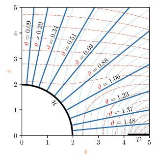
Figure 2: The solid blue lines represent some of the geodesic lines resolved by the numerical solver by starting from the horizon $\mathcal{H}$ at the angle ${\color[rgb]{1,0,0}{\vartheta}}$ ($\mathbin{\dot{=}}\,{\color[rgb]{1,.5,0}{\theta}}$) as shown next to the line. Light blue dashed lines represent the potential $\zeta$ and light red dash-dotted lines show $\psi$. The thick black line at ${\color[rgb]{1,.5,0}{\hat{z}}}=0$ is the disk $\mathcal{D}$.

While it is not obvious from the figure, the geodesics are, of course, deformed by the presence of the disk, the effect can be seen in greater detail in Fig. 11. Even the difference between the Weyl coordinates ${\color[rgb]{1,.5,0}{\hat{x}}}$ and ${\color[rgb]{1,.5,0}{\hat{z}}}$ and the Krishnan equivalents ${\color[rgb]{1,0,0}{\hat{X}}}$ and ${\color[rgb]{1,0,0}{\hat{Z}}}$, which have a similar definition except for a correction of $2{\color[rgb]{0.5,0.5,0}{M}}$ which removes the difference of choice of the value at the horizon.

$${\color[rgb]{1,0,0}{\hat{X}}} =({\color[rgb]{1,0,0}{s}}+2{\color[rgb]{0.5,0.5,0}{M}})\sin{\color[rgb]{1,0,0}{\vartheta}}\,, {\color[rgb]{1,0,0}{\hat{Z}}} =({\color[rgb]{1,0,0}{s}}+2{\color[rgb]{0.5,0.5,0}{M}})\cos{\color[rgb]{1,0,0}{\vartheta}}\,,$$

is only evident further away from the black hole, as can be seen in Fig. 3.

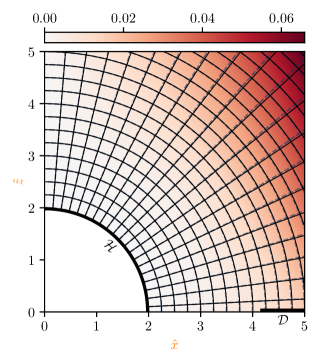
Figure 3: The Krishnan coordinates ${\color[rgb]{1,0,0}{s}}$ and ${\color[rgb]{1,0,0}{\vartheta}}$ in the region between the black hole and the disk are plotted in solid black lines while light blue dashed lines are the Weyl coordinates ${\color[rgb]{1,.5,0}{r}}$ and ${\color[rgb]{1,.5,0}{\theta}}$. The difference between the two coordinate systems, measured by $\sqrt{\left({\color[rgb]{1,.5,0}{\hat{x}}}-{\color[rgb]{1,0,0}{\hat{X}}}\right)^{2}+\left({\color[rgb]{1,.5,0}{\hat{z}}}-{\color[rgb]{1,0,0}{\hat{Z}}}\right)^{2}}$ , is shown by the saturation of the background.

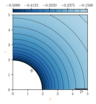
Figure 4: Spin coefficient ${\color[rgb]{0,0,1}{\mu}}$ (expansion of ${\color[rgb]{0,0,1}{n}}^{a}$) in the region between the black hole and the disk.

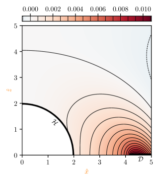
Figure 5: Spin coefficient ${\color[rgb]{0,0,1}{\lambda}}$ (shear of ${\color[rgb]{0,0,1}{n}}^{a}$) in the region between the black hole and the disk.

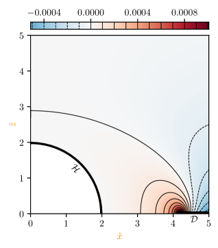
Figure 6: ${\color[rgb]{0,0,1}{\kern-1.00006pt\mathit{\Psi}\kern-0.80002pt}}_{0}$ in the region between the black hole and the disk.

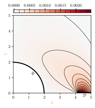
Figure 7: ${\color[rgb]{0,0,1}{\kern-1.00006pt\mathit{\Psi}\kern-0.80002pt}}_{1}$ in the region between the black hole and the disk.

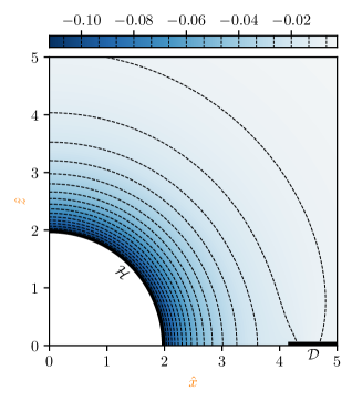
Figure 8: ${\color[rgb]{0,0,1}{\kern-1.00006pt\mathit{\Psi}\kern-0.80002pt}}_{2}$ in the region between the black hole and the disk.

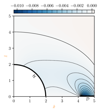
Figure 9: ${\color[rgb]{0,0,1}{\kern-1.00006pt\mathit{\Psi}\kern-0.80002pt}}_{3}$ in the region between the black hole and the disk.

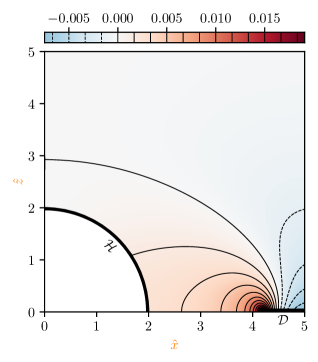
Figure 10: ${\color[rgb]{0,0,1}{\kern-1.00006pt\mathit{\Psi}\kern-0.80002pt}}_{4}$ in the region between the black hole and the disk.

V.1 NP scalars

In the following figures, the saturation of contour shading corresponds to the magnitude, while blue regions (with dashed contours) have negative values and red ones (with solid contours) positive ones. Zero saturation (white) denotes zero value (or the interior of the black hole). However, the (color) scale is not the same for all plots.

Let us start with the spin coefficients ${\color[rgb]{0,0,1}{\mu}}$ and ${\color[rgb]{0,0,1}{\lambda}}$ in Figs. 4 and 5 which represent the expansion and shear of the null congruence generated by ${\color[rgb]{0,0,1}{n}}^{a}$. Although the value is different, the profile of ${\color[rgb]{0,0,1}{\mu}}$ is almost the same as in the Schwarzschild case. On the other hand, ${\color[rgb]{0,0,1}{\lambda}}$ is no longer vanishing, as in Schwarzschild, and its value grows in the vicinity of the inner edge of the disk, where the density of the disk is the highest.

We shall proceed with the Weyl scalars, which can be found in Figs. 6 to 10. The presence of the disk deforms the geometry in such a way that all Weyl scalars are non-vanishing, and the magnitude of their deviation is highest in the vicinity of the disk. In the pure Schwarzschild, we have only ${\color[rgb]{0,0,1}{\kern-1.00006pt\mathit{\Psi}\kern-0.80002pt}}_{2}=-{\color[rgb]{0.5,0.5,0}{M}}/{\color[rgb]{1,0,0}{s}}^{3}$.

VI Analytic aspects of horizon geometry

In the previous section, we used a particular solution (120) of the Einstein equations and solved the geodesic equations for null rays providing the null tetrad vectors in this given space-time. By appropriate projections and derivatives, we obtained the IH/NP quantities. We already mentioned the possibility that, because it is much easier to obtain $\psi$ as solution of the linear Laplace equation than to find $\zeta$, we may, for a given $\psi$, solve (60b) to get $\zeta$ along the rays. Due to (61), we know $\zeta$ on the horizon which is the starting point of each ray.

In the IH formalism, the space-time geometry is determined by the geometry of the horizon and a few additional fields. It would thus be nice if we could, instead of choosing a given solution $\psi$ of the Laplace equation (51a), construct $\psi$ from the horizon geometry.

Under the assumption that the space-time is static, i.e., there exist Weyl coordinates in which the Laplace equation (51a) for $\psi$ holds. For this field equation, the horizon geometry then becomes the boundary condition. With such a construction, we can determine all space-time quantities from the horizon geometry. Indeed, this approach assumes time and axial symmetries of the space-time, which not only lead to the Laplace equation for $\psi$ but also determine ${\color[rgb]{0,0,1}{\kern-1.00006pt\mathit{\Psi}\kern-0.80002pt}}_{4}$ everywhere (and thus also on $\mathcal{N}_{0}$).

If the horizon geometry is given by the constant ${\color[rgb]{0.5,0.5,0}{\mathcal{R}}}$ and the function $h({\color[rgb]{1,0,0}{\varsigma}})$ appearing in (8) we may introduce the coordinate ${\color[rgb]{1,.5,0}{\theta}}$ so that ${\color[rgb]{1,0,0}{\varsigma}}=\cos{\color[rgb]{1,.5,0}{\theta}}$ and define

$$\tilde{\psi}({\color[rgb]{1,.5,0}{\theta}})=-\frac{1}{2}\log\!\left(\frac{h({\color[rgb]{1,0,0}{\varsigma}})}{\sin^{2}{\color[rgb]{1,.5,0}{\theta}}}\right).$$ (90)

Conditions (9) fix the value of $\tilde{\psi}({\color[rgb]{1,.5,0}{\theta}}=0)=\tilde{\psi}({\color[rgb]{1,.5,0}{\theta}}=\kern 0.39993pt\uppi\kern 0.39993pt)=0$.

Then the ${\color[rgb]{1,0,0}{u}}=\mathrm{constant}$ section of the (Killing) horizon is a topological sphere with

$$\mathrm{d}\mathscr{s}_{\SS_{0}}{}^{2}={\color[rgb]{0.5,0.5,0}{\mathcal{R}}}^{2}\left(\mathrm{e}^{2\hat{\psi}}\mathrm{d}{\color[rgb]{1,.5,0}{\theta}}^{2}+\mathrm{e}^{-2\hat{\psi}}\sin^{2}{\color[rgb]{1,.5,0}{\theta}}\,\mathrm{d}{\color[rgb]{1,.5,0}{\phi}}^{2}\right).$$ (91)

Due to the assumed form of ${\color[rgb]{0.5,0.5,0}{f}}=1-\frac{2{\color[rgb]{0.5,0.5,0}{M}}}{{\color[rgb]{1,.5,0}{r}}}$ we put ${\color[rgb]{1,.5,0}{r}}=2{\color[rgb]{0.5,0.5,0}{M}}$ at the horizon and from (61), we get

$$\begin{aligned} \psi({\color[rgb]{1,.5,0}{r}}=2{\color[rgb]{0.5,0.5,0}{M}},{\color[rgb]{1,.5,0}{\theta}})&=2\Big{(}\psi({\color[rgb]{1,.5,0}{r}}=2{\color[rgb]{0.5,0.5,0}{M}},{\color[rgb]{1,.5,0}{\theta}})-\psi_{\text{pole}}\Big{)}=\hat{\psi}({\color[rgb]{1,.5,0}{\theta}})\,,\\ {\color[rgb]{0.5,0.5,0}{M}}&=\tfrac{1}{2}{\color[rgb]{0.5,0.5,0}{\mathcal{R}}}\,\mathrm{e}^{\psi_{\text{pole}}}\,.\end{aligned}$$

The surface gravity is given by (80). Once we have determined ${\color[rgb]{0.5,0.5,0}{M}}$ and the function $\psi({\color[rgb]{1,.5,0}{r}}=2{\color[rgb]{0.5,0.5,0}{M}},{\color[rgb]{1,.5,0}{\theta}})$ on the horizon, we can write $\psi$ both at and outside the horizon as

$$\psi({\color[rgb]{1,.5,0}{r}},{\color[rgb]{1,.5,0}{\theta}})=\sum_{l}\psi_{l}\,P_{l}\!\left(\frac{{\color[rgb]{1,.5,0}{r}}}{{\color[rgb]{0.5,0.5,0}{M}}}-1\right)P_{l}(\cos{\color[rgb]{1,.5,0}{\theta}})\,,$$ (92)

where $P_{l}$ are the Legendre polynomials and $l=0,2,4,\dots$. This can be shown from the well-known form of the inner multipole expansion of the regular solution of the Laplace equation in the prolate spheroidal coordinates as well by a direct substitution into (60a). Because Legendre polynomials satisfy $P_{l}(1)=1$, the coefficients $\psi_{l}$ are given directly as the multipole expansion of the potential $\psi({\color[rgb]{1,.5,0}{r}}=2{\color[rgb]{0.5,0.5,0}{M}},{\color[rgb]{1,.5,0}{\theta}})$ on the horizon

$$\psi({\color[rgb]{1,.5,0}{r}}=2{\color[rgb]{0.5,0.5,0}{M}},{\color[rgb]{1,.5,0}{\theta}})=\sum_{l}\psi_{l}P_{l}(\cos{\color[rgb]{1,.5,0}{\theta}})\,.$$ (93)

When we specify $\psi$ on the horizon, Eq. (92) provides its extension outside the black hole. Obviously, it can hold only in the vacuum part of the space-time, and we will now demonstrate the imprint of the presence of matter on the analytic properties of the horizon geometry, which will be related to the convergence radius of the expansion (92). Due to its particular form, the values on the symmetry axis are directly related to those on the horizon

$$\psi({\color[rgb]{1,.5,0}{r}}=2{\color[rgb]{0.5,0.5,0}{M}},{\color[rgb]{1,.5,0}{\theta}})=\psi({\color[rgb]{1,.5,0}{z}}={\color[rgb]{0.5,0.5,0}{M}}\cos{\color[rgb]{1,.5,0}{\theta}},{\color[rgb]{1,.5,0}{\varrho}}=0)\,,$$ (94)

where ${\color[rgb]{1,.5,0}{\varrho}},{\color[rgb]{1,.5,0}{z}}$ are the cylindrical Weyl coordinates (53). The convergence is obvious for $|{\color[rgb]{1,.5,0}{z}}|\leq{\color[rgb]{0.5,0.5,0}{M}}$, because the transformation (53) maps the horizon on the linear interval on the ${\color[rgb]{1,.5,0}{z}}$ axis. But if we investigate the convergence outside the horizon, this relation says that $\psi_{l}$ has to fall off quickly enough so that $\sum_{l}\psi_{l}P_{l}({\color[rgb]{1,.5,0}{z}}/{\color[rgb]{0.5,0.5,0}{M}})$ converges also for $|{\color[rgb]{1,.5,0}{z}}|>{\color[rgb]{0.5,0.5,0}{M}}$. Thus, because the convergence criteria of $\sum a_{l}P_{l}(\cos{\color[rgb]{1,.5,0}{\theta}})$ and $\sum a_{l}$ are the same (e.g. $\lim_{n\to\infty}|a_{l}|^{1/l}\leq 1$), if $\sum_{l}\psi_{l}P_{l}({\color[rgb]{1,.5,0}{z}}/{\color[rgb]{0.5,0.5,0}{M}})$ converges for $|{\color[rgb]{1,.5,0}{z}}|<{\color[rgb]{1,.5,0}{z}}_{\text{max}}$, Eq. (92) converges for ${\color[rgb]{1,.5,0}{r}}<{\color[rgb]{1,.5,0}{z}}_{\text{max}}+{\color[rgb]{0.5,0.5,0}{M}}$.

Using ${\color[rgb]{1,0,0}{\varsigma}}=\cos{\color[rgb]{1,.5,0}{\theta}}$ again, if the real convergence radius of the Legendre series for

$$\psi_{\mathcal{H}}({\color[rgb]{1,0,0}{\varsigma}})=\sum_{l}\psi_{l}\,P_{l}({\color[rgb]{1,0,0}{\varsigma}})$$ (95)

is ${\color[rgb]{1,0,0}{\varsigma}}_{\text{max}}>1$, we know that (92) will converge for ${\color[rgb]{1,.5,0}{r}}<{\color[rgb]{1,.5,0}{r}}_{\text{max}}$, where

$${\color[rgb]{1,.5,0}{r}}_{\text{max}}\equiv{\color[rgb]{0.5,0.5,0}{M}}(1+{\color[rgb]{1,0,0}{\varsigma}}_{\text{max}})>2{\color[rgb]{0.5,0.5,0}{M}}\,,$$ (96)

because $|P_{l}(\cos{\color[rgb]{1,.5,0}{\theta}})|\leq 1$.

For the considered disk perturbation $\psi$ we have

$$\begin{aligned} \psi_{\mathcal{H}}({\color[rgb]{1,0,0}{\varsigma}})&=\frac{2{\color[rgb]{0.5,0.5,0}{\mathcal{M}}}}{3\kern 0.39993pt\uppi\kern 0.39993pt{\color[rgb]{0.5,0.5,0}{M}}{\color[rgb]{1,0,0}{\varsigma}}^{5}}\Big{(}5{\color[rgb]{0.5,0.5,0}{\mathsfit{b}}}{\color[rgb]{1,0,0}{\varsigma}}^{3}+3{\color[rgb]{0.5,0.5,0}{\mathsfit{b}}}^{3}{\color[rgb]{1,0,0}{\varsigma}}\\ &\qquad{}-3\left({\color[rgb]{0.5,0.5,0}{\mathsfit{b}}}^{2}+{\color[rgb]{1,0,0}{\varsigma}}^{2}\right)^{2}\arctan\frac{{\color[rgb]{1,0,0}{\varsigma}}}{{\color[rgb]{0.5,0.5,0}{\mathsfit{b}}}}\Big{)},\end{aligned}$$

where ${\color[rgb]{0.5,0.5,0}{\mathsfit{b}}}={\color[rgb]{0.5,0.5,0}{b}}/{\color[rgb]{0.5,0.5,0}{M}}$ and the value of ${\color[rgb]{1,0,0}{\varsigma}}_{\text{max}}=\sqrt{{\color[rgb]{0.5,0.5,0}{\mathsfit{b}}}^{2}+1}$ for this function is known for its Chebyshev expansion because the $\arctan$ function is the well-known showcase in the theory of approximations, [32]. The same value of ${\color[rgb]{1,0,0}{\varsigma}}_{\text{max}}$ is also valid for the Legendre series, which share the same Bernstein ellipse that determines the exponential fall-off of the expansion coefficients $\psi_{l}$, [33]. But because the ratio of Legendre and Chebyshev polynomials has

$$\lim_{l\to\infty}\left|\frac{P_{l}(s)}{T_{l}(s)}\right|^{1/l}=1\,,$$ (97)

for $s>1$, also the series (92) will converge for $2{\color[rgb]{0.5,0.5,0}{M}}\leq{\color[rgb]{1,.5,0}{r}}<{\color[rgb]{1,.5,0}{r}}_{\text{max}}$. For the potential studied, the value of

$${\color[rgb]{1,.5,0}{r}}_{\text{max}}={\color[rgb]{0.5,0.5,0}{M}}+\sqrt{{\color[rgb]{0.5,0.5,0}{M}}^{2}+{\color[rgb]{0.5,0.5,0}{b}}^{2}}$$ (98)

is equal to the inner radius of the disk.

Let us summarize this finding. The geometry of the horizon influenced by the external matter is specified by a single function $\psi_{\mathcal{H}}({\color[rgb]{1,0,0}{\varsigma}})$, where ${\color[rgb]{1,0,0}{\varsigma}}=\cos{\color[rgb]{1,.5,0}{\theta}}$, and therefore belongs to the interval $[-1,1]$. However, the analytic properties of the horizon geometry allow summation up to ${\color[rgb]{1,0,0}{\varsigma}}_{\text{max}}>1$, and this value directly determines the region where we can construct the set of space-time quantities starting with $\psi$ given by (92). For the considered exact solution of superimposed fields (120) taken from [23] we then see that this region of space-time recovered from the horizon geometry (and symmetry assumptions) is $2{\color[rgb]{0.5,0.5,0}{M}}\leq{\color[rgb]{1,.5,0}{r}}<{\color[rgb]{1,.5,0}{r}}_{\text{max}}$ where ${\color[rgb]{1,.5,0}{r}}_{\text{max}}$ is the inner radius of the disk.

VII Conclusion

The isolated horizons framework allows for a quasi-local description of deformed black holes in equilibrium, but the involved equations are quite complicated. We have shown how, in spherical symmetry, these equations and gauge conditions imply the initial data leading to the Schwarzschild space-time. Then we considered axisymmetric initial data and found the geometry of a static space-time surrounding the horizon in the form of a series expansion of NP quantities in the neighborhood of the horizon. Although the solution was found only up to a finite order of expansion, this solution will reflect the changes of the geometry due to the presence of external matter. Moreover, we solved the same problem numerically for one particular example in the form of a simplified model of an accretion disk (inverted Morgan–Morgan disk) and discussed the convergence of both solutions. The numerical solution also enabled us to plot the most interesting NP scalars.

Since we followed the same basic procedure, we arrived at similar series expansions as in [15]. However, while those in [15] represent a general solution and do not give any clues for the right choice of the initial data for any specific space-time. The expansions we have found represent one particular choice which has been illustrated in the figures. While we have used one particular disk for these illustrations, any suitable solution could be used. Since the function $\zeta$ is not always available as an analytical solution, it is convenient that it can be obtained from the horizon geometry together with NP quantities.

Appendix A Newman–Penrose formalism

We only briefly review the Newman–Penrose formalism with emphasis on the relations we shall need. For a more in-depth review of the formalism, see [16].

The NP null tetrad consists of four null vectors ${\color[rgb]{0,0,1}{\ell\kern 0.20004pt}}^{a},{\color[rgb]{0,0,1}{n}}^{a},{\color[rgb]{0,0,1}{m}}^{a}$ and $\mkern 2.0mu\overline{\mkern-2.0mu{\color[rgb]{0,0,1}{m}}\mkern-0.7mu}\mkern 0.7mu^{a}$ normalized by the conditions

$${\color[rgb]{0,0,1}{\ell\kern 0.20004pt}}^{a}\,{\color[rgb]{0,0,1}{n}}_{a} =1\,, {\color[rgb]{0,0,1}{m}}^{a}\,\mkern 2.0mu\overline{\mkern-2.0mu{\color[rgb]{0,0,1}{m}}\mkern-0.7mu}\mkern 0.7mu_{a} =-1\,,$$

while all remaining contractions vanish. These vectors constitute the basis of the tangent space, so that any tensor can be expanded in terms of them. We employ the convention that any real vector $X^{a}$ has the decomposition

$$X^{a}=X_{0}\,{\color[rgb]{0,0,1}{\ell\kern 0.20004pt}}^{a}+X_{1}\,{\color[rgb]{0,0,1}{n}}^{a}+X_{2}\,{\color[rgb]{0,0,1}{m}}^{a}+\mkern 2.0mu\overline{\mkern-2.0muX\mkern-0.7mu}\mkern 0.7mu_{2}\,\mkern 2.0mu\overline{\mkern-2.0mu{\color[rgb]{0,0,1}{m}}\mkern-0.7mu}\mkern 0.7mu^{a}\,.$$ (99)

The metric tensor in terms of the null tetrad reads

$$g_{ab}=2\,{\color[rgb]{0,0,1}{\ell\kern 0.20004pt}}_{(a}\,{\color[rgb]{0,0,1}{n}}_{b)}-2\,{\color[rgb]{0,0,1}{m}}_{(a}\mkern 2.0mu\overline{\mkern-2.0mu{\color[rgb]{0,0,1}{m}}\mkern-0.7mu}\mkern 0.7mu_{b)}\,,$$ (100)

where the parentheses denote symmetrization.

In the NP formalism, the spin coefficients are the Ricci rotation coefficients with respect to the null tetrad $\left({\color[rgb]{0,0,1}{\ell\kern 0.20004pt}}^{a},{\color[rgb]{0,0,1}{n}}^{a},{\color[rgb]{0,0,1}{m}}^{a},\mkern 2.0mu\overline{\mkern-2.0mu{\color[rgb]{0,0,1}{m}}\mkern-0.7mu}\mkern 0.7mu^{a}\right)$ and they encode the connection. The twelve independent complex coefficients are defined by

(106)

where

$${\color[rgb]{0,0,1}{\mathrm{D}}} ={\color[rgb]{0,0,1}{\ell\kern 0.20004pt}}^{a}\nabla_{a}\,, {\color[rgb]{0,0,1}{\Delta}} ={\color[rgb]{0,0,1}{n}}^{a}\nabla_{a}\,,$$

$${\color[rgb]{0,0,1}{\updelta}} ={\color[rgb]{0,0,1}{m}}^{a}\nabla_{a}\,, \mkern 2.0mu\overline{\mkern-2.0mu{\color[rgb]{0,0,1}{\updelta}}\mkern-0.7mu}\mkern 0.7mu =\mkern 2.0mu\overline{\mkern-2.0mu{\color[rgb]{0,0,1}{m}}\mkern-0.7mu}\mkern 0.7mu^{a}\nabla_{a}\,.$$

Using the operators, we can find how the tetrad vectors change along each other. The expressions, called transport equations, are:

$$\begin{aligned} {\color[rgb]{0,0,1}{\mathrm{D}}}{\color[rgb]{0,0,1}{\ell\kern 0.20004pt}}^{a}&=\left({\color[rgb]{0,0,1}{\varepsilon}}+\mkern 2.0mu\overline{\mkern-2.0mu{\color[rgb]{0,0,1}{\varepsilon}}\mkern-0.7mu}\mkern 0.7mu\right){\color[rgb]{0,0,1}{\ell\kern 0.20004pt}}^{a}-\mkern 2.0mu\overline{\mkern-2.0mu{\color[rgb]{0,0,1}{\kappa}}\mkern-0.7mu}\mkern 0.7mu\,{\color[rgb]{0,0,1}{m}}^{a}-{\color[rgb]{0,0,1}{\kappa}}\,\mkern 2.0mu\overline{\mkern-2.0mu{\color[rgb]{0,0,1}{m}}\mkern-0.7mu}\mkern 0.7mu^{a}\,,\\ {\color[rgb]{0,0,1}{\Delta}}{\color[rgb]{0,0,1}{\ell\kern 0.20004pt}}^{a}&=\left({\color[rgb]{0,0,1}{\gamma}}+\mkern 2.0mu\overline{\mkern-2.0mu{\color[rgb]{0,0,1}{\gamma}}\mkern-0.7mu}\mkern 0.7mu\right){\color[rgb]{0,0,1}{\ell\kern 0.20004pt}}^{a}-\mkern 2.0mu\overline{\mkern-2.0mu{\color[rgb]{0,0,1}{\tau}}\mkern-0.7mu}\mkern 0.7mu\,{\color[rgb]{0,0,1}{m}}^{a}-{\color[rgb]{0,0,1}{\tau}}\,\mkern 2.0mu\overline{\mkern-2.0mu{\color[rgb]{0,0,1}{m}}\mkern-0.7mu}\mkern 0.7mu^{a}\,,\\ {\color[rgb]{0,0,1}{\updelta}}{\color[rgb]{0,0,1}{\ell\kern 0.20004pt}}^{a}&=\left(\mkern 2.0mu\overline{\mkern-2.0mu{\color[rgb]{0,0,1}{\alpha}}\mkern-0.7mu}\mkern 0.7mu+{\color[rgb]{0,0,1}{\beta}}\right){\color[rgb]{0,0,1}{\ell\kern 0.20004pt}}^{a}-\mkern 2.0mu\overline{\mkern-2.0mu{\color[rgb]{0,0,1}{\rho}}\mkern-0.7mu}\mkern 0.7mu\,{\color[rgb]{0,0,1}{m}}^{a}-{\color[rgb]{0,0,1}{\sigma}}\,\mkern 2.0mu\overline{\mkern-2.0mu{\color[rgb]{0,0,1}{m}}\mkern-0.7mu}\mkern 0.7mu^{a}\,,\\ {\color[rgb]{0,0,1}{\mathrm{D}}}{\color[rgb]{0,0,1}{n}}^{a}&=-\left({\color[rgb]{0,0,1}{\varepsilon}}+\mkern 2.0mu\overline{\mkern-2.0mu{\color[rgb]{0,0,1}{\varepsilon}}\mkern-0.7mu}\mkern 0.7mu\right){\color[rgb]{0,0,1}{n}}^{a}+{\color[rgb]{0,0,1}{\pi}}\,{\color[rgb]{0,0,1}{m}}^{a}+\mkern 2.0mu\overline{\mkern-2.0mu{\color[rgb]{0,0,1}{\pi}}\mkern-0.7mu}\mkern 0.7mu\,\mkern 2.0mu\overline{\mkern-2.0mu{\color[rgb]{0,0,1}{m}}\mkern-0.7mu}\mkern 0.7mu^{a}\,,\\ {\color[rgb]{0,0,1}{\Delta}}{\color[rgb]{0,0,1}{n}}^{a}&=-\left({\color[rgb]{0,0,1}{\gamma}}+\mkern 2.0mu\overline{\mkern-2.0mu{\color[rgb]{0,0,1}{\gamma}}\mkern-0.7mu}\mkern 0.7mu\right){\color[rgb]{0,0,1}{n}}^{a}+{\color[rgb]{0,0,1}{\nu}}\,{\color[rgb]{0,0,1}{m}}^{a}+\mkern 2.0mu\overline{\mkern-2.0mu{\color[rgb]{0,0,1}{\nu}}\mkern-0.7mu}\mkern 0.7mu\,\mkern 2.0mu\overline{\mkern-2.0mu{\color[rgb]{0,0,1}{m}}\mkern-0.7mu}\mkern 0.7mu^{a}\,,\\ {\color[rgb]{0,0,1}{\updelta}}{\color[rgb]{0,0,1}{n}}^{a}&=-(\mkern 2.0mu\overline{\mkern-2.0mu{\color[rgb]{0,0,1}{\alpha}}\mkern-0.7mu}\mkern 0.7mu+{\color[rgb]{0,0,1}{\beta}}){\color[rgb]{0,0,1}{n}}^{a}+{\color[rgb]{0,0,1}{\mu}}\,{\color[rgb]{0,0,1}{m}}^{a}+\mkern 2.0mu\overline{\mkern-2.0mu{\color[rgb]{0,0,1}{\lambda}}\mkern-0.7mu}\mkern 0.7mu\,\mkern 2.0mu\overline{\mkern-2.0mu{\color[rgb]{0,0,1}{m}}\mkern-0.7mu}\mkern 0.7mu^{a}\,,\\ {\color[rgb]{0,0,1}{\mathrm{D}}}{\color[rgb]{0,0,1}{m}}^{a}&=\mkern 2.0mu\overline{\mkern-2.0mu{\color[rgb]{0,0,1}{\pi}}\mkern-0.7mu}\mkern 0.7mu\,{\color[rgb]{0,0,1}{\ell\kern 0.20004pt}}^{a}-{\color[rgb]{0,0,1}{\kappa}}\,{\color[rgb]{0,0,1}{n}}^{a}+\left({\color[rgb]{0,0,1}{\varepsilon}}-\mkern 2.0mu\overline{\mkern-2.0mu{\color[rgb]{0,0,1}{\varepsilon}}\mkern-0.7mu}\mkern 0.7mu\right){\color[rgb]{0,0,1}{m}}^{a}\,,\\ {\color[rgb]{0,0,1}{\Delta}}{\color[rgb]{0,0,1}{m}}^{a}&=\mkern 2.0mu\overline{\mkern-2.0mu{\color[rgb]{0,0,1}{\nu}}\mkern-0.7mu}\mkern 0.7mu\,{\color[rgb]{0,0,1}{\ell\kern 0.20004pt}}^{a}-{\color[rgb]{0,0,1}{\tau}}\,{\color[rgb]{0,0,1}{n}}^{a}+\left({\color[rgb]{0,0,1}{\gamma}}-\mkern 2.0mu\overline{\mkern-2.0mu{\color[rgb]{0,0,1}{\gamma}}\mkern-0.7mu}\mkern 0.7mu\right){\color[rgb]{0,0,1}{m}}^{a}\,,\\ {\color[rgb]{0,0,1}{\updelta}}{\color[rgb]{0,0,1}{m}}^{a}&=\mkern 2.0mu\overline{\mkern-2.0mu{\color[rgb]{0,0,1}{\lambda}}\mkern-0.7mu}\mkern 0.7mu\,{\color[rgb]{0,0,1}{\ell\kern 0.20004pt}}^{a}-{\color[rgb]{0,0,1}{\sigma}}\,{\color[rgb]{0,0,1}{n}}^{a}+\left({\color[rgb]{0,0,1}{\beta}}-\mkern 2.0mu\overline{\mkern-2.0mu{\color[rgb]{0,0,1}{\alpha}}\mkern-0.7mu}\mkern 0.7mu\right){\color[rgb]{0,0,1}{m}}^{a}\,,\\ \mkern 2.0mu\overline{\mkern-2.0mu{\color[rgb]{0,0,1}{\updelta}}\mkern-0.7mu}\mkern 0.7mu{\color[rgb]{0,0,1}{m}}^{a}&=\mkern 2.0mu\overline{\mkern-2.0mu{\color[rgb]{0,0,1}{\mu}}\mkern-0.7mu}\mkern 0.7mu\,{\color[rgb]{0,0,1}{\ell\kern 0.20004pt}}^{a}-{\color[rgb]{0,0,1}{\rho}}\,{\color[rgb]{0,0,1}{n}}^{a}+\left({\color[rgb]{0,0,1}{\alpha}}-\mkern 2.0mu\overline{\mkern-2.0mu{\color[rgb]{0,0,1}{\beta}}\mkern-0.7mu}\mkern 0.7mu\right){\color[rgb]{0,0,1}{m}}^{a}\,.\end{aligned}$$

Acting on a scalar, the operators ${\color[rgb]{0,0,1}{\mathrm{D}}}$, ${\color[rgb]{0,0,1}{\Delta}}$, and ${\color[rgb]{0,0,1}{\updelta}}$ obey the commutation relations:

$$\begin{aligned} {\color[rgb]{0,0,1}{\mathrm{D}}}{\color[rgb]{0,0,1}{\updelta}}-{\color[rgb]{0,0,1}{\updelta}}{\color[rgb]{0,0,1}{\mathrm{D}}}&=(\mkern 2.0mu\overline{\mkern-2.0mu{\color[rgb]{0,0,1}{\pi}}\mkern-0.7mu}\mkern 0.7mu-\mkern 2.0mu\overline{\mkern-2.0mu{\color[rgb]{0,0,1}{\alpha}}\mkern-0.7mu}\mkern 0.7mu-{\color[rgb]{0,0,1}{\beta}}){\color[rgb]{0,0,1}{\mathrm{D}}}-{\color[rgb]{0,0,1}{\kappa}}{\color[rgb]{0,0,1}{\Delta}}\\ &\qquad{}+(\mkern 2.0mu\overline{\mkern-2.0mu{\color[rgb]{0,0,1}{\rho}}\mkern-0.7mu}\mkern 0.7mu-\mkern 2.0mu\overline{\mkern-2.0mu{\color[rgb]{0,0,1}{\varepsilon}}\mkern-0.7mu}\mkern 0.7mu+{\color[rgb]{0,0,1}{\varepsilon}}){\color[rgb]{0,0,1}{\updelta}}+{\color[rgb]{0,0,1}{\sigma}}\mkern 2.0mu\overline{\mkern-2.0mu{\color[rgb]{0,0,1}{\updelta}}\mkern-0.7mu}\mkern 0.7mu\,,\\ {\color[rgb]{0,0,1}{\Delta}}{\color[rgb]{0,0,1}{\mathrm{D}}}-{\color[rgb]{0,0,1}{\mathrm{D}}}{\color[rgb]{0,0,1}{\Delta}}&=({\color[rgb]{0,0,1}{\gamma}}+\mkern 2.0mu\overline{\mkern-2.0mu{\color[rgb]{0,0,1}{\gamma}}\mkern-0.7mu}\mkern 0.7mu){\color[rgb]{0,0,1}{\mathrm{D}}}+({\color[rgb]{0,0,1}{\varepsilon}}+\mkern 2.0mu\overline{\mkern-2.0mu{\color[rgb]{0,0,1}{\varepsilon}}\mkern-0.7mu}\mkern 0.7mu){\color[rgb]{0,0,1}{\Delta}}\\ &\qquad{}-(\mkern 2.0mu\overline{\mkern-2.0mu{\color[rgb]{0,0,1}{\tau}}\mkern-0.7mu}\mkern 0.7mu+{\color[rgb]{0,0,1}{\pi}}){\color[rgb]{0,0,1}{\updelta}}-({\color[rgb]{0,0,1}{\tau}}+\mkern 2.0mu\overline{\mkern-2.0mu{\color[rgb]{0,0,1}{\pi}}\mkern-0.7mu}\mkern 0.7mu)\mkern 2.0mu\overline{\mkern-2.0mu{\color[rgb]{0,0,1}{\updelta}}\mkern-0.7mu}\mkern 0.7mu\,,\\ {\color[rgb]{0,0,1}{\Delta}}{\color[rgb]{0,0,1}{\updelta}}-{\color[rgb]{0,0,1}{\updelta}}{\color[rgb]{0,0,1}{\Delta}}&=\mkern 2.0mu\overline{\mkern-2.0mu{\color[rgb]{0,0,1}{\nu}}\mkern-0.7mu}\mkern 0.7mu{\color[rgb]{0,0,1}{\mathrm{D}}}+(\mkern 2.0mu\overline{\mkern-2.0mu{\color[rgb]{0,0,1}{\alpha}}\mkern-0.7mu}\mkern 0.7mu+{\color[rgb]{0,0,1}{\beta}}-{\color[rgb]{0,0,1}{\tau}}){\color[rgb]{0,0,1}{\Delta}}\\ &\qquad{}+({\color[rgb]{0,0,1}{\gamma}}-\mkern 2.0mu\overline{\mkern-2.0mu{\color[rgb]{0,0,1}{\gamma}}\mkern-0.7mu}\mkern 0.7mu-{\color[rgb]{0,0,1}{\mu}}){\color[rgb]{0,0,1}{\updelta}}-\mkern 2.0mu\overline{\mkern-2.0mu{\color[rgb]{0,0,1}{\lambda}}\mkern-0.7mu}\mkern 0.7mu\mkern 2.0mu\overline{\mkern-2.0mu{\color[rgb]{0,0,1}{\updelta}}\mkern-0.7mu}\mkern 0.7mu\,,\\ {\color[rgb]{0,0,1}{\updelta}}\mkern 2.0mu\overline{\mkern-2.0mu{\color[rgb]{0,0,1}{\updelta}}\mkern-0.7mu}\mkern 0.7mu-\mkern 2.0mu\overline{\mkern-2.0mu{\color[rgb]{0,0,1}{\updelta}}\mkern-0.7mu}\mkern 0.7mu{\color[rgb]{0,0,1}{\updelta}}&=({\color[rgb]{0,0,1}{\mu}}-\mkern 2.0mu\overline{\mkern-2.0mu{\color[rgb]{0,0,1}{\mu}}\mkern-0.7mu}\mkern 0.7mu){\color[rgb]{0,0,1}{\mathrm{D}}}+({\color[rgb]{0,0,1}{\rho}}-\mkern 2.0mu\overline{\mkern-2.0mu{\color[rgb]{0,0,1}{\rho}}\mkern-0.7mu}\mkern 0.7mu){\color[rgb]{0,0,1}{\Delta}}\\ &\qquad{}+(\mkern 2.0mu\overline{\mkern-2.0mu{\color[rgb]{0,0,1}{\alpha}}\mkern-0.7mu}\mkern 0.7mu-{\color[rgb]{0,0,1}{\beta}})\mkern 2.0mu\overline{\mkern-2.0mu{\color[rgb]{0,0,1}{\updelta}}\mkern-0.7mu}\mkern 0.7mu-({\color[rgb]{0,0,1}{\alpha}}-\mkern 2.0mu\overline{\mkern-2.0mu{\color[rgb]{0,0,1}{\beta}}\mkern-0.7mu}\mkern 0.7mu){\color[rgb]{0,0,1}{\updelta}}\,.\end{aligned}$$ (107)

Since all quantities in the NP formalism are projected onto the tetrad, except for the spin coefficients, we need also 5 non-zero complex components of the Weyl tensor

$$\begin{aligned} {\color[rgb]{0,0,1}{\kern-1.00006pt\mathit{\Psi}\kern-0.80002pt}}_{0}&=C_{abcd}\,{\color[rgb]{0,0,1}{\ell\kern 0.20004pt}}^{a}\,{\color[rgb]{0,0,1}{m}}^{b}\,{\color[rgb]{0,0,1}{\ell\kern 0.20004pt}}^{c}\,{\color[rgb]{0,0,1}{m}}^{d}\,,\\ {\color[rgb]{0,0,1}{\kern-1.00006pt\mathit{\Psi}\kern-0.80002pt}}_{1}&=C_{abcd}\,{\color[rgb]{0,0,1}{\ell\kern 0.20004pt}}^{a}\,{\color[rgb]{0,0,1}{n}}^{b}\,{\color[rgb]{0,0,1}{\ell\kern 0.20004pt}}^{c}\,{\color[rgb]{0,0,1}{m}}^{d}\,,\\ {\color[rgb]{0,0,1}{\kern-1.00006pt\mathit{\Psi}\kern-0.80002pt}}_{2}&=C_{abcd}\,{\color[rgb]{0,0,1}{\ell\kern 0.20004pt}}^{a}\,{\color[rgb]{0,0,1}{m}}^{b}\,\mkern 2.0mu\overline{\mkern-2.0mu{\color[rgb]{0,0,1}{m}}\mkern-0.7mu}\mkern 0.7mu^{c}\,{\color[rgb]{0,0,1}{n}}^{d}\,,\\ {\color[rgb]{0,0,1}{\kern-1.00006pt\mathit{\Psi}\kern-0.80002pt}}_{3}&=C_{abcd}\,{\color[rgb]{0,0,1}{\ell\kern 0.20004pt}}^{a}\,{\color[rgb]{0,0,1}{n}}^{b}\,\mkern 2.0mu\overline{\mkern-2.0mu{\color[rgb]{0,0,1}{m}}\mkern-0.7mu}\mkern 0.7mu^{c}\,{\color[rgb]{0,0,1}{n}}^{d}\,,\\ {\color[rgb]{0,0,1}{\kern-1.00006pt\mathit{\Psi}\kern-0.80002pt}}_{4}&=C_{abcd}\,\mkern 2.0mu\overline{\mkern-2.0mu{\color[rgb]{0,0,1}{m}}\mkern-0.7mu}\mkern 0.7mu^{a}\,{\color[rgb]{0,0,1}{n}}^{b}\,\mkern 2.0mu\overline{\mkern-2.0mu{\color[rgb]{0,0,1}{m}}\mkern-0.7mu}\mkern 0.7mu^{c}\,{\color[rgb]{0,0,1}{n}}^{d}\,,\end{aligned}$$

and 6 independent components of the Ricci tensor

$${\color[rgb]{0,0,1}{\kern-0.80002pt\mathit{\Phi}\kern-0.39993pt}}_{00} =-\frac{1}{2}R_{ab}\,{\color[rgb]{0,0,1}{\ell\kern 0.20004pt}}^{a}\,{\color[rgb]{0,0,1}{\ell\kern 0.20004pt}}^{b}\,,$$

$${\color[rgb]{0,0,1}{\kern-0.80002pt\mathit{\Phi}\kern-0.39993pt}}_{01} =-\frac{1}{2}R_{ab}\,{\color[rgb]{0,0,1}{\ell\kern 0.20004pt}}^{a}\,{\color[rgb]{0,0,1}{m}}^{b}\,,$$

$${\color[rgb]{0,0,1}{\kern-0.80002pt\mathit{\Phi}\kern-0.39993pt}}_{02} =-\frac{1}{2}R_{ab}\,{\color[rgb]{0,0,1}{m}}^{a}\,{\color[rgb]{0,0,1}{m}}^{b}\,,$$

$${\color[rgb]{0,0,1}{\kern-0.80002pt\mathit{\Phi}\kern-0.39993pt}}_{11} =-\frac{1}{2}R_{ab}\left({\color[rgb]{0,0,1}{\ell\kern 0.20004pt}}^{a}\,{\color[rgb]{0,0,1}{n}}^{b}+{\color[rgb]{0,0,1}{m}}^{a}\,\mkern 2.0mu\overline{\mkern-2.0mu{\color[rgb]{0,0,1}{m}}\mkern-0.7mu}\mkern 0.7mu^{b}\right),$$

$${\color[rgb]{0,0,1}{\kern-0.80002pt\mathit{\Phi}\kern-0.39993pt}}_{12} =-\frac{1}{2}R_{ab}\,{\color[rgb]{0,0,1}{n}}^{a}\,{\color[rgb]{0,0,1}{m}}^{b}\,,$$

$${\color[rgb]{0,0,1}{\kern-0.80002pt\mathit{\Phi}\kern-0.39993pt}}_{22} =-\frac{1}{2}R_{ab}\,{\color[rgb]{0,0,1}{n}}^{a}\,{\color[rgb]{0,0,1}{n}}^{b}\,.$$

where the components with switched indices are complex conjugates, ${\color[rgb]{0,0,1}{\kern-0.80002pt\mathit{\Phi}\kern-0.39993pt}}_{ba}=\mkern 2.0mu\overline{\mkern-2.0mu{\color[rgb]{0,0,1}{\kern-0.80002pt\mathit{\Phi}\kern-0.39993pt}}\mkern-0.7mu}\mkern 0.7mu_{ab}$. The trace of the Ricci tensor is given by the scalar curvature which in NP formalism is denoted by ${\color[rgb]{0,0,1}{\kern-0.80002pt\mathit{\Lambda}}}=\frac{R}{24}$.

A.1 Ricci identities

Since Einstein’s equations in NP formalism are just algebraic relations between NP quantities, the true field equations are provided by the Ricci and Bianchi identities. By the Ricci identities we mean the definition of the Riemann tensor,

$$\begin{aligned} 2\nabla_{[c}\nabla_{d]}\,X^{a}=-R^{a}{}_{bcd}\,X^{b}\,.\end{aligned}$$

Substituting the vectors of the null tetrad for $X_{a}$ and projecting them onto the null tetrad, these identities become differential equations for the spin coefficients.

$${\color[rgb]{0,0,1}{\mathrm{D}}}{\color[rgb]{0,0,1}{\rho}}-\mkern 2.0mu\overline{\mkern-2.0mu{\color[rgb]{0,0,1}{\updelta}}\mkern-0.7mu}\mkern 0.7mu{\color[rgb]{0,0,1}{\kappa}} ={\color[rgb]{0,0,1}{\rho}}^{2}+\left({\color[rgb]{0,0,1}{\varepsilon}}+\mkern 2.0mu\overline{\mkern-2.0mu{\color[rgb]{0,0,1}{\varepsilon}}\mkern-0.7mu}\mkern 0.7mu\right){\color[rgb]{0,0,1}{\rho}}-{\color[rgb]{0,0,1}{\kappa}}\left(3{\color[rgb]{0,0,1}{\alpha}}+\mkern 2.0mu\overline{\mkern-2.0mu{\color[rgb]{0,0,1}{\beta}}\mkern-0.7mu}\mkern 0.7mu-{\color[rgb]{0,0,1}{\pi}}\right)-{\color[rgb]{0,0,1}{\tau}}\mkern 2.0mu\overline{\mkern-2.0mu{\color[rgb]{0,0,1}{\kappa}}\mkern-0.7mu}\mkern 0.7mu+{\color[rgb]{0,0,1}{\sigma}}\mkern 2.0mu\overline{\mkern-2.0mu{\color[rgb]{0,0,1}{\sigma}}\mkern-0.7mu}\mkern 0.7mu+{\color[rgb]{0,0,1}{\kern-0.80002pt\mathit{\Phi}\kern-0.39993pt}}_{00}\,,$$ (108a)

$${\color[rgb]{0,0,1}{\mathrm{D}}}{\color[rgb]{0,0,1}{\sigma}}-{\color[rgb]{0,0,1}{\updelta}}{\color[rgb]{0,0,1}{\kappa}} =({\color[rgb]{0,0,1}{\rho}}+\mkern 2.0mu\overline{\mkern-2.0mu{\color[rgb]{0,0,1}{\rho}}\mkern-0.7mu}\mkern 0.7mu+3{\color[rgb]{0,0,1}{\varepsilon}}-\mkern 2.0mu\overline{\mkern-2.0mu{\color[rgb]{0,0,1}{\varepsilon}}\mkern-0.7mu}\mkern 0.7mu){\color[rgb]{0,0,1}{\sigma}}-({\color[rgb]{0,0,1}{\tau}}-\mkern 2.0mu\overline{\mkern-2.0mu{\color[rgb]{0,0,1}{\pi}}\mkern-0.7mu}\mkern 0.7mu+\mkern 2.0mu\overline{\mkern-2.0mu{\color[rgb]{0,0,1}{\alpha}}\mkern-0.7mu}\mkern 0.7mu+3{\color[rgb]{0,0,1}{\beta}}){\color[rgb]{0,0,1}{\kappa}}+{\color[rgb]{0,0,1}{\kern-1.00006pt\mathit{\Psi}\kern-0.80002pt}}_{0}\,,$$ (108b)

$${\color[rgb]{0,0,1}{\mathrm{D}}}{\color[rgb]{0,0,1}{\tau}}-{\color[rgb]{0,0,1}{\Delta}}{\color[rgb]{0,0,1}{\kappa}} ={\color[rgb]{0,0,1}{\rho}}({\color[rgb]{0,0,1}{\tau}}+\mkern 2.0mu\overline{\mkern-2.0mu{\color[rgb]{0,0,1}{\pi}}\mkern-0.7mu}\mkern 0.7mu)+{\color[rgb]{0,0,1}{\sigma}}(\mkern 2.0mu\overline{\mkern-2.0mu{\color[rgb]{0,0,1}{\tau}}\mkern-0.7mu}\mkern 0.7mu+{\color[rgb]{0,0,1}{\pi}})+({\color[rgb]{0,0,1}{\varepsilon}}-\mkern 2.0mu\overline{\mkern-2.0mu{\color[rgb]{0,0,1}{\varepsilon}}\mkern-0.7mu}\mkern 0.7mu){\color[rgb]{0,0,1}{\tau}}-(3{\color[rgb]{0,0,1}{\gamma}}+\mkern 2.0mu\overline{\mkern-2.0mu{\color[rgb]{0,0,1}{\gamma}}\mkern-0.7mu}\mkern 0.7mu){\color[rgb]{0,0,1}{\kappa}}+{\color[rgb]{0,0,1}{\kern-1.00006pt\mathit{\Psi}\kern-0.80002pt}}_{1}+{\color[rgb]{0,0,1}{\kern-0.80002pt\mathit{\Phi}\kern-0.39993pt}}_{01}\,,$$ (108c)

$${\color[rgb]{0,0,1}{\mathrm{D}}}{\color[rgb]{0,0,1}{\alpha}}-\mkern 2.0mu\overline{\mkern-2.0mu{\color[rgb]{0,0,1}{\updelta}}\mkern-0.7mu}\mkern 0.7mu{\color[rgb]{0,0,1}{\varepsilon}} =({\color[rgb]{0,0,1}{\rho}}+\mkern 2.0mu\overline{\mkern-2.0mu{\color[rgb]{0,0,1}{\varepsilon}}\mkern-0.7mu}\mkern 0.7mu-2{\color[rgb]{0,0,1}{\varepsilon}}){\color[rgb]{0,0,1}{\alpha}}+{\color[rgb]{0,0,1}{\beta}}\mkern 2.0mu\overline{\mkern-2.0mu{\color[rgb]{0,0,1}{\sigma}}\mkern-0.7mu}\mkern 0.7mu-\mkern 2.0mu\overline{\mkern-2.0mu{\color[rgb]{0,0,1}{\beta}}\mkern-0.7mu}\mkern 0.7mu{\color[rgb]{0,0,1}{\varepsilon}}-{\color[rgb]{0,0,1}{\kappa}}{\color[rgb]{0,0,1}{\lambda}}-\mkern 2.0mu\overline{\mkern-2.0mu{\color[rgb]{0,0,1}{\kappa}}\mkern-0.7mu}\mkern 0.7mu{\color[rgb]{0,0,1}{\gamma}}+({\color[rgb]{0,0,1}{\varepsilon}}+{\color[rgb]{0,0,1}{\rho}}){\color[rgb]{0,0,1}{\pi}}+{\color[rgb]{0,0,1}{\kern-0.80002pt\mathit{\Phi}\kern-0.39993pt}}_{10}\,,$$ (108d)

$${\color[rgb]{0,0,1}{\mathrm{D}}}{\color[rgb]{0,0,1}{\beta}}-{\color[rgb]{0,0,1}{\updelta}}{\color[rgb]{0,0,1}{\varepsilon}} =({\color[rgb]{0,0,1}{\alpha}}+{\color[rgb]{0,0,1}{\pi}}){\color[rgb]{0,0,1}{\sigma}}+(\mkern 2.0mu\overline{\mkern-2.0mu{\color[rgb]{0,0,1}{\rho}}\mkern-0.7mu}\mkern 0.7mu-\mkern 2.0mu\overline{\mkern-2.0mu{\color[rgb]{0,0,1}{\varepsilon}}\mkern-0.7mu}\mkern 0.7mu){\color[rgb]{0,0,1}{\beta}}-({\color[rgb]{0,0,1}{\mu}}+{\color[rgb]{0,0,1}{\gamma}}){\color[rgb]{0,0,1}{\kappa}}-(\mkern 2.0mu\overline{\mkern-2.0mu{\color[rgb]{0,0,1}{\alpha}}\mkern-0.7mu}\mkern 0.7mu-\mkern 2.0mu\overline{\mkern-2.0mu{\color[rgb]{0,0,1}{\pi}}\mkern-0.7mu}\mkern 0.7mu){\color[rgb]{0,0,1}{\varepsilon}}+{\color[rgb]{0,0,1}{\kern-1.00006pt\mathit{\Psi}\kern-0.80002pt}}_{1}\,,$$ (108e)

$${\color[rgb]{0,0,1}{\mathrm{D}}}{\color[rgb]{0,0,1}{\gamma}}-{\color[rgb]{0,0,1}{\Delta}}{\color[rgb]{0,0,1}{\varepsilon}} =({\color[rgb]{0,0,1}{\tau}}+\mkern 2.0mu\overline{\mkern-2.0mu{\color[rgb]{0,0,1}{\pi}}\mkern-0.7mu}\mkern 0.7mu){\color[rgb]{0,0,1}{\alpha}}+(\mkern 2.0mu\overline{\mkern-2.0mu{\color[rgb]{0,0,1}{\tau}}\mkern-0.7mu}\mkern 0.7mu+{\color[rgb]{0,0,1}{\pi}}){\color[rgb]{0,0,1}{\beta}}-({\color[rgb]{0,0,1}{\varepsilon}}+\mkern 2.0mu\overline{\mkern-2.0mu{\color[rgb]{0,0,1}{\varepsilon}}\mkern-0.7mu}\mkern 0.7mu){\color[rgb]{0,0,1}{\gamma}}-({\color[rgb]{0,0,1}{\gamma}}+\mkern 2.0mu\overline{\mkern-2.0mu{\color[rgb]{0,0,1}{\gamma}}\mkern-0.7mu}\mkern 0.7mu){\color[rgb]{0,0,1}{\varepsilon}}+{\color[rgb]{0,0,1}{\tau}}{\color[rgb]{0,0,1}{\pi}}-{\color[rgb]{0,0,1}{\nu}}{\color[rgb]{0,0,1}{\kappa}}+{\color[rgb]{0,0,1}{\kern-1.00006pt\mathit{\Psi}\kern-0.80002pt}}_{2}-{\color[rgb]{0,0,1}{\kern-0.80002pt\mathit{\Lambda}}}+{\color[rgb]{0,0,1}{\kern-0.80002pt\mathit{\Phi}\kern-0.39993pt}}_{11}\,,$$ (108f)

$${\color[rgb]{0,0,1}{\mathrm{D}}}{\color[rgb]{0,0,1}{\lambda}}-\mkern 2.0mu\overline{\mkern-2.0mu{\color[rgb]{0,0,1}{\updelta}}\mkern-0.7mu}\mkern 0.7mu{\color[rgb]{0,0,1}{\pi}} =({\color[rgb]{0,0,1}{\rho}}-3{\color[rgb]{0,0,1}{\varepsilon}}+\mkern 2.0mu\overline{\mkern-2.0mu{\color[rgb]{0,0,1}{\varepsilon}}\mkern-0.7mu}\mkern 0.7mu){\color[rgb]{0,0,1}{\lambda}}+\mkern 2.0mu\overline{\mkern-2.0mu{\color[rgb]{0,0,1}{\sigma}}\mkern-0.7mu}\mkern 0.7mu{\color[rgb]{0,0,1}{\mu}}+({\color[rgb]{0,0,1}{\pi}}+{\color[rgb]{0,0,1}{\alpha}}-\mkern 2.0mu\overline{\mkern-2.0mu{\color[rgb]{0,0,1}{\beta}}\mkern-0.7mu}\mkern 0.7mu){\color[rgb]{0,0,1}{\pi}}-{\color[rgb]{0,0,1}{\nu}}\mkern 2.0mu\overline{\mkern-2.0mu{\color[rgb]{0,0,1}{\kappa}}\mkern-0.7mu}\mkern 0.7mu+{\color[rgb]{0,0,1}{\kern-0.80002pt\mathit{\Phi}\kern-0.39993pt}}_{20}\,,$$ (108g)

$${\color[rgb]{0,0,1}{\mathrm{D}}}{\color[rgb]{0,0,1}{\mu}}-{\color[rgb]{0,0,1}{\updelta}}{\color[rgb]{0,0,1}{\pi}} =(\mkern 2.0mu\overline{\mkern-2.0mu{\color[rgb]{0,0,1}{\rho}}\mkern-0.7mu}\mkern 0.7mu-{\color[rgb]{0,0,1}{\varepsilon}}-\mkern 2.0mu\overline{\mkern-2.0mu{\color[rgb]{0,0,1}{\varepsilon}}\mkern-0.7mu}\mkern 0.7mu){\color[rgb]{0,0,1}{\mu}}+{\color[rgb]{0,0,1}{\sigma}}{\color[rgb]{0,0,1}{\lambda}}+(\mkern 2.0mu\overline{\mkern-2.0mu{\color[rgb]{0,0,1}{\pi}}\mkern-0.7mu}\mkern 0.7mu-\mkern 2.0mu\overline{\mkern-2.0mu{\color[rgb]{0,0,1}{\alpha}}\mkern-0.7mu}\mkern 0.7mu+{\color[rgb]{0,0,1}{\beta}}){\color[rgb]{0,0,1}{\pi}}-{\color[rgb]{0,0,1}{\nu}}{\color[rgb]{0,0,1}{\kappa}}+{\color[rgb]{0,0,1}{\kern-1.00006pt\mathit{\Psi}\kern-0.80002pt}}_{2}+2{\color[rgb]{0,0,1}{\kern-0.80002pt\mathit{\Lambda}}}\,,$$ (108h)

$${\color[rgb]{0,0,1}{\mathrm{D}}}{\color[rgb]{0,0,1}{\nu}}-{\color[rgb]{0,0,1}{\Delta}}{\color[rgb]{0,0,1}{\pi}} =({\color[rgb]{0,0,1}{\pi}}+\mkern 2.0mu\overline{\mkern-2.0mu{\color[rgb]{0,0,1}{\tau}}\mkern-0.7mu}\mkern 0.7mu){\color[rgb]{0,0,1}{\mu}}+(\mkern 2.0mu\overline{\mkern-2.0mu{\color[rgb]{0,0,1}{\pi}}\mkern-0.7mu}\mkern 0.7mu+{\color[rgb]{0,0,1}{\tau}}){\color[rgb]{0,0,1}{\lambda}}+({\color[rgb]{0,0,1}{\gamma}}-\mkern 2.0mu\overline{\mkern-2.0mu{\color[rgb]{0,0,1}{\gamma}}\mkern-0.7mu}\mkern 0.7mu){\color[rgb]{0,0,1}{\pi}}-(3{\color[rgb]{0,0,1}{\varepsilon}}+\mkern 2.0mu\overline{\mkern-2.0mu{\color[rgb]{0,0,1}{\varepsilon}}\mkern-0.7mu}\mkern 0.7mu){\color[rgb]{0,0,1}{\nu}}+{\color[rgb]{0,0,1}{\kern-1.00006pt\mathit{\Psi}\kern-0.80002pt}}_{3}+{\color[rgb]{0,0,1}{\kern-0.80002pt\mathit{\Phi}\kern-0.39993pt}}_{21}\,,$$ (108i)

$${\color[rgb]{0,0,1}{\Delta}}{\color[rgb]{0,0,1}{\lambda}}-\mkern 2.0mu\overline{\mkern-2.0mu{\color[rgb]{0,0,1}{\updelta}}\mkern-0.7mu}\mkern 0.7mu{\color[rgb]{0,0,1}{\nu}} =-({\color[rgb]{0,0,1}{\mu}}+\mkern 2.0mu\overline{\mkern-2.0mu{\color[rgb]{0,0,1}{\mu}}\mkern-0.7mu}\mkern 0.7mu+3{\color[rgb]{0,0,1}{\gamma}}-\mkern 2.0mu\overline{\mkern-2.0mu{\color[rgb]{0,0,1}{\gamma}}\mkern-0.7mu}\mkern 0.7mu){\color[rgb]{0,0,1}{\lambda}}+(3{\color[rgb]{0,0,1}{\alpha}}+\mkern 2.0mu\overline{\mkern-2.0mu{\color[rgb]{0,0,1}{\beta}}\mkern-0.7mu}\mkern 0.7mu+{\color[rgb]{0,0,1}{\pi}}-\mkern 2.0mu\overline{\mkern-2.0mu{\color[rgb]{0,0,1}{\tau}}\mkern-0.7mu}\mkern 0.7mu){\color[rgb]{0,0,1}{\nu}}-{\color[rgb]{0,0,1}{\kern-1.00006pt\mathit{\Psi}\kern-0.80002pt}}_{4}\,,$$ (108j)

$${\color[rgb]{0,0,1}{\Delta}}{\color[rgb]{0,0,1}{\mu}}-{\color[rgb]{0,0,1}{\updelta}}{\color[rgb]{0,0,1}{\nu}} =-({\color[rgb]{0,0,1}{\mu}}+{\color[rgb]{0,0,1}{\gamma}}+\mkern 2.0mu\overline{\mkern-2.0mu{\color[rgb]{0,0,1}{\gamma}}\mkern-0.7mu}\mkern 0.7mu){\color[rgb]{0,0,1}{\mu}}-{\color[rgb]{0,0,1}{\lambda}}\mkern 2.0mu\overline{\mkern-2.0mu{\color[rgb]{0,0,1}{\lambda}}\mkern-0.7mu}\mkern 0.7mu+\mkern 2.0mu\overline{\mkern-2.0mu{\color[rgb]{0,0,1}{\nu}}\mkern-0.7mu}\mkern 0.7mu{\color[rgb]{0,0,1}{\pi}}+(\mkern 2.0mu\overline{\mkern-2.0mu{\color[rgb]{0,0,1}{\alpha}}\mkern-0.7mu}\mkern 0.7mu+3{\color[rgb]{0,0,1}{\beta}}-{\color[rgb]{0,0,1}{\tau}}){\color[rgb]{0,0,1}{\nu}}-{\color[rgb]{0,0,1}{\kern-0.80002pt\mathit{\Phi}\kern-0.39993pt}}_{22}\,,$$ (108k)

$${\color[rgb]{0,0,1}{\Delta}}{\color[rgb]{0,0,1}{\beta}}-{\color[rgb]{0,0,1}{\updelta}}{\color[rgb]{0,0,1}{\gamma}} =(\mkern 2.0mu\overline{\mkern-2.0mu{\color[rgb]{0,0,1}{\alpha}}\mkern-0.7mu}\mkern 0.7mu+{\color[rgb]{0,0,1}{\beta}}-{\color[rgb]{0,0,1}{\tau}}){\color[rgb]{0,0,1}{\gamma}}-{\color[rgb]{0,0,1}{\mu}}{\color[rgb]{0,0,1}{\tau}}+{\color[rgb]{0,0,1}{\sigma}}{\color[rgb]{0,0,1}{\nu}}+{\color[rgb]{0,0,1}{\varepsilon}}\mkern 2.0mu\overline{\mkern-2.0mu{\color[rgb]{0,0,1}{\nu}}\mkern-0.7mu}\mkern 0.7mu+({\color[rgb]{0,0,1}{\gamma}}-\mkern 2.0mu\overline{\mkern-2.0mu{\color[rgb]{0,0,1}{\gamma}}\mkern-0.7mu}\mkern 0.7mu-{\color[rgb]{0,0,1}{\mu}}){\color[rgb]{0,0,1}{\beta}}-{\color[rgb]{0,0,1}{\alpha}}\mkern 2.0mu\overline{\mkern-2.0mu{\color[rgb]{0,0,1}{\lambda}}\mkern-0.7mu}\mkern 0.7mu-{\color[rgb]{0,0,1}{\kern-0.80002pt\mathit{\Phi}\kern-0.39993pt}}_{12}\,,$$ (108l)

$${\color[rgb]{0,0,1}{\Delta}}{\color[rgb]{0,0,1}{\sigma}}-{\color[rgb]{0,0,1}{\updelta}}{\color[rgb]{0,0,1}{\tau}} =-({\color[rgb]{0,0,1}{\mu}}-3{\color[rgb]{0,0,1}{\gamma}}+\mkern 2.0mu\overline{\mkern-2.0mu{\color[rgb]{0,0,1}{\gamma}}\mkern-0.7mu}\mkern 0.7mu){\color[rgb]{0,0,1}{\sigma}}-\mkern 2.0mu\overline{\mkern-2.0mu{\color[rgb]{0,0,1}{\lambda}}\mkern-0.7mu}\mkern 0.7mu{\color[rgb]{0,0,1}{\rho}}-({\color[rgb]{0,0,1}{\tau}}+{\color[rgb]{0,0,1}{\beta}}-\mkern 2.0mu\overline{\mkern-2.0mu{\color[rgb]{0,0,1}{\alpha}}\mkern-0.7mu}\mkern 0.7mu){\color[rgb]{0,0,1}{\tau}}+{\color[rgb]{0,0,1}{\kappa}}\mkern 2.0mu\overline{\mkern-2.0mu{\color[rgb]{0,0,1}{\nu}}\mkern-0.7mu}\mkern 0.7mu-{\color[rgb]{0,0,1}{\kern-0.80002pt\mathit{\Phi}\kern-0.39993pt}}_{02}\,,$$ (108m)

$${\color[rgb]{0,0,1}{\Delta}}{\color[rgb]{0,0,1}{\rho}}-\mkern 2.0mu\overline{\mkern-2.0mu{\color[rgb]{0,0,1}{\updelta}}\mkern-0.7mu}\mkern 0.7mu{\color[rgb]{0,0,1}{\tau}} =({\color[rgb]{0,0,1}{\gamma}}+\mkern 2.0mu\overline{\mkern-2.0mu{\color[rgb]{0,0,1}{\gamma}}\mkern-0.7mu}\mkern 0.7mu-\mkern 2.0mu\overline{\mkern-2.0mu{\color[rgb]{0,0,1}{\mu}}\mkern-0.7mu}\mkern 0.7mu){\color[rgb]{0,0,1}{\rho}}-{\color[rgb]{0,0,1}{\sigma}}{\color[rgb]{0,0,1}{\lambda}}+(\mkern 2.0mu\overline{\mkern-2.0mu{\color[rgb]{0,0,1}{\beta}}\mkern-0.7mu}\mkern 0.7mu-{\color[rgb]{0,0,1}{\alpha}}-\mkern 2.0mu\overline{\mkern-2.0mu{\color[rgb]{0,0,1}{\tau}}\mkern-0.7mu}\mkern 0.7mu){\color[rgb]{0,0,1}{\tau}}+{\color[rgb]{0,0,1}{\nu}}{\color[rgb]{0,0,1}{\kappa}}-{\color[rgb]{0,0,1}{\kern-1.00006pt\mathit{\Psi}\kern-0.80002pt}}_{2}-2{\color[rgb]{0,0,1}{\kern-0.80002pt\mathit{\Lambda}}}\,,$$ (108n)

$${\color[rgb]{0,0,1}{\Delta}}{\color[rgb]{0,0,1}{\alpha}}-\mkern 2.0mu\overline{\mkern-2.0mu{\color[rgb]{0,0,1}{\updelta}}\mkern-0.7mu}\mkern 0.7mu{\color[rgb]{0,0,1}{\gamma}} =({\color[rgb]{0,0,1}{\rho}}+{\color[rgb]{0,0,1}{\varepsilon}}){\color[rgb]{0,0,1}{\nu}}-({\color[rgb]{0,0,1}{\tau}}+{\color[rgb]{0,0,1}{\beta}}){\color[rgb]{0,0,1}{\lambda}}+(\mkern 2.0mu\overline{\mkern-2.0mu{\color[rgb]{0,0,1}{\gamma}}\mkern-0.7mu}\mkern 0.7mu-\mkern 2.0mu\overline{\mkern-2.0mu{\color[rgb]{0,0,1}{\mu}}\mkern-0.7mu}\mkern 0.7mu){\color[rgb]{0,0,1}{\alpha}}+(\mkern 2.0mu\overline{\mkern-2.0mu{\color[rgb]{0,0,1}{\beta}}\mkern-0.7mu}\mkern 0.7mu-\mkern 2.0mu\overline{\mkern-2.0mu{\color[rgb]{0,0,1}{\tau}}\mkern-0.7mu}\mkern 0.7mu){\color[rgb]{0,0,1}{\gamma}}-{\color[rgb]{0,0,1}{\kern-1.00006pt\mathit{\Psi}\kern-0.80002pt}}_{3}\,,$$ (108o)

$${\color[rgb]{0,0,1}{\updelta}}{\color[rgb]{0,0,1}{\rho}}-\mkern 2.0mu\overline{\mkern-2.0mu{\color[rgb]{0,0,1}{\updelta}}\mkern-0.7mu}\mkern 0.7mu{\color[rgb]{0,0,1}{\sigma}} =(\mkern 2.0mu\overline{\mkern-2.0mu{\color[rgb]{0,0,1}{\alpha}}\mkern-0.7mu}\mkern 0.7mu+{\color[rgb]{0,0,1}{\beta}}){\color[rgb]{0,0,1}{\rho}}-(3{\color[rgb]{0,0,1}{\alpha}}-\mkern 2.0mu\overline{\mkern-2.0mu{\color[rgb]{0,0,1}{\beta}}\mkern-0.7mu}\mkern 0.7mu){\color[rgb]{0,0,1}{\sigma}}+({\color[rgb]{0,0,1}{\rho}}-\mkern 2.0mu\overline{\mkern-2.0mu{\color[rgb]{0,0,1}{\rho}}\mkern-0.7mu}\mkern 0.7mu){\color[rgb]{0,0,1}{\tau}}+({\color[rgb]{0,0,1}{\mu}}-\mkern 2.0mu\overline{\mkern-2.0mu{\color[rgb]{0,0,1}{\mu}}\mkern-0.7mu}\mkern 0.7mu){\color[rgb]{0,0,1}{\kappa}}-{\color[rgb]{0,0,1}{\kern-1.00006pt\mathit{\Psi}\kern-0.80002pt}}_{1}+{\color[rgb]{0,0,1}{\kern-0.80002pt\mathit{\Phi}\kern-0.39993pt}}_{01}\,,$$ (108p)

$${\color[rgb]{0,0,1}{\updelta}}{\color[rgb]{0,0,1}{\alpha}}-\mkern 2.0mu\overline{\mkern-2.0mu{\color[rgb]{0,0,1}{\updelta}}\mkern-0.7mu}\mkern 0.7mu{\color[rgb]{0,0,1}{\beta}} ={\color[rgb]{0,0,1}{\mu}}{\color[rgb]{0,0,1}{\rho}}-{\color[rgb]{0,0,1}{\lambda}}{\color[rgb]{0,0,1}{\sigma}}+{\color[rgb]{0,0,1}{\alpha}}\mkern 2.0mu\overline{\mkern-2.0mu{\color[rgb]{0,0,1}{\alpha}}\mkern-0.7mu}\mkern 0.7mu+{\color[rgb]{0,0,1}{\beta}}\mkern 2.0mu\overline{\mkern-2.0mu{\color[rgb]{0,0,1}{\beta}}\mkern-0.7mu}\mkern 0.7mu-2{\color[rgb]{0,0,1}{\alpha}}{\color[rgb]{0,0,1}{\beta}}+({\color[rgb]{0,0,1}{\rho}}-\mkern 2.0mu\overline{\mkern-2.0mu{\color[rgb]{0,0,1}{\rho}}\mkern-0.7mu}\mkern 0.7mu){\color[rgb]{0,0,1}{\gamma}}+({\color[rgb]{0,0,1}{\mu}}-\mkern 2.0mu\overline{\mkern-2.0mu{\color[rgb]{0,0,1}{\mu}}\mkern-0.7mu}\mkern 0.7mu){\color[rgb]{0,0,1}{\varepsilon}}-{\color[rgb]{0,0,1}{\kern-1.00006pt\mathit{\Psi}\kern-0.80002pt}}_{2}+{\color[rgb]{0,0,1}{\kern-0.80002pt\mathit{\Lambda}}}+{\color[rgb]{0,0,1}{\kern-0.80002pt\mathit{\Phi}\kern-0.39993pt}}_{11}\,,$$ (108q)

$${\color[rgb]{0,0,1}{\updelta}}{\color[rgb]{0,0,1}{\lambda}}-\mkern 2.0mu\overline{\mkern-2.0mu{\color[rgb]{0,0,1}{\updelta}}\mkern-0.7mu}\mkern 0.7mu{\color[rgb]{0,0,1}{\mu}} =({\color[rgb]{0,0,1}{\rho}}-\mkern 2.0mu\overline{\mkern-2.0mu{\color[rgb]{0,0,1}{\rho}}\mkern-0.7mu}\mkern 0.7mu){\color[rgb]{0,0,1}{\nu}}+({\color[rgb]{0,0,1}{\mu}}-\mkern 2.0mu\overline{\mkern-2.0mu{\color[rgb]{0,0,1}{\mu}}\mkern-0.7mu}\mkern 0.7mu){\color[rgb]{0,0,1}{\pi}}+({\color[rgb]{0,0,1}{\alpha}}+\mkern 2.0mu\overline{\mkern-2.0mu{\color[rgb]{0,0,1}{\beta}}\mkern-0.7mu}\mkern 0.7mu){\color[rgb]{0,0,1}{\mu}}+(\mkern 2.0mu\overline{\mkern-2.0mu{\color[rgb]{0,0,1}{\alpha}}\mkern-0.7mu}\mkern 0.7mu-3{\color[rgb]{0,0,1}{\beta}}){\color[rgb]{0,0,1}{\lambda}}-{\color[rgb]{0,0,1}{\kern-1.00006pt\mathit{\Psi}\kern-0.80002pt}}_{3}+{\color[rgb]{0,0,1}{\kern-0.80002pt\mathit{\Phi}\kern-0.39993pt}}_{21}\,.$$ (108r)

A.2 Bianchi identities

The Ricci identities contain components of the Riemann tensor as unknown functions. Differential equations for them are obtained from the Bianchi identities

$$\nabla_{[e}R_{ab]cd} =0\,.$$

Again, projecting the Bianchi identities onto the null tetrad, we get the following set of equations in the NP formalism.

$$\begin{split}&{}{\color[rgb]{0,0,1}{\mathrm{D}}}{\color[rgb]{0,0,1}{\kern-1.00006pt\mathit{\Psi}\kern-0.80002pt}}_{1}-\mkern 2.0mu\overline{\mkern-2.0mu{\color[rgb]{0,0,1}{\updelta}}\mkern-0.7mu}\mkern 0.7mu{\color[rgb]{0,0,1}{\kern-1.00006pt\mathit{\Psi}\kern-0.80002pt}}_{0}-{\color[rgb]{0,0,1}{\mathrm{D}}}{\color[rgb]{0,0,1}{\kern-0.80002pt\mathit{\Phi}\kern-0.39993pt}}_{01}+{\color[rgb]{0,0,1}{\updelta}}{\color[rgb]{0,0,1}{\kern-0.80002pt\mathit{\Phi}\kern-0.39993pt}}_{00}=({\color[rgb]{0,0,1}{\pi}}-4{\color[rgb]{0,0,1}{\alpha}}){\color[rgb]{0,0,1}{\kern-1.00006pt\mathit{\Psi}\kern-0.80002pt}}_{0}+2(2{\color[rgb]{0,0,1}{\rho}}+{\color[rgb]{0,0,1}{\varepsilon}}){\color[rgb]{0,0,1}{\kern-1.00006pt\mathit{\Psi}\kern-0.80002pt}}_{1}-3{\color[rgb]{0,0,1}{\kappa}}{\color[rgb]{0,0,1}{\kern-1.00006pt\mathit{\Psi}\kern-0.80002pt}}_{2}+2{\color[rgb]{0,0,1}{\kappa}}{\color[rgb]{0,0,1}{\kern-0.80002pt\mathit{\Phi}\kern-0.39993pt}}_{11}\\ &\qquad-(\mkern 2.0mu\overline{\mkern-2.0mu{\color[rgb]{0,0,1}{\pi}}\mkern-0.7mu}\mkern 0.7mu-2\mkern 2.0mu\overline{\mkern-2.0mu{\color[rgb]{0,0,1}{\alpha}}\mkern-0.7mu}\mkern 0.7mu-2{\color[rgb]{0,0,1}{\beta}}){\color[rgb]{0,0,1}{\kern-0.80002pt\mathit{\Phi}\kern-0.39993pt}}_{00}-2{\color[rgb]{0,0,1}{\sigma}}{\color[rgb]{0,0,1}{\kern-0.80002pt\mathit{\Phi}\kern-0.39993pt}}_{10}-2(\mkern 2.0mu\overline{\mkern-2.0mu{\color[rgb]{0,0,1}{\rho}}\mkern-0.7mu}\mkern 0.7mu+{\color[rgb]{0,0,1}{\varepsilon}}){\color[rgb]{0,0,1}{\kern-0.80002pt\mathit{\Phi}\kern-0.39993pt}}_{01}+\mkern 2.0mu\overline{\mkern-2.0mu{\color[rgb]{0,0,1}{\kappa}}\mkern-0.7mu}\mkern 0.7mu{\color[rgb]{0,0,1}{\kern-0.80002pt\mathit{\Phi}\kern-0.39993pt}}_{02}\,,\end{split}$$ (109a)

$$\begin{split}&{}{\color[rgb]{0,0,1}{\mathrm{D}}}{\color[rgb]{0,0,1}{\kern-1.00006pt\mathit{\Psi}\kern-0.80002pt}}_{2}-\mkern 2.0mu\overline{\mkern-2.0mu{\color[rgb]{0,0,1}{\updelta}}\mkern-0.7mu}\mkern 0.7mu{\color[rgb]{0,0,1}{\kern-1.00006pt\mathit{\Psi}\kern-0.80002pt}}_{1}+{\color[rgb]{0,0,1}{\Delta}}{\color[rgb]{0,0,1}{\kern-0.80002pt\mathit{\Phi}\kern-0.39993pt}}_{00}-\mkern 2.0mu\overline{\mkern-2.0mu{\color[rgb]{0,0,1}{\updelta}}\mkern-0.7mu}\mkern 0.7mu{\color[rgb]{0,0,1}{\kern-0.80002pt\mathit{\Phi}\kern-0.39993pt}}_{01}+2{\color[rgb]{0,0,1}{\mathrm{D}}}{\color[rgb]{0,0,1}{\kern-0.80002pt\mathit{\Lambda}}}=-{\color[rgb]{0,0,1}{\lambda}}{\color[rgb]{0,0,1}{\kern-1.00006pt\mathit{\Psi}\kern-0.80002pt}}_{0}+2({\color[rgb]{0,0,1}{\pi}}-{\color[rgb]{0,0,1}{\alpha}}){\color[rgb]{0,0,1}{\kern-1.00006pt\mathit{\Psi}\kern-0.80002pt}}_{1}+3{\color[rgb]{0,0,1}{\rho}}{\color[rgb]{0,0,1}{\kern-1.00006pt\mathit{\Psi}\kern-0.80002pt}}_{2}-2{\color[rgb]{0,0,1}{\kappa}}{\color[rgb]{0,0,1}{\kern-1.00006pt\mathit{\Psi}\kern-0.80002pt}}_{3}\\ &\qquad+2{\color[rgb]{0,0,1}{\rho}}{\color[rgb]{0,0,1}{\kern-0.80002pt\mathit{\Phi}\kern-0.39993pt}}_{11}+\mkern 2.0mu\overline{\mkern-2.0mu{\color[rgb]{0,0,1}{\sigma}}\mkern-0.7mu}\mkern 0.7mu{\color[rgb]{0,0,1}{\kern-0.80002pt\mathit{\Phi}\kern-0.39993pt}}_{02}+(2{\color[rgb]{0,0,1}{\gamma}}+2\mkern 2.0mu\overline{\mkern-2.0mu{\color[rgb]{0,0,1}{\gamma}}\mkern-0.7mu}\mkern 0.7mu-\mkern 2.0mu\overline{\mkern-2.0mu{\color[rgb]{0,0,1}{\mu}}\mkern-0.7mu}\mkern 0.7mu){\color[rgb]{0,0,1}{\kern-0.80002pt\mathit{\Phi}\kern-0.39993pt}}_{00}-2({\color[rgb]{0,0,1}{\alpha}}+\mkern 2.0mu\overline{\mkern-2.0mu{\color[rgb]{0,0,1}{\tau}}\mkern-0.7mu}\mkern 0.7mu){\color[rgb]{0,0,1}{\kern-0.80002pt\mathit{\Phi}\kern-0.39993pt}}_{01}-2{\color[rgb]{0,0,1}{\tau}}{\color[rgb]{0,0,1}{\kern-0.80002pt\mathit{\Phi}\kern-0.39993pt}}_{10}\,,\end{split}$$ (109b)

$$\begin{split}&{}{\color[rgb]{0,0,1}{\mathrm{D}}}{\color[rgb]{0,0,1}{\kern-1.00006pt\mathit{\Psi}\kern-0.80002pt}}_{3}-\mkern 2.0mu\overline{\mkern-2.0mu{\color[rgb]{0,0,1}{\updelta}}\mkern-0.7mu}\mkern 0.7mu{\color[rgb]{0,0,1}{\kern-1.00006pt\mathit{\Psi}\kern-0.80002pt}}_{2}-{\color[rgb]{0,0,1}{\mathrm{D}}}{\color[rgb]{0,0,1}{\kern-0.80002pt\mathit{\Phi}\kern-0.39993pt}}_{21}+{\color[rgb]{0,0,1}{\updelta}}{\color[rgb]{0,0,1}{\kern-0.80002pt\mathit{\Phi}\kern-0.39993pt}}_{20}-2\mkern 2.0mu\overline{\mkern-2.0mu{\color[rgb]{0,0,1}{\updelta}}\mkern-0.7mu}\mkern 0.7mu{\color[rgb]{0,0,1}{\kern-0.80002pt\mathit{\Lambda}}}=-2{\color[rgb]{0,0,1}{\lambda}}{\color[rgb]{0,0,1}{\kern-1.00006pt\mathit{\Psi}\kern-0.80002pt}}_{1}+3{\color[rgb]{0,0,1}{\pi}}{\color[rgb]{0,0,1}{\kern-1.00006pt\mathit{\Psi}\kern-0.80002pt}}_{2}+2({\color[rgb]{0,0,1}{\rho}}-{\color[rgb]{0,0,1}{\varepsilon}}){\color[rgb]{0,0,1}{\kern-1.00006pt\mathit{\Psi}\kern-0.80002pt}}_{3}-{\color[rgb]{0,0,1}{\kappa}}{\color[rgb]{0,0,1}{\kern-1.00006pt\mathit{\Psi}\kern-0.80002pt}}_{4}\\ &\qquad+2{\color[rgb]{0,0,1}{\mu}}{\color[rgb]{0,0,1}{\kern-0.80002pt\mathit{\Phi}\kern-0.39993pt}}_{10}-2{\color[rgb]{0,0,1}{\pi}}{\color[rgb]{0,0,1}{\kern-0.80002pt\mathit{\Phi}\kern-0.39993pt}}_{11}-(2{\color[rgb]{0,0,1}{\beta}}+\mkern 2.0mu\overline{\mkern-2.0mu{\color[rgb]{0,0,1}{\pi}}\mkern-0.7mu}\mkern 0.7mu-2\mkern 2.0mu\overline{\mkern-2.0mu{\color[rgb]{0,0,1}{\alpha}}\mkern-0.7mu}\mkern 0.7mu){\color[rgb]{0,0,1}{\kern-0.80002pt\mathit{\Phi}\kern-0.39993pt}}_{20}-2(\mkern 2.0mu\overline{\mkern-2.0mu{\color[rgb]{0,0,1}{\rho}}\mkern-0.7mu}\mkern 0.7mu-{\color[rgb]{0,0,1}{\varepsilon}}){\color[rgb]{0,0,1}{\kern-0.80002pt\mathit{\Phi}\kern-0.39993pt}}_{21}+\mkern 2.0mu\overline{\mkern-2.0mu{\color[rgb]{0,0,1}{\kappa}}\mkern-0.7mu}\mkern 0.7mu{\color[rgb]{0,0,1}{\kern-0.80002pt\mathit{\Phi}\kern-0.39993pt}}_{22}\,,\end{split}$$ (109c)

$$\begin{split}&{}{\color[rgb]{0,0,1}{\mathrm{D}}}{\color[rgb]{0,0,1}{\kern-1.00006pt\mathit{\Psi}\kern-0.80002pt}}_{4}-\mkern 2.0mu\overline{\mkern-2.0mu{\color[rgb]{0,0,1}{\updelta}}\mkern-0.7mu}\mkern 0.7mu{\color[rgb]{0,0,1}{\kern-1.00006pt\mathit{\Psi}\kern-0.80002pt}}_{3}+{\color[rgb]{0,0,1}{\Delta}}{\color[rgb]{0,0,1}{\kern-0.80002pt\mathit{\Phi}\kern-0.39993pt}}_{20}-\mkern 2.0mu\overline{\mkern-2.0mu{\color[rgb]{0,0,1}{\updelta}}\mkern-0.7mu}\mkern 0.7mu{\color[rgb]{0,0,1}{\kern-0.80002pt\mathit{\Phi}\kern-0.39993pt}}_{21}=-3{\color[rgb]{0,0,1}{\lambda}}{\color[rgb]{0,0,1}{\kern-1.00006pt\mathit{\Psi}\kern-0.80002pt}}_{2}+2({\color[rgb]{0,0,1}{\alpha}}+2{\color[rgb]{0,0,1}{\pi}}){\color[rgb]{0,0,1}{\kern-1.00006pt\mathit{\Psi}\kern-0.80002pt}}_{3}+({\color[rgb]{0,0,1}{\rho}}-4{\color[rgb]{0,0,1}{\varepsilon}}){\color[rgb]{0,0,1}{\kern-1.00006pt\mathit{\Psi}\kern-0.80002pt}}_{4}+2{\color[rgb]{0,0,1}{\nu}}{\color[rgb]{0,0,1}{\kern-0.80002pt\mathit{\Phi}\kern-0.39993pt}}_{10}\\ &\qquad-2{\color[rgb]{0,0,1}{\lambda}}{\color[rgb]{0,0,1}{\kern-0.80002pt\mathit{\Phi}\kern-0.39993pt}}_{11}-(2{\color[rgb]{0,0,1}{\gamma}}-2\mkern 2.0mu\overline{\mkern-2.0mu{\color[rgb]{0,0,1}{\gamma}}\mkern-0.7mu}\mkern 0.7mu+\mkern 2.0mu\overline{\mkern-2.0mu{\color[rgb]{0,0,1}{\mu}}\mkern-0.7mu}\mkern 0.7mu){\color[rgb]{0,0,1}{\kern-0.80002pt\mathit{\Phi}\kern-0.39993pt}}_{20}-2(\mkern 2.0mu\overline{\mkern-2.0mu{\color[rgb]{0,0,1}{\tau}}\mkern-0.7mu}\mkern 0.7mu-{\color[rgb]{0,0,1}{\alpha}}){\color[rgb]{0,0,1}{\kern-0.80002pt\mathit{\Phi}\kern-0.39993pt}}_{21}+\mkern 2.0mu\overline{\mkern-2.0mu{\color[rgb]{0,0,1}{\sigma}}\mkern-0.7mu}\mkern 0.7mu{\color[rgb]{0,0,1}{\kern-0.80002pt\mathit{\Phi}\kern-0.39993pt}}_{22}\,,\end{split}$$ (109d)

$$\begin{split}&{}{\color[rgb]{0,0,1}{\Delta}}{\color[rgb]{0,0,1}{\kern-1.00006pt\mathit{\Psi}\kern-0.80002pt}}_{0}-{\color[rgb]{0,0,1}{\updelta}}{\color[rgb]{0,0,1}{\kern-1.00006pt\mathit{\Psi}\kern-0.80002pt}}_{1}+{\color[rgb]{0,0,1}{\mathrm{D}}}{\color[rgb]{0,0,1}{\kern-0.80002pt\mathit{\Phi}\kern-0.39993pt}}_{02}-{\color[rgb]{0,0,1}{\updelta}}{\color[rgb]{0,0,1}{\kern-0.80002pt\mathit{\Phi}\kern-0.39993pt}}_{01}=(4{\color[rgb]{0,0,1}{\gamma}}-{\color[rgb]{0,0,1}{\mu}}){\color[rgb]{0,0,1}{\kern-1.00006pt\mathit{\Psi}\kern-0.80002pt}}_{0}-2(2{\color[rgb]{0,0,1}{\tau}}+{\color[rgb]{0,0,1}{\beta}}){\color[rgb]{0,0,1}{\kern-1.00006pt\mathit{\Psi}\kern-0.80002pt}}_{1}+3{\color[rgb]{0,0,1}{\sigma}}{\color[rgb]{0,0,1}{\kern-1.00006pt\mathit{\Psi}\kern-0.80002pt}}_{2}\\ &\qquad+(\mkern 2.0mu\overline{\mkern-2.0mu{\color[rgb]{0,0,1}{\rho}}\mkern-0.7mu}\mkern 0.7mu+2{\color[rgb]{0,0,1}{\varepsilon}}-2\mkern 2.0mu\overline{\mkern-2.0mu{\color[rgb]{0,0,1}{\varepsilon}}\mkern-0.7mu}\mkern 0.7mu){\color[rgb]{0,0,1}{\kern-0.80002pt\mathit{\Phi}\kern-0.39993pt}}_{02}+2{\color[rgb]{0,0,1}{\sigma}}{\color[rgb]{0,0,1}{\kern-0.80002pt\mathit{\Phi}\kern-0.39993pt}}_{11}-2{\color[rgb]{0,0,1}{\kappa}}{\color[rgb]{0,0,1}{\kern-0.80002pt\mathit{\Phi}\kern-0.39993pt}}_{12}-\mkern 2.0mu\overline{\mkern-2.0mu{\color[rgb]{0,0,1}{\lambda}}\mkern-0.7mu}\mkern 0.7mu{\color[rgb]{0,0,1}{\kern-0.80002pt\mathit{\Phi}\kern-0.39993pt}}_{00}+2(\mkern 2.0mu\overline{\mkern-2.0mu{\color[rgb]{0,0,1}{\pi}}\mkern-0.7mu}\mkern 0.7mu-{\color[rgb]{0,0,1}{\beta}}){\color[rgb]{0,0,1}{\kern-0.80002pt\mathit{\Phi}\kern-0.39993pt}}_{01}\,,\end{split}$$ (109e)

$$\begin{split}&{}{\color[rgb]{0,0,1}{\Delta}}{\color[rgb]{0,0,1}{\kern-1.00006pt\mathit{\Psi}\kern-0.80002pt}}_{1}-{\color[rgb]{0,0,1}{\updelta}}{\color[rgb]{0,0,1}{\kern-1.00006pt\mathit{\Psi}\kern-0.80002pt}}_{2}-{\color[rgb]{0,0,1}{\Delta}}{\color[rgb]{0,0,1}{\kern-0.80002pt\mathit{\Phi}\kern-0.39993pt}}_{01}+\mkern 2.0mu\overline{\mkern-2.0mu{\color[rgb]{0,0,1}{\updelta}}\mkern-0.7mu}\mkern 0.7mu{\color[rgb]{0,0,1}{\kern-0.80002pt\mathit{\Phi}\kern-0.39993pt}}_{02}-2{\color[rgb]{0,0,1}{\updelta}}{\color[rgb]{0,0,1}{\kern-0.80002pt\mathit{\Lambda}}}={\color[rgb]{0,0,1}{\nu}}{\color[rgb]{0,0,1}{\kern-1.00006pt\mathit{\Psi}\kern-0.80002pt}}_{0}+2({\color[rgb]{0,0,1}{\gamma}}-{\color[rgb]{0,0,1}{\mu}}){\color[rgb]{0,0,1}{\kern-1.00006pt\mathit{\Psi}\kern-0.80002pt}}_{1}-3{\color[rgb]{0,0,1}{\tau}}{\color[rgb]{0,0,1}{\kern-1.00006pt\mathit{\Psi}\kern-0.80002pt}}_{2}+2{\color[rgb]{0,0,1}{\sigma}}{\color[rgb]{0,0,1}{\kern-1.00006pt\mathit{\Psi}\kern-0.80002pt}}_{3}\\ &\qquad-\mkern 2.0mu\overline{\mkern-2.0mu{\color[rgb]{0,0,1}{\nu}}\mkern-0.7mu}\mkern 0.7mu{\color[rgb]{0,0,1}{\kern-0.80002pt\mathit{\Phi}\kern-0.39993pt}}_{00}+2(\mkern 2.0mu\overline{\mkern-2.0mu{\color[rgb]{0,0,1}{\mu}}\mkern-0.7mu}\mkern 0.7mu-{\color[rgb]{0,0,1}{\gamma}}){\color[rgb]{0,0,1}{\kern-0.80002pt\mathit{\Phi}\kern-0.39993pt}}_{01}+(2{\color[rgb]{0,0,1}{\alpha}}+\mkern 2.0mu\overline{\mkern-2.0mu{\color[rgb]{0,0,1}{\tau}}\mkern-0.7mu}\mkern 0.7mu-2\mkern 2.0mu\overline{\mkern-2.0mu{\color[rgb]{0,0,1}{\beta}}\mkern-0.7mu}\mkern 0.7mu){\color[rgb]{0,0,1}{\kern-0.80002pt\mathit{\Phi}\kern-0.39993pt}}_{02}+2{\color[rgb]{0,0,1}{\tau}}{\color[rgb]{0,0,1}{\kern-0.80002pt\mathit{\Phi}\kern-0.39993pt}}_{11}-2{\color[rgb]{0,0,1}{\rho}}{\color[rgb]{0,0,1}{\kern-0.80002pt\mathit{\Phi}\kern-0.39993pt}}_{12}\,,\end{split}$$ (109f)

$$\begin{split}&{}{\color[rgb]{0,0,1}{\Delta}}{\color[rgb]{0,0,1}{\kern-1.00006pt\mathit{\Psi}\kern-0.80002pt}}_{2}-{\color[rgb]{0,0,1}{\updelta}}{\color[rgb]{0,0,1}{\kern-1.00006pt\mathit{\Psi}\kern-0.80002pt}}_{3}+{\color[rgb]{0,0,1}{\mathrm{D}}}{\color[rgb]{0,0,1}{\kern-0.80002pt\mathit{\Phi}\kern-0.39993pt}}_{22}-{\color[rgb]{0,0,1}{\updelta}}{\color[rgb]{0,0,1}{\kern-0.80002pt\mathit{\Phi}\kern-0.39993pt}}_{21}+2{\color[rgb]{0,0,1}{\Delta}}{\color[rgb]{0,0,1}{\kern-0.80002pt\mathit{\Lambda}}}=2{\color[rgb]{0,0,1}{\nu}}{\color[rgb]{0,0,1}{\kern-1.00006pt\mathit{\Psi}\kern-0.80002pt}}_{1}-3{\color[rgb]{0,0,1}{\mu}}{\color[rgb]{0,0,1}{\kern-1.00006pt\mathit{\Psi}\kern-0.80002pt}}_{2}+2({\color[rgb]{0,0,1}{\beta}}-{\color[rgb]{0,0,1}{\tau}}){\color[rgb]{0,0,1}{\kern-1.00006pt\mathit{\Psi}\kern-0.80002pt}}_{3}+{\color[rgb]{0,0,1}{\sigma}}{\color[rgb]{0,0,1}{\kern-1.00006pt\mathit{\Psi}\kern-0.80002pt}}_{4}\\ &\qquad-2{\color[rgb]{0,0,1}{\mu}}{\color[rgb]{0,0,1}{\kern-0.80002pt\mathit{\Phi}\kern-0.39993pt}}_{11}-\mkern 2.0mu\overline{\mkern-2.0mu{\color[rgb]{0,0,1}{\lambda}}\mkern-0.7mu}\mkern 0.7mu{\color[rgb]{0,0,1}{\kern-0.80002pt\mathit{\Phi}\kern-0.39993pt}}_{20}+2{\color[rgb]{0,0,1}{\pi}}{\color[rgb]{0,0,1}{\kern-0.80002pt\mathit{\Phi}\kern-0.39993pt}}_{12}+2({\color[rgb]{0,0,1}{\beta}}+\mkern 2.0mu\overline{\mkern-2.0mu{\color[rgb]{0,0,1}{\pi}}\mkern-0.7mu}\mkern 0.7mu){\color[rgb]{0,0,1}{\kern-0.80002pt\mathit{\Phi}\kern-0.39993pt}}_{21}+(\mkern 2.0mu\overline{\mkern-2.0mu{\color[rgb]{0,0,1}{\rho}}\mkern-0.7mu}\mkern 0.7mu-2{\color[rgb]{0,0,1}{\varepsilon}}-2\mkern 2.0mu\overline{\mkern-2.0mu{\color[rgb]{0,0,1}{\varepsilon}}\mkern-0.7mu}\mkern 0.7mu){\color[rgb]{0,0,1}{\kern-0.80002pt\mathit{\Phi}\kern-0.39993pt}}_{22}\,,\end{split}$$ (109g)

$$\begin{split}&{}{\color[rgb]{0,0,1}{\Delta}}{\color[rgb]{0,0,1}{\kern-1.00006pt\mathit{\Psi}\kern-0.80002pt}}_{3}-{\color[rgb]{0,0,1}{\updelta}}{\color[rgb]{0,0,1}{\kern-1.00006pt\mathit{\Psi}\kern-0.80002pt}}_{4}\hfill-{\color[rgb]{0,0,1}{\Delta}}{\color[rgb]{0,0,1}{\kern-0.80002pt\mathit{\Phi}\kern-0.39993pt}}_{21}+\mkern 2.0mu\overline{\mkern-2.0mu{\color[rgb]{0,0,1}{\updelta}}\mkern-0.7mu}\mkern 0.7mu{\color[rgb]{0,0,1}{\kern-0.80002pt\mathit{\Phi}\kern-0.39993pt}}_{22}=3{\color[rgb]{0,0,1}{\nu}}{\color[rgb]{0,0,1}{\kern-1.00006pt\mathit{\Psi}\kern-0.80002pt}}_{2}-2({\color[rgb]{0,0,1}{\gamma}}+2{\color[rgb]{0,0,1}{\mu}}){\color[rgb]{0,0,1}{\kern-1.00006pt\mathit{\Psi}\kern-0.80002pt}}_{3}+(4{\color[rgb]{0,0,1}{\beta}}-{\color[rgb]{0,0,1}{\tau}}){\color[rgb]{0,0,1}{\kern-1.00006pt\mathit{\Psi}\kern-0.80002pt}}_{4}-2{\color[rgb]{0,0,1}{\nu}}{\color[rgb]{0,0,1}{\kern-0.80002pt\mathit{\Phi}\kern-0.39993pt}}_{11}\\ &\qquad-\mkern 2.0mu\overline{\mkern-2.0mu{\color[rgb]{0,0,1}{\nu}}\mkern-0.7mu}\mkern 0.7mu{\color[rgb]{0,0,1}{\kern-0.80002pt\mathit{\Phi}\kern-0.39993pt}}_{20}+2{\color[rgb]{0,0,1}{\lambda}}{\color[rgb]{0,0,1}{\kern-0.80002pt\mathit{\Phi}\kern-0.39993pt}}_{12}+2({\color[rgb]{0,0,1}{\gamma}}+\mkern 2.0mu\overline{\mkern-2.0mu{\color[rgb]{0,0,1}{\mu}}\mkern-0.7mu}\mkern 0.7mu){\color[rgb]{0,0,1}{\kern-0.80002pt\mathit{\Phi}\kern-0.39993pt}}_{21}+(\mkern 2.0mu\overline{\mkern-2.0mu{\color[rgb]{0,0,1}{\tau}}\mkern-0.7mu}\mkern 0.7mu-2\mkern 2.0mu\overline{\mkern-2.0mu{\color[rgb]{0,0,1}{\beta}}\mkern-0.7mu}\mkern 0.7mu-2{\color[rgb]{0,0,1}{\alpha}}){\color[rgb]{0,0,1}{\kern-0.80002pt\mathit{\Phi}\kern-0.39993pt}}_{22}\,,\end{split}$$ (109h)

$$\begin{split}&{}{\color[rgb]{0,0,1}{\mathrm{D}}}{\color[rgb]{0,0,1}{\kern-0.80002pt\mathit{\Phi}\kern-0.39993pt}}_{11}-{\color[rgb]{0,0,1}{\updelta}}{\color[rgb]{0,0,1}{\kern-0.80002pt\mathit{\Phi}\kern-0.39993pt}}_{10}+{\color[rgb]{0,0,1}{\Delta}}{\color[rgb]{0,0,1}{\kern-0.80002pt\mathit{\Phi}\kern-0.39993pt}}_{00}-\mkern 2.0mu\overline{\mkern-2.0mu{\color[rgb]{0,0,1}{\updelta}}\mkern-0.7mu}\mkern 0.7mu{\color[rgb]{0,0,1}{\kern-0.80002pt\mathit{\Phi}\kern-0.39993pt}}_{01}+3{\color[rgb]{0,0,1}{\mathrm{D}}}{\color[rgb]{0,0,1}{\kern-0.80002pt\mathit{\Lambda}}}=(2{\color[rgb]{0,0,1}{\gamma}}+2\mkern 2.0mu\overline{\mkern-2.0mu{\color[rgb]{0,0,1}{\gamma}}\mkern-0.7mu}\mkern 0.7mu-{\color[rgb]{0,0,1}{\mu}}-\mkern 2.0mu\overline{\mkern-2.0mu{\color[rgb]{0,0,1}{\mu}}\mkern-0.7mu}\mkern 0.7mu){\color[rgb]{0,0,1}{\kern-0.80002pt\mathit{\Phi}\kern-0.39993pt}}_{00}\\ &\qquad+({\color[rgb]{0,0,1}{\pi}}-2{\color[rgb]{0,0,1}{\alpha}}-2\mkern 2.0mu\overline{\mkern-2.0mu{\color[rgb]{0,0,1}{\tau}}\mkern-0.7mu}\mkern 0.7mu){\color[rgb]{0,0,1}{\kern-0.80002pt\mathit{\Phi}\kern-0.39993pt}}_{01}+(\mkern 2.0mu\overline{\mkern-2.0mu{\color[rgb]{0,0,1}{\pi}}\mkern-0.7mu}\mkern 0.7mu-2\mkern 2.0mu\overline{\mkern-2.0mu{\color[rgb]{0,0,1}{\alpha}}\mkern-0.7mu}\mkern 0.7mu-2{\color[rgb]{0,0,1}{\tau}}){\color[rgb]{0,0,1}{\kern-0.80002pt\mathit{\Phi}\kern-0.39993pt}}_{10}+2({\color[rgb]{0,0,1}{\rho}}+\mkern 2.0mu\overline{\mkern-2.0mu{\color[rgb]{0,0,1}{\rho}}\mkern-0.7mu}\mkern 0.7mu){\color[rgb]{0,0,1}{\kern-0.80002pt\mathit{\Phi}\kern-0.39993pt}}_{11}+\mkern 2.0mu\overline{\mkern-2.0mu{\color[rgb]{0,0,1}{\sigma}}\mkern-0.7mu}\mkern 0.7mu{\color[rgb]{0,0,1}{\kern-0.80002pt\mathit{\Phi}\kern-0.39993pt}}_{02}\\ &\qquad+{\color[rgb]{0,0,1}{\sigma}}{\color[rgb]{0,0,1}{\kern-0.80002pt\mathit{\Phi}\kern-0.39993pt}}_{20}-\mkern 2.0mu\overline{\mkern-2.0mu{\color[rgb]{0,0,1}{\kappa}}\mkern-0.7mu}\mkern 0.7mu{\color[rgb]{0,0,1}{\kern-0.80002pt\mathit{\Phi}\kern-0.39993pt}}_{12}-{\color[rgb]{0,0,1}{\kappa}}{\color[rgb]{0,0,1}{\kern-0.80002pt\mathit{\Phi}\kern-0.39993pt}}_{21}\,,\end{split}$$ (109i)

$$\begin{split}&{}{\color[rgb]{0,0,1}{\mathrm{D}}}{\color[rgb]{0,0,1}{\kern-0.80002pt\mathit{\Phi}\kern-0.39993pt}}_{12}-{\color[rgb]{0,0,1}{\updelta}}{\color[rgb]{0,0,1}{\kern-0.80002pt\mathit{\Phi}\kern-0.39993pt}}_{11}+{\color[rgb]{0,0,1}{\Delta}}{\color[rgb]{0,0,1}{\kern-0.80002pt\mathit{\Phi}\kern-0.39993pt}}_{01}-\mkern 2.0mu\overline{\mkern-2.0mu{\color[rgb]{0,0,1}{\updelta}}\mkern-0.7mu}\mkern 0.7mu{\color[rgb]{0,0,1}{\kern-0.80002pt\mathit{\Phi}\kern-0.39993pt}}_{02}+3{\color[rgb]{0,0,1}{\updelta}}{\color[rgb]{0,0,1}{\kern-0.80002pt\mathit{\Lambda}}}=(2{\color[rgb]{0,0,1}{\gamma}}-{\color[rgb]{0,0,1}{\mu}}-2\mkern 2.0mu\overline{\mkern-2.0mu{\color[rgb]{0,0,1}{\mu}}\mkern-0.7mu}\mkern 0.7mu){\color[rgb]{0,0,1}{\kern-0.80002pt\mathit{\Phi}\kern-0.39993pt}}_{01}+\mkern 2.0mu\overline{\mkern-2.0mu{\color[rgb]{0,0,1}{\nu}}\mkern-0.7mu}\mkern 0.7mu{\color[rgb]{0,0,1}{\kern-0.80002pt\mathit{\Phi}\kern-0.39993pt}}_{00}-\mkern 2.0mu\overline{\mkern-2.0mu{\color[rgb]{0,0,1}{\lambda}}\mkern-0.7mu}\mkern 0.7mu{\color[rgb]{0,0,1}{\kern-0.80002pt\mathit{\Phi}\kern-0.39993pt}}_{10}\\ &\qquad+2(\mkern 2.0mu\overline{\mkern-2.0mu{\color[rgb]{0,0,1}{\pi}}\mkern-0.7mu}\mkern 0.7mu-{\color[rgb]{0,0,1}{\tau}}){\color[rgb]{0,0,1}{\kern-0.80002pt\mathit{\Phi}\kern-0.39993pt}}_{11}+({\color[rgb]{0,0,1}{\pi}}+2\mkern 2.0mu\overline{\mkern-2.0mu{\color[rgb]{0,0,1}{\beta}}\mkern-0.7mu}\mkern 0.7mu-2{\color[rgb]{0,0,1}{\alpha}}-\mkern 2.0mu\overline{\mkern-2.0mu{\color[rgb]{0,0,1}{\tau}}\mkern-0.7mu}\mkern 0.7mu){\color[rgb]{0,0,1}{\kern-0.80002pt\mathit{\Phi}\kern-0.39993pt}}_{02}+(2{\color[rgb]{0,0,1}{\rho}}+\mkern 2.0mu\overline{\mkern-2.0mu{\color[rgb]{0,0,1}{\rho}}\mkern-0.7mu}\mkern 0.7mu-2\mkern 2.0mu\overline{\mkern-2.0mu{\color[rgb]{0,0,1}{\varepsilon}}\mkern-0.7mu}\mkern 0.7mu){\color[rgb]{0,0,1}{\kern-0.80002pt\mathit{\Phi}\kern-0.39993pt}}_{12}\\ &\qquad+{\color[rgb]{0,0,1}{\sigma}}{\color[rgb]{0,0,1}{\kern-0.80002pt\mathit{\Phi}\kern-0.39993pt}}_{21}-{\color[rgb]{0,0,1}{\kappa}}{\color[rgb]{0,0,1}{\kern-0.80002pt\mathit{\Phi}\kern-0.39993pt}}_{22}\,,\end{split}$$ (109j)

$$\begin{split}&{}{\color[rgb]{0,0,1}{\mathrm{D}}}{\color[rgb]{0,0,1}{\kern-0.80002pt\mathit{\Phi}\kern-0.39993pt}}_{22}-{\color[rgb]{0,0,1}{\updelta}}{\color[rgb]{0,0,1}{\kern-0.80002pt\mathit{\Phi}\kern-0.39993pt}}_{21}+{\color[rgb]{0,0,1}{\Delta}}{\color[rgb]{0,0,1}{\kern-0.80002pt\mathit{\Phi}\kern-0.39993pt}}_{11}-\mkern 2.0mu\overline{\mkern-2.0mu{\color[rgb]{0,0,1}{\updelta}}\mkern-0.7mu}\mkern 0.7mu{\color[rgb]{0,0,1}{\kern-0.80002pt\mathit{\Phi}\kern-0.39993pt}}_{12}+3{\color[rgb]{0,0,1}{\Delta}}{\color[rgb]{0,0,1}{\kern-0.80002pt\mathit{\Lambda}}}={\color[rgb]{0,0,1}{\nu}}{\color[rgb]{0,0,1}{\kern-0.80002pt\mathit{\Phi}\kern-0.39993pt}}_{01}+\mkern 2.0mu\overline{\mkern-2.0mu{\color[rgb]{0,0,1}{\nu}}\mkern-0.7mu}\mkern 0.7mu{\color[rgb]{0,0,1}{\kern-0.80002pt\mathit{\Phi}\kern-0.39993pt}}_{10}-2({\color[rgb]{0,0,1}{\mu}}+\mkern 2.0mu\overline{\mkern-2.0mu{\color[rgb]{0,0,1}{\mu}}\mkern-0.7mu}\mkern 0.7mu){\color[rgb]{0,0,1}{\kern-0.80002pt\mathit{\Phi}\kern-0.39993pt}}_{11}-{\color[rgb]{0,0,1}{\lambda}}{\color[rgb]{0,0,1}{\kern-0.80002pt\mathit{\Phi}\kern-0.39993pt}}_{02}\\ &\qquad-\mkern 2.0mu\overline{\mkern-2.0mu{\color[rgb]{0,0,1}{\lambda}}\mkern-0.7mu}\mkern 0.7mu{\color[rgb]{0,0,1}{\kern-0.80002pt\mathit{\Phi}\kern-0.39993pt}}_{20}+(2{\color[rgb]{0,0,1}{\pi}}-\mkern 2.0mu\overline{\mkern-2.0mu{\color[rgb]{0,0,1}{\tau}}\mkern-0.7mu}\mkern 0.7mu+2\mkern 2.0mu\overline{\mkern-2.0mu{\color[rgb]{0,0,1}{\beta}}\mkern-0.7mu}\mkern 0.7mu){\color[rgb]{0,0,1}{\kern-0.80002pt\mathit{\Phi}\kern-0.39993pt}}_{12}+(2{\color[rgb]{0,0,1}{\beta}}-{\color[rgb]{0,0,1}{\tau}}+2\mkern 2.0mu\overline{\mkern-2.0mu{\color[rgb]{0,0,1}{\pi}}\mkern-0.7mu}\mkern 0.7mu){\color[rgb]{0,0,1}{\kern-0.80002pt\mathit{\Phi}\kern-0.39993pt}}_{21}\\ &\qquad+({\color[rgb]{0,0,1}{\rho}}+\mkern 2.0mu\overline{\mkern-2.0mu{\color[rgb]{0,0,1}{\rho}}\mkern-0.7mu}\mkern 0.7mu-2{\color[rgb]{0,0,1}{\varepsilon}}-2\mkern 2.0mu\overline{\mkern-2.0mu{\color[rgb]{0,0,1}{\varepsilon}}\mkern-0.7mu}\mkern 0.7mu){\color[rgb]{0,0,1}{\kern-0.80002pt\mathit{\Phi}\kern-0.39993pt}}_{22}\,.\end{split}$$ (109k)

A.3 Frame equations

In order to close the set of field equations provided by the Ricci and Bianchi identities, one needs to supplement them with equations for the tetrad itself. These so-called frame equations, i.e. equations for the components of the tetrad come from the commutation relations (107) applied to the coordinates ${\color[rgb]{1,0,0}{\mathsfit{x}}}^{\mu}=({\color[rgb]{1,0,0}{u}},{\color[rgb]{1,0,0}{s}},{\color[rgb]{1,0,0}{\mathsfit{x}}}^{I})$ introduced in Sec. II. The resulting frame equations can be divided into two sets. One of them gives us the radial evolution of the metric functions

$$\begin{aligned} {\color[rgb]{0,0,1}{\Delta}}U&=-{\color[rgb]{0,0,1}{\varepsilon}}-\mkern 2.0mu\overline{\mkern-2.0mu{\color[rgb]{0,0,1}{\varepsilon}}\mkern-0.7mu}\mkern 0.7mu-{\color[rgb]{0,0,1}{\pi}}\mathit{\Omega}-\mkern 2.0mu\overline{\mkern-2.0mu{\color[rgb]{0,0,1}{\pi}}\mkern-0.7mu}\mkern 0.7mu\mkern 2.0mu\overline{\mkern-2.0mu\mathit{\Omega}\mkern-0.7mu}\mkern 0.7mu\,,\\ {\color[rgb]{0,0,1}{\Delta}}X^{I}&=-{\color[rgb]{0,0,1}{\pi}}\xi^{I}-\mkern 2.0mu\overline{\mkern-2.0mu{\color[rgb]{0,0,1}{\pi}}\mkern-0.7mu}\mkern 0.7mu\mkern 2.0mu\overline{\mkern-2.0mu\xi\mkern-0.7mu}\mkern 0.7mu^{I}\,,\\ {\color[rgb]{0,0,1}{\Delta}}\mathit{\Omega}&=-\mkern 2.0mu\overline{\mkern-2.0mu{\color[rgb]{0,0,1}{\pi}}\mkern-0.7mu}\mkern 0.7mu-{\color[rgb]{0,0,1}{\mu}}\mathit{\Omega}-\mkern 2.0mu\overline{\mkern-2.0mu{\color[rgb]{0,0,1}{\lambda}}\mkern-0.7mu}\mkern 0.7mu\mkern 2.0mu\overline{\mkern-2.0mu\mathit{\Omega}\mkern-0.7mu}\mkern 0.7mu\,,\\ {\color[rgb]{0,0,1}{\Delta}}\xi^{I}&=-{\color[rgb]{0,0,1}{\mu}}\xi^{I}-\mkern 2.0mu\overline{\mkern-2.0mu{\color[rgb]{0,0,1}{\lambda}}\mkern-0.7mu}\mkern 0.7mu\mkern 2.0mu\overline{\mkern-2.0mu\xi\mkern-0.7mu}\mkern 0.7mu^{I}\,,\end{aligned}$$ (110)

and the second group describes all other derivatives

$$\begin{aligned} {\color[rgb]{0,0,1}{\mathrm{D}}}\mathit{\Omega}-{\color[rgb]{0,0,1}{\updelta}}U&={\color[rgb]{0,0,1}{\kappa}}+\left(\mkern 2.0mu\overline{\mkern-2.0mu{\color[rgb]{0,0,1}{\rho}}\mkern-0.7mu}\mkern 0.7mu-\mkern 2.0mu\overline{\mkern-2.0mu{\color[rgb]{0,0,1}{\varepsilon}}\mkern-0.7mu}\mkern 0.7mu+{\color[rgb]{0,0,1}{\varepsilon}}\right)\mathit{\Omega}+{\color[rgb]{0,0,1}{\sigma}}\mkern 2.0mu\overline{\mkern-2.0mu\mathit{\Omega}\mkern-0.7mu}\mkern 0.7mu\,,\\ {\color[rgb]{0,0,1}{\mathrm{D}}}\xi^{I}-{\color[rgb]{0,0,1}{\updelta}}X^{I}&=\left(\mkern 2.0mu\overline{\mkern-2.0mu{\color[rgb]{0,0,1}{\rho}}\mkern-0.7mu}\mkern 0.7mu-\mkern 2.0mu\overline{\mkern-2.0mu{\color[rgb]{0,0,1}{\varepsilon}}\mkern-0.7mu}\mkern 0.7mu+{\color[rgb]{0,0,1}{\varepsilon}}\right)\xi^{I}+{\color[rgb]{0,0,1}{\sigma}}\mkern 2.0mu\overline{\mkern-2.0mu\xi\mkern-0.7mu}\mkern 0.7mu^{I}\,,\\ \mkern 2.0mu\overline{\mkern-2.0mu{\color[rgb]{0,0,1}{\updelta}}\mkern-0.7mu}\mkern 0.7mu\mathit{\Omega}-{\color[rgb]{0,0,1}{\updelta}}\mkern 2.0mu\overline{\mkern-2.0mu\mathit{\Omega}\mkern-0.7mu}\mkern 0.7mu&={\color[rgb]{0,0,1}{\rho}}-\mkern 2.0mu\overline{\mkern-2.0mu{\color[rgb]{0,0,1}{\rho}}\mkern-0.7mu}\mkern 0.7mu+\left({\color[rgb]{0,0,1}{\alpha}}-\mkern 2.0mu\overline{\mkern-2.0mu{\color[rgb]{0,0,1}{\beta}}\mkern-0.7mu}\mkern 0.7mu\right)\mathit{\Omega}-\left(\mkern 2.0mu\overline{\mkern-2.0mu{\color[rgb]{0,0,1}{\alpha}}\mkern-0.7mu}\mkern 0.7mu-{\color[rgb]{0,0,1}{\beta}}\right)\mkern 2.0mu\overline{\mkern-2.0mu\mathit{\Omega}\mkern-0.7mu}\mkern 0.7mu\,,\\ {\color[rgb]{0,0,1}{\updelta}}\mkern 2.0mu\overline{\mkern-2.0mu\xi\mkern-0.7mu}\mkern 0.7mu^{I}-\mkern 2.0mu\overline{\mkern-2.0mu{\color[rgb]{0,0,1}{\updelta}}\mkern-0.7mu}\mkern 0.7mu\xi^{I}&=\left(\mkern 2.0mu\overline{\mkern-2.0mu{\color[rgb]{0,0,1}{\alpha}}\mkern-0.7mu}\mkern 0.7mu-{\color[rgb]{0,0,1}{\beta}}\right)\mkern 2.0mu\overline{\mkern-2.0mu\xi\mkern-0.7mu}\mkern 0.7mu^{I}-\left({\color[rgb]{0,0,1}{\alpha}}-\mkern 2.0mu\overline{\mkern-2.0mu{\color[rgb]{0,0,1}{\beta}}\mkern-0.7mu}\mkern 0.7mu\right)\xi^{I}\,.\end{aligned}$$

A.4 Lorentz transformation

In this formalism, the Lorentz transformation is usually decomposed into four parts based on their character. There are two transformations with a real parameter, the first is the boost with a parameter $A$ which is prescribed by

$${\color[rgb]{0,0,1}{\ell\kern 0.20004pt}}^{a} \mapsto A^{2}\,{\color[rgb]{0,0,1}{\ell\kern 0.20004pt}}^{a}\,, {\color[rgb]{0,0,1}{n}}^{a} \mapsto A^{-2}\,{\color[rgb]{0,0,1}{n}}^{a}\,, {\color[rgb]{0,0,1}{m}}^{a} \mapsto{\color[rgb]{0,0,1}{m}}^{a}\,.$$

The spin with a parameter $\chi$ is, on the other hand, given by

$${\color[rgb]{0,0,1}{\ell\kern 0.20004pt}}^{a} \mapsto{\color[rgb]{0,0,1}{\ell\kern 0.20004pt}}^{a}\,, {\color[rgb]{0,0,1}{n}}^{a} \mapsto{\color[rgb]{0,0,1}{n}}^{a}\,, {\color[rgb]{0,0,1}{m}}^{a} \mapsto\mathrm{e}^{2\mathrm{i}\chi}{\color[rgb]{0,0,1}{m}}^{a}\,.$$

The remaining two transformations are null rotations about the vectors ${\color[rgb]{0,0,1}{\ell\kern 0.20004pt}}^{a}$ and ${\color[rgb]{0,0,1}{n}}^{a}$. The null rotation about ${\color[rgb]{0,0,1}{\ell\kern 0.20004pt}}^{a}$ with a complex parameter $c$ is

$$\begin{aligned} {\color[rgb]{0,0,1}{\ell\kern 0.20004pt}}^{a}&\mapsto{\color[rgb]{0,0,1}{\ell\kern 0.20004pt}}^{a}\,,\\ {\color[rgb]{0,0,1}{n}}^{a}&\mapsto{\color[rgb]{0,0,1}{n}}^{a}+c\,{\color[rgb]{0,0,1}{m}}^{a}+\mkern 2.0mu\overline{\mkern-2.0muc\mkern-0.7mu}\mkern 0.7mu\,\mkern 2.0mu\overline{\mkern-2.0mu{\color[rgb]{0,0,1}{m}}\mkern-0.7mu}\mkern 0.7mu^{a}+\left|c\right|^{2}{\color[rgb]{0,0,1}{\ell\kern 0.20004pt}}^{a}\,,\\ {\color[rgb]{0,0,1}{m}}^{a}&\mapsto{\color[rgb]{0,0,1}{m}}^{a}+\mkern 2.0mu\overline{\mkern-2.0muc\mkern-0.7mu}\mkern 0.7mu\,{\color[rgb]{0,0,1}{\ell\kern 0.20004pt}}^{a}\,,\end{aligned}$$ (111)

while the one about ${\color[rgb]{0,0,1}{n}}^{a}$ with a parameter $d$, which is also complex, reads

$$\begin{aligned} {\color[rgb]{0,0,1}{\ell\kern 0.20004pt}}^{a}&\mapsto{\color[rgb]{0,0,1}{\ell\kern 0.20004pt}}^{a}+\mkern 2.0mu\overline{\mkern-2.0mud\mkern-0.7mu}\mkern 0.7mu\,{\color[rgb]{0,0,1}{m}}^{a}+d\,\mkern 2.0mu\overline{\mkern-2.0mu{\color[rgb]{0,0,1}{m}}\mkern-0.7mu}\mkern 0.7mu^{a}+\left|d\right|^{2}{\color[rgb]{0,0,1}{n}}^{a}\,,\\ {\color[rgb]{0,0,1}{n}}^{a}&\mapsto{\color[rgb]{0,0,1}{n}}^{a}\,,\\ {\color[rgb]{0,0,1}{m}}^{a}&\mapsto{\color[rgb]{0,0,1}{m}}^{a}+d\,{\color[rgb]{0,0,1}{n}}^{a}\,.\end{aligned}$$

Altogether, we get the 6-parameter Lorentz group. Similarly to the tetrad itself, all NP scalars transform accordingly. Their transformation can be found, e.g., in [16].

A.5 Killing vectors in the NP formalism

Let $K_{a}$ be a Killing (co-)vector of a space-time. We expand it into the Newman–Penrose tetrad as

$$K_{a}=K_{0}\,{\color[rgb]{0,0,1}{\ell\kern 0.20004pt}}_{a}+K_{1}\,{\color[rgb]{0,0,1}{n}}_{a}+K_{2}\,{\color[rgb]{0,0,1}{m}}_{a}+\mkern 2.0mu\overline{\mkern-2.0muK\mkern-0.7mu}\mkern 0.7mu_{2}\,\mkern 2.0mu\overline{\mkern-2.0mu{\color[rgb]{0,0,1}{m}}\mkern-0.7mu}\mkern 0.7mu_{a}\,.$$ (112)

Then, the independent projections of the Killing equations

$$\nabla_{a}K_{b}+\nabla_{b}K_{a}=0$$ (113)

onto the null tetrad read

$$\begin{aligned} {\color[rgb]{0,0,1}{\mathrm{D}}}K_{1}&=\left({\color[rgb]{0,0,1}{\varepsilon}}+\mkern 2.0mu\overline{\mkern-2.0mu{\color[rgb]{0,0,1}{\varepsilon}}\mkern-0.7mu}\mkern 0.7mu\right)K_{1}+{\color[rgb]{0,0,1}{\kappa}}\,K_{2}+\mkern 2.0mu\overline{\mkern-2.0mu{\color[rgb]{0,0,1}{\kappa}}\mkern-0.7mu}\mkern 0.7mu\,\mkern 2.0mu\overline{\mkern-2.0muK\mkern-0.7mu}\mkern 0.7mu_{2}\,,\\ {\color[rgb]{0,0,1}{\mathrm{D}}}K_{0}+{\color[rgb]{0,0,1}{\Delta}}K_{1}&=-\left({\color[rgb]{0,0,1}{\varepsilon}}+\mkern 2.0mu\overline{\mkern-2.0mu{\color[rgb]{0,0,1}{\varepsilon}}\mkern-0.7mu}\mkern 0.7mu\right)K_{0}+\left({\color[rgb]{0,0,1}{\gamma}}+\mkern 2.0mu\overline{\mkern-2.0mu{\color[rgb]{0,0,1}{\gamma}}\mkern-0.7mu}\mkern 0.7mu\right)K_{1}\\ &\qquad{}+\left({\color[rgb]{0,0,1}{\tau}}-\mkern 2.0mu\overline{\mkern-2.0mu{\color[rgb]{0,0,1}{\pi}}\mkern-0.7mu}\mkern 0.7mu\right)K_{2}+\left(\mkern 2.0mu\overline{\mkern-2.0mu{\color[rgb]{0,0,1}{\tau}}\mkern-0.7mu}\mkern 0.7mu-{\color[rgb]{0,0,1}{\pi}}\right)\mkern 2.0mu\overline{\mkern-2.0muK\mkern-0.7mu}\mkern 0.7mu_{2}\,,\\ {\color[rgb]{0,0,1}{\mathrm{D}}}\mkern 2.0mu\overline{\mkern-2.0muK\mkern-0.7mu}\mkern 0.7mu_{2}-{\color[rgb]{0,0,1}{\updelta}}K_{1}&={\color[rgb]{0,0,1}{\kappa}}\,K_{0}-\left(\mkern 2.0mu\overline{\mkern-2.0mu{\color[rgb]{0,0,1}{\pi}}\mkern-0.7mu}\mkern 0.7mu+\mkern 2.0mu\overline{\mkern-2.0mu{\color[rgb]{0,0,1}{\alpha}}\mkern-0.7mu}\mkern 0.7mu+{\color[rgb]{0,0,1}{\beta}}\right)K_{1}\\ &\qquad{}-{\color[rgb]{0,0,1}{\sigma}}\,K_{2}+\left({\color[rgb]{0,0,1}{\varepsilon}}-\mkern 2.0mu\overline{\mkern-2.0mu{\color[rgb]{0,0,1}{\varepsilon}}\mkern-0.7mu}\mkern 0.7mu-\mkern 2.0mu\overline{\mkern-2.0mu{\color[rgb]{0,0,1}{\rho}}\mkern-0.7mu}\mkern 0.7mu\right)\mkern 2.0mu\overline{\mkern-2.0muK\mkern-0.7mu}\mkern 0.7mu_{2}\,,\\ {\color[rgb]{0,0,1}{\Delta}}K_{0}&=-\left({\color[rgb]{0,0,1}{\gamma}}+\mkern 2.0mu\overline{\mkern-2.0mu{\color[rgb]{0,0,1}{\gamma}}\mkern-0.7mu}\mkern 0.7mu\right)K_{0}-\mkern 2.0mu\overline{\mkern-2.0mu{\color[rgb]{0,0,1}{\nu}}\mkern-0.7mu}\mkern 0.7mu\,K_{2}-{\color[rgb]{0,0,1}{\nu}}\,\mkern 2.0mu\overline{\mkern-2.0muK\mkern-0.7mu}\mkern 0.7mu_{2}\,,\\ {\color[rgb]{0,0,1}{\Delta}}\mkern 2.0mu\overline{\mkern-2.0muK\mkern-0.7mu}\mkern 0.7mu_{2}-{\color[rgb]{0,0,1}{\updelta}}K_{0}&=\left(\mkern 2.0mu\overline{\mkern-2.0mu{\color[rgb]{0,0,1}{\alpha}}\mkern-0.7mu}\mkern 0.7mu+{\color[rgb]{0,0,1}{\beta}}+{\color[rgb]{0,0,1}{\tau}}\right)K_{0}-\mkern 2.0mu\overline{\mkern-2.0mu{\color[rgb]{0,0,1}{\nu}}\mkern-0.7mu}\mkern 0.7mu\,K_{1}+\mkern 2.0mu\overline{\mkern-2.0mu{\color[rgb]{0,0,1}{\lambda}}\mkern-0.7mu}\mkern 0.7mu\,K_{2}\\ &\qquad{}+\left({\color[rgb]{0,0,1}{\mu}}+{\color[rgb]{0,0,1}{\gamma}}-\mkern 2.0mu\overline{\mkern-2.0mu{\color[rgb]{0,0,1}{\gamma}}\mkern-0.7mu}\mkern 0.7mu\right)\mkern 2.0mu\overline{\mkern-2.0muK\mkern-0.7mu}\mkern 0.7mu_{2}\,,\\ {\color[rgb]{0,0,1}{\updelta}}\mkern 2.0mu\overline{\mkern-2.0muK\mkern-0.7mu}\mkern 0.7mu_{2}&={\color[rgb]{0,0,1}{\sigma}}\,K_{0}-\mkern 2.0mu\overline{\mkern-2.0mu{\color[rgb]{0,0,1}{\lambda}}\mkern-0.7mu}\mkern 0.7mu\,K_{1}-\left(\mkern 2.0mu\overline{\mkern-2.0mu{\color[rgb]{0,0,1}{\alpha}}\mkern-0.7mu}\mkern 0.7mu-{\color[rgb]{0,0,1}{\beta}}\right)\mkern 2.0mu\overline{\mkern-2.0muK\mkern-0.7mu}\mkern 0.7mu_{2}\,,\\ {\color[rgb]{0,0,1}{\updelta}}K_{2}+\mkern 2.0mu\overline{\mkern-2.0mu{\color[rgb]{0,0,1}{\updelta}}\mkern-0.7mu}\mkern 0.7mu\mkern 2.0mu\overline{\mkern-2.0muK\mkern-0.7mu}\mkern 0.7mu_{2}&=\left({\color[rgb]{0,0,1}{\rho}}+\mkern 2.0mu\overline{\mkern-2.0mu{\color[rgb]{0,0,1}{\rho}}\mkern-0.7mu}\mkern 0.7mu\right)K_{0}-\left({\color[rgb]{0,0,1}{\mu}}+\mkern 2.0mu\overline{\mkern-2.0mu{\color[rgb]{0,0,1}{\mu}}\mkern-0.7mu}\mkern 0.7mu\right)K_{1}\\ &\qquad{}+\left(\mkern 2.0mu\overline{\mkern-2.0mu{\color[rgb]{0,0,1}{\alpha}}\mkern-0.7mu}\mkern 0.7mu-{\color[rgb]{0,0,1}{\beta}}\right)K_{2}+\left({\color[rgb]{0,0,1}{\alpha}}-\mkern 2.0mu\overline{\mkern-2.0mu{\color[rgb]{0,0,1}{\beta}}\mkern-0.7mu}\mkern 0.7mu\right)\mkern 2.0mu\overline{\mkern-2.0muK\mkern-0.7mu}\mkern 0.7mu_{2}\,.\end{aligned}$$ (114)

As expected, 3 out of the 7 equations are complex, which gives us the total of 10 components.

Comparing equations (114) to the Ricci identities (A.1) or Bianchi identities (A.2), it is clear that they have a very similar structure and, in fact, they have the same relation to the basis coefficients as e.g. the Ricci equations have to the spin coefficients. Hence, assuming basis coefficients $K_{0,\dots,2}$ in some region, they allow us to find the Killing vector elsewhere. However, neither a general space-time nor a general space-time admitting an isolated horizon has a Killing vector. Hence, the Killing equations impose additional restrictions on the space-time geometry. In other words, in addition to the Killing equations, $K_{a}$ must satisfy the integrability conditions which can be easily derived.

The second exterior derivative of the 1-form $K_{a}$ must vanish identically, which implies

$$\nabla_{[a}\nabla_{b}K_{c]}=0\propto\nabla_{a}\nabla_{b}K_{c}+\nabla_{c}\nabla_{a}K_{b}+\nabla_{b}\nabla_{c}K_{a}\,.$$ (115)

Using the antisymmetry of $\nabla_{a}K_{b}$ and the definition of the Riemann tensor, we arrive at the integrability conditions

$$\nabla_{c}\nabla_{a}K_{b}=R_{abcd}\,K^{d}\,.$$ (116)

Appendix B Series for NP scalars

In this section, we present the NP scalars as computed using the expansion of the tetrad presented in Sec. IV.3. The scalars are presented up to the first order in ${\color[rgb]{1,0,0}{s}}$ to keep the expressions reasonably long. Nevertheless, due to the derivatives in the definition of spin coefficients this requires the tetrad to be computed to a higher order.

Although the spin ${\color[rgb]{0,0,1}{\kappa}}$, and ${\color[rgb]{0,0,1}{\kern-1.00006pt\mathit{\Psi}\kern-0.80002pt}}_{0}$ are vanishing up to the first order, the higher orders are non-zero. On the other hand, spins ${\color[rgb]{0,0,1}{\tau}}$, ${\color[rgb]{0,0,1}{\gamma}}$ and ${\color[rgb]{0,0,1}{\nu}}$ are identically zero and excluded from the list. The behavior of the Weyl scalar ${\color[rgb]{0,0,1}{\kern-1.00006pt\mathit{\Psi}\kern-0.80002pt}}_{0}$ can be seen in Fig. 6.

$${\color[rgb]{0,0,1}{\alpha}} =-\frac{\mathrm{e}^{\psi-\zeta}\left(\cot{\color[rgb]{1,0,0}{\vartheta}}-2\psi_{{,{\color[rgb]{1,.5,0}{\theta}}}}\right)}{4\sqrt{2}{\color[rgb]{0.5,0.5,0}{M}}}+\frac{{\color[rgb]{1,0,0}{s}}\,\mathrm{e}^{\psi-2\zeta}}{8\sqrt{2}{\color[rgb]{0.5,0.5,0}{M}}^{2}}\Big{[}\cot{\color[rgb]{1,0,0}{\vartheta}}+2{\color[rgb]{0.5,0.5,0}{M}}\cot{\color[rgb]{1,0,0}{\vartheta}}\left(\zeta_{{,{\color[rgb]{1,.5,0}{r}}}}-\psi_{{,{\color[rgb]{1,.5,0}{r}}}}\right)$$

$$\qquad{}-2\psi_{{,{\color[rgb]{1,.5,0}{\theta}}}}\left(3{\color[rgb]{0.5,0.5,0}{M}}\zeta_{{,{\color[rgb]{1,.5,0}{r}}}}-2{\color[rgb]{0.5,0.5,0}{M}}\psi_{{,{\color[rgb]{1,.5,0}{r}}}}+1\right)-{\color[rgb]{0.5,0.5,0}{M}}\left(\zeta_{{,{\color[rgb]{1,.5,0}{r}}{\color[rgb]{1,.5,0}{\theta}}}}-6\psi_{{,{\color[rgb]{1,.5,0}{r}}{\color[rgb]{1,.5,0}{\theta}}}}\right)\Big{]}+\mathcal{O}({\color[rgb]{1,0,0}{s}}^{2})\,,$$

$${\color[rgb]{0,0,1}{\beta}} =\frac{\cot{\color[rgb]{1,0,0}{\vartheta}}\,\mathrm{e}^{\psi-\zeta}}{4\sqrt{2}{\color[rgb]{0.5,0.5,0}{M}}}-\frac{{\color[rgb]{1,0,0}{s}}\,\mathrm{e}^{\psi-2\zeta}}{8\sqrt{2}{\color[rgb]{0.5,0.5,0}{M}}^{2}}\Big{[}\cot{\color[rgb]{1,0,0}{\vartheta}}+2{\color[rgb]{0.5,0.5,0}{M}}\cot{\color[rgb]{1,0,0}{\vartheta}}\left(\zeta_{{,{\color[rgb]{1,.5,0}{r}}}}-\psi_{{,{\color[rgb]{1,.5,0}{r}}}}\right)$$

$$\qquad{}+2\psi_{{,{\color[rgb]{1,.5,0}{\theta}}}}\left({\color[rgb]{0.5,0.5,0}{M}}\zeta_{{,{\color[rgb]{1,.5,0}{r}}}}-2{\color[rgb]{0.5,0.5,0}{M}}\psi_{{,{\color[rgb]{1,.5,0}{r}}}}+1\right)+{\color[rgb]{0.5,0.5,0}{M}}\left(\zeta_{{,{\color[rgb]{1,.5,0}{r}}{\color[rgb]{1,.5,0}{\theta}}}}-2\psi_{{,{\color[rgb]{1,.5,0}{r}}{\color[rgb]{1,.5,0}{\theta}}}}\right)\Big{]}+\mathcal{O}({\color[rgb]{1,0,0}{s}}^{2})\,,$$

$${\color[rgb]{0,0,1}{\pi}} =\frac{\mathrm{e}^{\psi-\zeta}\,\psi_{{,{\color[rgb]{1,.5,0}{\theta}}}}}{2\sqrt{2}{\color[rgb]{0.5,0.5,0}{M}}}-\frac{{\color[rgb]{1,0,0}{s}}\,\mathrm{e}^{\psi-2\zeta}}{4\sqrt{2}{\color[rgb]{0.5,0.5,0}{M}}^{2}}\Big{[}2\psi_{{,{\color[rgb]{1,.5,0}{\theta}}}}\left(2{\color[rgb]{0.5,0.5,0}{M}}\zeta_{{,{\color[rgb]{1,.5,0}{r}}}}-2{\color[rgb]{0.5,0.5,0}{M}}\psi_{{,{\color[rgb]{1,.5,0}{r}}}}+1\right)+{\color[rgb]{0.5,0.5,0}{M}}\left(\zeta_{{,{\color[rgb]{1,.5,0}{r}}{\color[rgb]{1,.5,0}{\theta}}}}-4\psi_{{,{\color[rgb]{1,.5,0}{r}}{\color[rgb]{1,.5,0}{\theta}}}}\right)\Big{]}+\mathcal{O}({\color[rgb]{1,0,0}{s}}^{2})\,,$$

$${\color[rgb]{0,0,1}{\rho}} =-\frac{{\color[rgb]{1,0,0}{s}}\,\mathrm{e}^{2\psi-2\zeta}}{8{\color[rgb]{0.5,0.5,0}{M}}^{2}}\left(\psi_{,{\color[rgb]{1,.5,0}{\theta}}{\color[rgb]{1,.5,0}{\theta}}}+{\color[rgb]{0.5,0.5,0}{M}}\left(\zeta_{{,{\color[rgb]{1,.5,0}{r}}}}-2\psi_{{,{\color[rgb]{1,.5,0}{r}}}}\right)+\cot{\color[rgb]{1,0,0}{\vartheta}}\,\psi_{{,{\color[rgb]{1,.5,0}{\theta}}}}-{\psi_{{,{\color[rgb]{1,.5,0}{\theta}}}}}^{2}+1\right)+\mathcal{O}({\color[rgb]{1,0,0}{s}}^{2})\,,$$

$${\color[rgb]{0,0,1}{\sigma}} =-\frac{{\color[rgb]{1,0,0}{s}}\,\mathrm{e}^{2\psi-2\zeta}}{8{\color[rgb]{0.5,0.5,0}{M}}^{2}}\left(\psi_{,{\color[rgb]{1,.5,0}{\theta}}{\color[rgb]{1,.5,0}{\theta}}}+{\color[rgb]{0.5,0.5,0}{M}}\zeta_{{,{\color[rgb]{1,.5,0}{r}}}}-\cot{\color[rgb]{1,0,0}{\vartheta}}\,\psi_{{,{\color[rgb]{1,.5,0}{\theta}}}}+{\psi_{{,{\color[rgb]{1,.5,0}{\theta}}}}}^{2}\right)+\mathcal{O}({\color[rgb]{1,0,0}{s}}^{2})\,,$$

$${\color[rgb]{0,0,1}{\mu}} =-\frac{\mathrm{e}^{-\zeta}\left({\color[rgb]{0.5,0.5,0}{M}}\left(\zeta_{{,{\color[rgb]{1,.5,0}{r}}}}-2\psi_{{,{\color[rgb]{1,.5,0}{r}}}}\right)+1\right)}{2{\color[rgb]{0.5,0.5,0}{M}}}+\frac{{\color[rgb]{1,0,0}{s}}\,\mathrm{e}^{-2\zeta}}{4{\color[rgb]{0.5,0.5,0}{M}}^{2}}\Big{[}-2{\color[rgb]{0.5,0.5,0}{M}}^{2}\zeta_{,{\color[rgb]{1,.5,0}{r}}{\color[rgb]{1,.5,0}{r}}}+4{\color[rgb]{0.5,0.5,0}{M}}^{2}\psi_{,{\color[rgb]{1,.5,0}{r}}{\color[rgb]{1,.5,0}{r}}}-{\color[rgb]{0.5,0.5,0}{M}}\zeta_{,{\color[rgb]{1,.5,0}{r}}{\color[rgb]{1,.5,0}{\theta}}{\color[rgb]{1,.5,0}{\theta}}}+2{\color[rgb]{0.5,0.5,0}{M}}\psi_{,{\color[rgb]{1,.5,0}{r}}{\color[rgb]{1,.5,0}{\theta}}{\color[rgb]{1,.5,0}{\theta}}}$$

$$\qquad{}+2{\color[rgb]{0.5,0.5,0}{M}}^{2}\zeta_{{,{\color[rgb]{1,.5,0}{r}}}}^{2}+2{\color[rgb]{0.5,0.5,0}{M}}\zeta_{{,{\color[rgb]{1,.5,0}{r}}}}\left(1-2{\color[rgb]{0.5,0.5,0}{M}}\psi_{{,{\color[rgb]{1,.5,0}{r}}}}\right)-{\color[rgb]{0.5,0.5,0}{M}}\cot{\color[rgb]{1,0,0}{\vartheta}}\,\zeta_{{,{\color[rgb]{1,.5,0}{r}}{\color[rgb]{1,.5,0}{\theta}}}}+2{\color[rgb]{0.5,0.5,0}{M}}\cot{\color[rgb]{1,0,0}{\vartheta}}\,\psi_{{,{\color[rgb]{1,.5,0}{r}}{\color[rgb]{1,.5,0}{\theta}}}}+1\Big{]}+\mathcal{O}({\color[rgb]{1,0,0}{s}}^{2})\,,$$

$${\color[rgb]{0,0,1}{\lambda}} =-\frac{\mathrm{e}^{-\zeta}\,\zeta_{{,{\color[rgb]{1,.5,0}{r}}}}}{2}+\frac{{\color[rgb]{1,0,0}{s}}\,\mathrm{e}^{-2\zeta}}{4{\color[rgb]{0.5,0.5,0}{M}}}\Big{[}-\zeta_{,{\color[rgb]{1,.5,0}{r}}{\color[rgb]{1,.5,0}{\theta}}{\color[rgb]{1,.5,0}{\theta}}}-2{\color[rgb]{0.5,0.5,0}{M}}\zeta_{,{\color[rgb]{1,.5,0}{r}}{\color[rgb]{1,.5,0}{r}}}+2\psi_{,{\color[rgb]{1,.5,0}{r}}{\color[rgb]{1,.5,0}{\theta}}{\color[rgb]{1,.5,0}{\theta}}}+2{\color[rgb]{0.5,0.5,0}{M}}{\zeta_{{,{\color[rgb]{1,.5,0}{r}}}}}^{2}-2\cot{\color[rgb]{1,0,0}{\vartheta}}\,\psi_{{,{\color[rgb]{1,.5,0}{r}}{\color[rgb]{1,.5,0}{\theta}}}}$$

$$\qquad{}+\zeta_{{,{\color[rgb]{1,.5,0}{r}}{\color[rgb]{1,.5,0}{\theta}}}}\left(\cot{\color[rgb]{1,0,0}{\vartheta}}-2\psi_{{,{\color[rgb]{1,.5,0}{\theta}}}}\right)+4\psi_{{,{\color[rgb]{1,.5,0}{r}}{\color[rgb]{1,.5,0}{\theta}}}}\,\psi_{{,{\color[rgb]{1,.5,0}{\theta}}}}\Big{]}+\mathcal{O}({\color[rgb]{1,0,0}{s}}^{2})\,,$$

$${\color[rgb]{0,0,1}{\varepsilon}} =\frac{\mathrm{e}^{2\psi-\zeta}}{8{\color[rgb]{0.5,0.5,0}{M}}}-\frac{{\color[rgb]{1,0,0}{s}}\,\mathrm{e}^{2\psi-2\zeta}}{8{\color[rgb]{0.5,0.5,0}{M}}^{2}}\left({\color[rgb]{0.5,0.5,0}{M}}\zeta_{{,{\color[rgb]{1,.5,0}{r}}}}-4{\color[rgb]{0.5,0.5,0}{M}}\psi_{{,{\color[rgb]{1,.5,0}{r}}}}-2{\psi_{{,{\color[rgb]{1,.5,0}{\theta}}}}}^{2}+1\right)+\mathcal{O}({\color[rgb]{1,0,0}{s}}^{2})\,,$$

$${\color[rgb]{0,0,1}{\kappa}} =\mathcal{O}({\color[rgb]{1,0,0}{s}}^{2})\,.$$

$${\color[rgb]{0,0,1}{\kern-1.00006pt\mathit{\Psi}\kern-0.80002pt}}_{0} =\mathcal{O}({\color[rgb]{1,0,0}{s}}^{2})\,,$$

$${\color[rgb]{0,0,1}{\kern-1.00006pt\mathit{\Psi}\kern-0.80002pt}}_{1} =\frac{{\color[rgb]{1,0,0}{s}}\,\mathrm{e}^{3\psi-3\zeta}}{32\sqrt{2}{\color[rgb]{0.5,0.5,0}{M}}^{3}}\Big{[}{\color[rgb]{0.5,0.5,0}{M}}\left(-2\zeta_{,{\color[rgb]{1,.5,0}{r}}}\cot({\color[rgb]{1,.5,0}{\theta}})+\zeta_{,{\color[rgb]{1,.5,0}{r}}{\color[rgb]{1,.5,0}{\theta}}}-6\psi_{,{\color[rgb]{1,.5,0}{r}}{\color[rgb]{1,.5,0}{\theta}}}\right)-2\psi_{,{\color[rgb]{1,.5,0}{\theta}}}\left(-6{\color[rgb]{0.5,0.5,0}{M}}\psi_{,{\color[rgb]{1,.5,0}{r}}}+2\psi_{,{\color[rgb]{1,.5,0}{\theta}}{\color[rgb]{1,.5,0}{\theta}}}+3\right)-8\psi_{,{\color[rgb]{1,.5,0}{\theta}}}^{2}\cot({\color[rgb]{1,.5,0}{\theta}})+8\psi_{,{\color[rgb]{1,.5,0}{\theta}}}^{3}\Big{]}+\mathcal{O}({\color[rgb]{1,0,0}{s}}^{2})\,,$$

$${\color[rgb]{0,0,1}{\kern-1.00006pt\mathit{\Psi}\kern-0.80002pt}}_{2} =-\frac{\mathrm{e}^{2\psi-2\zeta}}{24{\color[rgb]{0.5,0.5,0}{M}}^{2}}\Big{[}2{\color[rgb]{0.5,0.5,0}{M}}\zeta_{,{\color[rgb]{1,.5,0}{r}}}-6{\color[rgb]{0.5,0.5,0}{M}}\psi_{,{\color[rgb]{1,.5,0}{r}}}+4\psi_{,{\color[rgb]{1,.5,0}{\theta}}}\cot{\color[rgb]{1,0,0}{\vartheta}}-4{\psi_{,{\color[rgb]{1,.5,0}{\theta}}}}^{2}+2\psi_{,{\color[rgb]{1,.5,0}{\theta}}{\color[rgb]{1,.5,0}{\theta}}}+3\Big{]}+\frac{{\color[rgb]{1,0,0}{s}}\,\mathrm{e}^{2\psi-3\zeta}}{48{\color[rgb]{0.5,0.5,0}{M}}^{3}}\Big{[}\psi_{,{\color[rgb]{1,.5,0}{\theta}}}\left(22{\color[rgb]{0.5,0.5,0}{M}}\zeta_{,{\color[rgb]{1,.5,0}{r}}}\cot{\color[rgb]{1,0,0}{\vartheta}}-16{\color[rgb]{0.5,0.5,0}{M}}\psi_{,{\color[rgb]{1,.5,0}{r}}}\cot{\color[rgb]{1,0,0}{\vartheta}}\right.$$

$$\qquad{}+\left.3{\color[rgb]{0.5,0.5,0}{M}}\zeta_{,{\color[rgb]{1,.5,0}{r}}{\color[rgb]{1,.5,0}{\theta}}}+22{\color[rgb]{0.5,0.5,0}{M}}\psi_{,{\color[rgb]{1,.5,0}{r}}{\color[rgb]{1,.5,0}{\theta}}}+8\cot{\color[rgb]{1,0,0}{\vartheta}}\right)-4{\psi_{,{\color[rgb]{1,.5,0}{\theta}}}}^{2}\left(7{\color[rgb]{0.5,0.5,0}{M}}\zeta_{,{\color[rgb]{1,.5,0}{r}}}-4{\color[rgb]{0.5,0.5,0}{M}}\psi_{,{\color[rgb]{1,.5,0}{r}}}+2\right)+\psi_{,{\color[rgb]{1,.5,0}{\theta}}{\color[rgb]{1,.5,0}{\theta}}}\left(8{\color[rgb]{0.5,0.5,0}{M}}\zeta_{,{\color[rgb]{1,.5,0}{r}}}-8{\color[rgb]{0.5,0.5,0}{M}}\psi_{,{\color[rgb]{1,.5,0}{r}}}+4\right)-44{\color[rgb]{0.5,0.5,0}{M}}^{2}\zeta_{,{\color[rgb]{1,.5,0}{r}}}\psi_{,{\color[rgb]{1,.5,0}{r}}}$$

$$\qquad{}+8{\color[rgb]{0.5,0.5,0}{M}}^{2}{\zeta_{,{\color[rgb]{1,.5,0}{r}}}}^{2}+40{\color[rgb]{0.5,0.5,0}{M}}^{2}{\psi_{,{\color[rgb]{1,.5,0}{r}}}}^{2}+18{\color[rgb]{0.5,0.5,0}{M}}\zeta_{,{\color[rgb]{1,.5,0}{r}}}-28{\color[rgb]{0.5,0.5,0}{M}}\psi_{,{\color[rgb]{1,.5,0}{r}}}-6{\color[rgb]{0.5,0.5,0}{M}}^{2}\zeta_{,{\color[rgb]{1,.5,0}{r}}{\color[rgb]{1,.5,0}{r}}}+20{\color[rgb]{0.5,0.5,0}{M}}^{2}\psi_{,{\color[rgb]{1,.5,0}{r}}{\color[rgb]{1,.5,0}{r}}}-3{\color[rgb]{0.5,0.5,0}{M}}\zeta_{,{\color[rgb]{1,.5,0}{r}}{\color[rgb]{1,.5,0}{\theta}}}\cot{\color[rgb]{1,0,0}{\vartheta}}-2{\color[rgb]{0.5,0.5,0}{M}}\psi_{,{\color[rgb]{1,.5,0}{r}}{\color[rgb]{1,.5,0}{\theta}}}\cot{\color[rgb]{1,0,0}{\vartheta}}$$

$$\qquad{}-{\color[rgb]{0.5,0.5,0}{M}}\zeta_{,{\color[rgb]{1,.5,0}{r}}{\color[rgb]{1,.5,0}{\theta}}{\color[rgb]{1,.5,0}{\theta}}}-2{\color[rgb]{0.5,0.5,0}{M}}\psi_{,{\color[rgb]{1,.5,0}{r}}{\color[rgb]{1,.5,0}{\theta}}{\color[rgb]{1,.5,0}{\theta}}}+9\Big{]}+\mathcal{O}({\color[rgb]{1,0,0}{s}}^{2})\,,$$

$${\color[rgb]{0,0,1}{\kern-1.00006pt\mathit{\Psi}\kern-0.80002pt}}_{3} =\frac{\mathrm{e}^{\psi-2\zeta}}{8\sqrt{2}{\color[rgb]{0.5,0.5,0}{M}}}\Big{[}2\zeta_{,{\color[rgb]{1,.5,0}{r}}}\left(\cot{\color[rgb]{1,0,0}{\vartheta}}-2\psi_{,{\color[rgb]{1,.5,0}{\theta}}}\right)-\zeta_{,{\color[rgb]{1,.5,0}{r}}{\color[rgb]{1,.5,0}{\theta}}}+6\psi_{,{\color[rgb]{1,.5,0}{r}}{\color[rgb]{1,.5,0}{\theta}}}\Big{]}+\frac{{\color[rgb]{1,0,0}{s}}\,\mathrm{e}^{\psi-3\zeta}}{16\sqrt{2}{\color[rgb]{0.5,0.5,0}{M}}^{2}}\Big{[}2\zeta_{,{\color[rgb]{1,.5,0}{r}}{\color[rgb]{1,.5,0}{\theta}}}\left(-11{\color[rgb]{0.5,0.5,0}{M}}\psi_{,{\color[rgb]{1,.5,0}{r}}}+5\psi_{,{\color[rgb]{1,.5,0}{\theta}}}\cot{\color[rgb]{1,0,0}{\vartheta}}-6{\psi_{,{\color[rgb]{1,.5,0}{\theta}}}}^{2}+2\psi_{,{\color[rgb]{1,.5,0}{\theta}}{\color[rgb]{1,.5,0}{\theta}}}+5\right)$$

$$\qquad{}-\zeta_{,{\color[rgb]{1,.5,0}{r}}}\left(-4{\color[rgb]{0.5,0.5,0}{M}}\psi_{,{\color[rgb]{1,.5,0}{r}}}\cot{\color[rgb]{1,0,0}{\vartheta}}-8{\color[rgb]{0.5,0.5,0}{M}}\zeta_{,{\color[rgb]{1,.5,0}{r}}{\color[rgb]{1,.5,0}{\theta}}}+40{\color[rgb]{0.5,0.5,0}{M}}\psi_{,{\color[rgb]{1,.5,0}{r}}{\color[rgb]{1,.5,0}{\theta}}}+2\cot{\color[rgb]{1,0,0}{\vartheta}}\right)+52{\color[rgb]{0.5,0.5,0}{M}}\psi_{,{\color[rgb]{1,.5,0}{r}}}\psi_{,{\color[rgb]{1,.5,0}{r}}{\color[rgb]{1,.5,0}{\theta}}}-8{\color[rgb]{0.5,0.5,0}{M}}{\zeta_{,{\color[rgb]{1,.5,0}{r}}}}^{2}\left(\cot{\color[rgb]{1,0,0}{\vartheta}}-2\psi_{,{\color[rgb]{1,.5,0}{\theta}}}\right)-12{\color[rgb]{0.5,0.5,0}{M}}\zeta_{,{\color[rgb]{1,.5,0}{r}}{\color[rgb]{1,.5,0}{r}}}\psi_{,{\color[rgb]{1,.5,0}{\theta}}}$$

$$\qquad{}+4{\color[rgb]{0.5,0.5,0}{M}}\zeta_{,{\color[rgb]{1,.5,0}{r}}{\color[rgb]{1,.5,0}{r}}}\cot{\color[rgb]{1,0,0}{\vartheta}}-{\color[rgb]{0.5,0.5,0}{M}}\zeta_{,{\color[rgb]{1,.5,0}{r}}{\color[rgb]{1,.5,0}{r}}{\color[rgb]{1,.5,0}{\theta}}}+10{\color[rgb]{0.5,0.5,0}{M}}\psi_{,{\color[rgb]{1,.5,0}{r}}{\color[rgb]{1,.5,0}{r}}{\color[rgb]{1,.5,0}{\theta}}}-20\psi_{,{\color[rgb]{1,.5,0}{r}}{\color[rgb]{1,.5,0}{\theta}}}\psi_{,{\color[rgb]{1,.5,0}{\theta}}}\cot{\color[rgb]{1,0,0}{\vartheta}}+24\psi_{,{\color[rgb]{1,.5,0}{r}}{\color[rgb]{1,.5,0}{\theta}}}{\psi_{,{\color[rgb]{1,.5,0}{\theta}}}}^{2}-8\psi_{,{\color[rgb]{1,.5,0}{r}}{\color[rgb]{1,.5,0}{\theta}}}\psi_{,{\color[rgb]{1,.5,0}{\theta}}{\color[rgb]{1,.5,0}{\theta}}}-24\psi_{,{\color[rgb]{1,.5,0}{r}}{\color[rgb]{1,.5,0}{\theta}}}$$

$$\qquad{}-2\zeta_{,{\color[rgb]{1,.5,0}{r}}{\color[rgb]{1,.5,0}{\theta}}{\color[rgb]{1,.5,0}{\theta}}}\psi_{,{\color[rgb]{1,.5,0}{\theta}}}+4\psi_{,{\color[rgb]{1,.5,0}{r}}{\color[rgb]{1,.5,0}{\theta}}{\color[rgb]{1,.5,0}{\theta}}}\psi_{,{\color[rgb]{1,.5,0}{\theta}}}\Big{]}+\mathcal{O}({\color[rgb]{1,0,0}{s}}^{2})\,,$$

$${\color[rgb]{0,0,1}{\kern-1.00006pt\mathit{\Psi}\kern-0.80002pt}}_{4} =\frac{\mathrm{e}^{-2\zeta}}{4{\color[rgb]{0.5,0.5,0}{M}}}\Big{[}\zeta_{,{\color[rgb]{1,.5,0}{r}}}\left(4{\color[rgb]{0.5,0.5,0}{M}}\psi_{,{\color[rgb]{1,.5,0}{r}}}-2\right)-2{\color[rgb]{0.5,0.5,0}{M}}\zeta_{,{\color[rgb]{1,.5,0}{r}}{\color[rgb]{1,.5,0}{r}}}+\zeta_{,{\color[rgb]{1,.5,0}{r}}{\color[rgb]{1,.5,0}{\theta}}}\left(\cot{\color[rgb]{1,0,0}{\vartheta}}-2\psi_{,{\color[rgb]{1,.5,0}{\theta}}}\right)+4\psi_{,{\color[rgb]{1,.5,0}{r}}{\color[rgb]{1,.5,0}{\theta}}}\psi_{,{\color[rgb]{1,.5,0}{\theta}}}-2\psi_{,{\color[rgb]{1,.5,0}{r}}{\color[rgb]{1,.5,0}{\theta}}}\cot{\color[rgb]{1,0,0}{\vartheta}}-\zeta_{,{\color[rgb]{1,.5,0}{r}}{\color[rgb]{1,.5,0}{\theta}}{\color[rgb]{1,.5,0}{\theta}}}+2\psi_{,{\color[rgb]{1,.5,0}{r}}{\color[rgb]{1,.5,0}{\theta}}{\color[rgb]{1,.5,0}{\theta}}}\Big{]}$$

$$\qquad{}+\frac{{\color[rgb]{1,0,0}{s}}\,\mathrm{e}^{-3\zeta}}{8{\color[rgb]{0.5,0.5,0}{M}}^{2}}\Big{[}2\zeta_{,{\color[rgb]{1,.5,0}{r}}}\left(4{\color[rgb]{0.5,0.5,0}{M}}^{2}\zeta_{,{\color[rgb]{1,.5,0}{r}}{\color[rgb]{1,.5,0}{r}}}+4{\color[rgb]{0.5,0.5,0}{M}}^{2}\psi_{,{\color[rgb]{1,.5,0}{r}}{\color[rgb]{1,.5,0}{r}}}+\left(8{\color[rgb]{0.5,0.5,0}{M}}\psi_{,{\color[rgb]{1,.5,0}{r}}{\color[rgb]{1,.5,0}{\theta}}}-4{\color[rgb]{0.5,0.5,0}{M}}\zeta_{,{\color[rgb]{1,.5,0}{r}}{\color[rgb]{1,.5,0}{\theta}}}\right)\left(\cot{\color[rgb]{1,0,0}{\vartheta}}-2\psi_{,{\color[rgb]{1,.5,0}{\theta}}}\right)+2{\color[rgb]{0.5,0.5,0}{M}}\zeta_{,{\color[rgb]{1,.5,0}{r}}{\color[rgb]{1,.5,0}{\theta}}{\color[rgb]{1,.5,0}{\theta}}}-4{\color[rgb]{0.5,0.5,0}{M}}\psi_{,{\color[rgb]{1,.5,0}{r}}{\color[rgb]{1,.5,0}{\theta}}{\color[rgb]{1,.5,0}{\theta}}}+1\right)$$

$$\qquad{}+8{\color[rgb]{0.5,0.5,0}{M}}^{2}\psi_{,{\color[rgb]{1,.5,0}{r}}}\zeta_{,{\color[rgb]{1,.5,0}{r}}{\color[rgb]{1,.5,0}{r}}}+8{\color[rgb]{0.5,0.5,0}{M}}{\zeta_{,{\color[rgb]{1,.5,0}{r}}}}^{2}\left(1-2{\color[rgb]{0.5,0.5,0}{M}}\psi_{,{\color[rgb]{1,.5,0}{r}}}\right)-4{\color[rgb]{0.5,0.5,0}{M}}\zeta_{,{\color[rgb]{1,.5,0}{r}}{\color[rgb]{1,.5,0}{r}}}-4{\color[rgb]{0.5,0.5,0}{M}}^{2}\zeta_{,{\color[rgb]{1,.5,0}{r}}{\color[rgb]{1,.5,0}{r}}{\color[rgb]{1,.5,0}{r}}}-2{\color[rgb]{0.5,0.5,0}{M}}\zeta_{,{\color[rgb]{1,.5,0}{r}}{\color[rgb]{1,.5,0}{r}}{\color[rgb]{1,.5,0}{\theta}}}\,\psi_{,{\color[rgb]{1,.5,0}{\theta}}}+4{\color[rgb]{0.5,0.5,0}{M}}\psi_{,{\color[rgb]{1,.5,0}{r}}{\color[rgb]{1,.5,0}{r}}{\color[rgb]{1,.5,0}{\theta}}}\,\psi_{,{\color[rgb]{1,.5,0}{\theta}}}+{\color[rgb]{0.5,0.5,0}{M}}\zeta_{,{\color[rgb]{1,.5,0}{r}}{\color[rgb]{1,.5,0}{r}}{\color[rgb]{1,.5,0}{\theta}}}\cot{\color[rgb]{1,0,0}{\vartheta}}$$

$$\qquad{}-2{\color[rgb]{0.5,0.5,0}{M}}\psi_{,{\color[rgb]{1,.5,0}{r}}{\color[rgb]{1,.5,0}{r}}{\color[rgb]{1,.5,0}{\theta}}}\cot{\color[rgb]{1,0,0}{\vartheta}}-{\color[rgb]{0.5,0.5,0}{M}}\zeta_{,{\color[rgb]{1,.5,0}{r}}{\color[rgb]{1,.5,0}{r}}{\color[rgb]{1,.5,0}{\theta}}{\color[rgb]{1,.5,0}{\theta}}}+2{\color[rgb]{0.5,0.5,0}{M}}\psi_{,{\color[rgb]{1,.5,0}{r}}{\color[rgb]{1,.5,0}{r}}{\color[rgb]{1,.5,0}{\theta}}{\color[rgb]{1,.5,0}{\theta}}}-4\psi_{,{\color[rgb]{1,.5,0}{r}}{\color[rgb]{1,.5,0}{\theta}}}\psi_{,{\color[rgb]{1,.5,0}{\theta}}}-\zeta_{,{\color[rgb]{1,.5,0}{r}}{\color[rgb]{1,.5,0}{\theta}}}\left(20{\color[rgb]{0.5,0.5,0}{M}}\psi_{,{\color[rgb]{1,.5,0}{r}}{\color[rgb]{1,.5,0}{\theta}}}-2\psi_{,{\color[rgb]{1,.5,0}{\theta}}}+\cot{\color[rgb]{1,0,0}{\vartheta}}\right)+2\psi_{,{\color[rgb]{1,.5,0}{r}}{\color[rgb]{1,.5,0}{\theta}}}\cot{\color[rgb]{1,0,0}{\vartheta}}+2{\color[rgb]{0.5,0.5,0}{M}}{\zeta_{,{\color[rgb]{1,.5,0}{r}}{\color[rgb]{1,.5,0}{\theta}}}}^{2}$$

$$\qquad{}+32{\color[rgb]{0.5,0.5,0}{M}}{\psi_{,{\color[rgb]{1,.5,0}{r}}{\color[rgb]{1,.5,0}{\theta}}}}^{2}+\zeta_{,{\color[rgb]{1,.5,0}{r}}{\color[rgb]{1,.5,0}{\theta}}{\color[rgb]{1,.5,0}{\theta}}}-2\psi_{,{\color[rgb]{1,.5,0}{r}}{\color[rgb]{1,.5,0}{\theta}}{\color[rgb]{1,.5,0}{\theta}}}\Big{]}+\mathcal{O}({\color[rgb]{1,0,0}{s}}^{2})\,.$$

Appendix C Numerical solution

In Sec. IV, we have found the solution for the coordinates, tetrad, and, hence, all subsequent variables analytically in the form of a series. This is, of course, not the only possible way since we can find the solution to the differential equations numerically. We have done so to cross-check the solution and to have a tool better suited for figure plotting. In this section, we briefly present the numerical problem, and methods used to solve it and discuss the precision of the result.

First, we start from the horizon $\mathcal{H}$ where we have the vector ${\color[rgb]{0,0,1}{n}}^{a}$ at each point (${\color[rgb]{1,.5,0}{t}}_{0}$, ${\color[rgb]{1,.5,0}{r}}_{0}=2{\color[rgb]{0.5,0.5,0}{M}}$, ${\color[rgb]{1,.5,0}{\theta}}_{0}$, ${\color[rgb]{1,.5,0}{\phi}}_{0}$). These are the initial values for the geodesic equation, and thus we obtain a single geodesic, affinely parameterized by ${\color[rgb]{1,0,0}{s}}$, along which ${\color[rgb]{1,.5,0}{t}}_{0}$, ${\color[rgb]{1,.5,0}{\theta}}_{0}$, ${\color[rgb]{1,.5,0}{\phi}}_{0}$ remain constant. The Bondi-like coordinate ${\color[rgb]{1,0,0}{\vartheta}}$ is, on the horizon, identical to ${\color[rgb]{1,.5,0}{\theta}}$. We can set up the IH coordinate system by varying ${\color[rgb]{1,.5,0}{t}}_{0}$, ${\color[rgb]{1,.5,0}{\theta}}_{0}$, ${\color[rgb]{1,.5,0}{\phi}}_{0}$ and evolving a sufficient number of geodesics. Second, we want to complete the tetrad by finding the parallelly propagated vectors ${\color[rgb]{0,0,1}{\ell\kern 0.20004pt}}^{a}$ and ${\color[rgb]{0,0,1}{m}}^{a}$ ($\mkern 2.0mu\overline{\mkern-2.0mu{\color[rgb]{0,0,1}{m}}\mkern-0.7mu}\mkern 0.7mu^{a}$ is given as a complex conjugate).

Due to the symmetries, the only interesting coordinates are ${\color[rgb]{1,0,0}{s}}$ and ${\color[rgb]{1,0,0}{\vartheta}}$. Hence, we have to choose a sample of values of ${\color[rgb]{1,.5,0}{\theta}}\mathbin{\dot{=}}{\color[rgb]{1,0,0}{\vartheta}}$ at the horizon, find all variables alongside the corresponding geodesic, and then interpolate in this angular direction.

C.1 Geodesic equation along $\boldsymbol{{\color[rgb]{0,0,1}{n}}^{a}}$

For the evolution alongside the geodesics, we solve the Hamilton equations where components of ${\color[rgb]{0,0,1}{n}}^{a}$ are the generalized momentums. Although we could integrate for ${\color[rgb]{0,0,1}{\ell\kern 0.20004pt}}^{a}$ and ${\color[rgb]{0,0,1}{m}}^{a}$ once the coordinates are available, it is more convenient to solve for all these variables at once.

To find the geodesic motion, we will use the Hamiltonian formulation. We define the Hamiltonian as, see e.g. [16],

$$H(q,p,{\color[rgb]{1,0,0}{s}})=-\frac{1}{2}g^{ab}(q)\,p_{a}p_{b}\,,$$ (117)

where $q$ are the coordinates, $p$ are the momenta and ${\color[rgb]{1,0,0}{s}}$ is the affine parameter of the geodesic. The sign has been chosen so that $\frac{\mathrm{d}{\color[rgb]{1,.5,0}{t}}}{\mathrm{d}{\color[rgb]{1,0,0}{s}}}$ is negative and hence the congruence is ingoing. However, since we only know the value of $F({\color[rgb]{1,.5,0}{r}},{\color[rgb]{1,.5,0}{\theta}})$ (and most importantly its angular derivative) on the horizon, it will be easier to perform the geodesic computation in the coordinates of (55). More on this topic in just a moment. The Hamiltonian in these coordinates is

$$\begin{aligned} H=\frac{1}{2{\color[rgb]{1,.5,0}{r}}^{2}}&\left(-\frac{\mathrm{e}^{-2\psi}{\color[rgb]{1,.5,0}{r}}^{2}}{{\color[rgb]{0.5,0.5,0}{f}}}\,{p_{\color[rgb]{1,.5,0}{t}}}^{2}+\mathrm{e}^{-2\zeta+2\psi}{\color[rgb]{0.5,0.5,0}{f}}{\color[rgb]{1,.5,0}{r}}^{2}\,{p_{\color[rgb]{1,.5,0}{r}}}^{2}\right.\\ &\qquad{}\left.{}+\mathrm{e}^{-2\zeta+2\psi}{p_{\color[rgb]{1,.5,0}{\theta}}}^{2}+\frac{\mathrm{e}^{2\psi}}{\sin^{2}{\color[rgb]{1,.5,0}{\theta}}}\,{p_{\color[rgb]{1,.5,0}{\phi}}}^{2}\right).\end{aligned}$$

The Hamilton equations are given by

$$\begin{aligned} \frac{\mathrm{d}q^{a}}{\mathrm{d}{\color[rgb]{1,0,0}{s}}}&=\frac{\partial H}{\partial p_{a}}\,,\\ \frac{\mathrm{d}p_{a}}{\mathrm{d}{\color[rgb]{1,0,0}{s}}}&=-\frac{\partial H}{\partial q^{a}}\,.\end{aligned}$$

The tetrad on the horizon can be obtained in the same manner as in IV.2 and reads

$$\begin{aligned} \boldsymbol{{\color[rgb]{0,0,1}{\ell\kern 0.20004pt}}}&\mathbin{\dot{=}}\frac{1}{2}\,\partial_{\color[rgb]{1,.5,0}{t}}\,,\\ \boldsymbol{{\color[rgb]{0,0,1}{n}}}&\mathbin{\dot{=}}\frac{\mathrm{e}^{-2\psi}}{{\color[rgb]{0.5,0.5,0}{f}}}\,\partial_{\color[rgb]{1,.5,0}{t}}-\mathrm{e}^{-\zeta}\,\partial_{\color[rgb]{1,.5,0}{r}}\,,\\ \boldsymbol{{\color[rgb]{0,0,1}{m}}}&\mathbin{\dot{=}}\frac{\mathrm{e}^{-\psi}\psi_{,{\color[rgb]{1,.5,0}{\theta}}}}{\sqrt{2}}\,\partial_{\color[rgb]{1,.5,0}{t}}+\frac{\mathrm{e}^{-\zeta+\psi}}{2\sqrt{2}\,{\color[rgb]{0.5,0.5,0}{M}}}\,\partial_{\color[rgb]{1,.5,0}{\theta}}+\frac{\mathrm{i}\,\mathrm{e}^{\psi}}{2\sqrt{2}\,{\color[rgb]{0.5,0.5,0}{M}}\sin{\color[rgb]{1,.5,0}{\theta}}}\,\partial_{\color[rgb]{1,.5,0}{\phi}}\,.\end{aligned}$$

Besides the tetrad, we are interested in the value of the covector ${\color[rgb]{0,0,1}{n}}_{a}$ which is

$${\color[rgb]{0,0,1}{n}}_{\mu}\mathrm{d}x^{\mu}\mathbin{\dot{=}}\mathrm{d}{\color[rgb]{1,.5,0}{t}}+\frac{\mathrm{e}^{\zeta-2\psi}}{{\color[rgb]{0.5,0.5,0}{f}}}\,\mathrm{d}{\color[rgb]{1,.5,0}{r}}\,.$$ (118)

Since the component $p_{\color[rgb]{1,.5,0}{\phi}}\mathbin{\dot{=}}0$ and $\frac{\mathrm{d}p_{\color[rgb]{1,.5,0}{\phi}}}{\mathrm{d}{\color[rgb]{1,0,0}{s}}}=0$ we have $p_{\color[rgb]{1,.5,0}{\phi}}=0$. Similarly, $p_{\color[rgb]{1,.5,0}{t}}=1$. However, the momentum component $p_{\color[rgb]{1,.5,0}{r}}$ is singular on the horizon because ${\color[rgb]{0.5,0.5,0}{f}}\mathbin{\dot{=}}0$. Therefore, the equations for $\frac{\mathrm{d}p_{\color[rgb]{1,.5,0}{r}}}{\mathrm{d}{\color[rgb]{1,0,0}{s}}}$ and $\frac{\mathrm{d}p_{\color[rgb]{1,.5,0}{\theta}}}{\mathrm{d}{\color[rgb]{1,0,0}{s}}}$ are also singular. This should not surprise us, since (55) already diverges on the horizon. Should we have stayed with the coordinates given by (58)? Although we could, we would have to prescribe both $\psi$ and $\zeta$ everywhere to be able to compute $F({\color[rgb]{1,.5,0}{r}},{\color[rgb]{1,.5,0}{\theta}})$. Using the coordinates (55) we can make do with less knowledge. We shall still need $\psi$, but for $\zeta$ its value on the horizon will be enough. This is useful since $\zeta$ is generally not available analytically in the literature. This is possible because the functions $\psi$ and $\zeta$ have to satisfy the Einstein equations, and we will use them to integrate the value of $\zeta$. On the other hand, we need to remedy the divergence on the horizon.

Given that the function ${\color[rgb]{0.5,0.5,0}{f}}$ is singular, we can define new variables by multiplying with a power of ${\color[rgb]{0.5,0.5,0}{f}}$ as

$$\begin{aligned} \hat{p}_{\color[rgb]{1,.5,0}{r}}&={\color[rgb]{0.5,0.5,0}{f}}^{k}p_{\color[rgb]{1,.5,0}{r}}\,,\\ \hat{p}_{\color[rgb]{1,.5,0}{\theta}}&={\color[rgb]{0.5,0.5,0}{f}}^{k}p_{\color[rgb]{1,.5,0}{\theta}}\,.\end{aligned}$$

While simple inspection of the equation for $\frac{\mathrm{d}p_{\color[rgb]{1,.5,0}{r}}}{\mathrm{d}{\color[rgb]{1,0,0}{s}}}$ seems to indicate that $k$ must be at least $\geq 2$ it is sufficient to use $k=1$ for both $p_{\color[rgb]{1,.5,0}{r}}$ and $p_{\color[rgb]{1,.5,0}{\theta}}$.

Because the horizon is singular in the Weyl coordinates, we need separate formulas for on and off horizon computation.

$$\frac{\mathrm{d}{\color[rgb]{1,.5,0}{t}}}{\mathrm{d}{\color[rgb]{1,0,0}{s}}} =\frac{\mathrm{e}^{-2\left(\zeta+\psi\right)}\!\left(-\mathrm{e}^{2\zeta}{\color[rgb]{1,.5,0}{r}}-\mathrm{e}^{4\psi}\!\left({\color[rgb]{0.5,0.5,0}{f}}-1\right)\hat{p}_{\color[rgb]{1,.5,0}{r}}{\color[rgb]{1,.5,0}{t}}\right)}{{\color[rgb]{1,.5,0}{r}}} \mathbin{\dot{=}}\frac{\mathrm{e}^{-\zeta}{\color[rgb]{1,.5,0}{t}}}{2{\color[rgb]{0.5,0.5,0}{M}}}-\mathrm{e}^{-2\psi}\,,$$

$$\frac{\mathrm{d}{\color[rgb]{1,.5,0}{r}}}{\mathrm{d}{\color[rgb]{1,0,0}{s}}} =\mathrm{e}^{-2\zeta+2\psi}\hat{p}_{\color[rgb]{1,.5,0}{r}} \mathbin{\dot{=}}\mathrm{e}^{-\zeta}\,,$$

$$\frac{\mathrm{d}{\color[rgb]{1,.5,0}{\theta}}}{\mathrm{d}{\color[rgb]{1,0,0}{s}}} =\frac{\mathrm{e}^{-2\zeta+2\psi}}{{\color[rgb]{0.5,0.5,0}{f}}{\color[rgb]{1,.5,0}{r}}^{2}}\hat{p}_{\color[rgb]{1,.5,0}{\theta}} \mathbin{\dot{=}}0\,,$$

$$\frac{\mathrm{d}{\color[rgb]{1,.5,0}{\phi}}}{\mathrm{d}{\color[rgb]{1,0,0}{s}}} =\frac{\mathrm{e}^{2\psi}}{{\color[rgb]{1,.5,0}{r}}^{2}\sin^{2}{\color[rgb]{1,.5,0}{\theta}}}p_{\color[rgb]{1,.5,0}{\phi}} \mathbin{\dot{=}}0\,,$$

$$\frac{\mathrm{d}p_{\color[rgb]{1,.5,0}{t}}}{\mathrm{d}{\color[rgb]{1,0,0}{s}}} =0 \mathbin{\dot{=}}0\,,$$

$$\frac{\mathrm{d}\hat{p}_{\color[rgb]{1,.5,0}{r}}}{\mathrm{d}{\color[rgb]{1,0,0}{s}}} =\mathrm{e}^{-2\zeta+2\psi}\left(\frac{2\hat{p}_{\color[rgb]{1,.5,0}{\theta}}{}^{2}+\left(1-{\color[rgb]{0.5,0.5,0}{f}}\right)\hat{p}_{\color[rgb]{1,.5,0}{r}}{}^{2}\,{\color[rgb]{1,.5,0}{r}}^{2}}{2{\color[rgb]{0.5,0.5,0}{f}}{\color[rgb]{1,.5,0}{r}}^{3}}+\left(\hat{p}_{\color[rgb]{1,.5,0}{r}}{}^{2}+\frac{\hat{p}_{\color[rgb]{1,.5,0}{\theta}}{}^{2}}{{\color[rgb]{0.5,0.5,0}{f}}{\color[rgb]{1,.5,0}{r}}^{2}}\right)\!\Big{(}\zeta_{,{\color[rgb]{1,.5,0}{r}}}-\psi_{,{\color[rgb]{1,.5,0}{r}}}\Big{)}\!\right)-\frac{\mathrm{e}^{-2\psi}\left(1-{\color[rgb]{0.5,0.5,0}{f}}+2{\color[rgb]{0.5,0.5,0}{f}}{\color[rgb]{1,.5,0}{r}}\,\psi_{,{\color[rgb]{1,.5,0}{r}}}\right)}{2{\color[rgb]{0.5,0.5,0}{f}}{\color[rgb]{1,.5,0}{r}}} \mathbin{\dot{=}}\mathrm{e}^{-\psi}\left(\zeta_{,{\color[rgb]{1,.5,0}{r}}}-2\psi_{,{\color[rgb]{1,.5,0}{r}}}\right),$$

$$\frac{\mathrm{d}\hat{p}_{\color[rgb]{1,.5,0}{\theta}}}{\mathrm{d}{\color[rgb]{1,0,0}{s}}} =\mathrm{e}^{-2\zeta+2\psi}\left(\frac{\left(1-{\color[rgb]{0.5,0.5,0}{f}}\right)\hat{p}_{\color[rgb]{1,.5,0}{r}}\hat{p}_{\color[rgb]{1,.5,0}{\theta}}}{{\color[rgb]{0.5,0.5,0}{f}}{\color[rgb]{1,.5,0}{r}}}+\left(\hat{p}_{\color[rgb]{1,.5,0}{r}}{}^{2}+\frac{\hat{p}_{\color[rgb]{1,.5,0}{\theta}}{}^{2}}{{\color[rgb]{0.5,0.5,0}{f}}{\color[rgb]{1,.5,0}{r}}^{2}}\right)\!\Big{(}\zeta_{,{\color[rgb]{1,.5,0}{\theta}}}-\psi_{,{\color[rgb]{1,.5,0}{\theta}}}\Big{)}\!\right)-\mathrm{e}^{-2\psi}\psi_{,{\color[rgb]{1,.5,0}{\theta}}} \mathbin{\dot{=}}0\,,$$

$$\frac{\mathrm{d}p_{\color[rgb]{1,.5,0}{\phi}}}{\mathrm{d}{\color[rgb]{1,0,0}{s}}} =0 \mathbin{\dot{=}}0\,,$$

The vectors ${\color[rgb]{0,0,1}{\ell\kern 0.20004pt}}^{a}$ and ${\color[rgb]{0,0,1}{m}}^{a}$ are parallelly transported:

$$\begin{aligned} \frac{\mathrm{d}{\color[rgb]{0,0,1}{\ell\kern 0.20004pt}}^{a}}{\mathrm{d}{\color[rgb]{1,0,0}{s}}}&={\mathit{\Gamma}}^{a}{}_{bc}\,{\color[rgb]{0,0,1}{n}}^{b}{\color[rgb]{0,0,1}{\ell\kern 0.20004pt}}^{c}\,,\\ \frac{\mathrm{d}{\color[rgb]{0,0,1}{m}}^{a}}{\mathrm{d}{\color[rgb]{1,0,0}{s}}}&={\mathit{\Gamma}}^{a}{}_{bc}\,{\color[rgb]{0,0,1}{n}}^{b}{\color[rgb]{0,0,1}{m}}^{c}\,.\end{aligned}$$

We know the Weyl metric, and the corresponding Christoffel symbols are easy to find. However, because of the singularity on the horizon, it is essential to reduce all terms before evaluating them. We shall not write the final expressions down as they are lengthy and simple to obtain.

We need to complete the differential equations presented in the previous section by the initial data given on the horizon. All the values can be found in the same way as the series expansion of the tetrad. Let us summarize the results.

The coordinates and momentums are

$$\begin{aligned} {\color[rgb]{1,.5,0}{t}}&\mathbin{\dot{=}}0\,,\\ {\color[rgb]{1,.5,0}{r}}&\mathbin{\dot{=}}2{\color[rgb]{0.5,0.5,0}{M}}\,,\\ {\color[rgb]{1,.5,0}{\theta}}&\mathbin{\dot{=}}{\color[rgb]{1,0,0}{\vartheta}}\,,\\ {\color[rgb]{1,.5,0}{\phi}}&\mathbin{\dot{=}}0\,,\end{aligned} \begin{aligned} p_{\color[rgb]{1,.5,0}{t}}&\mathbin{\dot{=}}1\,,\\ \hat{p}_{\color[rgb]{1,.5,0}{r}}&\mathbin{\dot{=}}\mathrm{e}^{\zeta-2\psi}\,,\\ \hat{p}_{\color[rgb]{1,.5,0}{\theta}}&\mathbin{\dot{=}}0\,,\\ p_{\color[rgb]{1,.5,0}{\phi}}&\mathbin{\dot{=}}0\,.\end{aligned}$$

where we have chosen ${\color[rgb]{1,.5,0}{t}}$ and ${\color[rgb]{1,.5,0}{\phi}}$ arbitrarily thanks to the symmetries.

For the remaining vectors we have:

$$\begin{aligned} {\color[rgb]{0,0,1}{\ell\kern 0.20004pt}}^{\color[rgb]{1,.5,0}{t}}&\mathbin{\dot{=}}\frac{1}{2}\,,\\ {\color[rgb]{0,0,1}{\ell\kern 0.20004pt}}^{\color[rgb]{1,.5,0}{r}}&\mathbin{\dot{=}}0\vphantom{\frac{1}{1}}\,,\\ {\color[rgb]{0,0,1}{\ell\kern 0.20004pt}}^{\color[rgb]{1,.5,0}{\theta}}&\mathbin{\dot{=}}0\vphantom{\frac{1}{1}}\,,\\ {\color[rgb]{0,0,1}{\ell\kern 0.20004pt}}^{\color[rgb]{1,.5,0}{\phi}}&\mathbin{\dot{=}}0\vphantom{\frac{1}{1}}\,.\end{aligned} \begin{aligned} {\color[rgb]{0,0,1}{m}}^{\color[rgb]{1,.5,0}{t}}&\mathbin{\dot{=}}\frac{\mathrm{e}^{-\psi}}{\sqrt{2}}\,,\\ {\color[rgb]{0,0,1}{m}}^{\color[rgb]{1,.5,0}{r}}&\mathbin{\dot{=}}0\vphantom{\frac{1}{1}}\,,\\ {\color[rgb]{0,0,1}{m}}^{\color[rgb]{1,.5,0}{\theta}}&\mathbin{\dot{=}}\frac{\mathrm{e}^{-\zeta+\psi}}{\sqrt{2}\,{\color[rgb]{1,.5,0}{r}}}\,,\\ {\color[rgb]{0,0,1}{m}}^{\color[rgb]{1,.5,0}{\phi}}&\mathbin{\dot{=}}\frac{\mathrm{e}^{\psi}}{\sqrt{2}\,r\,\sin{{\color[rgb]{1,.5,0}{\theta}}}}\,.\end{aligned}$$

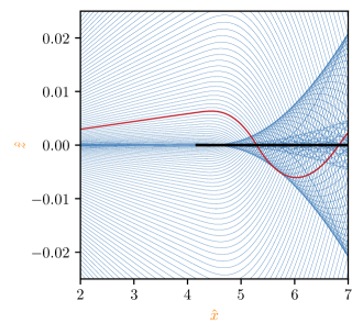
Figure 11: Region around the equator with unclipped geodesics illustrating the oscillating behavior of the solution when extended beyond the touching point at the disk. One arbitrary geodesic has been highlighted. Note that the plot does not have equal coordinate scales and shows a region farther away from the black hole than other plots. Moreover, a denser set of geodesics has been used for this plot and the geodesics were mirrored with respect to the ${\color[rgb]{1,.5,0}{\hat{x}}}$ axis to fill the region with ${\color[rgb]{1,.5,0}{\hat{z}}}<0$.

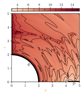
Figure 12: Precision of the numerical solution as demonstrated by $\log\left|{\color[rgb]{0,0,1}{\pi}}/\left[{\color[rgb]{0,0,1}{\pi}}-\left({\color[rgb]{0,0,1}{\alpha}}+\mkern 2.0mu\overline{\mkern-2.0mu{\color[rgb]{0,0,1}{\beta}}\mkern-0.7mu}\mkern 0.7mu\right)\right]\right|$. The value corresponds to the number of correct digits. The data for the figure has been made by evaluating the 2-dimensional interpolating functions representing the spin coefficients on a grid of $\approx 10^{2}$ points in each dimension, this grid was then used by matplotlib to construct the contours.

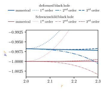
Figure 13: The value of ${\color[rgb]{0,0,1}{\mu}}$ computed by the numerical solution is compared to its analytic expansion for both the example deformation by a thin disk (thicker blue lines) and the pure Schwarzschild term (red thinner lines). The expansion, demonstrated up to the $1^{\text{st}}$, $2^{\text{nd}}$ and $3^{\text{rd}}$ orders, is displayed by dashed and dotted lines, while the numerical solution is drawn by a solid line. The values are multiplied by ${\color[rgb]{1,.5,0}{r}}$ to highlight the differences.

C.2 Numerical methods

While the disk [23] used as an example has analytic expressions for both metric functions $\zeta$ and $\psi$ available in the whole region outside the black hole, usually the function $\zeta$ is known only at the horizon and symmetry axis. Therefore, while we could have used directly the numerical value of $\zeta$ and $\psi$, we had used only their value on the horizon paired with the derivatives of $\psi$ outside to numerically integrate the function using the Einstein equations (60b) and (60c).

To solve the set of differential equations and initial data from Sec. C.1 given at their singular point (the horizon), we used Mathematica’s sixth-order ExplicitRungeKutta method with the DoubleStep option, which provided the numerical solution with precision $\approx 10^{-9}$. Because the implemented step-size control led to a very small step size near the horizon, we had to use multiple precision arithmetic available in Mathematica.

For interpolation, we wanted to use the discrete cosine transform (DCT). However, we encountered issues caused by the Gibbs effect. Hence, we decided to use the same built-in Mathematica’s interpolation as was used by the radial solution, but the number of the used geodesics had to be increased. While in Fig. 2 only a few geodesics were shown to illustrate the problem, for the numerical solution, 200 geodesics were computed, the starting angles for the geodesics were chosen to be at the Chebyshev nodes of the first kind scaled to the interval $(0,\frac{\kern 0.27995pt\uppi\kern 0.27995pt}{2})$, [32].

One notable difficulty is that the Hamilton equations may become invalid when the geodesic touches or comes very close to the disk. This issue is illustrated in Fig. 11. Each geodesic was clipped at the point where it touches the disk to prevent overlapping coordinates, which could cause problems. The crossing of geodesics at the disk is expected and has been discussed in [15].

C.3 Numerical errors

To check the validity and precision of the numerical solution, we verified selected identities that should be satisfied by the computed quantities. One particular example is shown in Fig. 12.

Moreover, we also checked that the numerical solution and the series yield the same results near the horizon where the series corresponds to the full solution well. In Fig. 13, we illustrated the difference for one particular NP scalar.

Appendix D Model Weyl metric: black hole and disk

The Morgan–Morgan class of disks comprise of disks with mass ${\color[rgb]{0.5,0.5,0}{\mathcal{M}}}$ and Newtonian density profile

$$\sigma^{(n)}_{\text{MM}}({\color[rgb]{1,.5,0}{\varrho}}\leq{\color[rgb]{0.5,0.5,0}{b}}) =\frac{(2n+1){\color[rgb]{0.5,0.5,0}{\mathcal{M}}}}{2\kern 0.39993pt\uppi\kern 0.39993pt{\color[rgb]{0.5,0.5,0}{b}}^{2}}\left(1-\frac{{\color[rgb]{1,.5,0}{\varrho}}^{2}}{{\color[rgb]{0.5,0.5,0}{b}}^{2}}\right)^{n-\frac{1}{2}}\,,$$ (119)

$$\sigma^{(n)}_{\text{MM}}({\color[rgb]{1,.5,0}{\varrho}}\geq{\color[rgb]{0.5,0.5,0}{b}}) =0\,.$$

The Newtonian potential $\psi$ was found in [34].

By performing the Kelvin transformation, we get inverted Morgan–Morgan disks—holey disks with an inner rim at ${\color[rgb]{1,.5,0}{\varrho}}={\color[rgb]{0.5,0.5,0}{b}}$ and density distributions as

$$\sigma_{\text{iMM}}^{(n)}({\color[rgb]{1,.5,0}{\varrho}}\leq{\color[rgb]{0.5,0.5,0}{b}}) =0\,,$$

$$\sigma_{\text{iMM}}^{(n)}({\color[rgb]{1,.5,0}{\varrho}}\geq{\color[rgb]{0.5,0.5,0}{b}}) =\frac{2^{2n}(n!)^{2}{\color[rgb]{0.5,0.5,0}{\mathcal{M}}}\,{\color[rgb]{0.5,0.5,0}{b}}}{(2n)!\,\kern 0.39993pt\uppi\kern 0.39993pt^{2}{\color[rgb]{1,.5,0}{\varrho}}^{3}}\left(1-\frac{{\color[rgb]{0.5,0.5,0}{b}}^{2}}{{\color[rgb]{1,.5,0}{\varrho}}^{2}}\right)^{n-\frac{1}{2}}\,.$$

Such a disk can be, in Weyl coordinates, easily superposed with the Schwarzschild black hole.

The exact analytical solution for both of the metric functions has been recently provided in [23]. For the sake of simplicity, we use the simplest case $n=2$ (for $n=1$ the density has a sharp onset) as a particular example. We thus used the following expressions given in the oblate spheroidal coordinates for our numerical calculations:

$$\begin{split}\psi_{\text{d}}&=-\frac{{\color[rgb]{0.5,0.5,0}{\mathcal{M}}}}{4{\color[rgb]{0.5,0.5,0}{b}}\kern 0.39993pt\uppi\kern 0.39993pt{\color[rgb]{0.5,0.5,0}{d}}^{\frac{9}{2}}}\,\mathcal{P}^{\nu}_{1}({\color[rgb]{0,0,0}{\hat{\xi}}},{\color[rgb]{0,0,0}{\hat{\zeta}}})\operatorname{arccot}\!\left(\frac{|{\color[rgb]{0,0,0}{\hat{\xi}}}|}{\sqrt{{\color[rgb]{0.5,0.5,0}{d}}}}\right)+\frac{{\color[rgb]{0.5,0.5,0}{\mathcal{M}}}^{2}}{12{\color[rgb]{0.5,0.5,0}{b}}\kern 0.39993pt\uppi\kern 0.39993pt{\color[rgb]{0.5,0.5,0}{d}}^{4}}\mathcal{P}^{\nu}_{0}({\color[rgb]{0,0,0}{\hat{\xi}}},{\color[rgb]{0,0,0}{\hat{\zeta}}})\,,\end{split}$$ (120a)

$$\begin{split}\zeta_{\text{d}}&=\frac{{\color[rgb]{0.5,0.5,0}{\mathcal{M}}}^{2}}{1440{\color[rgb]{0.5,0.5,0}{b}}^{2}\kern 0.39993pt\uppi\kern 0.39993pt^{2}{\color[rgb]{0.5,0.5,0}{d}}^{9}}\mathcal{P}^{d}_{0}({\color[rgb]{0,0,0}{\hat{\xi}}},{\color[rgb]{0,0,0}{\hat{\zeta}}})-\frac{{\color[rgb]{0.5,0.5,0}{\mathcal{M}}}^{2}}{48{\color[rgb]{0.5,0.5,0}{b}}^{2}\kern 0.39993pt\uppi\kern 0.39993pt^{2}{\color[rgb]{0.5,0.5,0}{d}}^{\frac{19}{2}}}\mathcal{P}^{d}_{1}({\color[rgb]{0,0,0}{\hat{\xi}}},{\color[rgb]{0,0,0}{\hat{\zeta}}})\operatorname{arccot}\!\left(\frac{|{\color[rgb]{0,0,0}{\hat{\xi}}}|}{\sqrt{{\color[rgb]{0.5,0.5,0}{d}}}}\right)+\frac{{\color[rgb]{0.5,0.5,0}{\mathcal{M}}}^{2}}{32{\color[rgb]{0.5,0.5,0}{b}}^{2}\kern 0.39993pt\uppi\kern 0.39993pt^{2}{\color[rgb]{0.5,0.5,0}{d}}^{10}}\mathcal{P}^{d}_{2}({\color[rgb]{0,0,0}{\hat{\xi}}},{\color[rgb]{0,0,0}{\hat{\zeta}}})\operatorname{arccot}^{2}\!\left(\frac{|{\color[rgb]{0,0,0}{\hat{\xi}}}|}{\sqrt{{\color[rgb]{0.5,0.5,0}{d}}}}\right),\end{split}$$ (120b)

$$\begin{split}\zeta_{\text{i}}&=\frac{2\left({\color[rgb]{0.5,0.5,0}{b}}^{2}+{\color[rgb]{0.5,0.5,0}{M}}^{2}\right)^{2}{\color[rgb]{0.5,0.5,0}{\mathcal{M}}}}{{\color[rgb]{0.5,0.5,0}{M}}^{5}\kern 0.39993pt\uppi\kern 0.39993pt}\,\Bigl{[}\arctan\!\left(-{\color[rgb]{0.5,0.5,0}{M}}{\color[rgb]{0,0,0}{\hat{\zeta}}}+{\color[rgb]{0.5,0.5,0}{b}}{\color[rgb]{0,0,0}{\hat{\xi}}}\,,l_{\text{p}}({\color[rgb]{0,0,0}{\hat{\xi}}},{\color[rgb]{0,0,0}{\hat{\zeta}}})\right)+\arctan\!\left({\color[rgb]{0.5,0.5,0}{M}}{\color[rgb]{0,0,0}{\hat{\zeta}}}+{\color[rgb]{0.5,0.5,0}{b}}{\color[rgb]{0,0,0}{\hat{\xi}}}\,,l_{\text{m}}({\color[rgb]{0,0,0}{\hat{\xi}}},{\color[rgb]{0,0,0}{\hat{\zeta}}})\right)\Bigr{]}\\ &\qquad+\frac{{\color[rgb]{0.5,0.5,0}{\mathcal{M}}}}{24{\color[rgb]{0.5,0.5,0}{b}}{\color[rgb]{0.5,0.5,0}{M}}^{5}{\color[rgb]{0.5,0.5,0}{d}}^{\frac{9}{2}}}\Biggl{[}\left(-2{\color[rgb]{0.5,0.5,0}{M}}{\color[rgb]{0.5,0.5,0}{d}}\,\mathcal{P}^{i}_{1}({\color[rgb]{0,0,0}{\hat{\xi}}},{\color[rgb]{0,0,0}{\hat{\zeta}}})+\Bigl{(}\mathcal{P}^{i}_{2}({\color[rgb]{0,0,0}{\hat{\xi}}},{\color[rgb]{0,0,0}{\hat{\zeta}}})+\mathcal{P}^{i}_{3}({\color[rgb]{0,0,0}{\hat{\xi}}},{\color[rgb]{0,0,0}{\hat{\zeta}}})\Bigr{)}\,\operatorname{arccot}\!\left(\frac{|{\color[rgb]{0,0,0}{\hat{\xi}}}|}{{\color[rgb]{0.5,0.5,0}{d}}}\right)\!\right)l_{\text{p}}({\color[rgb]{0,0,0}{\hat{\xi}}},{\color[rgb]{0,0,0}{\hat{\zeta}}})\\ &\phantom{\qquad+\frac{{\color[rgb]{0.5,0.5,0}{\mathcal{M}}}}{24{\color[rgb]{0.5,0.5,0}{b}}{\color[rgb]{0.5,0.5,0}{M}}^{5}{\color[rgb]{0.5,0.5,0}{d}}^{\frac{9}{2}}}\Bigl{[}}+\left(2{\color[rgb]{0.5,0.5,0}{M}}{\color[rgb]{0.5,0.5,0}{d}}\,\mathcal{P}^{i}_{1}(-{\color[rgb]{0,0,0}{\hat{\xi}}},{\color[rgb]{0,0,0}{\hat{\zeta}}})+\Bigl{(}\mathcal{P}^{i}_{2}({\color[rgb]{0,0,0}{\hat{\xi}}},{\color[rgb]{0,0,0}{\hat{\zeta}}})-\mathcal{P}^{i}_{3}({\color[rgb]{0,0,0}{\hat{\xi}}},{\color[rgb]{0,0,0}{\hat{\zeta}}})\Bigr{)}\,\operatorname{arccot}\!\left(\frac{|{\color[rgb]{0,0,0}{\hat{\xi}}}|}{{\color[rgb]{0.5,0.5,0}{d}}}\right)\!\right)l_{\text{m}}({\color[rgb]{0,0,0}{\hat{\xi}}},{\color[rgb]{0,0,0}{\hat{\zeta}}})\Biggr{]}\,,\end{split}$$ (120c)

where $\mathcal{P}^{\bullet}_{\bullet}({\color[rgb]{0,0,0}{\hat{\xi}}},{\color[rgb]{0,0,0}{\hat{\zeta}}})$ are polynomials in their arguments whose particular form is postponed to Sec. D.1. The function $\arctan(x,y)$ with two arguments gives the proper angle $\phi$ taking into account the quadrants in which a point $(x,y)$ lies; i.e. such that $x=\cos\phi$ and $y=\sin\phi$. The distance ${\color[rgb]{0.5,0.5,0}{d}}=1+{\color[rgb]{0,0,0}{\hat{\zeta}}}^{2}-{\color[rgb]{0,0,0}{\hat{\xi}}}^{2}=({\color[rgb]{1,.5,0}{\varrho}}^{2}+{\color[rgb]{1,.5,0}{z}}^{2})/{\color[rgb]{0.5,0.5,0}{b}}^{2}$ and the functions $l_{\text{p}}({\color[rgb]{0,0,0}{\hat{\xi}}},{\color[rgb]{0,0,0}{\hat{\zeta}}})$ and $l_{\text{m}}({\color[rgb]{0,0,0}{\hat{\xi}}},{\color[rgb]{0,0,0}{\hat{\zeta}}})$ are identical to $l_{\text{p}}$ and $l_{\text{m}}$ from (52) but expressed in the oblate spheroidal coordinates:

$$\begin{aligned} l_{\text{p}}&=\sqrt{\left({\color[rgb]{0.5,0.5,0}{d}}\,{\color[rgb]{0,0,0}{\hat{\xi}}}\,{\color[rgb]{0,0,0}{\hat{\zeta}}}+{\color[rgb]{0.5,0.5,0}{M}}\right)^{2}+{\color[rgb]{0.5,0.5,0}{d}}^{2}\left(1-{\color[rgb]{0,0,0}{\hat{\xi}}}^{2}\right)\left(1+{\color[rgb]{0,0,0}{\hat{\zeta}}}^{2}\right)}\,,\\ l_{\text{m}}&=\sqrt{\left({\color[rgb]{0.5,0.5,0}{d}}\,{\color[rgb]{0,0,0}{\hat{\xi}}}\,{\color[rgb]{0,0,0}{\hat{\zeta}}}-{\color[rgb]{0.5,0.5,0}{M}}\right)^{2}+{\color[rgb]{0.5,0.5,0}{d}}^{2}\left(1-{\color[rgb]{0,0,0}{\hat{\xi}}}^{2}\right)\left(1+{\color[rgb]{0,0,0}{\hat{\zeta}}}^{2}\right)}\,.\end{aligned}$$

The oblate spheroidal coordinates ${\color[rgb]{0,0,0}{\hat{\zeta}}}\in[0,\infty)$ and ${\color[rgb]{0,0,0}{\hat{\xi}}}\in[-1,+1]$, in which the expressions related to the disk take the simplest form, are defined by

$${\color[rgb]{1,.5,0}{\varrho}}^{2} ={\color[rgb]{0.5,0.5,0}{b}}^{2}\left(1+{\color[rgb]{0,0,0}{\hat{\zeta}}}^{2}\right)\!\left(1-{\color[rgb]{0,0,0}{\hat{\xi}}}^{2}\right), {\color[rgb]{1,.5,0}{z}} ={\color[rgb]{0.5,0.5,0}{b}}\,{\color[rgb]{0,0,0}{\hat{\zeta}}}\,{\color[rgb]{0,0,0}{\hat{\xi}}}\,.$$

The inverse relations read

$${\color[rgb]{0,0,0}{\hat{\zeta}}} =\frac{\sqrt{2}\left|{\color[rgb]{1,.5,0}{z}}\right|}{\sqrt{\sqrt{u^{2}+4{\color[rgb]{0.5,0.5,0}{b}}^{2}{\color[rgb]{1,.5,0}{z}}^{2}}-u}}\,, {\color[rgb]{0,0,0}{\hat{\xi}}} =\frac{{\color[rgb]{1,.5,0}{z}}}{{\color[rgb]{0.5,0.5,0}{b}}{\color[rgb]{0,0,0}{\hat{\zeta}}}}\,,$$

where we set $u={\color[rgb]{1,.5,0}{\varrho}}^{2}-{\color[rgb]{0.5,0.5,0}{b}}^{2}+{\color[rgb]{1,.5,0}{z}}^{2}$.

The final solution of EFEs is given by

$$\begin{aligned} \psi&=\psi_{\text{S}}+\psi_{\text{d}}\,,\\ \zeta&=\zeta_{\text{S}}+\zeta_{\text{i}}+\zeta_{\text{d}}\,,\end{aligned}$$

where $\psi_{\text{S}}$ is the Schwarzschild Newtonian potential and $\psi_{\text{d}}$ is the Newtonian potential of the disk itself. Due to the non-linearity of EFEs, the $\zeta$ has three different contributions: from the Schwarzschild black hole solely $\zeta_{\text{S}}$, from the disk solely $\zeta_{\text{d}}$ and the interaction term $\zeta_{\text{i}}$.

If one adheres to the counter-rotating dust streams interpretation of a static disk, one has to ensure that the speed of individual particles is subluminal (i.e. $0<v^{2}<1$). The individual dust particles should follow a time-like geodesics of constant radius in the equatorial plane. Then their speed $v$ can be calculated as

$$v^{2} =\frac{{\color[rgb]{1,.5,0}{\varrho}}\,\psi_{,{\color[rgb]{1,.5,0}{\varrho}}}}{1-{\color[rgb]{1,.5,0}{\varrho}}\,\psi_{,{\color[rgb]{1,.5,0}{\varrho}}}}\,,$$

in Weyl coordinates.

This gives us a constrain on the admissible parameter space ${\color[rgb]{0.5,0.5,0}{M}}$, ${\color[rgb]{0.5,0.5,0}{\mathcal{M}}}$ and ${\color[rgb]{0.5,0.5,0}{b}}$. For our particular choice of disks, we have

$$0<\frac{8{\color[rgb]{1,.5,0}{\varrho}}^{5}\sqrt{{\color[rgb]{0.5,0.5,0}{M}}^{2}+{\color[rgb]{1,.5,0}{\varrho}}^{2}}}{8{\color[rgb]{1,.5,0}{\varrho}}^{5}\left(\sqrt{{\color[rgb]{0.5,0.5,0}{M}}^{2}+{\color[rgb]{1,.5,0}{\varrho}}^{2}}-{\color[rgb]{0.5,0.5,0}{M}}\right)-p{\color[rgb]{0.5,0.5,0}{\mathcal{M}}}\sqrt{{\color[rgb]{0.5,0.5,0}{M}}^{2}+{\color[rgb]{1,.5,0}{\varrho}}^{2}}}-1<1\,,$$ (121)

where

$$p=15{\color[rgb]{0.5,0.5,0}{b}}^{4}-24{\color[rgb]{0.5,0.5,0}{b}}^{2}{\color[rgb]{1,.5,0}{\varrho}}^{2}+8{\color[rgb]{1,.5,0}{\varrho}}^{4}\,,$$ (122)

which has to hold for all ${\color[rgb]{1,.5,0}{\varrho}}>{\color[rgb]{0.5,0.5,0}{b}}$.

In other words, the inner rim of the disc must be positioned above the equatorial photon orbit (whose radius is $3{\color[rgb]{0.5,0.5,0}{M}}$ for Schwarzschild). The radius of this orbit is influenced by the presence of the gravitating disk itself.

In principle, since the orbits between the photon orbit and the innermost stable circular orbit (ISCO), [35], are unstable, in an astrophysically relevant system, the inner rim of the disk should be set above the ISCO. As we want to make the gravitational influence of the disk as prominent as possible, we push the parameters to the extreme. A detailed discussion of the stability of these discs can be found in [36].

D.1 The disk polynomials

The explicit form of the polynomials appearing in the disk solution from [23] is as follows

$$\begin{split}\mathcal{P}^{\nu}_{0}({\color[rgb]{0,0,0}{\hat{\xi}}},{\color[rgb]{0,0,0}{\hat{\zeta}}})&=\left[40{\color[rgb]{0,0,0}{\hat{\zeta}}}^{6}+8{\color[rgb]{0,0,0}{\hat{\zeta}}}^{4}\left({\color[rgb]{0,0,0}{\hat{\xi}}}^{2}+2\right)+{\color[rgb]{0,0,0}{\hat{\zeta}}}^{2}\left(39{\color[rgb]{0,0,0}{\hat{\xi}}}^{4}-6{\color[rgb]{0,0,0}{\hat{\xi}}}^{2}-33\right)+9\left({\color[rgb]{0,0,0}{\hat{\xi}}}^{2}-1\right)^{2}\left(2{\color[rgb]{0,0,0}{\hat{\xi}}}^{2}-1\right)\right]\left|{\color[rgb]{0,0,0}{\hat{\xi}}}\right|,\end{split}$$

$$\begin{split}\mathcal{P}^{\nu}_{1}({\color[rgb]{0,0,0}{\hat{\xi}}},{\color[rgb]{0,0,0}{\hat{\zeta}}})&=-8\left({\color[rgb]{0,0,0}{\hat{\zeta}}}^{2}+3\right){\color[rgb]{0,0,0}{\hat{\xi}}}^{6}+\left(35{\color[rgb]{0,0,0}{\hat{\zeta}}}^{4}+54{\color[rgb]{0,0,0}{\hat{\zeta}}}^{2}+27\right){\color[rgb]{0,0,0}{\hat{\xi}}}^{4}-2\left({\color[rgb]{0,0,0}{\hat{\zeta}}}^{2}+1\right)\left(4{\color[rgb]{0,0,0}{\hat{\zeta}}}^{4}+23{\color[rgb]{0,0,0}{\hat{\zeta}}}^{2}+7\right){\color[rgb]{0,0,0}{\hat{\xi}}}^{2}\\ &\qquad+\left({\color[rgb]{0,0,0}{\hat{\zeta}}}^{2}+1\right)^{2}\left(8{\color[rgb]{0,0,0}{\hat{\zeta}}}^{4}+8{\color[rgb]{0,0,0}{\hat{\zeta}}}^{2}+3\right)+8{\color[rgb]{0,0,0}{\hat{\xi}}}^{8}.\end{split}$$

$$\begin{split}\mathcal{P}^{d}_{0}({\color[rgb]{0,0,0}{\hat{\xi}}},{\color[rgb]{0,0,0}{\hat{\zeta}}})&=\left({\color[rgb]{0,0,0}{\hat{\xi}}}^{2}-1\right)\Bigl{[}320{\color[rgb]{0,0,0}{\hat{\zeta}}}^{14}\left(201{\color[rgb]{0,0,0}{\hat{\xi}}}^{2}-32\right)+320{\color[rgb]{0,0,0}{\hat{\zeta}}}^{12}\left(235{\color[rgb]{0,0,0}{\hat{\xi}}}^{4}+484{\color[rgb]{0,0,0}{\hat{\xi}}}^{2}-160\right)\\ &\qquad{}+240{\color[rgb]{0,0,0}{\hat{\zeta}}}^{10}\left(1287{\color[rgb]{0,0,0}{\hat{\xi}}}^{6}-698{\color[rgb]{0,0,0}{\hat{\xi}}}^{4}+679{\color[rgb]{0,0,0}{\hat{\xi}}}^{2}-448\right)\\ &\qquad+4{\color[rgb]{0,0,0}{\hat{\zeta}}}^{8}\left(40449{\color[rgb]{0,0,0}{\hat{\xi}}}^{8}+100729{\color[rgb]{0,0,0}{\hat{\xi}}}^{6}-153381{\color[rgb]{0,0,0}{\hat{\xi}}}^{4}+61179{\color[rgb]{0,0,0}{\hat{\xi}}}^{2}-30976\right)\\ &\qquad+{\color[rgb]{0,0,0}{\hat{\zeta}}}^{6}\left({\color[rgb]{0,0,0}{\hat{\xi}}}-1\right)\left({\color[rgb]{0,0,0}{\hat{\xi}}}+1\right)\left(228521{\color[rgb]{0,0,0}{\hat{\xi}}}^{8}-9179{\color[rgb]{0,0,0}{\hat{\xi}}}^{6}+317611{\color[rgb]{0,0,0}{\hat{\xi}}}^{4}-262969{\color[rgb]{0,0,0}{\hat{\xi}}}^{2}+86016\right)\\ &\qquad+3{\color[rgb]{0,0,0}{\hat{\zeta}}}^{4}\left({\color[rgb]{0,0,0}{\hat{\xi}}}^{2}-1\right)^{2}\left(12192{\color[rgb]{0,0,0}{\hat{\xi}}}^{8}+84557{\color[rgb]{0,0,0}{\hat{\xi}}}^{6}-12478{\color[rgb]{0,0,0}{\hat{\xi}}}^{4}+54017{\color[rgb]{0,0,0}{\hat{\xi}}}^{2}-12288\right)\\ &\qquad+9{\color[rgb]{0,0,0}{\hat{\zeta}}}^{2}\left({\color[rgb]{0,0,0}{\hat{\xi}}}^{2}-1\right)^{3}\left(2004{\color[rgb]{0,0,0}{\hat{\xi}}}^{8}+2364{\color[rgb]{0,0,0}{\hat{\xi}}}^{6}+8059{\color[rgb]{0,0,0}{\hat{\xi}}}^{4}-4451{\color[rgb]{0,0,0}{\hat{\xi}}}^{2}+1024\right)\\ &\qquad-\left({\color[rgb]{0,0,0}{\hat{\xi}}}^{2}-1\right)^{4}\left(304{\color[rgb]{0,0,0}{\hat{\xi}}}^{8}-6436{\color[rgb]{0,0,0}{\hat{\xi}}}^{6}+7584{\color[rgb]{0,0,0}{\hat{\xi}}}^{4}-4501{\color[rgb]{0,0,0}{\hat{\xi}}}^{2}+1024\right)\Bigr{]}\,,\end{split}$$

$$\begin{split}\mathcal{P}^{d}_{1}({\color[rgb]{0,0,0}{\hat{\xi}}},{\color[rgb]{0,0,0}{\hat{\zeta}}})&=\left({\color[rgb]{0,0,0}{\hat{\xi}}}^{2}-1\right)\Bigl{[}832{\color[rgb]{0,0,0}{\hat{\zeta}}}^{16}+64{\color[rgb]{0,0,0}{\hat{\zeta}}}^{14}\left(73{\color[rgb]{0,0,0}{\hat{\xi}}}^{2}+33\right)+16{\color[rgb]{0,0,0}{\hat{\zeta}}}^{12}\left(649{\color[rgb]{0,0,0}{\hat{\xi}}}^{4}+358{\color[rgb]{0,0,0}{\hat{\xi}}}^{2}-15\right)\\ &\qquad+4{\color[rgb]{0,0,0}{\hat{\zeta}}}^{10}\left(4313{\color[rgb]{0,0,0}{\hat{\xi}}}^{6}+1917{\color[rgb]{0,0,0}{\hat{\xi}}}^{4}-1157{\color[rgb]{0,0,0}{\hat{\xi}}}^{2}-1393\right)+5{\color[rgb]{0,0,0}{\hat{\zeta}}}^{8}\left(2797{\color[rgb]{0,0,0}{\hat{\xi}}}^{8}+2632{\color[rgb]{0,0,0}{\hat{\xi}}}^{6}-3046{\color[rgb]{0,0,0}{\hat{\xi}}}^{4}-64{\color[rgb]{0,0,0}{\hat{\xi}}}^{2}-1359\right)\\ &\qquad+2{\color[rgb]{0,0,0}{\hat{\zeta}}}^{6}\left({\color[rgb]{0,0,0}{\hat{\xi}}}-1\right)\left({\color[rgb]{0,0,0}{\hat{\xi}}}+1\right)\left(4789{\color[rgb]{0,0,0}{\hat{\xi}}}^{8}+6849{\color[rgb]{0,0,0}{\hat{\xi}}}^{6}+3889{\color[rgb]{0,0,0}{\hat{\xi}}}^{4}-5321{\color[rgb]{0,0,0}{\hat{\xi}}}^{2}+1794\right)\\ &\qquad+2{\color[rgb]{0,0,0}{\hat{\zeta}}}^{4}\left({\color[rgb]{0,0,0}{\hat{\xi}}}^{2}-1\right)^{2}\left(1200{\color[rgb]{0,0,0}{\hat{\xi}}}^{8}+5395{\color[rgb]{0,0,0}{\hat{\xi}}}^{6}+2331{\color[rgb]{0,0,0}{\hat{\xi}}}^{4}+4203{\color[rgb]{0,0,0}{\hat{\xi}}}^{2}-529\right)\\ &\qquad+6{\color[rgb]{0,0,0}{\hat{\zeta}}}^{2}\left({\color[rgb]{0,0,0}{\hat{\xi}}}^{2}-1\right)^{3}\left(72{\color[rgb]{0,0,0}{\hat{\xi}}}^{8}+328{\color[rgb]{0,0,0}{\hat{\xi}}}^{6}+653{\color[rgb]{0,0,0}{\hat{\xi}}}^{4}-193{\color[rgb]{0,0,0}{\hat{\xi}}}^{2}+40\right)+3\left({\color[rgb]{0,0,0}{\hat{\xi}}}^{2}-1\right)^{4}\left(80{\color[rgb]{0,0,0}{\hat{\xi}}}^{6}-64{\color[rgb]{0,0,0}{\hat{\xi}}}^{4}+38{\color[rgb]{0,0,0}{\hat{\xi}}}^{2}-9\right)\Bigr{]}\left|{\color[rgb]{0,0,0}{\hat{\xi}}}\right|,\end{split}$$

$$\begin{split}\mathcal{P}^{d}_{2}({\color[rgb]{0,0,0}{\hat{\xi}}},{\color[rgb]{0,0,0}{\hat{\zeta}}})&=\left({\color[rgb]{0,0,0}{\hat{\zeta}}}^{2}+1\right)\left({\color[rgb]{0,0,0}{\hat{\xi}}}^{2}-1\right)\Bigl{[}64{\color[rgb]{0,0,0}{\hat{\zeta}}}^{16}+64{\color[rgb]{0,0,0}{\hat{\zeta}}}^{14}\left(7{\color[rgb]{0,0,0}{\hat{\xi}}}^{2}+5\right)+16{\color[rgb]{0,0,0}{\hat{\zeta}}}^{12}\left(157{\color[rgb]{0,0,0}{\hat{\xi}}}^{4}-18{\color[rgb]{0,0,0}{\hat{\xi}}}^{2}+45\right)\\ &\qquad+4{\color[rgb]{0,0,0}{\hat{\zeta}}}^{10}\left(949{\color[rgb]{0,0,0}{\hat{\xi}}}^{6}+785{\color[rgb]{0,0,0}{\hat{\xi}}}^{4}-1025{\color[rgb]{0,0,0}{\hat{\xi}}}^{2}+251\right)\\ &\qquad+5{\color[rgb]{0,0,0}{\hat{\zeta}}}^{8}\left(1241{\color[rgb]{0,0,0}{\hat{\xi}}}^{8}-560{\color[rgb]{0,0,0}{\hat{\xi}}}^{6}+730{\color[rgb]{0,0,0}{\hat{\xi}}}^{4}-1288{\color[rgb]{0,0,0}{\hat{\xi}}}^{2}+197\right)\\ &\qquad+4{\color[rgb]{0,0,0}{\hat{\zeta}}}^{6}\left({\color[rgb]{0,0,0}{\hat{\xi}}}-1\right)\left({\color[rgb]{0,0,0}{\hat{\xi}}}+1\right)\left(949{\color[rgb]{0,0,0}{\hat{\xi}}}^{8}+1649{\color[rgb]{0,0,0}{\hat{\xi}}}^{6}-1356{\color[rgb]{0,0,0}{\hat{\xi}}}^{4}+929{\color[rgb]{0,0,0}{\hat{\xi}}}^{2}-171\right)\\ &\qquad+2{\color[rgb]{0,0,0}{\hat{\zeta}}}^{4}\left({\color[rgb]{0,0,0}{\hat{\xi}}}^{2}-1\right)^{2}\left(1256{\color[rgb]{0,0,0}{\hat{\xi}}}^{8}+942{\color[rgb]{0,0,0}{\hat{\xi}}}^{6}+2453{\color[rgb]{0,0,0}{\hat{\xi}}}^{4}-606{\color[rgb]{0,0,0}{\hat{\xi}}}^{2}+155\right)\\ &\qquad+4{\color[rgb]{0,0,0}{\hat{\zeta}}}^{2}(2{\color[rgb]{0,0,0}{\hat{\xi}}}-1)(2{\color[rgb]{0,0,0}{\hat{\xi}}}+1)\left({\color[rgb]{0,0,0}{\hat{\xi}}}^{2}-1\right)^{3}\left({\color[rgb]{0,0,0}{\hat{\xi}}}^{2}+4\right)\left(28{\color[rgb]{0,0,0}{\hat{\xi}}}^{4}-3{\color[rgb]{0,0,0}{\hat{\xi}}}^{2}+5\right)\\ &\qquad+\left({\color[rgb]{0,0,0}{\hat{\xi}}}^{2}-1\right)^{4}\left(64{\color[rgb]{0,0,0}{\hat{\xi}}}^{8}-64{\color[rgb]{0,0,0}{\hat{\xi}}}^{6}+80{\color[rgb]{0,0,0}{\hat{\xi}}}^{4}-44{\color[rgb]{0,0,0}{\hat{\xi}}}^{2}+9\right)\Bigr{]}\,,\end{split}$$

$$\begin{split}\mathcal{P}^{i}_{1}({\color[rgb]{0,0,0}{\hat{\xi}}},{\color[rgb]{0,0,0}{\hat{\zeta}}})&=24{\color[rgb]{0.5,0.5,0}{b}}^{3}{\color[rgb]{0,0,0}{\hat{\zeta}}}\left({\color[rgb]{0,0,0}{\hat{\zeta}}}^{2}-{\color[rgb]{0,0,0}{\hat{\xi}}}^{2}+1\right)^{3}-12{\color[rgb]{0.5,0.5,0}{b}}^{2}{\color[rgb]{0.5,0.5,0}{M}}{\color[rgb]{0,0,0}{\hat{\xi}}}\left({\color[rgb]{0,0,0}{\hat{\zeta}}}^{2}-{\color[rgb]{0,0,0}{\hat{\xi}}}^{2}+1\right)^{2}\left(2{\color[rgb]{0,0,0}{\hat{\zeta}}}^{2}+{\color[rgb]{0,0,0}{\hat{\xi}}}^{2}-1\right)\\ &\qquad+4{\color[rgb]{0.5,0.5,0}{b}}{\color[rgb]{0,0,0}{\hat{\zeta}}}{\color[rgb]{0.5,0.5,0}{M}}^{2}\left[10{\color[rgb]{0,0,0}{\hat{\zeta}}}^{6}+{\color[rgb]{0,0,0}{\hat{\zeta}}}^{4}\left(26-20{\color[rgb]{0,0,0}{\hat{\xi}}}^{2}\right)+{\color[rgb]{0,0,0}{\hat{\zeta}}}^{2}\left(25{\color[rgb]{0,0,0}{\hat{\xi}}}^{4}-47{\color[rgb]{0,0,0}{\hat{\xi}}}^{2}+22\right)-3\left({\color[rgb]{0,0,0}{\hat{\xi}}}^{2}-1\right)^{2}\left(5{\color[rgb]{0,0,0}{\hat{\xi}}}^{2}-2\right)\right]\\ &\qquad-{\color[rgb]{0.5,0.5,0}{M}}^{3}{\color[rgb]{0,0,0}{\hat{\xi}}}\left[40{\color[rgb]{0,0,0}{\hat{\zeta}}}^{6}+8{\color[rgb]{0,0,0}{\hat{\zeta}}}^{4}\left({\color[rgb]{0,0,0}{\hat{\xi}}}^{2}+2\right)+{\color[rgb]{0,0,0}{\hat{\zeta}}}^{2}\left(39{\color[rgb]{0,0,0}{\hat{\xi}}}^{4}-6{\color[rgb]{0,0,0}{\hat{\xi}}}^{2}-33\right)+9\left({\color[rgb]{0,0,0}{\hat{\xi}}}^{2}-1\right)^{2}\left(2{\color[rgb]{0,0,0}{\hat{\xi}}}^{2}-1\right)\right],\end{split}$$

$$\begin{split}\mathcal{P}^{i}_{2}({\color[rgb]{0,0,0}{\hat{\xi}}},{\color[rgb]{0,0,0}{\hat{\zeta}}})&=-6\,\Bigl{[}8{\color[rgb]{0.5,0.5,0}{b}}^{4}\left({\color[rgb]{0,0,0}{\hat{\zeta}}}^{2}-{\color[rgb]{0,0,0}{\hat{\xi}}}^{2}+1\right)^{4}+4{\color[rgb]{0.5,0.5,0}{b}}^{2}{\color[rgb]{0.5,0.5,0}{M}}^{2}\left({\color[rgb]{0,0,0}{\hat{\zeta}}}^{2}-{\color[rgb]{0,0,0}{\hat{\xi}}}^{2}+1\right)^{2}\left(4{\color[rgb]{0,0,0}{\hat{\zeta}}}^{4}+{\color[rgb]{0,0,0}{\hat{\zeta}}}^{2}\left(7-5{\color[rgb]{0,0,0}{\hat{\xi}}}^{2}\right)+4{\color[rgb]{0,0,0}{\hat{\xi}}}^{4}-7{\color[rgb]{0,0,0}{\hat{\xi}}}^{2}+3\right)\\ &\qquad+{\color[rgb]{0.5,0.5,0}{M}}^{4}\Bigl{(}8{\color[rgb]{0,0,0}{\hat{\zeta}}}^{8}-8{\color[rgb]{0,0,0}{\hat{\zeta}}}^{6}\left({\color[rgb]{0,0,0}{\hat{\xi}}}^{2}-3\right)+{\color[rgb]{0,0,0}{\hat{\zeta}}}^{4}\left(35{\color[rgb]{0,0,0}{\hat{\xi}}}^{4}-54{\color[rgb]{0,0,0}{\hat{\xi}}}^{2}+27\right)+{\color[rgb]{0,0,0}{\hat{\zeta}}}^{2}\left(-8{\color[rgb]{0,0,0}{\hat{\xi}}}^{6}+54{\color[rgb]{0,0,0}{\hat{\xi}}}^{4}-60{\color[rgb]{0,0,0}{\hat{\xi}}}^{2}+14\right)\\ &\qquad+\left({\color[rgb]{0,0,0}{\hat{\xi}}}^{2}-1\right)^{2}\left(8{\color[rgb]{0,0,0}{\hat{\xi}}}^{4}-8{\color[rgb]{0,0,0}{\hat{\xi}}}^{2}+3\right)\Bigr{)}\Bigr{]}\,,\end{split}$$

$$\begin{split}\mathcal{P}^{i}_{3}({\color[rgb]{0,0,0}{\hat{\xi}}},{\color[rgb]{0,0,0}{\hat{\zeta}}})&=24{\color[rgb]{0.5,0.5,0}{b}}{\color[rgb]{0,0,0}{\hat{\zeta}}}{\color[rgb]{0.5,0.5,0}{M}}{\color[rgb]{0,0,0}{\hat{\xi}}}\left({\color[rgb]{0,0,0}{\hat{\zeta}}}^{2}-{\color[rgb]{0,0,0}{\hat{\xi}}}^{2}+1\right)\left[2{\color[rgb]{0.5,0.5,0}{b}}^{2}\left({\color[rgb]{0,0,0}{\hat{\zeta}}}^{2}-{\color[rgb]{0,0,0}{\hat{\xi}}}^{2}+1\right)^{2}+{\color[rgb]{0.5,0.5,0}{M}}^{2}\left(4{\color[rgb]{0,0,0}{\hat{\zeta}}}^{4}+{\color[rgb]{0,0,0}{\hat{\zeta}}}^{2}\left(5-3{\color[rgb]{0,0,0}{\hat{\xi}}}^{2}\right)+4{\color[rgb]{0,0,0}{\hat{\xi}}}^{4}-5{\color[rgb]{0,0,0}{\hat{\xi}}}^{2}+1\right)\right].\end{split}$$

References

- Ashtekar and Krishnan [2004] A. Ashtekar and B. Krishnan, Isolated and Dynamical Horizons and Their Applications, Living Reviews in Relativity 7, 10 (2004).
- Ashtekar et al. [2000] A. Ashtekar, S. Fairhurst, and B. Krishnan, Isolated horizons: Hamiltonian evolution and the first law, Phys. Rev. D 62, 104025 (2000).
- Ashtekar et al. [1998] A. Ashtekar, J. Baez, A. Corichi, and K. Krasnov, Quantum Geometry and Black Hole Entropy, Phys. Rev. Lett. 80, 904 (1998).
- Hayward [1994] S. A. Hayward, General laws of black-hole dynamics, Phys. Rev. D 49, 6467 (1994).
- Ashtekar and Krishnan [2002] A. Ashtekar and B. Krishnan, Dynamical Horizons: Energy, Angular Momentum, Fluxes, and Balance Laws, Phys. Rev. Lett. 89, 261101 (2002).
- Ashtekar et al. [1999] A. Ashtekar, C. Beetle, and S. Fairhurst, Isolated horizons: a generalization of black hole mechanics, Classical and Quantum Gravity 16, L1 (1999).
- Ashtekar et al. [2000a] A. Ashtekar, C. Beetle, and S. Fairhurst, Mechanics of isolated horizons, Classical and Quantum Gravity 17, 253 (2000a).
- Ashtekar et al. [2000b] A. Ashtekar, C. Beetle, O. Dreyer, S. Fairhurst, B. Krishnan, J. Lewandowski, and J. Wiśniewski, Generic Isolated Horizons and Their Applications, Phys. Rev. Lett. 85, 3564 (2000b).
- Ashtekar et al. [2001] A. Ashtekar, C. Beetle, and J. Lewandowski, Mechanics of rotating isolated horizons, Phys. Rev. D 64, 044016 (2001).
- Ashtekar et al. [2002] A. Ashtekar, C. Beetle, and J. Lewandowski, Geometry of generic isolated horizons, Classical and Quantum Gravity 19, 1195 (2002).
- Lewandowski et al. [2002] J. Lewandowski, T. Pawlowski, and A. Ashtekar, Geometric Characterizations of the Kerr Isolated Horizon, International Journal of Modern Physics D 11, 739 (2002).
- Lewandowski and Pawlowski [2006] J. Lewandowski and T. Pawlowski, Symmetric non-expanding horizons, Classical and Quantum Gravity 23, 6031 (2006).
- Adamo and Newman [2009] T. M. Adamo and E. T. Newman, Vacuum non-expanding horizons and shear-free null geodesic congruences, Classical and Quantum Gravity 26, 235012 (2009).
- Lewandowski [2000] J. Lewandowski, Spacetimes admitting isolated horizons, Classical and Quantum Gravity 17, L53 (2000).
- Krishnan [2012] B. Krishnan, The spacetime in the neighborhood of a general isolated black hole, Classical and Quantum Gravity 29, 205006 (2012).
- Stewart [1993] J. Stewart, Advanced General Relativity, Cambridge Monographs on Mathematical Physics (Cambridge University Press, 1993).
- Scholtz et al. [2017] M. Scholtz, A. Flandera, and N. Gürlebeck, Kerr-Newman black hole in the formalism of isolated horizons, Phys. Rev. D 96, 064024 (2017).
- Kofroň [2024] D. Kofroň, Kerr black hole in the formalism of isolated horizons, Phys. Rev. D 109, 084029 (2024).
- Newman and Penrose [1962] E. Newman and R. Penrose, An Approach to Gravitational Radiation by a Method of Spin Coefficients, Journal of Mathematical Physics 3, 566 (1962).
- Poisson [2005] E. Poisson, Metric of a Tidally Distorted Nonrotating Black Hole, Phys. Rev. Lett. 94, 161103 (2005).
- Poisson and Vlasov [2010] E. Poisson and I. Vlasov, Geometry and dynamics of a tidally deformed black hole, Phys. Rev. D 81, 024029 (2010).
- Frolov and Frolov [2003] A. V. Frolov and V. P. Frolov, Black holes in a compactified spacetime, Phys. Rev. D 67, 124025 (2003).
- Kofroň et al. [2023] D. Kofroň, P. Kotlařík, and O. Semerák, Relativistic disks by Appell-ring convolutions, arXiv e-prints , arXiv:2310.16669 (2023).
- Metidieri et al. [2024] A. R. Metidieri, B. Bonga, and B. Krishnan, Tidal deformations of slowly spinning isolated horizons, Phys. Rev. D 110, 024069 (2024).
- Gürlebeck and Scholtz [2018] N. Gürlebeck and M. Scholtz, Meissner effect for axially symmetric charged black holes, Phys. Rev. D 97, 084042 (2018).
- Ashtekar et al. [2004] A. Ashtekar, J. Engle, T. Pawlowski, and C. Van Den Broeck, Multipole moments of isolated horizons, Classical and Quantum Gravity 21, 2549 (2004).
- Carroll [2019] S. M. Carroll, Spacetime and Geometry: An Introduction to General Relativity (Cambridge University Press, 2019).
- Semerák et al. [1999] O. Semerák, T. Zellerin, and M. Žáček, The structure of superposed Weyl fields, Monthly Notices of the Royal Astronomical Society 308, 691 (1999).
- Semerák et al. [2002] O. Semerák, J. Podolský, and M. Žofka, Gravitation: Following the Prague Inspiration (World Scientific, 2002).
- Lewandowski and Pawlowski [2003] J. Lewandowski and T. Pawlowski, Extremal isolated horizons: a local uniqueness theorem, Classical and Quantum Gravity 20, 587 (2003).
- Gürlebeck and Scholtz [2017] N. Gürlebeck and M. Scholtz, Meissner effect for weakly isolated horizons, Phys. Rev. D 95, 064010 (2017).
- Boyd [2001] J. Boyd, Chebyshev and Fourier Spectral Methods: Second Revised Edition, Dover Books on Mathematics (Dover Publications, 2001).
- Wang and Xiang [2012] H. Wang and S. Xiang, On the convergence rates of Legendre approximation, Mathematics of Computation 81, https://doi.org/10.1090/S0025-5718-2011-02549-4 (2012).
- Morgan and Morgan [1969] T. Morgan and L. Morgan, The Gravitational Field of a Disk, Physical Review 183, 1097 (1969).
- Misner et al. [2017] C. W. Misner, K. S. Thorne, and J. A. Wheeler, Gravitation (Princeton University Press, 2017).
- Semerák [2003] O. Semerák, Gravitating discs around a Schwarzschild black hole: III, Classical and Quantum Gravity 20, 1613 (2003).