Multidimensional Deconvolution with Profiling

Abstract

In many experimental contexts, it is necessary to statistically remove the impact of instrumental effects in order to physically interpret measurements. This task has been extensively studied in particle physics, where the deconvolution task is called unfolding. A number of recent methods have shown how to perform high-dimensional, unbinned unfolding using machine learning. However, one of the assumptions in all of these methods is that the detector response is accurately modeled in the Monte Carlo simulation. In practice, the detector response depends on a number of nuisance parameters that can be constrained with data. We propose a new algorithm called Profile OmniFold (POF), which works in a similar iterative manner as the OmniFold (OF) algorithm while being able to simultaneously profile the nuisance parameters. We illustrate the method with a Gaussian example as a proof of concept highlighting its promising capabilities.

1 Introduction

Instrumental effects distort spectra from their true values. Statistically removing these distortions is essential for comparing results across experiments and for facilitating broad, detector-independent analysis of the data. This deconvolution task (called unfolding in particle physics) is an ill-posed inverse problem, where small changes in the measured spectrum can result in large fluctuation in the reconstructed true spectrum. In practice, one observes data from the measured spectrum from experiments, and the goal is estimate the true spectrum and quantify its uncertainty. See e.g. [1, 2, 3, 4, 5] for reviews of the problem. The detailed setup will also be introduced in section 2.1.

Traditionally, unfolding has been solved in discretized setting, where measurements are binned into histograms (or are naturally represented as discrete, e.g. in images) and the reconstructed spectrum is also represented as histograms. However, this requires pre-specifying the number of bins, which itself is a tuning parameter and can vary between different experiments. Additionally, binning limits the number of observables that can be simultaneously unfolded.

A number of machine learning-based approaches have been proposed to address this problem [6, 7]. The first one to be deployed to experimental data [8, 9, 10, 11, 12, 13, 14, 15, 16, 17, 18] is OmniFold [19, 20]. Unlike traditional methods, OmniFold does not require binning and can be used to unfold observables in much higher dimensions using neural network (NN) classifiers. The algorithm is an instance of Expectation-Maximization (EM) algorithm, which iteratively reweights the simulated events to match the experimental data. The result is guaranteed to converge to the maximum likelihood estimate. However, one limitation in the OmniFold, as in all machine learning-based unfolding methods, is the assumption that the detector response is correctly modeled in simulation. In practice, this is only approximately true, with a number of nuisance parameters that can be constrained by data.

Recently, Ref. [21] introduced an unbinned unfolding method that also allows for profiling the nuisance parameters. This is achieved by using machine learning to directly maximize the log-likelihood function. While a significant step forward, this approach is limited to the case where the detector-level data are binned so that one can write down the explicit likelihood (each bin is Poisson distributed).

In this work, we propose a new algorithm, called Profile OmniFold (POF), for unbinned and profiled unfolding. Unlike Ref. [21], POF is completely unbinned at both the detector-level and pre-detector-level (‘particle level’). Additionally, POF can be seen as an extension to the original OF algorithm that iteratively reweights the simulated particle-level events but also simultaneously determines the nuisance parameters.

2 Methodology

In this section, we introduce POF, which is a modified version of the original OF algorithm. Same as the original OF, the goal of POF is to find the maximum likelihood estimate of the reweighting function that reweights generated particle-level data $q(x)$ to the truth $p(x)$. However, unlike in the original OF algorithm, POF can also take into account of the nuisance parameters in the detector modeling and simultaneously profile out these nuisance parameters. At the same time, POF retains the same benefits as OF such that it can directly work with unbinned data, utilize the power of NN classifiers, and unfold multidimensional observables or even the entire phase space simultaneously [19].

2.1 Statistical setup of the unfolding problem in the presence of nuisance parameter

In unfolding problem, we are provided pairs of Monte Carlo (MC) simulation $\{X_{i},Y_{i}\}_{i=1}^{n}\sim q(x,y)$ where $X_{i}$ denote the particle-level quantity and $Y_{i}$ denote the corresponding detector-level observation. Then given a set of observed detector-level experimental data $\{Y_{i}^{\prime}\}_{i=1}^{m}\sim p(y)$, our goal is to estimate the true particle-level density $p(x)$. The forward model for both MC simulation and experimental data are described by

$$q(y)=\int q(y|x)q(x)dx,\;\;p(y)=\int p(y|x)p(x)dx\,$$ (1)

where $q(y|x)$ and $p(y|x)$ are the kernels that model the detector responses. In practice, different detector configurations yield different detector responses, so it is often the case that $q(y|x)\neq p(y|x)$. Additionally, the response kernel is assumed to be parametrized by some nuisance parameters $\theta$, which are given for the MC data but unknown for the experimental data.

Given this setup, let $\nu(x)$ be a reweighting function on the MC particle-level density $q(x)$. Ultimately, we want $\nu(x)\approx p(x)/q(x)$. Let $w(y,x,\theta)$ be a reweighting function on the MC response kernel $q(y|x)$, i.e. $q(y|x)\mapsto q(y|x)\times w(y,x,\theta)$. Also, suppose $q(y|x)$ is specified by nuisance parameter $\theta_{0}$, i.e. $q(y|x)=p(y|x,\theta_{0})$. Then the goal is to maximize the penalized log-likelihood

$$\begin{split}\ell(\nu,\theta)&=\int p(y)\log p(y|\nu,\theta)dy+\log p_{0}(\theta)\\ &\text{subject to }\int\nu(x)q(x)dx=1.\end{split}$$ (2)

$p_{0}(\theta)$ is the prior on $\theta$ to constrain the nuisance parameter, usually determined from auxiliary measurements. In our case, we use the standardized Gaussian prior, $\log p_{0}(\theta)=-\frac{\|\theta-\theta_{0}\|^{2}}{2}$.

2.2 Algorithm

The POF algorithm, like the original OF algorithm, is an EM algorithm. It iteratively updates the reweighting function $\nu(x)$ and nuisance parameter $\theta$ towards the maximum likelihood estimate. The key in the EM algorithm is the $Q$ function, which is the complete data ($x,y$) expected log-likelihood given the observed data ($y$) and current parameter estimates ($\nu^{(k)},\theta^{(k)}$). For the log-likelihood specified in (2), the $Q$ function is given by

$$\begin{split}Q(\nu,\theta|\nu^{(k)},\theta^{(k)})&=\int p(y)\int p(x|y,\nu^{(k)},\theta^{(k)})\log p(y,x|\nu,\theta)dxdy+\log p_{0}(\theta)\\ &\text{subject to }\int\nu(x)q(x)dx=1.\end{split}$$ (3)

The E-step in the EM algorithm is to compute the $Q$ function and M-step is to maximize over $\nu$ and $\theta$. The maximizer will then be used as the updated parameter values in the next iteration. Specifically, in the $k^{th}$ iteration, we obtain the update $(\nu^{(k+1)},\theta^{(k+1)})$ by solving $(\nu^{(k+1)},\theta^{(k+1)})={\arg\max}_{\nu,\theta}Q(\nu,\theta|\nu^{(k)},\theta^{(k)})$. It turns out that we can solve this optimization problem in three steps:

1. $r^{(k)}(y)=\frac{p(y)}{\tilde{q}(y)}$
   where $\tilde{q}(y)=\int w(y,x,\theta^{(k)})\nu^{(k)}(x)q(y,x)dx$

2. $\nu^{(k+1)}(x)=\nu^{(k)}(x)\frac{\tilde{q}(x)}{q(x)}$
   where $\tilde{q}(x)=\int w(y,x,\theta^{(k)})r^{(k)}(y)q(y,x)dy$
   

3. Find $\theta^{(k+1)}$ such that $\theta^{(k+1)}-\theta_{0}=\int\int q(y,x)w(y,x,\theta^{(k)})\nu^{(k)}(x)\frac{\dot{w}(y,x,\theta^{(k+1)})}{w(y,x,\theta^{(k+1)})}r^{(k)}(y)dxdy$

The first step is the same as the first step in the original OF algorithm, which involves computing the ratio of the detector-level experimental density and reweighted detector-level MC density using the push-forward weights of $w(y,x,\theta^{(k)})\nu^{(k)}(x)$. The density ratio can be estimated by training a NN classifier to distinguish between the experimental data distribution $p(y)$ and reweighted MC distribution $\tilde{q}(y)$.

The second step also closely mirrors the second step of the original OF algorithm, which involves computing the ratio of the reweighted particle-level MC density using the pull-back weights of $w(y,x,\theta^{(k)})r^{(k)}(y)$ and the particle-level MC density.

The third step involves updating the nuisance parameter through numerical optimization. The right-hand side of the equation is more involved, since it requires computing $\frac{\dot{w}(y,x,\theta)}{w(y,x,\theta)}$, where $\dot{w}(y,x,\theta)$ is the derivative of $w(y,x,\theta)$ with respect to $\theta$. Fortunately, Ref. [21] shows that the dependency of $w(y,x,\theta)$ on $\theta$ can be learned by first pre-training $w(y,x,\theta)$ through neural conditional reweighting [22] using another set of synthetic data $(X_{i},Y_{i},\theta_{i})$. Then, the trained network provides estimates for both $w(y,x,\theta)$ and its derivative $\dot{w}(y,x,\theta)$. Additionally, $w(y,x,\theta^{(k)}),\nu^{(k)}(x),r^{(k)}(y)$ have all been computed in the previous steps. Finally, the integral is over the joint distribution $q(y,x)$ so we can just use the empirical average to obtain the estimate.

In summary, the POF algorithm extends the original OF by including an additional step for updating the nuisance parameter. However, unlike OF, POF only has the guaranteed convergence to one of the local maxima of the penalized likelihood since the likelihood might not be unimodal. The algorithm iterates through these three steps for a finite number of iterations, typically fewer than 10. Early stopping is often used to help regularize the solution.

3 Gaussian Example

We illustrate the POF algorithm with a simple Gaussian example. Consider a one-dimensional Gaussian distribution at the particle level and two-dimensional Gaussian distributions at the detector level. The data are generated as follows:

$$Y_{i1} =X_{i}+Z_{i1},$$

$$Y_{i2} =X_{i}+Z_{i2}$$

where $X_{i}\sim\mathcal{N}(\mu,\sigma),Z_{i1}\sim\mathcal{N}(0,1),Z_{i2}\sim\mathcal{N}(0,\theta)$. Here, $\theta$ is the nuisance parameter, which only affects the second dimension of the detector-level data. This is qualitatively similar to the physical case of being able to measure the same quantity twice. Since the response kernel in this case is a Gaussian density, we have access to the analytical form $p(y|x,\theta)$ and, consequently, $w(y,x,\theta)$ as well. For simplicity, we use the analytic form directly in the algorithm for this example. However, even if we do not know the analytical form, we can pre-train $w(y,x,\theta)$ as described in Sec. 2.2.

Dataset

Based on the above data generating process, Monte Carlo data are generated with $\mu=0,\sigma=1,\theta=1$ and experimental data are generated with $\mu=0.8,\sigma=1,\theta=1.5$. We simulate $10^{5}$ events each for the MC data and experimental data.

Neural network architecture and training

The neural network classifier for estimating the density ratio is implemented using TensorFlow and Keras. The network contains three hidden layers with 50 nodes per layer and employs ReLU activation function. The output layer consists of a single node with a sigmoid activation function. The network is trained using Adam optimizer [23] to minimize the weighted binary cross entropy loss. The network is trained for 10 epochs with a batch size of 10000. None of these parameters were optimized for this proof of concept demonstration. All training was performing on an NVIDIA A100 Graphical Processing Unit (GPU), taking no more than 10 minutes.

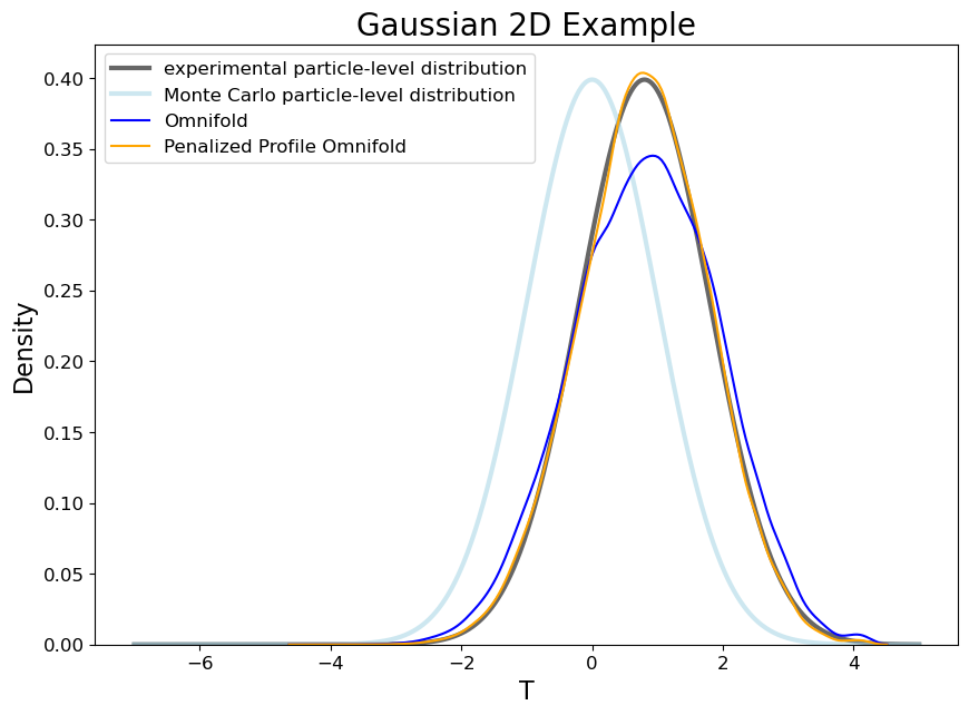
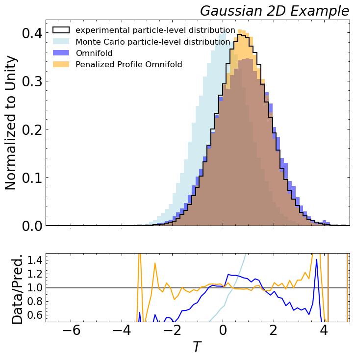
Figure 1: Results of unfolding 2D Gaussian example. Left: The unfolded particle-level density using POF (orange) and OF (blue), with both algorithms running for 5 iterations. Top-right: Unfolded spectrum aggregated into 80 bins. Bottom-right: Ratio of the unfolded spectrum to the truth spectrum.

3.1 Result

Figure 1 illustrates the results of unfolding 2D Gaussian data using both the proposed POF algorithm and the original OF algorithm. The cyan line is the Monte Carlo distribution for which the reweighting function would be applied. The results show that the original OF algorithm (blue line) deviates significantly from the true distribution (black line). This discrepancy arises because OF assumes $p(y|x)=q(y|x)$, an assumption that is invalid in the presence of incorrectly specified nuisance parameters. On the other hand, POF algorithm simultaneously optimizes the nuisance parameter along with the reweighting function. The results show that the unfolded solution (orange line) aligns closely with the truth (black line) and the fitted nuisance parameter is $\theta=1.48$ (true parameter is $1.50$). Future work will deploy standard techniques like bootstrapping to determine uncertainties.

4 Conclusion

In this work, we have proposed a new algorithm called POF, which uses machine learning to perform unfolding while also simultaneously profiling out the nuisance parameters. This relaxes the assumption in the original OF that the detector response needs to be accurately modeled in the Monte Carlo simulation and constrain the nuisance parameter in a data-driven way. At the same time, the proposed algorithm still shares similar steps as in the OF, which is easy to implement and preserving its benefits.

The results from the simple Gaussian example demonstrate the algorithm’s promising performance. Our next objective is to apply POF to more realistic examples and include critical studies like robustness, stability, and uncertainty quantification.

References

- Balasubramanian et al. [2019] Rahul Balasubramanian, Lydia Brenner, Carsten Burgard, Glen Cowan, Vincent Croft, Wouter Verkerke, and Pim Verschuuren. Statistical method and comparison of different unfolding techniques using RooFit. 2019.
- Blobel [2011] Volker Blobel. Unfolding Methods in Particle Physics. PHYSTAT2011 Proceedings, page 240, 2011. doi: 10.5170/CERN-2011-006.
- Blobel [2013] Volker Blobel. Unfolding. Data Analysis in High Energy Physics, page 187, 2013. doi: 10.1002/9783527653416.ch6. URL https://onlinelibrary.wiley.com/doi/abs/10.1002/9783527653416.ch6.
- Cowan [2002] G. Cowan. A survey of unfolding methods for particle physics. Conf. Proc., C0203181:248, 2002.
- Kuusela [2012] Mikael Kuusela. Statistical issues in unfolding methods for high energy physics. Aalto University Master’s Thesis, 2012. URL https://www.semanticscholar.org/paper/Statistical-Issues-in-Unfolding-Methods-for-High-Kuusela/d15ab0dbbeced6043cfb15d99a96e553eddadc3d.
- Arratia et al. [2022] Miguel Arratia et al. Publishing unbinned differential cross section results. JINST, 17(01):P01024, 2022. doi: 10.1088/1748-0221/17/01/P01024.
- Huetsch et al. [2024] Nathan Huetsch et al. The Landscape of Unfolding with Machine Learning. 4 2024.
- Andreev et al. [2021] V. Andreev et al. Measurement of lepton-jet correlation in deep-inelastic scattering with the H1 detector using machine learning for unfolding. 8 2021.
- H1 Collaboration [2022] H1 Collaboration. Machine learning-assisted measurement of multi-differential lepton-jet correlations in deep-inelastic scattering with the H1 detector. H1prelim-22-031, 2022. URL https://www-h1.desy.de/h1/www/publications/htmlsplit/H1prelim-22-031.long.html.
- Andreev et al. [2023] V. Andreev et al. Unbinned Deep Learning Jet Substructure Measurement in High ep collisions at HERA. 3 2023.
- H1 Collaboration [2023] H1 Collaboration. Machine learning-assisted measurement of azimuthal angular asymmetries in deep-inelastic scattering with the H1 detector. H1prelim-23-031, 2023. URL https://www-h1.desy.de/h1/www/publications/htmlsplit/H1prelim-23-031.long.html.
- LHC [2022] Multidifferential study of identified charged hadron distributions in -tagged jets in proton-proton collisions at 13 TeV. 8 2022.
- Komiske et al. [2022] Patrick T. Komiske, Serhii Kryhin, and Jesse Thaler. Disentangling Quarks and Gluons in CMS Open Data. Phys. Rev. D, 106(9):094021, 2022. doi: 10.1103/PhysRevD.106.094021.
- Song [2023] Youqi Song. Measurement of CollinearDrop jet mass and its correlation with SoftDrop groomed jet substructure observables in GeV collisions by STAR. 7 2023.
- Pani [2024] Tanmay Pani. Generalized angularities measurements from STAR at SNN = 200 GeV. EPJ Web Conf., 296:11003, 2024. doi: 10.1051/epjconf/202429611003.
- CMS [2024] Measurement of event shapes in minimum bias events from collisions at . Technical report, CERN, Geneva, 2024. URL https://cds.cern.ch/record/2899591.
- Aad et al. [2024] Georges Aad et al. A simultaneous unbinned differential cross section measurement of twenty-four +jets kinematic observables with the ATLAS detector. 5 2024.
- ATL [2024] Measurement of Track Functions in ATLAS Run 2 Data. 2024.
- Andreassen et al. [2020] Anders Andreassen, Patrick T. Komiske, Eric M. Metodiev, Benjamin Nachman, and Jesse Thaler. Omnifold: A method to simultaneously unfold all observables. Physics Reivew Letter, 124, 2020.
- Andreassen et al. [2021] Anders Andreassen, Patrick T. Komiske, Eric M. Metodiev, Benjamin Nachman, Adi Suresh, and Jesse Thaler. Scaffolding Simulations with Deep Learning for High-dimensional Deconvolution. In 9th International Conference on Learning Representations, 5 2021.
- Chan and Nachman [2023] Jay Chan and Benjamin Nachman. Unbinned Profiled Unfolding. Physical Review D, 2023. doi: https://doi.org/10.1103/PhysRevD.108.016002.
- Nachman and Thaler [2022] Ben Nachman and Jesse Thaler. Neural conditional reweighting. Physical Review D, 105, 2022.
- Kingma and Ba [2017] Diederik P. Kingma and Jimmy Ba. Adam: A method for stochastic optimization, 2017. URL https://arxiv.org/abs/1412.6980.