On interactive anisotropic walks in two dimensions generated from a three state opinion dynamics model

Abstract

A system of interacting walkers on a two-dimensional space where the dynamics of each walker are governed by the opinions of agents of a three-state opinion dynamics model are considered. Such walks, inspired by Ising-like models and opinions dynamics models, are usually considered in one-dimensional virtual spaces. Here, the mapping is done in such a way that the walk is directed along the $y$ axis while it can move either way along the $x$ axis. We explore the properties of such walks as the parameter representing the noise in the opinion dynamics model, responsible for a continuous phase transition, is varied. The walk features show marked differences as the system crosses the critical point. The bivariate distribution of the displacements below the critical point is a modified biased Gaussian function of $x,y$ which is symmetric about the $x$ axis. The marginal probability distributions can be extracted and the scaling forms of different quantities, showing power law behaviour, are obtained. The directed nature of the walk is reflected in the marginal distributions as well as in the exponents.

I Introduction

Exploring the dynamics of a physical system often involves a strategy of mapping it into an alternate realm, where new types of interacting objects or pseudo-objects are involved. Several such examples are already documented in the literature. The well-known connection between the zero-temperature spin coarsening dynamics in a one-dimensional Ising–Glauber model [1, 2, 3, 4] and the diffusive motion of domain walls, which undergo annihilation upon collision, is a notable example that has attracted significant attention. For the voter model, one can conceive of a system of coalescing walkers which is equivalent to the dynamics of the agents [5, 6, 7] in any dimension. Some of the other notable examples which got recent attention include the connection between Polya-type urn models and discrete-time random walks with memory [8, 9], as well as the connection between certain coupled oscillators and quantum algorithms [10]. These walks can be termed virtual walks as they occur in a virtual space.

Any dynamic (stochastic) process can be regarded as a walk in a virtual space, where the displacements of the walkers correspond to the dynamical variable at that time. To be precise, the position of the $i$th walker in the virtual space can be written as

$${\mathbf{r}}_{i}(t)={\mathbf{r}}_{i}(t-1)+{\mathbf{\Xi}}_{i}(t)$$ (1)

where ${\mathbf{\Xi}}_{i}$ are given in terms of the variables (e.g., spin, opinion etc.) related to the original model. For systems with many degrees of freedom, the resultant walks become interacting indirectly. Such walks have been considered earlier in quite a few studies [12, 11, 13, 14, 15]. These walks carry the signature of the phase transitions, if any, and can be related to the persistence properties of the system. It is easy to define such a walk with displacements $\pm 1$ corresponding to Ising spins or binary opinion models in a virtual one-dimensional space. When models with more than two states are considered, such walks can still be defined. In an earlier work by the present authors [14], the one-dimensional walks corresponding to the Biswas-Sen-Chatterjee (BChS henceforth) model [16] of opinion formation with three opinion states $\pm 1,0$ were generated assuming that for the zero state, the walker does not make any movement. However, this suppresses the role and effect of the “zero” states of the system and the position of the walkers will be independent of the number of times such states have been attained.

In the present work, we have considered a two-dimensional virtual walk corresponding to the three-state BChS model on a fully connected network. The walks generated will no longer be isotropic but by definition will be directed along one axis. Such directed walks in two dimensions have been considered before [17] and show ballistic behaviour at long time scales.

The results in [14] indicated the presence of a biased Gaussian distribution for the displacements below the critical point and a Gaussian above. The studies conducted here were mainly done close to the critical point. However, the dynamics of the BChS model yields a number of non-intuitive results even in absence of noise [sudip]. In the present study therefore, we allow the noise parameter to have all possible values. The deviation from a biased Gaussian becomes evident in absence of any noise as will be discussed in the present article. Hence one of the purposes is to find how far the walks are described by a biased Gaussian walk obtained earlier for general values of the noise parameter.

All information of the one dimensional walk considered in [14] are retained when the dynamics are viewed as a two dimensional virtual walk as one can recover the one dimensional distribution as marginal distribution of the 2D probability density. In addition, one can also obtain a radial distribution, which, although one dimensional in principle, will not be identical to that considered in [14].

It has been observed earlier that new exponents can be associated purely with the walk features and it will be interesting to note whether any other distinct exponents are associated with the other marginal distributions obtained from the present study which may add some more insights into the dynamics at the microscopic level. It has been further pointed out that the opinion dynamics model can be mapped to an urn model so that the present analysis has multiple applications.

II The model and definition of the virtual walks in two dimensions

In two dimensions, in general, we have a walk defined by

$${}x(t)= x(t-1)+\xi_{t}$$ (2)

$$y(t)= y(t-1)+\eta_{t}$$ (3)

$\xi_{t}$ and $\eta_{t}$ are chosen from the states of the agents of an opinion dynamics model at time t.

In the BChS model, the opinion of the $i$th individual, $o_{i}(t)$, is updated at time $t$ following an interaction with a randomly selected neighbouring agent $j$ in the following manner:

$$o_{i}(t+1)=o_{i}(t)+\mu_{ij}o_{j}(t).$$ (4)

We take the case with $o_{i}=0,\pm 1$ that may represent the support for parties with different ideologies, e.g., left, central and right, or in a two-party contest, the zero opinions can indicate neutral agents or abstainers. The opinion value is bounded, if it becomes higher (lower) than $+1$ $(-1)$ then it is made equal to $+1$ $(-1)$. The average opinion $O=\frac{\mid\sum_{i}o_{i}\mid}{N}$ can be regarded as the order parameter; note that the zero opinions do not contribute.

This model has been studied in various contexts and on different topologies [18]; we consider it on a fully connected graph. $\mu_{ij}$ is the interaction parameter representing the influence of the $j$th agent on the $i$th individual. It can take values $\pm 1$; a negative value is taken with probability $p$, the only parameter in the model.

The above mean-field model can be exactly solved yielding an order-disorder phase transition at $p=p_{c}=0.25$, with Ising-like criticality[16].

Snapshots of the trajectories of the walks of some agents is shown in Fig. 1 up to a certain time with $p<p_{c}$.

The equivalent urn model of the above mean field model has been shown in Fig. 2. Equality in distribution relations can be established between them (see Appendix A). It is noteworthy that simple adjustments to the urn rule can lead us to an urn model that shares distributional equivalence with the random walk with two memory channels (RW2MC)(see Appendix A) recently introduced in [8]. This presents an intriguing connection between a random walk with memory and a mean-field opinion dynamics model, potentially paving the way for further advancements in both domains.

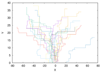
Figure 1: snapshot of trajectories of 20 walkers on XY plane for $p=0.19$ and $t=100$. The walkers, directed along the Y axis, traversed in both directions along the X axis, carrying microscopic information about the system

In the present two-dimensional walk, the position of the $i$-th walker, associated with the $i$th agent, at time step $t+1$ is determined by the following equations

$$x_{i}(t+1)=x_{i}(t)+o_{i}(t+1)$$ (5)

$$y_{i}(t+1)=y_{i}(t)+(1-\lvert o_{i}(t+1)\rvert).$$ (6)

Thus at each step the i-th walker can perform one of the three following actions: it can move to the nearest-neighbour site to its right, left or up corresponding to opinion value of the i-th individual i.e. $-1$, $0$ or $+1$ respectively.

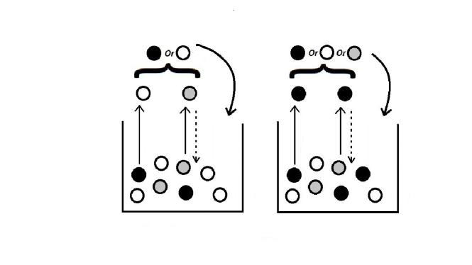
Figure 2: Pólya-type urn containing balls of three different colors and evolving by drawing two balls at a time according to the mean replacement matrix (32). The solid upward straight arrows represent random drawing of balls in each step, and the dashed downward arrows represent replacement of the drawn balls. The curved downward arrows denote addition of a new ball according to the mean replacement matrix (32.)

III Results

We performed numerical simulations of the kinetic exchange model for opinion dynamics on a fully connected graph with N nodes. The initial configuration was entirely random, i.e. at time $t=0$, the number of individuals holding opinions of $0$, $+1$, and $-1$ was evenly distributed, with each opinion being assigned to $N/3$ individuals. One Monte Carlo Step (MCS) consists of N updates. During each update, two distinct individuals are selected at random, and the opinion of the first individual is modified based on the rules specified in Eq. 4 .The maximum system size simulated is N = 2000 and the maximum number of configurations over which averaging has been done is 200000.

III.1 2D walk distribution

The bivariate probability density function of the 2D virtual walk, $S(x,y,t)$, for the position $x$, $y$ of the walkers at time $t$ is estimated from the numerical simulation. For brevity, we suppress the argument $t$ in the following.

We have found that for $p<p_{c}$, the bivariate probability density function can be fitted to the following modified bivariate normal distribution (see Fig. 3(a) which shows the results for positive values of $x$ only):

$$S(x,y)=H(x,y)e^{-z(x,y)}$$ (7)

where

$$z(x,y)=l(x-\mu_{1})^{2}+d(y-\mu_{2})^{2}+u(x-\mu_{1})(y-\mu_{2})\\$$ (8)

and

$$H(x,y)\propto\left\{1+w\operatorname{erf}(h_{1}(x-\mu^{\prime}_{1})+h_{2}(y-\mu^{\prime}_{2}))\right\}.$$ (9)

For $p>p_{c}$, the 2D probability density function of the walk can be fitted to a bivariate normal distribution of the following form with zero correlation,

$$S_{c}(x,y)=Ke^{-ex^{2}-f(y-\mu_{c})^{2}},$$ (10)

i.e., a bivariate Gaussian distribution with centre at $x=0,y=\mu_{c}$. The behaviour is shown in (Fig. 3(b)). The distributions in Eq. (7) and Eq. (10) are for a particular time $t$ and the coefficients that appear in Eq. 8, Eq. 9 and Eq. 10 have an explicit dependence on $t$.

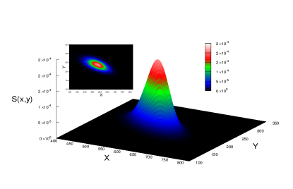
(a)

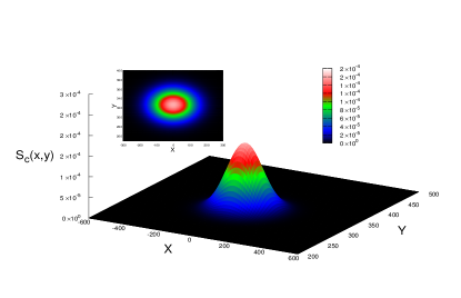
(b)

Figure 3: (a)$S(x,y)$ for positive x for $p=0.19$, $N=1000$ and $t=1000$. inset shows the 2D projection on the xy plane from which departure from bivariate normal distribution can be seen. (b) $S_{c}(x,y)$ for $p=0.25,N=1000,t=1000.$. inset shows the 2D projection on the xy plane, from which similarity with bivariate normal distribution can be seen

The modified bivariate normal form of $S(x,y)$ (eq. 7) has been confirmed by a quantile-quantile (q-q) plot (Fig. 4). The q-q plot provides a visual method to assess whether two data sets are derived from populations that share a common distribution. If the two sets come from a population with the same distribution, the points should fall approximately along a 45-degree straight line. The more the deviation from this line, the stronger the indication that the two data sets originate from populations with distinct distributions. For example, if we try to fit the observed bivariate distribution from simulation to a bivariate normal distribution with nonzero correlation, i.e.,

$$G(x,y)=Ae^{-a(x-\nu_{x})^{2}-b(y-\nu_{y})^{2}-c(x-\nu_{x})(y-\nu_{y})}$$ (11)

then the corresponding q-q plot deviates from the 45-degree reference line (Fig. 4) but the deviations of the bivariate modified Gaussian form of Eq. (7) are much smaller.

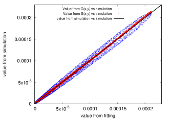
Figure 4: q-q plot for the fitting of the bivariate walk distribution at $p=0.19$ with bivariate normal distribution $G(x,y)$ (eq.11) and $S(x,y)$ (eq.7). The q-q plot clearly shows that the data for the bivariate distribution $S_{c}(x,y)$ (denoted by red dot) is matched to the reference line much better than the bivariate normal distribution $G(x,y)$ (denoted by blue dot).

Marginal probability densities of the bivariate distribution functions along the X and Y axis can be defined as,

$$P_{x}(x,t)=\sum_{y=0}^{\infty}S(x,y,t)$$ (12)

and

$$P_{y}(y,t)=\sum_{x=0}^{\infty}S(x,y,t)$$ (13)

where in the last equation, we have utilised the symmetry and defined $P_{y}$ for positive values of $x$ only.

Angular marginalization refers to marginalizing the bivariate distribution to yield 1-D distributions over radius $r$ which is the distance from the origin. Radial marginalized distribution of $S(x,y,t)$ can be defined as follows

$$P_{r}(r,t)=\sum_{x=0}^{\infty}\sum_{y=0}^{\infty}\delta_{r,\lfloor\sqrt{x^{2}+y^{2}}\rfloor}S(x,y,t).$$ (14)

where also the symmetry $x\to-x$ has been used.

III.2 Results for $p=0$

We report first the results of the one-dimensional walk corresponding to $p=0$. The persistent probability can also be obtained for agents whose initial opinion is $\pm 1$.

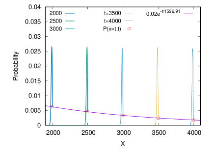
Figure 5: At $p=0$ marginal distributions along the X-axis $P_{0}(x,t)$ for different times are shown. fitting of the endpoints i.e. $P(x=t,t)$, which is equal to the persistence probability along the positive X-axis or persistence probability of $+1$ opinions can be achieved with the curve (violate line) of the form $e^{-\frac{t}{\tau_{1}}}$, where $\tau_{1}=1596.91$

We define the marginal probability density along the X and Y axes according to Eq. 12 and Eq. 13 and for $p=0$ denoted them by $P_{0}(x,t)$ and $Q_{0}(y,t)$ respectively. Fig. 6(b) and Fig. 7(b) clearly show that the distributions are non-Gaussian. On the other hand, we show in the inset of the figures as an example that for a small value $p=0.05$, the distributions are apparently a (biased) Gaussian. So, a change in behaviour due to disorder is noticed. Further, we have succeded in doing data collapses for different times ( Fig. 6(a) and Fig. 7(a)). From Fig. 6(a) it is evident that $P_{0}(x,t)$ has the following modified Gaussian form

$$P_{0}(x,t)\propto\frac{f_{0}(z_{0})}{\log t}e^{-\alpha_{0}z_{0}^{2}}$$ (15)

Where $z_{0}=\frac{x-\lambda_{0}t}{\log t}$ and

$$f_{0}(z_{0})\propto\left(1+b_{1}\operatorname{erf}(b_{2}(z_{0}-b_{3}))\right)$$ (16)

On the other hand from Fig. 7(a) it is evident that $Q_{0}(y,t)$ has the following modified Gaussian form

$$Q_{0}(y,t)=\frac{q_{0}(v_{0})}{t^{0.23}}e^{-\beta_{0}v_{0}^{2}}$$ (17)

Where $v_{0}=\frac{x-\omega_{0}t^{0.98}}{t^{0.23}}$ and

$$q_{0}(v_{o})\propto\left(1+k_{1}\operatorname{erf}(k_{2}(v_{0}-k_{3}))\right)$$ (18)

According to the definition of the walking scheme, the persistence probability $R_{x}(t)$ of the walker along the positive and negative X-axis is the persistence probability for opinions $+1$ and $-1$ respectively and related to $P_{0}(x,t)$ by the equation $P_{x}(x=t,t)=P_{x}(x=-t,t)=R_{x}(t)$. the persistence probability of the walker along the positive Y-axis denoted by $R_{y}(t)$ is the persistence probability for opinions $0$ and related to $Q_{0}(y,t)$ by the equation $Q_{0}(y=t,t)=R_{y}(t)$. $R_{x}(t)$ and shows exponential decay over time i.e. $R_{x}(t)\propto e^{-\frac{t}{\tau_{1}}}$ and $R_{y}(t)\propto e^{-\frac{t}{\tau_{0}}}$ , as illustrated in Fig. 5 and Fig. 8 respectively.

III.3 Results for $p\neq 0$

$P_{x}(x,t)$, is the marginal probability distribution along the X axis and also identical to the probability distribution of the 1D virtual walk [14]. For nonzero p we find zero persistence along both X and Y axis. Now according to the previous study [14] of the present authors, it is expected to take the form of a biased Gaussian for $0<p<p_{c}$. But motivated by the modified Gaussian form of distributions for $p=0$ we have the distributions more precisly (averaging over 200000 configurations) which clearly shows that $P_{x}(x,t)$ has a biased modified Gaussian form. We find that a nice collapse can be obtained for $0<p<p_{c}$ by plotting $P_{x}(x,t)\sqrt{t}$ against $z_{x}=\frac{(x-\gamma_{x}t)}{\sqrt{t}}$ fig. 12. We have also estimated the relative error with a Gaussian fitting curve and found that the errors are significant. Fitting with a modified Gaussian improves the precision [fig. 12].

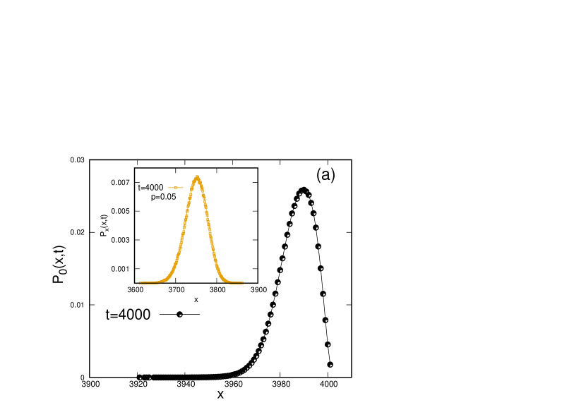
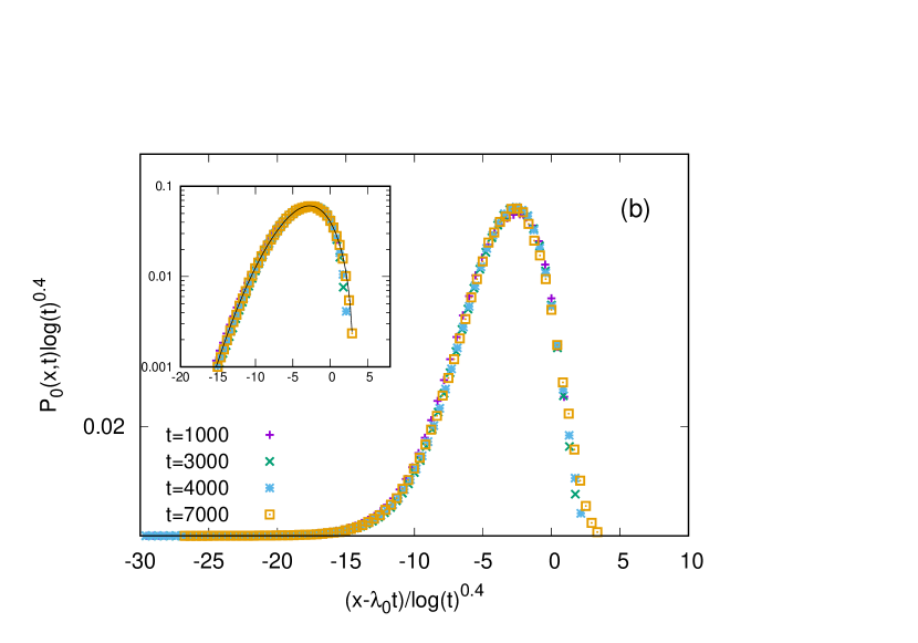
Figure 6: (a) $P_{0}(x,t)$ of the walk along the X axis for $p=0.05$ and $t=4000$. A comparison with $p=0.05$ clearly shows a change in the behaviour of the marginal distribution along the X-axis. For $p=0.05$ (inset) it looks like a Gaussian but for $p=0$ it is a modified Gaussian. (b) Data collapse of $P_{0}(x,t)(\log t)^{0.4}$ for different times at $p=0$ and $x>0$ plotted against the scaling variable $z_{0}=\frac{x-\lambda_{0}t}{(\log t)^{0.4}}$. Where $\lambda_{0}\sim 0.999$. The inset shows the data collapse in the log scale. fitting with a modified Gaussian form of Eq. 15 for $t=7000$ has been shown in the inset with a black line. We observed in Fig. 8 that the endpoints for $z_{0}>0$ which is related to persistence probability and denote $P_{0}(x=t,t)(\log t)^{0.4}$, do not follow the time evolution of the distribution but decrease independently as time progresses.

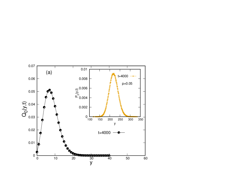
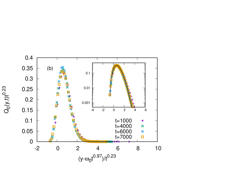
Figure 7: (a) $Q_{0}(y,t)$ of the walk along the Y axis for $t=4000$. A comparison with $p=0.05$ clearly shows a change in the behaviour of the marginal distribution along the Y-axis. For $p=0.05$ (inset) it looks like a Gaussian and for $p=0$ but for $p=0$ it is a modified Gaussian. (b) Data collapse of $Q_{0}(y,t)t^{0.23}$ for different times at $p=0$ plotted against the scaling variable $v_{0}=\frac{x-\omega_{0}t^{0.97}}{t^{0.23}}$. Where $\omega_{0}\sim 0.001$ . The inset shows the data collapse in the log scale. fitting with a modified Gaussian form of Eq. 17 for $t=7000$ has been shown in the inset with a black line. We observed in Fig. 8 that the endpoints for $v_{0}<0$ which is related to persistence probability and denote $Q_{0}(y=t,t)t^{0.23}$, do not follow the time evolution of the distribution but decrease independently as time progresses.

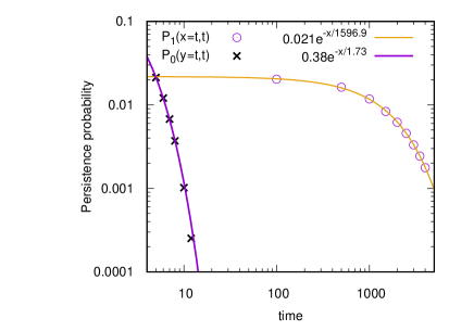
Figure 8: At $p=0$ the endpoints of the marginal distributions along the positive X and Y axis i.e. $P_{0}(x=t,t)$ and $Q_{0}(y=t,t)$ respectively, which is equal to the persistence probability along the axes or persistence probability of $+1$ and $0$ opinions are shown to decreases exponentially as time progresses. Fitting of the persistence probabilities can be achieved in the forms proportional to $e^{-\frac{t}{\tau_{1}}}$ and $e^{-\frac{t}{\tau_{0}}}$ (denoted by yellow and violate line respectively), where $\tau_{1}=1596.9$ and $\tau_{0}=1.73$. This behaviour is independent of the time evolution of the distributions to which they belong.

The modified Gaussian form can be written as follows.

$$P_{x}(x,t)=\frac{f(z_{x})}{\sqrt{t}}e^{-\alpha z_{x}^{2}}$$ (19)

where $z_{x}\propto\frac{(x-\gamma_{x}t)}{\sqrt{t}}$. $\gamma_{x}$ and $\alpha$ are functions of $p$ and $f(z_{x})=1+w_{1}\operatorname{erf}{(w_{2}(z_{x}-w_{3}))}$ which has the same form as Eq. 16 for $p=0$. So, the walk deviates from the biased random walk for $p<p_{c}$. But the time scaling is different from $p=0$ which is due to the incorporation of noise.
A similar type of data collapse can be achieved for $P_{y}(y,t)$ (Fig. 10) and $P_{r}(r,t)$(Fig. 11) by comparing the relative errors with Gaussian fit one can write

$$P_{y}(y,t)=\frac{q(z_{y})}{\sqrt{t}}e^{-\beta z_{y}^{2}}$$ (20)

where $z_{y}=\frac{(y-\gamma_{y}t)}{\sqrt{t}}$ and $m(z_{r})$ has similar form as $f(z_{x})$. But one thing is to be noted that according to the definition of $P_{r}(r,t)$ in Eq. 14 constraining r only to the integers all the points between r and r+1 sum up to build $P_{r}(r,t)$ as a result noise can not be avoided and we observe modified Gaussian fit to $P_{r}(r,t)$ slightly better than Gaussian fit (Fig. 11) which is not sufficient to conclude whether it is Gaussian or modified Gaussian.

Above criticality ($p>p_{c}$), the marginal distribution along the X-axis should behave like an unbiased random walk and along the Y-axis should behave like a biased random walk which is evident from the bivariate distribution for $p>p_{c}$ i.e. Eq. 10. We have also observed that. Data collapse of the marginal distribution along the X-axis $P_{c}(x,t)$ has been shown in Fig. 12. One can write

$$P_{xc}(x,t)\propto\frac{1}{\sqrt{t}}e^{-\frac{\alpha_{c}x^{2}}{t}}$$ (21)

with $Var(x)\propto t$.marginal distribution along the Y-axis $P_{yc}(y,t)$ still survives with a bias but now has a Gaussian profile. It can be written as

$$P_{yc}(y,t)\propto\frac{1}{\sqrt{t}}e^{-\frac{\beta_{c}y^{2}}{t}}$$ (22)

with $Var(y)\propto t^{2}$.
$P_{rc}(r,t)$ for bivariate normal distribution corresponding to a bivariate normal distribution Eq.11 with mean$\nu_{x}=0,\nu_{y}=\mu_{c}$,and standard deviation $\zeta_{x}\neq\zeta_{y}$ and zero covariance can be written as [31, 32]

$$P_{rc}(r,t)=D(r,t)e^{-\frac{r^{2}(\zeta_{x}^{2}+\zeta_{y}^{2})}{4\zeta_{x}^{2}\zeta_{y}^{2}}}$$ (23)

where,

$$D(r,t)=h\{I_{0}(vr^{2})I_{0}(gr)+2\sum_{k=1}^{\infty}I_{k}(vr^{2})I_{2k}(gr)cos(2k\psi)\}$$

$I_{n}$ ($n\in\mathbb{Z}$) is the modified Bessel function of the first kind. $v,g$ and $\psi$ depend on $\mu_{y},\sigma_{x}$ and $\sigma_{y}$ which are functions of time only. As a result for $P_{r}^{\prime}(r,t)$ we have not observed a data collapse like $P_{xc}(x,t)$, nor have we encountered the modified form.

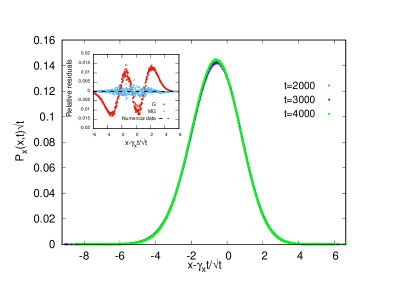
Figure 9: Data collapse of $P_{x}(x,t)\sqrt{t}$ for $p=0.19$ and $x>0$ plotted against the scaling variable $z_{x}=\frac{x-\gamma_{x}t}{\sqrt{t}}$ where $\gamma_{x}\sim 0.605$. The inset shows relative residuals for Gaussian (G) fit and a modified Gaussian (MG) (Eq.19) fit. Relative residuals of the fittings are defined by $\frac{P_{x}(x,t)\sqrt{t}-(fitted\,\,function)}{P_{x\mid max}(x,t)}$ where $P_{x\mid max}(x,t)$ denotes the maximum value of $P_{x}(x,t)$. The numerical data are shown as a long-dashed black curve and the red and blue dots refer to the G and MD fit respectively. Non-negligible residuals for G confirm a modified Gaussian form of $P_{x}(x,t)$ which leads to a modified Gaussian marginal distribution along the X-axis.

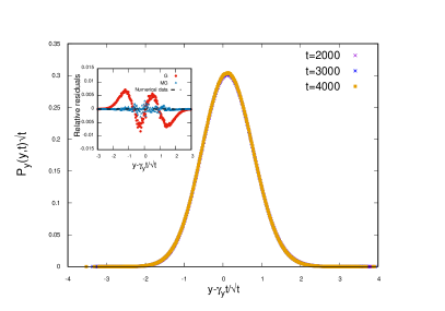
Figure 10: Data collapse of $P_{y}(y,t)\sqrt{t}$ for $p=0.19$ plotted against the scaling variable $z_{y}=\frac{y-\gamma_{y}t}{\sqrt{t}}$ is shown , where $\gamma_{y}\sim 0.235$. According to the definition provided in Eq. (6), $y$ must be greater than zero throughout the walk. The inset shows relative residuals for Gaussian (G) fit and a modified Gaussian (MG) (Eq.20) fit. Relative residuals of the fittings are defined by $\frac{P_{y}(y,t)-(fitted\,\,function)}{P_{y\mid max}(y,t)}$, where $P_{y\mid max}(y,t)$ denotes the maximum value of $P_{y}(y,t)$. The numerical data are shown as a long-dashed black curve and the red and blue dots refer to the G and MD fit respectively. Non-negligible residuals for G confirm a modified Gaussian form of $P_{y}(y,t)$ which leads to a modified Gaussian marginal distribution along the Y-axis.

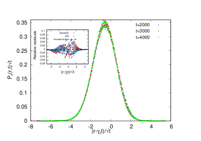
Figure 11: Data collapse of $P_{r}(r,t)\sqrt{t}$ plotted against the scaling variable $z_{r}=\frac{r-\gamma_{r}t}{\sqrt{t}}$ is shown for $p=0.19$, where $\gamma_{r}\sim 0.65$. A Gaussian fit (black line) has been shown which deviates from numerical data. The inset shows relative residuals for Gaussian (G) fit and a modified Gaussian (MG) (Eq.LABEL:mgr) fit. Relative residuals of the fittings are defined by $\frac{P_{r}(r,t)-(fitted\,\,function)}{P_{r\mid max}(r,t)}$, where $P_{r\mid max}(r,t)$ denotes the maximum value of $P_{r}(r,t)$.

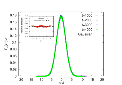
Figure 12: Data collapse of $P_{c}(x,t)\sqrt{t}$ for $p=0.26$ and $x>0$ plotted against $\frac{x}{\sqrt{t}}$. A Gaussian fit (black line) for $t=1000$ has been shown. The inset shows the relative residuals of the fittings. The numerical data are shown as a long-dashed black curve and the red dots refer to the Gaussian fit. residuals are negligible which confirms a Gaussian form of $P_{c}(x,t)$.

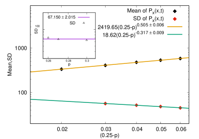
Figure 13: Variation of mean and SD of $P_{x}(x,t)$ against $p_{c}-p$ for $p<p_{c}$. The values of the critical exponents are $0.505$ and $-0.317$ respectively. A comparison of different exponents and parameters of marginal distributions are shown in Table LABEL:table1. The inset shows SD for $p>p_{c}$ which becomes constant.

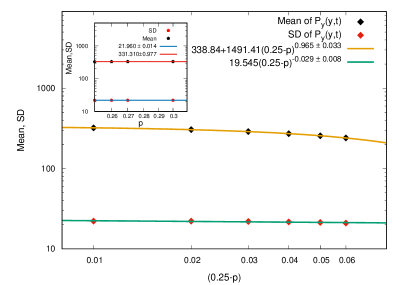
Figure 14: Variation of mean and SD of $P_{y}(y,t)$ against $p_{c}-p$ for $p<p_{c}$. The values of the critical exponents are $0.965$ and $-0.029$ respectively. A comparison of different exponents and parameters of marginal distributions are shown in Table LABEL:table1. The inset shows Mean and SD for $p>p_{c}$ which becomes constant.

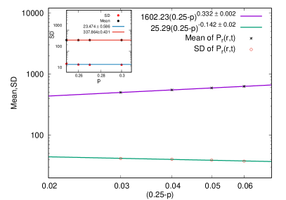
Figure 15: Variation of mean and SD of $P_{r}(r,t)$ against $p_{c}-p$ for $p<p_{c}$. The values of the critical exponents are $0.332$ and $-0.142$ respectively. The inset shows Mean and SD for $p>p_{c}$ which becomes constant.

Next, we examined the variations of the mean and standard deviations of the marginal distributions for $0<p<p_{c}$ and $p>p_{c}$ as a function of $(p_{c}-p)$. As we approach the critical point ($p_{c}=0.25$), it is anticipated that the mean value of $P_{x}(x,t)$ appeared in Eq. 19 should approach zero and for $p>p_{c}$ bias in the marginal Gaussian distribution along X axis becomes zero as noted in Eq. 21. We note by analyzing the data that (Fig. 13) the mean of $P_{x}(x,t)$

$$M_{x}\propto(p_{c}-p)^{\delta_{1}};$$ (24)

where $\delta_{1}\sim 0.5$ and the standard deviation (SD)

$$W_{x}\propto(p_{c}-p)^{-\sigma_{1}};$$ (25)

where $\sigma_{1}\sim 0.32$. Critical exponents corresponding to the mean and variance of $P_{x}(x,t)$ [Fig. 14] and $P_{r}(r,t)$ [Fig. 15] have also been obtained.

Mean of $P_{x}(x,t)$ behaves as follows

$$M_{y}\propto(p_{c}-p)^{\delta_{2}};$$ (26)

where $\delta_{2}\sim 0.96$ and the SD of $P_{y}(y,t)$

$$W_{y}=w_{1}+w_{2}(p_{c}-p)^{-\sigma_{2}};$$ (27)

where $\sigma_{2}\sim 0.03$ and $w_{1},w_{2}$ are constants. Mean of $P_{r}(r,t)$ behaves as follows

$$M_{r}\propto(p_{c}-p)^{\delta_{3}};$$ (28)

where $\delta_{3}\sim 0.33$ and the SD of $P_{r}(r,t)$

$$W_{r}\propto(p_{c}-p)^{-\sigma_{3}};$$ (29)

where $\sigma_{3}\sim 0.14$
For $p>p_{c}$ SD and mean becomes constant a p increases.

From the definition of the walk Eq.3

From the definition (Eq. 5 and Eq. 6) of the random walks it follows that $\eta_{t}$ and $\xi_{t}$ of Eq.3 are not independent random variables. If $\eta_{t}$ is $1$ or $-1$ then $\xi_{t}$ is $0$, otherwise $\xi_{t}$ is $1$. The covariance between $\eta_{t}$ and $\zeta_{t}$ can be defined as $Cov(\eta_{t},\xi_{t})=\langle\eta_{t},\xi_{t}\rangle-\langle\eta_{t}\rangle\langle\xi_{t}\rangle$
which is, equal to $-\langle\eta_{x}\rangle\langle\xi_{y}\rangle$ in our case as both can not be nonzero at the same time. But for $p>p_{c}$ in addition to that $\langle\eta_{x}\rangle=0$ i.e. $Cov(\eta_{x},\xi_{y})$ becomes zero. So, effectively $\eta_{x}$ and $\xi_{y}$ become independent for $p>p_{c}$. correlation coefficient $\Omega$ between $\eta_{x}$ and $\xi_{y}$ can be written as

$$\Omega=\frac{cov(\eta_{x},\xi_{y})}{\sqrt{Var(\eta_{x})Var(\xi_{y})}}$$

By calculating $\Omega$ from the simulation data, we have found that (Fig. 16),

$$\Omega\propto-(p_{c}-p)^{0.4}$$

So, $\eta_{x}$ and $\xi_{y}$ are negatively correlated as expected. It is interesting to note that such a kind of correlation can give rise to a nontrivial bivariate distribution of Eq.7 for $p<p_{c}$.

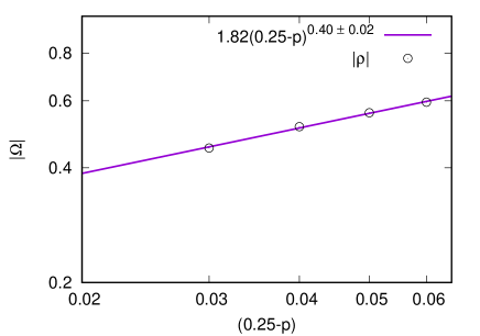
Figure 16: Variation of the absolute value of correlation coefficient $|\Omega|$ between $\eta_{x}$ and $\xi_{y}$ with $(p_{c}-p)$ for $p=0.19$. The value of the critical exponent is $\sim 0.4$.

The conditional mean along the $Y$ axis, for a given position along the $X$ axis, is defined as follows.

$$\eta_{Y|X}(x,t)=\sum_{y=0}^{\infty}yS(x,y,t)$$ (30)

Which can be fitted to the following form for particular p and t. (Fig.17).

$$v(x)=k_{y}+l_{1}(x-k_{x})+l_{2}(x-k_{x})^{2}+l_{3}(x-k_{x})^{3}$$ (31)

Where $k_{x}$ and $k_{y}$ are very close to $\alpha t$ and $\beta t$ respectively. In Fig. 17 we have shown the conditional mean for $p=0.19$. One can obtain a similar kind of behaviour for conditional mean along the X axis also. It should be noticed that for bivariate normal distribution (Eq.11), the conditional mean is a linear function of x (i.e. $\eta_{Y|X}=\nu_{y}+l(x-\nu_{x})$) So, a departure of $\eta_{Y|X}$ from the linear dependence on x is also a piece of evidence for the modified normal distributions of $S(x,y,t)$ for $p<p_{c}$.

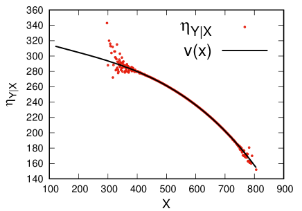
Figure 17: The conditional mean along the $Y$ axis, $\eta_{Y|X}$ for $p=0.19$, $N=1000$ and $t=1000$ is fitted with the functional form $v(x)=k_{y}+l_{1}(x-k_{x})+l_{2}(x-k_{x})^{2}+l_{3}(x-k_{x})^{3}$, where $k_{y}\sim 234.65$ which is very close to $\beta t\sim 235$ (Fig. 14), $k_{x}\sim\alpha t\sim 605$ and $l_{1}\sim-0.296$, $l_{2}\sim-4\times 10^{-4}$, $l_{3}\sim 3.8\times 10^{-7}$.

IV Conclusions

A new kind of walk in 2D space has been introduced in the present paper inspired by an opinion dynamics model. While such walk models have been studied earlier in one dimension, the present walk, studied in 2 dimensions for the first time to the best of our knowledge, incorporates anisotropy as well. The extension to two dimensions naturally reveals a more detailed picture of the microscopic feature. Our main purpose of study of the virtual walk is to see whether any nontrivial property of the system can be revealed using the Probability density function of the walkers which can provide new physical insights. The dynamics of zero opinion were suppressed in 1D virtual walks but when viewed in 2D it came out of the compressed state and became visible as marginal distribution along the Y axis. The probability densities of the 1D walk for $0<p<p_{c}$ appeared to be biased Gaussian in our previous study. Observing modified biased Gaussian marginal distributions we have conducted a more precise study which shows that it is indeed a modified biased Gaussian for $p_{c}>p>0$ also but the modifications are quite small compared to $p=0$. On one hand, our findings reveal a new result that incorporating noise significantly reduces the deviation from a biased Gaussian distribution. On the other hand, the alteration of the time evolution of the marginal distributions along the X and Y axes in a fundamentally different manner as a result of noise incorporation represents a non-intuitive behaviour. Correlations in interacting particle models are usually defined for higher dimensional systems. Here we have studied the correlations between two random variables representing the 2D virtual walker’s step along the X and Y axis and found that they are negatively correlated and a corresponding critical exponent is obtained. Different critical exponents corresponding to the marginal distributions can define universality class for three-state interacting spin systems which can be compared in future with other three-state spin systems to see whether they belong to the same universality class or not.

V Acknowledgments

S.S acknowledge support by the Council of Scientific and Industrial Research, Government of India, through a CSIR NET fellowship [CSIR JRF Sanction No. 09/028(1134)/2019-EMR-I] and P.S acknowledge support by the Council of Scientific and Industrial Research, Government of India, through project no. 03/1495/23/EMR-II.

Appendix A Equivalent urn model

Let us introduce a discrete-time urn model with balls of three colors. Assume the three colors to be black (B), white (W ), and gray (G). The composition of the urn at time $t$ is given by a set $N_{t}=(N^{B}_{t},N^{W}_{t},N^{G}_{t})$ where $N^{B}_{t}$, $N^{W}_{t}$ and $N^{G}_{t}$ counts the number of black, white and grey balls respectively. We start at $t=0$ with $N=N^{B}_{0}+N^{W}_{0}+N^{G}_{0}$ balls. Suppose at each time step two balls were taken out one after the other from the urn. Then the possible outcomes of any drawing can be represented by the following ordered sets: [B, B], [B, W], [W, B], [W, W], [G, W], [W, G], [G, B], [B, G] and [G, G]. After observing the drawn pair, the first ball from it is reinserted into the urn, and a B, W, or G ball is added to it. So, as time increases The total number of balls remains constant. The selection of the ball to be added to the urn is determined by the drawn pair, as outlined in the mean replacement matrix below.

$$\blockarray{cccc}&\>\>BWG\\ \block{c(ccc)}BB\>\>\,a\>0\>b\>\\ BW\>\>\,b0a\\ WB\>\>\,0ba\\ BG\>\>\,100\\ GB\>\>\,ab0\\ WW\>\>\,0ab\\ WG\>\>\,010\\ GW\>\>\,ba0\\ GG\>\>\,001\\$$ (32)

Here $a+b=1$. The elements of the matrix represent the conditional probability of the colored ball added in each step. The urn described above belongs to the Pólya type urns evolving by two drawings with randomized replacement rules. If we associate $+1$ to black balls, $-1$ to white balls and $0$ to gray balls then the mean replacement matrix (32) can be obtained for the choice $a=1-p$ and $b=p$ from Eq.(4).
We define $M_{t}=\frac{\langle N^{B}_{t}-N^{W}_{t}\rangle}{N}$ as the order parameter of the system. One can show that for a particular $p$,

$$Number\>of\>+1\>opinions\>at\>time\>t=_{d}N^{B}_{t}$$ (33)

$$Number\>of\>-1\>opinions\>at\>time\>t=_{d}N^{W}_{t}$$ (34)

$$Number\>of\>0\>opinions\>at\>time\>t=_{d}N^{G}_{t}$$ (35)

and,

$$O(t)=_{d}M_{t},$$ (36)

where $=_{d}$ implies equality in law or equality in distribution. That is to say, the difference between the number of black and white balls in the urn at time $t$ follows the same distribution as the order parameter at time t of the kinetic exchange model of opinion dynamics defined on a fully connected graph by the eq.4 with $N$ individuals and $N^{B}_{0}$, $N^{W}_{0}$, $N^{G}_{0}$ number of $+1$, $-1$ and $0$ individuals respectively at time $t=0$.

References

- [1] Privman V. 1997 Nonequilibrium Statistical Mechanics in One Dimension (Cambridge University Press, Cambridge).
- [2] Derrida B, Bray AJ and Godrèche C. 1994 Non-trivial exponents in the zero temperature dynamics of the 1D Ising and Potts models J. Phys. A 27, L357.
- [3] Derrida B. 1995 Exponents appearing in the zero-temperature dynamics of the 1D Potts model. J. Phys. A Math. Theor. 28, 1481.
- [4] Derrida B, Hakim V, Pasquier V. 1995 Exact First-Passage Exponents of 1D Domain Growth: Relation to a Reaction-Diffusion Model. Phys. Rev. Lett. 75, 751.
- [5] Liggett TM. 1985 Interacting Particle Systems (Springer, New York).
- [6] Krapivsky PL, Redner S, Ben-Naim E. 2010 A Kinetic View of Statistical Physics. (Cambridge University Press, Cambridge).
- [7] M. Howard, C. Godrèche, Persistence in the Voter model: continuum reaction-diffusion approach, J. Phys. A 31, L209 (1998).
- [8] Saha S. Random walk with multiple memory channels, Phys. Rev. E 106, L062105 (2022).
- [9] Erich Baur and Jean Bertoin Elephant random walks and their connection to Pólya-type urns, Phys. Rev. E 94, 052134 (2016).
- [10] Ryan Babbush, Dominic W. Berry, Robin Kothari, Rolando D. Somma, and Nathan Wiebe, Exponential Quantum Speedup in Simulating Coupled Classical Oscillators, Phys. Rev. X 13, 041041 (2023).
- [11] J.M. Drouffe, C. Godrèche, Stationary definition of persistence for finite-temperature phase ordering, Journal of Physics A: Mathematical and General 31, 9801 (1998).
- [12] J.M. Drouffe, C. Godrèche, Temporal correlations and persistence in the kinetic Ising model: the role of temperature, The European Physical Journal B-Condensed Matter and Complex Systems 20, 281 (2001).
- [13] P. Mullick, P. Sen, Virtual walks in spin space: A study in a family of two-parameter models, Phys. Rev. E 97, 052122 (2018).
- [14] S. Saha, P. Sen, Virtual walks inspired by a mean-field kinetic exchange model of opinion dynamics, Philosophical Transactions of the Royal Society A, 380, 20210168 (2022).
- [15] K. Biswas and P. Sen, Virtual walks and phase transitions in two dimensional BChS model with extreme switches, Phys. Rev. E (in press).
- [16] Biswas S, Chatterjee A, Sen P, Disorder induced phase transition in kinetic models of opinion dynamics. Physica A 391, 3257 (2012).
- [17] Sheng-You Huang, Xian-Wu Zou, and Zhun-Zhi Jin,Directed random walks in continuous spacePhys. Rev. E 65, 052105 (2002).
- [18] Biswas S, Chatterjee A, Sen P, Mukherjee S and Chakrabarti BK Social dynamics through kinetic exchange: the BChS model, Front. Phys. 11:1196745 (2023). –
- [19] C. Castellano, S. Fortunato, V. Loreto, Statistical physics of social dynamics, Rev. Mod. Phys. 81, 591 (2009).
- [20] S. Galam, Sociophysics: A Physicist’s Modeling of Psycho-political Phenomena, Springer, Boston, MA (2012).
- [21] P. Sen, B.K. Chakrabarti, Sociophysics: An Introduction, Oxford University Press (2014)
- [22] C. Castellano, S. Fortunato, V. Loreto, Statistical physics of social dynamics, Rev. Mod. Phys. 81, 591 (2009).
- [23] S. Galam, Sociophysics: A Physicist’s Modeling of Psycho-political Phenomena, Springer, Boston, MA (2012).
- [24] P. Sen, B.K. Chakrabarti, Sociophysics: An Introduction, Oxford University Press (2014).
- [25] G. Toscani, P. Sen, and S. Biswas, eds. Kinetic exchange models of societies and economies, Philosophical Transactions of the Royal Society A 380, 20210170 (2022).
- [26] B. Derrida, A.J. Bray, C. Godrèche Non-trivial exponents in the zero temperature dynamics of the 1D Ising and Potts models J. Phys. A 27, L357 (1994).
- [27] B. Derrida, Exponents appearing in the zero-temperature dynamics of the 1D Potts model. J. Phys. A Math. Theor. 28, 1481 (1995).
- [28] B. Derrida, V. Hakim, V. Pasquier, Exact First-Passage Exponents of 1D Domain Growth: Relation to a Reaction-Diffusion Model. Phys. Rev. Lett. 75, 751 (1995).
- [29] V. Privman, Nonequilibrium Statistical Mechanics in One Dimension, Cambridge University Press, Cambridge (1997).
- [30] S. Goswami, A. Chatterjee, P. Sen, Antipersistent dynamics in kinetic models of wealth exchange, Physical Review E 84, 051118 (2011).
- [31] Emily A. Cooper and Hany Farid,A Toolbox for the Radial and Angular Marginalization of Bivariate Normal Distributions, arXiv:2005.09696 (2022)
- [32] Weil H, The distribution of radial error, The Annals of Mathematical Statistics, pp.168–170 (1954)