3D ISM structure challenges the Serkowski relation

Abstract

Context. The Serkowski relation is the cornerstone of studies of starlight polarizations as a function of wavelength. Although empirical, its extensive use since its inception by Serkowski et al. (1975) to describe polarization induced by interstellar dust has elevated the relation to the status of an indisputable “law”: this is the benchmark against which models of interstellar dust grains are validated.

Aims. We revisit the effects of the three - dimensional structure of the interstellar medium (ISM) on the wavelength dependence of interstellar polarization.

Methods. We use analytical models to show how the wavelength dependence of both the polarization fraction and direction is affected by the presence of multiple clouds along the line of sight (LOS). We account for recent developments in dust distribution modelling and we utilize an expanded archive of stellar polarization measurements to establish the effect of multiple clouds along the LOS. We highlight concrete examples of stars whose polarization profiles are severely affected by LOS variations of the dust grain and magnetic field properties, and we provide a recipe to accurately fit multiple cloud Serkowski models to such cases.

Results. We present, for the first time, compelling observational evidence that the three - dimensional structure of the magnetized ISM often results to the violation of the Serkowski relation. We show that three - dimensional effects impact interstellar cloud parameters derived from Serkowski fits. In particular, the dust size distribution in single - cloud sightlines may differ from analyses that ignore 3D effects, with important implications for dust modelling in the Galaxy.

Conclusions. Our results suggest that multiwavelength stellar polarization measurements offer an independent probe of the LOS variations of the magnetic field orientation, and thus constitute a potentially valuable new tool for the 3D cartography of the interstellar medium. Finally, we caution that, unless 3D effects are explicitly accounted for, a poor fit to the Serkowski relation does not, by itself, constitute conclusive evidence that a star is intrinsically polarized.

1 Introduction

Dust is ubiquitous in the interstellar medium (ISM) of our Galaxy and plays a significant role in many astrophysical processes. The thermal (gray-body) emission of interstellar dust spans many frequencies (100 – 1000 GHz), making dust a powerful tracer of the morphology of ISM structures as well as a diagnostic of their physical properties, such as temperature (Hildebrand, 1983; André et al., 2010). At the same time dust emission poses a challenge for cosmological experiments because it veils the cosmic microwave background signal over a wide range of frequencies (Planck Collaboration et al., 2016). Due to the multifaceted role of interstellar dust in astrophysics and cosmology, a detailed understanding of its nature is imperative.

The interaction of aspherical dust grains with the magnetic field permeating the ISM leads to their alignment, resulting in the polarization of light, which can be observed from ultraviolet to sub-mm wavelengths (Andersson et al., 2015). Short-wavelength (UV, optical, near-IR) polarization is induced by dichroic extinction of the starlight (which usually starts out unpolarized) by aligned dust grains. The same grains emit long-wavelength (far-IR, and sub-mm) polarized thermal radiation. Dust polarization provides one of the most reliable and widely employed methods for tracing the properties of the ISM magnetic fields (e.g., Skalidis & Tassis, 2021; Skalidis et al., 2021, 2022; Pattle et al., 2023; Pelgrims et al., 2023, 2024).

Dust-induced stellar polarization follows a complex empirical relation with wavelength, known as the “Serkowski relation” (Serkowski et al., 1975). It expresses the polarization fraction $P$ as a function of wavelength $\lambda$ through the formula

$$P(\lambda)=P_{max}\cdot\exp\left(-K\cdot\ln^{2}{\frac{\lambda_{max}}{\lambda}}\right),$$ (1)

with the use of three free parameters: $P_{max}$ the maximum polarization fraction observed at $\lambda_{max}$, and $K$ that quantifies the spread of the profile. The polarization angle (also referred to as electric vector position angle, EVPA, denoted here as $\theta$) is implicitly assumed to be constant with wavelength.

Since its discovery by Serkowski et al. (1975), this relation has been extensively studied and confirmed by a number of authors (Wilking et al., 1980; Whittet et al., 1992, 2001; Bagnulo et al., 2017; Cikota et al., 2018). It is so well established that it is often dubbed the “Serkowski law”. It is even a standard practice in the literature to use it to extrapolate the polarization fraction in some wavelength from measurements made at another wavelength (Bijas et al., 2024; Neha et al., 2024; Ginski et al., 2024). Most importantly, the Serkowski relation with its complicated shape provides stringent constraints for dust grain models (Guillet et al., 2018; Hensley & Draine, 2021; Draine, 2024), while in emission, the degree of polarization is relatively flat across frequencies (Hensley & Draine, 2023).

The Serkowski relation applies for single-cloud lines of sight (LOSs), and to date, whenever it is applied, it is implicitly assumed that the observed (integrated) $P(\lambda)$ signal is induced by a single dominant polarization screen (cloud) along the LOS. Reality, however, is more complicated. Gaia has opened up the third dimension of the sky (depth, Gaia Collaboration et al., 2018), and since then it has become clear that in the majority of the LOSs there are more than one clouds with comparable contributions in the total dust column (e.g., Green et al., 2019; Edenhofer et al., 2024). The variations of the magnetic field along the LOS are imprinted on the individual stellar polarization measurements, allowing the tomographic mapping of the ISM magnetic field (Pelgrims et al., 2024).

The impact of multiple polarizing clouds along the LOS on stellar polarization has been discussed in the literature, though not extensively. Most of the focus has been on the effect on the EVPA, with less attention given to the polarization fraction spectral profile. During the early stages of interstellar polarization (ISP) studies, when the notion of a wavelength-independent EVPA emerged from observational evidence, Treanor (1963) briefly mentioned the possibility of a non-constant EVPA in scenarios involving multiple clouds with different magnetic field alignment and/or different grain sizes. Coyne & Gehrels (1966) attributed the observed variability in EVPA with wavelength among their targets to the potential presence of multiple clouds along the LOS. Martin (1974) was the first to construct mathematical models to describe such scenarios, involving multiple clouds with differing properties along the LOS. Some authors focused on the impact of multiple dust components in the LOS on the parameters derived from Eq. 1. For example, Codina-Landaberry & Magalhaes (1976) explored the behavior of the $K$ parameter in a medium with changing grain alignment, while Clarke & Al-Roubaie (1984) investigated how the presence of two clouds along the LOS would influence the parameters $K$ and $\lambda_{max}$ with simplistic models, finding no firm relationship between their models and contemporary observations.

While modern researchers occasionally reference these earlier works most of the focus remains on the effect of a two-cloud scenario on the EVPA (e.g., McMillan & Tapia, 1977; Messinger et al., 1997; Clarke, 2010; Whittet, 2015; Bagnulo et al., 2017; Whittet, 2022). Little attention is given to the broader consequences of such scenarios, in the $P-\lambda$ profile or the derived dust parameters.

In this article, we revisit the effects of the three-dimensional structure of the ISM on the wavelength dependence of ISP, accounting for recent developments in dust distribution modelling and utilizing an expanded archive of polarimetric measurements. We use analytical models to show how both the $P-\lambda$ and $\theta-\lambda$ profiles are expected to behave in scenarios with multiple clouds along the LOS. For the first time, we present compelling observational evidence to demonstrate these effects and disentangle the polarizing components within the LOS. Ultimately, we demonstrate that the LOS variations of dust and magnetic field properties affect the Serkowski relation in two ways: 1) they challenge the universality of the relation, because Eq. 1 can be a poor fit to the data when 3D effects are significant; and 2) even when Eq. 1 fits the data well, the best-fit parameters may not be representative of dust physics. Conversely, deviations of stellar polarization spectral profiles could potentially be utilized as a diagnostic of the 3D complexity of the magnetized ISM.

2 Theoretical expectations

In the case of multiple dust clouds along the LOS, initially unpolarized star light is affected sequentially by all of them, until it reaches the observer. In the limit of low polarization the normalized Stokes parameters $q=Q/I$, $u=U/I$ of the transversing light, are additive (e.g. Patat et al., 2010). Therefore the observed $q,u$ in a given wavelength of an intrinsically unpolarized source lying behind $N_{C}$ number of clouds will be

$$q_{obs}=\sum^{N_{C}}_{i=1}q_{i}$$ (2)

and similarily for $u$, with $q_{i}$ being the $q$ induced by the $i-th$ dust cloud in the LOS.

In order to explore this effect, we created analytical models for the cases of 1 and 2 dust clouds along the LOS, for different parameters of the clouds. Given that the Serkowski relation is an intrinsic property of individual ISM clouds, variations in grain sizes would be manifested by variations in $\lambda_{max}$, which is proportional to the average size of aligned grains (Draine, 2024). Variations in the plane-of-sky (POS) morphology of the magnetic field are traceable through the polarization angle $\theta$. Variations in $\lambda_{max}$ and in $\theta$ between two or more clouds along the LOS significantly affect the cumulative (observed) polarization signal. For every cloud $i$ in every model of Fig. 1, we used Eq.1 to calculated $P_{i}(\lambda)$ for $0.1\mu m\leq\lambda\leq 1.2\mu m$, selecting typical values for $P_{max}$ and $\lambda_{max}$ and fixing $K=1.68\cdot\lambda_{max}$ (Wilking et al., 1980). We also assigned a $\theta_{i}$ value (constant with wavelength) representing the average POS magnetic field direction within the cloud. Thus, for each cloud $i$ we have $q_{i}(\lambda)=P_{i}(\lambda)\cdot\cos{2\theta_{i}}$ and $u_{i}(\lambda)=P_{i}(\lambda)\cdot\sin{2\theta_{i}}$. For the combined model, we calculated $q_{obs}(\lambda)$, $u_{obs}(\lambda)$ from Eq. 2 and finally $\hat{P}(\lambda)$, $\hat{\theta}(\lambda)$ as

$$\hat{P}(\lambda)=\sqrt{q_{obs}^{2}(\lambda)+u_{obs}^{2}(\lambda)}$$ (3a)

$$\hat{\theta}(\lambda)=\frac{1}{2}\cdot\tan^{-1}\left(\frac{u_{obs}(\lambda)}{q_{obs}(\lambda)}\right).$$ (3b)

The simple case of a single dust cloud (Serkowski relation - Eq.1) is shown in the left panel of Fig. 1 for reference. Two cases with 2 clouds in the LOS are shown in the middle and right panels of Fig. 1. Specifically, the middle panel demonstrates an example where the $P-\lambda$ curve resembles the Serkowski relation, yet the $\theta-\lambda$ profile deviates from constancy. The right panel demonstrates an example where both the $P-\lambda$ and the $\theta-\lambda$ profiles deviate from the Serkowski curves.

Assuming a difference of a factor of two in $\lambda_{max}$ between our two hypothetical clouds yields a bimodal $P(\lambda)$, which is significantly different than the shape of a typical Serkowski curve (Fig. 1 upper right panel). Although the difference appears to be significant, it would be challenging to identify it in practice, because multi-band polarization measurements are usually limited to a narrow range of frequencies.

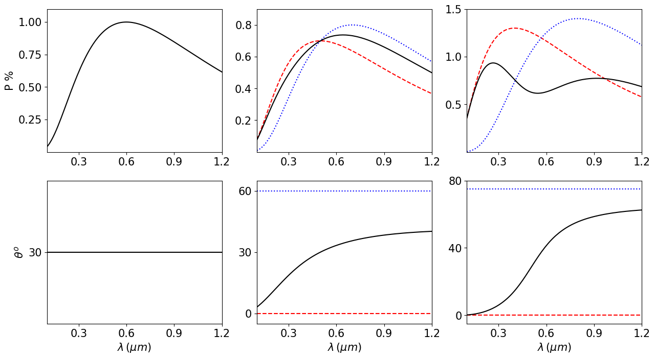
Figure 1: Demonstration of the effect of 3D structure in the Serkowski realtion, using analytical models for $P-\lambda$ and $\theta-\lambda$ curves. In each case, the solid black curve corresponds to the combined model and the dashed red and dotted blue lines corresponds to individual clouds. Left column: The simple case of 1 cloud (Eq. 1). Middle column: An example with 2 Clouds in the LOS, where the combined $P-\lambda$ seems to follow the Serkowski relation, but $\theta-\lambda$ not. Right column: An example with 2 Clouds in the LOS where both $P-\lambda$ and $\theta-\lambda$ profiles deviate from Serkowski expectations. The parameters for each model are: Left: $P_{max}=1\%$, $\lambda_{max}=0.6\mu m$, $\theta=30^{o}$. Middle: $P_{max_{1}}=0.7\%$, $\lambda_{max_{1}}=0.5\mu m$, $\theta_{1}=0^{o}$, $P_{max_{2}}=0.8\%$, $\lambda_{max_{2}}=0.7\mu m$, $\theta_{2}=60^{o}$. Right: $P_{max_{1}}=1.3\%$, $\lambda_{max_{1}}=0.4\mu m$, $\theta_{1}=0^{o}$, $P_{max_{2}}=1.4\%$, $\lambda_{max_{2}}=0.8\mu m$, $\theta_{2}=75^{o}$. For all clouds we have used $K=1.68\cdot\lambda_{max}$ (Wilking et al., 1980).

Modest LOS variations in $\lambda_{max}$ can result in even more complications. In our assumed case of two clouds, a $40\%$ difference in $\lambda_{max}$ between the two clouds leads to nearly identical to the Serkowski curve profiles (middle panel in Fig. 1), although the cumulative signal by construction consists of two underlying profiles. In this case, erroneously assuming a single cloud along the LOS would lead to inaccurate constraints for the parameters of the Serkowski relation, and hence for the grain properties. Significant differences in the EVPAs of two clouds lying along the LOS, such as the one in the employed models which is close to $80$ degrees, can be revealed through the variation of the EVPA as a function of $\lambda$ (bottom middle and right panels in Fig. 1). However, obtaining a sufficient number of data points that would allow us to probe such variations is challenging, and for this reason these data are sparse.

These analytic calculations pose a challenge in the interpretation of $P(\lambda)$ observations: while the Serkowski relation would still hold for individual clouds, the majority of the results extracted from multi-band polarization is likely contaminated by the 3D structure of the ISM, leading to inaccurate dust-grain constraints. The upside of this problem is that it opens up new possibilities for studying the magnetized ISM in 3D.

3 Methods

3.1 Polarimetric data selection – Statistical sample

A recent agglomeration of multi-band optical polarization data (Panopoulou et al., 2023), which is the largest to date, allows us, for the first time, to study in a statistical fashion the impact of the 3D ISM structure of the Galaxy on the Serkowski relation, and the consequences for magnetic field and dust physics studies. In order to fit multiple-cloud models to polarization data it is optimal to use polarization measurements across a broad optical wavelength range. However, for most stars in the literature, measurements exist only in a single or in few bands. Even so, it is possible to evaluate the validity of the Serkowski relation in a statistical manner, by studying an ensemble of sources. We designed such an experiment to test whether stars in single-cloud LOSs are better fit by the Serkowski relation than stars in multiple-cloud LOSs. For acquisition of archival optical polarization measurements for the statistical comparison, we explored Table 6 of the compiled polarization catalog of Panopoulou et al. (2023), which provides polarimetry and distances from Gaia EDR3 (Bailer-Jones et al., 2021) for $\sim 42,000$ sources. We excluded stars with distance greater than 1.25 kpc, as this is the limit of our dust map (see Sect. 3.2). As distance, we take the average of the values (‘r_med_geo’,‘r_med_photogeo’) provided in the catalog. We excluded measurements in filters with no well-defined effective wavelength ($\lambda_{eff}$), therefore, the excluded filters are “0”, “20”, “23”, “51” which correspond to “No filter or unclear”, “weighted-mean”, 0.735-0.804 $\mu m$, 0.5-0.85 $\mu m$, respectively in the catalog. For targets with multiple measurements in the same filter we used the weighted mean and standard deviation of the $q$ measurements, according to

$$q_{\text{mean}}=\frac{\sum(q_{i}\cdot w_{i})}{\sum w_{i}}\,\,and$$ (4)

$$q_{\text{std}}=\frac{\sum w_{i}(x_{i}-\bar{x})^{2}}{\left(\frac{N-1}{N}\right)\cdot\sum w_{i}},$$ (5)

with $w_{i}=1/\sigma_{qi}^{2}$, and $\sigma_{qi}$ the uncertainty of the measurement in $q$, and similarly for $u$. We excluded measurements with debiased $P/\sigma_{P}<2$. Additionally, we did not consider measurements with polarization uncertainty $\sigma_{P}<0.1\%$ because they are likely underestimated , as the most reliable polarization standards to date (Blinov et al., 2023) are only accurate down to $0.1\%$. After all the cuts, we selected targets that have surviving measurements in at least three bands. We note that we did not impose any cut for intrinsically polarized stars (although the Panopoulou et al. (2023) catalog provides this information), as these targets may have been flagged as intrinsically polarized simply because they do not follow the Serkowski relation. However, the final sample does not contain any star that is flagged as intrinsically polarized. After all the cuts, the final sample contains 223 sources with measurements in at least three optical bands.

3.2 Extinction

We collected extinction data for our target stars from the Edenhofer et al. (2024) dust map. We choose this map, as it provides good angular resolution (14’), as well as, parsec-scale distance resolution. The map is available in two versions, one that extends out to 1.25 kpc from the Sun, and one that extends up to 2 kpc, but uses less data for the dust profile reconstruction. We used the 1.25 kpc version, as it should be more accurate, and we did not want to introduce any additional sources of noise. Extinction values in the Edenhofer et al. (2024) map are expressed in the units used by Zhang et al. (2023), the work upon which the dust map was based. We did not renormalize the extinction values in another units system, as we are not interested in the absolute values, but in variations in the dust distribution along the LOS.

For each of our targets, we examined the cumulative extinction ($E$) vs distance ($D$) profiles by eye, in order to identify the number of significant steps ($N_{C}$) in the profile, which presumably correspond to distinct dust clouds. For targets where more than 3 clouds were identified, or the dust profile was very complex, we set $N_{C}>3$. The number of target stars in each subgroup with different number of identified clouds along the LOS are $\#(N_{C}=1)=49$, $\#(N_{C}=2)=74$, $\#(N_{C}=3)=70$, $\#(N_{C}>3)=30$. The targets that correspond to each $N_{C}$ are distributed over different positions on the sky (Fig. 7).

3.3 Fitting the Serkowski relation

In order to evaluate the performance of the Serkowski relation in our statistical sample, we used an extremely powerful, if unconventional in Serkowski studies, technique: we fit our data in the Stokes parameters space $q-u$, exploiting its power to simultaneously trace changes in the profiles of both the degree of polarization and EVPA. Traditionally, the EVPA is not taken into account while fitting the Serkowski formula, thus part of the information imprinted in the polarization signal is ignored. Although the variability of the EVPA with wavelength has been hypothesized to be connected to the existence of multiple clouds (e.g. McMillan & Tapia, 1977; Whittet, 2015), $q-u$ fitting has never been employed to trace the various components (clouds) contributing to the $P-\lambda$ and $\theta-\lambda$ profiles.

As a first step we converted Eq. 1 to the $q-u$ space, with the introduction of $\theta$ in the model as an additional free parameter. Therefore, our model becomes

$$\hat{q}=P_{max}\cdot\exp\left(-K\cdot\ln^{2}{\frac{\lambda_{max}}{\lambda}}\right)\cdot\cos(2\theta),$$ (6a)

$$\hat{u}=P_{max}\cdot\exp\left(-K\cdot\ln^{2}{\frac{\lambda_{max}}{\lambda}}\right)\cdot\sin(2\theta).$$ (6b)

The quantity we wished to minimize for the fits is

$$m=L_{q}+L_{u}+\frac{L_{q}}{L_{u}}+\frac{L_{u}}{L_{q}}$$ (7)

with

$$L_{q}=\frac{1}{N_{\lambda}}\cdot\sum\left(\frac{q_{i}-\hat{q}_{i}}{\sigma_{q_{i}}}\right)^{2},$$ (8a)

$$L_{u}=\frac{1}{N_{\lambda}}\cdot\sum\left(\frac{u_{i}-\hat{u}_{i}}{\sigma_{u_{i}}}\right)^{2},$$ (8b)

where $N_{\lambda}$ the number of different bands where we had measurements for each target, $q_{i}$, $u_{i}$ the measurement in a given band, $\hat{q_{i}}$, $\hat{u_{i}}$ our model as introduced in Eq. 6a, 6b, and $\sigma_{q_{i}}$, $\sigma_{u_{i}}$ the uncertainties of the measurements in $q$ and $u$ respectively. The terms $L_{q}$ and $L_{u}$ are the reduced $\chi^{2}$ metric for $q$ and $u$ respectively. The terms $L_{q}/L_{u}$ and $L_{u}/L_{q}$ were introduced to ensure a balanced contribution from $L_{q}$ and $L_{u}$. For example, if the objective was to minimize just $L_{q}+L_{u}$, the optimal value $V$ could be achieved with $L_{q}=V$ and $L_{u}=0$, $L_{u}=V$ and $L_{q}=0$, or any combination in between. By introducing $L_{q}/L_{u}$ and $L_{u}/L_{q}$, we penalize the model when it favors solutions where $L_{q}=0$ or $L_{u}=0$, thus promoting a more balanced fit.

For the modelling procedure we used the Optuna package in python (Akiba et al., 2019). Optuna is an automatic hyperparameter optimization software framework, originally developed for machine learning hyperparameter-tuning purposes. However, it can also address general optimization problems through the use of a Bayesian optimization framework. We found it highly effective in multi-parameter optimization with few data points and many parameters, such as the case of the $q-u$ modelling, and more efficient in finding the best solution than traditional algorithms such as Markov-Chain Monte-Carlo (MCMC). We used the default options of Optuna with n_trials = 5000 for our fits. Moreover, we adopted the following priors. For $P_{max}$ we initially assumed a rather loose Gaussian prior distribution with a mean of $3\%$ and standard deviation of $3\%$, and enforced it to be positive. For $\lambda_{max}$ we assumed a gaussian prior distribution with the mean 0.6 $\mu m$ and standard deviation 0.2 $\mu m$, and ensured it was always positive. For $K$ we imposed a Gaussian prior distribution with mean $1.68\cdot\lambda_{max}$ and standard deviation $0.13\cdot\lambda_{max}$ (Wilking et al., 1980), and ensured it was always positive. For $\theta$ we assumed a Gaussian prior distribution with mean the average of the polarization values of measurements in individual bands (derived from the average $q$ and $u$ as in Eq. 4 and converted to $\theta$ using Eq. 3b) and $10^{o}$ standard deviation .

We evaluated the quality of our fits by measuring the $\chi^{2}$ per degree of freedom (DoF):

$$\chi^{2}_{\nu}\equiv\frac{\chi^{2}}{DoF}=\frac{\sum\left(\frac{q_{i}-\hat{q}_{i}}{\sigma_{q_{i}}}\right)^{2}+\sum\left(\frac{u_{i}-\hat{u}_{i}}{\sigma_{u_{i}}}\right)^{2}}{2\cdot N_{\lambda}-\nu},$$ (9)

where $\nu=4$ is the number of free parameters in the model ($P_{max}$, $\lambda_{max}$, $K$, $\theta$). We used $2\cdot N_{\lambda}$ as the number of points in Eq. 9 as we accounted for the measurements in both $q$ and $u$ to perform the simultaneous fits. We note that we cannot use $m$ directly (Eq. 7) to evaluate the fits, as $m$ is not a normalized metric, and thus cannot be used for comparing fits to each other.

3.4 Fitting multiple clouds

In order to fit multiple clouds (as in the examples of Sect. 4.1) we used again the $q-u$ fitting technique, following the same logic discussed in Sect. 3.3. The multiple cloud model is derived from Equations 2 and 6, by adding up the $q$ and $u$ components of the individual clouds.

When trying to determine the correct parameters for a model with two or more clouds, the number of parameters is increased (four parameters per cloud), resulting in a substantial number of possible combinations and a vast parameter space to explore. In such situations, identifying the optimal combination of parameters that minimize the cost function can be challenging. To address this, we employed the following procedure. Initially, instead of directly using Optuna, we utilized an MCMC algorithm to rapidly explore the parameter space. Given that the two clouds are interchangeable, we imposed the condition $\lambda_{max_{1}}>\lambda_{max_{2}}$ to focus the algorithm on a single solution. Subsequently, we visually examined the corner plots of the parameters generated by the MCMC algorithm to establish reasonable constraints for the Optuna algorithm, thereby significantly narrowing the search space. Finally, we ran the fit using Optuna, imposing Gaussian priors on the parameters, based on the mean and the spread of the parameters identified by the MCMC algorithm. We chose Optuna to derive the final set of parameters for the model, as it directly provides the optimal set of parameters by minimizing Eq. 7. The fits are evaluated with $\chi^{2}_{\nu}$ (Eq. 9).

4 Results

4.1 Two revealing examples

To demonstrate observationally the impact of the LOS variations of $\lambda_{max}$ and EVPA on the Serkowski relation, we employed archival spectropolarimetric data (Bagnulo et al., 2017). We identified two revealing cases, where the multi-wavelength polarization data show clear evidence of the LOS effects.

The LOS toward the main sequence star HD93222 with spectral type O7 represents a prominent example of what the $P-\lambda$, and $\theta-\lambda$ profiles look like when 3D effects are significant. Firstly, we observe that the $P-\lambda$ deviates from the typical Serkowski curve (Fig. 2 middle panel). Fitting the $P-\lambda$ data with the Serkowski relation requires unphysical values for both $\lambda_{max}$, and $K$ (Table 1), which still yield a merely adequate fit. In addition, $\theta$ varies smoothly with wavelength $\lambda$, which is unexpected when the polarization is dominated by a single cloud with a well defined mean magnetic field. Thus, both $P$ and EVPA show an atypical behaviour with $\lambda$ for this star. Using 3D dust extinction maps (Edenhofer et al., 2024), we verified the existence of multiple clouds along the LOS toward the HD93222 star. The clouds are identified as abrupt increments in extinction as a function of distance (left panel in Fig. 2). The average extinction profile shows three prominent clouds located at around 0.25, 1.35 and 1.8 kpc. The target star, whose estimated distance is 2.44 kpc (Bailer-Jones et al., 2021), lies beyond these clouds, hence its polarization signal carries information from all of them. We fit the data with models with different number of clouds. Although the extinction profile exhibits three distinct steps, the data can be described equally well with both a 2- and a 3-cloud model. This may indicate that two out of three clouds have similar properties. We proceed with the simplest case of a 2-cloud model.

	$P_{\max}$ %	$\lambda_{\max}$ ($\mu m$)	$K$	$\theta$ (∘)	$K/\lambda_{max}$ ($\mu m^{-1}$)	$\chi^{2}_{\nu}$
HD93222
$p-\lambda$ only (This work)	1.42	0.048	0.12	–	2.5	3.33
1-Cloud $q-u$ Model	0.78	0.437	2.55	$-46.80$	5.84	91.49
2-Cloud $q-u$ Model	–	–	–	–	–	2.21
2-Cloud Model - Cloud 1	1.09	0.521	0.96	$-59.15$	1.84	–
2-Cloud Model - Cloud 2	1.11	0.975	1.90	14.49	1.95	–
HD163181
$p-\lambda$ only (Bagnulo et al., 2017)	1.45	0.458	0.50	–	1.09	1.68
1-Cloud $q-u$ Model	1.45	0.496	0.55	$-4.15$	1.11	20.42
2-Cloud $q-u$ Model	–	–	–	–	–	2.46
2-Cloud Model - Cloud 1	1.39	0.463	0.71	$-19.57$	1.53	–
2-Cloud Model - Cloud 2	0.77	0.731	1.00	29.30	1.37	–

Table 1: Fitted parameters for the stars HD163181 and HD93222 in Sect. 4.1.

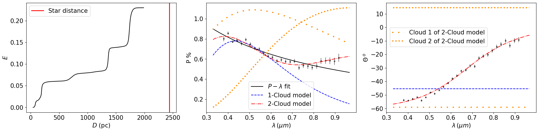
Figure 2: Example of a case where both the $P-\lambda$ and the $\theta-\lambda$ profiles deviate from Serkowski expectations. We are able to fit both profiles by introducing a 2-Cloud model. Data from Bagnulo et al. (2017) for HD93222. Left: Extinction vs distance profile taken from the 2kpc version of the map by Edenhofer et al. (2024). The vertical red line corresponds to the distance of the source. Middle: Data in the $P-\lambda$ space, together with three fitted models: Solid black line: Fit using Eq. 1 in $P-\lambda$ space only. Dashed blue line: Best-fit 1-Cloud model in the $q-u$ space (Eq. 6). Dashed-dotted red line: Best-fit 2-Cloud model in the $q-u$ space (Eq. 6). Dotted orange lines correspond to the two individual components of the 2-Cloud model. Right: Data in $\theta-\lambda$ space together with the three models and the individual components of the 2-Cloud model. Parameters of the fits are quoted in Table 1.

As a second example, we show results for the star HD163181, which is an intermediate-size luminous supergiant of spectral class O9.5 (Fig. 3). In this case, the observed degree of polarization follows the Serkowski formula, but the EVPA varies with wavelength. The 3D extinction profile has two significant steps, hence indicating the existence of more than one dominant clouds along this LOS. Assuming the standard Serkowski curve with a single dominant cloud can yield good fits to the data in the $P-\lambda$ space (Bagnulo et al., 2017), but it fails to explain the observed variability of the EVPA; we verified this by fitting a one cloud model in the $q-u$ plane (dashed blue line in Fig. 3). However, when we considered two clouds along this LOS, as the 3D extinction map suggest, we were able to capture the observed variability of both $P$ and $\theta$ with wavelength (red dashed dotted line in Fig. 3 middle panel).

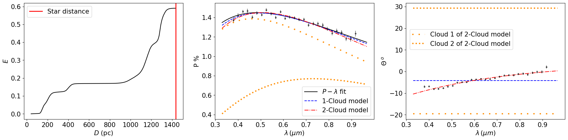
Figure 3: Example of a case where the $P-\lambda$ profile follows the Serkowski relation, but the EVPA does not. By employing a model with two components in the LOS, it is possible to fit both $P$ and $\theta$. Data from Bagnulo et al. (2017) for HD163181. Panels and lines similar to Fig. 2. Parameters of the fits are quoted in Table 1

.

4.2 Statistical sample

We grouped the sample of sources found in Sect. 3.1 into subsamples depending on the number of clouds ($N_{C}$) lying in their LOS, as derived from the 3D extinction map. We obtained four main subsamples: targets in LOSs with one dominant cloud, $N_{C}=1$; with two clouds, $N_{C}=2$; three clouds $N_{C}=3$; and with more than three clouds, $N_{C}>3$. We evaluated the performance of the Serkowski relation in all of the targets as described in Sect. 3.3. We constructed the cumulative density functions (CDFs) of $\chi^{2}_{\nu}$ for the different subsamples (Fig. 4), and we applied the Kolmogorov-Smirnov (KS) test to identify any statistical discrepancies between the $\chi^{2}_{\nu}$ distributions of the $N_{C}=1$ subset and the other three subsets.

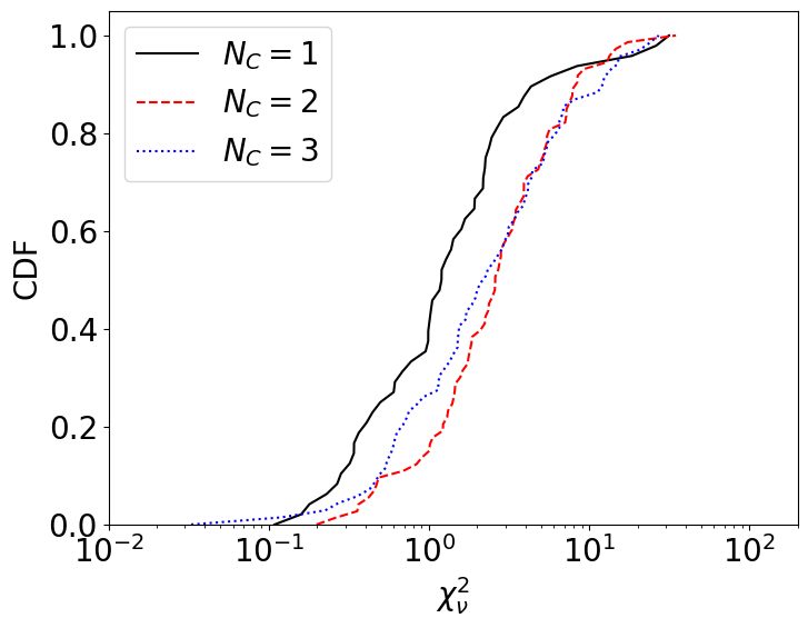
(a)

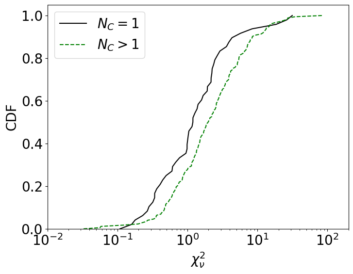
(b)

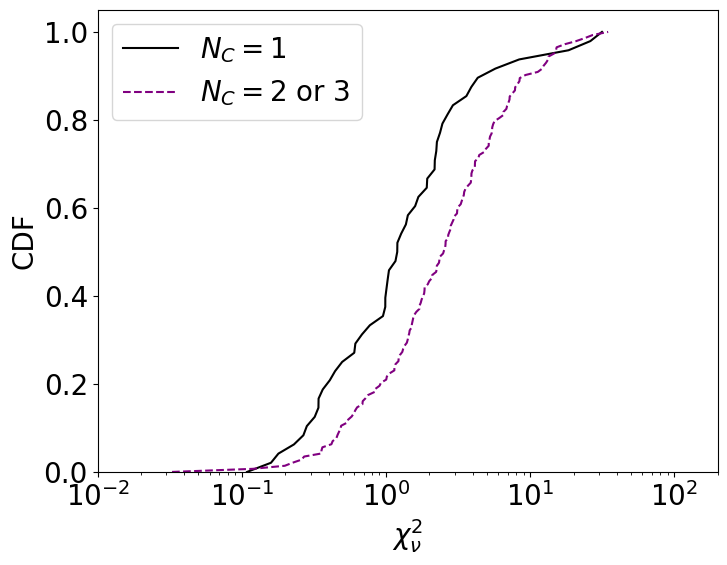
(c)

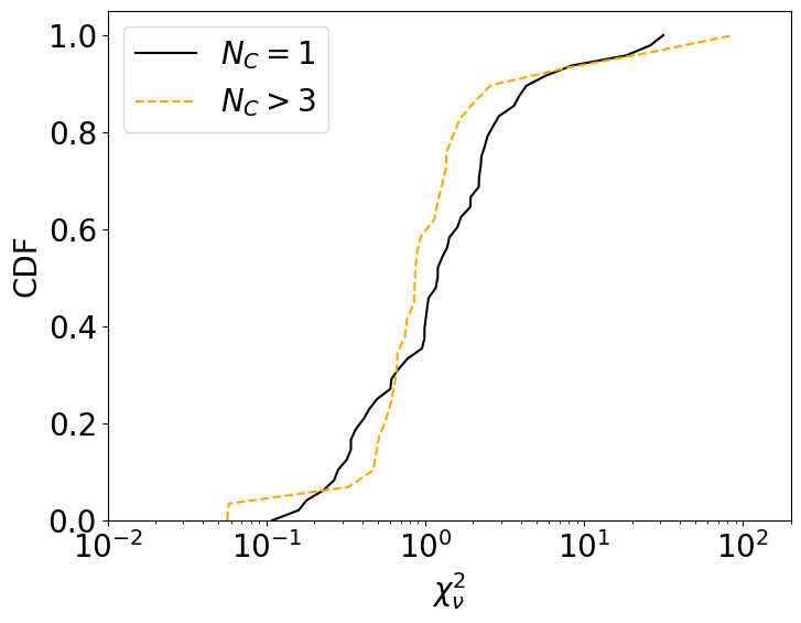
(d)

Figure 4: CDFs of $\chi^{2}_{\nu}$ for different subsamples as described in each label.

We found that the $\chi^{2}_{\nu}$ distribution of the $N_{C}=1$ subset is significantly different from those of subsets with $N_{C}=2$ or $N_{C}=3$. On the contrary, the $\chi^{2}_{\nu}$ distributions of the $N_{C}=1$ subset and of the $N_{C}>3$ subset are not discrepant. The $p-$values of the KS tests for all comparisons are quoted in Table 2, along with the median $\chi^{2}_{\nu}$ for the fits of each subsample. Despite the sparse nature of the data (measurements in only $\sim 3.5$ different filters on average per target) the sample is sufficiently large to allow the statistical distinction of LOSs with two or three clouds from those with only a single cloud. The deterioration of the Serkowski fits in the multi-cloud LOSs is mainly driven by the behaviour of the EVPA with wavelength, and is made clear thanks to our $q-u$ space fits. In contrast, if we perform the fits only on $P-\lambda$, it is not possible to discriminate between LOSs with and without multiple clouds with current data. When the structure in the LOS is too complicated ($N_{C}>3$), there is no statistical difference in the polarization profiles compared to the single cloud case. This is not surprising, as with an increasing number of clouds the variations induced by individual screens tend to average out. Even deviations in the EVPA, which should be more prominent, would become smeared and difficult to detect, especially with limited data points across the spectrum.

Table 2: $p$ - values of the KS test between the subsample of targets with $N_{C}=1$ and other subsamples. See Sect. 4.2 for details.

Subsamples	$p$-value	Median $\chi^{2}_{\nu}$
$N_{C}=1$	1	1.20
$N_{C}=2$	1.5 $\cdot 10^{-3}$	2.59
$N_{C}=3$	2.1 $\cdot 10^{-2}$	2.17
$N_{C}=2$ or 3	$1.8\cdot 10^{-3}$	2.51
$N_{C}>1$	2.1 $\cdot 10^{-2}$	1.97
$N_{C}>3$	$1.5\cdot 10^{-1}$	0.86

4.3 On the parameters of the Serkowski formula

Here we demonstrate how the derived parameters of the Serkowski relation can be incorrect, when erroneously assuming a single cloud in the LOS. We explored how 3D effects affect the distributions of $\lambda_{max}$, and $P_{max}$ that one obtains through the classical fitting of the Serkowski relation in the $P-\lambda$ space; $K$ linearly correlates with $\lambda_{max}$ (Wilking et al., 1980), and thus can be omitted from this analysis. We fit the data only in $P-\lambda$ space (Eq. 1) by minimizing

$$\frac{1}{N_{\lambda}}\cdot\sum\left(\frac{P_{i}-\hat{P_{i}}}{\sigma_{p_{i}}}\right)^{2},$$ (10)

assuming a one-cloud model, and imposing the same priors as discussed in Sect. 3.3. Since the effect of the 3D dust structure is more prominent in $\theta-\lambda$ space, fits in $P-\lambda$ were comparably good for all four subsamples. We then explored the normalized distributions of the derived parameters for all subsamples (Fig. 5 for $\lambda_{max}$, Fig. 6 for $P_{max}$).

Past studies of the Serkowski parameters show that the distribution of $\lambda_{max}$ is singly-peaked, with an average value close to 0.5 $\mu$m (Martin & Whittet, 1990). In contrast, we find that for $N_{C}=1$ (single-cloud sightlines) the intrinsic distribution of $\lambda_{max}$ is bimodal, with peaks at approximately 0.28 and 0.62 $\mu$m. On the other hand, all distributions with $N_{C}>1$ (multiple-cloud sightlines) are unimodal and peak at around 0.55 $\mu$m, which is close to the value that is considered as the Galactic average. By performing Monte Carlo (MC) simulations we found that the unimodality in the $\lambda_{max}$ distribution, which is observed for $N_{C}>1$, can be reproduced with multiple-cloud models with values of $\lambda_{max}$ randomly drawn from the $N_{C}=1$ distribution. The intrinsic Galactic distribution of $\lambda_{max}$ may thus be bimodal, and the currently accepted value for the Galactic average of $\lambda_{max}$ ($\sim 0.5\mu$m) is likely contaminated by LOS effects. Notably, the larger spread of the distribution of $\lambda_{max}$ for the $N_{C}=2$ case is not surprising. Clarke & Al-Roubaie (1984) had theorized that in the case of two clouds in the LOS, the acquired $\lambda_{max}$ from the Serkowski fit is different from the average $\lambda_{max}$ of the two clouds when the two clouds have different parameters. Most areas containing stars behind a single cloud also contain stars behind multiple clouds. We calculated the average $\lambda_{max}$ for targets in distinct areas on the sky (Fig. 7). In most cases, the average $\lambda_{max}$ differs significantly between subsets (see Table 3) located in the same area. This suggests that using the $\lambda_{max}$ of a star from an area with $N_{C}>1$ as a characteristic value for the LOS dust properties could be misleading.

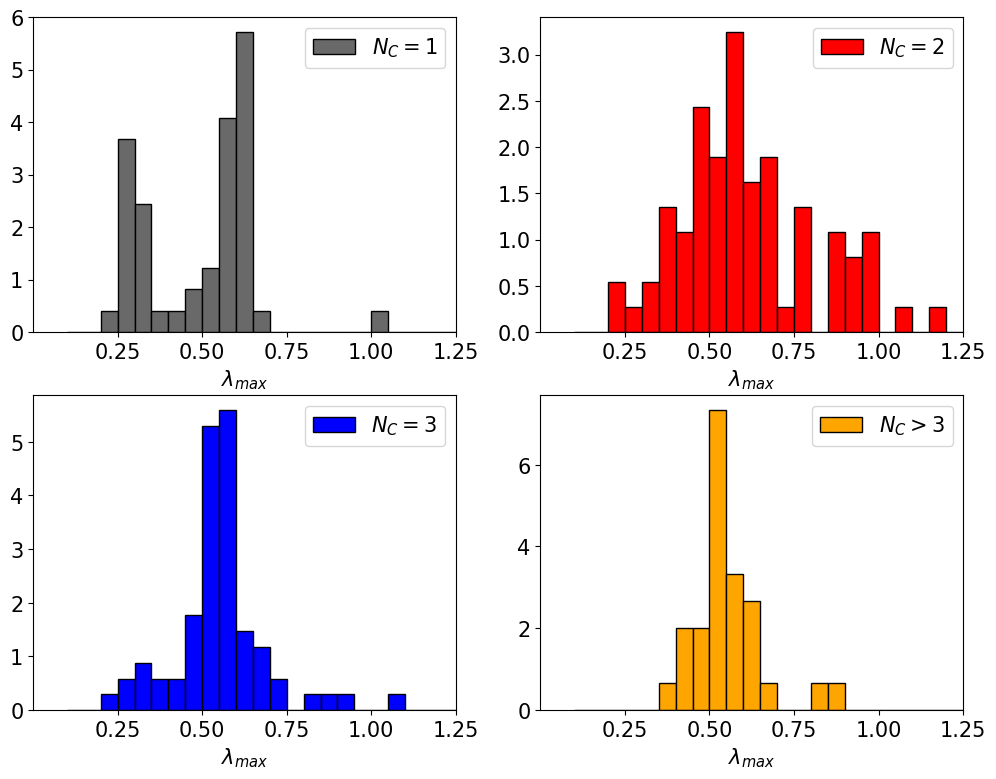
Figure 5: Normalized distributions of $\lambda_{max}$ for subsamples with different number of clouds in the LOS. See Sect. 4.3 for details.

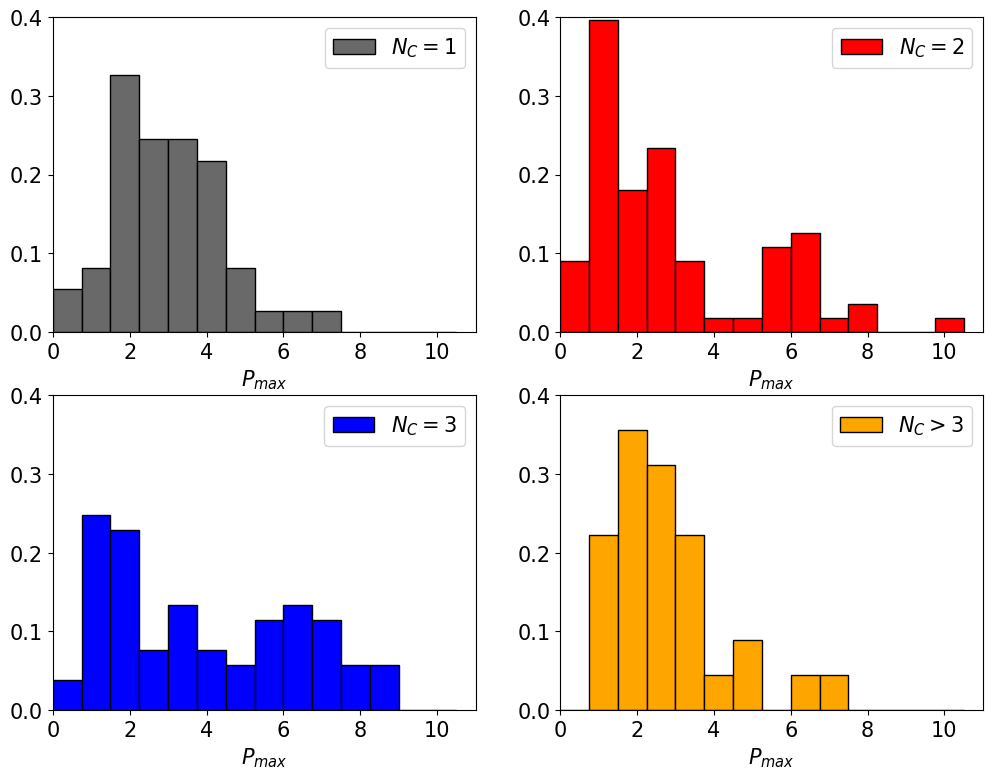
Figure 6: Normalized distributions of $P_{max}$ for subsamples with different number of clouds in the LOS. See Sect. 4.3 for details.

Table 3: Mean $\lambda_{max}$ values in $\mu m$ and their error on the mean for different regions in the sky and different subsamples. Regions with N/A in the error of the mean are cases where there is only one star in the specific region for the subsample.

Region	$N_{C}=1$	$N_{C}=2$	$N_{C}=3$	$N_{C}>3$
A	$0.28\pm 0.02$	$0.56\pm 0.06$
B	$0.34\pm 0.02$		$0.63\pm N/A$
C	$0.83\pm 0.14$	$0.60\pm 0.04$
D	$0.54\pm 0.04$	$0.28\pm N/A$
E	$0.53\pm N/A$	$0.54\pm 0.02$	$0.55\pm 0.02$	$0.55\pm 0.01$
F	$0.52\pm N/A$	$0.52\pm 0.02$	$0.52\pm 0.01$
G	$0.56\pm N/A$			$0.49\pm 0.02$

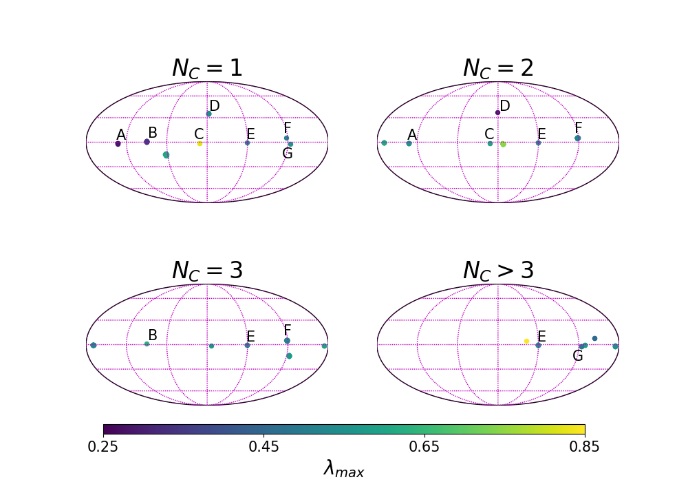
Figure 7: Positions of targets depending on their $N_{C}$. Maps are in Galactic coordinates, in mollweide projection, centered in (0,0). Parallels are drawn every 30^o. Meridians are drawn every 60^o. Longitude increases towards the right-hand side. Colors correspond to the average $\lambda_{max}$ of each area. Marked areas with ’A’ through ’G’ contain stars that are located behind a single as well as multiple clouds. See discussion in Sect. 4.3.

The distribution of $P_{max}$ is also affected by the number of clouds along the LOS. We can immediately see this by assuming, without loss of generality, that two clouds lie along a LOS. The polarization induced by the two clouds can either (partially or totally) add up, or (partially or totally) cancel out, depending on the difference between the EVPAs each would impart on its own.When the EVPA difference is close to 0^o the polarization adds up, while when the difference is close to 90^o it cancels out. This is exactly what we observe in the distributions of $P_{max}$ (Fig. 6). The $P_{max}$ distribution for $N_{C}=1$ is free from LOS effects, hence it should resemble the ”ground truth”. This distribution is unimodal and peaks at $\sim 2.5\%$. On the other hand, the $N_{C}=2$ distribution is bimodal, with both peaks systematically offset from the mode of the $N_{C}=1$ distribution. The bimodality of the $N_{C}=2$ distribution can be understood by the LOS integration effects acting constructively (generating the high-$P_{max}$ peak), or destructively (generating the low-$P_{max}$ peak). The distribution for $N_{C}=3$ displays similar peaks, though it is smoother, as the addition of a third cloud facilitates producing polarization closer to the average observed in the $N_{C}=1$ case. Similarly to $N_{C}=1$, the distribution of the $N_{C}>3$ case is unimodal because an increased number of integration components naturally leads to a distribution with a well-defined peak, as a consequence of the central limit theorem. Overall, both the $\lambda_{max}$, and the $P_{max}$ are significantly affected by the 3D structure of the ISM, which, if ignored, can lead to erroneous Serkowski best-fit parameters.

Our results suggest that fitting a single Serkowski relation is invalid in LOSs with multiple clouds. There can be cases where a single Serkowski relation yields good fits, even when 3D effects are important (Sect. 4.1). However, in these cases the best-fit parameters of a single Serkowski curve are misleading, and not representative of the dust grain physics.

5 Discussion

5.1 Implications for dust modeling

The findings presented in this study have significant implications for dust modeling. Dust models, and grain alignment theories must satisfy the constraints obtained from Serkowski fits (Martin & Whittet, 1990; Andersson et al., 2015; Draine, 2024). However, our results indicate that the Serkowski parameters derived from fitting the observed polarization data in complex interstellar environments may not accurately represent the underlying dust properties, leading to erroneous conclusions about grain size distributions and composition. The results from Sect. 4.3 suggest that the intrinsic distribution of $\lambda_{max}$ in the clouds of our Galaxy may actually be bimodal (Fig. 5). This finding contradicts past studies (Martin & Whittet, 1990), which likely stem from (incorrectly) fitting the Serkowski formula in regions with multiple clouds. Although, our employed sample is the largest to-date, the statistics are still limited, and more data are required to further explore the intrinsic distribution of $\lambda_{max}$ in our Galaxy.

We propose the following two options for constraining the populations of dust in different ISM environments: 1) fit the Serkowski formula only to targets behind a single cloud, or 2) decompose the cumulative polarization signal into its individual components for targets behind multiple clouds to derive the characteristics of each. Moreover, different regions of the Galaxy (e.g., the disk vs. the halo, or varying distances from the Galactic center) may exhibit distinct dust physics that we are currently missing due to the misapplication of the Serkowski relation. By studying the polarization of targets behind multiple clouds and decomposing the signal to derive individual parameters, it may become possible to uncover dust clouds with diverse and potentially novel properties in different parts of the Galaxy.

5.2 Implications for the identification of intrinsically polarized stars

It is customary to iterpret deviations from the Serkowski relation in the $P(\lambda)$ behavior of point sources as indicative of intrinsic polarization mechanisms, such as the presence of circumstellar disks (e.g. Topasna et al., 2023). However, the wavelength dependence of polarization in such cases is known to lack a typical pattern (Bastien, 2015). In contrast, we have demonstrated that fitting simple two-cloud models can account for deviations from the Serkowski formula quite effectively (Sect. 4.1). This suggests that deviations from the Serkowski curve alone are insufficient to indicate the presence of an intrinsic polarization component. In order to validate that a star not following the Serkowski formula is indeed intrinsically polarized, polarization data could be combined with other evidence, such as detection of significant variability, or comparison with neighboring stars.

5.3 The possibility of 3D tomography with the Serkowski relation

Fitting multiple-cloud models to multiwavelength (optical to near-infrared) polarization data paves the way to constraining the LOS variations of the plane-of-the-sky magnetic field morphology (tomography). If the number of clouds in the LOS is known, for instance from 3D extinction maps (e.g., Edenhofer et al., 2024; Green et al., 2019), it is possible to extract the parameters of each individual cloud using the techniques discussed in Sect. 3.4. However, the following considerations should be kept in mind. Firstly, it is possible that two or more clouds in the LOS have similar parameters. In such cases, the polarization data may be adequately fit with fewer clouds than what the 3D extinction maps suggest. For example, if two clouds along a LOS have comparable $\lambda_{max}$ and $\theta$, their polarization contributions will combine, resulting in a profile resembling that of a single cloud but with an increased degree of polarization. This might explain our target star HD93222 (Sect. 4.1), where the extinction profile displays at least three distinct steps, yet the data are sufficiently well-fit by a 2-Cloud model. Another possibility is that the third cloud has a low abundance of aligned grains.

Another strategy one could follow to identify cases of clouds with comparable properties is to obtain measurements of multiple stars at different distances along the same LOS. The polarization signal would vary with distance, as each star would only be influenced by the foreground dust column. Thus, stars lying behind the same clouds would show similar polarization trends, while distinct changes would only occur for stars behind different clouds. Following such methods could complement the BISP-1 algorithm (Pelgrims et al., 2023), which employs single-band optical polarization data with parallaxes from Gaia, for performing ISM tomography along many LOSs (Pelgrims et al., 2024) in the context of optopolarimetric surveys, such as the Pasiphae survey (Tassis et al., 2018). Thus, multiwavelength polarization data promises to provide an independent method for performing ISM magnetic field tomography, which could usher in the era of high-precision 3D magnetized ISM cartography.

6 Summary and Conclusions

In this paper, we showcase the effect of the 3D structure of the ISM on the well-known and widely-used Serkowski relation. Our findings are summarized as follows.

1. We revisited theoretically how the Serkowski formula could become invalid in LOSs with many dust components. We showed that the variations of both the degree of polarization and EVPA with wavelength can be severely affected in some stars. In other stars, the polarization profile may misleadingly appear to follow the Serkowski relation, despite the contribution from multiple dust clouds. In such cases, the imprint of the 3D structure can be mainly observed in the $\theta-\lambda$ profile.

2. As a test case, we selected two different targets that appear to be behind multiple dust clouds, based on their extinction profiles, and for which archival spectropolarimetric data exist. We demonstrated that the single-cloud model, implicitly assumed for Serkowski fits, fails in these cases, while we successfully fitted 2-cloud models.

3. We proposed the $q-u$ fitting technique as the most appropriate approach to fit the Serkowski relation. This method allows for tracing both $P$ and $\theta$ as functions of wavelength simultaneously, enabling fitting for more than one clouds along the LOS.

4. We used a sample of 223 stars behind different number of clouds with polarimetric measurements in three or more bands, to fit and evaluate statistically the performance of the Serkowski formula. We found that the Serkowski formula is not a good model for LOSs with two or more clouds, while it fits well the data in the cases of one or more than three clouds in the LOS. The latter is an outcome of averaging.

5. Our analysis of the fitted parameters of the 223 stars suggests that the intrinsic distribution of the $\lambda_{max}$ parameter in our Galaxy may be bimodal, something that was veiled until now, due to treating sightlines with many clouds as a single dust component.

6. A poor Serkowski fit by itself does not constitute conclusive evidence of intrinsic polarization in a source.

7. Fitting the Serkowski formula for stars behind multiple dust clouds leads to an incorrect estimation of the fitted parameters, and, thus, of the underlying dust physics.

8. Our results hint towards the possibility of performing magnetic tomography using multiband polarization data in combination with Gaia distances.

In conclusion, the Serkowski relation should be cautiously applied when the ISM 3D structure is complex.