[1]Tong-Zhi Yang

Leading Twist-Two Gauge-Variant Counterterms

Thomas Gehrmann    Andreas von Manteuffel   
Abstract

Anomalous dimensions of twist-two operators govern the scale evolution of parton distribution functions. For off-shell external states, the physical twist-two operators mix with unknown gauge-variant operators under renormalization. In this talk, we apply the method proposed by us in [1] to compute all gauge-variant one-loop counterterm Feynman rules with five legs, which enter the determination of the four-loop splitting functions in QCD.

1 Introduction

QCD predictions for high-energy hadron-collider observables rely on the factorization theorem, which encodes the hadron structure in terms of universal parton distribution functions (PDFs). The scale evolution of PDFs, described in the DGLAP evolution equations [2, 3, 4], is governed by splitting functions. Achieving high precision in the determination of PDFs and splitting functions is very desirable for phenomenological applications. The current state-of-the-art calculation for splitting functions extends to the four-loop order, with numerous partial results becoming available recently [5, 6, 7, 8, 9, 10, 11, 12, 13, 14, 15, 16, 17]. These results have already been employed to derive approximate N3LO PDFs [18, 19].

The majority of partial results for four-loop splitting functions (for fixed Mellin moments or specific colour structures) are extracted from the computation of off-shell operator matrix elements (OMEs) to four-loop order. These OMEs are defined as the off-shell matrix elements with a single twist-two quark or gluon operator insertion, and this approach has proven to be computationally efficient in deriving splitting functions. However, under renormalization, the physical twist-two operators mix with unknown gauge-variant (GV) operators. Besides performing the reductions of four-loop integrals for off-shell OMEs with physical twist-two operator insertions, it is the identification of these unknown GV operators or alternatively the determination of the corresponding counterterm Feynman rules that still represents a major challenge in the calculation of the four-loop splitting function. In the past, there have been substantial efforts in this area [20, 21, 22, 23, 24, 25], but a complete solution remained elusive. Generalized BRST and anti-BRST constraints on the form of GV operators at arbitrary $n$ were recently derived in [26]. A method to solve these constraints to compute the corresponding Feynman rules (at leading order) for up to five legs with all-$n$ dependence was subsequently presented in [27]. In [1], we introduced an alternative method that enables the determination of GV counterterm Feynman rules with all-$n$ dependence. This method has been successfully applied to renormalize physical twist-two operators up to three-loop order [1] in a covariant gauge and to extract the $N_{f}^{2}$ contributions [9] to the four-loop pure-singlet splitting functions. In this talk, we further apply this method to derive all leading GV counterterm Feynman rules for five external legs, which constitute a key ingredient to the derivation of the full four-loop splitting functions.

In Section 2, we provide a brief review of the method described in [1]. Section 3 details the derivations of the leading GV counterterm Feynman rules with five legs. Our results are presented in Section 4. Finally, we conclude in Section 5.

2 Review of the method for deriving the GV counterterm Feynman rules

We focus on the renormalization of the physical twist-two operators in the flavor-singlet sector, specifically

$\displaystyle O_{q}(n)$ $\displaystyle=\frac{i^{n-1}}{2}\bigg{[}\bar{\psi}_{i_{1}}\Delta\cdot\gamma(\Delta\cdot D)_{i_{1}i_{2}}(\Delta\cdot D)_{i_{2}i_{3}}\cdots(\Delta\cdot D)_{i_{n-1}i_{n}}\psi_{i_{n}}\bigg{]}\,,$
$\displaystyle O_{g}(n)$ $\displaystyle=-\frac{i^{n-2}}{2}\bigg{[}\Delta_{\mu_{1}}G^{\mu_{1}}_{a_{1}\mu}(\Delta\cdot D)_{a_{1}a_{2}}\cdots(\Delta\cdot D)_{a_{n-2}a_{n-1}}\Delta_{\mu_{n}}G^{\mu_{n}\mu}_{a_{n-1}a_{n}}\bigg{]}\,.$ (1)

where $n$ denotes the Mellin moment (spin) of the operators and $\Delta$ is a light-like reference vector with $\Delta^{2}=0$. As usual, the symbol $\psi$ represents the quark field and $G$ denotes the gluon field strength tensor. The covariant derivative is given by $D^{\mu}=\partial_{\mu}\,\delta-ig_{s}\boldsymbol{T}{}^{a}A^{a}_{\mu}$, where $\boldsymbol{T}{}^{a}$ are the generators of the gauge group and $A^{a}_{\mu}$ is the gauge field. As explained in [1, 28], a naive renormalization

$\displaystyle\left(\begin{array}[]{c}O_{q}\\ O_{g}\end{array}\right)^{\text{R,naive}}=\left(\begin{array}[]{cc}Z_{qq}&Z_{qg}\\ Z_{gq}&Z_{gg}\end{array}\right)\left(\begin{array}[]{c}O_{q}\\ O_{g}\end{array}\right)^{\text{B}}\,$ (8)

is not enough to renormalize the physical twist-two operators beyond one-loop order. Instead, the renormalization should be extended to the following form:

$\displaystyle\left(\begin{array}[]{c}O_{q}\\ O_{g}\\ O_{ABC}\\ \end{array}\right)^{\text{R}}=\left(\begin{array}[]{ccc}Z_{qq}&Z_{qg}&Z_{qA}\\ Z_{gq}&Z_{gg}&Z_{gA}\\ 0&0&Z_{AA}\\ \end{array}\right)\left(\begin{array}[]{c}O_{q}\\ O_{g}\\ O_{ABC}\\ \end{array}\right)^{\text{B}}+\left(\begin{array}[]{c}\left[ZO\right]_{q}^{\textrm{GV}}\\ \left[ZO\right]_{g}^{\textrm{GV}}\\ \left[ZO\right]_{A}^{\textrm{GV}}\end{array}\right)^{\text{B}},$ (21)

where we use the shorthand notation $O_{ABC}=O_{A}+O_{B}+O_{C}$, with $O_{A},\,O_{B},\,O_{C}$ denoting the leading GV twist-two operators involving all-gluon, quark-gluon, and ghost-gluon fields, respectively. At higher orders of the strong coupling, three GV counterterms denoted as $\left[ZO\right]_{q}^{\textrm{GV}},\left[ZO\right]_{g}^{\textrm{GV}},\left[ZO\right]_{A}^{\textrm{GV}}$ are required in addition to renormalize the physical operators. For the GV counterterms, $Z$ and $O$ are combined as $\left[ZO\right]$ since it is in general not possible (and also not required in practice) to separate the renormalization constants $Z$ from their associated operators $O$ when retaining the all-$n$ dependence in our approach.

One can formally expand the GV counterterms in the following form:

$\displaystyle\left[ZO\right]_{i}^{\textrm{GV}}=\sum_{l=2}^{\infty}a_{s}^{l}\left[ZO\right]_{i}^{\textrm{GV},\,\left(l\right)},\text{with }i=q,g,A\,,$ (22)

with $a_{s}=\alpha_{s}/(4\pi)$. The contributions from GV operators or counterterms start at different orders of $a_{s}$,

$\displaystyle Z_{qA}=\mathcal{O}(a_{s}^{2}),\quad Z_{gA}=$ $\displaystyle\mathcal{O}(a_{s}),\quad\left[ZO\right]_{q}^{\textrm{GV}}=\mathcal{O}(a_{s}^{3}),\quad\left[ZO\right]_{g}^{\textrm{GV}}=\mathcal{O}(a_{s}^{2}),$
$\displaystyle Z_{AA}=\mathcal{O}(a_{s}^{0}),\quad\left[ZO\right]_{A}^{\textrm{GV}}=\mathcal{O}(a_{s})\,.$ (23)

An interesting observation in [1] is that the (counterterm) Feynman rules for the corresponding GV operators can be extracted by inserting eq. (21) into matrix elements with more than two off-shell external states, even without knowing the operators themselves. Without loss of generality, we will consider the renormalization of the physical gluon operator:

$\displaystyle O^{\text{R}}_{g}=Z_{gq}O^{\text{B}}_{q}+Z_{gg}O^{\text{B}}_{g}+Z_{gA}O_{ABC}^{\text{B}}+\left[ZO\right]_{g}^{\textrm{GV}}\,.$ (24)

Since we are discussing the renormalization of a leading-twist operator, it suffices to consider one-particle-irreducible (1PI) OMEs with all-off-shell external states composed of two particles of type $j$ plus $m$ gluons,

$\displaystyle\braket{j}{O_{g}}{j+m\,g}^{\mu_{1}\cdots\mu_{m},\,\text{R}}_{\text{1PI}}=Z_{j}(\sqrt{Z_{g}})^{m}\bigg{[}\braket{j}{(Z_{gq}O_{q}+Z_{gg}O_{g})}{j+m\,g}^{\mu_{1}\cdots\mu_{m},\,\text{B}}_{\text{1PI}}\bigg{]}$
$\displaystyle\qquad+Z_{j}(\sqrt{Z_{g}})^{m}\bigg{[}Z_{gA}\braket{j}{O_{ABC}}{j+m\,g}^{\mu_{1}\cdots\mu_{m},\,\text{B}}_{\text{1PI}}+\braket{j}{\left[ZO\right]_{g}^{\textrm{GV}}}{j+m\,g}^{\mu_{1}\cdots\mu_{m},\,\text{B}}_{\text{1PI}}\bigg{]}\,,$ (25)

where $j$ can be a quark($q$), gluon($g$), or ghost($c$) external state, and $\sqrt{Z_{j}}$ is the corresponding wave function renormalization constant. To continue, we expand the off-shell OMEs according to the number of loops $l$ and legs $m+2$,

$\displaystyle\braket{j}{O}{j+m\,g}^{\mu_{1}\cdots\mu_{m}\text{}}=\sum_{l=0}^{\infty}\left[\braket{j}{O}{j+m\,g}^{\mu_{1}\cdots\mu_{m},\,(l),\,(m)\text{}}_{\text{}}\right]a_{s}^{l}\,g_{s}^{m}\,.$ (26)

Since the left-hand side of equation (2) is ultraviolet-renormalized and infrared finite (with all external states being off-shell), the summation on the right-hand side of the equation must also be free of poles in the dimensional regulator $\epsilon$. This provides a method for deriving the GV (counterterm) Feynman rules by computing the corresponding off-shell OMEs order by order in the strong coupling. As an example, the two-ghost plus $m$-gluon Feynman rules for $O_{C}$ operator can be written in the following compact form,

$\displaystyle{\color[rgb]{0,0,0}{\braket{c}{O_{C}}{c+m\,g}^{\mu_{1}\cdots\mu_{m},\,{\color[rgb]{0,0,0}(0)},\,(m)}_{\text{}}=\frac{-1}{Z_{gA}^{(1)}}\left[\braket{c}{O_{g}}{c+m\,g}^{\mu_{1}\cdots\mu_{m},\,(1),\,(m),\,\text{B}}_{\text{1PI}}\right]_{\text{div}}}}\,.$ (27)

Here the subscript ’div’ is the pole part in $\epsilon$, and $Z_{gA}^{(1)}$ is the leading GV renormalization constant

$$Z_{gA}^{(1)}=\frac{1}{\epsilon}\frac{C_{A}}{n(n-1)}\,.$$ (28)

Note that the above method is general and can be applied to extract (counterterm) Feynman rules to any number of loops and legs. In the following, we focus on the determination of Feynman rules with five legs for the leading GV operators, i.e. operators $O_{A}\,,O_{B}\,,O_{C}$.

3 Computations of five-leg Feynman rules for operators
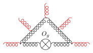
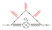
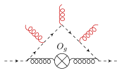
 OA,OB,OCsubscript𝑂𝐴subscript𝑂𝐵subscript𝑂𝐶O_{A},O_{B},O_{C}

To extract Feynman rules for operators $O_{A}\,,O_{B}\,,O_{C}$, we can simply expand the eq. (2) to one-loop order, where the two-loop GV counterterms are absent. In the following, we focus on the case with five legs. Some example Feynman diagrams are shown in Fig. 1.

Refer to caption
Refer to caption
Refer to caption
Figure 1: Sample 1-loop diagrams to determine the Feynman rules with 5 legs stemming from $O_{A},O_{B},O_{C}$ operators respectively. Here, all external states are off-shell, and all diagrams involve the insertion of the physical gluon operator $O_{g}$.

We consider the computations of one-loop all-off-shell five-particle scatterings with an insertion of the operator $O_{g}$, involving 14 scales

$\displaystyle p_{1}^{2},p_{2}^{2},p_{3}^{2},p_{4}^{2},p_{1}\cdot p_{2},p_{1}\cdot p_{3},p_{1}\cdot p_{4},p_{2}\cdot p_{3},p_{2}\cdot p_{4},p_{3}\cdot p_{4},\Delta\cdot p_{1},\Delta\cdot p_{2},\Delta\cdot p_{3},\Delta\cdot p_{4}\,.$ (29)

Here, we eliminated $p_{5}$ by momentum conservation

$\displaystyle\sum_{i=1}^{5}p_{i}=0\,.$ (30)

To retain the all-$n$ dependence for the off-shell OMEs, we employ the generating function method introduced in [29, 30]. This method sums non-standard terms in the Feynman rules, such as $(\Delta\cdot p)^{n-1}$ into linear propagators that depend on a tracing parameter, $t$. For example,

$\displaystyle(\Delta\cdot p)^{n-1}\to\sum_{n=1}^{\infty}(\Delta\cdot p)^{n-1}t^{n}=\frac{t}{1-t\Delta\cdot p}\,.$ (31)

By working in $t$-space, we can perform standard IBP reductions [31, 32] and extract the desired $n$-space results in the final step by expanding the parameter $t$ around $t=0$.

It is highly non-trivial to directly compute the one-loop all-off-shell OMEs with 14 scales. Luckily the computation can be greatly simplified by analyzing the structures of Feynman rules for a twist-two operator. According to the dimensional analysis shown in [1], the Feynman rules for operators $O_{B}$ and $O_{C}$ consist of one Lorentz tensor only

$\displaystyle\left[\braket{c}{O_{C}}{c+m\,g}^{\mu_{1}\cdots\mu_{m},\,(0),\,(m)}_{\text{}}\right]=c_{m}\Delta^{\mu_{1}}\Delta^{\mu_{2}}\cdots\Delta^{\mu_{m}}\,,$
$\displaystyle\left[\braket{q}{O_{B}}{q+m\,g}^{\mu_{1}\cdots\mu_{m},\,(0),\,(m)}_{\text{}}\right]=b_{m}\Delta^{\mu_{1}}\Delta^{\mu_{2}}\cdots\Delta^{\mu_{m}}\,,$ (32)

and the coefficients $c_{m}\,,b_{m}$ are functions of $\Delta\cdot p_{i}$ only. The Feynman rule for operator $O_{A}$ with five legs is composed of 31 tensor structures:

$\displaystyle\left[\braket{g}{O_{A}}{gggg}^{\mu_{1}\mu_{2}\mu_{3}\mu_{4}\mu_{5},\,(0),\,(3)}_{\text{}}\right]=a_{1}\Delta^{\mu_{1}}\Delta^{\mu_{2}}\Delta^{\mu_{3}}\Delta^{\mu_{4}}\Delta^{\mu_{5}}$
$\displaystyle\quad+\Delta^{\mu_{1}}\Delta^{\mu_{2}}\Delta^{\mu_{3}}\Delta^{\mu_{4}}(a_{2}p_{1}^{\mu_{5}}+a_{3}p_{2}^{\mu_{5}}+a_{4}p_{3}^{\mu_{5}}+a_{5}p_{4}^{\mu_{5}})$
$\displaystyle\quad+\Delta^{\mu_{1}}\Delta^{\mu_{2}}\Delta^{\mu_{3}}\Delta^{\mu_{5}}(a_{6}p_{1}^{\mu_{4}}+a_{7}p_{2}^{\mu_{4}}+a_{8}p_{3}^{\mu_{4}}+a_{9}p_{4}^{\mu_{4}})$
$\displaystyle\quad+\Delta^{\mu_{1}}\Delta^{\mu_{2}}\Delta^{\mu_{4}}\Delta^{\mu_{5}}(a_{10}p_{1}^{\mu_{3}}+a_{11}p_{2}^{\mu_{3}}+a_{12}p_{3}^{\mu_{3}}+a_{13}p_{4}^{\mu_{3}})$
$\displaystyle\quad+\Delta^{\mu_{1}}\Delta^{\mu_{3}}\Delta^{\mu_{4}}\Delta^{\mu_{5}}(a_{14}p_{1}^{\mu_{2}}+a_{15}p_{2}^{\mu_{2}}+a_{16}p_{3}^{\mu_{2}}+a_{17}p_{4}^{\mu_{2}})$
$\displaystyle\quad+\Delta^{\mu_{2}}\Delta^{\mu_{3}}\Delta^{\mu_{4}}\Delta^{\mu_{5}}(a_{18}p_{1}^{\mu_{1}}+a_{19}p_{2}^{\mu_{1}}+a_{20}p_{3}^{\mu_{1}}+a_{21}p_{4}^{\mu_{1}})$
$\displaystyle\quad+a_{22}\Delta^{\mu_{1}}\Delta^{\mu_{2}}\Delta^{\mu_{3}}g^{\mu_{4}\mu_{5}}+a_{23}\Delta^{\mu_{1}}\Delta^{\mu_{2}}\Delta^{\mu_{4}}g^{\mu_{3}\mu_{5}}+a_{24}\Delta^{\mu_{1}}\Delta^{\mu_{2}}\Delta^{\mu_{5}}g^{\mu_{3}\mu_{4}}+a_{25}\Delta^{\mu_{1}}\Delta^{\mu_{3}}\Delta^{\mu_{4}}g^{\mu_{2}\mu_{5}}$
$\displaystyle\quad+a_{26}\Delta^{\mu_{1}}\Delta^{\mu_{3}}\Delta^{\mu_{5}}g^{\mu_{2}\mu_{4}}+a_{27}\Delta^{\mu_{1}}\Delta^{\mu_{4}}\Delta^{\mu_{5}}g^{\mu_{2}\mu_{3}}+a_{28}\Delta^{\mu_{2}}\Delta^{\mu_{3}}\Delta^{\mu_{4}}g^{\mu_{1}\mu_{5}}$
$\displaystyle\quad+a_{29}\Delta^{\mu_{2}}\Delta^{\mu_{3}}\Delta^{\mu_{5}}g^{\mu_{1}\mu_{4}}+a_{30}\Delta^{\mu_{2}}\Delta^{\mu_{4}}\Delta^{\mu_{5}}g^{\mu_{1}\mu_{3}}+a_{31}\Delta^{\mu_{3}}\Delta^{\mu_{4}}\Delta^{\mu_{5}}g^{\mu_{1}\mu_{2}}\,,$ (33)

where the coefficient $a_{1}$ is linear in the Mandelstam variables $p_{i}^{2},p_{i}\cdot p_{j}$. Similarly to $c_{m}$ and $d_{m}$ in eq. (3), the coefficients $a_{j}$ for $j\geq 2$ depend solely on $\Delta\cdot p_{i}$.

Owing to these properties, the evaluation of the five-parton one-loop OME and the corresponding IBP reduction can be performed by setting all Mandelstam variables to non-zero rational numbers, which significantly simplifies the workflow. A single numerical sample is sufficient to determine the Feynman rules involving quarks or ghosts, with an additional sample used for cross-checking. In the case of the five-gluon Feynman rules, one numerical sample is also enough to fix the unknown parameters, thanks to the symmetry constraints imposed by Bose statistics.

Another simplification arises from the fact that the Feynman rules are contained in the $\epsilon$-divergent part of the OMEs. Consequently, only the following two types of Feynman integrals contribute:

$\displaystyle I_{1}$ $\displaystyle=(\mu^{2})^{\epsilon}\int\frac{d^{d}l}{i\pi^{d/2}}\frac{1}{(l-q_{1})^{2}l^{2}}\,,$
$\displaystyle I_{2}$ $\displaystyle=(\mu^{2})^{\epsilon}\int\frac{d^{d}l}{i\pi^{d/2}}\frac{1}{(l-q_{1})^{2}l^{2}\big{(}1-t\Delta\cdot(l+q_{2})\big{)}}\,,$ (34)

where $q_{1}\,,\,q_{2}$ are linear combinations of the momenta $p_{1}\,,\,\cdots\,,\,p_{4}$ and $\mu$ is the ’t Hooft mass. These two master integrals can be solved to high orders in $\epsilon$ without much effort. Here, we only need their single-pole terms:

$\displaystyle I_{1}=\frac{1}{\epsilon}+\mathcal{O}(\epsilon^{0})\,,$
$\displaystyle I_{2}=\frac{1}{\epsilon}\left[\frac{\ln(1-t\Delta\cdot q_{1}-t\Delta\cdot q_{2})-\ln(1-t\Delta\cdot q_{2})}{-t\Delta\cdot q_{1}}\right]+\mathcal{O}(\epsilon^{0})\,.$ (35)

With these simplifications, the computational steps follow a standard chain, where several packages are involved, including QGRAF [33], FORM [34], Apart [35], Kira [36], FiniteFlow [37], MultivariateApart [38]. We obtain the $t$-space results for the single-pole contributions in $\epsilon$ of one-loop off-shell OMEs. These results are then transformed back into $n$-space. Next, we perform renormalization to one-loop order according to eq. (2), which provides us with the Feynman rules with five legs for the operators $O_{A},\,O_{B},\,O_{C}$.

4 Results

We are now ready to present the all-$n$ Feynman rules for the $O_{B},\,O_{C},\,O_{A}$ operators with 5 legs. The Feynman rules up to four legs within the same framework can be found in  [1]. Using the convention of all momenta flowing into the vertices, the results read

$\displaystyle\quad\to\frac{-g_{s}^{3}}{4}\frac{1+(-1)^{n}}{2}\not{\Delta}\Delta^{\mu_{3}}\Delta^{\mu_{4}}\Delta^{\mu_{5}}\left(T^{a}\right)_{i_{2}i_{1}}\sum_{j_{1}=0}^{n-4}\sum_{j_{2}=0}^{j_{1}}\bigg{(}\left(\Delta\cdot p_{4}\right){}^{j_{2}}\left(\Delta\cdot\left(p_{4}+p_{5}\right)\right){}^{-j_{1}+n-4}$
$\displaystyle\qquad\times\Big{[}\left(5\text{Tr}(T_{A}^{a}T_{A}^{a_{3}}T_{A}^{a_{5}}T_{A}^{a_{4}})-4\text{Tr}(T_{A}^{a}T_{A}^{a_{3}}T_{A}^{a_{4}}T_{A}^{a_{5}})\right)\left(-\Delta\cdot\left(p_{1}+p_{2}\right)\right){}^{j_{1}-j_{2}}$
$\displaystyle\qquad-\left(\text{Tr}(T_{A}^{a}T_{A}^{a_{3}}T_{A}^{a_{4}}T_{A}^{a_{5}})-2\text{Tr}(T_{A}^{a}T_{A}^{a_{3}}T_{A}^{a_{5}}T_{A}^{a_{4}})\right)\left(-\Delta\cdot p_{3}\right){}^{j_{1}-j_{2}}\Big{]}\bigg{)}$
$\displaystyle\qquad+\text{permutations of three gluons}\,,$ (36)
$\displaystyle\quad\to\Bigg{[}\frac{ig_{s}^{3}}{192}\frac{1+(-1)^{n}}{2}\Delta^{\mu_{3}}\Delta^{\mu_{4}}\Delta^{\mu_{5}}\bigg{\{}\frac{3}{2}\left(f_{11}-2f_{12}\right)\sum_{j_{1}=0}^{n-3}\left(\left(\Delta\cdot p_{4}\right){}^{j_{1}}\left(-\Delta\cdot p_{3}\right){}^{-j_{1}+n-3}\right)$
$\displaystyle\qquad+12f_{8}\sum_{j_{1}=0}^{n-3}\left(\left(\Delta\cdot p_{4}\right){}^{j_{1}}\left(\Delta\cdot\left(-p_{1}-p_{3}\right)\right){}^{-j_{1}+n-3}\right)$
$\displaystyle\qquad+4\left(6f_{2}+13f_{8}+f_{9}\right)\sum_{j_{1}=0}^{n-3}\sum_{j_{2}=0}^{j_{1}}\left(\left(\Delta\cdot\left(p_{1}+p_{3}\right)\right){}^{j_{1}-j_{2}}\left(\Delta\cdot\left(-p_{2}-p_{5}\right)\right){}^{j_{2}}\left(-\Delta\cdot p_{2}\right){}^{-j_{1}+n-3}\right)$
$\displaystyle\qquad+4\left(6f_{2}+4f_{8}+f_{9}\right)\sum_{j_{1}=0}^{n-3}\sum_{j_{2}=0}^{j_{1}}\left(\left(\Delta\cdot p_{4}\right){}^{j_{1}-j_{2}}\left(\Delta\cdot\left(-p_{2}-p_{5}\right)\right){}^{j_{2}}\left(-\Delta\cdot p_{2}\right){}^{-j_{1}+n-3}\right)$
$\displaystyle\qquad-3\left(6f_{2}+6f_{3}+6f_{4}+6f_{5}+6f_{6}+f_{8}-f_{9}-f_{10}\right)$
$\displaystyle\qquad\times\sum_{j_{1}=0}^{n-3}\sum_{j_{2}=0}^{j_{1}}\left(\left(-\Delta\cdot p_{3}\right){}^{j_{1}-j_{2}}\left(\Delta\cdot\left(-p_{3}-p_{5}\right)\right){}^{j_{2}}\left(\Delta\cdot\left(p_{1}+p_{2}\right)\right){}^{-j_{1}+n-3}\right)$
$\displaystyle\qquad+\left(-6f_{1}-14f_{7}+13f_{11}\right)\Delta\cdot(p_{1}-p_{2})$
$\displaystyle\qquad\times\sum_{j_{1}=0}^{n-4}\sum_{j_{2}=0}^{j_{1}}\left(\left(-\Delta\cdot p_{3}\right){}^{j_{1}-j_{2}}\left(-\Delta\cdot\left(p_{3}+p_{5}\right)\right){}^{j_{2}}\left(\Delta\cdot\left(p_{1}+p_{2}\right)\right){}^{-j_{1}+n-4}\right)$
$\displaystyle\qquad-4\left(6f_{2}+f_{8}+4f_{9}\right)\sum_{j_{1}=0}^{n-3}\sum_{j_{2}=0}^{j_{1}}\left(\left(-\Delta\cdot p_{4}\right){}^{j_{2}}\left(\Delta\cdot\left(-p_{4}-p_{5}\right)\right){}^{j_{1}-j_{2}}\left(\Delta\cdot p_{2}\right){}^{-j_{1}+n-3}\right)$
$\displaystyle\qquad+\left(-6f_{1}+f_{7}+4f_{11}\right)\Delta\cdot(p_{1}-p_{2})$
$\displaystyle\qquad\times\sum_{j_{1}=0}^{n-4}\sum_{j_{2}=0}^{j_{1}}\left(\left(-\Delta\cdot\left(p_{3}+p_{4}\right)\right){}^{j_{1}-j_{2}}\left(\Delta\cdot p_{5}\right){}^{j_{2}}\left(-\Delta\cdot p_{3}\right){}^{-j_{1}+n-4}\right)$
$\displaystyle\qquad+18f_{8}\sum_{j_{1}=0}^{n-3}\left(\left(\Delta\cdot\left(p_{2}+p_{5}\right)\right){}^{j_{1}}\left(\Delta\cdot\left(-p_{1}-p_{3}\right)\right){}^{-j_{1}+n-3}\right)$
$\displaystyle\qquad-3e_{1}\sum_{j_{1}=0}^{n-3}\sum_{j_{2}=0}^{j_{1}}\sum_{j_{3}=0}^{j_{2}}\left(\left(\Delta\cdot p_{2}\right){}^{j_{1}-j_{2}}\left(-\Delta\cdot\left(p_{1}+p_{3}\right)\right){}^{j_{2}-j_{3}}\left(\Delta\cdot\left(p_{2}+p_{5}\right)\right){}^{j_{3}}\left(-\Delta\cdot p_{1}\right){}^{-j_{1}+n-3}\right)$
$\displaystyle\qquad-9\left(f_{7}-2f_{9}\right)\sum_{j_{1}=0}^{n-3}\left(\left(\Delta\cdot p_{5}\right){}^{j_{1}}\left(\Delta\cdot\left(p_{4}+p_{5}\right)\right){}^{-j_{1}+n-3}\right)\bigg{\}}+(p_{1}\leftrightarrow p_{2},\,a_{1}\leftrightarrow a_{2})\Bigg{]}$
$\displaystyle\qquad+\text{permutations of three gluons}\,,$ (37)
$\displaystyle\quad\to ig_{s}^{3}\frac{1+(-1)^{n}}{2}\bigg{\{}-\frac{1}{16}\left(2f_{8}-f_{9}\right)\Delta^{\mu_{1}}\Delta^{\mu_{2}}\Delta^{\mu_{3}}g^{\mu_{4}\mu_{5}}\bigg{[}\sum_{j_{1}=0}^{n-3}\left(\left(-\Delta\cdot p_{3}\right){}^{j_{1}}\left(\Delta\cdot p_{1}\right){}^{-j_{1}+n-3}\right)$
$\displaystyle\qquad+6\sum_{j_{1}=0}^{n-3}\left(\left(\Delta\cdot\left(p_{1}+p_{3}\right)\right){}^{j_{1}}\left(\Delta\cdot p_{1}\right){}^{-j_{1}+n-3}\right)\bigg{]}$
$\displaystyle\qquad+\frac{1}{48}\Delta^{\mu_{2}}\Delta^{\mu_{4}}\Delta^{\mu_{5}}\left(2g^{\mu_{1}\mu_{3}}\Delta\cdot p_{1}+\Delta^{\mu_{3}}p_{1}^{\mu_{1}}-4\Delta^{\mu_{1}}p_{1}^{\mu_{3}}\right)$
$\displaystyle\qquad\times\bigg{[}\left(6f_{2}+13f_{8}+f_{9}\right)\sum_{j_{1}=0}^{n-4}\sum_{j_{2}=0}^{j_{1}}\left(\left(\Delta\cdot\left(p_{1}+p_{3}\right)\right){}^{j_{1}-j_{2}}\left(\Delta\cdot\left(-p_{2}-p_{5}\right)\right){}^{j_{2}}\left(-\Delta\cdot p_{2}\right){}^{-j_{1}+n-4}\right)$
$\displaystyle\qquad+\left(6f_{2}+4f_{8}+f_{9}\right)\sum_{j_{1}=0}^{n-4}\sum_{j_{2}=0}^{j_{1}}\left(\left(\Delta\cdot p_{4}\right){}^{j_{1}-j_{2}}\left(\Delta\cdot\left(-p_{2}-p_{5}\right)\right){}^{j_{2}}\left(-\Delta\cdot p_{2}\right){}^{-j_{1}+n-4}\right)\bigg{]}$
$\displaystyle\qquad-\frac{1}{64}e_{1}\Delta^{\mu_{3}}\Delta^{\mu_{4}}\Delta^{\mu_{5}}\left(\Delta^{\mu_{2}}p_{1}^{\mu_{1}}-\Delta^{\mu_{1}}p_{2}^{\mu_{2}}\right)$
$\displaystyle\qquad\times\sum_{j_{1}=0}^{n-4}\sum_{j_{2}=0}^{j_{1}}\sum_{j_{3}=0}^{j_{2}}\left(\left(\Delta\cdot p_{2}\right){}^{j_{1}-j_{2}}\left(\Delta\cdot\left(-p_{1}-p_{3}\right)\right){}^{j_{2}-j_{3}}\left(\Delta\cdot\left(p_{2}+p_{5}\right)\right){}^{j_{3}}\left(-\Delta\cdot p_{1}\right){}^{-j_{1}+n-4}\right)$
$\displaystyle\qquad+\Delta^{\mu_{1}}\Delta^{\mu_{2}}\Delta^{\mu_{3}}\Delta^{\mu_{4}}\Delta^{\mu_{5}}\bigg{[}\left(\frac{1}{192}p_{3}\cdot p_{3}(-3e_{1}-e_{2})+\frac{1}{384}p_{4}\cdot p_{4}(e_{1}+e_{3})-\frac{1}{64}e_{1}p_{1}\cdot p_{1}\right)$
$\displaystyle\qquad\times\sum_{j_{1}=0}^{n-5}\sum_{j_{2}=0}^{j_{1}}\sum_{j_{3}=0}^{j_{2}}\left(\left(\Delta\cdot p_{2}\right){}^{j_{1}-j_{2}}\left(\Delta\cdot\left(-p_{1}-p_{3}\right)\right){}^{j_{2}-j_{3}}\left(\Delta\cdot\left(p_{2}+p_{5}\right)\right){}^{j_{3}}\left(-\Delta\cdot p_{1}\right){}^{-j_{1}+n-5}\right)$
$\displaystyle\qquad+\left(p_{1}\leftrightarrow p_{2},\,p_{3}\leftrightarrow p_{5},\,a_{1}\leftrightarrow a_{2},\,a_{3}\leftrightarrow a_{5}\right)\bigg{]}\bigg{\}}+\text{permutations of five gluons}\,,$ (38)

where we have defined the following linearly independent color structures for operators $O_{A}$ and $O_{C}$:

$\displaystyle f_{1}=d_{4f}^{a_{3}a_{4}a_{5}a_{1}a_{2}},\,f_{2}=d_{4f}^{a_{2}a_{4}a_{5}a_{1}a_{3}},\,f_{3}=d_{4f}^{a_{2}a_{3}a_{4}a_{1}a_{5}},\,$
$\displaystyle f_{4}=d_{4f}^{a_{1}a_{4}a_{5}a_{2}a_{3}},\,f_{5}=d_{4f}^{a_{1}a_{3}a_{4}a_{2}a_{5}},\,f_{6}=d_{4f}^{a_{1}a_{2}a_{4}a_{3}a_{5}},\,$
$\displaystyle f_{7}=f^{aa_{4}a_{5}}\ f^{aba_{3}}\ f^{ba_{1}a_{2}},\,f_{8}=f^{aa_{2}a_{5}}\ f^{aba_{4}}\ f^{ba_{1}a_{3}},\,f_{9}=f^{aa_{4}a_{5}}\ f^{aba_{2}}\ f^{ba_{1}a_{3}},\,$
$\displaystyle f_{10}=f^{aa_{2}a_{3}}\ f^{aba_{5}}\ f^{ba_{1}a_{4}},\,f_{11}=f^{aa_{1}a_{2}}\ f^{aba_{5}}\ f^{ba_{3}a_{4}},\,f_{12}=f^{aa_{1}a_{5}}\ f^{aba_{2}}\ f^{ba_{3}a_{4}}$ (39)

and

$\displaystyle e_{1}=6f_{1}-6f_{2}+6f_{3}-6f_{4}+6f_{5}+6f_{6}-13f_{8}-f_{9}+f_{10}-f_{11},\,$
$\displaystyle e_{2}=4\left(6f_{2}+13f_{8}+f_{9}\right),\,$
$\displaystyle e_{3}=4\left(6f_{2}-6f_{5}-f_{8}+f_{9}+f_{11}-f_{12}\right)\,.$ (40)

In the above equations, $d_{4f}^{a_{1}a_{2}a_{3}a_{4}a_{5}}$ is defined as

$\displaystyle d_{4f}^{a_{1}a_{2}a_{3}a_{4}a_{5}}=\frac{1}{4!\,C_{A}}\left[\text{Tr}\left(T_{A}^{a}T_{A}^{a_{1}}T_{A}^{a_{2}}T_{A}^{a_{3}}\right)+\text{symmetric permutations}\right]f^{aa_{4}a_{5}}\,,$ (41)

where $(T_{A}^{a})_{bc}=-if^{abc}$ and $C_{A}$ comes from eq. (28). The color structures $d_{4f}^{abcde}$ only contribute to five-loop splitting functions. The above Feynman rules with five legs were also derived very recently [27] within a different framework. The results here are presented in a different form, and we leave a detailed comparison to the future. The above results are also available in ancillary files.

5 Conclusions

In the renormalization of off-shell operator matrix elements with a twist-two operator insertion, the physical operators $O_{q},\,O_{g}$ mix with generally unknown gauge-variant (GV) operators. In [1], we introduced a framework to systematically derive the counterterm Feynman rules associated with these GV operators for arbitrary spin $n$. In this work, we further apply this method to determine the Feynman rules for the leading GV operators with up to five legs. We obtained and presented these results in a compact form in equations (LABEL:eq:OBFeynmanrules), (LABEL:eq:OCFeynmanrules) and (LABEL:eq:OAFeynmanrules), which represent the main findings of this talk. To compute the counterterms for four-loop splitting functions, we will need to insert these Feynman rules into two-point off-shell matrix elements for up to three loops, which will be addressed in a future publication.

Acknowledgments

We would like to thank Vasily Sotnikov for useful discussions. This work is supported in part by the European Research Council (ERC) under the European Union’s research and innovation programme grant agreement 101019620 (ERC Advanced Grant TOPUP).

References

  • [1] T. Gehrmann, A. von Manteuffel and T.-Z. Yang, Renormalization of twist-two operators in covariant gauge to three loops in QCD, JHEP 04 (2023) 041 [2302.00022].
  • [2] G. Altarelli and G. Parisi, Asymptotic Freedom in Parton Language, Nucl. Phys. B 126 (1977) 298.
  • [3] V. N. Gribov and L. N. Lipatov, Deep inelastic ep scattering in perturbation theory, Sov. J. Nucl. Phys. 15 (1972) 438.
  • [4] Y. L. Dokshitzer, Calculation of the Structure Functions for Deep Inelastic Scattering and $e^{+}e^{-}$ Annihilation by Perturbation Theory in Quantum Chromodynamics., Sov. Phys. JETP 46 (1977) 641.
  • [5] J. A. Gracey, Anomalous dimension of nonsinglet Wilson operators at O (1 / N(f)) in deep inelastic scattering, Phys. Lett. B 322 (1994) 141 [hep-ph/9401214].
  • [6] J. A. Gracey, Anomalous dimensions of operators in polarized deep inelastic scattering at O(1/N(f)), Nucl. Phys. B 480 (1996) 73 [hep-ph/9609301].
  • [7] J. Davies, A. Vogt, B. Ruijl, T. Ueda and J. A. M. Vermaseren, Large-nf contributions to the four-loop splitting functions in QCD, Nucl. Phys. B 915 (2017) 335 [1610.07477].
  • [8] S. Moch, B. Ruijl, T. Ueda, J. A. M. Vermaseren and A. Vogt, Four-Loop Non-Singlet Splitting Functions in the Planar Limit and Beyond, JHEP 10 (2017) 041 [1707.08315].
  • [9] T. Gehrmann, A. von Manteuffel, V. Sotnikov and T.-Z. Yang, Complete ${N}_{f}^{2}$ contributions to four-loop pure-singlet splitting functions, JHEP 01 (2024) 029 [2308.07958].
  • [10] S. Moch, B. Ruijl, T. Ueda, J. A. M. Vermaseren and A. Vogt, Low moments of the four-loop splitting functions in QCD, Phys. Lett. B 825 (2022) 136853 [2111.15561].
  • [11] G. Falcioni, F. Herzog, S. Moch and A. Vogt, Four-loop splitting functions in QCD – The quark-quark case, Phys. Lett. B 842 (2023) 137944 [2302.07593].
  • [12] G. Falcioni, F. Herzog, S. Moch and A. Vogt, Four-loop splitting functions in QCD – The gluon-to-quark case, Phys. Lett. B 846 (2023) 138215 [2307.04158].
  • [13] G. Falcioni, F. Herzog, S. Moch, J. Vermaseren and A. Vogt, The double fermionic contribution to the four-loop quark-to-gluon splitting function, Phys. Lett. B 848 (2024) 138351 [2310.01245].
  • [14] S. Moch, B. Ruijl, T. Ueda, J. Vermaseren and A. Vogt, Additional moments and x-space approximations of four-loop splitting functions in QCD, Phys. Lett. B 849 (2024) 138468 [2310.05744].
  • [15] T. Gehrmann, A. von Manteuffel, V. Sotnikov and T.-Z. Yang, The NfCF3 contribution to the non-singlet splitting function at four-loop order, Phys. Lett. B 849 (2024) 138427 [2310.12240].
  • [16] A. Basdew-Sharma, A. Pelloni, F. Herzog and A. Vogt, Four-loop large-nf contributions to the non-singlet structure functions F2 and FL, JHEP 03 (2023) 183 [2211.16485].
  • [17] G. Falcioni, F. Herzog, S. Moch, A. Pelloni and A. Vogt, Four-loop splitting functions in QCD – The quark-to-gluon case, Phys. Lett. B 856 (2024) 138906 [2404.09701].
  • [18] J. McGowan, T. Cridge, L. A. Harland-Lang and R. S. Thorne, Approximate N3LO parton distribution functions with theoretical uncertainties: MSHT20aN3LO PDFs, Eur. Phys. J. C 83 (2023) 185 [2207.04739].
  • [19] NNPDF collaboration, The path to $\hbox{N}^{3}\hbox{LO}$ parton distributions, Eur. Phys. J. C 84 (2024) 659 [2402.18635].
  • [20] D. J. Gross and F. Wilczek, Asymptotically free gauge theories. 2., Phys. Rev. D 9 (1974) 980.
  • [21] H. Kluberg-Stern and J. B. Zuber, Renormalization of Nonabelian Gauge Theories in a Background Field Gauge. 1. Green Functions, Phys. Rev. D 12 (1975) 482.
  • [22] H. Kluberg-Stern and J. B. Zuber, Renormalization of Nonabelian Gauge Theories in a Background Field Gauge. 2. Gauge Invariant Operators, Phys. Rev. D 12 (1975) 3159.
  • [23] S. D. Joglekar and B. W. Lee, General Theory of Renormalization of Gauge Invariant Operators, Annals Phys. 97 (1976) 160.
  • [24] J. C. Collins and R. J. Scalise, The Renormalization of composite operators in Yang-Mills theories using general covariant gauge, Phys. Rev. D 50 (1994) 4117 [hep-ph/9403231].
  • [25] R. Hamberg and W. L. van Neerven, The Correct renormalization of the gluon operator in a covariant gauge, Nucl. Phys. B 379 (1992) 143.
  • [26] G. Falcioni and F. Herzog, Renormalization of gluonic leading-twist operators in covariant gauges, JHEP 05 (2022) 177 [2203.11181].
  • [27] G. Falcioni, F. Herzog, S. Moch and S. Van Thurenhout, Constraints for twist-two alien operators in QCD, 2409.02870.
  • [28] T. Gehrmann, A. von Manteuffel and T.-Z. Yang, Renormalization of twist-two operators in QCD and its application to singlet splitting functions, PoS LL2022 (2022) 063 [2207.10108].
  • [29] J. Ablinger, J. Blumlein, A. Hasselhuhn, S. Klein, C. Schneider and F. Wissbrock, Massive 3-loop Ladder Diagrams for Quarkonic Local Operator Matrix Elements, Nucl. Phys. B 864 (2012) 52 [1206.2252].
  • [30] J. Ablinger, A. Behring, J. Blümlein, A. De Freitas, A. von Manteuffel and C. Schneider, The 3-loop pure singlet heavy flavor contributions to the structure function $F_{2}(x,Q^{2})$ and the anomalous dimension, Nucl. Phys. B 890 (2014) 48 [1409.1135].
  • [31] K. G. Chetyrkin and F. V. Tkachov, Integration by Parts: The Algorithm to Calculate beta Functions in 4 Loops, Nucl. Phys. B 192 (1981) 159.
  • [32] S. Laporta, High precision calculation of multiloop Feynman integrals by difference equations, Int. J. Mod. Phys. A 15 (2000) 5087 [hep-ph/0102033].
  • [33] P. Nogueira, Automatic Feynman graph generation, J. Comput. Phys. 105 (1993) 279.
  • [34] J. A. M. Vermaseren, New features of FORM, math-ph/0010025.
  • [35] F. Feng, $\tt{Apart}$: A Generalized Mathematica Apart Function, Comput. Phys. Commun. 183 (2012) 2158 [1204.2314].
  • [36] J. Klappert, F. Lange, P. Maierhöfer and J. Usovitsch, Integral reduction with Kira 2.0 and finite field methods, Comput. Phys. Commun. 266 (2021) 108024 [2008.06494].
  • [37] T. Peraro, FiniteFlow: multivariate functional reconstruction using finite fields and dataflow graphs, JHEP 07 (2019) 031 [1905.08019].
  • [38] M. Heller and A. von Manteuffel, MultivariateApart: Generalized partial fractions, Comput. Phys. Commun. 271 (2022) 108174 [2101.08283].